NOTES AND INSIGHTS Stock management in the presence of ... · NOTES AND INSIGHTS Stock management...

Copyright © 2010 System Dynamics Society

NOTES AND INSIGHTSStock management in the presence of signifi cant measurement delays1

Hakan Yasarcan*

Abstract

The stock management studies in the system dynamics literature implicitly or explicitly assume that mea-surement delays are negligible. This assumption may be true in some cases but it will not hold in all cases. As a matter of fact, either long or short, measurement delays are always present in dynamic feedback control systems. In this paper, two stock management problems, which incorporate signifi cant delays in measuring the stock level, are considered: the fi rst problem does not have a supply line delay, while the second problem does. For the second problem, we further assume that the level of the supply line cannot be directly mea-sured. The standard anchor-and-adjust heuristic creates unstable oscillations in both cases due to the delay involved in accessing the value of the stock. On the other hand, the improved decision-making heuristic introduced in this paper creates a stable and fast response in the dynamic behavior of the stock because it accounts for the fact that the information is delayed. Copyright © 2010 System Dynamics Society.

Sys. Dyn. Rev. 27, 91–109 (2011)

Introduction

Delays play an important part in systemic dynamic feedback models. Models incorpo-rating delays refl ect the structural richness of real systems in a much better way than models that do not incorporate them. Therefore, most system dynamics (SD) models contain one or many delay structures (see, for instance, Barlas and Yasarcan, 2006, 2008; Yasarcan and Barlas, 2005a). “Delays are pervasive” (Sterman, 2000, p. 411).

Similar to other types of complexities (i.e., accumulation processes, feedback loops and nonlinearities), delays also contribute to the overall complexity of the systems since they separate cause and effect in time, and possibly space, making it diffi cult for human beings to understand cause-and-effect relationships (Barlas and Ozevin, 2004; Diehl and Sterman, 1995; Langley and Morecroft, 2004; Paich and Sterman, 1993; Sterman, 1994, 1987b, 1989a,b, 2002; Yasarcan, 2010).

At the end of a “beer distribution game” session, participants usually obtain costs much higher than the optimal. One of the main reasons for this is that the participants usually do not adequately consider the time lags between placing and receiving orders (Sterman, 1989a). The unwanted highly oscillatory and costly behavior as a result of the misperception of delays is also shown by other simulation gaming experiments (Barlas and Ozevin, 2004; Sterman, 1987b, 1989b; Yasarcan, 2010). Yasarcan and Barlas (2005a) demonstrated that the effect of ignoring different types of delays in stock management

* Correspondence to: Hakan Yasarcan. Research carried out at the Accelerated Learning Laboratory, Australian School of Business (Incorporating AGSM), University of New South Wales, Sydney, NSW 2052, Australia. Current address: Industrial Engineering Department, Bogazici University, 34342 Bebek, Istanbul, Turkey. E-mail: [email protected] 3 October 2007; Accepted 11 March 2010

System Dynamics ReviewSystem Dynamics Review vol 27, No 1 (January–March 2011): 91–109Published online 4 November 2010 in Wiley Online Library(wileyonlinelibrary.com) DOI: 10.1002/sdr.446

92 System Dynamics Review

Copyright © 2010 System Dynamics Society Syst. Dyn. Rev. 27, 91–109 (2011)DOI: 10.1002/sdr

decisions is the same, and all these delays contribute to the unwanted oscillatory behav-ior in stock dynamics. They also developed new formulations so that other types of delays, such as information delays and indirect-control delays (delays caused by con-trolling a stock indirectly via a secondary stock), can also be considered in decision making. As a result, a stable and fast stock behavior in reaching the desired level is obtained.

In this paper, we fi rst classify delays with respect to their structural types and roles. We also introduce a conceptual framework showing the relationship between different roles of delays (measurement and report formation, expectation formation, decision formation, and action formation) on a decision-making feedback loop. Although the literature on this topic covers studies on the structural types and different orders of delays, it does not fully cover the roles of delays. Specifi cally, “stock management in the presence of signifi cant measurement delays”1 has not yet been addressed in the literature. Measurement delays are important since, whether long or short, they exist in all feedback control systems (Forrester, 1971, ch. 1). We show that the standard anchor-and-adjust decision heuristics fail in the presence of a signifi cant measurement delay. Lastly, we introduce a method that successfully deals with the case. We also show that our method works well even for stock management problems incorporating composite delays, such as an action formation delay in addition to a measurement delay.

Delay classifi cations

Delays can be classifi ed in different ways with respect to their different characteristics. They can be categorized with respect to their structural types (see, for instance, Fey, 1974; Sterman, 2000, ch. 11; Yasarcan and Barlas, 2005a):

• material delays;• information delays;• indirect-control delays (delays caused by trying to control a stock indirectly via a

secondary stock; e.g., a fi nished-goods inventory is managed via adjusting the produc-tion capacity level, a service backlog is managed via adjusting the processing capacity level, the angular position of a helicopter that has a single main propeller is managed via controlling the angular speed of the opposite rotating, torque canceling, horizon-tal propeller);

• composite delays involving any combination of the fi rst three types of delays.

Note that all types of delays can have different orders: fi rst-order delays, second-order delays, third order delays, . . . , nth-order delays, . . . , ∞-order delays (discrete delays). In the literature, the orders of delays are well discussed (see, for instance, Sterman, 2000, ch. 11; Yasarcan, 2003, sect. 3.2; Yasarcan and Barlas, 2005a,b).

Delays can also be categorized with respect to their roles in a system (Fig. 4–6 in Sterman, 2000, p. 114):

• Measurement delays introduce lags between the actual and measured-and-reported values of variables and parameters. “It takes time to measure and report information” (Sterman, 2000, p. 411).

H. Yasarcan: Stock Management in the Presence of Measurement Delays 93


• Decision formation delays introduce lags between the inputs to decisions and result-ing decisions. “It takes time to make decisions” (Sterman, 2000, p. 411).

• Action formation delays introduce lags between control decisions and resulting actions. “It takes time for decisions to affect the state of a system” (Sterman, 2000, p. 411).

• Expectation formation delays introduce lags between actual and expected values. “Expectations are usually modeled in system dynamics as adaptive learning pro-cesses . . . For example, a fi rm’s expectation of the order rate for its product is often assumed to adjust over time to the actual order stream” (Sterman, 1987a, p. 191).

Before forming expectations, the data must fi rst be measured and reported. Later, we form expectations and use them in decision making. In some cases, we may directly use the measured and reported data in decision making without forming expectations. The decision-making process leads to decisions, which feed into the action formation process. Evidently, it will take some time until decisions result in action that will affect the system state (see Figure 1).

According to the SD literature, we need to monitor not only the system state but also the action formation process itself. Therefore, previous work in SD has a strong focus on how action formation can be considered in the decision formation process. There are formulations developed that can be used in managing systems in the presence of different types of action formation delay structures (Barlas and Ozevin, 2004; Sterman, 1987b, 1989a,b; Yasarcan and Barlas, 2005a,b). Most of the previous work implicitly or sometimes explicitly assumes that the measurement delays are negligible with respect to action formation delays. Hence they are left out of the modeling process for practical reasons. We agree that there are many cases where this assumption holds, but there are many other cases where it does not hold. Measurement delays may also be signifi cant.

The aim of this paper is not to do an extensive analysis of all roles, types, and orders of delays. As a result, we limit our main focus to measurement delays. Delays in deci-sion formation are assumed to be negligible. Action formation delays are only consid-ered within a composite-delay problem.

System State

Measurement & Report Formation

Expectation Formation

Decision Formation

Action Formation

External Forces

Fig. 1. A conceptual framework showing the relation ships between different roles of delays in a decision-making feedback loop



Importance of measurement delays

Measurement delays are omnipresent. Every decision-making feedback loop involves a measurement delay, either long or short. It is the available information about the system state that is used in the decision-making process, not the actual level of the system state itself (Forrester, 1961, sect. 5.2, 1971, ch. 1). It takes time to measure (and report) the values of stocks, fl ows, or any other variable. For example, counting the number of people in a store, measuring the exact amount of water in a bottle, and measuring the level of a substance in someone’s blood will all take some amount of time (for fl ow examples see Sterman, 2000, sect. 6.2.7). If a stock (or a fl ow) remains constant for a long enough time, we may know the actual value until a change occurs. Any change will be recognized after a delay. “The discrepancy between a true system level and the information level that governs decisions always exists in principle” (Forrester, 1971, p. 1–10).

The measurement and report formation process does not only involve delays, but it also involves imperfections. For example, there is a need to count inventories periodi-cally (usually once a year). At other times, the “inventory on-record” is updated by using the measured-and-reported values of its infl ows and outfl ows. Typically, the estimated on-record inventory will diverge from the actual value of the inventory due to biases in the measurement and reporting processes of the fl ows. “We experience the real world through fi lters. No one knows the current sales rate of their company, the current rate of production, or the value of the order backlog at any given time. Instead we receive estimates of these data based on sampled, averaged, and delayed measurements. The act of measurement introduces distortions, delays, biases, errors, and other imperfec-tions, some known, others unknown and unknowable.” (Sterman, 2000, p. 23).

Some example control structures involving measurement delays are given below:

• Inventory management: It is not the actual value of the inventory used in the ordering decision but the information about the inventory, which may be delayed or biased (Forrester, 1971, ch. 1).

• Capacity management in a commodity market: Individual producers base their capac-ity decisions mainly on their expectations of the long-run profi tability which is based on the perceived market conditions. In turn, the overall production capacity affects the market conditions (Sterman, 2000, ch. 20).

• Control system structure of organizations: Apparent achievements, which are the delayed and biased versions of the real achievements, are used in decision-making processes at many different organizational levels (Roberts, 1978).

• Environmental public policies: It takes time for the policies to have an effect on the public behavior and it also takes time to measure the consequences of the policies on the environment.

• A human operator controlling a vehicle (e.g. helicopter): While controlling the angular position of a helicopter, a pilot would use her perceptions of the current angular position and angular velocity, since the exact values of the instantaneous angular position and angular velocity are not available to her.

• Managing personal friendliness level: An ordinary person would like to have some time alone, perhaps for work and individual needs, and some time together with other people. If he is too friendly he will have less time alone, and if he is not friendly



enough he may not have satisfactory interactions with others. Therefore the friendli-ness level needs to be managed. The decision maker perceives the effects of his friendliness and, based on his perceptions, takes decisions to adjust it.

The signifi cance of a measurement delay depends on the nature of the control task. Sometimes a few seconds of measurement delay can be important, and in some other cases measurement delay of a few days may not be. Consider an anti-lock braking system (ABS) in a car. It is apparent that the ABS should be able to respond within milliseconds when the wheels of the car are locked. Accordingly, the response delay of an ABS is usually less than a second, and is mainly caused by its sensors and actuators. In this case, a measurement delay (sensor lag) that is much less than a second is considered to be signifi cant (Kawabe et al., 1997). On the other hand, counting votes in a few hours (or sometimes in a few days) will not have a signifi cant effect on a voting system, since the voting interval is usually measured in years.

Measurement delays introduce diffi culty to the control task. For that reason, we should try to decrease measurement delay times. For example, implementation of modern information technologies (IT) may be helpful to some extent. However, this is often expensive. Moreover, implementation of IT may interfere with the ongoing pro-cesses. Even if we manage to decrease the measurement delay times, they may still remain signifi cant (Bensoussan et al., 2008). Therefore, a decision-making heuristic that accounts for measurement delays is needed. In the following sections, we fi rst use a simple stock management system to demonstrate the problem introduced by a measure-ment delay. Later, we propose a method that deals with it. We also apply the proposed method to a stock management structure that has both supply line and measurement delays. Finally, we discuss some potential applications.

Stock management in the presence of measurement delays

Consider the following three inventory management cases:

• Case 0: Orders arrive to the inventory after a transportation (material supply line) delay. Decision maker has immediate access to the levels of both the inventory and in-transit inventory.

• Case 1: Orders arrive to the inventory immediately, but decision maker’s perception is delayed; he has access only to an average value of the past inventory.

• Case 2: Orders arrive to the inventory after a transportation delay. Decision maker has no access to the level of the in-transit inventory. Moreover, her perception is delayed. She has access only to an average value of the past inventory.

Case 0 is well studied. The ordering equation should be formulated accordingly, so that it includes the expected customer orders, plus adjustment for stock and adjustment for supply line terms (see, for instance, Barlas and Ozevin, 2004; Sterman, 1989a, 2000, ch. 17; Yasarcan, 2003, ch. 5; Yasarcan and Barlas, 2005a). However, Cases 1 and 2 have not yet been addressed by the literature. In the remaining part of the paper, we introduce a decision-making method that addresses the two cases. We use generic stock manage-ment structures instead of just focusing on inventory management. Note that this does



not present a problem. The results are also valid for the inventory management cases since they are instances of the generic stock management problems presented in this paper.

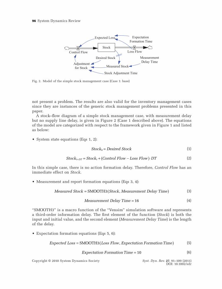
A stock–fl ow diagram of a simple stock management case, with measurement delay but no supply line delay, is given in Figure 2 (Case 1 described above). The equations of the model are categorized with respect to the framework given in Figure 1 and listed as below:

• System state equations (Eqs 1, 2):

Stock Desired Stock0 = (1)

Stock Stock Control Flow Loss Flow DTt DT t+ = + −( )⋅ (2)

In t his simple case, there is no action formation delay. Therefore, Control Flow has an immediate effect on Stock.

• Measurement and report formation equations (Eqs 3, 4):

Measured Stock Stock Measurement Delay Time= ( )SMOOTH3 , (3)

Measurement Delay Time = 16 (4)

“SMO OTH3” is a macro function of the “Vensim” simulation software and represents a third-order information delay. The fi rst element of the function (Stock) is both the input and initial value, and the second element (Measurement Delay Time) is the length of the delay.

• Expectation formation equations (Eqs 5, 6):

Expected Loss Loss Flow Expectation Formation Time= ( )SMOOTH3 , (5)

Expectation Formation Time = 10 (6)

StockLoss FlowControl Flow

Adjustmentfor Stock

Stock Adjustment Time

Desired Stock MeasurementDelay Time

ExpectationFormation Time

Expected Loss

Measured Stock

Fig. 2. Model of the simple stock management case ( Case 1: base)



Expe cted Loss is equal to Loss Flow and remains constant from beginning to end of every simulation run presented in this paper, because Loss Flow itself is assumed to be a constant. Still, we used an information delay function in the expectation formation formulation (Eq. 5) in order to refl ect the fact that it is usually the expected value of Loss Flow used in decision making, not the actual value of it.

• Base decision formation equations (Eqs 7–9):

Control Flow Expected Loss Adjustment for Stock= + (7)

Adjustment for StockDesired Stock Measured Stock

Stock Adjustme= −

nnt Time (8)

Stock Adjustment Time = 5 (9)

The a bove standard decision heuristic is often called the anchor-and-adjust formulation in the literature. Here we assume that there are no delays involved in decision making. Accordingly, the base anchor-and-adjust decision heuristic (Eqs 7–9) refl ects our assump-tion that decisions are made instantaneously.

• External force equations (Eqs 10, 11):

Loss Flow = 1 (10)

Desired Stock = + ( )9 1 4STEP , (11)

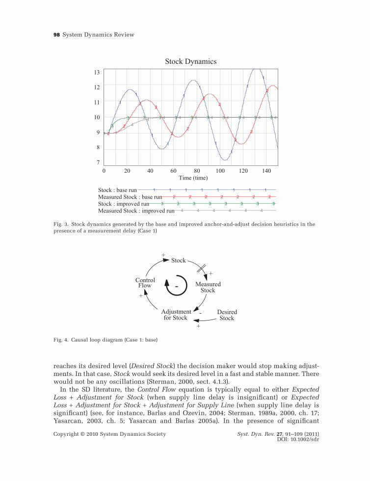
The s ystem state is started on its equilibrium point. Later, at time = 4, a shock is given to the system by changing the Desired Stock value. The resulting Stock behavior that can be seen in Figure 3 (fi rst line) is highly oscillatory.2 According to the base anchor-and-adjust decision heuristic (Eqs 7–9), the decision maker makes adjustments until Measured Stock reaches Desired Stock level. By the time Measured Stock becomes equal to Desired Stock, the actual Stock becomes much higher. Therefore, Measured Stock does not stop at Desired Stock level but keeps on increasing towards its goal, the actual Stock level. When Measured Stock crosses Desired Stock level, the decision maker starts to make negative adjustments that cause a decrease in the Stock level. However, Mea-sured Stock continues increasing, since, although Stock is decreasing, it is still higher than Measured Stock. Measured Stock keeps increasing and even crosses its own goal (Stock), because the measurement delay makes it impossible to recognize sudden changes in Stock. See the dynamics of lines 1 and 2 in Figure 3 approximately within the time ranges of 0–35, 65–90 and 120–145. As Stock goes further down, Measured Stock also starts following it. Again, Measured Stock does not stop at Desired Stock level, since, by the time it reaches the desired level, Stock is at a much lower point. Measured Stock keeps decreasing and even crosses Stock level. See the dynamics of lines 1 and 2 in Figure 3 approximately within the time ranges of 35–65 and 90–120. It is the delay (see Figures 2 and 4; Eqs 3 and 4) in perceiving the actual Stock level, which causes the decision maker to overcorrect. If there was not any delay in the system, once Stock



reaches its desired level (Desired Stock) the decision maker would stop making adjust-ments. In that case, Stock would seek its desired level in a fast and stable manner. There would not be any oscillations (Sterman, 2000, sect. 4.1.3).

In the SD literature, the Control Flow equation is typically equal to either Expected Loss + Adjustment for Stock (when supply line delay is insignifi cant) or Expected Loss + Adjustment for Stock + Adjustment for Supply Line (when supply line delay is signifi cant) (see, for instance, Barlas and Ozevin, 2004; Sterman, 1989a, 2000, ch. 17; Yasarcan, 2003, ch. 5; Yasarcan and Barlas 2005a). In the presence of signifi cant

Stock Dynamics13

12

11

10

9

8

7

4

44 4 4 4 4 4 4 4 4

3

3 3 3 3 3 3 3 3 3 3

2

2

22

22

2

2

2

2

2

1

1

1

1

1

1

1

1

1

1

1

0 20 40 60 80 100 120 140Time (time)

Stock : base run 1 1 1 1 1 1 1 1

Measured Stock : base run 2 2 2 2 2 2 2

Stock : improved run 3 3 3 3 3 3 3 3

Measured Stock : improved run 4 4 4 4 4 4

Fig. 3. Stock dynamics generated by the base and im proved anchor-and-adjust decision heuristics in the presence of a measurement delay (Case 1)

Adjustmentfor Stock

DesiredStock

+

+

MeasuredStock

-

Stock

ControlFlow

+

+

-

Fig. 4. Causal loop diagram (Case 1: base)



measurement delays, the actual stock value is not available to the decision maker. How can it be possible to manage a stock under this circumstances so that it reaches its desired level in a stable yet fast manner? If it were a material supply line delay instead of the measurement delay, the solution would be the inclusion of the supply line adjust-ment term in the Control Flow equation, together with Adjustment for Stock. Similarly, the existence of the measurement delay also necessitates another adjustment term in the Control Flow equation. Therefore, we suggest a decision-making heuristic which has two adjustment terms: Adjustment for Stock and Adjustment for Past Adjustments. The model with the improved anchor-and-adjust decision heuristic, which prevents overcor-rection, is given in Figure 5.

The system state equations (Eqs 1, 2), measurement and report formation equations (Eqs 3, 4), expectation formation equations (Eqs 5, 6), decision formation equations (Eqs 8, 9), and external force equations (Eqs 10, 11) are kept unchanged for the model in Figure 5. The only updated equation is the Control Flow equation (Eq. 7). There are also additional decision formation equations in the improved anchor-and-adjust formulation given below:

• Improved decision formation equations (Eqs 8, 9, 12–19):

Control Flow Expected Loss Total Adjustment= + (12)

Past Adjustments0 0= (13)

Past Adjustments Past Adjustments Total AdjustmentRem

t DT t+ = + (( −ooving Past Adjustments DT)⋅ )

(14)

Total Adjustment Adjustment for Stock Adjustment for Past Adjust= + mments (15)

Weight of PastAdjustments

PastAdjustments

Total Adjustment

Adjustment forPast Adjustments

RemovingDelay Time

Removing PastAdjustments

StockLoss FlowControl Flow

Adjustmentfor Stock

StockAdjustment

Time

DesiredStock

MeasurementDelay Time


Expected Loss

Measured Stock

Fig. 5. Model of the simple stock management case w ith the improved anchor-and-adjust decision heuristic (Case 1: improved)



Adjustment for Past Adjustments Weight of Past Adjustments

Past

= ⋅

− AAdjustmentsStock Adjustment Time

⎛⎝⎜

⎞⎠⎟

(16)

Weight of Past Adjustments = 1 (17)

Removing Past AdjustmentsTotal Adjustment Removing Del

= DELAY I3, aay Time

Past AdjustmentsRemoving Delay Time

,

0

⎛

⎝⎜⎜

⎞

⎠⎟⎟

(18)

Removing Delay Time Measurement Delay Time= (19)

For simplici ty, Removing Past Adjustments (Eq. 18) is formulated as a third order mate-rial delay with using DELAY3I macro function of Vensim. The input of this macro is Total Adjustment. As we need the total stock value accumulated in this third-order delay, we compute it by defi ning an artifi cial stock called Past Adjustments (Eq. 14). In reality, there are three cascaded fi rst-order material delay stocks and the values of these stocks are calculated implicitly by the software. The value of the Past Adjustments stock is equal to the sum of these three implicit stocks. This is possible after setting the initial value of the artifi cial stock equal to the sum of the initial values of three implicit stocks. In Figures 5 and 6, the positive link from Past Adjustments to Removing Past Adjust-ments fl ow represents the link that exists between the last implicit stock of the third order delay macro and its outfl ow.

The fi rst feedback loop in Figure 6, which consists of Stock, Measured Stock, Adjust-ment for Stock, Total Adjustment, and Control Flow, is the same as the feedback loop given in Figure 4 except for an additional variable, Total Adjustment. The aim of this loop is to make Stock seek Desired Stock. However, the delay between Stock and Mea-surement Delay causes overcorrection, which results in unwanted oscillations. The improved anchor-and-adjust decision heuristic (Eqs 8, 9, 12–19) adds two more feedback loops to the model. The aim of the second feedback loop in Figure 6, which is formed by Total Adjustment, Past Adjustments, and Adjustment for Past Adjustments, is to prevent overcorrection by taking Past Adjustments into consideration. The aim of the third feedback loop, which consists of Past Adjustments and Removing Past


Adjustmentfor Stock Desired

Stock+

MeasuredStock

-

StockControlFlow

+

+

TotalAdjustment

+

PastAdjustments

+

-+

+


+

-

-- -

Fig. 6. Causal loop diagram (Case 1: improved)



Adjustments, is to make the Past Adjustments stock decay in time. As the effect of Total Adjustment on Stock is perceived (i.e., refl ected in Measured Stock) after a delay, that much adjustment should simultaneously be removed from Past Adjustments stock. In order to achieve simultaneity, the decay process of Past Adjustments stock should imitate the measurement delay structure.3 For this reason, the order and delay time of the decay process of the Past Adjustments stock is assumed to be the same as the order and delay time of the measurement delay (compare Eqs 18 and 19 with Eqs 3 and 4). In short, the heuristic tries to take into account the past adjustments until their effect reaches Measured Stock.

If we compare the base and improved Stock dynamics (lines 1 and 3 in Figure 3), one can easily see the improvement achieved. The base Stock dynamics (line 1) is highly unstable and oscillatory. In contrast, the improved Stock dynamics (line 3) is perfectly stable and quite fast in approaching the desired level. Thus the improved anchor-and-adjust decision heuristic (Eqs 8, 9, 12–19) is quite successful. Moreover, it is robust; we tested the heuristic with inaccurate parameter values and still obtained reasonable outcomes. The fi rst line in Figure 7 is generated by the model in Figure 2 and is exactly the same as the fi rst line in Figure 3. The second, third, fourth and fi fth lines in Figure 7 are generated by the model in Figure 5. The second line in Figure 7 is exactly the same as the third line in Figure 3. The third line in Figure 7 is obtained by changing the order of the decay process of Past Adjustments stock from 3 to 1. The fourth line in Figure 7 is obtained by setting Removing Delay Time equal to the half of Measurement Delay Time. Finally, the fi fth line in Figure 7 is obtained in the presence of both types of errors (order of the decay process = 1, Removing Delay Time = Measurement Delay

Stock Dynamics

13

12

11

10

9

8

7

55

5 5 5 5 5 54

44

4 4 4 4 4 4

3

33 3 3 3 3 3 3

2

2 2 2 2 2 2 2 2

1

1

1

1

1 1

1

1

1

0 20 40 60 80 100 120 140Time (time)

Stock : base run 1 1 1 1 1 1 1

Stock : improved run 2 2 2 2 2 2 2

Stock : error in order 3 3 3 3 3 3

Stock : error in duration 4 4 4 4 4 4

Stock : error in order and duration 5 5 5 5 5

Fig. 7. Stock dynamics in the presence of inaccurat e parameter values (Case 1)



Time/2). All the four stock dynamics generated by the improved anchor-and-adjust decision heuristic (lines 2–5 in Figure 7) are much better than the stock dynamics generated by the standard anchor-and-adjust decision heuristic (fi rst line in Figure 7). Even under unfavorable conditions, the proposed heuristic is still capable of producing satisfactory stock behavior.

Stock management in the presence of composite delays

The main aim of this section is to demonstrate how the suggested heuristic can be applied when there is more than one type of delay in the system. In order to obtain a composite delay problem, an action formation delay in the form of a fi rst-order material supply line is added to the model in Figure 2 (Case 2 described in the previous section). The resulting model is given in Figure 8.

The system state equation (Eq. 1), measurement and report formation equations (Eqs 3, 4), expectation formation equations (Eqs 5, 6), decision formation equations (Eqs 7–9) and external force equations (Eqs 10, 11), which are valid for the model in Figure 2, are kept unchanged for the model in Figure 8. The only updated equation is the Stock equa-tion (Eq. 2). Moreover, there are new equations representing action formation.

• System state equations (Eqs 1, 20):

Stock Stock Acquisition Flow Loss Flow DTt DT t+ = + −( )⋅ (20)

• Action formation equations (Eqs 21–24):

Supply Line Acquisition Delay Time Expected Loss0 = ⋅ (21)

Supply Line Supply Line Control Flow Acquisition Flow Dt DT t+ = + −( )⋅ TT (22)

Acquisition FlowSupply Line

Acquisition Delay Time= (23)

Acquisition Delay Time = 8 (24)

StockLoss Flow

Adjustmentfor Stock

Stock Adjustment Time

DesiredStock Measurement

Delay Time


Expected Loss

MeasuredStock

Supply LineControl Flow Acquisition Flow

AcquisitionDelay Time

Fig. 8. Model of the stock management case with two types of delay (Case 2: base)



We assume that Su pply Line and Acquisition Flow information are not available to the decision maker. Therefore, we cannot have a Supply Line Adjustment term in the Control Flow equation. The information available to the decision maker can be listed as Expected Loss, Expectation Formation Time, Measured Stock, Measurement Delay Time, Acquisition Delay Time, and orders of measurement and supply line delays. Under these circumstances, the Control Flow equation (Eq. 7) produces highly oscillatory Stock dynamics (fi rst line in Figure 10). Note that the dynamics generated by the model in Figure 8 (fi rst and second lines in Figure 10) is more unstable than the dynamics gener-ated by the model in Figure 2 (fi rst and second lines in Figure 3). This is not surprising, since, if not accounted for, every additional delay increases instability.

The improved anchor-and-adjust decision heuristic given in Figure 5 is modifi ed so as to account also for the supply line delay. The new model with the modifi ed heuristic is given in Figure 9. The system state equations (Eqs 1, 20), measurement and report formation equations (Eqs 3, 4), expectation formation equations (Eqs 5, 6), decision for-mation equations (Eqs 8, 9), external force equations (Eqs 10, 11) and action formation equations (Eqs 21–24), which are valid for the model in Figure 8, are also valid for the model in Figure 9. However, Control Flow equations used in the two models are differ-ent: Eq. 7 is valid for the model in Figure 8 and Eq. 12 is valid for the model in Figure 9. Moreover, in addition to the Control Flow Eq. (12), some of the other improved deci-sion formation equations (Eqs 15–17, 19), which belong to the model in Figure 5, are also valid for the model in Figure 9.

Weight of PastAdjustments

PA1Total Adjustment


TransferringDelay Time

StockLoss Flow

Adjustmentfor Stock

StockAdjustment

Time

DesiredStock

MeasurementDelay Time


Expected Loss

MeasuredStock

SupplyLine Acquisition

FlowControlFlow

AcquisitionDelay Time

PA2Transferring from

PA1 to PA2


RemovingDelay Time

PastAdjustments

Fig. 9. Model of the stock management case with two types of delay and the improved anchor-and-adjust decision heuristic (Case 2: improved)



• Improved decision formation equations (Eqs 8, 9, 12, 15–17, 19, 25–32):

Past Adjustments PA PA= +1 2 (25)

PA1 00 = (26)

PA PA Total Adjustment Transferring from PA to PA DTt DT t1 1 1 2+ = + −( )⋅ (27)

PA2 00 = (28)

PA PA Transferring from PA to PA Removing Past Adjustmet DT t2 2 1 2+ = + − nnts DT( )⋅ (29)

Transferring from PA to PAPA

Transferring Delay Time1 2

1= (30)

Transferring Delay Time Acquisition Delay Time= (31)

Removing Past Adjustments

Transferring from PA to PA Re

=

DELAY I31 2, mmoving Delay Time

PARemoving Delay Time

,

20

⎛

⎝

⎜⎜⎜

⎞

⎠

⎟⎟⎟

(32)

In o rder to obtain an ideal decision formation equation set, the equations should pre-cisely refl ect the delay processes between decisions and their perceived effects. For that reason, there are two stocks in the improved anchor-and-adjust decision heuristic sub-structure: PA1 and PA2. The sum of PA1 and PA2 stocks refl ects the amount of the past adjustments which have yet to have an effect on Measured Stock (the stock value per-ceived by the decision maker). The aim of Transferring from PA1 to PA2 is to imitate the transfer of adjustments from Supply Line to Stock and the aim of Removing Past Adjustments is to imitate the effect of adjustments on the Measured Stock. As the effect of Past Adjustments reaches to Stock, the same amount of adjustment is simultaneously transferred from PA1 to PA2. Similarly, as the effect of Past Adjustments is perceived by the decision maker, the same amount of adjustment is simultaneously removed from PA2.4

The Stock dynamics generated by the base (Eqs 7–9) and improved anchor-and-adjust decision heuristics (Eqs 8, 9, 12, 15–17, 19, 25–32), in the presence of a signifi -cant supply line delay, are compared in Figure 10. The dynamics produced by the improved anchor-and-adjust decision heuristic are much better than the dynamics produced by the base anchor-and-adjust decision heuristic (compare line 3 with line 1 in Figure 10). Thus it can be concluded that the improved anchor-and-adjust decision heuristic is quite successful. Note that introducing a supply line delay results in a delayed response in the stock, which is unavoidable (compare the third lines in Figures 3 and 10).



Practical applications

We now discuss some examples to which the decision-making heuristic suggested in this paper can successfully be applied. The fi rst example is inventory management in the presence of a reporting delay. “In some large organizations, it takes a while to collect and process the data, and pass the resulting information to the inventory manager” (Bensoussan et al., 2008). Bensoussan et al. (2008) report a case: fi nished-goods inven-tory management at an assembly plant. Orders are taken by fax, phone or an online entry system. It takes at least several hours to process and report the sales data to the inventory manager. Therefore, the inventory manager has to base his decisions on the delayed inventory information. The information delay between the actual and reported values of inventory is signifi cant in this case. We presume that the decision-making heuristic suggested in this paper would be useful to dampen oscillations and make it possible to lower the desired level of the fi nished-goods inventory. In this case, fi nished-goods inventory corresponds to Stock, sales corresponds to Loss Flow, on-record fi n-ished-goods inventory level corresponds to Measured Stock and orders for the components corresponds to Control Flow. We assume that assembly start rate and components order rate are synchronized.

Another case is the room temperature regulation by an air-conditioning system. In most cases there is a single temperature sensor assigned to a single room. The tempera-ture of the room is controlled by blowing cold or hot air into the room. Therefore, fi rst the temperature of the air in the room is affected and then the temperature of the objects

Stock Dynamics

13

12

11

10

9

8

7

44

44 4 4 4 4 4 4 4

3

33 3 3 3 3 3 3 3 3

2 2

2

2

2

2

2

2

22

2

1

1

11

1

1

1

11

1

0 20 40 60 80 100 120 140Time (time)

Stock : base run 1 1 1 1 1 1 1 1

Measured Stock : base run 2 2 2 2 2 2 2

Stock : improved run 3 3 3 3 3 3 3 3

Measured Stock : improved run 4 4 4 4 4 4 4

Fig. 10. Stock dynamics generated by the base and i mproved anchor-and-adjust decision heuristics in the presence of supply line and measurement delays (Case 2)



in the room including the temperature sensor itself. The delay in sensing the room temperature results in undesired oscillations of the room temperature around the desired level. In this case, the temperature of the room corresponds to Stock, the tem-perature reported by the sensor corresponds to Measured Stock, and the net rate of change in the room temperature corresponds to Control Flow. Note that to be able to apply the heuristic the rates of increase and decrease in the room temperature are needed under different conditions (while blowing and not blowing air) and settings (cooling, heating, fan speed). The room temperature regulation example can success-fully be applied to most control systems including managerial ones, given that the rates of change for different decisions can at least be roughly estimated.

In some cases, even if immediate access to the stock values is possible, still that may be useless if there is a huge variation in the actual and/or measured values. In such a case, smoothing is necessary to fi lter out the noise. However, smoothing itself intro-duces a delay similar to delays introduced by measurement and reporting (Sterman, 1987a). The heuristic presented in this paper can successfully be utilized in such cases too.

Conclusions

In this paper, we fi rst classifi ed delays based on their structural types, orders, and roles. There are four different categories of roles: measurement delays, decision formation delays, action formation delays, and expectation formation delays. We then introduced a conceptual framework that shows the different roles of delays and their relationships with each other. The SD literature includes many studies on action formation delays. One can also fi nd studies on expectation formation delays. On the contrary, delays caused by “measurement and report formation” are not well studied.

Measurement delays may be long or short and they may have different orders, but they all contribute to the complexity of most feedback control systems. The standard anchor-and-adjust decision heuristics fail to manage a stock in the presence of signifi -cant measurement delays. The main reason is that these heuristics require immediate access to the actual values of the stock and its supply line. However, measurement delays prevent instantaneous access. Therefore, an improvement in these heuristics is needed.

We modeled two cases: a stock management problem only with a measurement delay; and a stock management problem with measurement and supply line delays. In the second model, we further assumed that the value of the supply line is not accessible by the decision maker. The standard control equation that includes Expected Loss and Adjustment for Stock terms failed in both cases by creating unstable oscillations. However, in both cases, our improved control heuristic is capable of bringing the stock to its desired value in a stable and fast way. The proposed heuristic is successful, since it prevents over-adjustment by keeping track of the past adjustments and considering them until their effect is perceived by the decision maker. It is also robust, since it produces reasonable dynamics even with inaccurate parameter values.

Future research on delays and stock management will benefi t from the method intro-duced here. The proposed decision heuristic will be able to deal with many different problem types including different delays, after some minor modifi cations.



Notes

1. To save space and ease reading, we use “measurement delays” in short when refer-ring to “delays caused by measurement and report formation processes”. Furthermore, we assume “perception delays” as a part of “measurement delays”. Sometimes, the measurement delay may purely consist of a perception delay.

2. If it were a material supply line delay in the model instead of the measurement delay (Figure 2), the base anchor-and-adjust decision heuristic (Eqs 7–9) would produce Stock dynamics exactly equal to the dynamics of Measured Stock (line 2 in Figure 3) produced by the measurement delay, given that the order and duration of the supply line delay are the same as the measurement delay.

3. Material and information delays are used to approximate the input–output dynamics of complex delay-causing structures that may overcrowd the model if modeled explicitly (Barlas, 2002; Forrester, 1961; Sterman, 2000). Here, we assume that the measurement delay is an information delay, but the suggested decision-making heu-ristic is formulated as a material delay. The material delay structure in the heuristic will successfully imitate the information delay if Measurement Delay Time is a con-stant. If Measurement Delay Time is not a constant, we need to use its estimated value in the heuristic. In such a case, we suggest using relatively long estimation times. This will prevent transient differences between information and material delay structures from dominating the behavior and allow the heuristic to work as intended.

4. If the decision maker wishes to simplify the decision-making heuristic, she can approximate the ideal decay process by using a single Past Adjustments stock with estimated and aggregated parameter values (i.e., order of the decay process of Past Adjustments = E[order of supply line] + E[order of measurement delay]; Removing Delay Time = E[Acquisition Delay Time] + E[Measurement Delay Time]). This will result in Stock dynamics very similar to the one generated by the ideal decay process.

Acknowledgements

We thank the editor and two anonymous reviewers for their valuable and constructive suggestions.

Biography

Hakan Yasarcan is an Assistant Professor in the Industrial Engineering Department at Bogazici University, Istanbul, Turkey. During this research, he was a research associate at the Accelerated Learning Laboratory, Australian School of Business (Incorporating AGSM), University of New South Wales, Sydney, Australia. He earned all his degrees (BSc, MSc, PhD) in Industrial Engineering, with a PhD from his current institution, Bogazici University (2003). His research interests can be listed as stock management, delays and the other main elements of dynamic complexity, goal formation and adaptive goal setting structures, dynamic decision making, and interactive simulation games. In the past, he taught many industrial engineering core courses at the undergraduate level. Currently, he teaches introductory and advanced courses in system dynamics at the graduate level. He has also been teaching and practicing Sahaja Yoga for the last ten years.



References

Barlas Y. 2002. System dynamics: systemic feedback modeling for policy analysis. In Knowledge for Sustainable development: An Insight into the Encyclopedia of Life Support Systems. UNESCO/EOLSS: Paris and Oxford; 1131–1175.

Barlas Y, Ozevin MG. 2004. Analysis of stock management gaming experiments and alternative ordering formulations. Systems Research and Behavioral Science 21(4): 439–470.

Barlas Y, Yasarcan H. 2006. Goal setting, evaluation, learning and revision: a dynamic modeling approach. Evaluation and Program Planning 29(1): 79–87.

Barlas Y, Yasarcan H. 2008. A comprehensive model of goal dynamics in organizations: setting, evaluation and revision. In Complex Decision Making: Theory and Practice, Qudrat-Ullah H, Spector JM, Davidsen PI (eds). Springer/NECSI: Berlin; 295–320.

Bensoussan A, Cakanyildirim M, Sethi S, Wang M, Zhang H. 2008. Average cost optimality in inventory models with dynamic information delays. Available: http://ssrn.com/abstract=1121440 [24 February 2008].

Diehl E, Sterman JD. 1995. Effects of feedback complexity on dynamic decision making. Organizational Behavior and Human Decision Processes 62(2): 198–215.

Fey WR. 1974. Primary and secondary control of accumulations. In Proceedings for the Fourth Annual Meeting of the Southeast Region of the American Institute for Decision Sciences, 20–23 February, New Orleans, LA.

Forrester JW. 1961. Industrial Dynamics. Pegasus Communications: Waltham, MA.Forrester JW. 1971. Principles of Systems. Pegasus Communications: Waltham, MA.Kawabe T, Nakazawa M, Notsu I, Watanabe Y. 1997. A sliding mode controller for wheel slip ratio

control system. Vehicle System Dynamics 27(5–6): 393–408.Langley PA, Morecroft JDW. 2004. Performance and learning in a simulation of oil industry

dynamics. European Journal of Operational Research 155(3): 715–732.Paich M, Sterman JD. 1993. Boom, bust, and failures to learn in experimental markets. Management

Science 39(12): 1439–1458.Roberts EB. 1978. The design of management control systems, In Managerial Applications

of System Dynamics, Roberts EB (ed.). Pegasus Communications: Waltham, MA; 393–411.

Sterman JD. 1987a. Systems simulation: expectation formation in behavioral simulation models. Behavioral Science 32(3): 190–211.

Sterman JD. 1987b. Testing behavioral simulation models by direct experiment. Management Science 33(12): 1572–1592.

Sterman JD. 1989a. Modeling managerial behavior: misperceptions of feedback in a dynamic decision making experiment. Management Science 35(3): 321–339.

Sterman JD. 1989b. Misperceptions of feedback in dynamic decision making. Organizational Behavior and Human Decision Processes 43(3): 301–335.

Sterman JD. 1994. Learning in and about complex systems. System Dynamics Review 10(2–3): 291–330.

Sterman JD. 2000. Business Dynamics: Systems Thinking and Modeling for a Complex World. Irwin/McGraw-Hill: Boston, MA.

Sterman JD. 2002. All models are wrong: refl ections on becoming a systems scientist. System Dynamics Review 18(4): 501–531.

Yasarcan H. 2003. Feedback, delays and non-linearities in decision structures. PhD Thesis, Bogazici University.

Yasarcan H. 2010. Improving understanding, learning, and performances of novices in dynamic managerial simulation games: a gradual-increase-in-complexity approach. Complexity 15(4): 31–42.



Yasarcan H, Barlas Y. 2005a. A generalized stock control formulation for stock management problems involving composite delays and secondary stocks. System Dynamics Review 21(1): 33–68.

Yasarcan H, Barlas Y. 2005b. Stable stock management heuristics when the outfl ow is propor-tional to the control stock. In Proceedings of The 23rd International System Dynamics Conference, Boston, MA.

NOTES AND INSIGHTS Stock management in the presence of ... · NOTES AND INSIGHTS Stock management...

Documents

Transcript of NOTES AND INSIGHTS Stock management in the presence of ... · NOTES AND INSIGHTS Stock management...