Note Josephson junction 5-16-06 ISS - binghamton.edu ((Brian D. Josephson)) Josephson, Pippard’s...

1

Lecture note on Solid State Physics Josephson junction and DC SQUID

Masatsugu Suzuki and Itsuko S. Suzuki

Department of Physics, State University of New York at Binghamton, Binghamton, New York 13902-6000

(May 17, 2006) Abstract

In the Senior Laboratory (Phys 427) of our Physics Department, an equipment of Mr. SQUID (superconducting quantum interference device) (Star Cryoelectronics, LLC, 25 Bisbee Court, Suite A, Santa Fe, NM 87508) was introduced in the Spring Semester, 2006. It is a DC SQUID magnetometer system incorporating a high-temperature superconductor thin film SQUID sensor chip. This equipment allows one to observe unique features of superconductivity (using liquid nitrogen cooling) such as I-V curve and V-Φ curves. This also allows one to learn about the operation of SQUID by following a series of experiments. This lecture note is intended as a substitute for textbook on Josephson junction, superconductivity, electronics, and related topics. We think that with this lecture note a great deal of background could be provided for undergraduate and graduate students who do not have enough knowledge on the Josephson junction. We use the Mathematica 5.2 for the simulation. All the programs we made are presented here. The Mathematica program is very useful to solving the nonlinear differential equation (numerically) in the Josephson junction and the DC SQUID. Content 1 Introduction 2 Josephson junction

2.1 DC Josephson effect 2.2 AC Josephson effect

3 I-V characteristic of Josephson junction 4 RSJ (Resistively shunted junction) model

4.1 Fundamental equation 4.2 Differential equation for φ 4.3 I-V characteristic for βJ » 1

5 Phase plane analysis 6 Numerical calculation: RSJ model

6.1 Simulation-1 6.2 Simulation-2 6.3 Simulation-3 6.4 Simulation-4 6.5 Simulation-5: the relation of >Ω<>=< Jβη vs κ 6.6 Result on κ vs <η> from simulations

7 DC SQUID (superconducting quantum interference device) 7.1 Current density and flux quantization 7.2 DC SQUID (double junctions): quantum mechanics

2

7.3 Analogy of the diffraction with double slits and single slit 7.4 DC SQUID Junction based on the RSJ model 7.4.1 Formulation 7.4.2 Two-dimensional (2D) SQUID potential 7.5 Simple case: βJ »1 and β = 0 7.6 More general case: βJ »1 and finite β

8 Simulation: DC SQUID 8.1 Relation of <η> vs κB with 0/ ΦΦext as a parameter 8.2 Critical current vs 0/ ΦΦext with β as a parameter 8.3 Relation of <η> vs 0/ ΦΦext with κB as a parameter 8.4 Loop current

9 Conclusion Appendix 1 Introduction

For superconducting tunnel junctions with extremely thin insulating layers (10 – 15 Å) (weak link between the superconductors), the electron pair correlations extend through the insulating barrier. In this situation, it has been predicted by Josephson that paired electrons (Cooper pairs) can tunnel without dissipation from one superconductor to the other superconductor on the opposite side of the insulating layer [B.D. Josephson, Phys. Lett. 1, 251 (1962). The direct supercurrent of pairs, for currents less that Ic, flows with zero-voltage drop across the junction (DC Josephson effect). The width of the insulating barrier of the junction limits the maximum that can flow across the junction, but introduce no resistance in the flow. Josephson also predicted that in the case a constant finite voltage V is established across the junction, an alternating supercurrent Ic sin(ωJt+φ0) flows with frequency ωJ = 2eV/ħ (AC Josephson effect). We solve a nonlinear differential equation for the phase φ using the Mathematica 5.2. The calculations are carried out using ND (solving the differential equations numerically under appropriate initial conditions). The use of Mathematica 5.2 is essential to our understanding the nonlinear behavior of the Josephson junction. 2 Josephson junction1-10

Tunneling if Cooper pairs form a superconductor through a layer of insulator into another superconductor. Such a junction is called a weak link. (i) DC Josephson effect

A DC current flows across the junction in the absence of any electric or magnetic field.

(ii) AC Josephson effect A DC voltage applied across the junction causes rf (radio frequency) current oscillation across the junction.

(iii) Macroscopic long range quantum interference A DC magnetic field applied through a superconducting circuit containing two junctions causes the maximum supercurrent to show interference effects as a function of magnetic field intensity.

3

((Brian D. Josephson)) Josephson, Pippard’s graduate student at Cambridge, attending Philip Anderson’s lectures there in 1961 to 1962, became fascinated by the concept of the phase of the BCS-GL order parameter as a manifestation of the quantum theory on a macroscopic scale. Playing with the theory of Giaver tunneling, Josephson found a phase-dependent term in the current; he then worked out all the consequences in a series of papers, private letters, and a privately circulated fellowship thesis. In particular, Josephson predicted that a direct current should flow, without any applied voltage, between two superconductors separated by a thin insulating layer. This current would come as a consequence of the tunneling of electron pairs between the superconductors, and the current would be proportional to the sine of the phase difference between the superconductors. At a finite applied voltage V, an alternating supercurrent of frequency 2eV/h should flow between the superconductors. Josephson’s work established the phase as a fundamental variable in superconductivity.(Book edited by Hoddeson et al.12). 2.1 DC Josephson effect3

Fig.1 Schematic diagram for experiment of DC Josephson effect. Two superconductors

SI and SII (the same metals) are separated by a very thin insulating layer (denoted by green). A DC Josephson supercurrent (up to a maximum value Ic) flows without dissipation through the insulating layer.

Let 1ψ be the probability amplitude of electron pairs on one side of a junction. Let 2ψ

be the probability amplitude of electron pairs on the other side. For simplicity, let both superconductors be identical.

4

12

21 ,

ψψ

ψψ

Tt

i

Tt

i

hh

hh

=∂

∂

=∂

∂

where Th is the effect of the electron-pair coupling or (transfer interaction across the insulator). T(1/s) is the measure of the leakage of 1ψ into the region 2, and of 2ψ into the region 1. Let

2

1

22

11 ,

θ

θ

ψ

ψ

i

i

en

en

=

=

where

22

2

12

1

n

n

=

=

ψ

ψ

______________________________________________________________________ ((Mathematica5.2)) Program-1 eq1= — D[ψ1[t],t] — T ψ2[t]

— ψ1 @tD T — ψ2@tD eq2= — D[ψ2[t],t] — T ψ1[t]

— ψ2 @tD T — ψ1@tD

rule1 = 9ψ1 → Jè!!!!!!!!!!!!!!n1@#D Exp@ θ1@#DD &N=

9ψ1 → Iè!!!!!!!!!!!!!!!!n1@#1D θ1@#1D &M=

rule2 = 9ψ2 → Jè!!!!!!!!!!!!!!n2@#D Exp@ θ2@#DD &N=

9ψ2 → Iè!!!!!!!!!!!!!!!!n2@#1D θ2@#1D &M= eq3=eq1/.rule1/.rule2//Simplify

θ1@tD — Hn1 @tD + 2 n1@tD θ1 @tDL2 è!!!!!!!!!!!!!!n1@tD

θ2@tD T —è!!!!!!!!!!!!!!n2@tD

eq4=eq2/.rule1/.rule2//Simplify

θ2@tD — Hn2 @tD + 2 n2@tD θ2 @tDL2 è!!!!!!!!!!!!!!n2@tD

θ1@tD T —è!!!!!!!!!!!!!!n1@tD

______________________________________________________________________ Then we have

δθ ienniTt

intn

211

11

21

−=∂

∂+

∂∂ (3)

5

δθ ienniTt

int

n −−=∂

∂+

∂∂

212

22

21 (4)

where 12 θθδ −= .

Now equate the real and imaginary parts of Eqs.(3) and (4),

δθ

δθ

δ

δ

cos

cos

sin2

sin2

2

12

1

21

212

211

nnT

t

nnT

t

nnTt

n

nnTt

n

−=∂

∂

−=∂

∂

−=∂

∂

=∂

∂

If 21 nn ≈ as for identical superconductors 1 and 2, we have

tt ∂∂

=∂

∂ 21 θθ or 0)( 12 =∂−∂t

θθ .

tn

tn

∂∂

−=∂∂ 21

The current flow from the superconductor S1 and to the superconductor S2 is proportional

to t

n∂

∂ 2 . J is the current of superconductor pairs across the junction

)sin( 120 θθ −= JJ , where J0 is proportional to T (transfer interaction).

φsin0II = . (5) 2.2 AC Josephson effect3

Fig.2 Schematic diagram for experiment of AC Josephson effect. A finite DC voltage is

applied across both the ends.

6

Let a dc voltage V be applied across the junction. An electron pair experiences a potential energy difference qV on passing across the junction (q = -2e). We can say that a pair on one side is at –eV and a pair on the other side is at eV.

212

121

ψψψ

ψψψ

eVTt

i

eVTt

i

+=∂

∂

−=∂

∂

hh

hh

,

or δθ ienniTieVn

tin

tn

2111

11

21

−=∂

∂+

∂∂

h, (6)

δθ ienniTieVnt

int

n −−−=∂

∂+

∂∂

2122

22

21

h. (7)

This equation breaks up into the real part and imaginary part,

δθ

δθ

δ

δ

cos

cos

sin2

sin2

2

12

1

21

212

211

nnTeV

t

nnTeV

t

nnTt

n

nnTt

n

−−=∂

∂

−=∂

∂

−=∂

∂

=∂

∂

h

h

.

From these two equations with 21 nn = ,

h

eVtt

2)( 12 −=∂∂

=∂−∂ δθθ .

)](sin[0 tJJ δ= . with

∫−= Vdteth

2)0()( δδ .

When V = V0 = constant, we have

tVet 02)0()(h

−= δδ .

]2)0(sin[ 00 tVeJJh

−= δ . (8)

The current oscillates with frequency

Veh

20 =ω . (9)

A DC voltage of 1 μV produces a frequency of 483.5935 MHz.

Veh

& 2=φ . (10)

7

((Note)) Suppose that V = V0 = 1 μV. The corresponding frequency ν0 is estimated from the relation,

00 22 πν=

h

eV ,

or

MHzeV 5935.4831005459.12

10)1060219.1(222

27

6120

0 =××

×××== −

−−

ππν

h.

3 I-V characteristic of Josephson junction5,7,8

We now consider the I-V characteristic of the Josephson tunneling junction where a insulating layer is sandwiched between two superconducting layers (the same type). A capacitor is formed by these two superconductors. In this type of Josephson junctions, one can see the quasi-particle I-V curve which is different with increasing voltage and decreasing voltage (hysteresis). There are two voltage states, 0 V and 2Δ/e, where Δ is an energy gap of each superconductor. The I-V curve is characterized by (i) maximum Josephson tunneling current of Cooper pairs at V = 0 and (ii) Quasi-particle tunneling current (V>2Δ/e).

Fig.3 Schematic diagram of quasi-particle I-V characteristic (usually observed in a S-I-S

Josephson tunneling-type). Josephson current (up to a maximum value Ic) flows at V = 0. Δ is an energy gap of the superconductor . The DC Josepson supercurrent flows under V = 0. For V>2Δ/e the quasi-particle tunneling current is seen.

The strong nonlinearity in the quasi-particle I-V curve of a tunneling junction is not

an appropriate to the application to the SQUID element. This nonlineraity can be removed by the use of thin normal film deposited across the electrodes. In this effective resistance is a parallel combination of the junction. The I-V characteristic has no hysteresis. Such behavior is often observed in the bridge-type Josephson junction where two superconducting thin films are bridged by a very narrow superconducting thin film.

8

Fig.4 Schematic diagram of I-V characteristic of a Josephson junction (usually observed

in bridge-type junction), which is reversible on increasing and decreasing V. A Josephson supercurrent flows up to Ic at V = 0. A transition occurs from the V = 0 state to a finite voltage state for I>Ic.. Above this voltage the I-V characteristic exhibits an Ohm’s law with a finite resistance of the Junction. The current has a oscillatory component of angular frequency ω (= 2eV/ħ) (the AC Josephson effect).

4. RSJ (Resistively shunted junction) model: Josephson junction circuit

application7 Here we discuss the I-V characteristics of a Josephson tunneling junction using an

equivalent circuit shown below. This circuit includes the effect of various dissipative processes and the distributed capacity with so-called lumped circuit parameters (connection of R and C in parallel). 4.1 Fundamental equation

9

Fig.5 Equivalent circuit of a real Josephson junction with a current noise source. (RSJ model). J.J. stands for the Josephson junction.

We now consider an equivalent circuit for the Josephson junction, which is described above. J.J. stands for the Josephson junction.

ItIVCRVI Nc =+++ )(sin &φ , (11)

where the first term is a Josephson current, the second term is an Ohmic current, the third term is a displacement current, and IN(t) is the noise current source. Since

Veh

& 2=φ ,

we get a second-order differential equation for the phase φ

)()(2)(sin22

tIUetIIIeRe

CNNc −

∂∂

−=−−=+φφφφφ

h&h&&h , (12)

where U(φ) is an equivalent potential and is defined by

)cos()cos(2

)cos(2

)( 00 φκφφφπ

φφπ

φ +−=+Φ

−=+Φ

−= Jc

cc EIII

cII

cU ,

with κ = I/Ic, where Φ0 (=2πħc/2e = 2.06783372x10-7 Gauss cm2) is a magnetic quantum flux and )2/(0 cIE cJ πΦ= is the Josephson coupling constant. If φ is regarded as the coordinate x, the above equation corresponds to the equation of motion of a mass with

Ce 2)2/(h in the presence of the potential U(φ). The second term of the left-hand side is a friction proportional to the velocity. When IN(t) = 0 and the second term is neglected, the above equation can be rewritten as

constEUCe

==+⎟⎠⎞

⎜⎝⎛ )(

221 2

2

φφ&h , (13)

where E is the total energy and is constant. For κ>1 (or I>Ic), U(φ) monotonically decreases with increasing φ: dφ/dt≠0 (finite voltage-state). For κ<1 (or I<Ic), U(φ) has local minima. There are two solutions: dφ/dt = 0 (no voltage state) or dφ/dt≠0 (finite voltage-state) for large C. In this case, the I-V characteristic has a hysteresis. __________________________________________________________________ ((Mathematica 5.2)) Program-2 U1=-( κ φ + Cos[φ]);Plot[Evaluate[Table[U1,κ,0,1,0.05]],φ,0,6 π, PlotStyle→Table[Hue[0.1 i],i,0,10],Prolog→AbsoluteThickness[2],Background→GrayLevel[0.7], AxesLabel→φ,U(φ),PlotRange→0,6 π,-20,1]

10

2.5 5 7.5 10 12.5 15 17.58φ<

-20

-15

-10

-5

8U φ<

( Graphics ) Plot[Evaluate[Table[U1,κ,1,3,0.2]],φ,0,6 π, PlotStyle→Table[Hue[0.1 i],i,0,10],Prolog→AbsoluteThickness[2],Background→GrayLevel[0.7], AxesLabel→φ,U(φ),PlotRange→0,6 π,-60,1]

2.5 5 7.5 10 12.5 15 17.58φ<

-60

-50

-40

-30

-20

-10

8U φ<

( Graphics ) Fig.6 Equivalent potential energy U(φ) with a parameter κ = I/Ic. (a) 0<κ<1. U(φ) has

local maxima and local minima. (b) 1<κ<3. U(φ) increases with increasing φ. Analogy: Simple rigid pendulum

11

Fig.7 Simple pendulum with an applied torque. We consider a simple rigid pendulum light stiff rod of length l with a bob of mass m.

Fig.8 Free body diagram of the simple pendulum

The pendulum can rotate freely about the pivot P. The equation of motion is given by θηθθ &&& −−= sinmglTI ,

where T is an external torque, I is a moment of inertia around the pivot P and the third term of the right-hand side is a viscosity of air. There is an analogy between this pendulum and the Josephson junction,

θθηθ sinmglIT +++= &&& (pendulum). (14)

φφφ sin22 cIeRe

CI ++= &h&&h (Josephson). (15)

12

Table 1 ________________________________________________________________________ Josephson junction pendulum phase difference φ deflection θ total current across junction I applied torque T Capacitance C Moment of inertia normal tunneling conductance 1/R viscous damping η Josephson current Icsinφ horizontal displacement of bob θsinlx = voltage across junction V angular velocity θω &= ________________________________________________________________________

(1) θsinmglT = , 0==dtdθω .

When a small torque is applied, the pendulum finally settles down at a constant angle of deflection θ. No angular velocity (ω = 0) corresponds to no voltage across a junction (V = 0). The junction is superconducting. x = l sinθ.

(2) If the torque is gradually increased, the pendulum deflects to a greater but steady angle. We can pass more current through a junction without any voltage appearing.

(3) Critical torque (Tc = mgl). This is the torque which deflects the pendulum through a right angle so that it is horizontal.

(4) For T>Tc the pendulum cannot remain at rest but rotates continuously. As the pendulum rotates, the horizontal deflection x oscillates. The angular velocity is always in the same direction. This corresponds to the case of I>Ic and V≠0. A DC voltage will appear across the junction if the current passed through it exceeds a critical value.

On the half-cycle during which the bob is rising, the rotation decelerates because gravity opposes the applied torque, but on the following half-cycle the bob is accelerated by gravity as it falls.

dcVedtd

hπθ

πν

22

21

== .

The phase is in one-to one correspondence with an angle of rotation of a damped pendulum, driven by a constant torque, in a constant gravitational field. The regime I<Ic corresponds to a situation in which the applied torque is less than a critical torque necessary to raise the pendulum to an angle π/2. For I>Ic the pendulum rotates in a manner such that the average energy dissipated per rotation is equal to the average work per rotation. ________________________________________________________________________ 4.2 Differential equation for φ

For the sake of simplicity, we use the dimensionless quantities. Here we assume that

13

,RI

Vc

=η cII

=κ , tJωτ = ,

where Jω is the Josephson plasma frequency and is defined by 2/12

⎟⎠⎞

⎜⎝⎛=

CeIc

Jh

ω ,

Jdd

dtd

dd

dtd ω

τφτ

τφφ

== .

Similarly we have

2

22

2

2

τφωφ

dd

dtd

J= .

Then we get

)(sin22 2

22 τκκφ

τφω

τφω NJ

cJ

c dd

eRIdd

eIC

−=++hh ,

or

)(sin2

2

τκκφτφβ

τφ

NJ dd

dd

−=++ , (16)

where

RCCeI

eRIeRIeRI J

c

JcJc

J

c

JJ ωωω

ωωβ 12222

2

====h

hhh .

The normalized voltage is described by

τφβ

τφωφτη

dd

dd

eRIdtd

RIeRIV

Jc

J

cc

====2

12

)( hh ,

since

Veh

& 2=φ .

We are interested in the DC current-voltage characteristic so we need to determine the time averaged voltage

τφβ

τφβφ

ddRI

ddRI

dtd

eV JcJc ===

2h ,

or

τφβη

dd

RIV

Jc

=>=< . (17)

Note that the McCumber parametrer βc is sometimes used in stead of βJ, where βc = 1/βJ2.

4.3 I-V characteristic for βJ » 1

For the special case βJ»1 (small capacitance limit), the above equation is reduced to

κφτφβ =+ sin

dd

J ,

TRId

dd

TRI

ddRIV J

T

JJcβπτ

τφβ

τφβ 0

00 21

=== ∫ ,

14

where T is a period;

JT βκ

π1

22 −

= .

Here

∫∫∫ −===

ππ

φκφβ

τφφτ

2

0

2

00 sind

ddddT J

T

,

or

φφκφκφκ

φφκ

φφκ

φβ

ππππ

ddddT

J

]sin1

sin1[

sinsinsin 000

2

0 ++

−=

++

−=

−= ∫∫∫∫ ,

or

12

2 −=

κπ

β J

T for κ>1,

0=J

Tβ

for κ <1,

So we get

12 2 −== κβπ RIT

RIV cJ

c ,

or

12 −= κRI

V

c

, (18)

or 2

1 ⎟⎟⎠

⎞⎜⎜⎝

⎛+=

RIV

c

κ . (19)

________________________________________________________________________ ((Mathematica 5.2)) Program-3 K1@x_D:= ‡

0

πikjj 1

x− Sin@φD +1

x+ Sin@φDyzz φ; Y1 = K1@xD; Y2= Simplify@Y1, x> 1D

2 π

è!!!!!!!! !! !!!−1 + x2

eq1= V1==

2 π Ic RY2

; eq2 = Solve@eq1, xD

::x → −$%%%%%%%% %% %% %% %% %% %1 +

V12

Ic2 R2>, :x → $%%%%%%%%% %% %% %% %% %%1 +

V12

Ic2 R2>>

I1= $%%%%%%%%%%%%%%%%%%%%1+

V12

Ic2 R2ê.8R → 1, Ic→ 1<

"####### ## ## ##1+ V12

Plot[I1,V1,V1,0,4,PlotStyle→Hue[0],Hue[0.4],Prolog→Ab

15

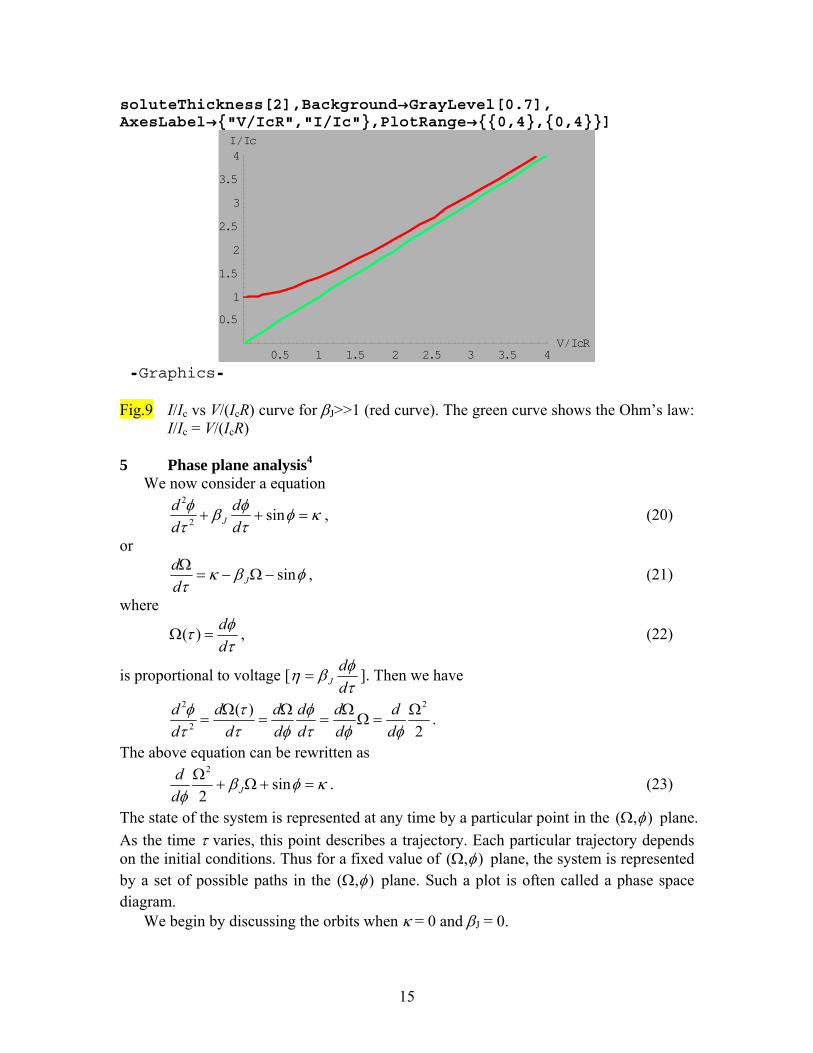
soluteThickness[2],Background→GrayLevel[0.7], AxesLabel→"V/IcR","I/Ic",PlotRange→0,4,0,4]

0.5 1 1.5 2 2.5 3 3.5 4VêIcR

0.5

1

1.5

2

2.5

3

3.5

4IêIc

Graphics

Fig.9 I/Ic vs V/(IcR) curve for βJ>>1 (red curve). The green curve shows the Ohm’s law:

I/Ic = V/(IcR) 5 Phase plane analysis4

We now consider a equation

κφτφβ

τφ

=++ sin2

2

dd

dd

J , (20)

or

φβκτ

sin−Ω−=Ω

Jdd , (21)

where

τφτ

dd

=Ω )( , (22)

is proportional to voltage [τφβη

dd

J= ]. Then we have

2)( 2

2

2 Ω=Ω

Ω=

Ω=

Ω=

φφτφ

φττ

τφ

dd

dd

dd

dd

dd

dd .

The above equation can be rewritten as

κφβφ

=+Ω+Ω sin2

2

Jdd . (23)

The state of the system is represented at any time by a particular point in the ),( φΩ plane. As the time τ varies, this point describes a trajectory. Each particular trajectory depends on the initial conditions. Thus for a fixed value of ),( φΩ plane, the system is represented by a set of possible paths in the ),( φΩ plane. Such a plot is often called a phase space diagram.

We begin by discussing the orbits when κ = 0 and βJ = 0.

16

0sin2

2

=+Ω φ

φdd .

This equation can be integrated as

consta ==−Ω φcos2

2

. (24)

Open orbits require that a always be larger than 2. ______________________________________________________________________ ((Mathematica 5.2)) Program-4 << Graphics ImplicitPlot ; eq1=

12

Ω2 − Cos@φD;

pt1=

ImplicitPlot@eq1 #, 8φ, −2 π, 2 π<, 8Ω, − 2 π, 2 π<, PlotPoints → 100,Contours→ 50, PlotStyle→ [email protected], [email protected]<,DisplayFunction→ Identity, PlotRange→ AllD&ê@ [email protected], 1.2, 0.1D;

Show@pt1, DisplayFunction→ $DisplayFunctionD

-6 -4 -2 2 4 6

-6

-4

-2

2

4

6

Graphics Fig.10 The Ω vs φ plane trajectories. a=−Ω φcos2/2 where a is changed as a

parameter. The closed orbits for a<1 ( 22/)0(2 <=Ω φ ) and the open orbits for a>1 ( 22/)0(2 >=Ω φ ).

6 Numerical calculation

In the plane of the parameters βJ and κ the situation can be summarized as follows.6.7 (a) For κ>1 and arbitrary βJ value no equilibrium point exists; there is only a periodic

solution of the second kind. Therefore the junction will be in the finite voltage state.

(b) For κ<1, the situation is more complicated. The behavior depends on the particular value of βJ.

17

0 0.2 0.4 0.6 0.8 10

0.2

0.4

0.6

0.8

1

κ

β J

Fig.11 Critical line for kc(βJ) (denoted by red line) in the βJ vs κ plane. The blue line

denotes the expression given by JJc βπ

βκ 4)( = . The system undergoes stable

oscillations when κ>κc(βJ) for fixed βJ, in addition to the zero-voltage state.

For βJ<0.2, the simple relation holds: JJc βπ

βκ 4)( = .

A curve can be identified, denoted by κc(βJ), which divides the plane into two regions corresponding to one or two stable state solutions, respectively.

We now solve the differential equation by using Mathematica 5.2

τφτ

dd

=Ω )( ,

and

κτφτβττ

=+Ω+Ω )(sin)()(

Jdd .

Initial condition at τ = 0 (or t = 0): 0)0( v==Ω τ and 0)0( φτφ == .

We calculate the τ dependence of )(τΩ and )(τφ for max0 ττ ≤≤ by using Mathematica 5.2 [NDSolve], where βJ and κ are changed as parameters. (i) Curve of )(τΩ vs )(τφ (ii) The direction of the curves of )(τΩ vs )(τφ , when τ increases [field vector] (iii) The τ dependence of )(τΩ and )(τφ . (iv) The determination of the maximum and minimum values of )(τΩ in the long τ-

region where )(τΩ is a well-defined oscillatory function of τ.

18

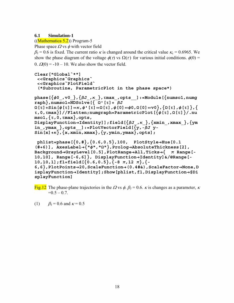
6.1 Simulation-1 ((Mathematica 5.2)) Program-5 Phase space Ω vs φ with vector field βJ = 0.6 is fixed. The current ratio κ is changed around the critical value κc = 0.6965. We show the phase diagram of the voltage φ(τ) vs )(τΩ for various initial conditions. φ(0) = 0. Ω(0) = -10 – 10. We also show the vector field. Clear["Global`*"] <<Graphics`Graphics` <<Graphics`PlotField` (*Subroutine, ParametricPlot in the phase space*) phase[φ0_,v0_,βJ_,κ_,τmax_,opts__]:=Module[numso1,numgraph,numso1=NDSolve[ Ω'[τ]+ βJ Ω[τ]+Sin[φ[τ]] κ,φ'[τ] Ω[τ],φ[0] φ0,Ω[0] v0,Ω[τ],φ[τ],τ,0,τmax]//Flatten;numgraph=ParametricPlot[φ[τ],Ω[τ]/.numso1,τ,0,τmax,opts, DisplayFunction→Identity]];field[βJ_,κ_,xmin_,xmax_,ymin_,ymax_,opts__]:=PlotVectorField[y,-βJ y-Sin[x]+κ,x,xmin,xmax,y,ymin,ymax,opts]; phlist=phase[0,#,0.6,0.5,100, PlotStyle→Hue[0.1 (#+6)], AxesLabel→"φ","Ω",Prolog→AbsoluteThickness[2], Background→GrayLevel[0.5],PlotRange→All,Ticks→ π Range[-10,10], Range[-6,6], DisplayFunction→Identity]&/@Range[-10,10,1];f1=field[0.6,0.5,-8 π,12 π,-6,6,PlotPoints→20,ScaleFunction→(0.4#&),ScaleFactor→None,DisplayFunction→Identity];Show[phlist,f1,DisplayFunction→$DisplayFunction] Fig.12 The phase-plane trajectories in the Ω vs φ. βJ = 0.6. κ is changes as a parameter, κ

=0.5 – 0.7. (1) βJ = 0.6 and κ = 0.5

19

−9 π−8 π−7 π−6 π−5 π−4 π−3 π−2 π−π π2 π3 π4 π5 π6 π7 π8 π9 π10 πφ

-6-5-4-3-2-1

123456

Ω

(2) βJ = 0.6 and κ = 0.6

−2 π−π π 2 π3 π4 π5 π6 π7 π8 π9 π10 πφ

-6-5-4-3-2-1

123456

Ω

(3) βJ = 0.6 and κ = 0.65

−2 π−π π2 π3 π4 π5 π6 π7 π8 π9 π10 πφ

-6-5-4-3-2-1

123456

Ω

20

(4) βJ = 0.6 and κ = 0.67

−2 π−π π2 π3 π4 π5 π6 π7 π8 π9 π10 π11 π12 πφ

-6-5-4-3-2-1

123456

Ω

(5) βJ = 0.6 and κ = 0.69


-6-5-4-3-2-1

123456

Ω

(6) βJ = 0.6 and κ = 0.696


-6-5-4-3-2-1

123456

Ω

21

(7) βJ = 0.6 and κ = 0.6962


-6-5-4-3-2-1

123456

Ω

(8) βJ = 0.6 and κ = 0.6963


-6-5-4-3-2-1

123456

Ω

(9) βJ = 0.6 and κ = 0.6965

A stable periodic solution appears. The states of zero and finite voltage are both possible.

22


-6-5-4-3-2-1

123456

Ω

(10) βJ = 0.6 and κ = 0.697


-6-5-4-3-2-1

123456

Ω

(11) βJ = 0.6 and κ = 0.699


-6-5-4-3-2-1

123456

Ω

23

(12) βJ = 0.6 and κ = 0.7


-6-5-4-3-2-1

123456

Ω

6.2 Simulation-2 ((Mathematica 5.2)) Program-6

βJ = 0.6 is fixed. The current ratio κ is changed around the critical value κc = 0.6965. We show the τ dependence of the voltage )(τΩ for various initial conditions. Note that the normalized DC voltage RIV c/ is defined by Ω>=< Jβη . For κ>κc(βJ), )(τΩ is a

sum of time-independent term )Ω and a periodically oscillating function of τ. The

average voltage corresponds to Ω>=< Jβη , where Ω is the average of the maximum and minimum values of )(τΩ in the long τ- region, where )(τΩ is a well-defined periodically oscillating function of τ. The method to find the maximum and minimum values of )(τΩ will be shown in Sec.5.5 for convenience. phlist=phase[0,#,0.6,0.693,100, PlotStyle→Hue[0.1 (#+6)], AxesLabel→"τ","Ω",Prolog→AbsoluteThickness[2], Background→GrayLevel[0.5],PlotRange→0,30 π,-1,3,Ticks→ π Range[0,50,10], Range[-6,6], DisplayFunction→Identity]&/@Range[-10,10,1];Show[phlist,DisplayFunction→$DisplayFunction] Fig.13 Ω vs τ for βJ = 0.6. The parameter κ is varied as a parameter, κ = 0.693 - .1.20. (1) βJ = 0.6 and κ = 0.693

24

10 π 20 π 30 πτ

-1

1

2

3Ω

(2) βJ = 0.6 and κ = 0.694

10 π 20 π 30 πτ

-1

1

2

3Ω

(3) βJ = 0.6 and κ = 0.695

10 π 20 π 30 πτ

-1

1

2

3Ω

25

(4) βJ = 0.6 and κ = 0.6960

10 π 20 π 30 πτ

-1

1

2

3Ω

(5) βJ = 0.6 and κ = 0.6962

The average voltage η (= )(τβ ΩJ =V/RIc) is equal to 0, where βJ = 0.6 and κ (= I/Ic) = 0.6962, independent of the initial condition Ω(τ = 0).

10 π 20 π 30 πτ

-1

1

2

3Ω

(6) βJ = 0.6 and κ = 0.6965

The average voltage η (= )(τβ ΩJ =V/RIc) is nearly equal to 0.6x0.95 = 0.57 where βJ = 0.6 and κ (= I/Ic) = 0.6965).

26

10 π 20 π 30 πτ

-1

1

2

3Ω

(7) βJ = 0.6 and κ = 0.6970

10 π 20 π 30 πτ

-1

1

2

3Ω

(8) βJ = 0.6 and κ = 0.698

10 π 20 π 30 πτ

-1

1

2

3Ω

27

(9) βJ = 0.6 and κ = 0.70

10 π 20 π 30 πτ

-1

1

2

3Ω

(10) βJ = 0.6 and κ = 0.80

The average voltage η (= )(τβ ΩJ ) is equal to 0.6x1.22656 = 0.7359 and 0.6x0 =0 where βJ = 0.6 and κ (= I/Ic) = 0.8, depending on the initial condition Ω(τ = 0).

10 π 20 π 30 πτ

-1

1

2

3Ω

(11) βJ = 0.6 and κ = 0.90

The average voltage η (= )(τβ ΩJ ) is nearly equal to 0.6x1.429 = 0.8574 and 0.6x0 =0 where βJ = 0.6 and κ (= I/Ic) = 0.9, depending on the initial condition Ω(τ = 0). This implies the existence of the hysteresis behavior. The I-V curve with increasing V is different from that with decreasing V.

28

10 π 20 π 30 πτ

-1

1

2

3Ω

(12) βJ = 0.6 and κ = 1.0

The average voltage η (= )(τβ ΩJ ) is equal to 0.6x1.61579 = 0.9695, where βJ = 0.6 and κ (= I/Ic) = 1.0, independent of the initial condition Ω(τ = 0). This implies no hysteresis behavior.

10 π 20 π 30 πτ

-1

1

2

3Ω

(13) βJ = 0.6 and κ = 1.2

The average voltage η (= )(τβ ΩJ ) is equal to 0.6x1.97065 = 1.1824, where βJ = 0.6 and κ (= I/Ic) = 1.2, independent of the initial condition Ω(τ = 0). This implies no hysteresis behavior.

29

10 π 20 π 30 πτ

-1

1

2

3Ω

6.3 Simulation-3 ((Mathematica 5.2)) Preogram-7

βJ = 0.2 is fixed. The current ratio κ is changed around the critical value κc = 0.253. We show the τ dependence of the voltage )(τΩ for various initial conditions.

Clear["Global`*"] <<Graphics`Graphics` <<Graphics`PlotField` (*Subroutine, ParametricPlot in the phase space*) phase[φ0_,v0_,βJ_,κ_,τmax_,opts__]:=Module[numso1,numgraph,numso1=NDSolve[ Ω'[τ]+ βJ Ω[τ]+Sin[φ[τ]] κ,φ'[τ] Ω[τ],φ[0] φ0,Ω[0] v0,Ω[τ],φ[τ],τ,0,τmax]//Flatten;numgraph=Plot[Ω[τ]/.numso1,τ,0,τmax,opts, DisplayFunction→Identity]] phlist=phase[0,#,0.2,0.24,100, PlotStyle→Hue[0.1 (#+6)], AxesLabel→"τ","Ω",Prolog→AbsoluteThickness[2], Background→GrayLevel[0.5],PlotRange→0,30 π,-1,3,Ticks→ π Range[0,50,10], Range[-6,6], DisplayFunction→Identity]&/@Range[-10,10,1];Show[phlist,DisplayFunction→$DisplayFunction] Fig.14 Ω vs τ for βJ = 0.2. The parameter κ is varied as a parameter, κ = 0.24 - .0.50. (1) βJ = 0.2 and κ = 0.24

30

10 π 20 π 30 πτ

-1

1

2

3Ω

(2) βJ = 0.2 and κ = 0.245

10 π 20 π 30 πτ

-1

1

2

3Ω

(3) βJ = 0.2 and κ = 0.250

10 π 20 π 30 πτ

-1

1

2

3Ω

31

(4) βJ = 0.2 and κ = 0.251

10 π 20 π 30 πτ

-1

1

2

3Ω

(5) βJ = 0.2 and κ = 0.252

10 π 20 π 30 πτ

-1

1

2

3Ω

(6) βJ = 0.2 and κ = 0.253

The average voltage η (= )(τβ ΩJ =V/RIc) is equal to 0.2x1.0269 = 0.20538 and 0.2x0 = 0, where βJ = 0.2 and κ (= I/Ic) = 0.253, depending on the initial condition Ω(τ = 0).

32

10 π 20 π 30 πτ

-1

1

2

3Ω

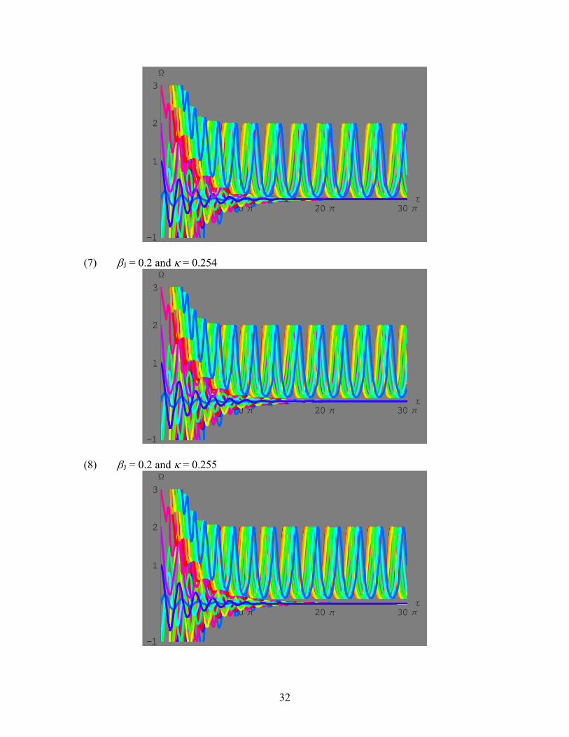
(7) βJ = 0.2 and κ = 0.254

10 π 20 π 30 πτ

-1

1

2

3Ω

(8) βJ = 0.2 and κ = 0.255

10 π 20 π 30 πτ

-1

1

2

3Ω

33

(9) βJ = 0.2 and κ = 0.256

10 π 20 π 30 πτ

-1

1

2

3Ω

(10) βJ = 0.2 and κ = 0.30

10 π 20 π 30 πτ

-1

1

2

3Ω

(11) βJ = 0.2 and κ = 0.4

10 π 20 π 30 πτ

-1

1

2

3Ω

34

(12) βJ = 0.2 and κ = 0.5

The average voltage η (= )(τβ ΩJ =V/RIc) is nearly equal to 0.2x2.48381 = 0.49676 and 0.2x0 = 0, where βJ = 0.2 and κ (= I/Ic) = 0.5, depending on the initial condition Ω(τ = 0). This implies the existence of the hysteresis behavior. The I-V curve with increasing V is different from that with decreasing V.

10 π 20 π 30 πτ

-1

1

2

3Ω

6.4 Simulation-4 ((Mathematica 5.2)) Program-8

βJ = 0.9 is fixed. The current ratio κ is changed around the critical value κc = 0.9197. We show the τ dependence of the voltage )(τΩ for various initial conditions: φ(0) = 0. Ω(0) = -10 – 10. Clear["Global`*"] <<Graphics`Graphics` <<Graphics`PlotField` (*Subroutine, ParametricPlot in the phase space*) phase[φ0_,v0_,βJ_,κ_,τmax_,opts__]:=Module[numso1,numgraph,numso1=NDSolve[ Ω'[τ]+ βJ Ω[τ]+Sin[φ[τ]] κ,φ'[τ] Ω[τ],φ[0] φ0,Ω[0] v0,Ω[τ],φ[τ],τ,0,τmax]//Flatten;numgraph=Plot[Ω[τ]/.numso1,τ,0,τmax,opts, DisplayFunction→Identity]] phlist=phase[0,#,0.9,0.90,100, PlotStyle→Hue[0.1 (#+6)], AxesLabel→"τ","Ω",Prolog→AbsoluteThickness[2], Background→GrayLevel[0.5],PlotRange→0,30 π,-1,3,Ticks→ π Range[0,50,10], Range[-6,6], DisplayFunction→Identity]&/@Range[-10,10,1];Show[phlist,DisplayFunction→$DisplayFunction] Fig.15 Ω vs τ for βJ = 0.9. The parameter κ is varied as a parameter, κ = 0.90 - .2.0.

35

(1) βJ = 0.90 and κ = 0.90

10 π 20 π 30 πτ

-1

1

2

3Ω

(2) βJ = 0.90 and κ = 0.91

10 π 20 π 30 πτ

-1

1

2

3Ω

(3) βJ = 0.90 and κ = 0.915

10 π 20 π 30 πτ

-1

1

2

3Ω

36

(4) βJ = 0.90 and κ = 0.918

10 π 20 π 30 πτ

-1

1

2

3Ω

(5) βJ = 0.90 and κ = 0.919

10 π 20 π 30 πτ

-1

1

2

3Ω

(6) βJ = 0.90 and κ = 0.9195

37

10 π 20 π 30 πτ

-1

1

2

3Ω

(7) βJ = 0.90 and κ = 0.9197

10 π 20 π 30 πτ

-1

1

2

3Ω

(8) βJ = 0.90 and κ = 0.91975

10 π 20 π 30 πτ

-1

1

2

3Ω

38

(9) βJ = 0.90 and κ = 0.9198

10 π 20 π 30 πτ

-1

1

2

3Ω

(10) βJ = 0.90 and κ = 0.92

10 π 20 π 30 πτ

-1

1

2

3Ω

(11) βJ = 0.90 and κ = 0.94

10 π 20 π 30 πτ

-1

1

2

3Ω

39

(12) βJ = 0.90 and κ = 1

The average voltage <η> (= )(τβ ΩJ ) is equal to 0.9x0.98318 = 0.8849 and 0.9x0 =0 where βJ = 0.9 and κ (= I/Ic) = 1.0, depending on the initial condition Ω(τ = 0). This implies the existence of hysteresis behavior.l

10 π 20 π 30 πτ

-1

1

2

3Ω

(13) βJ = 0.90 and κ = 1.1

The average voltage <η> (= )(τβ ΩJ ) is equal to 0.9 x 1.12581 = 1.0132, where βJ = 0.9 and κ (= I/Ic) = 1.1, independent of the initial condition Ω(τ = 0). This implies no hysteresis behavior.

10 π 20 π 30 πτ

-1

1

2

3

4Ω

(14) βJ = 0.90 and κ = 2.0

The average voltage <η> (= )(τβ ΩJ ) is equal to 0.9 x 2.2029 = 1.9826, where βJ = 0.9 and κ (= I/Ic) = 2, which is independent of the initial condition Ω(τ = 0).

40

10 π 20 π 30 πτ

-1

1

2

3Ω

6.5 Simulation-5: the relation of >Ω<>=< Jβη vs κ

Here we show how to determine the average voltage ><η as a function of the current κ, where βJ is changed as a parameter. (1) Using the following Mathematica 5.2 program, we find the maximum and

minimum of Ω(τ) in the long- time region where Ω(τ) periodically oscillates with τ.

(2) The average <Ω> is calculated as (maximum+minimum)/2. The average voltage >Ω<>=< Jβη is plotted as a function of κ for each βJ (= 0.2 – 1.2).

((Mathematica 5.2)) Program-9 Clear["Global`*"] <<Graphics`Graphics` (*Subroutine, to find Maximum and minimum*) phase1[φ0_,v0_,βJ_,κ_,τmax_,opts__]:=Module[numso1,numgraph,numso1=NDSolve[ Ω'[τ]+ βJ Ω[τ]+Sin[φ[τ]] κ,φ'[τ] Ω[τ],φ[0] φ0,Ω[0] v0,Ω[τ],φ[τ],τ,0,τmax]//Flatten;numgraph=Plot[ Ω[τ]/.numso1,τ,0,τmax,opts, DisplayFunction→Identity]];Max1[φ0_,v0_,βJ_,κ_,τmin_,τmax_]:=Module[numso1,numso1=NDSolve[ Ω'[τ]+ βJ Ω[τ]+Sin[φ[τ]] κ,φ'[τ] Ω[τ],φ[0] φ0,Ω[0] v0,Ω[τ],φ[τ],τ,0,τmax]//Flatten;maximum=FindMaximum[βJ Ω[τ]/.numso1,τ,τmin,τmax]];Min1[φ0_,v0_,βJ_,κ_,τmin_,τmax_]:=Module[numso1,numso1=NDSolve[ Ω'[τ]+ βJ Ω[τ]+Sin[φ[τ]] κ,φ'[τ] Ω[τ],φ[0] φ0,Ω[0] v0,Ω[τ],φ[τ],τ,0,τmax]//Flatten;minimum=FindMinimum[ βJ Ω[τ]/.numso1,τ,τmin,τmax]];Sei[βJ_,κ_]:=Module[A1,B1, ave1,list1,A1=Max1[0,#,βJ,κ,20 π,30π]&/@Range[-10,10,1]; B1=Min1[0,#,βJ,κ,20 π,30π]&/@Range[-10,10,1];ave1=(A1+B1)/2;list1=Table[κ,ave1[[k,1]],k,1,21]];Nat1[βJ_]:=Flatten[Table[Sei[βJ,κ],κ,0,3,0.01],1];Saw1

41

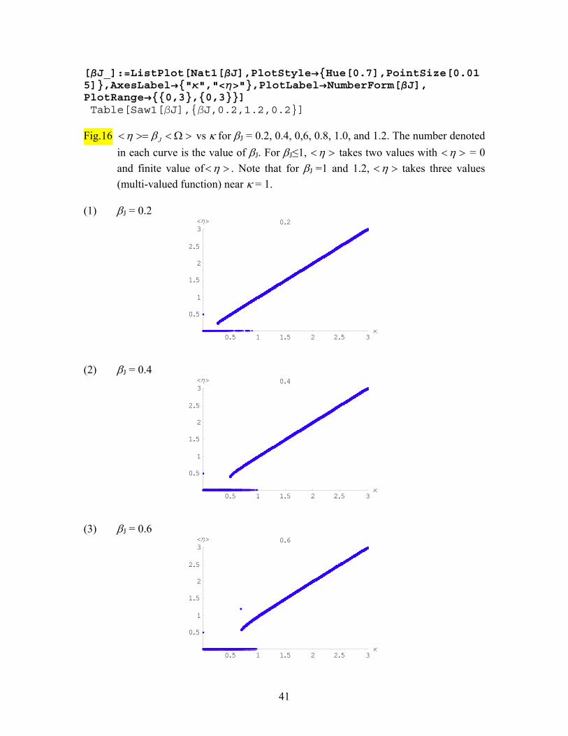
[βJ_]:=ListPlot[Nat1[βJ],PlotStyle→Hue[0.7],PointSize[0.015],AxesLabel→"κ","<η>",PlotLabel→NumberForm[βJ], PlotRange→0,3,0,3] Table[Saw1[βJ],βJ,0.2,1.2,0.2] Fig.16 >Ω<>=< Jβη vs κ for βJ = 0.2, 0.4, 0,6, 0.8, 1.0, and 1.2. The number denoted

in each curve is the value of βJ. For βJ≤1, ><η takes two values with ><η = 0 and finite value of ><η . Note that for βJ =1 and 1.2, ><η takes three values (multi-valued function) near κ = 1.

(1) βJ = 0.2

0.5 1 1.5 2 2.5 3κ

0.5

1

1.5

2

2.5

3<η> 0.2

(2) βJ = 0.4

0.5 1 1.5 2 2.5 3κ

0.5

1

1.5

2

2.5

3<η> 0.4

(3) βJ = 0.6

0.5 1 1.5 2 2.5 3κ

0.5

1

1.5

2

2.5

3<η> 0.6

42

(4) βJ = 0.8

0.5 1 1.5 2 2.5 3κ

0.5

1

1.5

2

2.5

3<η> 0.8

(5) βJ = 1.0

0.5 1 1.5 2 2.5 3κ

0.5

1

1.5

2

2.5

3<η> 1.

(6) βJ = 1.2

0.5 1 1.5 2 2.5 3κ

0.5

1

1.5

2

2.5

3<η> 1.2

6.6 Result on κ vs <η> derived from simulations

Figure 17 shows the <η> vs κ curve for βJ = 0.1 – 1.2. For βJ = 0.6, no voltage drop develops until the value of κ reaches 1. At the point (<η> = 0 and κ = 1) there occurs a transition from the zero-voltage state (<η> = 0) to the finite-voltage state (<η> ≠0). The <η> vs κ curve approaches the straight line denoted by <η> = κ with further increasing <η>. With decreasing <η> from the high <η>-side, in turn, the <η> vs κ curve starts to deviate from the straight line <η> = κ. The transition occurs from the finite-voltage state

43

to the zero-voltage state at κ = 0.6965. Similar hysteresis behaviors are also seen for the cases of βJ = 0.12 - 0.9.

0 0.5 1 1.50

0.5

1

1.5

βJ = 0.1

0.20.3

0.40.50.60.70.80.91.01.2

<η>

κ

Fig.17 The I-V curve (κ vs <η>) for βJ = 0.1 – 1.2.

Fig.18 Schematic diagram of the I-V (κ vs <η>) trajectories as <η. changes. βJ = 0.6. At

<η> = 0, κ changes from 0 to 1. At κ =1, <η> changes from 0 to a value above 1. With further increasing <η>, the relation κ = <η> holds valid (reversible). With decreasing <η>, in turn, the relation κ = <η> still holds valid. There is a transition from this state to the zero-voltage state(<η> = 0) at κ = κc = 0.6965.

7 DC SQUID (superconducting quantum interference device)3

44

7.1 Current density and flux quantization In quantum mechanics, the current density is defined as

AJmc

qmi

q22

** ][2

ψψψψψ −∇−∇=

h ,

where q (=-2e, e>0) is a charge for electron pairs, m is a mass, A is a vector potential, and ψ is a wavefunction. When the wavefunction is given by the amplitude |ψ(r)|and the phase θ(r) as

)()( rr θψψ ie= , then J can be rewritten as

)(2 AJh

h

cq

mq

−∇= θψ .

Note that this current density is invariant under the gauge transformation. χ∇+= AA' and hcq /' χθθ += ,

)()''()''(' 222 AAAJh

h

h

h

h

h

cq

mq

cq

mq

cq

mq

−∇=−∇=−∇= θψθψθψ ,

where ]/)([/ )()()(' hh cqiciq ee χθχ ψψψ +== rrrr . If we consider now a cylinder which may become superconductor in an external magnetic field and if we take a path from a surface at a distance which is larger than the penetration depth λ, then J = 0. When q = -2e, we have

0)2(2 2 =+∇−= AJh

h

ce

me θψ ,

or

Ahce2

−=∇θ ,

0

22222ΦΦ

−=Φ−=⋅−=⋅×∇−=⋅−=⋅∇ ∫∫∫∫ πθhhhh ced

ced

ced

ced aBaAlAl ,

where Φ is the magnetic flux inside the ring and )2/(20 echπ=Φ (=2.06783372 x 10-7 Gauss cm2) is a quantum fluxoid. In the last equation we apply the Stoke’s theorem. ((Note))

The current flows along the ring. However, this current flows only on the surface boundary (region from the surface to the penetration depth λ). Inside of the system (region far from the surface boundary), there is no current since c/4 JH π=×∇ and H = 0 (Meissner effect). 7.2 DC SQUID (double junctions): quantum mechanics

DC SQUID consists of two points contacts in parallel, forming a ring. Each contact forms a Josephson junctions of superconductor 1, insulating layer, and superconductor 2 (S1-I-S2). Suppose that a magnetic flux Φ passes through the interior of the loop.

45

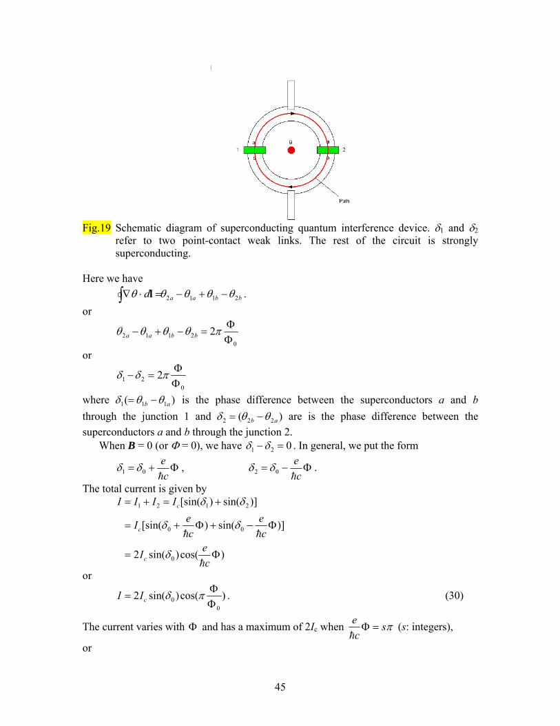
Fig.19 Schematic diagram of superconducting quantum interference device. δ1 and δ2

refer to two point-contact weak links. The rest of the circuit is strongly superconducting.

Here we have

bbaad 2112 θθθθθ −+−=⋅∇∫ l . or

02112 2

ΦΦ

=−+− πθθθθ bbaa

or

021 2

ΦΦ

=− πδδ

where )( 111 ab θθδ −= is the phase difference between the superconductors a and b through the junction 1 and )( 222 ab θθδ −= are is the phase difference between the superconductors a and b through the junction 2.

When B = 0 (or Φ = 0), we have 021 =− δδ . In general, we put the form

Φ+=ceh

01 δδ , Φ−=ceh

02 δδ .

The total current is given by

)cos()sin(2

)]sin()[sin(

)]sin()[sin(

0

00

2121

Φ=

Φ−+Φ+=

+=+=

ceI

ce

ceI

IIII

c

c

c

h

hh

δ

δδ

δδ

or

)cos()sin(20

0 ΦΦ

= πδcII . (30)

The current varies with Φ and has a maximum of 2Ic when πsce

=Φh

(s: integers),

or

46

sse

hcsec

02Φ===Φ

πh . (31)

The simple two point contact device corresponds to a two-slit interference pattern, for which the physically interesting quantity is the modulus of the amplitude rather than the square modulus, as it is for optical interference patterns. 7.3 Analogy of the diffraction with double slits and single slit

Fig.20 Diffraction effect of Josephson junction. A magnetic field B along the z direction,

which is penetrated into the junction (in the normal phase). We consider a junction (1) of rectangular cross section with magnetic field B applied in the plane of the junction, normal to an edge of width w.

]sin[2

110 ∫ ⋅+= lA d

cqJJh

δ ,

with q = -2e. We use the vector potential A given by

)0,2

,2

()(21 BxBy

−=×= rBA ,

)0,0,(' By−=∇+= χAA , where

2Bxy

−=χ .

Then we have

]sin[])(sin[ 1010 yWc

qBJdxByc

qJJb

a

x

x hh−=−+= ∫ δδ ,

dyyWc

qBLJJLdydI ]sin[ 101h

−== δ ,

or

47

∫−

−=2/

2/101 ]sin[

t

t

dyyWc

qBLJIh

δ .

Then we have

)2

sin()sin(2101 Wt

cqB

BWqcLJI

h

h δ= .

Here we introduce the total magnetic flux passing through the area Wt ( BWtW =Φ ), LtJIc 0= , and

ceBWt

ec

BWtW

hh ππ ==ΦΦ

22

0

, or c

eBWtW

h=

ΦΦ

0

π .

Therefore we have

⎟⎟⎠

⎞⎜⎜⎝

⎛ΦΦΦΦ

=

0

011

)sin()sin(

W

W

cIIπ

π

δ .

The total current is given by

⎟⎟⎠

⎞⎜⎜⎝

⎛ΦΦΦΦ

+=+=

0

01111

)sin()]sin()[sin(

W

W

cIIIIπ

π

δδ ,

or

⎟⎟⎠

⎞⎜⎜⎝

⎛ΦΦΦΦ

ΦΦ

=+=

0

0

0011

)sin()cos()sin(2

W

W

cIIIIπ

π

πδ . (32)

The short period variation is produced by interference from the two Josephson junctions, while the long period variation is a diffraction effect and arises from the finite dimensions of each junction. The interference pattern of |I|2 is very similar to the intensity of the Young’s double slits experiment. If the slits have finite width, the intensity must be multiplied by the diffraction pattern of a single slit, and for large angles the oscillations die out. ((Young’s double slit experiment))

We consider the Young’s double slits (the slits are separated by d). Each slit has a finite width a.

48

Fig.21 Geometric construction for describing the Young’s double-slit experiment (not to

scale). ((double slits))

E is the electric field of a light with the wavelength λ. d is the separation distance between the centers of the slits.

Fig.22 A reconstruction of the resultant phasor ER which is the combination of two

phasors (E0).

2cos2 0

αEER = .

The intensity )cos1(22

cos4 20

220

2 αα+==∝ EEEI R .],

where the phase difference α is given by

θλπα sin2 d

= .

((single slit))

We assume that each slit has a finite width a.

49

Fig.23 Phasor diagram for a large number of coherent sources. All the ends of phasors lie

on the circular arc of radius R. The resultant electric field magnitude ER equals the length of the chord.

βRE =0 ,

2

2sin

2sin2

2sin2 0

0

β

ββ

ββ EERER === .

where the phase difference β is given by θλπβ sin2 a

= . Then the resultant intensity I for

the double slits (the distance d) (each slit has a finite width a) is given by

222 )

2

2sin

)(cos1(2

)

2

2sin

(2

cos β

β

αβ

βα

+== mm

III .

_______________________________________________________________________ ((Mathematica 5.2)) Program-10

f@α_, β_D := H1 + Cos@αDLSinA β

2E2

I β

2M2

Plot[Evaluate[Table[f[α,N α],N,20,20],α,-15 π,15 π], PlotPoints→200, PlotStyle→Table[Hue[0.3 i],i,0,10],PlotRange→- 6 π,6 π,0,0.002, Prolog→AbsoluteThickness[1.2],Background→GrayLevel[0.5]]

50

-15 -10 -5 5 10 15

0.00025

0.0005

0.00075

0.001

0.00125

0.0015

0.00175

0.002

Graphics Fig.24 The combined effects of two-slit and single-slit interference. The pattern consists

of a diffraction envelope and interference fringes. 7.4 DC SQUID Juntion based on th RSJ model 7.4.1 Formulation

The DC SQUID consists of two Josephson junctions connected in parallel on a superconducting loop of inductance L.

Fig.25 Simple notation for the DC SQUID consisting of two Josephson junctions (J.J.) in

parallel.

51

Fig.26 Equivalent circuit of the DC SQUID. As shown in Fig.26, the total current is given by

21 IIIB += . The total magnetic flux is given by sext LI+Φ=Φ , where L is the total self-inductance (L = L1 + L2 and L1 = L2 = L/2 in this case)

212 IIIs

−= ,

where Is is the loop (circulating) current.

111

1sin IVCRVIc =++ &φ ,

222

2sin IVCRVIc =++ &φ ,

112 Veh

& =φ , 222 Veh

& =φ .

Since

dtdILVV 1

1 2+= ,

dtdILVV 2

2 2+= , and IB = I1 + I2,

and the total voltage V is given by the simple form,

)(4

)(21

4)(

21 21

2121 dtd

dtd

eVV

dtdILVVV B φφ

+=+=++=h

since 0/ =dtdIB (or IB is independent of t). For the sake of simplicity, we use the dimensionless quantities. Here we assume that

,RI

Vc

=η cII

=κ , tJωτ = .

Then we have

111

21

22 sin

22κφ

τφω

τφω =++

dd

eRIdd

eIC

Jc

Jc

hh ,

or

52

111

21

2

sin κφτφβ

τφ

=++dd

dd

J ,

where

CRcJ ω

β 1= .

Similarly,

222

22

2

sin κφτφβ

τφ

=++dd

dd

J .

We also have Bκκκ =+ 21 ,

sκκκ 212 =− , or

sB κκκ 22 1 −= , where

c

BB I

I=κ ,

cII1

1 =κ , cI

I22 =κ ,

212 κκκ −

==c

ss I

I

Then we have

sB

J dd

dd κκφ

τφβ

τφ

−=++2

sin 11

21

2

. (33)

Similarly we have

sB

J dd

dd κκφ

τφβ

τφ

+=++2

sin 22

22

2

. (34)

The phases are related to the external magnetic flux by

)2

(2)(220000

21 ΦΦ

+=ΦΦ

+Φ

=ΦΦ

=− exts

extsLI κβπππφφ ,

or

)2

(20

21

ΦΦ

−−

= exts π

φφβ

κ , (35)

where

0

2Φ

=LIcβ .

The normalized voltage η is given by

)(21 21

τφ

τφβη

dd

dd

J += . (36)

7.4.2 Two-dimensional (2D) SQUID potential

Equations (33) and (34) describing the DC SQUID dynamics can be regarded as an equation of motion of a point mass in a field of force with a 2D SQUID potential

),( 21 φφU .

1

211

12

12 ),(2

2sin

φφφκκφ

τφβ

τφ

∂∂

−=−+−=+U

Ie

dd

dd

cs

BJ

h

53

and

2

212

22

22 ),(2

2sin

φφφκκφ

τφβ

τφ

∂∂

−=++−=+U

Ie

dd

dd

cs

BJ

h

or

)]2

(22

[sin2

)2

(sin2

),(

0

211

01

1

21

ΦΦ

−−

+−Φ

=+−=∂

∂ extBcs

Bc Ice

IUπ

φφπβ

κφ

πκ

κφ

φφφ h

,

(37)

)]2

(22

[sin2

)2

(sin2

),(

0

212

02

2

21

ΦΦ

−−

−−Φ

=−−=∂

∂ extBcs

Bc Ice

IU πφφπβ

κφπ

κκφφ

φφ h .

(38) Thus the normalized 2D SQUID potential ),(~

21 φφU [= )2/(),( 21 JEU φφ ] is obtained as

)2

(2

)2

cos()2

cos()2

(1),(~ 2121212

0

2121

φφκφφφφπφφπβ

φφ +−

+−−

ΦΦ

−−

= BextU , (39)

where )2/(0 cIE cJ πΦ= is the Josephson coupling constant. It is convenient to introduce new variables

πφφ

221 +

=x , πφφ

221 −

=y .

The loop current κs is related to y as

)(20Φ

Φ−= ext

s yβ

κ .

Then the 2D SQUID potential ),(~21 φφU is rewritten as

)cos()cos(2

)(),(~ 2

0

yxxyyxU Bext πππκβπ

−−ΦΦ

−= .

Here we make a contour plot of ),( 21 φφU in the φ1-φ2 plane. The parameters β (= 1) and Φext/Φ0 (= 0.25) are fixed. The current κB is changed as a parameter. As will be shown in Fig.32, the critical current (κB)c is equal to 1.628 for β = 1 and Φext/Φ0 = 0.25. In Fig.27 we show the contour plot of ),( 21 φφU in the φ1-φ2 plane, where β = 1 and Φext/Φ0 = 0.25. For κB = 0.4, ),( 21 φφU has multiple metasatable state separated by saddle points on the φ2 = φ1 line. With increasing κB, these saddle points gradually disappear. At κ>(κB)c it seems that all the saddle points disappear, suggesting no stable state corresponding to local minima of the potential energy. ((Mathematica 5.2)) Program 11 (*2D SQUID potential,β = 1 - 2,κB = 1 - 3;n0 =Ξ/Φ0 ( 0 - 0.5), pp= points*)

F@φ1_, φ1_, β_, κB_, n0_D :=

π

βJ φ1− φ2

2 π− n0N

2−

κB2

π J φ1+ φ22 π

N− CosAπ J φ1+φ22 π

NECosAπ J φ1− φ22 π

NE

mp[pp_,β_,κB_,n0_]:=Module[ss1,ss2,ss1=ContourPlot[F[φ1,φ1,β,κB,n0], φ1,-4 π, 4 π,φ2,-4 π, 4 π,PlotPoints -> pp, ContourLines ->True,PlotRange -> All, ColorFunction -> Hue,

54

AspectRatio -> Automatic, Compiled→False];ss2=ListContourPlot[ss1[[1]], Contours→(#[[pp/2]]&/@Partition[Sort[Flatten[ss1[[1]]]],pp]), ColorFunction→(Hue[2 #]&),ContourLines→False, MeshRange→-4 π,4 π,-4 π,4 π, DisplayFunction→Identity];Show[ss2, DisplayFunction→$DisplayFunction,FrameTicks→True, AspectRatio→Automatic]] Table[mp[100,1.0,κB,0.25],κB,0,2.0,0.2] Fig. 27 The contour plot of ),( 21 φφU in the in the φ1-φ2 plane: φ1 is x-axis and φ2 is the y

axis. κB = 0.4, 0.8, 1.2, 1.6, and 1.8. β = 1. Φext/Φ0 = 0.25. (κB)c = 1.628. (1) κB =0.4, β = 1.0 and Φ/Φ0 = 0.25

-10 -5 0 5 10

-10

-5

0

5

10

-10 -5 0 5 10

-10

-5

0

5

10

(2) κB =0.8, β = 1.0 and Φ/Φ0 = 0.25

55

-10 -5 0 5 10

-10

-5

0

5

10

-10 -5 0 5 10

-10

-5

0

5

10

(3) κB =1.2, β = 1.0 and Φ/Φ0 = 0.25

-10 -5 0 5 10

-10

-5

0

5

10

-10 -5 0 5 10

-10

-5

0

5

10

(4) κB =1.6, β = 1.0 and Φ/Φ0 = 0.25

56

-10 -5 0 5 10

-10

-5

0

5

10

-10 -5 0 5 10

-10

-5

0

5

10

(5) κB =1.8, β = 1.0 and Φ/Φ0 = 0.25

-10 -5 0 5 10

-10

-5

0

5

10

-10 -5 0 5 10

-10

-5

0

5

10

7.5 Simple case: βJ »1 and β = 0

For simplicity, we assume that βJ »1. This assumption is appropriate for the operation of DC SQUID.

First we consider the critical current at V = 0. We also assume that β = 0.

)]2sin([sin)sin(sin0

112121 ΦΦ

−+=+=+= extccB IIIII πφφφφ ,

57

since

012 2

ΦΦ

−= extπφφ .

Then we have

)cos()sin(200

1 ΦΦ

ΦΦ

−= extextcB II ππφ .

The maximum of IB is

)cos(20

max ΦΦ

= extcII π . (40)

The critical current is a periodic function of the external magnetic flux.

0.5 1 1.5 2 2.5 3ΦextêΦ0

0.5

1

1.5

2

IBêIc

Fig.28 Ideal case for the IB/Ic vs Φext/Φ0 curve in the DC SQUID, where IB is the

maximum supercurrent. IB = 2 Ic when Φ ext/Φ0 = n (integer) and IB = 0 for Φext/Φ0 = n +1/2.

We consider the general case (but still L = 0 and βJ »1)

sB

J dd κκφ

τφβ −=+

2sin 1

1 , (41)

sB

J dd κκφ

τφβ +=+

2sin 2

2 , (42)

012 2

ΦΦ

−= extπφφ . (43)

From the addition of Eqs.(41) and (42) with the help of the relation Eq.(43), we have

2)sin()cos()(

01

001

BextextextJ d

d κπφππφτ

β =ΦΦ

−ΦΦ

+ΦΦ

− .

When we introduce a new parameter

=1ϕ0

1 ΦΦ

− extπφ ,

we have the final form

58

2sin)cos( 1

0

1 BextJ d

d κϕπτϕβ =

ΦΦ

+ . (44)

We are interested in the DC current-voltage characteristic so we need to determine the time averaged voltage

τπβτ

τφβ

τφβφ 2

2 0

111Jc

TJc

Jc RIddd

TRI

ddRI

dtd

eV ==== ∫

h .

Here

')cos(

1sin')cos(sin)cos(

2 0

2

0 1

1

0

2

01

0

12

0 1

1 τπϕκ

φ

π

β

ϕπκφβ

τφφτ

πππ

ΦΦ

=−

ΦΦ

=

ΦΦ

−== ∫∫∫

extext

J

extB

J dd

ddd ,

)cos(2'

0ΦΦ

=ext

B

π

κκ ,

where

φφκφκφκ

φφκ

φφκ

φτππππ

dddd ]sin'1

sin'1[

sin'sin'sin''

000

2

0 ++

−=

++

−=

−= ∫∫∫∫ ,

or

1'2'

2 −=

κπτ for κ>1,

0'=τ for κ <1. Then we have

)cos(1')cos('

2120

2

0 ΦΦ

−=ΦΦ

== extc

extcJc RIRIRIV πκπ

τπ

τβπ ,

or

1')cos( 2

0

−ΦΦ

= κπ ext

cRIV ,

or

c

B

extextc

II

RI

V

)cos(2

1

)cos(1'

0

2

0 ΦΦ

=

⎟⎟⎟⎟

⎠

⎞

⎜⎜⎜⎜

⎝

⎛

ΦΦ

+=ππ

κ ,

or 2

0

2 )()(cos2 c

ext

c

B

RIV

II

+ΦΦ

= π ,

or

)(cos)2

(0

22

ΦΦ

−=>< ext

c

B

c II

RIV π ,

or

59

)(cos42 0

222

ΦΦ

−>=< extcB IIRV π . (45)

When this equation for the voltage is compared with that for one Josephson junction with βJ»1

22cIIRV −= .

We find that the critical current is )/cos(2 0ΦΦextcI π . This means that the critical current is 2Ic for next =ΦΦ 0/ (integer) and zero for next =ΦΦ 0/ +1/2. In other words, the critical current is a periodic function of Φ with a period of 0Φ . However, the actual critical current does not oscillate between 0 and 2Ic because of the finite self-inductance L. In the above model, L (or β = 0) is assumed to be zero. The critical current varies between 2Ic and finite value depending on the value of β (see the detail in Sec.8).

When the total current IB is constant, the voltage across the DC SQUID periodically changes with the external magnetic flux. This is the phenomenon one exploit to create the most sensitive magnetic field detection. ((Note)) Figure 29 is obtained from the Instruction manual of Mr. SQUID.9

Fig.29 Detected voltage vs the magnetic flux Φ/Φ0. The current IB is kept at fixed value

which is a little larger than 2Ic. The detected voltage shows a maximum for Φ = (n+1/2)Φ0, and a minimum for Φ = nΦ0. The detected voltage is a periodic function of Φ with a period of Φ0. (This figure is copied from the User Guide of Mr SQUID9).

7.6 More general case: βJ »1 and finite β

In order to avoid hysteresis in the I-V curve one usually choose over-damped junction. Here we start with the differential equations given by

sB

J dd κκφ

τφβ −=+

2sin 1

1 , (46)

60

sB

J dd κκφ

τφβ +=+

2sin 2

2 , (47)

)2

(20

21 ΦΦ

+=− extsκβπφφ . (48)

or

)2

(2

0

21

ΦΦ

−−

= exts π

φφβ

κ .

Thus we have two differential equations

)2

(22

sin0

211

1

ΦΦ

−−

−=+ extBJ d

dπφφ

βκφ

τφβ ,

)2

(22

sin0

212

2

ΦΦ

−−

+=+ extBJ d

dπφφ

βκφ

τφβ ,

)sinsin(21)(

21

2121 φφκ

τφ

τφβη −−=+= BJ d

ddd ,

where the initial conditions [φ1(0) and φ2(0)] are chosen appropriately 8 Simulation

The differential equations for φ1(τ) and φ2(τ) are numerically solved by using the Mathematica 5.2. We show our calculation on the τ dependence of η. The parameters κB, βJ, β and 0/ ΦΦext are appropriately changed for our calculations. 8.1 Relation of <η> vs κB with 0/ ΦΦext as a parameter

We calculate the relation <η> vs κB where 0/ ΦΦext = 0, 0.05, 0.1, 0.15, 0.20, 0.25, 0.30, 0.35, 0.40, 0.45, and 0.5. We choose βJ = 10 for the over-damped case. So that no hysteresis is seen in the I-V curve. The parameter β is changed as a parameter: β = 0.02 - 3. The voltage <η> suddenly increases from zero to a finite value at the critical current which is dependent on the magnetic flux 0/ ΦΦext and β. (i) Using the following Mathematica 5.2 program, we find the maximum and

minimum of Ω(τ) in the long time region where Ω(τ) periodically oscillates with τ. (ii) The average <Ω> is calculated as (maximum+minimum)/2. The average voltage

>Ω<>=< Jβη is plotted as a function of κ for the fixed βJ (= 10) and β, where the magnetic flux 0/ ΦΦext is changed as a parameter.

(iii) The voltage is equal to zero for κ<(κB)c. It suddenly increase with increasing κ above (κB)c. We determine the critical current (κB)c as a function of the magnetic flux where β is changed as a parameter.

((Mathematica 5.2)) Program-12 Clear["Global`*"] <<Graphics`Graphics` (*Subroutine, DC SQUID beta=1 betaJ=10 voltage vs magnetic flux*)

61

DCSQ@8φ01_, φ02_<, 8βJ_, κB_, β_, N0_<, τmax_, opts__D:=

ModuleA8numso1, numgraph<,

numso1=

NDSolveA9 βJφ1'@τD + Sin@φ1@τDD κB2

−2βJ φ1@τD − φ2@τD

2 π− N0N,

βJφ2'@τD + Sin@φ2@τDD κB2

+2βJ φ1@τD − φ2@τD

2 π− N0N, φ1@0D φ01,

φ2@0D φ02=, 8φ1@τD, φ2@τD<, 8τ, 0, τmax<E êê Flatten;

numgraph= PlotAJ κB− Sin@φ1@τDD −Sin@φ2@τDD2

N ê.numso1, 8τ, 0, τmax<,

opts, DisplayFunction→ IdentityEE;

Max1@8φ01_, φ02_<, 8βJ_, κB_, β_, N0_<, 8τmin_, τmax__<D:=

ModuleA8numso1<,

numso1=



2 π− N0N,



2 π− N0N, φ1@0D φ01,


maximum = FindMaximumAJ κB− Sin@φ1@τDD −Sin@φ2@τDD2

N ê.numso1,

8τ, τmin, τmax<EE;

Min1@8φ01_, φ02_<, 8βJ_, κB_, β_, N0_<, 8τmin_, τmax__<D:=

ModuleA8numso1<,

numso1=



2 π− N0N,



2 π− N0N, φ1@0D φ01,


maximum = FindMinimumAJ κB− Sin@φ1@τDD −Sin@φ2@τDD2

N ê.numso1, 8τ, τmin, τmax<EE

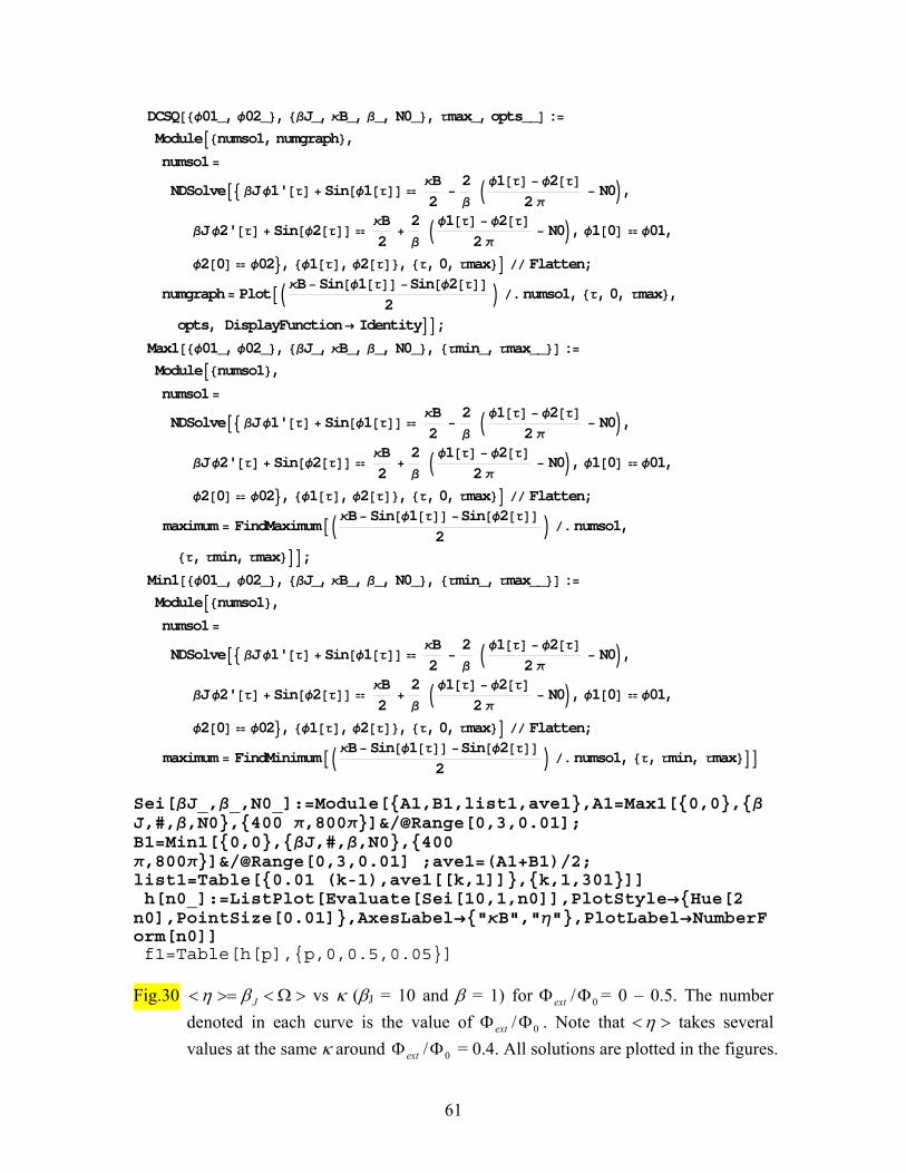
Sei[βJ_,β_,N0_]:=Module[A1,B1,list1,ave1,A1=Max1[0,0,βJ,#,β,N0,400 π,800π]&/@Range[0,3,0.01]; B1=Min1[0,0,βJ,#,β,N0,400 π,800π]&/@Range[0,3,0.01] ;ave1=(A1+B1)/2; list1=Table[0.01 (k-1),ave1[[k,1]],k,1,301]] h[n0_]:=ListPlot[Evaluate[Sei[10,1,n0]],PlotStyle→Hue[2 n0],PointSize[0.01],AxesLabel→"κB","η",PlotLabel→NumberForm[n0]] f1=Table[h[p],p,0,0.5,0.05] Fig.30 >Ω<>=< Jβη vs κ (βJ = 10 and β = 1) for 0/ ΦΦext = 0 – 0.5. The number

denoted in each curve is the value of 0/ ΦΦext . Note that ><η takes several values at the same κ around 0/ ΦΦext = 0.4. All solutions are plotted in the figures.

62

Some values are unphysical. We do not understand why so many values appear. Some solutions may correspond to metastable states.

(1) 0/ ΦΦext = 0. β = 1 and βJ = 10

0.5 1 1.5 2 2.5 3κB

0.25

0.5

0.75

1

1.25

1.5

<η> 0

(2) 0/ ΦΦext = 0.1. β = 1 and βJ = 10

0.5 1 1.5 2 2.5 3κB

0.2

0.4

0.6

0.8

1

1.2

1.4

<η> 0.1

(3) 0/ ΦΦext = 0.2. β = 1 and βJ = 10

0.5 1 1.5 2 2.5 3κB

0.2

0.4

0.6

0.8

1

1.2

<η> 0.2

(4) 0/ ΦΦext = 0.3. β = 1 and βJ = 10

63

0.5 1 1.5 2 2.5 3κB

0.2

0.4

0.6

0.8

1

1.2

<η> 0.3

(5) 0/ ΦΦext = 0.4. β = 1 and βJ = 10

0.5 1 1.5 2 2.5 3κB

0.2

0.4

0.6

0.8

1

1.2

<η> 0.4

(6) 0/ ΦΦext = 0.45. β = 1 and βJ = 10

0.5 1 1.5 2 2.5 3κB

0.2

0.4

0.6

0.8

1

1.2

<η> 0.45

(7) 0/ ΦΦext = 0.5. β = 1 and βJ = 10

64

0.5 1 1.5 2 2.5 3κB

0.2

0.4

0.6

0.8

1

1.2

<η> 0.5

________________________________________________________________________ Fig.31 >Ω<>=< Jβη vs κ (βJ = 10) and (β = 0.3) for 0/ ΦΦext =0 – 0.5. The number

denoted in each curve is the value of 0/ ΦΦext . Note that ><η takes several values at the same κ around 0/ ΦΦext = 0.4 (multi-valued function). All solutions are plotted in the figures. Some values are unphysical. We do not understand why so many values appear. Some solutions correspond to metastable states.

(1) 0/ ΦΦext = 0. β = 0.3 and βJ = 10

0.5 1 1.5 2 2.5 3κB

0.25

0.5

0.75

1

1.25

1.5

<η> 0

(2) 0/ ΦΦext = 0.1. β = 0.3 and βJ = 10

0.5 1 1.5 2 2.5 3κB

0.25

0.5

0.75

1

1.25

1.5

<η> 0.1

65

(3) 0/ ΦΦext = 0.2. β = 0.3 and βJ = 10

0.5 1 1.5 2 2.5 3κB

0.2

0.4

0.6

0.8

1

1.2

1.4

<η> 0.2

(4) 0/ ΦΦext = 0.3. β = 0.3 and βJ = 10

0.5 1 1.5 2 2.5 3κB

0.2

0.4

0.6

0.8

1

1.2

1.4

<η> 0.3

(4) 0/ ΦΦext = 0.4. β = 0.3 and βJ = 10

0.5 1 1.5 2 2.5 3κB

0.2

0.4

0.6

0.8

1

1.2

1.4

<η> 0.4

(5) 0/ ΦΦext = 0.45. β = 0.3 and βJ = 10

66

0.5 1 1.5 2 2.5 3κB

0.2

0.4

0.6

0.8

1

1.2

1.4

<η> 0.45

(6) 0/ ΦΦext = 0.5. β = 0.3 and βJ = 10

0.5 1 1.5 2 2.5 3κB

0.2

0.4

0.6

0.8

1

1.2

1.4

<η> 0.5

8.2 Critical current vs 0/ ΦΦext with β as a parameter

From the above simulation we find that the critical current (κB)c decreases with increasing the magnetic flux from 2 at 0/ ΦΦext = 0 to some finite value (but not zero) at

0/ ΦΦext = 0.5 because of the finite value of β (finite inductance). First we estimate the critical current analytically based on an approximation πφφ /2sin ≈ for |φ|<π/2 (one can easily prove this using the Mathematica 5.2). We use the following approximations,

1112sin φπ

φκ == , 2222sin φπ

φκ == , 2

12 κκκ −=s , 21 κκκ +=B ,

sext

s πκκκπκβπφφ −=−=ΦΦ

+=− )(2

)2

(2 210

21 or sext

s κβκ −=ΦΦ

+0

2 .

From this relation we have

212 12

0

κκβ

κ −=

+ΦΦ

−= exts ,

Bκκκ =+ 21 , )1(

4

021 +Φ

Φ=−

βκκκ Bext ,

or

01 1

22 Φ

Φ+

+= extB

βκκ , (49)

67

02 1

22 Φ

Φ+

−= extB

βκκ .

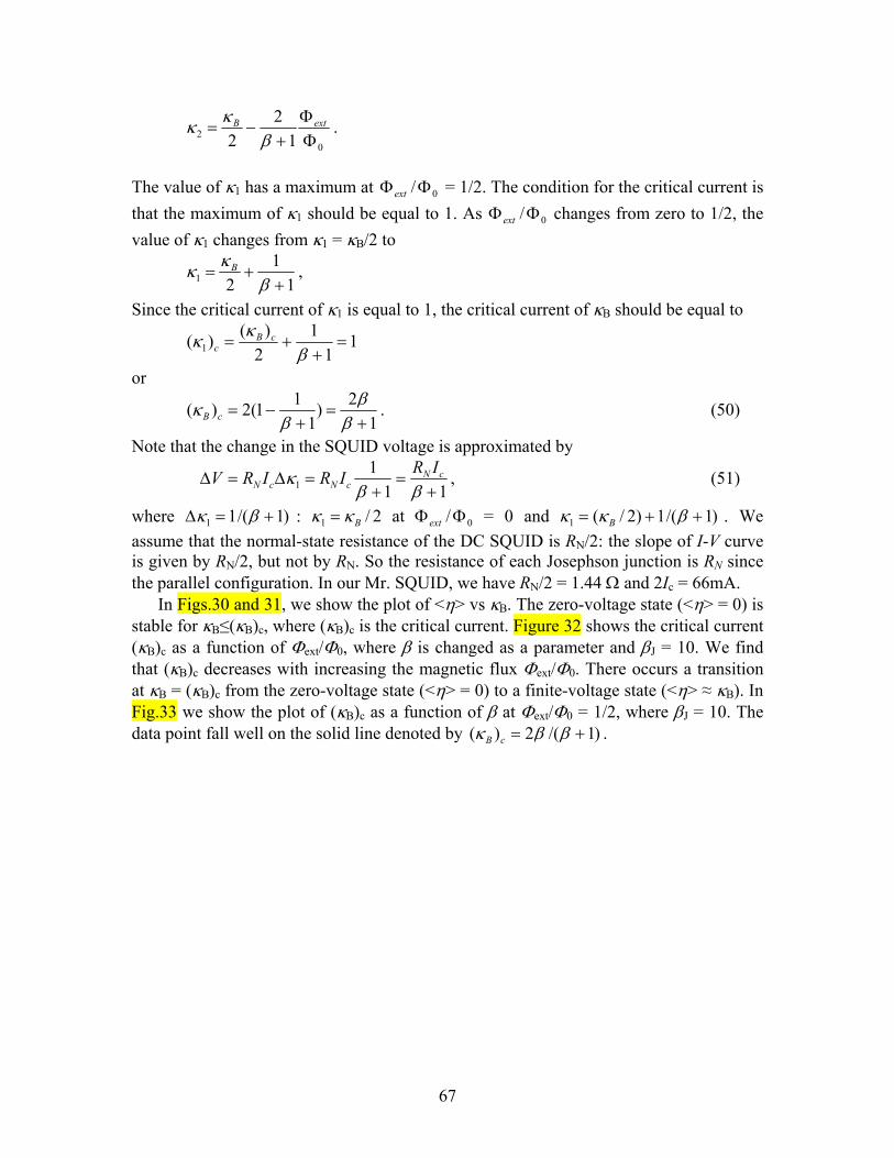
The value of κ1 has a maximum at 0/ ΦΦext = 1/2. The condition for the critical current is that the maximum of κ1 should be equal to 1. As 0/ ΦΦext changes from zero to 1/2, the value of κ1 changes from κ1 = κB/2 to

11

21 ++=

βκκ B ,

Since the critical current of κ1 is equal to 1, the critical current of κB should be equal to

11

12

)()( 1 =+

+=β

κκ cBc

or

12)

111(2)(

+=

+−=

ββ

βκ cB . (50)

Note that the change in the SQUID voltage is approximated by

111

1 +=

+=Δ=Δ

ββκ cN

cNcNIRIRIRV , (51)

where )1/(11 +=Δ βκ : 2/1 Bκκ = at 0/ ΦΦext = 0 and )1/(1)2/(1 ++= βκκ B . We assume that the normal-state resistance of the DC SQUID is RN/2: the slope of I-V curve is given by RN/2, but not by RN. So the resistance of each Josephson junction is RN since the parallel configuration. In our Mr. SQUID, we have RN/2 = 1.44 Ω and 2Ic = 66mA.

In Figs.30 and 31, we show the plot of <η> vs κB. The zero-voltage state (<η> = 0) is stable for κB≤(κB)c, where (κB)c is the critical current. Figure 32 shows the critical current (κB)c as a function of Φext/Φ0, where β is changed as a parameter and βJ = 10. We find that (κB)c decreases with increasing the magnetic flux Φext/Φ0. There occurs a transition at κB = (κB)c from the zero-voltage state (<η> = 0) to a finite-voltage state (<η> ≈ κB). In Fig.33 we show the plot of (κB)c as a function of β at Φext/Φ0 = 1/2, where βJ = 10. The data point fall well on the solid line denoted by )1/(2)( += ββκ cB .

68

0

0.5

1

1.5

2

0 0.1 0.2 0.3 0.4 0.5

β = 0.02 0.30.5 0.8 12

(κB) c

Φ/Φ0

Fig.32 The critical current (κB)c as a function of Φext/Φ0, where β is changed as a

parameter. βJ = 10.

0

0.2

0.4

0.6

0.8

1

1.2

1.4

0 0.5 1 1.5 2

(κB) c

β

Fig.33 The critical current (κB)c at Φext/Φ0 = 1/2 as a function of β. βJ = 10. The solid line denotes the expression given by )1/(2)( ββκ +=cB .

69

8.3 Relation of <η> vs 0/ ΦΦext with κB as a parameter We calculate the magnetic flux ( 0/ ΦΦext ) dependence on the average voltage, where

κB is changed as a parameter. When κB is fixed, the average voltage <η> periodically changes with 0/ ΦΦext [the periodicity 1)/( 0 =ΦΦΔ ext ]. In Fig.34, we show our calculation for κB = 1.5 – 2.9. We find that <η> is a multi-valued function of 0/ ΦΦext . We think that the lowest curve may be a stable solution. This curve has a maximum at

0/ ΦΦext = 1/2 and 0 near 0/ ΦΦext = 0 and 1. Note that we do not take into account of the effect of Johnson noise. This is a principle of the DC SQUID. The element plays a role of the transformation between the voltage and the magnetic flux. ((Mathematica 5.2)) Program-13 Clear["Global`*"] <<Graphics`Graphics` (*Subroutine, DC SQUID beta=1 betaJ=10 voltage vs magnetic flux*)

70



numso1=

NDSolveA

9 βJφ1'@τD + Sin@φ1@τDD κB2


2 π− N0N,



2 π− N0N,

φ1@0D φ01, φ2@0D φ02=, 8φ1@τD, φ2@τD<, 8τ, 0, τmax<E êêFlatten;

numgraph= PlotAJ κB− Sin@φ1@τDD −Sin@φ2@τDD2

N ê.numso1,

8τ, 0, τmax<, opts, DisplayFunction → IdentityEE;

Max1@8φ01_, φ02_<, 8βJ_, κB_, β_, N0_<, 8τmin_, τmax__<D:=

ModuleA8numso1<,

numso1=

NDSolveA



2 π− N0N,



2 π− N0N,


maximum =

FindMaximumAJ κB− Sin@φ1@τDD −Sin@φ2@τDD2

N ê.numso1,

8τ, τmin, τmax<EE;

Min1@8φ01_, φ02_<, 8βJ_, κB_, β_, N0_<, 8τmin_, τmax__<D:=

ModuleA8numso1<,

numso1=

NDSolveA



2 π− N0N,



2 π− N0N,


maximum =

FindMinimumAJ κB− Sin@φ1@τDD −Sin@φ2@τDD2

N ê.numso1,

8τ, τmin, τmax<EE Sawako[βJ_,β_,κB_]:=Module[A1,B1,list1,ave1,A1=Max1[0,0,βJ,κB,β,#,400 π,800π]&/@Range[0,1,0.005]; B1=Min1[0,0,βJ,κB,β,#,400

71

π,800π]&/@Range[0,1,0.005] ;ave1=(A1+B1)/2; list1=Table[0.005 (k-1),ave1[[k,1]],k,1,201]] g[κB_]:=ListPlot[Evaluate[Sawako[10,1.5,κB]],PlotStyle→Hue[0.7],PointSize[0.015],AxesLabel→"Φ/Φ0","<η>",PlotLabel→NumberForm[κB], PlotRange→0,1,0,1.3] f1=Table[g[κB],κB,0.5,3,0.1] Fig.34 The average voltage <η> vs ΦB/Φ0, where κB is changed as a parameter. βJ = 10.

β = 1.5. (1) κB = 1.5. βJ = 10. β = 1.5

0.2 0.4 0.6 0.8 1ΦêΦ0

0.2

0.4

0.6

0.8

1

1.2

<η> 1.5

(2) κB = 1.7. βJ = 10. β = 1.5

0.2 0.4 0.6 0.8 1ΦêΦ0

0.2

0.4

0.6

0.8

1

1.2

<η> 1.7

(3) κB = 1.9. βJ = 10. β = 1.5

0.2 0.4 0.6 0.8 1ΦêΦ0

0.2

0.4

0.6

0.8

1

1.2

<η> 1.9

(4) κB = 2.2. βJ = 10. β = 1.5

72

0.2 0.4 0.6 0.8 1ΦêΦ0

0.2

0.4

0.6

0.8

1

1.2

<η> 2.2

(5) κB = 2.4. βJ = 10. β = 1.5

0.2 0.4 0.6 0.8 1ΦêΦ0

0.2

0.4

0.6

0.8

1

1.2

<η> 2.4

(6) κB = 2.9. βJ = 10. β = 1.5

0.2 0.4 0.6 0.8 1ΦêΦ0

0.2

0.4

0.6

0.8

1

1.2

<η> 2.9

8.4 Loop current

Here we discuss how the loop current changes with the time τ, depending on the total current κB and the external magnetic flux Φext. The loop current is given by

)2

(2

0

21

ΦΦ

−−

= exts π

φφβ

κ . (52)

Here we consider one typical case: βJ = 10, β = 1, and 0/ ΦΦext being changed as a parameter. We choose the initial condition that φ1(0) = φ2(0) = 0. ((Mathematica 5.2)) Program-14 Clear["Global`*"]

73

<<Graphics`Graphics` (*Subroutine, DC SQUID Magnetic flux dependence of loop current*)



numso1=



2 π− N0N,



2 π− N0N, φ1@0D φ01,


numgraph= PlotA2β

J Hφ1@τD − φ2@τDL2 π

− N0N ê.numso1, 8τ, 0, τmax<,

opts, DisplayFunction→ IdentityEE; phlist=DCSQ[0,0,10,1,1,#,3000, PlotStyle→Hue[1.4 (#+5)], AxesLabel→"τ","<κs>",Prolog→AbsoluteThickness[2], Background→GrayLevel[0.5],PlotRange→0,800,-1,1,Ticks→ π Range[0,200,100], Range[-1,2], DisplayFunction→Identity]&/@Range[0,0.5,0.1 ];Show[phlist,DisplayFunction→$DisplayFunction] Fig.35 κs vs τ where 0/ ΦΦext = 0.1, 0.2, 0.3, 0.4, and 0.5. κB is changed as a parameter.

β = 1. βJ = 10. Note that in the figures the y axis should be κs, but not <κs>. (1) κB = 1.0 and 0/ ΦΦext = 0, (red), 0.1, 0.2, 0.3, 0.4, and 0.5 (purple) from the top to

the bottom. β = 1. βJ = 10.

100 π 200 πτ

-1

1<κs>

(2) κB = 1.1 and 0/ ΦΦext = 0.1, 0.2, 0.3, 0.4, and 0.5. β = 1. βJ = 10.

74

100 π 200 πτ

-1

1<κs>


The loop current starts to oscillate with time only for 0/ ΦΦext = 0.4 and 0.5.

100 π 200 πτ

-1

1<κs>


The loop current starts to oscillate with time only for 0/ ΦΦext = 0.1, 0.2, 0.3, 0.4 and 0.5.

100 π 200 πτ

-1

1<κs>


75

100 π 200 πτ

-1

1<κs>

9 CONCLUSION

We have discussed the physics of the Josephson junction and the principle of the DC SQUID. We do not discuss the rf SQUID (consisting of only one Josephson junction) the principle of the SQUID magnetometer. The SQUID magnetometer is the most sensitive measurement device. It can measure magnetic flux on the order of one flux quantum. The magnetic properties of magnetic systems including spin glass, superspin glass, and superparamagnet are studied using the SQUID magnetometer (MPMS XT-5, Quantum Design) in our Laboratory. Finally we want to say that a book (in Japanese) written by Ohtsuka12 is very useful for our understanding of the principle of the RSI model and DC SQUID model. REFERENCES 1. P.G. de Gennes, Superconductivity of Metals and Alloys (Benjamin, 1966). 2. M. Tinkam, Introduction to Superconductivity (Robert E. Krieger Publishing Co.

Malabar, Florida, 1980). 3. C. Kittel, Introduction to Solid State Physics, seventh edition (John Wiley & Sons,

Inc., New York, 1996). 4. J.B. Ketterson and S.V. Song, Superconductivity, Cambridge University Press,

New York, 1999). 5. L. Solymar, Superconductive Tunneling and Applications (Chapman and Hall Ltd.

London, 1972). 6. C.M. Falco, Am. J. Phys. 44, 733 (1976). 7. A. Barone and G. Paterno, Physics and Applications of the Josephson Effect (John

Wiley & Sons, New York 1982). 8. Josephson effects-Achievements and Trends, edited by A. Barone (World

Scientific 1986 Singapore. 9 Mr. SQUID Use’s Guide. Version 6.2.1 (2002).

http://hep.stanford.edu/~cabrera/images/pdf/mrsquid.pdf 10. W.G. Jenks, S.S.H. Sadeghi, and J.P. Wikswo, Jr., J. Phys. D: Applied Phys. 30,

293 (1997). 11. Out of the Crystal Maze Chapters from the History of Solid State Physics, edited

by L. Hoddeson, E. Braun, J. Teichmann, and S. Weart (Oxford University Press, New York, 1992).

12. Y. Ohtsuka, Chapter 1 (p.1 – 86), SQUID, in Progress in Measurements of Solid State Physics II, edited by S. Kobayashi (in Japanese) (Maruzen, Tokyo, 1993).

76

This book was very useful for us in writing this lecture note. However, unfortunately this book was written in Japanese.

APPENDIX

For convenience, the following programs of Mathematica 5.2 are presented. (1) Program-5 (Fig.12): Phase space Ω vs φ with vector field. βJ = 0.60. κ is changed

as a parameter. (2) Program-6 (Fig.13): Ω vs τ for βJ = 0.60. κ is changed as a parameter. (3) Program-9 (Fig.16): average voltage vs current (4) Program-13 (Fig.34) average voltage vs magnetic flux

Note Josephson junction 5-16-06 ISS - binghamton.edu ((Brian D. Josephson)) Josephson, Pippard’s...

Documents

Transcript of Note Josephson junction 5-16-06 ISS - binghamton.edu ((Brian D. Josephson)) Josephson, Pippard’s...