tutcris.tut.fi · not directly be used for predicting sheet formation, they provide an interesting...
107
Transcript of tutcris.tut.fi · not directly be used for predicting sheet formation, they provide an interesting...


Tampereen teknillinen yliopisto. Julkaisu 768 Tampere University of Technology. Publication 768 Taija Hämäläinen Modelling of Fibre Orientation and Fibre Flocculation Phenomena in Paper Sheet Forming Thesis for the degree of Doctor of Technology to be presented with due permission for public examination and criticism in Konetalo Building, Auditorium K1702, at Tampere University of Technology, on the 25th of November 2008, at 12 noon. Tampereen teknillinen yliopisto - Tampere University of Technology Tampere 2008

ISBN 978-952-15-2064-8 (printed) ISBN 978-952-15-2234-5 (PDF) ISSN 1459-2045

Abstract
The quality of the paper produced can be characterised by numerous properties,such as roughness of the surface or dimensional stability under printing process,to mention but a few. Typically, the paper sheet properties depend on the wholepapermaking process starting from stock preparation, and ending with the finish-ing units. Different paper grades have, naturally, different quality requirements,but two properties, basis weight and fibre orientation, are essential to all of them,since these properties determine the basic structure of the product.
The basic sheet structure, i.e. the fibre network and the solid material distri-bution, is determined mainly in the wet end of the paper machine, namely in theheadbox and in the forming section. The flocculated state of the suspension inthe initial drainage zone, as well as the orientation of fibres, are both inherited tothe end product. The wet end processes are controlled by fluid mechanics, andthus, this thesis focuses on the investigation of the local phenomena by means ofcomputational fluid dynamics (CFD). Modelling of fibre suspension flows has tra-ditionally been based on a one-phase flow approach. In many circumstances thesuspension can be treated as homogeneous generalised Newtonian flow - or evenas pure water - but when the focus is set to the forming of the fibrous structure,a more advanced simulation approach is required.
This thesis is concerned with two essential properties, i.e. fibre orientation andfibre flocculation, which are modelled separately. The orientation is modelled by aFibre Orientation Propability Distribution (FOPD) model. Unlike previous stud-ies, in this thesis the FOPD simulation has been performed in a two-dimensionalheadbox slice channel, and includes the free jet. Flocculation is modelled witha completely novel approach in pulp and paper industry, a Fibre Floc Evolution(FFE) model, which is based on a population balance. In the FFE model the fibresuspension has been modelled as turbulent Eulerian two phase flow. The physicalnature of flocculation process is taken into account, that is, flocs can coalesce toform bigger flocs, and they can break-up into smaller ones.
The numerical results of the FOPD simulations revealed new phenomena andproved the importance of including the free jet in the simulations, since the stateof the orientation inside the slice channel does not characterise the situation in thejet reliably. The FFE model turned out to be a solid basis for the fibre flocculationmodelling, since it is capable to predict real floc sizes. The model parameters havebeen validated with one geometry, the turbulence generator pipe. However, thecurrent FFE model is capable to predict, at least qualitatively correctly, the evo-lution of the floc size distribution in the slice channel as well. In addition, the flocsize evolution in the initial drainage zone of a Fourdrinier type of forming sectionis presented for three different jet-to-wire speed ratios. Although these results cannot directly be used for predicting sheet formation, they provide an interestinginsight into flocculation phenomena occuring during the forming process.
i

ii
Preface
The motivation for this thesis is derived from the aspiration to improve the un-derstanding of the mysterious fibre suspension flows. When an engineer meets amathematician, and performs the research under his guidance, it means combiningtwo completely different ways of thinking: the equations and the phenomena. Iam most indebted to my supervisor Professor Jari Hamalainen for his continuousencouragement and for the fruitful and vivid discussions. Without his endless pa-tience to translate the ideas into the mathematical form, the visions behind thisthesis would have remained only in our thoughts.
This work has been carried out in the Department of Physics in the Universityof Kuopio. I want to thank my collegues from the Paper Physics Group for theinspiring atmosphere, and the many good laughs we had: even though it was abusy time and our goals were some times even more than ambitious, we were nevertoo serious with our research.
I wish to express my gratitude to Docent Hannu Ahlstedt from Tampere Uni-versity of Technology for sharing his fluid dynamical knowledge with me. Withouthis excellent lectures and our discussions during my TUT years, I would not havepossessed the tools to address the simulation problems of this thesis.
I appreciate the work done by Juha Salmela from VTT Processes. He providedme the experimental data for the validation of my FFE model. The Academy ofFinland (grant no. 110617), Tekes and Metso Paper, Inc. are acknowledged forproviding the financial support.
I am very grateful to Associate Professor Mark Martinez from University ofBritish Columbia (UBC) and Docent Anders Dahlkild from Royal Institute ofTechnology (KTH) for the examination of the manuscript. Their valuable feedbackand suggestions were of great use for me when clarifying and improving my thesis.
And once again, I want to thank my husband, Jari, but this time for love,support and lovely moments.
Sorsakoski, October 23th, 2008
Taija Hamalainen
iii

iv
Contents
Abstract i
Preface iii
Contents v
Nomenclature vii
1 Introduction 11.1 Industrial application - forming of the paper sheet . . . . . . . . . 11.2 On the modelling of fibre suspension flows . . . . . . . . . . . . . . 51.3 Motivation and objectives for the thesis . . . . . . . . . . . . . . . 61.4 Related publications . . . . . . . . . . . . . . . . . . . . . . . . . . 7
2 Special characteristics of fibre suspension flows 92.1 Fibre orientation . . . . . . . . . . . . . . . . . . . . . . . . . . . . 102.2 Fibre flocculation . . . . . . . . . . . . . . . . . . . . . . . . . . . . 112.3 Dewatering and paper web forming . . . . . . . . . . . . . . . . . . 14
3 Mathematical models 173.1 Governing equations for one-phase flow . . . . . . . . . . . . . . . . 173.2 Modelling of fibre orientation - the FOPD model . . . . . . . . . . 183.3 Eulerian two-fluid model . . . . . . . . . . . . . . . . . . . . . . . . 213.4 Modelling of turbulence . . . . . . . . . . . . . . . . . . . . . . . . 233.5 Modelling of fibre flocculation - the FFE model . . . . . . . . . . . 25
3.5.1 Population balance approach . . . . . . . . . . . . . . . . . 273.5.2 Break-up model . . . . . . . . . . . . . . . . . . . . . . . . . 283.5.3 Coalescence model . . . . . . . . . . . . . . . . . . . . . . . 29
3.6 Modelling of dewatering . . . . . . . . . . . . . . . . . . . . . . . . 31
v

4 Model setup 344.1 Model setup for the FOPD model . . . . . . . . . . . . . . . . . . . 344.2 Model setup for the FFE model . . . . . . . . . . . . . . . . . . . . 37
4.2.1 On experimental reference material . . . . . . . . . . . . . . 404.2.2 FFE model in the turbulence generator . . . . . . . . . . . 414.2.3 FFE model in the slice channel . . . . . . . . . . . . . . . . 424.2.4 FFE model in the forming section . . . . . . . . . . . . . . 43
5 Numerical results and model validation 465.1 Fibre orientation in the slice channel and in the jet . . . . . . . . . 46
5.1.1 On the representation of the FOPD results . . . . . . . . . 465.1.2 Development of fibre orientation in the slice channel and in
the jet . . . . . . . . . . . . . . . . . . . . . . . . . . . . . . 475.2 Fibre flocculation inside the headbox . . . . . . . . . . . . . . . . . 51
5.2.1 On the representation of the FFE results . . . . . . . . . . 515.2.2 Model validation - flocculation in the turbulence generator
pipe . . . . . . . . . . . . . . . . . . . . . . . . . . . . . . . 535.2.3 Flocculation in the turbulence generator . . . . . . . . . . . 595.2.4 Flocculation in the slice channel . . . . . . . . . . . . . . . 62
5.3 Fibre flocculation in the forming section . . . . . . . . . . . . . . . 67
6 Future work and recommendations 816.1 Limitations and possibilities of the FOPD model . . . . . . . . . . 826.2 Limitations and possibilities of the FFE model . . . . . . . . . . . 83
7 Conclusions 85
References 88
vi

Nomenclature
Latin symbols
a empirical constant in Eq. (3.30)aij anisotropy in the Reynolds Stress ModelA unit areaAcd interfacial area densityAmn collision cross-sectional area of the dispersed particlesb empirical constant in Eq. (3.30)Bi body forcesBB birth rate due to break-up of larger particlesBC birth rate due to coalescence of smaller particlescm mass concentration of fibrescv volumetric fibre concentrationC coefficient of the FOPD model in Eq. (3.10)Ccd dimensionless drag coefficientCB break-up coefficientCCT turbulent coalescence coefficientCr2 constant in the Reynolds Stress ModelCr4 constant in the Reynolds Stress ModelCr5 constant in the Reynolds Stress ModelCs constant in the Reynolds Stress ModelCs1 constant in the Reynolds Stress ModelCSP compaction modulus in Eq. (3.50)Cε1 constant in the k − ε modelCε2 constant in the k − ε modelCµ constant in Eq. (3.18)dave mean diameter of spherical particles in Eq. (3.14)d diameter of a particledf floc diameterDf average fibre diameterDr rotational diffusion coefficientDt translational diffusion coefficientDB death rate due to break-up into smaller particlesDC death rate due to coalescence with other particlesfcd drag coefficientfBV breakage volume fractionFSPd,i solids pressure forcegi gravitational accelerationg (Vn;Vm) specific break-up rateG0 reference elasticity modulus in Eq. (3.50)hcrit critical film thicknesshinit initial film thickness
vii

Latin symbols, cont.
k turbulent kinetic energylf length-weighted mean fibre lengthLf average fibre lengthLx length-weighted mean floc dimension in flow directionLy length-weighted mean floc dimension in cross directionn normal unit vectorN number density of particles in a certain size groupNf crowding factorNcf crowding factor (based on volumetric concentration)Nmf crowding factor (based on mass concentration)p pressurePk production of the turbulent kinetic energyPrt turbulent Prandtl numberPij production tensor in Reynolds Stress Modelq fluid mass flux through the wireQ (Vm;Vn) specific coalescence rater radius of a particlermn equivalent radius in Eq. (3.42)R coefficient of the FOPD model in Eq. (3.10)Rw wire resistance coefficientRer relative Reynolds number based on the relative speed
between continuous and dispersed phaseRij pressure-strain correlation in the Reynolds Stress ModelRij,1 and Rij,2 different parts of pressure-strain correlation in the
Reynolds Stress ModelSFOPD source term in Eq. (4.1)Sij strain rate tensorSk source term in Eq. (3.11)t timetmn time required for coalescenceui velocity components in cartesian coordinatesu
′
i velocity fluctuations in cartesian coordinatesut turbulent eddy velocity of the length scale of a particleV volume of particles in certain size groupVf floc volumeV ∗f dimensionless floc volumexi position in cartesian coordinatesz vertical direction in papermaking applications
viii

Greek symbols
αk volume fraction of a fluid in two-fluid model, (k = c, d);or volume fraction of particles in a certain size group,(k = m,n)
β numerical constant in Eq. (3.37)χ notation for the exponent in Eq. (3.36)δij Kronecker deltaεc turbulent kinetic energy dissipationφ fibre orientation angle in FOPD modelφ time rate of change of the orientation vector of an ellipsoid
of revolutionηmn collision efficiencyλd Kolmogorov length scaleµ dynamic viscosity of a fluidµt turbulent (or eddy) viscosityν kinematic viscosity of a fluidθ the most propable angle in FOPD modelθTmn turbulent collision rateρ density of a fluidσ internal strength of a particle or a flocσk constant in the k − ε modelσε constant in the k − ε modelτij stress tensorωf fibre coarsenessΩij vorticityξ dimensionless size of eddies in the inertial subrange of
isotropic turbulenceψ fibre orientation probability distributionζmn contact time during collision
Subscripts
a atmosphericbirch birch pulpc continuous phased dispersed phasei, j, k, l indexesm,n particle size groupsmin minimummax maximumpine pine pulp
ix

Abbreviations
CD cross direction in papermachineCFD Computational Fluid DynamicsCPU Central Processing UnitDNS Direct Numerical SimulationExp. experimentalFFE Fibre Floc EvolutionFOPD Fibre Orientation Probability DistributionJ/W jet-to-wire velocity ratioMD machine direction in papermachineR&D Reseach and Development
x

Chapter 1
Introduction
1.1 Industrial application - forming of the paper sheet
Mottled printing paper surfaces and blurry color pictures, missing dots in printedletters and other defects can arise from problems in the paper quality, not neces-sarily from a printer. Paper quality can be characterised by numerous properties:roughness and gloss of paper surfaces, density and thickness variations and theresulting printing color absorption, fibrous structure of the paper sheet, to men-tion but a few. Some of them are controlled mainly by finishing units, gloss androughness for example, but typically the paper sheet quality properties dependon the whole papermaking process starting from different raw materials and stockpreparation phases. One example of the link between base paper properties andprint quality is illustrated in Fig. 1.1. Uneven basis weight induces uneven basepaper thickness, which, in turn, causes density variations in the ready paper, es-pecially in super-calandered paper grades. Finally, the uneven density may causeuneven printing color absoption and deteriorated print quality.
In addition to typical copying and printing papers, there are several otherpaper grades such as magazine papers, tissue and cosmetic papers, packing andsack papers etc. All the named paper products are made for different end usepurposes, and hence, different quality properties are important for each of them.However, two quality properties, basis weight and fibre orientation, are essentialfor all the paper grades, since they determine the basic structure of the product.
The basic sheet structure, i.e. the fibre network and solid material distribution,is determined in the wet end of the paper machine, namely in the headbox andin the forming section. The wet end phenomena are controlled by fluid dynamicsof suspension in which wood fibres are dispersed in water. In addition, there areseveral different types of additives, such as chemicals, fines and fillers, in the flowingsuspension, which makes the flow phenomena highly complicated. The settling ofdifferent components on a wet paper web in the forming section determines themechanical and visual properties of the ready paper sheet [89]. It has been shownby many researchers (see e.g. [54]) that the problems in the headbox and in the
1

2 1. Introduction
Figure 1.1: Effect of the basis weight variation on the print quality. © Know-
Pap.
forming section can be inherited in the paper produced. Thus, controlling andunderstanding the wet end fluid dynamics is essential in order to produce paper ofgood quality, characterised by even basis weight and controlled fibre orientation.
Flow phenomena determine the fibre orientation distribution in the flowingsuspension, and finally in the ready paper sheet as well. Large-scale variations inthe basis weight are controlled with automation systems, but small-scale variations,called formation, are controlled by the fluid dynamics, since they result firstly fromturbulent fluctuations and concentration variations of the suspension flow in theheadbox, and seconly from dewatering and retention variations in the formingsection.
The best formation is usually obtained by running the headbox jet with adifferent speed than the forming section, that is, the jet-to-wire speed ratio isnot equal to one. This induces shear to the flowing suspension in the dewateringzone, which, in turn, breaks up the flocs, i.e. small fibre aggregations, and hence,the resulting small scale basis weight is more even. On the other hand, too highshear orients fibres too much in the machine direction (MD) leading to dimensionalstability problems like cockling and curling of the ready paper [67]. Nonetheless,the paper web with fibres strongly oriented in MD is stronger than paper withrandomly distributed fibres, and thus, machine directional orientation helps inavoiding web breaks and in other runnability issues. As a consequence, there isalways a trade off between sheet formation and fibre orientation control.
When papermaking chemicals are added in the suspension, the situation be-

1.1 Industrial application - forming of the paper sheet 3
comes even more complex. Chemicals are used to increase retention, i.e., theamount of solid material kept between the forming fabrics. Higher chemical dosagetypically gives higher retention, but, on the other hand, may cause undesired floc-culation, which increases the small-scale basis weight variation. If retention islow, formation may get better, but large amounts of solids circulating in the wetend is not economical, and high solids content in the white water may also slowdown the paper grade changes. Consecuently, the optimization of the papermakingprocess is not trivial, since formation, orientation, dewatering and the resultingquality properties are interdependent and determined by complex multi-phase flowphenomena occuring in the headbox and in the forming section.
A typical design of a modern headbox is presented in Fig. 1.2. The functionof a headbox is primarly to distribute the fibre suspension coming from the stockpreparation to an even thin jet of the whole machine width. The large-scale basisweight profile is controlled by adding white water via the dilution devices. Thesmall-scale basis weight variations due to fibre flocculation are minimised by creat-ing turbulence inside the headbox. The initial fibre orientation, i.e., the orientationin the headbox jet, is also dependent on the headbox fluid dynamics as turbulencecreates a more random orientation, while acceleration effects create more align-ment. Hence, in order to produce paper of good quality, the jet thickness, as wellas the flow conditions in the cross-machine direction (CD), must be as equal aspossible.
Further, the forming section removes most of the water from the fibre suspen-sion through forming fabrics. The dewatering takes place because there is lowerpressure outside the fabrics than in the suspension. In modern gap formers thepressure difference is obtained by vacuum rolls, loadable blades as well as fabrictension and curvature effects, see Fig. 1.3. Dewatering should be as efficient as pos-sible in order to increase solids content as high as possible before the pressing anddrying sections, but gentle enough not to deteriorate the z-directional structureand retention. In addition to the dewatering, the jet-to-wire speed ratio affectspaper properties, especially the formation and the fibre orientation, as describedearlier.
As stated above, the papermaking process is very complicated, and therefore,direct observations of the phenomena are not often possible in the industrial set-ting. As a consequence, the fundamental knowlegde of fibre suspension flows hasbeen advanced by experiments and theoretical calculations for decades. However,measuring the details of flow phenomena is challenging - and in some situationseven impossible - and demands expensive and very careful laboratory setup. There-fore, fibre suspension flows have also been studied by computational fluid dynamics(CFD), which offers practical tools for investigating different mechanims. The nextsection gives a brief overview of the state-of-the-art concerning modelling of fibresuspension flows in papermaking applications.

4 1. Introduction
Figure 1.2: The structure of a modern headbox. By courtesy of Metso Paper,
Inc.
Figure 1.3: The structure of a modern gap former. By courtesy of Metso Paper,
Inc.
1.2 On the modelling of fibre suspension flows 5
1.2 On the modelling of fibre suspension flows
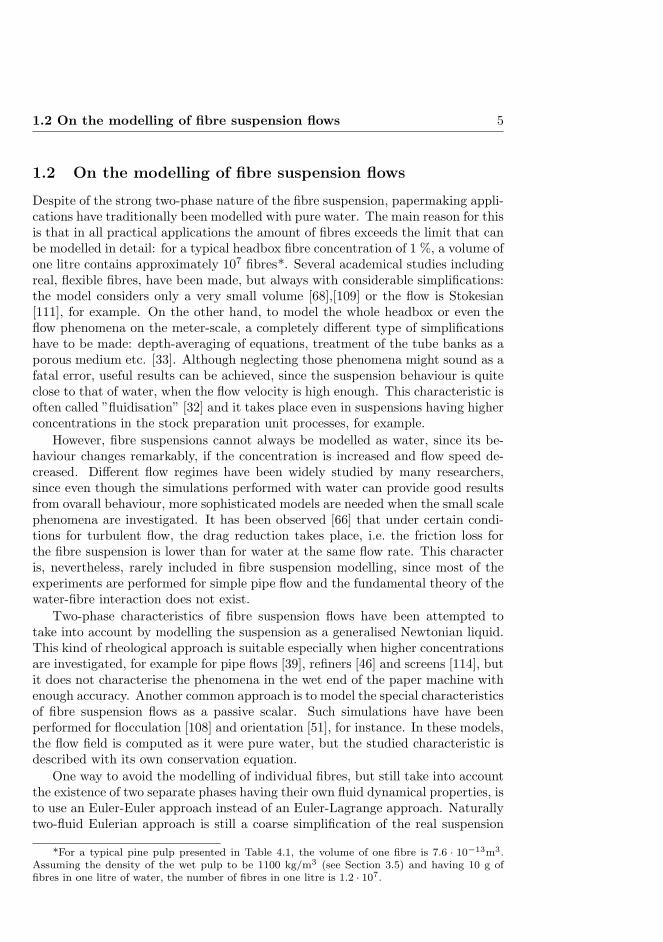
Despite of the strong two-phase nature of the fibre suspension, papermaking appli-cations have traditionally been modelled with pure water. The main reason for thisis that in all practical applications the amount of fibres exceeds the limit that canbe modelled in detail: for a typical headbox fibre concentration of 1 %, a volume ofone litre contains approximately 107 fibres*. Several academical studies includingreal, flexible fibres, have been made, but always with considerable simplifications:the model considers only a very small volume [68],[109] or the flow is Stokesian[111], for example. On the other hand, to model the whole headbox or even theflow phenomena on the meter-scale, a completely different type of simplificationshave to be made: depth-averaging of equations, treatment of the tube banks as aporous medium etc. [33]. Although neglecting those phenomena might sound as afatal error, useful results can be achieved, since the suspension behaviour is quiteclose to that of water, when the flow velocity is high enough. This characteristic isoften called ”fluidisation” [32] and it takes place even in suspensions having higherconcentrations in the stock preparation unit processes, for example.
However, fibre suspensions cannot always be modelled as water, since its be-haviour changes remarkably, if the concentration is increased and flow speed de-creased. Different flow regimes have been widely studied by many researchers,since even though the simulations performed with water can provide good resultsfrom ovarall behaviour, more sophisticated models are needed when the small scalephenomena are investigated. It has been observed [66] that under certain condi-tions for turbulent flow, the drag reduction takes place, i.e. the friction loss forthe fibre suspension is lower than for water at the same flow rate. This characteris, nevertheless, rarely included in fibre suspension modelling, since most of theexperiments are performed for simple pipe flow and the fundamental theory of thewater-fibre interaction does not exist.
Two-phase characteristics of fibre suspension flows have been attempted totake into account by modelling the suspension as a generalised Newtonian liquid.This kind of rheological approach is suitable especially when higher concentrationsare investigated, for example for pipe flows [39], refiners [46] and screens [114], butit does not characterise the phenomena in the wet end of the paper machine withenough accuracy. Another common approach is to model the special characteristicsof fibre suspension flows as a passive scalar. Such simulations have have beenperformed for flocculation [108] and orientation [51], for instance. In these models,the flow field is computed as it were pure water, but the studied characteristic isdescribed with its own conservation equation.
One way to avoid the modelling of individual fibres, but still take into accountthe existence of two separate phases having their own fluid dynamical properties, isto use an Euler-Euler approach instead of an Euler-Lagrange approach. Naturallytwo-fluid Eulerian approach is still a coarse simplification of the real suspension
*For a typical pine pulp presented in Table 4.1, the volume of one fibre is 7.6 · 10−13m3.Assuming the density of the wet pulp to be 1100 kg/m3 (see Section 3.5) and having 10 g offibres in one litre of water, the number of fibres in one litre is 1.2 · 107.

6 1. Introduction
flow, but at least it enables the variation in the local concentration and investiga-tion of both of the phases separately. The separation of the phases is undoubtlyimportant to include in modelling of certain unit-processes, e.g. web forming [40],since most of the phenomena depend greatly on local concentration.
This cut-through presented the simulation approaches very shortly, since themodelling of fibre suspension flows is such a wide research area. The themes morecloser related to this thesis, fibre orientation, fibre flocculation and dewatering,are discussed more profoundly in Chapter 2.
1.3 Motivation and objectives for the thesis
The motivation for this thesis is derived from the real challenges to improve theunderstanding of the effect of headbox and forming section fluid dynamics on thepaper sheet forming. In all simulated geometries, the focus has been on modellingreal-life problems instead of making crucial simplifications of modelled mecha-nisms. Therefore, fibre orientation and fibre flocculation, as well as the free jetand dewatering are all included in this thesis, as together they determine the basicstructure of the paper produced.
In addition, one goal has been the development of new tools for the fibre sus-pension flow simulations. These tools are based on a commercial CFD, where allthe models used have been implemented in. Many special characteristics, suchas orientation, have previously been modelled with in-house codes developed byresearchers, since special models are often not easy to implement in commercialcodes. These in-house codes are, however, usually imposible to use by any otherthan the developer himself, and they are rarely connectable to modelling of otherphenomena. In addition, the two-way coupling is slow and complicated to perform,if the flow field is first solved in one software, and the resulting field is used in sim-ulation of the orientation, for example, in the other software. Using a commercialCFD sofware, by contrast, offers the possibility to create dependencies between allthe modelled mechanisms in one software, and it is relatively easy for others tocontinue the work of one reseacher.
Finally, the author has had in her mind the development of the new basisfor fibre suspension flow research. This basis lies on the two-phase modelling,and including as much physics and real phenomena in the simulation as possible.As mentioned in the previous section, fibre suspension flows are rarely modelledwith two-phase approach, as long as real unit-processes are investigated. This is,however, the future trend, since the computing capacity has been continuously in-creasing and the experiments provide more and more detailed information for thedevelopment of the fundamental theory and for the model validation. Moreover,very often the simulated situation is simplified so much that is has nearly nothingto do with the real-world phenomena. That kind of research is naturally valuable,when studying the micro-scale phenomena and developing new physical theories,but for the industrial challenges it does not have a lot to give. The purpose of thisreseach has been to reveal the mechanisms - and challenges - related to flocculationand sheet forming, and create a novel modelling approach to be further developed

1.4 Related publications 7
to describe the flocculation phenomena in more and more detail.
The concrete objectives of the thesis are
• to develop CFD tools suitable for industrial-scale simulations
• to develop fibre suspension flow modelling based on the Eulerian multi-phaseapproach instead of commonly used one-phase flow or rheological approxi-mations
• to extend the solution of the fibre orientation probablity distribution (FOPD)model from mathematically one-dimensional form to two-dimensional one,and to predict fibre orientation in the headbox jet
• to bring new modelling approach to the pulp and paper industry for the me-chanical fibre flocculation modelling to replace a more abstract flocculationindex of the 20 years old Steen’s model
• to predict concrete floc size distributions and evolution of the floc size bymeans of CFD
• to study the influence of the jet-to-wire speed ratio to resulting fibre flocevolution in the initial drainage zone
1.4 Related publications
Part of the research presented in this thesis has also been published in journal andconference papers. The following papers are directly related to this work:
• Hamalainen, T., Hamalainen, J., Modelling of fibre orientation in the headboxjet, Journal of Pulp and Paper Science, Vol. 33 (1), pp.49-53, 2007
• Hamalainen, T., Hamalainen, J., Salmela, J., Evolution of Fibre Flocs in aTurbulent Pipe Expansion Flow, in proceedings of 6th International Confer-ence on Multiphase Flow, ICMF’07, Leipzig, Germany, 2007
• Hamalainen, T., Hamalainen, J., Korpijarvi, J., Prediction of the Sheet For-mation Using the Fibre Floc Evolution Model, in proceedings of PaperCon’08 - TAPPI/PIMA/Coating Conference, 2008
In all the three papers mentioned above, the modelling and the implementation,as well as analysing the results, were carried out by the author of this thesis underthe guidance of Jari Hamalainen. For the second paper the experimental data wasproduced by Juha Salmela and for the third paper the simulated geometry wasprovided by Jarmo Korpijarvi, but all the theoretical and computational work wasdone by the author of this thesis.
In addition, the following publications has been refered to:

8 1. Introduction
• Hamalainen, J., Hamalainen, T., Madetoja, E., Ruotsalainen, H., CFD-basedOptimization for a Complete Industrial Process: Papermaking, in ”Optimiza-tion based on Computational Fluid Dynamics”, Eds. D. Thevenin and G.Janiga, Springer, 2008
• Niskanen, H., Hamalainen, T., Eloranta, H., Vaittinen, J., Hamalainen, J.,Dependence of fibre orientation on turbulence of the headbox flow, 94th An-nual Meeting of Pulp and Paper Technical Association of Canada, pp. B339-B342, 2008
The first mentioned does not directly relate to the subject of this thesis, but itprovided a possibility for assuring the reliability of the CFD in the slice channel.The contribution of the author of this thesis in the mentioned book chapter consistsof modelling the pilot-scale-sized slice channel for the comparison with HOCS Fibresimulator. The most of the simulations presented in, and also the ideas behindthe chapter were contribution from Jari Hamalainen. Elina Madetoja and HenriRuotsalainen provided the examples for the optimisation and decission-supportcases. For the second publication, that is, the conference paper by Niskanen et al.,the author of this thesis has been a member of the supervising group. Althoughthe paper has been referenced in this thesis, the results are not included, sincethey will be part of doctoral thesis of Heidi Niskanen.
Finally, there are two more papers, which are not referenced in this thesis,since they are to be submitted:
• Hamalainen, T., Hamalainen, J., Modelling the Flocculation with Fibre FlocEvolution Model, to be submitted
• Hamalainen, T., Hamalainen, J., Modelling the Influence of the Jet-to-WireRatio to Resulting Fibre Floc Evolution in the Initial Drainage Zone, to besubmitted
The above papers contain mainly the same results presented in this thesis, andthe contribution of the author of this thesis is the modelling and the implementa-tion, as well as analysing the results under the guidance of Jari Hamalainen.

Chapter 2
Special characteristics of fibre suspension flows
Since the detailed modelling of fibre suspensions is not possible in practical ap-plications, suspensions are often tried to describe by simulating separately thespecial characteristic of intrest. Every special characteristic needs specified mod-elling method; orientation, flocculation and dewatering have to be connected tothe local flow field and turbulence in different ways. The following three subsec-tions give a brief view about the nature of the named characteristics, but firstlysome common terms, which often cause confusion, are explained.
In this thesis, the terms formation and forming are used as definined also byNorman and Soderberg in their extensive review of forming literature [83]: theterm formation exclusively refers to the small-scale basis weight variation of theready paper sheet (or the paper web in the forming section) and the term forming,for one, covers the process of producing the paper web in the forming section.In addition, following the practise introduced in [83], the term ”consistency” isavoided, and the use of term concentration is prefered. Although the term ”con-sistency” is widely used in the pulp and paper industry for the pulp concentration,it may cause misunderstanding, since the word has also other meanings.
Nonetheless, regarding the terminology of fibre orientation, slightly differentutilisation compared to [83] is applied. The term orientation is used both for theoverall process of orientation of fibres and the orientated state of the suspension. Inaddition, the term fibre orientation angle is often employed for the fibre orientationmisalignment. Similarly, the utilisation of the term flocculation differs from theone proposed in [83], where flocculation could mean both the aggregated stateof the suspension and the process of fibres attaching into a floc. In this thesis,the term flocculation is exclusively reserved for the dynamic overall process, inwhich the flocs coalesce and break-up. As regards to the aggregated state of thesuspension, it is chosen to use the term flocculated state of the suspension.
9

10 2. Special characteristics of fibre suspension flows
2.1 Fibre orientation
Fibre orientation is often considered simply as a misalignment angle with respectto the machine direction (MD), having a profile in the cross machine direction(CD). Modelling and optimization of the CD profile of the fibre orientation angle ispresented in [36], where the orientation is modelled based on the MD/CD velocityratio together with the jet-to-wire speed difference. The model gives surprisinglygood results when applied to cross-directional fibre orientation profile control,but when investigating the forming of the paper structure, a more comprehensiveapproach is needed.
Large scale phenomena, such as curling of a paper sheet, can be predicted withacceptable accuracy using only the described simple model, but predicting smallscale phenomena, such as cockling and fluting, requires information of local fibreorientation distribution. Simple models assume that there is only one fibre at eachposition, but to be precise, in any location (or, in a small volume) there are plentyof fibres oriented more or less randomly in different directions, thus forming adistribution of fibre orientation angles.
The fibre orientation probability distribution, ψ, can be presented as a statis-tical function or as a so-called ”orientation ellipse” (see Fig. 2.1). The orientationellipse provides the same information as the probability distribution, that is, themisalignment angle and the anisotropy. The angle θ shows the direction in whichthe most of the fibres are oriented and the anisotropy (i.e. the ratio between theaxes of ellipse) describes the magnitude of unequal orientation, in other words, thevariance.
Figure 2.1: Correspondence of fibre orientation distribution and the orientation
ellipse.
The importance of fibre orientation in the structure of the paper sheet has beenextensively reviewed in [79] and the effects of its z-directional variation have been

2.2 Fibre flocculation 11
studied in [67]. The measurement of the orientation is usually performed for theready paper, and the most commonly used method is the tape splitting, in whichthe paper sample is splitted into several layers, see [24], for example. The onlinemeasurement techniques in papermachine are described in [101]. To enhance fun-damental knowledge of the orientation in the wet end, several experimental studieshave been made for the orientation in the flowing suspension, see for example [13],[23] and [112].
The mathematical model for the fibre orientation distribution was originallyderived by Jeffery in early 1920’s [53]. He studied an ellipsoidal particle moving in aStokes flow, assuming an inertialess particle and a constant fluid velocity gradient.The theory is later extended to more complex shear flows; see for example [102].During the recent years, the fibre orientation model has actively been studied forpulp and paper industrial applications by Olson and co-authors, for example, [84],[85], [86]. For an extended review of different geometries, see Hyensjo [48].
One disadvantage in the orientation distribution model is that it is quite dif-ficult and costly to solve (more discussion can be found in Section 3.2). Hence,there exist other approaches to overcome these difficulties, and one of them is theorientation tensor approach, used by Advani and Tucker [2], among others. Inthe orientation tensor method the distribution is described with even-order ten-sors. However, this procedure leads to other problems: one has to define a closureequation to obtain resolvable system of equations.
The fibre orientation is mostly modelled as a passive scalar, since the detailedmodelling would require the simulation of real, flexible fibres and their interactions,which cannot be afforded in the industrial scale. Therefore, a one-phase modellingapproach is usually sufficient for orientation studies in practical applications. Asa consequence, neglecting the fibre-fibre interactions signifies that the suspensionis assumed very dilute. However, all the performed experiments for the fibreorientation are also made for dilute suspensions, since distinguishing a single fibreis not possible even for concentrations used typically in headboxes, see [12], [23]and [112], for example.
2.2 Fibre flocculation
The flocculation of a suspension is determined by its uniformity and mobility offibres [60]. It has been suggested in [104], that the interfibre contact is a key factorin flocculation, since it has a straightforward effect on the two named properties.In papermaking process, plenty of chemicals are added in the fibre-water suspen-sion in order to enhance and strenghten the interfibre contacts. However, fibreflocculation is known to occur primarily from mechanical interaction between fi-bres [72]. It has been shown also by simulations [100] that fibres flocculate withoutattractive forces and that the floc formation occurs through an elastic interlockingmechanism. Fibre-fibre interaction becomes important when a certain critical con-centration is exceeded. Mason [72] suggested this condition to be as one in whichthere is less than one fibre in a volume having a diameter equal to the length ofa single fibre. In practical papermaking concentrations this value is always sur-

12 2. Special characteristics of fibre suspension flows
passed, and hence, the interaction has to be taken into account. In addition, thebehaviour of the fibrous phase depends significantly of the type of fibre contact.In order to characterise the behaviour of different pulps, Kerekes and Schell [60]have defined a parameter called crowding factor:
Ncf =23cv
(LfDf
)2
(2.1)
where cv denotes volumetric fibre concentration, Lf average fibre length and Df
average fibre diameter. The crowding factor represents the number of fibres withinthe rotational sphere of influence of a single fibre, see illustration in Fig. 2.2, wherethe crowding factor is 6.
Figure 2.2: Schematic characterisation of the definition of crowding factor.
In many references, see e.g. [60], the crowding factor is represented by meansof mass concentration of fibres, cm, and fibre coarseness, ωf , giving the form
Nmf ≈5cmL2
f
ωf(2.2)
It should be noted, however, that this notation is rather misleading, since it doesnot provide a dimensionless number like the Eq. (2.1), but has units of [m3/kg], ifthe procedure recommended in [60] is used; to obtain the right order of magnitude,the value of concetration has to be expressed in %. If these inconveniences areexcluded, the values of Eqs. (2.1) and (2.2) agree relatively well: for a given pulpused later in numerical examples Ncf gives the value of 116 and Nmf the value of102. As a matter of fact, several corrections, e.g. [45] and [63], to the definitionof crowding factor have been proposed, which indicates that the concept of thecrowding factor has recieved considerable interest, but on the other hand, is notvery well established. Therefore, the special attention has always to be paid whenusing this dimensionless number. In this thesis, the definition of Eq. (2.2) isexclusively used.

2.2 Fibre flocculation 13
Kerekes and Schell suggested that crowding factor could be a useful tool forcharacterising the flocculation potential of different pulps [60]. They have usedcrowding factor to classify fibre suspensions into three different regimes perceivedalso by Soszynski [107], see Table 2.1. When the crowding factor is less than 1, fibresuspension is in dilute regime, which is characterised by chance of collision. Forcedcollisions appear when the crowding factor is between 1 and 60* ; this regime iscalled semi-concentrated. For values greater than 60, the fibre suspension is inconcentrated regime, which is characterised by continuous contact between fibres.
Table 2.1: Characterisation of fibre suspension regimes by means of crowding
factor
Regimes Type of fibre contact Crowding factor, NfDilute Chance collision Nf < 1
Semi-concentrated Forced collision 1 < Nf < 60∗
Concentrated Continuous contact Nf > 60∗
The crowding factor has been agreed to characterise the fibre flocculation phe-nomenon by several authors, Kerekes and Schell [61], among many others, butits utilisation in modelling has been limited to simple expressions for so-calledflocculation index [45]. Or, the flocculation tendency of different pulps has beenestimated by experimental methods in order to determine some guidelines forcontrolling the paper properties, see for example [20] or [21]. The approach isestablished on number of contacts per fibre and connected to flow conditions bysimple equations. Although these approximations are still far from being able topredict the flocculated state of fibre suspension in real papermaking environment,they provide very useful knowledge of behaviour of fibre suspensions. Farnoodet al. [26] have also presented a theoretical model for the intra-floc forces, but itis derived for simple model flocs containing only couples of fibres, and has notbeen used in any real-scale studies. Totally another type of approach is presentedby Hourani [44], whose model is based on the mass-action law and the energyspectrum of turbulent flow. However, the model still contains parameters whichdetermination is not straightforward, and hence, one cannot talk about an overallmodel to be used widely in industrial applications.
To the author’s knowledge, the flocculation model the most used at the indus-trial scale applications is the one proposed by Steen [108]. Steen’s model treats thefibre suspension as one-phase flow, and the flocculation phenomenon is describedby the concentration variations solved as a passive scalar. He defined a conceptcalled flocculation intensity, which describes the concentration fluctuation of theimagined fibrous phase. Steen’s model has been compared to experimental results
*The upper value is defined by apparition of coherent flocs, which has been observed tooccur for crowding factors between 60 and 130, depending on the local flow conditions. For moredetailed discussion see [60].

14 2. Special characteristics of fibre suspension flows
by many researchers, Hyensjo among others [50], whose reference data was pro-duced by Karema et al. [57]. It has been shown in [50] that Steen’s model is ableto capture the tendencies at some level, if the model parameters are adequatelytuned, but it is still far away from predicting the flocculated state of the suspen-sion. Kuhn and Sullivan [64] and Plikas et al. [90] used similar approach of scalarfluctuation as Steen has presented. However, the model parameters were cali-brated with the experimental data obtained by Raghem-Moayed [94], and hence,the model is applicable only for flows where grid-generated turbulence dominates.In addition, no matter how well the model parameters are tuned, the scalar ap-proach always neglects the real physical two phase nature of fibre suspensions, andfor example, real concentration variations cannot be investigated. Moreover, theflocculation intensity is an intangible concept, which is difficult to connect to thereal behaviour of flocs, especially to the incidence of different floc sizes.
Although the modelling of the flocculation has not been a very active area ofresearch, there exists a great amount of experimental work. Floc formation anddisruption in several kinds of flows has widely been studied by many authors: forfloc formation in decaying turbulence, see [58] and [95], and for floc break-up inextensional flows, see [59] and [52], just to mention few. Based on these studies,one can define some geometry-dependent correlations, which may be very usefulin improving certain unit-processes in papermaking, but still the fundamentalknowledge of floc break-up and coalescence mechanisms is lacking. There is, thus, areal need for more detailed experiments, which could reveal the connection betweenflocculation and small-scale flow phenomena.
2.3 Dewatering and paper web forming
Although the fluid dynamics in the headbox affect greatly the quality of the paperproduced, the basic structure is determined during the forming process. Afterthe forming section, only fines and fillers can move towards the surfaces duringpressing, but the fibres stay in positions they have taken during the forming.
The modelling of forming includes first of all the modelling of free jet, since thejet contraction and the jet angle depend on the slice opening and the bottom lipextension, for example. Soderberg carried out both experimental and theoreticalstudies of planar liquid jets [105]. He assumed incompressible Newtonian fluidsand laminar flows, and derived the model to solve the jet position based on theforce balance of the jet following general free-boundary theories. The jet shapewas solved based on a potential flow model. The Reynolds numbers were 1000and 10000, when for a typical jet it should be around 300000 (the slice opening ≈1 cm and the jet speed ≈ 1800 m/min). A more advanced approach is presentedby Niemisto et al. in [76], where the flow is turbulent and modelled with thek − ε model. In their work the position of the free surface was solved numericallywithout the surrounding gas, i.e. iterated with the help of the kinematic conditionu · n = 0, where u is velocity and n is the outward unit vector of the free surface.With today’s commercial CFD softwares the modelling of free jet is, nevertheless,quite a routine task, but requires remarkable computer capacity, and is still fairly

2.3 Dewatering and paper web forming 15
challeging, if some special characters, such as flocculation, for exemple, is includedin the model. In many practical applications, a simple, approximative solutionis accurate enough, and hence, one can rely, for instance, on Tappi TechnicalInformation Sheet (TIS), where the determination of the jet contraction and theangle is based on inviscid equations (potential flow). In addition, several authors,see e.g. [48], have studied different phenomena in the free jet by using a fixed jet,i.e. a straight channel with slip boundary conditions.
In order to predict the forming of the paper produced, one should include theeffects of different dewatering components (forming roll, loadable blades, vacuumroll etc.) in the forming section, but also the dewatering and the consolidationphenomena. Modelling the jet impingement and the initial drainage zone has beenthe objective of many recent studies. Audenis and Dahkild examined the impinge-ment of an inviscid jet on a single fabric [5], while Dalpke and her co-authorshave published several studies for a twin-wire machine in order to enhance theknowledge on phenomena in the initial drainage and the fibre mat build-up, seee.g. [15] and [17]. In order to investigate the hydrodynamical forces and hydrody-namical shear at the vicinity of the forming fibre mat, Deng and Martinez haveperformed an experimental and theoretical study with a channel partially filledwith the porous medium [18]. The pressure pulse on wires has been investigatedcomputationally by Audenis [4], where also the wire porosity is included in themodel. Experimental studies for the pressure pulsation have been carried out withKTH-former by Holm [42] and Bergstrom [10], who examined also the floc elonga-tion and breakage during the roll forming for different jet-to-wire ratios. The wireposition and pressure distribution due to the loadable blades have earlier beenstudied by Zhao and Kerekes [119] and by Zahrai [118].
The simulation of the fibre retention has not been such a popular area ofresearch as the other phenomena on the drainage zone, but some studies on theinitial fibre retention have been made, see for example [7]. In most of the studies,see e.g. [17], the retention has been assumed 100%, and the attention has beenpaid on other issues. Also, the dewatering process has widely been treated as apurely filtration process, and the web consolidation has been taken into accountonly in few studies, see for example Hiltunen [40].
As can be imagined based on the research briefly described above, the predic-tion of formation is highly complex issue, and it is not always straightforwardlyconnectable to flocculated state of a given suspension. The superposition of flocsand fibres upon one another on a moving wire may induce different level of unifor-mity on the web compared to the state in flowing suspension. It has been shownin [30], that superposition of flocs of low density improves the formation. On theother hand, the role of concentration is not that simple: Smith showed that thedrainage conditions together with pulp concentration affect the resulting forma-tion [104], and so does the fibre length as well [55]. Moreover, the mobility offibres in a flowing suspension is an important property for the resulting formation,as shown by Martinez et al. [71]. They studied different suspensions in laboratoryand papermachine scale and found a correlation between a critical crowding factor,yield stress and good formation.

16 2. Special characteristics of fibre suspension flows
Although several studies are entitled to give an impression that the formationis predicted based on the flocculated state of the suspension, the experimental andnumerical studies really including that kind of investigation, are still rare. Onesuch a study is presented by Dodson and Serafino [22], who attempted to modelthe formation resulting from a random distribution of flocs dispersed in the fibresuspension entering the wire section. Some other papers have been published aswell, but usually the flocs are described with some idealistic configuration called”model flocs”, meaning that a floc contains only few fibres and has a form of a star[19] or a disc [25] [27]. Therefore, these approaches are not utilisable in predictingthe real formation based on the flocculated state, and they have been critisisedalso by producing unrealistic floc grammage levels [81].
One special property in web forming is the self-healing effect. It has beennoticed that the fibre distribution in a ready paper sheet is more even than wouldbe indicated by the flocculated state of the flowing suspension [80]. This is dueto the fact that if there is a hole in the forming paper web during the dewateringprocess, the local dewatering resistance is lower than in other areas, and hence,the free suspension will be dewatered in that position and carry the free fibresthere as well. This phenomenon is also called ”hydrodynamic smoothing”, and ithas been noticed to vary depending on range of basis weight and crowding factor[98]. The results of Norman [80] confirmed that for small and medium floc sizesthe real sheet is more even than the random sheet, but for larger flocs the sheetis, nevertheless, more uneven. Although the experimental work indicates that theeffect of fibre mat resistance to the local forming is not always straightforward, itis, however, obvious, that the effect of already formed web should be included insimulations, such as Zahrai, for example, has done [118].

Chapter 3
Mathematical models
In the following sections the modelling approaches used in this thesis are presented.As already mentioned in Section 2.1, the fibre orientation can be modelled withone-phase flow approach, and hence, those equations are presented at first. Theflocculation is modelled with a totally novel approach in pulp and paper industry,and therefore, the equations and theory behind them are comprehensively reportedin Section 3.5. Since the modelling of flocculation requires the two-phase approach,the whole Eulerian two-phase equations are introduced in Section 3.3. In addition,the modelling of turbulence in fibre suspension flows is briefly reviewed in Section3.4, since it has received a considerable attention during recent years, and is stilla subject to debate. The last part of this chapter, Section 3.6, goes through theissues concerning the dewatering model used in this thesis.
3.1 Governing equations for one-phase flow
For the incompressible fluids, the stady-state continuity equation can be writtenas:
∂
∂xi(ρcuc,i) = 0 (3.1)
where uc,i are time-averaged velocity components in cartesian coordinates xi andρc denotes the density of the fluid. The index c refers to continuous fluid, andis used also for the one-phase flow equations in order to have congruent notationthroughout the thesis.
The momentum equation for the turbulent flow is:
∂
∂xj(ρcuc,iuc,j) = − ∂
∂xj(pδij) +
∂
∂xj(τc,ij) −
∂
∂xj
(ρcu
′c,iu
′c,j
)+Bc,i (3.2)
where p denotes pressure, δij stands for Kronecker delta and ρcu′ciu
′cj are Reynolds
stresses, the modelling of which will be briefly reviewed in Section 3.4. B represents
17
18 3. Mathematical models
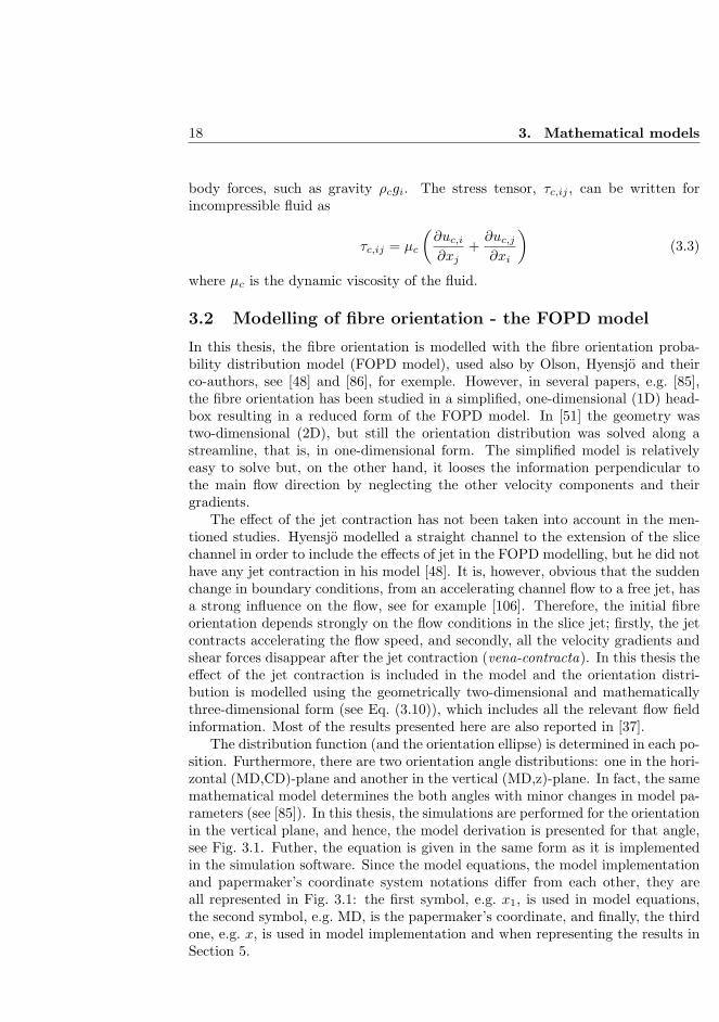
body forces, such as gravity ρcgi. The stress tensor, τc,ij , can be written forincompressible fluid as
τc,ij = µc
(∂uc,i∂xj
+∂uc,j∂xi
)(3.3)
where µc is the dynamic viscosity of the fluid.
3.2 Modelling of fibre orientation - the FOPD model
In this thesis, the fibre orientation is modelled with the fibre orientation proba-bility distribution model (FOPD model), used also by Olson, Hyensjo and theirco-authors, see [48] and [86], for exemple. However, in several papers, e.g. [85],the fibre orientation has been studied in a simplified, one-dimensional (1D) head-box resulting in a reduced form of the FOPD model. In [51] the geometry wastwo-dimensional (2D), but still the orientation distribution was solved along astreamline, that is, in one-dimensional form. The simplified model is relativelyeasy to solve but, on the other hand, it looses the information perpendicular tothe main flow direction by neglecting the other velocity components and theirgradients.
The effect of the jet contraction has not been taken into account in the men-tioned studies. Hyensjo modelled a straight channel to the extension of the slicechannel in order to include the effects of jet in the FOPD modelling, but he did nothave any jet contraction in his model [48]. It is, however, obvious that the suddenchange in boundary conditions, from an accelerating channel flow to a free jet, hasa strong influence on the flow, see for example [106]. Therefore, the initial fibreorientation depends strongly on the flow conditions in the slice jet; firstly, the jetcontracts accelerating the flow speed, and secondly, all the velocity gradients andshear forces disappear after the jet contraction (vena-contracta). In this thesis theeffect of the jet contraction is included in the model and the orientation distri-bution is modelled using the geometrically two-dimensional and mathematicallythree-dimensional form (see Eq. (3.10)), which includes all the relevant flow fieldinformation. Most of the results presented here are also reported in [37].
The distribution function (and the orientation ellipse) is determined in each po-sition. Furthermore, there are two orientation angle distributions: one in the hori-zontal (MD,CD)-plane and another in the vertical (MD,z)-plane. In fact, the samemathematical model determines the both angles with minor changes in model pa-rameters (see [85]). In this thesis, the simulations are performed for the orientationin the vertical plane, and hence, the model derivation is presented for that angle,see Fig. 3.1. Futher, the equation is given in the same form as it is implementedin the simulation software. Since the model equations, the model implementationand papermaker’s coordinate system notations differ from each other, they areall represented in Fig. 3.1: the first symbol, e.g. x1, is used in model equations,the second symbol, e.g. MD, is the papermaker’s coordinate, and finally, the thirdone, e.g. x, is used in model implementation and when representing the results inSection 5.

3.2 Modelling of fibre orientation - the FOPD model 19
Figure 3.1: Orientation angles in spherical coordinates [77].
The FOPD equation is based on the planar approach of the Fokker-Planckequation:
Dψ
Dt−Dt
∂2ψ
∂x2i
= − ∂
∂φ
(ψφ)
(3.4)
where ψ(t, xi, φ) denotes the fibre orientation probability distribution, φ is the fibreorientation angle in position xi at time t, Dt the translational diffusion coefficientand φ the time rate of change of the orientation vector of an ellipsoid of revolution[3]. Based on Jeffery [53] φ can be written
φ = −Dr
ψ
∂ψ
∂φ− 1
2sin (2φ)
∂u1
∂x1− sin2 φ
∂u1
∂x2+ cos2 φ
∂u2
∂x1+
12
sin (2φ)∂u2
∂x2(3.5)
where Dr is the rotational diffusion coefficient. Eq. (3.5) is valid for fibres havinginfinite lenght-to-diameter aspect ratio, that is, for relatively long fibres, see Olsonand Kerekes [86]. It has been numerically tested that for fibres used in pulp andpaper industry, this simplification does not violate the results; the aspect ratioshould be below 10 before any modification in the orientating behaviour could beseen, and thus, this simplification is justified.
Using Eq. (3.5) the right hand side of Eq. (3.4) can be written
− ∂
∂φ
(ψφ)
=− ∂
∂φ
(−ψDr
ψ
∂ψ
∂φ
)− ∂
∂φ
(−ψ 1
2sin (2φ)
∂u1
∂x1
)− ∂
∂φ
((−ψ sin2 φ
) ∂u1
∂x2
)− ∂
∂φ
((ψ cos2 φ
) ∂u2
∂x1
)− ∂
∂φ
(ψ
12
sin (2φ)∂u2
∂x2
) (3.6)

20 3. Mathematical models
Since Dr and velocity gradients do not depend on φ, the equation can be reorgan-ised as follows:
− ∂
∂φ
(ψφ)
=Dr∂2ψ
∂φ2+
∂
∂φ
(ψ
12
sin (2φ))
︸ ︷︷ ︸(1)
∂u1
∂x1+
∂
∂φ
(ψ sin2 φ
)︸ ︷︷ ︸
(2)
∂u1
∂x2
− ∂
∂φ
(ψ cos2 φ
)︸ ︷︷ ︸
(3)
∂u2
∂x1− ∂
∂φ
(ψ
12
sin (2φ))
︸ ︷︷ ︸(4)
∂u2
∂x2
(3.7)
The derivatives for the terms denoted with (1), (2), (3) and (4) can be expressed
(1)∂
∂φ
(ψ
12
sin (2φ))
=∂ψ
∂φ
12
sin (2φ) + ψ∂
∂φ
(12
sin (2φ))
=(
12
sin (2φ))∂ψ
∂φ+ (cos (2φ))ψ
(2)∂
∂φ
(ψ sin2 φ
)=∂ψ
∂φsin2 φ+ ψ
∂
∂φ
(sin2 φ
)=(sin2 φ
) ∂ψ∂φ
+ (sin (2φ))ψ
(3) − ∂
∂φ
(ψ cos2 φ
)= −∂ψ
∂φcos2 φ− ψ ∂
∂φ
(cos2 φ
)= −
(cos2φ
) ∂ψ∂φ
+ (sin (2φ))ψ
(4) − ∂
∂φ
(ψ
12
sin (2φ))
= −∂ψ∂φ
12
sin (2φ)− ψ ∂
∂φ
(12
sin (2φ))
=(
12
sin (2φ))∂ψ
∂φ+ (− cos (2φ))ψ
(3.8)
Substituting the derivatives in Eq. (3.6) gives:
− ∂
∂φ
(ψφ)
= Dr∂2ψ
∂φ2
+[
12
sin (2φ)(∂u1
∂x1− ∂u2
∂x2
)+ sin2 φ
∂u1
∂x2− cos2 φ
∂u2
∂x1
]︸ ︷︷ ︸
C
∂ψ
∂φ
+[cos (2φ)
(∂u1
∂x1− ∂u2
∂x2
)+ sin (2φ)
(∂u1
∂x2− ∂u2
∂x1
)]︸ ︷︷ ︸
R
ψ
(3.9)

3.3 Eulerian two-fluid model 21
Using the above notations C and R, and suppressing the time derivative, Eq. (3.4)becomes:
−Dt∂2ψ
∂xi∂xi−Dr
∂2ψ
∂φ2+
∂
∂xi(uiψ) = C
∂ψ
∂φ+Rψ (3.10)
The unknown probability function ψ(x1, x2, φ) depends on the geometrical posi-tion (x1, x2) and on the angle φ. Hence, it leads to a non-standard geometricalmodelling, that is, when geometry is two-dimensional, the FOPD model is three-dimensional. The section 4.1 introduces in more detail, how the dimensions arehandled in the model, and describes also the boundary conditions used.
One shortcoming of the FOPD model is that it is derived for dilute suspen-sions. This means that fibre-fibre interactions are not taken into account. Thisis somehow quite a serious drawback, since, as mentioned before, in all practicalpapermaking applications, there are fibre-fibre connections. Krochak et al., forexample, showed that flocculation occurs even at low concentrations [62]. In addi-tion, in the current model, there is only one-way coupling between fluid dynamicsand the FOPD model, that is, fluid dynamics affect to fibre orientation, but notvice versa. The turbulence modification in the presence of fibres is largely recog-nised phenomenon, and it could quite easily be added in the model by modifyingthe source terms of turbulence equations. However, this is not accomplished, sincethe fundamental theory of this phenomenon does not exist, see Section 3.4 forfuther discussion. Despite of the mentioned deficiencies, the FOPD is, however,the best available model at present, and widely used by many reseaches, since itprovides, after all, very useful knowledge of fibre suspensions. It is worth to keepin mind that also the experiments investigating the fibre orientation are made fordilute suspensions, the concentration being ≈0.01%, i.e. even less than in whitewater. In addition, the tissue headboxes are typically run with the concentrationof ≈ 0.1%, and thus, in such applications the FOPD model might be able to fairlyaccurately predict the fibrous structure of the end product.
3.3 Eulerian two-fluid model
The Eulerian two-fluid model used in this thesis is based on the ”traditional” twocomponent forms of continuity and momentum equations, which can be found inany multiphase text book, see e.g. [14]. The equations presented here follow mainly[14] and are all formulated in the steady-state form. The two-fluid approach iscommonly accepted modelling method, and used by several researhers for air-fibreflows, see eg. [69] and [73]. In the Eulerian approach, the prescence of particlesin the flow is taken into account by modelling the particle phase as a separate,immiscible liquid, and the interactions between two phases are included in themomentum equations via drag and possible other forces. The governing equationsare averaged, and in each computational cell there is a certain volume fraction(even an infinitely small) of both flowing media. In this thesis, the equations areformulated for water and flocs, and hence, the material properties for floc phase are

22 3. Mathematical models
not the same as for fibres. Determining the floc phase properties is a complicatedissue, and it will be more closely discussed in Section 3.5.
The continuity equation for two-fluid flow can be written
∂
∂xi(αkρkuk,i) = Sk (3.11)
where the index k is c for continuous phase (here water) and d for dispersed phase(flocs). αk stands for the volume fraction, ρk for the density and uk for the velocity.Sk is the source term, which is, naturally, equal to zero, if no mass transfer betweenthe two fluids is present.
The momentum equation for the continuous phase can be written as:
∂
∂xj(αcρcuc,iuc,j) =− αc
∂
∂xj(pδij) +
∂
∂xj(αcτc,ij) + fcd (ud,i − uc,i)
− ∂
∂xj
(αcρcu
′c,iu
′c,j
)+Bc,i
(3.12)
and for the fibrous phase:
∂
∂xj(αdρdud,iud,j) =− αd
∂
∂xj(pδij) +
∂
∂xj(αdτd,ij) + fcd (uc,i − ud,i)
− ∂
∂xj
(αdρdu
′d,iu
′d,j
)+Bd,i + FSPd,i
(3.13)
where Bc,i and Bd,i are body forces, and FSPd,i represents additional interphasemomentum transfer to be added in certain circumstances, for example in the de-watering modelling, see Section 3.6. The terms fcd (ud,i − uc,i) and fcd (uc,i − ud,i)in Eqs. (3.12) and (3.13) represent the interphase drag between water and fibrousphase. The drag coefficient, fcd, can be written as:
fcd =Ccd8Acdρc |ud,i − uc,i| (3.14)
where Acd is the interfacial area density defined as Acd = 6αd/dave, where dave de-notes the mean diameter of spherical particles. The dimensionless drag coefficient,Ccd, is modelled with the Schiller-Naumann [99] correlation, which is commonlyused in dispersed particle flow simulations:
Ccd =
24Rer
(1 + 0.15 (Rer)
0.687)
if Rer < 1000
0.44 if Rer > 1000(3.15)
where Rer is the relative Reynolds number based on the relative speed betweencontinuous and dispersed phase, Rer = ρcdave |uc,i − ud,i| /µc. For single fibres,there exist models for drag coefficients, but they are not suitable for flocs, since

3.4 Modelling of turbulence 23
flocs can be assumed quasi-spherical, except in strogly elongational flows. In ad-dition, there are no better assumptions available for the fibre floc drag, and hence,the Schiller-Naumann correlation is chosen.
3.4 Modelling of turbulence
Turbulence modification in presence of particles is well-recognised, but still in-adequately known phenomenon. Several authors have used the modified k − εmodel based on [92]. The model includes the additional dissipation caused by theprescence of particles, but neglects the additional production due to the particles.Although in some fluid-particle flows the supplementary production is important[69], in the modelling of flocculation in fibre-water suspensions it can be neglected,since wake production does not occur. The dampening of turbulence is not, how-ever, such straightforward phenomenon. It has been shown by many authors, e.g.[28] and [116], that fibres and flocs reduce turbulence intensity. For example,Norman and Soderberg suggested [83] that the prescence of fibres in a flow willsuppress those scales of the flow which are smaller than the fibre size. Benningtonand Thangavel [9] noticed that when fibre concentration is increased, more andmore energy was removed from the turbulence cascade. In addition, it is suggested[83] that fibres and flocs modify also the turbulence spectrum in such a way thatit is no longer continuous as it is for single-phase flows.
Nevertheless, the detailed measurement of turbulence in typical wet end con-centrations is not yet possible, and hence, no reliable theory about the turbulencedampening in fibre-water suspension is available. Therefore, in this thesis, the sim-ulations for the water phase are mostly performed with the standard k− ε model,without any modification of the source terms. One exception of this procedure isdone for the FOPD model in the slice channel, for which the Reynolds Stress Modelis applied. The reason for this is that in the slice channel turbulence is not at allisotropic [88], and it might probably have an effect on orientation. Nevertheless,for flocculation modelling an isotropic turbulence model is used, since it has beenthought that the uncertainty in the flocculation model does not specifically lie inturbulence modelling, but rather, in the definition of floc break-up and coalescencemechanisms.
In the k − ε model for the continuous phase the Reynolds stresses, ρcu′c,iu
′c,j ,
in Eq. (3.2) are modelled using the Boussinesq hypothesis:
−ρcu′c,iu
′c,j = µtc
(∂uc,i∂xj
+∂uc,j∂xi
)− 2
3δijρckc (3.16)
where kc is the turbulent kinetic energy of the continuous phase given by
kc =12u
′c,iu
′c,i (3.17)
and µtc is the turbulent (or eddy) viscosity for the carrier phase defined by
µtc = ρcCµk2c
εc(3.18)

24 3. Mathematical models
where Cµ =0.09 and εc is the turbulent kinetic energy dissipation. The transportequations for the turbulent kinetic energy, kc, and for the dissipation, εc, of thecontinuous phase can be written:
uc,i∂(αcρckc)
∂xi=
∂
∂xi
((µc +
µtcσk
)∂(αckc)∂xi
)+ αcPkc − αcρcεc (3.19)
uc,i∂(αcρcεc)
∂xi=
∂
∂xi
((µc +
µtcσε
)∂(αcεc)∂xi
)+ αcCε1Pkc
εckc
− αcρcCε2ε2ckc
(3.20)
where the model constants are: Cε1 =1.44, Cε2 =1.92, σk =1.0 and σε =1.3 [65].Pkc is the production of the turbulent kinetic energy by the mean velocity fieldgiven as
Pkc = µtc
(∂ui∂xj
+∂uj∂xi
)∂ui∂xj
(3.21)
As stated above, the Reynolds Stress Model is used for the FOPD simulation.The transport equation for Reynolds stresses can be found in any turbulence textbook, see e.g. [91], and is applied in the steady-state form [1]:
uc,l∂(ρcu
′c,iu
′c,j
)∂xl
= Pij + Rij +∂
∂xl
((µc +
23Csρc
k2c
εc
)∂u
′c,iu
′c,j
∂xl
)
− 23δijρcεc
(3.22)
where Pij is the production tensor given by
Pij = −ρc(u
′c,iu
′c,l
∂uj∂xl− u′
c,ju′c,l
∂ui∂xl
)(3.23)
and Rij is the pressure-strain correlation, defined as
Rij = Rij,1 + Rij,2 (3.24)
There exist several different propositions for Rij,1 and Rij,2, one of them being
Rij,1 =− ρcεcCs1aij
Rij,2 =− ρcCr2kcSij + ρcCr4kc
(aijSij + ajiSij −
23aij · Sijδij
)+ Cr5ρckc (aijΩji + ajiΩij)
(3.25)

3.5 Modelling of fibre flocculation - the FFE model 25
and the anisotropy, aij , the strain rate, Sij , and the vorticity, Ωij , are written as
aij =u
′c,iu
′c,j
kc− 2
3δij (3.26)
Sij =12
(∂ui∂xj
+∂uj∂xi
)(3.27)
Ωij =12
(∂ui∂xj− ∂uj∂xi
)(3.28)
Finally, the coefficients in Eqs. (3.22) and (3.25) are: Cs =0.22, Cs1 =1.8, Cr2 =0.8,Cr4 =0.6 and Cr5 =0.6.
For the fibrous phase, one cannot really speak about turbulence, but rathersome fluctuation. Therefore, only a simple algebraic model is applied, and it isgiven as follows [1]
µtd =µtcPrt
(3.29)
where Prt is the turbulent Prandtl number.
3.5 Modelling of fibre flocculation - the FFE model
The flocculation is modelled with a totally novel approach in pulp and paperindustry, the Fibre Floc Evolution (FFE) model. The suspension is modelled asa turbulent two phase flow, with water being the carrier phase and the flocs asthe dispersed phase. Since the modelling approach is Eulerian, the presence ofsingle fibres is neglected, and the floc phase is treated as an immiscible liquid,having its own properties. Even though flocs are small fibre networks, which havea mechanical strength, they can be treated as a continuum, as far as the micro-scale phenomena are not taken into account. In addition, it must be emphasisedthat the properties of flocs are different from those of single fibres, and naturally,different from those of water.
In order to describe the physical behaviour of flocs, the fibrous phase is dividedinto several size groups, each of them representing different floc size. The modelis based on the population balance method, and thus, it provides detailed infor-mation of the floc size evolution. Flocs can coalesce into larger flocs or break-upinto smaller ones, which means that the basic flocculation dynamics is taken intoaccount. It is recognised that in real processes fibres can detach from a floc bysome kind of erosion mechanism, or, a single fibre can attach to a floc, and hence,modify the local floc size distribution. However, these mechanisms are not im-plemented into the FFE model, since any experimental data for such a validationdoes not exist, and modelling the effects mentioned would be very complicated.
The population balance method, as well as break-up and coalescence modelsused, are commonly known methods, and therefore, they are only briefly presented

26 3. Mathematical models
in next three subsections. The break-up phenomenon is modelled using Luo andSvendsen model [70] and the coalescence with Prince and Blanch model [93]. Bothmodels are based on the theories of isotropic turbulence and on the assumptionthat the particle size can be modified by eddies having length scale equal to orsmaller than the particle. The mentioned models are derived for spherical particles,such as bubbles. It has also been assumed that particles do not consist of smallercomponents in the same way as flocs consist of fibres. Therefore, the smallestmodelled unit refering to particle, is floc, in this thesis. Thus, it is worth to keepin mind that when presenting the break-up and coalescence models in Subsections3.5.2 and 3.5.3 the word ”particle” refers to floc.
Although the flocculation has been an active area of research for decades, itis still a matter of debate, which is the mechanism that causes the break-up andcoalescence of flocs. As early as 1979, Wahren stated that floc dispersion andaggregation are competing effects both promoted by turbulence [113]. Also Yoko-gawa et al. found a direct relation between the increased turbulence intencity andmore uniform suspension when studying the effects of various turbulence genera-tors [117]. Nevertheless, some researches have disagreed with these observationsand proposed that floc dispersion occurs due to the elongational flows, i.e. due tothe strain [82]. However, it has been proven by pilot-scale tests that the flocs breakup most efficiently in the tube expansion of the turbulence generator [57] wherethe increase of the turbulent kinetic energy can be observed, while the elongationdue to contractions is often able only to stretch the floc, which recovers its quasi-spherical shape after the elongation ceases [59]. In addition, it is commonly knownfact that the relatively calm flow in the slice channel is capable only to maintainthe floc size obtained in the turbulence generator, not to further break up the flocs[103]. It is, therefore, an appropriate approach to use the Luo and Svendsen modelfor the break-up and the Prince and Blanch model for coalescence, since both arebased on theories leaning on turbulence contribution in particle size modification.
In addition, the viscosity of fibre suspension flows has been the objective ofmany studies. Head loss (wall friction and apparent viscosity, as well) in longtubes of pulp-water mixture flows have been studied by Brecht and Heller [11], forexample, and it is known to vary significantly depending on the pulp concentration,fibre properties etc. The viscosity has been modelled as a generalized Newtonianfluid following the Power-Law model by Myreen [75] or as a Bingham fluid byWikstrom [114], for example. However, these studies are not directly applicable totwo-phase flow modelling, since they are treating the flowing media as a one-phaseflow. In other words, the suspension is assumed homogenious having one viscositydependent on shear rate, but not on local concentration, for example. Whenmodelling the suspension as a real two phase flow, the properties of different fluidshave to be determined separately. This is to say, we need the viscosity of the fibrousphase, which can not be determined directly from measurements of the water-fibremixture. To approximate the viscosity of the fibrous phase, the method used byHolmqvist, is applied [43]. He defined the viscosity of the suspension, µs, in thefunction of the volume fraction of fibrous phase, αd, giving

3.5 Modelling of fibre flocculation - the FFE model 27
µs (αd) = µc(1 + aαbd
)(3.30)
where µc is the dynamic viscosity of the carrying phase, and a and b are empir-ical constants, 2.8 · 105 and 3.1, respectively. In order to ensure that the chosenapproach is valid for the FFE model, several numerical tests using different valuesfor fibrous phase viscosity is performed. It is noticed that the results remain thesame even if the viscosity value is multiplied by factor of 10, and hence, it can beconcluded that the approximation of the Eq. (3.30) is good enough for the con-centrations used. In addition, it must be emphasised that only a constant valuebased on the average concentration is used, since also the experiments providecorrelations based on the average concentration.
Another basic property of the fibrous phase to be determined is the density.Similarly as for the viscosity, there exists no experimental data for the density ofthe floc phase, since measurements provide only the properties of the mixture. Thefloc phase density can, however, be approximated by using the material propertiesof the dry pulp found in literature. The specific volume of the unbleached pinekraft is ≈0.0034 m3/kg, which gives 294 kg/m3 for the density of the dry pinepulp [31]. By assuming the fibre wall density to be 1520 kg/m3, it results in thatthe dry pulp contains 19% of solids and 81% of air. Consequently, the wet pulp,where the air is replaced by water, has the density of 1100 kg/m3. Naturally, thewall thickness within different pulps and even within spring and summer fibresvary remarkably, which affects the volume fraction of water in a pulp, which, inturn, has an influence in the pulp density. The above value is, however, an averageapproximation for the fibrous phase density, and it is used in the simulationspresented in this thesis.
3.5.1 Population balance approach
The population balance method is widely used tool in engineering of dispersedphase systems. Applications include crystallisation, pharmaceutical manufacture,fluisized beds and microbial processes, for example. Whenever the interactions ofparticles of different sizes is studied, the population balance method provides apowerful approach in determining the properties of the resulting product and itsdependence on processes such as coalescence, breakage and surface growth [96].In the population balance approach one additional conservation equation is solvedfor each size group, and thus, in order to study ten different particle sizes, forexample, ten complementary equations are needed.
Let N = N (Vm, t) represent the number density of particles of size Vm at timet. The population balance equation for the size group Vm then is [1]:
∂
∂tN +
∂
∂xi(Nud) = BB −DB +BC −DC (3.31)
where BB , DB , BC and DC represent the birth rate due to break-up of largerparticles, the death rate due to break-up into smaller particles, the birth rate due

28 3. Mathematical models
to coalescence of smaller particles, and the death rate due to coalescence withother particles, respectively. These rates may further be expressed as
BB =∫ ∞Vm
g (Vn;Vm)N (Vn) dVn (3.32)
DB = N (Vm)∫ Vm
0
g (Vm;Vn) dVn (3.33)
BC =12
∫ Vm
0
Q (Vm − Vn;Vn)N (Vm − Vn)N (Vm) dVn (3.34)
DC = N (Vm)∫ ∞
0
Q (Vm;Vn)N (Vn) dVn (3.35)
where g (Vm;Vn) represents the specific break-up rate at which the particles of sizeVm break into particles of size Vn and (Vm−Vn). Similarly, Q (Vm;Vn) representsthe specific coalescence rate at which the particles of size Vm coalesce with particlesVn to form particles of size (Vm + Vn). The population balance approach appliedin this thesis is homogenous, that is, the density and the velocity are same for allsize groups.
3.5.2 Break-up model
The floc break-up is modelled using the Luo and Svendsen model [70]. The modelis originally developed for drops and bubbles in turbulent flows, and it is based onthe theories of isotropic turbulence and probability. Although turbulence is notisotropic in all the papermaking applications, such as in the headbox slice channel[87], the fine-scale structure of most non-isotropic turbulent flows is locally nearlyisotropic [41]. In addition, the actual challenges in the flocculation modellinglie in the description of the entire model, not in modelling turbulence. Anothersimplification in the model is made, when only the binary breakage of fluid particlesis taken into account. This means that multiple breakages on the same particle donot occur simultanously, and hence, one parent particle is always divided into twodaughter particles, if the breakage takes place. This is an acceptable assumption,since the likelihood of several breakages occuring precisely at the same time is verysmall. Further, the occurence of break-up is connected to the energy level and thelength scale of the arriving eddy: Only eddies having length scale equal to orsmaller than the particle diameter are able to induce the break-up. The derivationof turbulence interaction with particles is comprehensively presented in [110], andhence, only the main equations, following the work of Luo and Svendsen, are givenhere.
The model considers the break-up of particles of volume Vm into two daughterfractions, one of them having the volume Vn.

3.5 Modelling of fibre flocculation - the FFE model 29
g(Vm;Vn) = CB0.923Nm (1− αm)(εcd2m
)1/3 ∫ 1
ξmin
(1 + ξ)2
ξ11/3e−χdξ (3.36)
with
χ =12σ
[f
2/3BV + (1− fBV )2/3 − 1
]βρcε
2/3c d
5/3m ξ11/3
(3.37)
In Eqs. (3.36) and (3.37), Nm, αm and dm are the number density, volume fraction,and diameter of the parent particles, respectively. σ denotes the internal strengthof a particle, ρc the continuous phase density, and εc the continuous phase tur-bulent kinetic energy dissipation. fBV denotes the breakage volume fraction, theparameter β is a numerical constant equal to 2.0, and CB is a supplemental break-up coefficient, and its role is to control the break-up rate. ξ is the dimensionlesssize of eddies in the inertial subrange of isotropic turbulence, i.e. the size ratiobetween an eddy and a particle. The lower limit of integration is given by
ξmin =λmindm
(3.38)
To be exact, in Eq. (3.36) the microscale of eddies, λd, should be used as thelower limit, but it has been replaced by the minimum size of eddies in the inertialsubrange of isotropic turbulence, λmin, since the expressions for bombarding fre-quency of eddies and breakage probability are only valid for this subrange. This is,however, justified, since the very small eddies have very low energy, and thereby,have an negligible effect on the break-up process [70]. The minimun size of eddiesin the inertial subrange has been given as λmin/λd ≈ 11.4 − 31.4 [110], where λddenotes Kolmogorov length scale, given as
λd =(ν3c
εc
)1/4
(3.39)
where νc is the continuous phase kinematic viscosity. In this work, the value 11.4is used for λmin/λd.
3.5.3 Coalescence model
The coalescence phenomenon is described with the model of Prince and Blanch[93], which is originally developed for gas or liquid bubbles flowing in the liquid.This model is, however, suitable for fibre flocs, because fibre flocs may agglomer-ate, such as bubbles. The model assumes the particles to be spherical, which isevidently not true for flocs in all circumstances. However, it is commonly knownthat flocs do not coalesce in the areas, where there are strong shear or elonga-tion forces present. It can, therefore, be assumed that the form of a floc is quasispherical, if the flow conditions are favorable to coalescence, and hence, the chosenmodel can be applied.

30 3. Mathematical models
In the model of Prince and Blanch it is assumed that the coalescence of twoparticles occurs in three steps. First, the particles collide trapping a small amountof liquid between them. This liquid film then drains until it reaches a criticalthickness, which means that the film ruptures and the particles join together. Itis, therefore, evident that coalescense rate is tightly connected to collision rate.Further, every collision does not lead to coalescense, and hence, it is necessary todetermine the collision efficiency. Two particles will coalesce only, if they remainin contact for a period, which is sufficient to thin the liquid film between themdown to the critical value of rupture.
There are several mechanisms, which may cause collisions of two particles: tur-bulence, buoyancy, laminar shear, difference in particle velocities etc. In [93] threefirst mentioned are considered, but in this work only the effects of turbulence areincluded. This is justified by assuming that in the practical papermaking appli-cations, such as in the headbox, the flow conditions are dominated by turbulence,and including the other mechanisms would not give any further value for the floc-culation model. If there was a need to add the other mechanisms, it could be donequite straightforwardly, since they are assumed cumulative.
In order to follow the depicted behaviour, coalescence of two particles of size mand n is modelled by the turbulent collision rate, θTmn, and the collision efficiency,ηmn,
Q (Vm;Vn) = θTmnηmn (3.40)
The collision efficiency, ηmn, is relating the time required for coalescence, tmn,with the actual contact time during collision, ζmn, by
ηmn = e−tmn/ζmn (3.41)
The time required for coalescence is given as
tmn =(ρcr
3mn
16σ
)1/2
ln(hinithcrit
)(3.42)
where hinit is the initial film thickness, hcrit is the critical film thickness whenrupture occurs, and rmn is the equivalent radius taking into account that the radiiof the coalescing particles may be different:
rmn =[
12
(1rm
+1rn
)]−1
(3.43)
The actual contact time of two particles is calculated using
ζmn =r2/3mn
ε1/3c
(3.44)
The turbulent collision rate in Eq. (3.40) is given as follows
θTmn = CCTAmn(u2tm + u2
tn
)1/2(3.45)

3.6 Modelling of dewatering 31
where CCT is the turbulent coalescence coefficient used for defining different col-lision tendencies for particles of different substance. The collision cross-sectionalarea of the dispersed particles, Amn, is defined by
Amn =π
4(dm + dn)2 (3.46)
The velocity of particles is assumed to be the turbulent eddy velocity of the lengthscale of the particle. Thus, for the particle of size m the velocity is given by
utm =√
2ε1/3c d1/3m (3.47)
The model is, therefore, based on the assumption that eddy motion of the lengthscale of the particle is considered to be primarly responsible for the relative mo-tion between two particles. In the other words, very small eddies no not containsufficient energy to affect the particle motion. On the other hand, much largereddies transport groups of particles without changing their relative positions. Inaddition, in the definition of the turbulent eddy velocity, Eq. (3.47), turbulence isassumed isotropic, and the particle size lies in the inertial subrange.
3.6 Modelling of dewatering
Modelling the forming of the paper web involves usually the modelling of thefree jet, and thus, there are three phases present: water, flocs and the surroundingair. In this thesis the dewatering phenomena are described with a relatively simplemodel, although many researchers have performed much more detailed simulations.However, the purpose of this work is not to study the dewatering phenomena, butinstead, to examine its effect on floc behaviour and on the forming of the paperweb. In addition, the simulations are performed for a two-dimensional Fourdrinier-type of forming section, where the phenomena are simpler than in the gap former.It is then easier to assure that the complex flow field is adequately modelled, andalso the results are easier to interpret.
The water removal through the wire is based on the analytical expression forthe head loss, ∆p, as a function of the fluid mass flux, q, through the wire:
∆p = p− pa =12ρcRw
(q
ρcA
)2
(3.48)
where p is the local static pressure above the wire, pa is the atmospheric pressureunder the wire (assumed zero), ρc is the density of water, A is the unit area andRw stands for the fabric resistance (a dimensionless coefficient). The resistancecoefficient takes into account the thickness and the porosity of the wire. Theequation is valid for a relatively open wire when the Reynolds number based onthe wire pore flow is high enough. If the resistance is high leading to a small watervelocity, the Darcy law should be used in order to take into account the viscouspermeability (see [17], for example). However, since the water velocity throughthe wire is relatively high, especially in the beginning of the forming section, it is
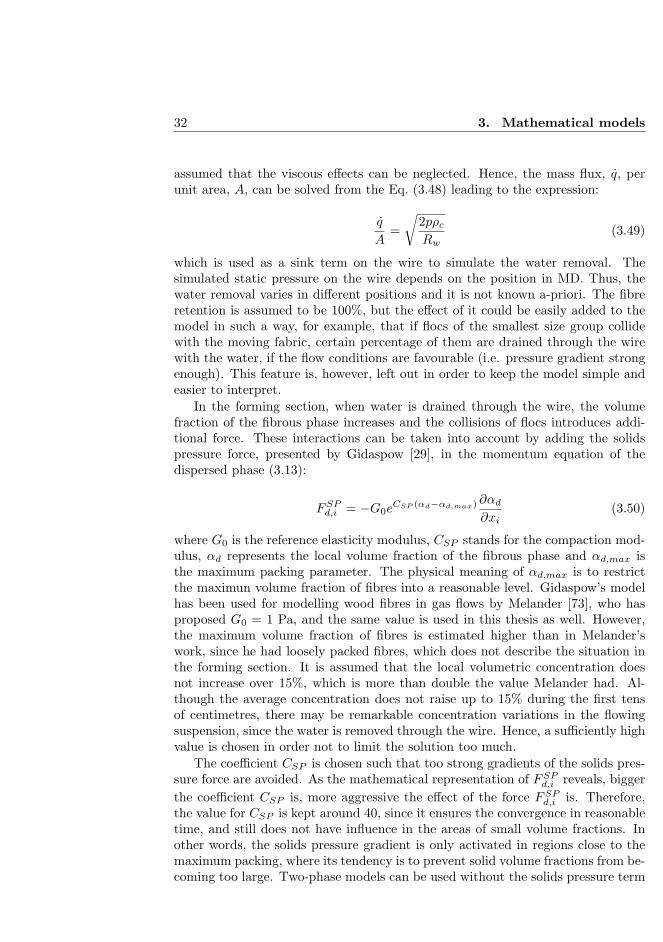
32 3. Mathematical models
assumed that the viscous effects can be neglected. Hence, the mass flux, q, perunit area, A, can be solved from the Eq. (3.48) leading to the expression:
q
A=√
2pρcRw
(3.49)
which is used as a sink term on the wire to simulate the water removal. Thesimulated static pressure on the wire depends on the position in MD. Thus, thewater removal varies in different positions and it is not known a-priori. The fibreretention is assumed to be 100%, but the effect of it could be easily added to themodel in such a way, for example, that if flocs of the smallest size group collidewith the moving fabric, certain percentage of them are drained through the wirewith the water, if the flow conditions are favourable (i.e. pressure gradient strongenough). This feature is, however, left out in order to keep the model simple andeasier to interpret.
In the forming section, when water is drained through the wire, the volumefraction of the fibrous phase increases and the collisions of flocs introduces addi-tional force. These interactions can be taken into account by adding the solidspressure force, presented by Gidaspow [29], in the momentum equation of thedispersed phase (3.13):
FSPd,i = −G0eCSP (αd−αd,max) ∂αd
∂xi(3.50)
where G0 is the reference elasticity modulus, CSP stands for the compaction mod-ulus, αd represents the local volume fraction of the fibrous phase and αd,max isthe maximum packing parameter. The physical meaning of αd,max is to restrictthe maximun volume fraction of fibres into a reasonable level. Gidaspow’s modelhas been used for modelling wood fibres in gas flows by Melander [73], who hasproposed G0 = 1 Pa, and the same value is used in this thesis as well. However,the maximum volume fraction of fibres is estimated higher than in Melander’swork, since he had loosely packed fibres, which does not describe the situation inthe forming section. It is assumed that the local volumetric concentration doesnot increase over 15%, which is more than double the value Melander had. Al-though the average concentration does not raise up to 15% during the first tensof centimetres, there may be remarkable concentration variations in the flowingsuspension, since the water is removed through the wire. Hence, a sufficiently highvalue is chosen in order not to limit the solution too much.
The coefficient CSP is chosen such that too strong gradients of the solids pres-sure force are avoided. As the mathematical representation of FSPd,i reveals, biggerthe coefficient CSP is, more aggressive the effect of the force FSPd,i is. Therefore,the value for CSP is kept around 40, since it ensures the convergence in reasonabletime, and still does not have influence in the areas of small volume fractions. Inother words, the solids pressure gradient is only activated in regions close to themaximum packing, where its tendency is to prevent solid volume fractions from be-coming too large. Two-phase models can be used without the solids pressure term

3.6 Modelling of dewatering 33
inside the headbox, for example, since the suspension is relatively homogeneousand dilute. However, neglecting the solids pressure force in the forming sectionwould lead to unrealistic concentration levels, since flocs would pack extremelytightly onto the wire surface.

Chapter 4
Model setup
The simulations presented in this thesis are all done by the commercial CFDsoftware ANSYS CFX. The implementation of each model, as well as model pa-rameters and boundary conditions used, are explained in the following sections.Even though modelling of some special characteristics, such as FOPD, is moredifficult with a commercial than with an in-house code in terms of convergenceand boundary conditions, the same approach is applied for all the characteris-tics in order to create an approachable basis for simulating the forming of thepaper structure. Certainly, choosing the modelling tool is always a compromise:with a commercial software, it is easy to program simple add-ons, but the wholecomplexity of the phenomena might not be implementable. On the other hand,if the simulation would be built on an in-house code the implementing of turbu-lence models, for example, would be a challenge itself. In addition, creating anin-house code including all the features presented below, would be extremely longwork. Therefore, it is reasonable to start the development of totally new model,such as the FFE, with a commercial tool, since it offers many sub-models alreadyimplemented, but still enables the modification of model parameters or even thereplacement of the sub-models with the own ones.
4.1 Model setup for the FOPD model
As stated earlier, the fibre orientation is studied in the headbox slice channel andin the jet. The situation can be assumed two-dimensional, if the effect of the slicechannel edges and secondary flow disturbances can be neglected. Thus, the flowproblem can be modelled with a 2D model consisting only of a vertical (x,y)-crosssection, i.e, papermaker’s (MD,z)-plane. However, including the FOPD model intoa standard 2D CFD simulation increases dimensions of the model up to three. Tobe able to handle this in a commercial software, the model is made geometricallythree dimensional such that the third coordinate axis stands for the angle φ belong-ing to [−π/2, π/2], see Fig. 4.1, and it is discretised in elements such as the otherdirections. Since the FOPD is implemented in the software as a passive scalar,
34
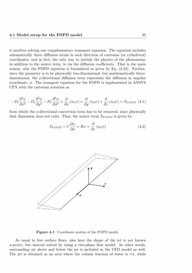
4.1 Model setup for the FOPD model 35
it involves solving one complementary transport equation. The equation includesautomatically three diffusion terms in each direction of cartesian (or cylindrical)coordinates, and in fact, the only way to include the physics of the phenomena,in addition to the source term, is via the diffusion coefficients. That is the mainreason, why the FOPD equation is formulated as given by Eq. (3.10). Further,since the geometry is to be physically two-dimensional, but mathematically three-dimensional, the z-directional diffusion term represents the diffusion in angularcoordinate, φ. The transport equation for the FOPD is implemented in ANSYSCFX with the cartesian notation as
−Dt∂2ψ
∂x2−Dt
∂2ψ
∂y2−Dr
∂2ψ
∂φ2+
∂
∂x(u1ψ) +
∂
∂y(u2ψ) +
∂
∂z(u3ψ) = SFOPD (4.1)
from which the z-directional convection term has to be removed, since physicallythat dimension does not exist. Thus, the source term SFOPD is given by:
SFOPD = C∂ψ
∂φ+Rψ +
∂
∂z(u3ψ) (4.2)
Figure 4.1: Coordinate system of the FOPD model.
As usual in free surface flows, also here the shape of the jet is not knowna-priori, but instead solved by using a two-phase flow model. In other words,surrounding air above and below the jet is included in the CFD model as well.The jet is obtained as an area where the volume fraction of water is ≈1, while

36 4. Model setup
in the surrounding air the volume fraction of water is ≈0. The jet can be solvedindependently from the FOPD model as the orientation does not affect the shapeof the jet. In this study the slice channel has been modelled as symmetrical andwithout slice bar. It contracts from 100 mm to 8 mm and has the length of500 mm. Numerical tests have attested that bigger the angle of the slice bar is,the more sensitive the geometry is for the convergence problems. This characteris emphasised when using the geometrically two-dimensional form of the FOPD.With a 1D approach and using the streamline approach it is possible to modellarger slice lip angles, but the simulations are not able to provide all the phenomenaoccuring at the slice opening. Thus, the mathematically two-dimensional form ofthe FOPD is used in this thesis.
The diffusion coefficients are estimated based on turbulent kinetic energy andon its dissipation rate, see [84]. Hyensjo has recently investigated deeply thedetermination of the rotational diffusion coefficient and presented three differenthypotheses based on turbulence theories [48]. He also suggested some optimisedvalues for parameters in the hypotheses. However, in this thesis, constant values,Dt = 0.0001 m2/s and Dr = 40 m2/s were used, since the anisotropic diffusion isa beta-feature of ANSYS CFX and the equations could not be implemented. Themagnitude of the z-directional coefficient (corresponding the rotational diffusion)was found by comparing the results given in [51]. The value of the rotationaldiffusion coefficient is an active area of research, and in an on-going project, muchmore bigger values have been proposed by Niskanen et al. [78]. They based theirsuggestion on the experiments performed for flexible fibres in the slice channelwith vanes. Those results differ remarkably from the ones presented by Ullmar[112], and the reason might be that Ullmar used flexible fibres in his experimentsto create the pulp suspension-like conditions, but observed rigid tracer fibres. Asa consequence, the results are not validated with experiments, but their reliabilityis assured by comparing them to previously reported studies, such as [51] and [85].
The FOPD model requires the boundary conditions like any typical CFD sim-ulation. The fibre orientation distribution is assumed to be isotropic at the inlet.In fact, if the turbulence generator pipes had been included in the model as it isdone in [78], there would be a profile with very small deviations from the isotropicdistribution. Therefore, in practice, the profile is neglible, since the most domi-nating effect is the channel acceleration. The inlet velocity is assumed constant,which means that the effect of the turbulence generator pipes is not taken intoaccount in the flow field simulation either.
At the edges, that is, φ = −π/2 and φ = π/2, periodic boundary conditionsare applied. Boundary conditions on the bottom and top walls as well as on thesurfaces of the jet are not trivial. In fact, the basic theory, how to implementthe wall boundary conditions in the FOPD model, is missing, although some goodexperimental work on the boundary layer behaviour of the fibre orientation hasbeen done [12]. The research is, however, rather fundamental, and according toits author, is not directly applicable in papermaking applications. Therefore, var-ious boundary condition types were compared to get confidence that the chosenone does not disturb the solution. The zero-flux boundary condition, ∇ψ · n = 0,

4.2 Model setup for the FFE model 37
where n is the normal of the wall, led to a nonrealistic solution, whereas theDirichlet-type boundary conditions gave reasonable solutions. That is, the proba-bility distribution was approximated using the analytic solution given in [85] andthe mean orientation angle was set to a wall direction on the walls. An analogousapproach was utilized for the jet as well.
The model provided similar results in the near-wall region as reported in theearlier study by Hyensjo [51], who avoided the determination of boundary condi-tions by choosing a model approach in which the FOPD is calculated postprocessedalong streamlines and out of the CFD software. His approach, as well the one pre-sented in this thesis, indicate that the head of the fibres tend to turn away from thewall. This proves that the chosen boundary condition does not disturb the solutiondue to a very small translational diffusion coefficient. This is also demonstratedwithin the results in Section 5.1, Figs. 5.4 and 5.7, for example.
4.2 Model setup for the FFE model
Since fibre flocculation is known to be strongly dependent on pulp properties, thesimulations are performed for two different pulps; one consisting of pine fibres andthe other of birch fibres (see Table 4.1). The mass concentration is converted tovolume concentration used in multiphase flow equations by multiplying the valueby 2, which is a commonly used rule of thumb. It is noteworthy, that the crowdingfactors of pine and birch differ significantly: according to definitions of Kerekes andSchell [60], the birch pulp is clearly in regime of forced collisions, while the pinepulp might already be dominated by continuous contact, see Table 2.1 in Section2.2. Hence, the flocculation phenomena of these two pulps may obey differentmechanisms.
Table 4.1: Characteristic properties of pulps used in simulations and experi-
ments.
Pine BirchAverage fibre length [mm] 2.05 0.92Average fibre diameter [µm] 22 16.7Fibre coarseness [mg/m] 0.206 0.114Mass concentration [%] 1 1Crowding factor [ ] 116 40
Since the FFE model is totally novel approach in flocculation modelling, themodel parameters need adjustment and validation. The results are validated withexperimental studies carried out for a sudden expansion of a circular pipe, similarto the pipes in the headbox turbulence generator. The experiments are not partof this thesis, but performed earlier by Salmela and Kataja [97], and thus, themethods used are only briefly introduced in the following subsection.

38 4. Model setup
To keep the modelling approach simple enough, only three model parametersare adjusted during the model validation phase, while the others are kept con-stant throughout the simulations. Until there is a good reason to believe thatgreater complexity provides more accurate information, it seems pointless to con-sider more parameters. Therefore, three ”simpler” model parameters are chosen tobe adjusted: the break-up coefficient, the coalescence coefficient and the internalstrength of a floc. To give an insight of the model structure for future researchers,the parameters and variables of model equations are now briefly reviewed. It is em-phasised that herein a parameter is given by the user, while a variable is solved bythe CFD code. In other words, the parameters depend on the material properties,which have to be defined specifically for different flowing media, while variablesare determined locally based on particular equations, and they are functions ofsimulated floc size, turbulence etc..
In the break-up model, that is, in Eqs. (3.36)...(3.39) the model variables, i.e.Nm, αm, dm, εc, and fBV , are calculated based on the local flow conditions andthe flocculated state of the suspension. They represent the number density of eachfloc size group, fibrous phase volume fraction, diameter of the parent particles, thecontinuous phase turbulent kinetic energy dissipation and the breakage volumefraction, respectively. The computation of the first four mentioned is straight-forward, and the last one, fBV , is based on the local kinetic energy of turbulenteddies (for more detailed explanation, see [70]). Hence, the only parameters to bedetermined for the break-up model are σ, which denotes the internal strength ofa floc, and CB , which is a supplemental break-up coefficient.
The variables in coalescence model, i.e. in Eqs. (3.40)...(3.47), are ηmn, tmn,ζmn, rmn, Amn and utm, which denote the collision efficiency, the time requiredfor coalescence, the actual contact time, the equivalent radius, the collision cross-sectional area and the turbulent eddy velocity of the length scale of the floc,respectively. The computation of these variables follow directly the equations pre-sented in Section 3.5.3. The model parameters the user has to determine are hinit,hcrit, CCT and σ, which denote the initial film thickness, the critical film thick-ness when rupture occurs, the turbulent coalescence coefficient and the internalstrength of a floc, respectively. One can, thus, notice that the internal strengthaffects both the break-up and the coalescence mechanisms. Determination of theturbulent coalescence coefficient is discussed together with the internal strengthof a floc and the break-up coefficient, since they are chosen to be the three modelparameters used for adjusting the model for fibre flocs. Moreover, since there areno better assumptions, the values for hinit and hcrit are set to be the default valuesproposed by the software, that is, 0.1 mm and 10−5 mm, respectively. The valuesmight be too small for flocs, since they are defined originally for bubbles, but acloser investigation is left for the future work.
The definition of the three chosen model parameters was quite a complex task,since their values are provided neither by experiments nor in the literature. Theroles of break-up and coalescence coefficients are quite obvious when looking atEqs. (3.36) and (3.45), since they appear only as dimensionless coefficients inthe model equations. The parameter describing the internal strength of a floc is

4.2 Model setup for the FFE model 39
analoguous to the surface tension, and hence, its adjustment for fibre suspensionflows requires special attention, since one can assume that it is dependent onpulp properties. Several authors, Kerekes and Schell [60] and Huber et al. [45],for example, have reported that flocculated state of the measured suspensionscorrelated somehow with their crowding factors. In addition, since flocs are smallcoherent networks possessing measurable strength (at least to some extent), muchof attention has been paid into the investigation of the yield stress of differentsuspensions.
Bennington et al. [8] performed extensive measurements for commercial woodfibre suspensions and synthetic fibre suspensions of low and medium consistency.They reported the yield stresses depending primarly on the local concentration ofthe suspension, but also fibre properties, such as aspect ratio and elastic modu-lus, was noticed to have an effect. The work was later extended by Dalpke andKerekes, who proposed simple power-law type of correlations [16]. However, themost fundamental work is performed by Farnood et al. who presented an analyticalequation describing the intra-floc forces [26] based on the model flocs. Farnood’smodel has the potential to model the internal strength of a floc, but since it is de-rived for a model floc having a form of ”X-star”, it unfortunately includes certainparameters that are not straightforwardly applicable to real flocs.
The numerical values for the three model parametres, namely, the break-upcoefficient, the coalescence coefficient and the internal strength of a floc, wereestimated by using a sensitivity analysis. In the gradient-based sensitivity analysisthe model parameters were searched making a comparison between simulated andexperimental average floc sizes (experiments were those performed by Salmela andKataja [97]). First, the initial values for the model parameters were chosen, and theFFE model was solved using these specified values. Next, one of the parameterswas varied a little, and the FFE model was solved again. This procedure wasrepeated for all the three parameters such that only one was modified at a time,while the others were kept constant.
An analysis was also required to formulate of a cost function to account for thegoodness of the performed modification. Hence, the cost function was formulatedsuch that it measured the difference between the simulated and measured averagefloc sizes at specified locations, and such that for a ”perfect match” the valueof the cost function would be zero. Next, the gradient of the cost function withrespect to three model parameters was calculated by using the finite differences ofthe simulated cost function values. Finally, by advancing in the negative gradientdirection with a chosen step length, better parameter values can be found. Theprocedure can be repeated until satisfactory model parameter values are found.
Since the saturation area is known to be very complex and at the same time im-portant when predicting the flocculated state of the suspension, the measurementpoints at that area were given more weight in the cost function. The weighting ofmeasurement points differently would, naturally, have provided slightly differentvalues for the model parameters. In addition, it must be emphasised that if the pa-rameters are strongly correlated, the gradient-based sensitivity analysis convergesslowly and would require tens of iterations of the method. It is worth noticing

40 4. Model setup
that one accurate CFD simulation of the FFE model in the turbulence generatorpipe requires approximately 6 CPU hours, and hence, for one sensitivity analysisstep, including three gradient component evaluations and at least two variationsof the step length, would require at least 5× 6 = 30 CPU hours.
Therefore, the algorithm was not repeated until the mathematically best pos-sible fitting was found, but the final tuning was done manually. It was possibleto see from the sensitivity analysis, that the break-up and coalescence coefficientssettled around 15 to 25 and 5 to 10, respectively, for both of the tested pulps, butthe internal strength of a floc depended on the pulp. The values giving the bestfitting compared to the experimental results were 20 for the break-up coefficientand 7 for the coalescence coefficient. The values for the internal strength of afloc were 4 N/m and 1.46 N/m for pine and birch pulps, respectively. In compar-ison with the studies of Farnood [26] and Wahren [113] who obtained values ofthe order of 10−10 Nm for the stored energy per floc, the proposed values soundhuge. In contrast, when comparing to results published by Bennington [8], Dalpke[16], Wikstrom [115] and their co-authors, the values 4 N/m and 1.46 N/m donot appear any unusual: for different pulps of 2 % mass concentration, they haveall obtained yield stress values ranging from 10 to 180 Pa. Hence, the order ofmagnitude for the floc strength parameter is justified. In addition, it was foundto fit with experimental data, as can be seen in the Section 5.2.2.
Once the parameters are adjusted in the turbulence generator pipe, the samevalues are applied also for other geometries for which no experimental data isavailable. Since the break-up and coalescence models take into account the accu-rately simulated local flow conditions and turbulence, it is assumed that there isno need for parameter tuning when studying different geometries. Naturally, dueto the lack of experimental material, this has not been proven within this thesis.However, if it turns out that the model parameters have to be readjusted everytime when the simulations are carried out for different geometries, then the wholebreak-up and coalescence model kernels should be revised. For further discussion,see Chapter 6.
Altogether, the flocculation is studied in three different geometries: in theturbulence generator pipe, in the slice channel and in the forming section. Thedetails of the simulated geometries, as well as boundary conditions applied, arebriefly introduced in Sections 4.2.2, 4.2.3 and 4.2.4.
4.2.1 On experimental reference material
The experiments used for validation of numerical results have been done earlier bySalmela and Kataja in the flow laboratory of VTT, and they are comprehensivelyreported in [97]. Part of the data set presented in this thesis is not fully included in[97], but has been considered in [38]. Hence, only a short description of methodsused are given here. It is to be emphasised that the author of this thesis hasnot participated in experiments, but only used them as a reference for the modelvalidation.
The flocculation has been measured downstream of a sudden backward facingstep in 16 positions, and in one position upstream of the step. The diameter of

4.2 Model setup for the FFE model 41
larger pipe was 26 mm and the diameter of the constriction 16 mm. The flow ratesrange between 0.5 l/s and 2.5 l/s.
The evolution of floc size has been measured optically using a back-light method.Typical image width was 30 mm and the height was the diameter of the pipe, i.e.26 mm. Thus, the measured floc size is determined for this specified volume and itis an average over the whole pipe. Since the pipe is circular, vertically transmittedlight integrates over smaller distance near the pipe walls than in the centre. Thus,the method may distort the data systematically depending on the radial position.Furthermore, the method cannot distinguish small overlapping flocs, but producesone large floc instead. However, the current experimental data is valuable formodel validation as it can be assumed to be accurate enough, at least qualita-tively, for the average floc size development in the axial direction. In addition,any other data including the floc size evolution was not available.
With regard to model validation, the data from simulations is taken in the samemanner as in the experiments, i.e. averaging the floc size over 16 specified volumes.The FFE model would enable the investigation of the local floc size distribution,but unfortunately no data for such a comparison was available. Thus, in futurework, this is an important issue to concentrate in.
4.2.2 FFE model in the turbulence generator
The turbulence generator pipe is modelled axisymmetrically in order to save thecomputational resources for accurate simulation of flocculation evolution. In ad-dition, only the circular part of the pipe was considered, since the purpose in thissimulation was to perform the model validation and adjust the required modelparameters. Since the floc size distribution data was available only from 20 mmupstream of the expansion, the simulation is carried out in two steps; first, theflow and turbulence were solved in simple pipe having the same diameter as thefirst pipe in order to obtain appropriate inflow conditions. This was an obligatorystep, because turbulence and velocity profiles had not been measured by Salmelaand Kataja [97]. Second, the acquired profiles were given as an input to the actualmodel, as well as the floc size distribution provided by the experiments. The ac-tual model consists of the 20 mm long constriction pipe and of the 1600 mm longexpansion section, see Fig. 4.2.
Figure 4.2: Axisymmetrical representation for the turbulence generator pipe
used in model validation.

42 4. Model setup
The effect of the number of size goups has been tested by performing thesimulations with 5, 10 and 20 size groups. It was noticed that 10 and 20 sizegroups gave almost similar results everywhere, but 5 size groups was not enoughto correctly predict the saturation area, see Fig. 4.3, and hence, 10 size groups wasdecided to use for all the simulations.
Figure 4.3: Comparison of the simulated dimensionless average floc volumes
given by different number of size groups (5, 10 and 20) to the experimental results
(experiments performed by Salmela and Kataja [97]).
4.2.3 FFE model in the slice channel
When the flocculation is studied in the slice channel, 60 mm wide model in thecross machine direction is used. The whole turbulence generator has not beenmodelled, but its effect on the CD-variation of the slice channel flow has been takeninto account by modelling six inlets to the slice channel, see Fig. 4.4. The velocityprofile of these inlets is assumed blunt, since it develops quite fast when enteringin the channel. The floc size distribution is set based on the experience, but aswill be demonstrated in Section 5.2.3, the FFE model posesses a ”self-balancing”character, and hence, the minor deviances in the inlet boundary condition do notcontort the solution. The slice channel is 600 mm long and includes two wedges(stiff, contracting lamellas), which end 120 mm before the slice opening.
The reliability of the carrying phase modelling has been assured (reported in[34]) by comparing the 3D simulations for the slice channel with the tailored slicechannel model HOCS Fibre [36], which, in turn, has been validated with the pilotmachine measurements in [35]. Both the MD velocity and pressure were measuredby using a pitot tube along several CD lines inside the slice channel. It is alsoshown in [34], that both the HOCS Fibre and the 3D model used in this thesis,predict the CD velocities accurately enough. Hence, it can be assumed, that flowfield simulations are accurate enough in order to give a reliable basis for the FFE

4.2 Model setup for the FFE model 43
Figure 4.4: Slice channel with wedges.
modelling.
4.2.4 FFE model in the forming section
For the modelling of flocculation in the forming section, a 2D approach is used,since the system of equations for a three-phase flow including 10 conservation equa-tions for different size groups would be extremely time consuming and challengingto solve in 3D. The forming is studied in the Fourdrinier-type of forming sectionincluding the free jet and the preceding slice channel with two wedges and theslice bar, see Fig. 4.5 for the overall view, and Fig. 4.6 for the detailed view. Thefabric remains straight in the impingement area, i.e. the wire tension is assumedinfinite. In other words, the wire is modelled as a flat moving wall the position ofwhich is assumed known. In order to study the initial dewatering area, only thefirst 40 cm of the wire is included in the model.
The shape of the free jet, as well as the impingement of the jet, is not knowna-priori, but they are solved with the free surface model. The flow is, therefore,modelled as a turbulent three-phase flow, including water, fibrous phase and thesurrounding air. This approach reveals the natural physics of the phenomena,since any assumptions of the jet contraction after the slice opening or jet expansionafter the impingement are not made. In several studies, [6] and [56], for example,the jet expansion has been neglected. Dalpke et al. [17] took the jet expansioninto account, but in their simulation the flow was laminar and there were noconcentration changes, since the suspension was modelled as pure water.
In the beginning of the slice channel the flow is assumed to have constantvelocity and the floc size distribution has been set based on experience such asfor the 3D slice channel. Outside the headbox, for the upper part of the airflow, the inlet boundary condition is set at constant velocity, and for the airinlet below the free jet, an opening condition with pressure level is used. Thisboundary condition lets the fluid flow in or out, and has, therefore, less effects to

44 4. Model setup
Figure 4.5: Geometry for the forming section simulation
Figure 4.6: Detailed view of the slice opening area of the geometry for the
forming section simulation
the overall flow conditions than other boundary condition types. This is the mostconvenient boundary condition type for the air below the jet, since it imitatesthe real conditions in the papermachine forming section. At the outlet of thedomain there is naturally a pressure boundary condition, and the upper part ofthe surrounding air is restricted with a free slip wall.
The modelling of the moving wire requires special attention. The mass con-centration of the suspension leaving the headbox is 1%, and during the dewateringthe concentration increase is taken into account. The water removal and the solidspressure force have been programmed as add-ons in the commercial CFD code.The solids pressure force is present in all the domain, but it is activated only inareas where fibrous phase concentration approaches the maximum package, thatis, in the water removal area. Further, in addition to the water removal, the mov-ing wire must also be able to let the air pass through. This is accomplished bysetting a similar sink term for air than for water, but naturally modifying the wireresistance such that a balanced solution is obtained.

4.2 Model setup for the FFE model 45
The effect of the forming section on the floc size evolution is studied for threejet-to-wire ratios (J/W): J/W=0.9, J/W=1.0 and J/W=1.1, in order to demon-strate the effect of the shear on the development of the local floc size. The jet speedhas been kept same for all the different simulations, 24 m/s, and the wire speed hasbeen varied. The chosen jet-to-wire ratios give the wire velocity of ≈21.8 m/s forthe drag mode (i.e. J/W=0.9) and ≈26.7 m/s for the rush mode (i.e. J/W=1.1).The computations are performed only for one web resistance, since the purpose ofthis work was not to study the dewatering phenomena in detail. In addition, thenumber of floc size groups is restricted to 10 also in this application, for keepingthe needed computational resources reasonable.

Chapter 5
Numerical results and model validation
5.1 Fibre orientation in the slice channel and in the jet
5.1.1 On the representation of the FOPD results
When examining the numerical results, it is worth to keep in mind that the modelis constructed in a way that the x-axis follows the centreline of the slice channelin MD. The position x = 0 lies at the slice opening, so the negative values of xsituate inside the slice channel. The papermaker’s z-direction is described withthe vertical y-axis the origin being at the centreline (see Fig. 4.1).
Figure 5.1: Visualisation of the orientation distribution 3 mm above the centre
line throughout the slice channel and the jet.
46

5.1 Fibre orientation in the slice channel and in the jet 47
The numerically solved FOPD model provides the whole probability distribu-tion field. One example of a 2D field is presented in Fig. 5.1, which illustrates theorientation distribution 3 mm above the centre line throughout the slice channeland the jet. This kind of representation is not, nevertheless, very easy to inter-pret when printed out on a paper, and thus, the distributions are presented withcustomary graphs for different locations.
5.1.2 Development of fibre orientation in the slice channel and in thejet
At the beginning of the slice channel, x = −500 mm, the fibres are supposed to beisotropically oriented. Then, the acceleration of the flow starts to orient fibres inthe main flow direction, which can be seen in Fig. 5.2, where the first three curvesrepresent the situation inside the slice channel at the centreline. The fibres aremost strongly oriented at the slice opening, x = 0 mm, but, in the jet (x = 10 mm,x = 30 mm, x = 150 mm), the orientation tends to randomize due to the absenceof acceleration and shear forces. The results at the slice channel centreline agreewell with the previous study reported in [85].
The change in the maximum probability peak along the centreline when the jetenters into free air can be seen even more clearly in Fig. 5.3. The peak decreasessignificantly during the first few centimetres, after which the role of convectionin carrying the fibre orientation profile downstream in the jet can be seen. Tothe author’s knowledge, the FOPD model has not been applied to the contractingjet before. Hyensjo had an extension after the slice channel imitating the jet,but it was not contracting [48]. Nevertheless, according to test performed withthe same 1D solver that was used by Olson et al. [85], a 1D model presumes tooslow dampening of the maximum value in the jet. This proves the importanceof utilising the mathematically two-dimensional form of the FOPD model whendesiring accurate results in the presence of strong velocity gradients.
To examine more closely what happens inside the slice channel, the fibre orien-tation distributions are illustrated at various vertical positions 150 mm upstreamof the slice opening in Fig. 5.4. In the figure, the y-coordinate varies between -15mm and 15 mm (y-15 and y15 in the graph) when the whole channel depth is fromy = −18 mm to y = 18 mm, and y0 is in the middle. The orienting effect of thebottom and top walls can be seen clearly in Fig. 5.4. The peak is higher and thedeviation narrower near the walls, that is, the fibres are more strongly orientedin the flow direction. Also, the fibres are not oriented in the paper plane direc-tion (except at the centreline), but are shifted slightly due to the presence of thewalls, which can be seen in the displacement of the distribution peak from zero.It is also noteworthy that the fibres in the region near the wall are inclined morethan is the angle of the wall. This phenomenon has been reported already in theearlier study [49]. Since the geometry modelled and all boundary conditions aresymmetrical, the numerical results are symmetrical too, as in Fig. 5.4. Thereforein the following figures, only the upper half of the slice channel is presented.
The jet contraction immediately after the slice opening affects the fibre orien-tation distribution strongly, as can be noticed in Fig. 5.5. (It is worth of noticing

48 5. Numerical results and model validation
Figure 5.2: Development of the fibre orientation distribution along the centreline
of the headbox slice channel and of the jet.
Figure 5.3: Development of the maximum value of the fibre orientation distri-
bution along the centreline of the headbox slice channel and of the jet.
that the abscissa of the graph is different from the previous illustrations in orderto be able to better examine the details.) As soon as the flow enters into free air,there are no solid walls restricting the flow direction, and the effects of frictionand acceleration cease suddenly. The fibre orientation in the middle of the slice

5.1 Fibre orientation in the slice channel and in the jet 49
Figure 5.4: Fibre orientation distribution at various vertical positions inside the
slice channel, 150 mm upstream of the slice opening.
Figure 5.5: Fibre orientation distribution at various vertical positions at the
slice opening.
opening is the customary Gaussian-like curve, but already 2.5 mm above the cen-treline there appears a secondary peak. When approaching the wall, the secondarypeak increases while the main peak decreases such that, just near the wall, thesecondary peak is notably higher than the main one. The main peak is due to

50 5. Numerical results and model validation
Figure 5.6: Fibre orientation distribution at various vertical positions 5 mm
downstream of the slice opening.
Figure 5.7: Fibre orientation distribution at various vertical positions in the
headbox jet, 50 mm downstream of the slice opening.
the presence of the wall, such as inside the channel, whereas the secondary peakcan be explained by the sudden contraction of the jet: the velocity gradients atthe slice opening are steeper and therefore they orient the fibres more towards thecentre of the jet than would be the effect of the wall only. Hence, at a narrow

5.2 Fibre flocculation inside the headbox 51
area close to the slice lip, there are two almost equally probable orientation angles.This is the first demonstration of this kind of extraordinary phenomenon basedon numerical simulations. The effect does not procede far in the jet; as a matterof fact, only 5 mm after of the slice opening it can barely be distinguished, as canbe noticed in Fig. 5.6, and 10 mm downstream of the slice opening it has alreadyfaded out.
As stated before, fibre orientation tends to randomize in the slice jet. Theorientation distribution changes rapidly from the strongly oriented towards themore random one during the first few centimetres. After that, it develops moreslowly (shown in Fig. 5.3). To study the vertical variation of the fibre orientationdistribution inside the jet, the distributions are illustrated in Fig. 5.7 at the po-sition x = 50 mm downstream of the slice opening at the centreline (y0), 1 mm,2 mm and 3 mm above it. It can be seen that fibres are more randomly orientedat the centreline than near the jet surfaces, so the effect of the slice channel wallsand especially of the jet contraction is visible further in the jet, too.
5.2 Fibre flocculation inside the headbox
5.2.1 On the representation of the FFE results
The experimental data by Salmela and Kataja [97] used for the validation ofthe FFE model is presented with certain procedure, and therefore, it is wise togo through the methods before looking deeper to the results. Already in earlierstudies of flocculation phenomena, Karema et al. [57] have mostly presented theirresults using the dimensionless floc volume:
V ∗f =< Lx >< Ly >
2
l3f(5.1)
where lf is the length-weighted mean fibre length, Lx and Ly are the length-weighted mean floc dimensions in flow direction and cross direction, respectively,and <> denotes average over the image area and over the 200 exposures taken ateach imaging position. Using the dimensionless floc volume is justified in certainoccasions, since it facilitates the comparison of different pulps within a same graph,but on the other hand, this procedure conceals the physical phenomenon, becauseone cannot straightforwardly see the real floc sizes. As can be noticed in Fig. 5.8,for different pulps the same dimensionless volume (top) may signify remarkablydifferent real floc volumes (bottom).
In addition, Karema et al. have presented the evolution of floc size as a func-tion of mean residence time instead of the axial distance. This is a very suitablemethod, because it facilitates the comparison between different flow rates andenables the determination of accepted residence time, when designing a new tur-bulence generator, for example. The time t = 0 is set at the beginning of thesudden expansion and the spatial position is converted in temporal position usingsimply the mean flow velocity. However, when investigating a specified process in

52 5. Numerical results and model validation
Figure 5.8: Comparison between the dimensionless (top) and real floc size (bot-
tom) for two simulated data sets.
the wet end, it is also very informative to plot the data with the real dimensions,as done below for the results of slice channel and forming section.
Further, it has been a common procedure to illustrate the results using a log-arithmic scale for both the abscissa and the ordinate. This might be quite mis-leading, as can be noticed when comparing Fig. 5.9 (top) to the Fig. 5.8 (bottom).A logarithmic scale may be useful in examining the gereral trends, as shown innext subsection, but when validating the CFD model, it accentuates too muchthe differencies within the small size groups and fades out the variations in biggersize groups. Further, when plotting the same situation using the floc diameteras an ordinate, one gets an illustration which is perhaps easier to connect to theflocculated state of the suspension or even to the resulting formation, see Fig.5.9 (bottom). On the other hand, Fig. 5.9 (top) may be useful when turning theattention to the resulting local basis weight.

5.2 Fibre flocculation inside the headbox 53
Figure 5.9: Comparison between the floc volume (top) and floc diameter (bot-
tom) for two simulated data sets.
5.2.2 Model validation - flocculation in the turbulence generator pipe
Salmela and Kataja permormed a comprehensive set of experiments for the tur-bulence generator pipes [97], and their measurements are used for the model val-idation. The model parameters have assumed to depend on the flowing medium,but not on the geometry or flow rate, since the break-up and coalescence modelsalready include the physics of the flow. Once the parameters have been deter-mined in the turbulence generator pipe, the FFE model is used to investigatewhat happens to the floc size in the different parts of the headbox and in theforming section.
The model validation was carried out for three different flow rates: 1.5 l/s, 2.0l/s and 2.5 l/s, and for two different pulps, pine and birch, presented in Table 4.1in Section 4.2. The simulated flow rates correspond the average flow speeds of 2.8m/s, 3.8 m/s and 4.7 m/s, respectively, in the turbulence generator pipe.

54 5. Numerical results and model validation
Figure 5.10: Measured (top) and simulated (bottom) floc size evolution of pine
pulp as a function of the mean residence time for the flow rates of 1.5 l/s, 2.0 l/s
and 2.5 l/s (experiments performed by Salmela and Kataja [97]).
In order to examine the general trends of the floc size evolution, it is usefulto compare Fig. 5.10 (top) and (bottom), where the floc size evolution of pinepulp has been illustrated for the whole set of different flow rates for experimentaland simulated results, respectively. Similar investigation is performed for birchpulp in Fig. 5.11. For the trend comparison, the logarithmic scale is useful. Thesimulated curves representing different flow rates overlap on the regrowth area,the minimum floc size being dependent on the flow rate. This is consistent withthe experiments. Further, when reaching the saturation area, the simulated curvesseparate in a similar way as the measured ones, and hence, the general trends arewell captured. In contrast, the minimum floc size appears to differ more than

5.2 Fibre flocculation inside the headbox 55
Figure 5.11: Measured (top) and simulated (bottom) floc size evolution of birch
pulp as a function of the mean residence time for the flow rates of 1.5 l/s, 2.0 l/s
and 2.5 l/s (experiments performed by Salmela and Kataja [97]).
other areas. The model seems too insensitive to predict correctly the effect ofthe increased turbulence and shear stress just after the expansion: the modelledcurves differ only slightly from each other, while there are larger differences inthe experimental ones. However, it has to be kept in mind that the logarithmicrepresentation accentuates the differencies in small floc volumes, and as can beseen below in Figs. 5.12 and 5.13, the model predictions are not that inaccurateat all.
Next, it is worth to take a closer look and compare the simulated pine pulp re-sults to experimental ones flow rate by flow rate; see Fig. 5.12, where ”Exp.” refersto experimental data and ”CFD” to simulations. It can be noticed that the shapes

56 5. Numerical results and model validation
Figure 5.12: Simulated and measured floc size evolution of pine pulp as a func-
tion of the mean residence time for the flow rate of 1.5 l/s.(top), 2.0 l/s (middle)
and 2.5 l/s (bottom) (experiments by Salmela and Kataja [97]).

5.2 Fibre flocculation inside the headbox 57
Figure 5.13: Simulated and measured floc size evolution of birch pulp as a
function of the mean residence time for the flow rate of 1.5 l/s.(top), 2.0 l/s
(middle) and 2.5 l/s (bottom) (experiments by Salmela and Kataja [97]).

58 5. Numerical results and model validation
of the simulated curves are similar to the experimental ones, which means that thegeneral behaviour of both the floc break-up and the coalescence phenomena arewell captured. The model slightly underestimates the minimum floc size occurringimmediately after the sudden expansion, especially for the lowest flow rate. Incontrast, the further growth of flocs is well predicted, the deviation between thesimulated and experimental results being only about 10 % for the two highest flowrates. This result is of great value; this is the first occasion where fibre floccula-tion has been predicted quantitatively (and even with the acceptable accuracy),while previous researches have provided only some approximative information ofthe flocculation phenomenon, such as flocculation index or flocculation tendency.The new model has also demonstrated its suitability for the saturation area, whichis known to be very complex. In fact, the percentual errors at the named areaare smaller than in any other location, less than 10 % for two highest flow rates.Given that the saturation phenomenon is the most difficult from the modellingpoint of view, the results can be considered quite impressive.
As mentioned earlier in Section 4.2, the internal floc strength for the birchpulp was found to be 1.46 N/m, while the value for pine was 4 N/m. Hence, therelation between the internal floc strengths of the pine and the birch pulps is ∼2.7. This was found to be exactly the same as the relation between the crowdingfactors of the two named pulps:
Nmf,pineNmf,birch
=σpineσbirch
(5.2)
where Nmf stands for the crowding factor and σ for the internal strength. Tothe author’s knowledge, this is the first demonstration of this kind of dependencybetween floc strength and crowding factor. The finding is supported by the resultsof Huber et al. [45]; they reported the effect of the crowding factor and flowspeed on the flocculation index, and proposed a simple correlation model basedon experimental data. Also Kerekes and Schell [60] have reported that flocculatedstate of the measured suspensions correlated somehow with their crowding factors,as already mentioned.
As can be seen in Fig. 5.13, the beginning of the regrowth area is not as wellpredicted for birch as it is for pine. The slope of the simulated curve is steeper,and the simulations also predict that coalescence occurs later than in measure-ments. However, at the end of the regrowth, as well as in the saturation area, theagreement between simulations and experiments is very good. The reason, whythe simulations of the birch pulp in the regrowth area do not agree with measure-ments as well as pine, might be that the mentioned pulps are in different regimes.Consequently, their flocculation may occur differently, and the model parametersshould be adjusted in order to take this behaviour into account. However, theFFE model works acceptably for both of the pulps used in the simulations, andhence, the presented parameter values are used for all the other geometries.

5.2 Fibre flocculation inside the headbox 59
5.2.3 Flocculation in the turbulence generator
The available experimental data provides information only about the evolution ofthe dimensionless mean floc size, but with CFD simulations many other intrestingaspects can be studied. Although all the presented phenomena might not be abso-lutely correctly predicted, they give, nevertheless, relevant information of the localphenomena and can be used to determine, wheather the simulation is reliable ornot. Therefore, some intresting findings are presented and discussed below. Wheninvestigating the countour plots, it is worth to keep in mind that the simulationsare performed axisymmetrically, and hence, only the half of the pipe is presented.
The evolution of the different size groups can be examined by representing thesize fractions as a function of the residence time, see Fig. 5.14. The data is takenin the same manner as for the model validation and for the experiment, that is,averaging over a volume covering the whole pipe diameter and having the lengthof 30 mm in the flow direction. It can be observed that immediately after theexpansion, the number of the smallest flocs (group 1) is very high and there arepractically no large flocs. However, the coalescence process starts to dominate veryshortly, and hence, the number of the smallest flocs drops dramatically, while theamount of the medium size flocs starts to increase. The size fraction of the biggestflocs begins to grow later. This indicates that the coalescence phenomenon occurssequentially; first, small flocs agglomerate together to form medium size flocs,which, in turn, coalesce into larger flocs.
Figure 5.14: Simulated evolution of the different size groups of the pine pulp as
a function of the mean residence time for the flow rate of 2.0 l/s.
The Fig. 5.14 reveals that there is a remarkable difference in the volume frac-tions of two smallest size groups in the beginning of the expansion, and the similareffect can be seen at the end of the pipe between two largest size groups. Thisindicates that higher number of size groups would be needed to more accuratelypredict the size group distribution. However, as seen in Fig. 4.3 in Section 4.2,

60 5. Numerical results and model validation
the increase of size groups did not affect the mean floc size. As a consequence, thechosen number of size groups is justified, until more accurate experimental dataon different floc sizes for the model validation is available.
Since the FFE is a real two-fluid model, one can also examine such phenomenaand flow characteristics which would remain completely unknown with one-phaseapproach. Fig. 5.16 illustrates the variations in the local concentration of thefibrous phase right after the expansion. It can be noticed that the FFE correctlypredicts that there are practically no fibres in the backflow eddy. In addition, themean floc diameter, for example, can be studied elaborately in different positions.The local mean floc size right after the sudden expansion is presented in Fig. 5.17.The flocs are clearly smaller near the pipe wall region than in the middle. Thisis caused by turbulence, which occurs due to the expansion, as can be seen inFig. 5.18. The floc size decreases quickly right after the sudden expansion as thebreak-up forces dominate. It is worth to keep in mind that in the area presentedin Figs. 5.16...5.18 the reflocculation has not been started yet.
One interesting finding is also the ”self-balancing” effect of the FFE model.A pipe geometry with different contraction diameter was modelled, and since anyexperimental data for fibre floc size distribution at the inlet was not available, twodifferent distributions were tested. One distribution was chosen to represent thesituation where there would be plenty of small flocs and the other distribution wasweighted for the medium-sized flocs. The distributions are given in Table 5.1. Ascan be seen in Fig. 5.15, the mean floc size curves differ only in the very beginningof the pipe expansion. This means that the mechanisms of the phenomena ”takecare” that the floc size evolution is strongly controlled by the local flow field andturbulence. Therefore, it enables the simulation of such geometries for which theexperimental data does not exist, since even though the initial guess for the inletboundary condition would be somewhat wrong, the model still predicts correctlythe floc size evolution.
Figure 5.15: Selfbalancing character of FFE model.

5.2 Fibre flocculation inside the headbox 61
Figure 5.16: Simulated volume fraction of fibrous phase after the sudden pipe
expansion. The height of the step is 5 mm.
Figure 5.17: Simulated mean floc diameter after the sudden pipe expansion.
Figure 5.18: Simulated turbulent kinetic energy after the sudden pipe expan-
sion.

62 5. Numerical results and model validation
Table 5.1: Volume fractions of two different fibre floc size distributions for the
self-balancing test.
Size group Small-size Medium-sizenumber weighted weighted
1 0.3 0.032 0.2 0.053 0.15 0.14 0.1 0.155 0.1 0.36 0.05 0.27 0.05 0.18 0.03 0.059 0.02 0.0210 0 0
5.2.4 Flocculation in the slice channel
The floc size evolution in the slice channel is an intresting subject to investigate,since in modern headboxes, the design of the slice channel has recieved a lotof attention. Unfortunately, no experimental data for comparison is available.Nevertheless, the fibre floc size seems to behave quite reasonably, as can be seenin Fig. 5.19, where the mean floc size is plotted along the line going through theslice channel in MD. (The line is situated in the middle of the two wedges inz-direction and in the middle of the outlet of turbulence generator pipe in CD-direction.) When entering into the slice channel, the mean floc diameter is about3 mm, but near the slice opening the small flocs have coalesced and formed biggerones. It is worth of pointing out that the graphs in Figs. 5.19 and 5.20 are notplotted till the end of the slice channel, since the examination of a single linewould provide misleading results: In Fig. 5.26 it can be noticed that floc sizeevolution follows streamlines, and hence, a straight line would present results theinterpretation of which would be somewhat difficult.
Investigation of evolution of the different size groups in Fig. 5.20 reveals thatcontrary to the situation in the turbulence generator pipe expansion in Fig. 5.14,ten size groups is sufficient to reliably predict the floc size distribution in the slicechannel, since the differencies in the volume fraction between two smallest andtwo largest size groups are relatively small. Flocs of all sizes start to coalesce rightafter the beginning of the slice channel, but the process remains quite calm, andthe overall floc size grows relatively slowly. This is due to flow velocity, which iskept quite high with the wedges, and naturally the shear induced by walls thatbreaks up the flocs. The simulated floc size development in the slice channel iscongruent with the ”real-life” findings. Also, the recent headbox development isfocusing in avoiding the re-flocculation by minimizing the suspension residence

5.2 Fibre flocculation inside the headbox 63
Figure 5.19: The evolution of the mean floc diameter inside the slice channel,
along the line at the middle of the turbulence generator pipe.
Figure 5.20: The evolution of different floc size groups inside the slice channel,
along the line at the middle of the turbulence generator pipe.
time from the turbulence generator to the forming zone, and also by using wegdesinstead of lamellae.
The overall development of the flocculated state of the suspension can be stud-ied with Figs. 5.21 and 5.22 where the local mean floc size and the local velocity,respectively, are presented at the centre plane between two wedges. The meanfloc size is not even in the cross machine direction, since there is velocity and tur-bulence profile due to the turbulence generator, which was modelled by 2x3 tubeentries. The effect of turbulence generator proceeds far downstream and remainsvisible at the slice opening as well. The floc size near the slice opening may by

64 5. Numerical results and model validation
Figure 5.21: The local mean floc diameter inside the slice channel at the centre
plane between two wedges.
Figure 5.22: The local velocity profile inside the slice channel at the centre
plane between two wedges.
slightly mispredicted due to the vicinity of the outlet boundary, but still it can beconcluded that strong velocity gradients and turbulence created by the slice lipreduce the mean floc size significantly at the end of the slice channel.
One extraordinary detail is the prediction that the floc size would remain sig-nificantly smaller in the middle of the figure, at the wake of turbulence generatorpipe walls. (Same effect occurs also at the top and bottom of the figure, wheresymmetric boundary conditions are applied, even though it is not very clearlyvisible.) This effect can be closer examined with the Fig. 5.23, which representsthe detailed view of the slice channel. (The black lines in Fig. 5.21 indicate thelocation of the detailed view.) Smaller mean floc size cannot directly be explainedby any single property of the flow field, but it must be somehow connected toturbulence and strong velocity gradients occuring in the wake. The turbulencekinetic energy is presented in Fig. 5.24 for the comparison.
It is also intresting to examine the mean floc size evolution between the wedges.It can be seen in Fig. 5.25 that floc size is smaller near the walls, which is naturally,caused by the shear layer near the wall. The distance between the wedges is not

5.2 Fibre flocculation inside the headbox 65
Figure 5.23: Detailed view of the local mean floc diameter inside the slice
channel at the centre plane of turbulence generator pipe.
Figure 5.24: Detailed view of the turbulent kinetic energy inside the slice chan-
nel at the centre plane of turbulence generator pipe.
exatly the same, which causes the differencies in the countour: the floc size is bigat larger area in the middle gap than in the top and the bottom gaps. Also theeffect of the slice bar is visible in the upstream, which can be concluded in theasymmetry of the contour of the middle gap, see Fig. 5.26. The end of the wedgesis 0.5 mm thick, and obviously, no deattachment of the flow occurs, since the meanfloc size profile remains stable.
As mentioned earlier in the Section 3.5, it is still a matter of debate, whichmechanism breaks up the flocs. Some researchers claim that it is the elongation,while the others say it is turbulence. In the slice channel there is a continuousacceleration of the flow, i.e. elongation, but as seen with the results presented
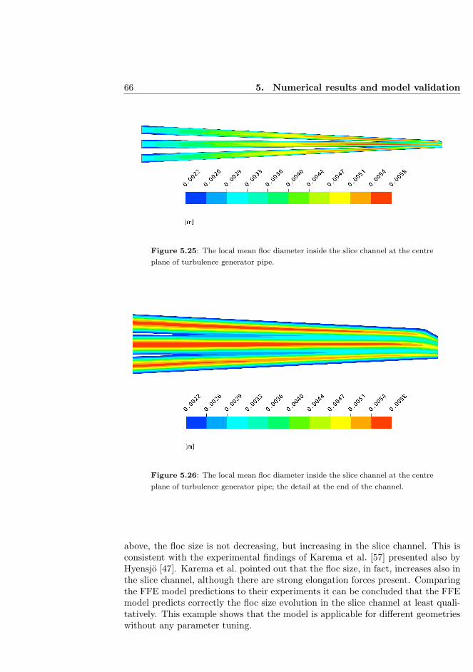
66 5. Numerical results and model validation
Figure 5.25: The local mean floc diameter inside the slice channel at the centre
plane of turbulence generator pipe.
Figure 5.26: The local mean floc diameter inside the slice channel at the centre
plane of turbulence generator pipe; the detail at the end of the channel.
above, the floc size is not decreasing, but increasing in the slice channel. This isconsistent with the experimental findings of Karema et al. [57] presented also byHyensjo [47]. Karema et al. pointed out that the floc size, in fact, increases also inthe slice channel, although there are strong elongation forces present. Comparingthe FFE model predictions to their experiments it can be concluded that the FFEmodel predicts correctly the floc size evolution in the slice channel at least quali-tatively. This example shows that the model is applicable for different geometrieswithout any parameter tuning.

5.3 Fibre flocculation in the forming section 67
5.3 Fibre flocculation in the forming section
Since there is no experimental data available for the validation of the floc sizeevolution in the forming section, it is worth to start to examine the results bylooking the flow field in detail in order to ensure that the simulation of the complexflow field is adequately performed. The complicated phenomena of the flow fielddetermine the flocculation process, and therefore, the reliability of the flow fieldmodelling is one of the key issues.
In Fig. 5.27 it can be seen, how the velocity profile of water develops down-stream of the wedges (far left in the illustration). The slice bar modifies the flowprofile by inducing a low velocity area at the top of the channel just before theend, and accelerates the upper part of the jet faster than the rest of the jet. It isalso worth of noticing that the velocity profile created by wedges is present in thejet after the vena-contracta, as well. The jet contraction coefficient predicted bysimulations is ≈0.83, which is very typical value for this kind of construction.
The most critical area from the modelling point of view is the jet impingementon the moving wire. At the location where the jet hits the wire, an abrupt decreasein flow speed occurs above the fabric, and the jet expansion can be noticed whenlooking carefully the upper surface of the jet. This gives rise to a momentary de-crease in the whole jet speed at this position, and it occurs for all jet-to-wire ratiosas will be shown below. However, very quickly the speed of the jet increases again,but the streaks in the velocity profile are not present any more. The developmentof the velocity profiles at the impingement area gives valuable information of theflow phenomena, and hence it is worth to look at them more closely.
The velocity profiles over the whole thickness of the jet are presented in Fig.5.28 for the J/W=1.0, and thus, both the jet and wire velocity were 24 m/s. Thejet hits the wire ≈27 mm after the bottom lip, where x = 0, and the first velocityprofile in the illustration (denoted with x30) is then right after the impingement.(The positions x30, x50, x70, x100, x150, x200, x250 and x300 in following illus-trations refer to distance from the bottom lip in millimeters.) The strong decreasein the flow speed presented in Fig. 5.27, can also be seen when looking at the curveof x30 in Fig. 5.28: at the wire surface the water flows naturally at the wire speed,but right above, it has remarkably lower velocity due to the impact caused bythe impingement. Also the overall speed is less than 24 m/s at the impingementzone, but the profile starts to develop quite quickly, as seen with curves x50 andx70, for example. When looking carefully the upper ends of the curves at differentpositions, it can also be noticed that the jet thickess is decreasing when suspensionis moving downstream in the forming section. This is, naturally, due to the waterremoval.
When comparing the velocity profiles for three different jet-to-wire ratios,J/W=0.9, J/W=1.0 and J/W=1.1, (Fig. 5.29) it can be noticed that the phe-nomena at the impingement area are very similar and independent of the speeddifference between the jet and the wire. For all the three simulations the flowvelocity right above the wire is ≈18 m/s, and thus, only the velocity gradient atthe impingement is higher, if the wire speed is higher. Also the profiles of tur-

68 5. Numerical results and model validation
Figure 5.27: The impingement of the jet for J/W=1.0. The color represents the
speed of the water.
Figure 5.28: Water velocity profiles above the wire surface at 8 different MD
positions for J/W=1.0. x30 denotes the MD location 30 mm downstream of the
bottom lip, etc.

5.3 Fibre flocculation in the forming section 69
bulent kinetic energy (Fig. 5.30) attest that the jet impingement dominates thesituation in the beginning, since the kinetic energy at x30 is very similar in allthe illustrations, and hence, independent on the jet-to-wire ratio. A closer lookinto the turbulent kinetic energy profiles reveals that they are very similar for theJ/W=1.0 and J/W=1.1, while J/W=0.9 differs from them significantly. Also, thevelocity profiles indicate that for the drag mode there is a remarkable shear abovethe moving wire from the beginning of the forming section, while for the rushmode the drag forces do not to become important until the position x150.
The two-fluid simulation enables the inspection of the flow field separately forboth of the phases. The Fig. 5.31 reveals that the velocity profiles of the flocphase are not as smooth as those of water, but the speed differences induced bythe wedges in the slice channel are still present in the forming section. In addition,the decrease of velocity is not as dramatical for flocs as it is for water: when theflow velocity right above the wire is ≈20 m/s for flocs, for water it was only ≈18m/s. Moreover, for the floc phase it takes longer to be accelerated again at thevelocity of the free jet: the overall velocity does not reach 24 m/s until x150 forJ/W=0.9 and J/W=1.0. These events are probably due to the bigger viscosity ofthe floc phase.
Since the purpose of this work is not to study the dewatering phenomena indetail, computations were performed only for one web resistance. Hence, the de-watering is similar for all three jet-to-wire ratios, since the water removal dependson pressure, which does not change, when the wire velocity is modified. As canbe seen in Fig. 5.32, the dewatering is very strong at the location, where the freejet impinges the moving wire, which is ≈27 mm downstream of the bottom lip(x = 0 at the end of the bottom lip). Downstream of this point the dewatering israther gentle, and it remains quite stable at the initial dewatering zone. The pres-sure field at the beginning of the forming section is illustrated in Fig. 5.34, wherethe scale is chosen such that the phenomena at the impingement zone are clearlyvisible, and hence, the white areas have the pressure level higher than the scalecan represent. When the suspension enters in the surrounding air, the pressurelevel inside the jet drops significantly. It is also worth noticing that the pressuredecreases faster at the top surface of the jet. The pressure level is lowest at thevena-contracta and it increases dramatically at the proximity of the impingementzone. The increase of the pressure covers practically whole the jet thickness. Verysoon after the hitting point, the pressure decreases at the level where it was beforethe impingement, and this explains the high but narrow peak in the dewatering,presented in Fig. 5.32.
When examining the Fig. 5.33, it can be noticed that the floc size at the wiresurface is at its minimum level at the impingement zone. The floc size is samefor all the jet-to-wire ratios, which is very probable, since the dominating effect atthe impingement is the sudden change in flow conditions, not the wire speed. Inaddition, the simulations predict that the local floc size increases at the beginningof the dewatering zone very similarly for all three jet-to-wire ratios. After thejet has ”calmed down” the shear and turbulence start to decrease the floc size onthe wire again, and this occurs fastest in the drag mode. This is most likely due
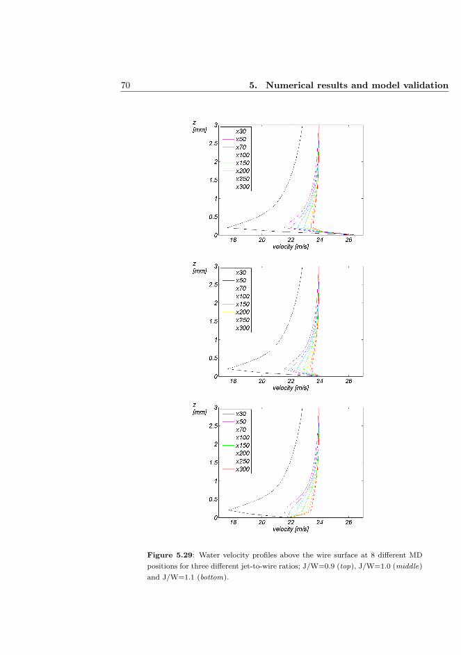
70 5. Numerical results and model validation
Figure 5.29: Water velocity profiles above the wire surface at 8 different MD
positions for three different jet-to-wire ratios; J/W=0.9 (top), J/W=1.0 (middle)
and J/W=1.1 (bottom).

5.3 Fibre flocculation in the forming section 71
Figure 5.30: Turbulent kinetic energy profiles above the wire surface at 8 differ-
ent MD positions for three different jet-to-wire ratios; J/W=0.9 (top), J/W=1.0
(middle) and J/W=1.1 (bottom).
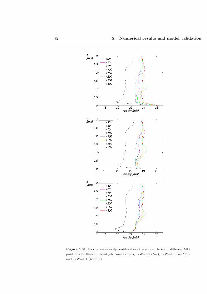
72 5. Numerical results and model validation
Figure 5.31: Floc phase velocity profiles above the wire surface at 8 different MD
positions for three different jet-to-wire ratios; J/W=0.9 (top), J/W=1.0 (middle)
and J/W=1.1 (bottom).

5.3 Fibre flocculation in the forming section 73
Figure 5.32: The initial dewatering occuring on the wire surface.
Figure 5.33: The mean floc diameter on the wire surface for three different
jet-to-wire ratios.
to the higher turbulent kinetic energy and higher shear. In Fig. 5.33 it can beseen that for the rush mode, the floc size on wire does not turn down before theposition x150 where the shear becomes important. However, the floc size does notdiminish significantly, but rather stays at the same level. For J/W=1.0 the flocsize increases continuously, since after the impingement there are no shear forcesor increase in the turbulent kinetic energy to break up the flocs. Further in thedownstream, i.e. at x250, the predicted floc size for J/W=1.0 seems somewhattoo big compared to the jet thickness. However, the model still correctly predictsthe fact that drag and rush modes are more efficient in the floc break up.

74 5. Numerical results and model validation
Figure 5.34: The impingement of the jet. The color represents the static pres-
sure.
Figure 5.35: The mean floc diameter inside the slice channel, in the free jet and
in the forming section, J/W=1.0.
The Fig. 5.33 gives only the information of the floc diameter on the wire surface,but it is interesting to look what happens in the jet thickness direction, and alsobefore the jet hits the moving wire. The Fig. 5.35 presents the countour plot ofthe development of the mean floc size in the slice channel, in the free jet and inthe very beginning of the forming section. The floc diameter is bigger betweenthe wedges than in their wakes as seen already when investigating the phenomenain the slice channel in Section 5.2.4. The z-directional difference in the local floc

5.3 Fibre flocculation in the forming section 75
size is carried far downstream in the jet, but it can be seen that the impingementzone has a remarkable effect on the local floc size: the mean floc size reducesinstantaneously at the proximity of the wire surface, while it remains practicallyuntouched at the upper surface of the jet.
In order to get more exact values of the floc diameters at different locationsover the jet thickness, the mean floc size is plotted along the black lines presentedin Fig. 5.35, that is, at the slice opening, at the end of the bottom lip and in thefree jet before it hits the wire surface. The profiles are depicted in Fig. 5.36, wherethe δ∗ represents the distance from the middle of the jet (δ∗ = 0 at the middle).The mean floc diameter is almost symmetrical at the slice opening; only the slightdeviation due to the slice bar can be distinguished. At the end of the bottom lipthe jet has already visibly contracted and the reduce in the mean floc size occureddue to the slice bar (at the top edge of the jet) can more clearly be seen. In the freejet, a little bit after the vena-contracta, the profile is not symmetrical anymore;the peak at the bottom lip side has significantly decreased, while the other peaksare only slightly smaller than before. However, based on the three graphs in Fig.5.36, it can be concluded that the contraction of the jet reduces the floc size dueto the velocity gradients and increased turbulent kinetic energy.
Figure 5.36: The mean floc diameter over the jet thickness at three different
MD positions: at the slice opening, at the end of the bottom lip and in the free
jet (The locations are illustrated in Fig. 5.35).
One drawback in the results in the forming section is that the local mean flocdiameter is 1 mm bigger at the end of the slice channel than observed in theSection 5.2.4, even though the slice channel is exactly the same. This is due to2D simplification: the model including the forming section assumes the even flowprofile in the CD direction, while in reality there is always a profile due to theturbulence generator. The 3D model used in the Section 5.2.4 takes this intoaccount, and hence, the floc size remains smaller. This inconvenience cannot be

76 5. Numerical results and model validation
avoided when using a 2D approach, and it may also explain too big floc size furtherin the forming section (Fig. 5.33).
Next, it is intresting to take a look at the development of the local mean flocdiameter at the forming section, where the phenomena are highly complex, Figs.5.37...5.40. At the impingement zone (Fig. 5.37) the profiles for all jet-to-wireratios are quite similar, only the middle peak seems higher for the rush mode.When proceeding further downstream, the simulations predict that the floc sizenear the free surface remains bigger for the rush case. This is quite interestingsuggestion, but due to the lack of the validation experiments, it is impossible tojudge the validity of that prediction. In addition, it has to be kept in mind thatpredicted floc sizes are too big because of the 2D simplification, and hence, it isbetter to concentrate in the local differencies occuring at different positions overjet thickness and in MD, and in comparison between the jet-to-wire ratios.
When investigating the near wire area in Fig. 5.38, it can be noticed that shearand turbulence start to break up flocs more efficiently for the drag mode than forother cases already at x100. For the rush mode, the effect of velocity gradientscan not be seen before x200 (Fig. 5.39), but when the effect takes place, it is quitestrong. The model suggests that the increase in the floc size occurs in the streaksformed already inside the slice channel, while in the wakes due to the wedge walls,the floc size would remain significantly smaller during the initial forming. In otherwords, the wedge walls cause turbulence and shear, which break up the flocs insidethe slice channel, and this effect is visible still in the initial dewatering zone. Asa consequence, the model suggests that the floc size, and the resulting formation,are different in separate layers in the forming paper.

5.3 Fibre flocculation in the forming section 77
Figure 5.37: The floc diameter on the wire surface through the jet thickness
at two different MD positions, x30 (top) and x50 (bottom), for three different
jet-to-wire ratios.
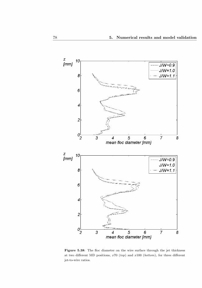
78 5. Numerical results and model validation
Figure 5.38: The floc diameter on the wire surface through the jet thickness
at two different MD positions, x70 (top) and x100 (bottom), for three different
jet-to-wire ratios.

5.3 Fibre flocculation in the forming section 79
Figure 5.39: The floc diameter on the wire surface through the jet thickness
at two different MD positions, x150 (top) and x200 (bottom), for three different
jet-to-wire ratios.

80 5. Numerical results and model validation
Figure 5.40: The floc diameter on the wire surface through the jet thickness
at two different MD positions, x250 (top) and x300 (bottom), for three different
jet-to-wire ratios.
Chapter 6
Future work and recommendations
Since a mathematical model is very seldom complete, some development ideasand remarks of current model assumptions are now summarised in this chapter.Hence, the purpose of this chapter is to provide insight into the strengths and theweaknesses of the models used.
As stated before, one common deficiency for both of the presented models, theFOPD and the FFE, is the modelling of the carrier phase turbulence. In principle,the turbulence could be accurately simulated for a one-phase Newtonian fluid,such as water, by using Direct Numerical Simulation (DNS), but it is too costlyCPU time-wise, and not capable to resolve industrial-scale geometries. Moreover,the presence of fibres makes the situation even more complex, since the fibrousphase affects turbulence by dampening certain scales - and it is not even knownwhich of them.
In addition, the drag forces between water and the fibrous phase determinevelocity differences between the phases. Traditionally, the drag force is accountedfor in the momentum equation of each phase by the drag coefficient, but reliabledefinitions for the coefficients of single fibres or non-spherical, deformable flocs donot exist.
Furthermore, as the concentration increases, fibre-fibre collisions take placeand should be included in the models. Here, we collide once again with thistrade-off between Lagrangian and Eulerian modelling approaches: modelling theeffects of fibre-fibre, or floc-floc, collisions with Eulerian approach requires alwaysconsiderable simplifications and assumptions. Therefore, the basic Eulerian two-phase flow modelling including four-way couplings (water-fibre and fibre-fibre, orwater-floc and floc-floc) should be further developed to carefully account for theinteractions.
Since the FOPD and FFE models are based on different assumptions, theirlimitations are separately presented in the following sections. Although they areboth used for describing the headbox and forming section phenomena in this thesis,their direct combining in the same model would not be recommended until furtherdevelopment is considered.
81

82 6. Future work and recommendations
6.1 Limitations and possibilities of the FOPD model
In the FOPD model the fibre suspension is considered so dilute that the fibre-fibre interactions can be ignored. Naturally, this is not true for typical wet endprocesses, which are aimed to be described in this, and many other, studies. Oneway to address this problem would be to perform micro-level simulations and derivethe macro-level interaction terms to Eulerian multi-phase flow models. Mortensenet al., for example, have studied the orientation of a single fibre in a turbulent flowby using DNS [74]. In their work, the flow of the carrying phase was fully resolvedand the fibre was assumed inflexible. In addition, in the recent doctoral thesisby Lindstrom, the fibre-level simulations were performed taking into account thefibre-fibre interactions [68]. Based on this kind of basic research, the macroscopicindustrial-level CFD modelling tools can be further developed.
One of the weak points of the FOPD model is the definition of the translationaland rotational diffusion coefficients. Some correlations based on the turbulentkinetic energy and dissipation are proposed in [84], but even the magnitude of thecoefficient is still a matter of debate, see eg. [51] and [78]. Thus, futher studies areneeded before the coefficients can be reliably determined.
Another serious drawback of the FOPD model is that it is derived for rigidfibres, or to be more accurate, for ellipsoidal particles. Wood fibres used in pulpand paper industry are, nevertheless, rather flexible, and their tendency to bealigned with the mean flow is not as strong as that of rigid fibres like seen in [78].In addition, the determination of the experimental orientation of a curly fibre isnot that unambiguous, and hence, the distributions can have quite a different formdepending on the method used.
For the sake of simplicity, the FOPD model is practically always used only tosimulate the projections of the fibre orientation angle; the one in (MD,CD)-planeor the one in (MD,z)-plane (see Fig. 3.1 for the clarification). However, the orien-tation of a fibre can, naturally, be the combination of these two angles, φ and θ. Inorder to study the resulting stratified orientation in a paper produced, one wouldneed to model the whole three-dimensional distribution. This would, however,lead to a five-dimensional modelling problem, and thus, some dimensional reduc-tion technique need to be applied to make the problem solvable for commercialCFD software.
The increasing pulp concentration involves the flocculation of fibres, which oc-curs even at relatively low concentrations [62]. Once the fibres are attached to afloc, their freedom to orient is strongly restricted, and after quick physical rea-soning, the FOPD should not provide any reliable information about the resultingorientation. However, it has been shown in [36] that even a much more simplemodel, basing on the MD and CD velocity components, produces results accurateenough for the paper machine control purposes. Thus, it can be summarised thatthe mean angle of fibre orientation is accurately predicted by relatively simpletools, but when needing the information about local variations, for example tostudy cockling, a more accurate model, such as the FOPD is required.

6.2 Limitations and possibilities of the FFE model 83
6.2 Limitations and possibilities of the FFE model
The basic population balance method is a solid basis for the flocculation modellingassuming that there are clearly higher and lower concentration regimes, i.e. fibreflocs and voids, in the flow. However, if all the fibres were part of one large fibrenetwork, (as can probably occur for high concenrations) the whole concept wouldbe questionable. On the other hand, for that kind of situation one does not usuallyeven talk about flocs. However, experiments have revealed the dynamics of the flocevolution for typical headbox concentrations [57], [97], and thus, the Fibre FlocEvolution (FFE) can be considered reasonable starting point for the flocculationmodelling.
As mentioned before, the break-up and coalescence models are originally de-veloped for gas-liquid flows. It was shown within the results of this thesis thatthose models offer an appropriate basis for the fibre flocculation modelling, butthe model parameters, and possibly whole the model kernels, need to be revised inorder to better describe the fibre suspension flows. The simulated results revealedthat the internal strength of a floc and the crowding factor of the pulp are corre-lated, and that further studies are needed to determine the physical dependencies.In this thesis the pulps differed by length, diameter and coarseness, but they wereof the same concentration. In addition, the floc strength was same for all differentfloc sizes, which may not be true. Since the strength of a floc is somehow corre-lated with the number of fibre-fibre bonds, it can be assumed that the internal flocstrength varies depending, at least, on the fibre properties, floc size and local flocdensity. Hence, more simulations and experiments would be needed to properlydefine the internal strength of a floc.
In regard to other modified model parameters, the break-up and the coalescencecoefficients, further research would be needed as well. In the model validation,they were kept constant, but it might occur that they should depend on pulpproperties, turbulence or other flow field properties. It is accentuated that thementioned parameters, if they turn out not to be constants, should be determinedsuch that the model is applicable to different geometries without any parametertuning, i.e. the parameters can depend on strain rate or turbulent kinetic energy,for instance, but not on the pipe diameter. As regards the other parameters,namely, the initial and the critical film thickness, they should also be determinedspecifically for fibre flocs.
The FFE model presented in this thesis has been validated only with one seriesof experiments including two different pulps, three different flow rates, but onlywith one type of geometry, namely the turbulence generator pipe. It is obviousthat the model should be validated in different geometries and for different pulpsand concentrations. It might occur that model parameters have to be completelyrevised in the future. However, the model provided at least qualitatively correctresults in the slice channel, which is the first indication that the FFE model is asuitable approach for the fibre flocculation modelling. To more reliably validatethe model parameters, more detailed experimental data is needed. For, now themeasurements have provided information of the floc size averaged over the whole

84 6. Future work and recommendations
pipe diameter, but in the future, data of the local floc size is required, since theflocculated state of the suspension varies considerably depending on the radiallocation, for example. This is most propably connected to the local properties ofthe flow field and turbulence.
In the current model, the turbulent conditions affect the break-up and coa-lescence mechanisms, but not vice versa. To more realisticly describe the fibresuspension flow, the turbulence modification due the prescence of flocs should beadded in the model, as discussed above. In addition, a number of other mecha-nisms, such as the erosion or attachement of a single fibre into a floc, have notbeen added in the FFE model.
The interactions between water and fibrous phase have been modelled withstandard type of drag laws developed for smooth, spherical and incompressibleparticles. The form of the floc is, nevertheless, far from those assumptions, andtherefore, fibre-water interactions are not correctly simulated. The form of a floccan change significantly depending on local flow conditions, and the compressibilityeffects take place especially in the forming section. The consolidation process isnot accounted for in this thesis, since it would require the definition of the fibrousphase as a totally different type of material. The phenomena in the forming sectionare, nonetheless, important when studying the forming of the fibrous structure ofpaper, and the effects of real porous wire as well as more detailed modelling ofdewatering and retention would give valuable information of the phenomena.
Finally, when looking at the flowing fibre suspension, one can notice that itsflocculated state is a sum of several factors, starting from the nature of the flowfield, ending to the influence of chemistry. Without no doubt, also the fibre orien-tation affects the flocculation, since more isotropically oriented fibres have morepossibilities to form bonds with neighbouring fibres. Consequently, the FOPDand the FFE models - or some of their more sophisticated descendants - shouldbe combined one day . This goal might seem distant and unattainable today, butwill most probably be achieved faster than we dare to believe.

Chapter 7
Conclusions
Ambitious goals to model the forming of the paper sheet by means of computa-tional fluid dynamics were stated in a research proposal filed to Finnish Academyin 2005. At that time fibre orientation modelling was under active research byseveral authors, but the fibre flocculation modelling had remained practically un-changed since the pioneering work of Steen in 1990’s. Both fibre orientation andflocculation were desired to be solved with a CFD tool available to industrialR&D. In other words, the research approach was to model complex phenomenasuch that it would be of intrest - and of use - in the industrial point of view. Thus,a commercial CFD software was chosen as a basis for the modelling work, and thesimulations were performed in geometries as close to real ones as possible.
Now, in this light, the thesis in your hands shows that the challenging objec-tives have been reached. The fibre orientation modelling has been performed inthe geometrically two-dimensional form in a headbox contraction, and the fibreflocculation modelling has been advanced to a completely new level, from Steen’sflocculation index to the concrete measurable floc sizes. This thesis is the firstproof that fibre flocculation can be studied by using the developed Fibre FlocEvolution (FFE) model based on the population balance of different floc sizes.Moreover, the FFE model creates a new basis to develop fibre suspension flowmodels in future, since the existence of two phases, water and fibrous phase, canbe taken into account, and also the local variation of flocculated state of suspensioncan be studied.
Furthermore, simulations were extended outside of the headbox, to the freejet and to the forming section, in order to predict paper sheet properties to someextent. The whole forming section was not studied in detail, but the effect of initialdewatering zone to the floc behaviour was inspected. The aim of the thesis wasnot to make any ”virtual paper sheet” by numerical simulations including billionsof fibres, or have an accurate estimation of the basis weight, but instead to givefluid dynamical insight in understanding how the paper sheet is formed.
Fibre orientation was studied in geometrically two-dimensional form, and in-cluding the slice channel and the contracting jet in simulations. The numerical
85
86 7. Conclusions
results revealed new phenomena, such as quick decrease of anisotropy in the freejet and two equally probable orientation angles at the slice opening. The fastdrop of anisotropy right after the slice opening proves the importance of includingthe free jet in the simulations, since the state of the orientation inside the slicechannel does not characterise the situation in the jet with enough reliability. Fur-ther, even though the secondary peak appearing at the slice opening fades outvery quickly, the existence of the peak proves that the FOPD model is capable topredict even very complicated phenomena. This would not be possible, if the one-dimensional formulation of the equation was used. Moreover, when investigatingthe orientation in the forming section one day, it is of utmost importance to havea model which is capable to simulate the behaviour of fibres submitted to complexphenomena at the jet impingement and during water removal.
Fibre flocculation was studied with a novel approach, the FFE model, whichis capable to predict real floc sizes. The model developed within this thesis givesintresting possibilities when developing further the theory of the behaviour of theflocculated state of the suspension. It enables also the comparison of geometricallydifferent constructions when designing parts of the headbox, since the model isrelatively easy to use, and hence, applicable in every-day R&D work.
The FFE model was validated in the turbulence generator, and it was thenused in investigation of the floc size behaviour in the slice channel and in theforming section. The floc size evolution in the slice channel was consistent withexperimental findings and common knowledge, and furthermore, the FFE modeloffered more detailed information than previous studies. It was noticed that theeffect of the turbulence generator pipe walls is visible far downstream, and alsothat the floc size is bigger in the middle of two wedges than near the wedge surface.The effect is inherited in the free jet and perceivable after the jet impingement aswell. The finding attests the importance of the design of the slice channel, sincethe small floc size due to the wedge wall generated turbulence remains in the jetand leads to better formation. Variation of the jet-to-wire speed ratio was alsoshown to modify the development of the mean floc size, which is consistent withcommon knowledge: the drag mode was predicted to most efficiently break up theflocs, while J/W=1.0 had the least effect.
A mathematical model is very seldom perfect, and thus, also in the FOPDand FFE models, many details are left for further investigations. It is worthwhileto remember that there are still unsolved problems in modelling turbulence evenin one-phase flow situations, and the presence of fibres does certainly not makeit any simpler. Concerning particularly turbulence in fibre suspension flows, themodelling - as well as experiments - have barely taken the first steps; clearlythe fibre concentration affects turbulence, but the interactions should be studiedin more detail. It is known that the prescence of fibres dampens certain scalesof turbulent fluctuations, but does the dampening occur similarly for differentfibre orientation distributions, or for different floc sizes? And further, fibre-fibreinteractions modify certainly the phenomena, especially, when going to higherconcentrations, but how?
The FFE model is a good basis to study the flocculation, but there is still

87
room for further development. For example, the erosion of flocs by separationof single fibres as well as attachment of single fibres to flocs have been left outof the current FFE model. In principle, the Eulerian multi-phase flow approachmakes it possible to include the erosion and attachment, but it means that thecarrying phase is not any more pure water, but a mixture of water and singlefibres. In addition, different floc sizes might have different strength properties,which affects the floc break-up mechanisms. Further, the chemistry; one essentialpart in the control of fluid mechanical phenomena in real papermaking process,and completely left away from the model. It is well recognised that retentionchemicals have a remarkable role in the paper sheet forming and in developmentof fibre-fibre bonds, but they are not tried to be included in the models of thisthesis.
In general, mathematical modelling and experimental measurements shouldbe developed hand in hand. Now the modelling has been advanced to a newlevel and next step waits for new experiments. Fibre orientation distributionsshould be measured in higher concentrations in order to validate and developthe FOPD model to better describe the practical applications. Also, fibre flocsize distributions should be measured instead of the average floc sizes in order tovalidate the FFE model more accurately, and to obtain valuable knowledge of thephenomenon itself.
The forming section modelling was simplified and only the initial dewateringof a Fourdrinier-type of former was studied. It would be intresting to extend thesimulations further in the forming section, and to model also a modern gap formerto see, how does the flocculation phenomenon differ in these two cases. Modellingthe moving wire as a real porous medium would give more accurate information ofthe floc size behaviour during the water removal, as well as including the blades,vacuum rolls and other dewatering components in simulations. Thus, there is anobvious demand for further modelling work, what comes to the floc size and ba-sis weight development in the whole forming section. And finally, the wet endfluid dynamical models could be linked to solid mechanical simulations in orderto really predict the strength properties and dimensional stability, and even finalend-use properties like printability of the paper sheet. Despite of the describedpotential development scenarios, already the current FFE model makes it pos-sible to perform accurate and detailed investigations of flocculation phenomenaand its dependency on different headbox and forming section design and runningparameters with utilising a commercial CFD tool available as well for academicalresearchers as for industrial R&D.

REFERENCES
[1] ANSYS CFX-11.0 electronical manual.[2] Advani S and Tucker C. The use of tensors to describe and predict fiber orientation
in short fiber composites. Journal of Rheology, 31:751–784, 1997.[3] Altan MC and Tang L. Orientation tensors in simple flows of dilute suspensions of
non-brownian rigid ellipsoids, comparison of analytical and approximate solutions.Rheologica acta, 32(3):227–244, 1993.
[4] Audenis G. On the impingement of a plane liquid jet on the wires of a papermachine. Licentiate thesis, Royal Institute of Technology, Stockholm, Sweden,1999.
[5] Audenis G and Dahlkild AA. Impingement of an inviscid plane liquid jet on aporous wall: A fixed domain method. Nordic Pulp and Paper Research Journal,16(4):274–283, 2001.
[6] Baines WD. The papriformer Part II. flow in the formation zone of a two-wiremachine. Pulp & Paper Canada, 68(10):T497–T505, 1967.
[7] Barratte C, Roux JC, Voillot C, Le Nest JF, Lonjont JC, and Mangin P. Simulationof initial fibre retention by forming fabric. In 54th Appita Annual Conference, pages415–420, Melbourne, Australia, 2000.
[8] Bennington CPJ, Kerekes RJ, and Grace JR. The yield stress of fibre suspensions.Canadian Journal of Chemical Engineering, 68:748–757, 1990.
[9] Bennington CPJ and Thangavel VK. The use of a mixing-sensitive chemical reac-tion for the study of pulp fibre suspension mixing. Canadian Journal of ChemicalEngineering, 71:667–675, 1993.
[10] Bergstrom R. Fibre flocculation during twin-wire roll forming. Licentiate thesis,Royal Institute of Technology, Stockholm, Sweden, 2003.
[11] Brecht W and Heller H. A study of the friction losses of paper stock suspensions.TAPPI Journal, 33(9):14A, 1950.
[12] Carlsson A. Orientation of fibres in suspensions flowing over a solid surface. Li-centiate thesis, Royal Institute of Technology, Stockholm, Sweden, 2007.
[13] Carlsson A, Lundell F, and Soderberg D. Fibre orientation control related topapermaking. Journal of Fluids Engineering, 129:457–465, 2007.
[14] Crowe C, Sommerfeld M, and Tsuji Y. Multiphase Flows with Droplets and Par-
88

References 89
ticles. CRC Press LLC, 1998.[15] Dalpke B, Green SI, and Kerekes RJ. Influence of machine variables on fibre mat
buildup at jet impingement. Journal of Pulp and Paper Science, 29(3):90–94, 2003.[16] Dalpke B and Kerekes RJ. The influence of fibre properties on the apparent
yield stress of flocculated pulp suspensions. Journal of Pulp and Paper Science,31(1):39–43, 2005.
[17] Dalpke B, Kerekes RJ, and Green SI. Modelling jet impingement and the initialdrainage zone in roll forming. Journal of Pulp and Paper Science, 30(3):65–70,2004.
[18] Deng C and Martinez DM. Towards an understanding of the flow at the egde of aporous medium. Journal of Pulp and Paper Science, 32(4):1–6, 2006.
[19] Deng M and Dodson CTJ. Random star patterns and paper formation. TAPPIJournal, 77(3):195–199, 1994.
[20] Dodson CTJ. Fibre crowding, fibre contacts and fibre flocculation. TAPPI Journal,79(9):211–216, 1996.
[21] Dodson CTJ and Kerekes RJ. On the structure of fibre flocs. Technical report,Presented at the COST Meeting on Multi-Phase Flows in Papermaking, Grenoble,1997.
[22] Dodson CTJ and Serafino L. Flocculation, dispersion and dynamic scenarios forformation. Nordic Pulp and Paper Research Journal, 8(2):264–272, 1993.
[23] Eloranta H. Estimation of fiber orientation in pulp-suspension flow. In 3rd In-ternational Symposium on Two-Phase Flow Modelling and Experimentation, Pisa,2004.
[24] Erkkila AL, Pakarinen P, and Odell M. Sheet forming studies using layered orien-tation analysis. Pulp Paper Canada, 99(1):81–85, 1998.
[25] Farnood RR, Dodson CTJ, and Loewen SR. Modelling flocculation. part i: Ran-dom disc model. Journal of Pulp and Paper Science, 21(10):J348–355, 1995.
[26] Farnood RR, Loewen SR, and Dodson CTJ. Estimation of intra-floc forces. AP-PITA Journal, 47(5):391–396, 1994.
[27] Farnood RR, Yan N, Kortschot MT, and Dodson CTJ. Modelling flocculation: Agallery of simulated flocculated papers. Nordic Pulp and Paper Research Journal,12(2):86–89, 1997.
[28] Garner RG and Kerekes RJ. Measurement of turbulence in pulp suspension bylaser anemometry. Trans. Tech. Sect. CPPA, 8(3):TR53–69, 1982.
[29] Gidaspow D. Multiphase Flow and Fluidization. Academic Press, 1994.[30] Gorres J, Cresson T, and Luner P. Sheet formation from flocculated structures.
Journal of Pulp and Paper Science, 15(2):55–59, 1989.[31] Gullichsen J. Chemical engineering principles of fiber line operations. In Gullich-
sen J and Fogelholm CJ, editors, Chemical Pulping, volume 6A of PapermakingScience and Technology, pages A245–A327. Fapet Oy, Helsinki, Finland, 1999.
[32] Gullichsen J and Harkonen E. Medium consistency technology. II. storage dis-chargers and centrifugal pumps. TAPPI Journal, 64:113–116, 1981.
[33] Hamalainen J. Mathematical Modeling and Simulation of Fluid Flows in the Head-box of Paper Machines. PhD thesis, University of Jyvaskyla, 1993.
[34] Hamalainen J, Hamalainen T, Madetoja E, and Ruotsalainen H. CFD-based op-timization for complete industrial process: Papermaking. In Thevenin D andJaniga G, editors, Optimization and Computational Fluid Dynamics. Springer,2008.
[35] Hamalainen J and Tarvainen P. CFD-based shape and control optimization applied

90 References
to a paper machine headbox. In 86th ann. meeting of PAPTAC, pages A99–A102,2000.
[36] Hamalainen J, Tarvainen P, and Aspholm P. HOCS FIBRE – new tool for opti-mized fibre orientation angles. In 91st ann. meeting of PAPTAC, CD-proceedings,2005.
[37] Hamalainen T and Hamalainen J. Modelling of fibre orientation in the headboxjet. Journal of Pulp and Paper Science, 33(1):49–53, 2007.
[38] Hamalainen T, Hamalainen J, and Salmela J. Evolution of fibre flocs in a turbulentpipe expansion flow. In 6th International Conference on Multiphase Flow (CD-proceedings), 2007.
[39] Hammarstrom D. A model for simulation of fiber suspension flows. Licentiatethesis, Royal Institute of Technology, Stockholm, Sweden, 2004.
[40] Hiltunen K. Mathematical and numerical modelling of consolidation processes inpaper machines. PhD thesis, University of Jyvaskyla, Finland, 1995.
[41] Hinze JO. Turbulence. McGraw-Hill, New York, 1959.[42] Holm R. Fluid Mechiancs of Fibre Suspensions Related to Papermaking. PhD
thesis, Royal Institute of Technology, Stockholm, Sweden, 2005.[43] Holmqvist C. Mechanical Modelling of Blade Forming and Drainage of Flocculated
Suspensions. PhD thesis, Royal Institute of Technology, Stockholm, Sweden, 2005.[44] Hourani MJ. Fiber flocculation in pulp suspension: Part 1: Theoretical model.
TAPPI Journal, 71(5):115–118, 1988.[45] Huber P, Roux JC, Mauret E, Belgacem N, and Pierre C. Suspension crowding for
a general fibre-length distribution: Application to flocculation of mixtures of shortand long papermaking fibres. Journal of Pulp and Paper Science, 29(3):77–85,2003.
[46] Huhtanen JP. Modeling of Fiber Suspension Flows in Refiner and other Paper-making Processes by Combining Non-Newtonian Fluid Dynamics and Turbulence.PhD thesis, Tampere University of Technology, Finland, 2004.
[47] Hyensjo M. On fibre suspension flow modelling: Mechanical fibre flocculationand fibre orientation. Licentiate thesis, Royal Institute of Technology, Stockholm,Sweden, 2005.
[48] Hyensjo M. Fibre Orientation Modelling Applied to Contracting Flows Relatedto Papermaking. PhD thesis, Royal Institute of Technology, Stockholm, Sweden,2008.
[49] Hyensjo M, Dahlkild A, Krochak P, Olson J, and Hamalainen J. Modelling theeffect of shear flow on fibre orientation anisotropy in a planar contraction. NordicPulp and Paper Research Journal, 22(3):376–382, 2007.
[50] Hyensjo M, Hamalainen J, and Dahlkild A. Turbulent dilute fibre suspension flowmodelling in a sudden circular pipe enlargement. In 89th annual meeting of Pulpand Paper Technical Association of Canada (CD proceedings). Springer, 2003.
[51] Hyensjo M, Krochak P, Olson J, Hamalainen J, and Dahlkild A. Modelling aturbulent dilute fibre suspension in a planar contraction: Effect of vane types,vane position and wall boundary layer on fibre orientation distribution. In 5th Int.Conf. on Multiphase Flow, ICMF’04, Yokohama, Japan, 2004.
[52] James DF, Yogachandran N, Loewen MR, Liu H, and Davis AMJ. Floc rupturein extensional flow. Journal of Pulp and Paper Science, 29(11):377–382, 2003.
[53] Jeffery GB. The motion of ellipsoidal particles immersed in a viscous fluid. Proc.Royal Soc., A102:161–179, 1923.
[54] Jetsu P, Kellomaki M, Karema H, Salmela J, Lappalainen T, and Piirto M. Co-

References 91
herent structures of suspension flow and their inheritance in paper. In 12th Fun-damental Research Symposium, Oxford, September 2001.
[55] Jokinen O and Ebeling K. Flocculation tendency of papermaking fibers. Paperija Puu, 67(5):317–325, 1985.
[56] Jong JH. Characteristics of Jet Impingement, Drainage and Compression in aForming Roll of a Twin-Wire Machine. PhD thesis, University of Toronto, Canada,1998.
[57] Karema H, Salmela J, Tukiainen M, and Lepomaki H. Prediction of paper forma-tion by fluidisation and reflocculation experiments. In 12th Fundamental ResearchSymposium, pages 559–589, 2001.
[58] Kerekes RJ. Flocculation in decaying turbulence: A literature review. Journal ofPulp and Paper Science, 9(3):TR86–91, 1983.
[59] Kerekes RJ. Pulp floc behavior in entry flow to constrictions. TAPPI Journal,66(1):88–91, 1983.
[60] Kerekes RJ and Schell CJ. Characterization of fibre flocculation regimes by acrowding factor. Journal of Pulp and Paper Science, 18(1):32–38, 1992.
[61] Kerekes RJ and Schell CJ. Effects of fibre length and coarseness on pulp floccula-tion. TAPPI Journal, 78(2):133–139, 1995.
[62] Krochak PJ, Olson J, and Martinez DM. The orientation of semidiluterigid fiber suspensions in a linearly contracting channel. Physics of Fluids,20(7):DOI:10.1063/1.2949277, 2008.
[63] Kropholler HW and Sampson WW. The effect of fibre length distribution onsuspension crowding. Journal of Pulp and Paper Science, 27(9):301–305, 2001.
[64] Kuhn DCS and P. Sullivan PE. Analysis and measurement of the flocculationintensity of flowing pulp suspensions. In TAPPI Papermakers Conference (CDproceedings), Cincinnati, OH, USA, 2001.
[65] Launder BE and Sharma BI. Application of the energy-dissipation model of tur-bulence to the calculation of flow near a spinning disc. Letters in Heat and MassTransfer, 1(2):131–138, 1974.
[66] Lee PFW and Duffy GG. Analysis of the drag reducing regime of pulp suspension.TAPPI Journal, 59:119–122, 1976.
[67] Leppanen T. Effect of Fiber Orientation on Cockling of Paper. PhD thesis, Uni-versity of Kuopio, Finland, 2007.
[68] Lindstrom SB. Modelling and Simulation of Paper Structure Development. PhDthesis, Mid Sweden University, Sundsvall, Sweden, 2008.
[69] Ljus C. On Particle transport and turbulence modification in air particle flows.PhD thesis, Chalmers University of Technology, Sweden, 2000.
[70] Luo H and Svendsen HF. Theoretical model for drop and bubble breakup inturbulent dispersions. AIChE Journal, 42(5):1225–1233, 1996.
[71] Martinez DM, Kiiskinen H, Ahlman AK, and Kerekes RJ. On the mobility offlowing papermaking suspensions and its relationship to formation. Journal ofPulp and Paper Science, 20(10):341–347, 2003.
[72] Mason SG. Fibre motion and floccation. Pulp and Paper Magazine of Canada,55(13):96–102, 1954.
[73] Melander O. Fluid dynamics and flow structures of wood fibres suspended in gasflows. PhD thesis, Chalmers University of Technology, Sweden, 2006.
[74] Mortensen PH, Andersson HI, Gillissen JJJ, and Boersma BJ. On the orientation ofellipsoidal particles in a turbulent shear flow. International Journal of MultiphaseFlow, 34(7):678–683, 2008.
92 References
[75] Myreen B. Modeling the flow of pulp suspensions in pipes, part i. Paperi ja Puu,5:497–504, 1989.
[76] Niemisto A, Hiltunen K, and Hamalainen J. Fluid-structure interaction andfree surface problems in papermaking process. In ECCOMAS 2000 conference,Barcelona, Spain, 2000.
[77] Niskanen H and Hamalainen J. Modelling of fibre orientation in a paper machineheadbox geometry. In 21st Nordic Seminar on Computational Mechanics, pages139–142, 2008.
[78] Niskanen H, Hamalainen T, Eloranta H, Vaittinen J, and Hamalainen J. De-pendence of fibre orientation on turbulence of the headbox flow. In 94th AnnualMeeting of PAPTAC, CD-proceedings, pages B339–B342, 2008.
[79] Niskanen K, Kajanto I, and Pakarinen P. Fibre orientation. In Niskanen K, editor,Paper Physics, volume 16 of Papermaking Science and Technology, pages 37–50.Fapet Oy, Helsinki, Finland, 1998.
[80] Norman B. Overview of the physics of forming. In 9th Fundamental ResearchSymposium, pages 73–149, Cambridge, 1989.
[81] Norman B. Letter to the editor. Nordic Pulp and Paper Research Journal,12(3):210, 1997.
[82] Norman B, Moller K, Ek R, and Duffy G. Hydrodynamics of papermaking fibresin water suspension. In Fibre-Water Interactions in Paper-Making, pages 195–250,Oxford, 1977.
[83] Norman B and Soderberg D. Overview of forming literature: 1990-2000. In 12thFundamental Research Symposium, pages 431–558, Oxford, 2001.
[84] Olson JA. The motion of fibres in turbulent flow, stochastic simulation of isotropichomogeneous turbulence. International Journal of Multiphase Flow, 27:2083–2103,2001.
[85] Olson JA, Frigaard I, Chan C, and Hamalainen J. Modeling a turbulent fibresuspension flowing in a planar contraction: The one-dimensional headbox. Inter-national Journal of Multiphase Flow, 30:51–56, 2004.
[86] Olson JA and Kerekes RJ. The motion of fibres in turbulent flow. InternationalJournal of Multiphase Flow, 377:47–64, 1998.
[87] Parsheh M. Flow in Contractions with Applications to Headboxes. PhD thesis,Royal Institute of Technology, Stockholm, Sweden, 2001.
[88] Parsheh M and Dahlkild A. Modelling the flow around elastic guiding vanes inthe converging zone of a headbox. In TAPPI Engineering/Process and ProductQuality Conference, pages 1433–1452, Anaheim, USA, 1999.
[89] Paulapuro H, editor. Papermaking, Part 1, Stock Preparation and Wet End. Num-ber 8 in Papermaking Science and Technology. Fapet, Helsinki, 2000.
[90] Plikas A, Kuhn DCS, and P. Sullivan PE. A numerical model of fibre suspensionsin a grid generated turbulent flow. In ASME 2000 Fluids Engineering DivisionSummer Meeting: Proceedings of ASME FEDSM’00, pages 991–996, Boston, Mas-sachusetts, USA, 2000.
[91] Pope SB. Turbulent Flows. Cambridge University Press, Cambridge, 2000.[92] Pourahmadi F and Humphrey JAC. Modeling solid-fluid turbulent flows with
application to predicting erosive wear. PhysicoChemical Hydrodynamics, 4:191–219, 1983.
[93] Prince MJ and Blanch HW. Bubble coalescence and break-up in air-sparged bubblecolumns. AIChE Journal, 36(10):1485–1499, 1990.
[94] Raghem-Moayed A. Characterisation of Fibre Suspension Flows at Papermaking

References 93
Consistencies. PhD thesis, University of Toronto, Canada, 1999.[95] Raghem-Moayed A and Kuhn D. Turbulent flocculation measurement. Journal of
Pulp and Paper Science, 26(4):163–165, 2000.[96] Ramkrishna D. Population Balances - Theory and Applications to Particulate
Systems in Engineering. Academic Press, San Diego, 2000.[97] Salmela J and Kataja M. Floc rupture and re-flocculation in turbulent shear flow.
In 13th Fundamental Research Symposium, pages 35–50, 2005.[98] Sampson WW, McAlpin J, Kropholler HW, and Dodson CTJ. Hydrodynamic
smoothing in the sheet forming process. Journal of Pulp and Paper Science,21(12):J422–426, 1995.
[99] Schiller L and Naumann Z. A drag coefficient correlation. Z. Ver. Deutsch. Ing.,77:318, 1935.
[100] Schmid CF, Switzer LH, and Klingenberg D. Simulation of fiber flocculation: Effectof fiber properties and interfiber friction. Journal of Rheology, 44(4):781–809, 2000.
[101] Shakespeare J. Tutorial: Fibre orientation angle profiles - process principles andcross machine control. In TAPPI-proceedings, Process Contol, Electrical & Infor-mation Conference, pages 593–636, 1998.
[102] Shanker R, Gillespie Jr. JW, and Guceri SI. On the effect of nonhomogenous flowfields on the orientation distribution and rheology of fiber suspensions. Polym.Eng. Sci., 31:161–171, 1991.
[103] Shimizu T, Yokogawa A, Suzuki M, and Nakamura I. Study on flow character-istics of pulp suspension: 2nd report - flocculation measurements of a thick fibersuspension. Bulletin JSME, 29:1487–1493, 1986.
[104] Smith MK. Formation potential of west coast kraft pulps. Pulp & Paper Canada,87(10):69–76, 1986.
[105] Soderberg D. Experimental and theoretical studies of plane liquid jets. Licentiatethesis, Royal Institute of Technology, Stockholm, Sweden, 1997.
[106] Soderberg D. Hydrodynamics of a plane liquid jet aimed at applications in paper-manufacturing. PhD thesis, Royal Institute of Technology, Stockholm, Sweden,1999.
[107] Soszynski RM. The Formation and Properties of Coherent Flocs in Fibre Suspen-sions. PhD thesis, University of British Columbia, Canada, 1987.
[108] Steen M. Turbulence and Flocculation in Fibre Suspensions. PhD thesis, Universityof Trondheim, 1990.
[109] Switzer LH and Klingenberg DJ. Flocculation in simulations of sheared fibersuspensions. International Journal of Multiphase Flow, 30:67–87, 2004.
[110] Tennekes H and Lumley JL. A First Course in Turbulence. The MIT Press,Cambridge, MA, 1972.
[111] Tornberg A and Shelley MJ. Simulating the dynamics and interactions of flexiblefibers in Stokes flows. J. Comput. Phys., 196:8–40, 2004.
[112] Ullmar M. On fibre alignment mechanics in a headbox nozzle. Licentiate thesis,Royal Institute of Technology, Stockholm, Sweden, 1998.
[113] Wahren D. Fiber network structures in papermaking operations. In Institute ofPaper Chemistry Symposium ’Paper Science and Technology - The Cutting Edge’,pages 112–129, Appleton, WI, 1977.
[114] Wikstrom T. Flow and Rheology of Pulp Suspensions at Medium Consistency. PhDthesis, Chalmer’s University of Technology, Sweden, 2002.
[115] Wikstrom T and Rasmuson A. Yield stress of pulp suspensions: The influenceof fibre properties and processing conditions. Nordic Pulp and Paper Research

94 References
Journal, 13(3):243–250, 1998.[116] Xu HJ and Aidun CK. Characteristics of fiber suspension flow in a rectangular
channel. International Journal of Multiphase Flow, 31:318–336, 2005.[117] Yokogawa A, Suzuki M, and Shimizu T. Study on flow characteristics of pulp
suspension flow - measurement of turbulence intensity and fiber concentration un-evenness. Bulletin JSME, 28:846–853, 1985.
[118] Zahrai S. On the Fluid Mechanics of Twin-Wire Formers. PhD thesis, RoyalInstitute of Technology, Stockholm, Sweden, 1997.
[119] Zhao R and Kerekes RJ. Pressure distribution between forming fabrics in bladegap formers: Thin blades. Journal of Pulp and Paper Science, 21(3):97–103, 1995.