Normalized power spectrum analysis based on Linea ... · Normalized power spectrum analysis based...

Normalized power spectrum analysis based on Linea Prediction Code (LPC) using time integral procedures

Kazuo MURAKAWA†, Hidenori ITO

†, Masao MASUGI

†, Hitoshi KIJIMA

†††

† Technical Assistance and support center

NTT East

1-2-5 Kamata-honcho, Ohta-ku, Tokyo, 140-0053

JAPAN

[email protected]

†† Electric and Electronic Department

Ritsumeikan University,

1-1-1 Ichinomitihigashi, Kusatsu-shi, Siga, 525- 8577

JAPAN

[email protected]

††† Electrical Department

Polytechnic University

2-32-1 Ogawanishi, Kodaira, Tokyo, 187-0035

JAPAN

[email protected]

Abstract: - Recently malfunctions of telecommunication installations caused by switching noises of electric

equipment or devices have been increasing. The switching noises usually have low frequency components less

than 50Hz and also more than 9kHz or 150 kHz. It is useful to detect power spectrum of noises in order to solve

EMC problems. The LPC (Linear Prediction Code) method is known as a powerful frequency estimation

method. This paper proposes a new normalized power spectrum analysis technique based on LPC. Introducing

time integration on a time series of the noise waves to the LPC shows that noise power spectrum (frequencies

and levels) can be estimated more precisely than using the conventional LPC method. Estimated deviations of

frequency and NPS (normalized power spectrum) between given frequencies and extracted frequencies of quasi

signals are less than 4%, and the proposed technique can also extract low frequencies with short durations from

time series of noises.

Key-Words: - LPC (Linear prediction code), frequency analysis, time integral, simulations and

experiments

WSEAS TRANSACTIONS on COMMUNICATIONS Kazuo Murakawa, Hidenori Ito, Masao Masugi, Hitoshi Kijima

E-ISSN: 2224-2864 452 Volume 13, 2014

1 Introduction

Reducing CO2 emissions by minimizing

equipment power consumption is one of the more

important issues in the world. There are many ways

to reduce CO2 emissions, such as increasing power

circuit efficiency, reducing power consumption

itself, and using sleep modes. It is common

knowledge that solar, wind and geothermal power

systems have low CO2 emissions. One way to

reduce equipment CO2 emissions is to increase the

efficiency of ac/dc convertors. For this purpose

switching power circuits are used in both

telecommunication installations and power systems.

Initially, switching frequencies were in the range of

few kHz, but now switching frequencies in the

range of 9 to 150 kHz are used in order to increase

efficiency and downsize power circuits, particularly

frequency transformers. A side effect is that these

power circuits become a source of electromagnetic

noise with a wide frequency range. This power

spectrum noise causes malfunctions of equipment

connected to ac power mains [1].

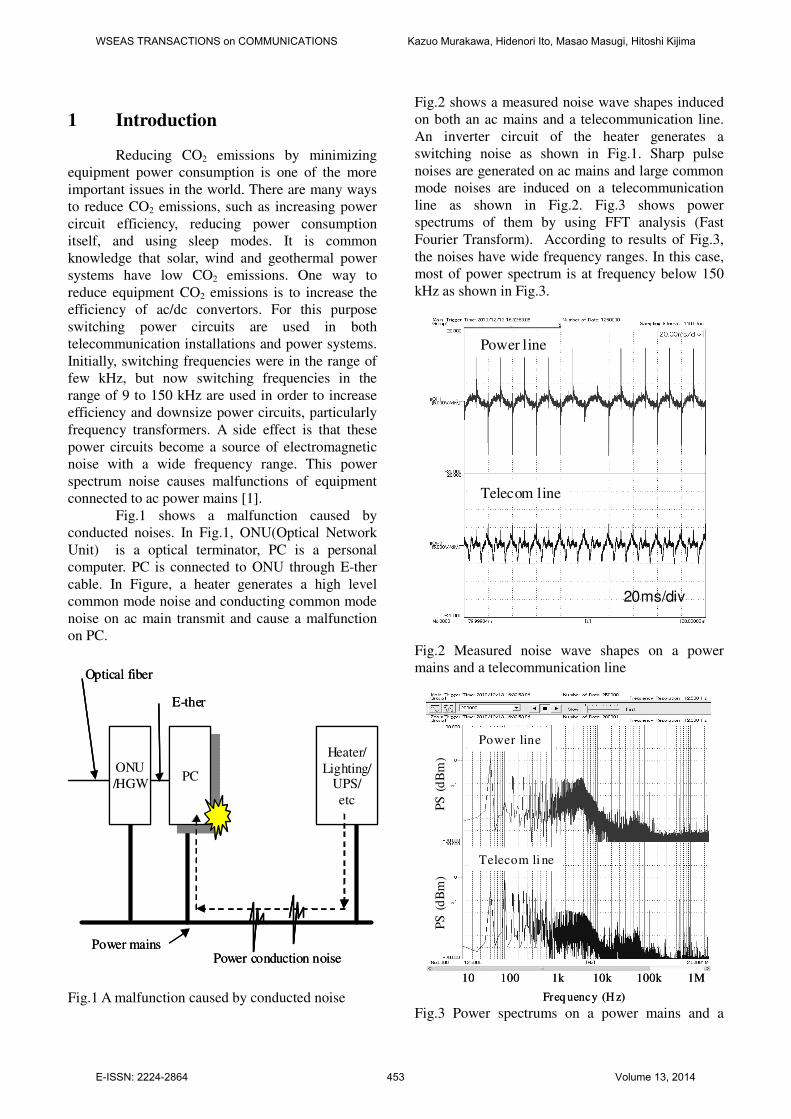
Fig.1 shows a malfunction caused by

conducted noises. In Fig.1, ONU(Optical Network

Unit) is a optical terminator, PC is a personal

computer. PC is connected to ONU through E-ther

cable. In Figure, a heater generates a high level

common mode noise and conducting common mode

noise on ac main transmit and cause a malfunction

on PC.

ONU

/HGW PCPC

Heater/

Lighting/UPS/

etc

Power mainsPower conduction noise

Optical fiber

E-ther

ONU

/HGW PCPC

Heater/

Lighting/UPS/

etc

Power mainsPower conduction noise

Optical fiber

E-ther

Fig.1 A malfunction caused by conducted noise

Fig.2 shows a measured noise wave shapes induced

on both an ac mains and a telecommunication line.

An inverter circuit of the heater generates a

switching noise as shown in Fig.1. Sharp pulse

noises are generated on ac mains and large common

mode noises are induced on a telecommunication

line as shown in Fig.2. Fig.3 shows power

spectrums of them by using FFT analysis (Fast

Fourier Transform). According to results of Fig.3,

the noises have wide frequency ranges. In this case,

most of power spectrum is at frequency below 150

kHz as shown in Fig.3.

Power line

Telecom line

20ms/div

Power line

Telecom line

20ms/div

Fig.2 Measured noise wave shapes on a power

mains and a telecommunication line

- 70+ 300

Freq uency (H z)

10 100 1k 10k 100k 1M-+ 300

Power line

Telecom li ne

PS

(d

Bm

)P

S (

dB

m)

- 70+ 300

Freq uency (H z)

10 100 1k 10k 100k 1M-+ 300

Power line

Telecom li ne

PS

(d

Bm

)P

S (

dB

m)

Fig.3 Power spectrums on a power mains and a


E-ISSN: 2224-2864 453 Volume 13, 2014

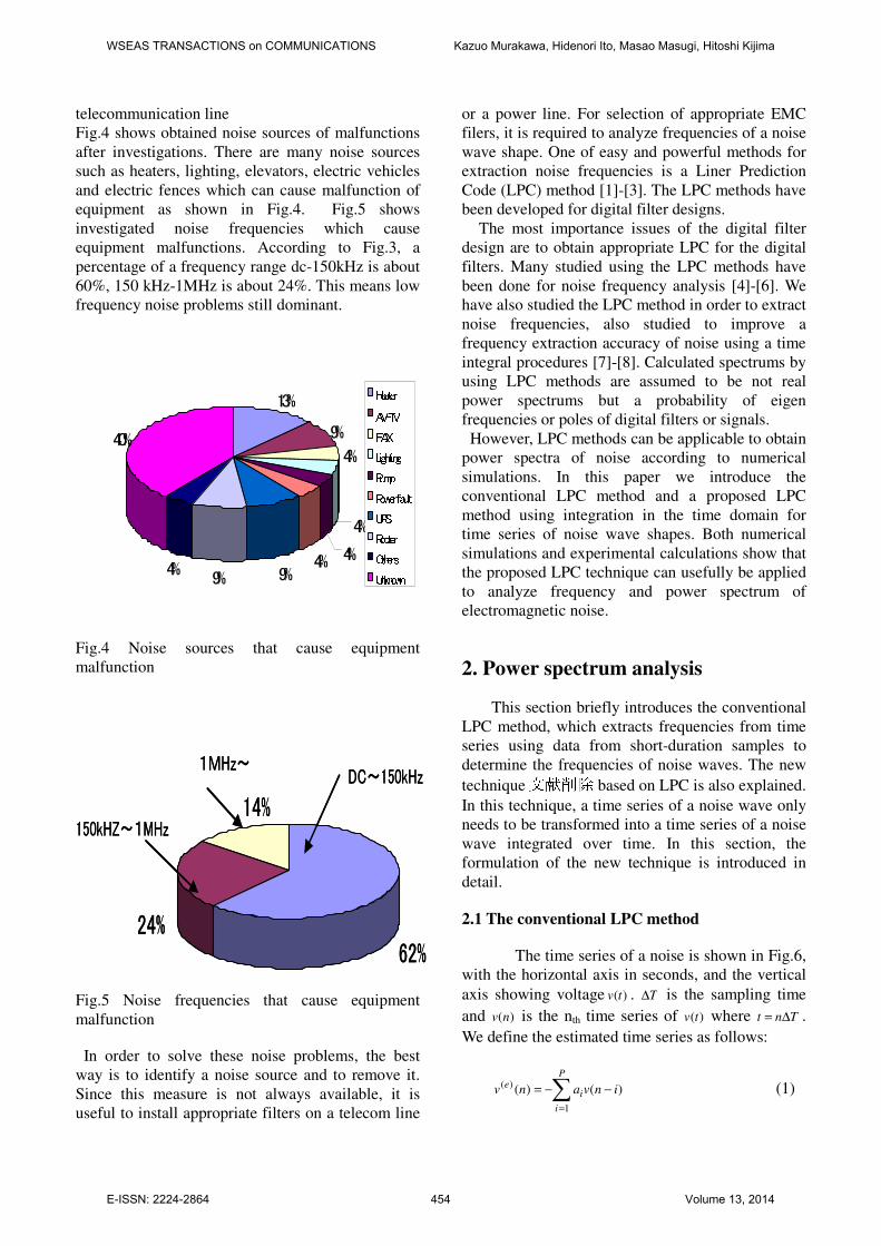
telecommunication line

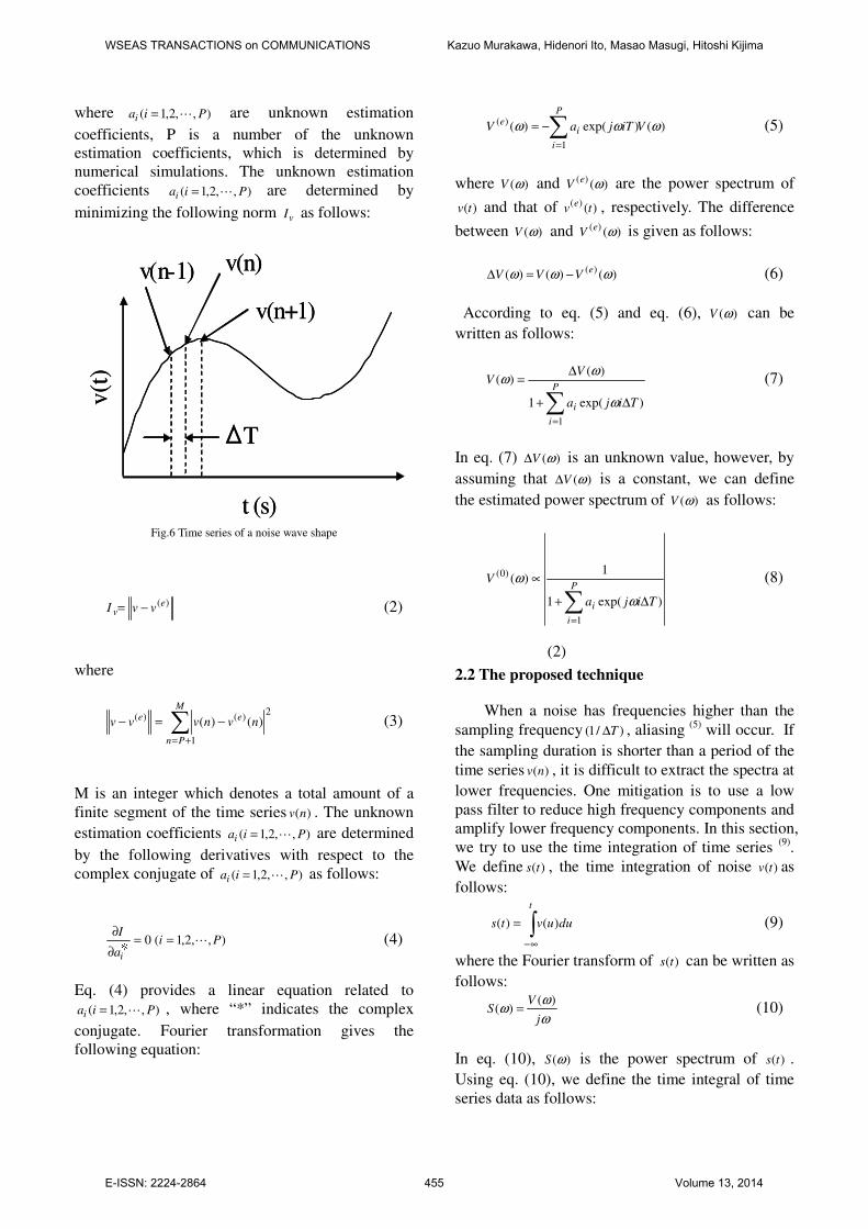
Fig.4 shows obtained noise sources of malfunctions

after investigations. There are many noise sources

such as heaters, lighting, elevators, electric vehicles

and electric fences which can cause malfunction of

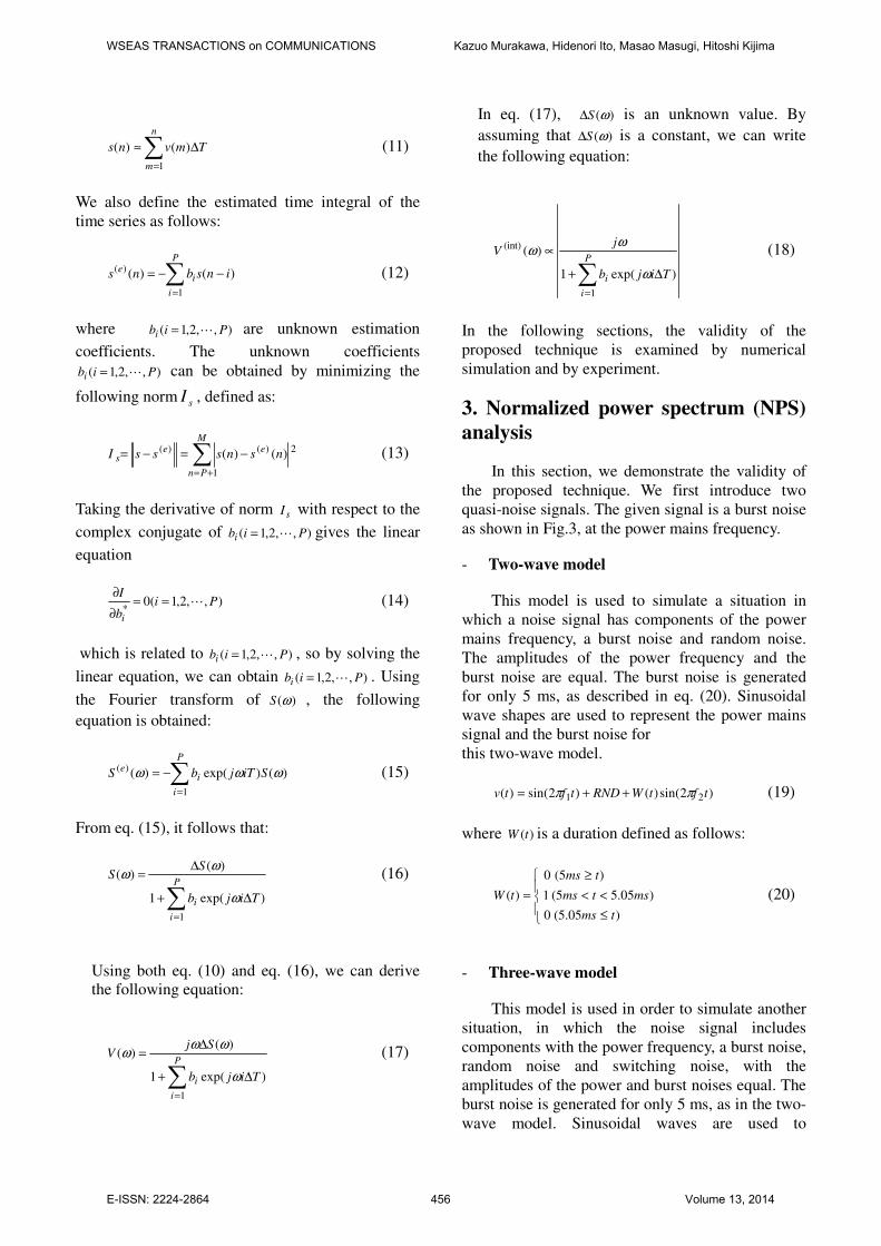
equipment as shown in Fig.4. Fig.5 shows

investigated noise frequencies which cause

equipment malfunctions. According to Fig.3, a

percentage of a frequency range dc-150kHz is about

60%, 150 kHz-1MHz is about 24%. This means low

frequency noise problems still dominant.

13%

9%

4%

4%

4%

4%

9%9%

4%

40%

HeaterAV-TVＦＡＸLightingPumpPower faultUPSRooterOthersUnknown13%

9%

4%

4%

4%

4%

9%9%

4%

40%

HeaterAV-TVＦＡＸLightingPumpPower faultUPSRooterOthersUnknown

Fig.4 Noise sources that cause equipment

malfunction

24%

14%

62%

DC～150kHz

150kHZ～１MHz

１ＭHz～

24%

14%

62%

DC～150kHz

150kHZ～１MHz

１ＭHz～

Fig.5 Noise frequencies that cause equipment

malfunction

In order to solve these noise problems, the best

way is to identify a noise source and to remove it.

Since this measure is not always available, it is

useful to install appropriate filters on a telecom line

or a power line. For selection of appropriate EMC

filers, it is required to analyze frequencies of a noise

wave shape. One of easy and powerful methods for

extraction noise frequencies is a Liner Prediction

Code (LPC) method [1]-[3]. The LPC methods have

been developed for digital filter designs. The most importance issues of the digital filter

design are to obtain appropriate LPC for the digital

filters. Many studied using the LPC methods have

been done for noise frequency analysis [4]-[6]. We

have also studied the LPC method in order to extract

noise frequencies, also studied to improve a

frequency extraction accuracy of noise using a time

integral procedures [7]-[8]. Calculated spectrums by

using LPC methods are assumed to be not real

power spectrums but a probability of eigen

frequencies or poles of digital filters or signals.

However, LPC methods can be applicable to obtain

power spectra of noise according to numerical

simulations. In this paper we introduce the

conventional LPC method and a proposed LPC

method using integration in the time domain for

time series of noise wave shapes. Both numerical

simulations and experimental calculations show that

the proposed LPC technique can usefully be applied

to analyze frequency and power spectrum of

electromagnetic noise.

2. Power spectrum analysis

This section briefly introduces the conventional

LPC method, which extracts frequencies from time

series using data from short-duration samples to

determine the frequencies of noise waves. The new

technique文献削除 based on LPC is also explained.

In this technique, a time series of a noise wave only

needs to be transformed into a time series of a noise

wave integrated over time. In this section, the

formulation of the new technique is introduced in

detail.

2.1 The conventional LPC method

The time series of a noise is shown in Fig.6,

with the horizontal axis in seconds, and the vertical

axis showing voltage )(tv . T∆ is the sampling time

and )(nv is the nth time series of )(tv where Tnt ∆= .

We define the estimated time series as follows:

∑=

−−=

P

i

ie invanv

1

)( )()( (1)


E-ISSN: 2224-2864 454 Volume 13, 2014

where ),,2,1( Piai L= are unknown estimation

coefficients, P is a number of the unknown

estimation coefficients, which is determined by

numerical simulations. The unknown estimation

coefficients ),,2,1( Piai L= are determined by

minimizing the following norm vI as follows:

v(t

)

t (s)

v(n)

v(n+1)

v(n-1)

ΔT

v(t

)

t (s)

v(n)

v(n+1)

v(n-1)

ΔT

Fig.6 Time series of a noise wave shape

)(e

v vvI −= (2)

(2)

where

∑+=

−=−

M

Pn

ee nvnvvv

1

2)()( )()( (3)

M is an integer which denotes a total amount of a

finite segment of the time series )(nv . The unknown

estimation coefficients ),,2,1( Piai L= are determined

by the following derivatives with respect to the

complex conjugate of ),,2,1( Piai L= as follows:

),,2,1(0 Pia

I

i

L==∂

∂＊ (4)

Eq. (4) provides a linear equation related to

),,2,1( Piai L= , where “*” indicates the complex

conjugate. Fourier transformation gives the

following equation:

)()exp()(

1

)( ωωω ViTjaV

P

i

ie ∑

=

−= (5)

where )(ωV and )()( ωe

V are the power spectrum of

)(tv and that of )()(

tve , respectively. The difference

between )(ωV and )()( ωe

V is given as follows:

)()()()( ωωω e

VVV −=∆ (6)

According to eq. (5) and eq. (6), )(ωV can be

written as follows:

∑=

∆+

∆=

P

i

i Tija

VV

1

)exp(1

)()(

ω

ωω (7)

In eq. (7) )(ωV∆ is an unknown value, however, by

assuming that )(ωV∆ is a constant, we can define

the estimated power spectrum of )(ωV as follows:

∑=

∆+

∝P

i

i Tija

V

1

)0(

)exp(1

1)(

ω

ω (8)

2.2 The proposed technique

When a noise has frequencies higher than the

sampling frequency )/1( T∆ , aliasing (5)

will occur. If

the sampling duration is shorter than a period of the

time series )(nv , it is difficult to extract the spectra at

lower frequencies. One mitigation is to use a low

pass filter to reduce high frequency components and

amplify lower frequency components. In this section,

we try to use the time integration of time series (9)

.

We define )(ts , the time integration of noise )(tv as

follows:

∫∞−

=

t

duuvts )()( (9)

where the Fourier transform of )(ts can be written as

follows:

ω

ωω

j

VS

)()( = (10)

In eq. (10), )(ωS is the power spectrum of )(ts .

Using eq. (10), we define the time integral of time

series data as follows:


E-ISSN: 2224-2864 455 Volume 13, 2014

∑=

∆≈

n

m

Tmvns

1

)()( (11)

We also define the estimated time integral of the

time series as follows:

∑=

−−=

P

i

ie insbns

1

)( )()( (12)

where ),,2,1( Pibi L= are unknown estimation

coefficients. The unknown coefficients

),,2,1( Pibi L= can be obtained by minimizing the

following norm sI , defined as:

2

1

)()( )()(∑+=

−=−=

M

Pn

ees nsnsssI (13)

Taking the derivative of norm sI with respect to the

complex conjugate of ),,2,1( Pibi L= gives the linear

equation

),,2,1(0*

Pib

I

i

L==∂

∂ (14)

which is related to ),,2,1( Pibi L= , so by solving the

linear equation, we can obtain ),,2,1( Pibi L= . Using

the Fourier transform of )(ωS , the following

equation is obtained:

∑=

−=

P

i

ie SiTjbS

1

)( )()exp()( ωωω (15)

From eq. (15), it follows that:

∑=

∆+

∆=

P

i

i Tijb

SS

1

)exp(1

)()(

ω

ωω (16)

Using both eq. (10) and eq. (16), we can derive

the following equation:

∑=

∆+

∆=

P

i

i Tijb

SjV

1

)exp(1

)()(

ω

ωωω (17)

In eq. (17), )(ωS∆ is an unknown value. By

assuming that )(ωS∆ is a constant, we can write

the following equation:

∑=

∆+

∝P

i

i Tijb

jV

1

(int)

)exp(1

)(

ω

ωω (18)

In the following sections, the validity of the

proposed technique is examined by numerical

simulation and by experiment.

3. Normalized power spectrum (NPS)

analysis

In this section, we demonstrate the validity of

the proposed technique. We first introduce two

quasi-noise signals. The given signal is a burst noise

as shown in Fig.3, at the power mains frequency.

- Two-wave model

This model is used to simulate a situation in

which a noise signal has components of the power

mains frequency, a burst noise and random noise.

The amplitudes of the power frequency and the

burst noise are equal. The burst noise is generated

for only 5 ms, as described in eq. (20). Sinusoidal

wave shapes are used to represent the power mains

signal and the burst noise for

this two-wave model.

)2sin()()2sin()( 21 tftWRNDtftv ππ ++= (19)

where )(tW is a duration defined as follows:

≤

<<

≥

=

)05.5(0

)05.55(1

)5(0

)(

tms

mstms

tms

tW (20)

- Three-wave model

This model is used in order to simulate another

situation, in which the noise signal includes

components with the power frequency, a burst noise,

random noise and switching noise, with the

amplitudes of the power and burst noises equal. The

burst noise is generated for only 5 ms, as in the two-

wave model. Sinusoidal waves are used to


E-ISSN: 2224-2864 456 Volume 13, 2014

approximate not only the burst noise but also the

switching noise in the three-wave model.

)2sin()()2sin(*1.0)2sin()( 321 tftWRNDtftftv πππ +++= (21)

In these models, 1f is the power mains frequency

of 50 Hz, 2f is the burst noise frequency of 50 kHz

and 3f is the switching frequency 5 kHz for the

purposes of these simulations. A RND stands for the

random noise or white noise, with its amplitude set

between -0.5 and +0.5, and the sampling frequency

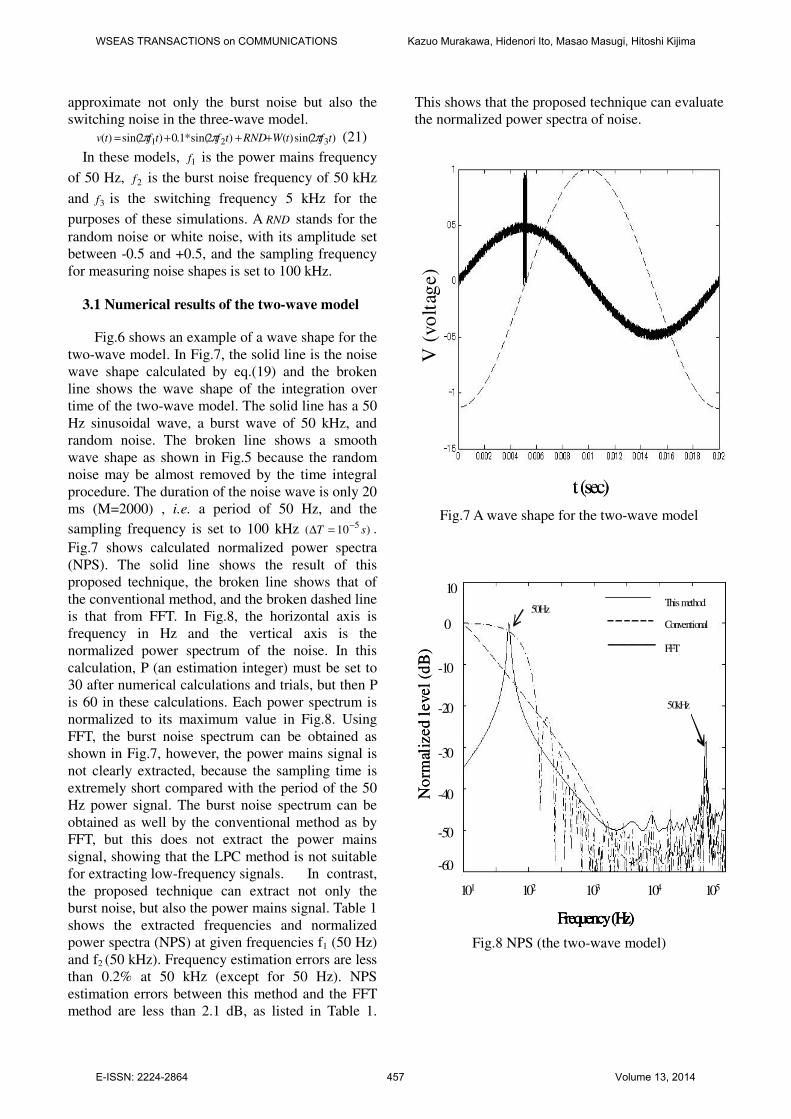
for measuring noise shapes is set to 100 kHz. 3.1 Numerical results of the two-wave model

Fig.6 shows an example of a wave shape for the

two-wave model. In Fig.7, the solid line is the noise

wave shape calculated by eq.(19) and the broken

line shows the wave shape of the integration over

time of the two-wave model. The solid line has a 50

Hz sinusoidal wave, a burst wave of 50 kHz, and

random noise. The broken line shows a smooth

wave shape as shown in Fig.5 because the random

noise may be almost removed by the time integral

procedure. The duration of the noise wave is only 20

ms (M=2000) , i.e. a period of 50 Hz, and the

sampling frequency is set to 100 kHz )10(5

sT−=∆ .

Fig.7 shows calculated normalized power spectra

(NPS). The solid line shows the result of this

proposed technique, the broken line shows that of

the conventional method, and the broken dashed line

is that from FFT. In Fig.8, the horizontal axis is

frequency in Hz and the vertical axis is the

normalized power spectrum of the noise. In this

calculation, P (an estimation integer) must be set to

30 after numerical calculations and trials, but then P

is 60 in these calculations. Each power spectrum is

normalized to its maximum value in Fig.8. Using

FFT, the burst noise spectrum can be obtained as

shown in Fig.7, however, the power mains signal is

not clearly extracted, because the sampling time is

extremely short compared with the period of the 50

Hz power signal. The burst noise spectrum can be

obtained as well by the conventional method as by

FFT, but this does not extract the power mains

signal, showing that the LPC method is not suitable

for extracting low-frequency signals. In contrast,

the proposed technique can extract not only the

burst noise, but also the power mains signal. Table 1

shows the extracted frequencies and normalized

power spectra (NPS) at given frequencies f1 (50 Hz)

and f2 (50 kHz). Frequency estimation errors are less

than 0.2% at 50 kHz (except for 50 Hz). NPS

estimation errors between this method and the FFT

method are less than 2.1 dB, as listed in Table 1.

This shows that the proposed technique can evaluate

the normalized power spectra of noise.

t (sec)

V (

vo

ltag

e)

t (sec)

V (

vo

ltag

e)

Fig.7 A wave shape for the two-wave model

102 104103 105102 104103 105

Frequency (Hz)

101

10

-10

-20

-30

-40

-50

0

-60

No

rmal

ized

level

(dB

)

This method

Conventional

FFT

50kHz

50Hz

102 104103 105102 104103 105

Frequency (Hz)

101 102 104103 105102 104103 105

Frequency (Hz)

101

10

-10

-20

-30

-40

-50

0

-60

No

rmal

ized

level

(dB

)

10

-10

-20

-30

-40

-50

0

-60

No

rmal

ized

level

(dB

)

This method

Conventional

FFT

50kHz

50Hz

Fig.8 NPS (the two-wave model)


E-ISSN: 2224-2864 457 Volume 13, 2014

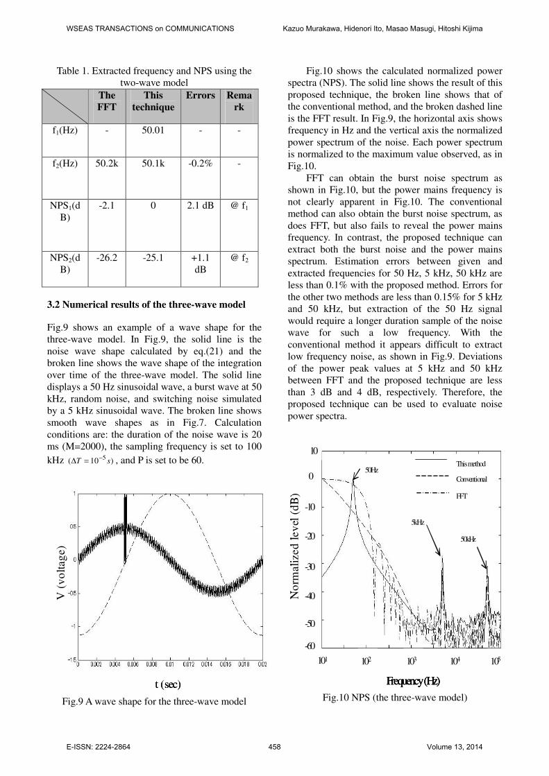
Table 1. Extracted frequency and NPS using the

two-wave model

The

FFT

This

technique

Errors Rema

rk

f1(Hz) - 50.01 - -

f2(Hz) 50.2k 50.1k -0.2% -

NPS1(d

B)

-2.1 0 2.1 dB @ f1

NPS2(d

B)

-26.2 -25.1 +1.1

dB

@ f2

3.2 Numerical results of the three-wave model

Fig.9 shows an example of a wave shape for the

three-wave model. In Fig.9, the solid line is the

noise wave shape calculated by eq.(21) and the

broken line shows the wave shape of the integration

over time of the three-wave model. The solid line

displays a 50 Hz sinusoidal wave, a burst wave at 50

kHz, random noise, and switching noise simulated

by a 5 kHz sinusoidal wave. The broken line shows

smooth wave shapes as in Fig.7. Calculation

conditions are: the duration of the noise wave is 20

ms (M=2000), the sampling frequency is set to 100

kHz )10(5

sT−=∆ , and P is set to be 60.

t (sec)

V (

vo

ltag

e)

t (sec)

V (

vo

ltag

e)

Fig.9 A wave shape for the three-wave model

Fig.10 shows the calculated normalized power

spectra (NPS). The solid line shows the result of this

proposed technique, the broken line shows that of

the conventional method, and the broken dashed line

is the FFT result. In Fig.9, the horizontal axis shows

frequency in Hz and the vertical axis the normalized

power spectrum of the noise. Each power spectrum

is normalized to the maximum value observed, as in

Fig.10.

FFT can obtain the burst noise spectrum as

shown in Fig.10, but the power mains frequency is

not clearly apparent in Fig.10. The conventional

method can also obtain the burst noise spectrum, as

does FFT, but also fails to reveal the power mains

frequency. In contrast, the proposed technique can

extract both the burst noise and the power mains

spectrum. Estimation errors between given and

extracted frequencies for 50 Hz, 5 kHz, 50 kHz are

less than 0.1% with the proposed method. Errors for

the other two methods are less than 0.15% for 5 kHz

and 50 kHz, but extraction of the 50 Hz signal

would require a longer duration sample of the noise

wave for such a low frequency. With the

conventional method it appears difficult to extract

low frequency noise, as shown in Fig.9. Deviations

of the power peak values at 5 kHz and 50 kHz

between FFT and the proposed technique are less

than 3 dB and 4 dB, respectively. Therefore, the

proposed technique can be used to evaluate noise

power spectra.

102 104103 105102 104103 105

Frequency (Hz)

10

-10

-20

-30

-40

-50

0

-60

No

rmali

zed

lev

el (

dB

)

101

This method

Conventional

FFT

5kHz

50kHz

50Hz

102 104103 105102 104103 105

Frequency (Hz)

10

-10

-20

-30

-40

-50

0

-60

No

rmali

zed

lev

el (

dB

)

101 102 104103 105102 104103 105

Frequency (Hz)

10

-10

-20

-30

-40

-50

0

-60

No

rmali

zed

lev

el (

dB

)

101

This method

Conventional

FFT

5kHz

50kHz

50Hz

Fig.10 NPS (the three-wave model)


E-ISSN: 2224-2864 458 Volume 13, 2014

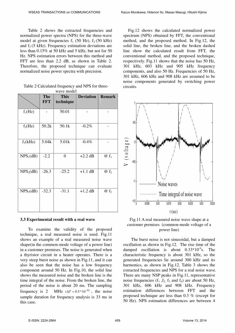
Table 2 shows the extracted frequencies and

normalized power spectra (NPS) for the three-wave

model at given frequencies f1 (50 Hz), f2 (50 kHz)

and f3 (5 kHz). Frequency estimation deviations are

less than 0.15% at 50 kHz and 5 kHz, but not for 50

Hz. NPS estimation errors between this method and

FFT are less than 2.2 dB, as shown in Table 2.

Therefore, the proposed technique can evaluate

normalized noise power spectra with precision.

Table 2 Calculated frequency and NPS for three-

wave model

The

FFT

This

technique

Deviation Remark

f1(Hz) - 50.01 - -

f2(Hz) 50.2k 50.1k -0.2% -

f3(kHz) 5.04k 5.01k -0.4% -

NPS1(dB) -2.2 0 +2.2 dB @ f1

NPS2(dB) -26.3 -25.2 +1.1 dB @ f2

NPS3(dB) -32.3 -31.1 +1.2 dB @ f3

3.3 Experimental result with a real wave

To examine the validity of the proposed

technique, a real measured noise is used. Fig.11

shows an example of a real measured noise wave

shape(in the common-mode voltage of a power line)

in a customer premises. The noise is generated when

a thyristor circuit in a heater operates. There is a

very steep burst noise as shown in Fig.11, and it can

also be seen that the noise has a low frequency

component around 50 Hz. In Fig.10, the solid line

shows the measured noise and the broken line is the

time integral of the noise. From the broken line, the

period of the noise is about 20 ms. The sampling

frequency is 2 MHz )610*5.0(

−=∆T , the noise

sample duration for frequency analysis is 33 ms in

this case.

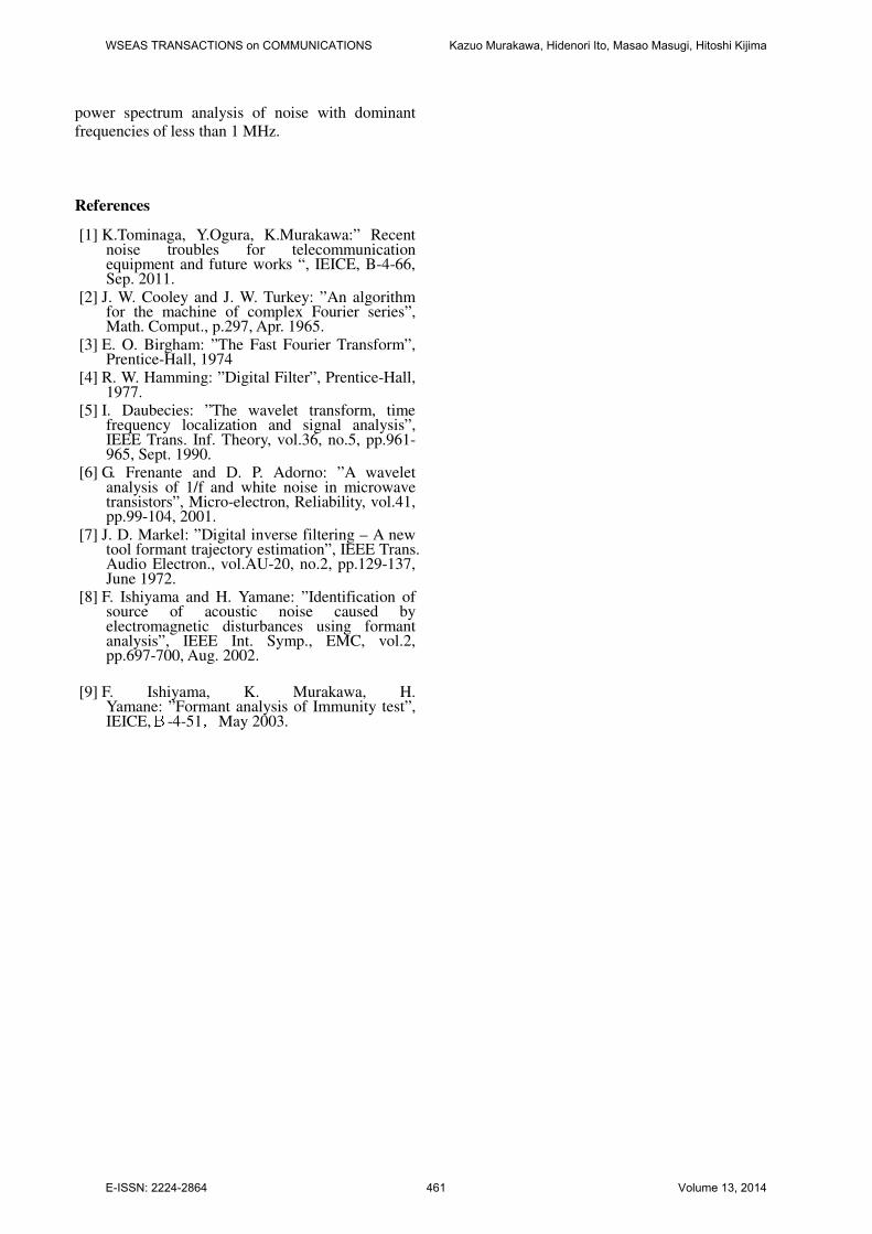
Fig.12 shows the calculated normalized power

spectrum (NPS) obtained by FFT, the conventional

method, and the proposed method. In Fig.12, the

solid line, the broken line, and the broken dashed

line show the calculated result from FFT, the

conventional method, and the proposed technique,

respectively. Fig.11 shows that the noise has 50 Hz,

301 kHz, 603 kHz and 905 kHz frequency

components, and also 50 Hz. Frequencies of 50 Hz,

301 kHz, 606 kHz and 908 kHz are assumed to be

noise components generated by switching power

circuits.

t (sec)

Noise waves

Time integral of noise wave

V (

vo

ltag

e)

t (sec)

Noise waves


t (sec)

Noise waves


V (

vo

ltag

e)

Fig.11 A real measured noise wave shape at a

customer premises (common-mode voltage of a

power line)

The burst noise is not sinusoidal, but a damped

oscillation as shown in Fig.12. The rise time of the

damped oscillation is about 0.33*10-6

s. The

characteristic frequency is about 301 kHz, so the

generated frequencies lie around 300 kHz and its

harmonics, as shown in Fig.12. Table 3 shows the

extracted frequencies and NPS for a real noise wave.

There are many NSP peaks in Fig.11, representative

noise frequencies (f1 ,f2, f3 and f4) are about 50 Hz,

301 kHz, 606 kHz and 908 kHz. Frequency

estimation differences between FFT and the

proposed technique are less than 0.3 % (except for

50 Hz). NPS estimation differences are between 4


E-ISSN: 2224-2864 459 Volume 13, 2014

dB and 10 dB (except for 50 Hz).

According to Fig.11, the damped oscillation peak

level is about 1.1, and the peak level of the power

mains frequency of 50 Hz is about 0.1 as shown in

Fig.10, with the estimated difference between FFT

and this technique at 50 Hz being -20.1dB

(=20log10(1.1/0.1)). This shows that FFT is likely to

overestimate the NPS level at 50 Hz, or extract a

wrong frequency in this case. If this conclusion is

correct, the estimated difference between FFT and

this technique at 50 Hz is 5 dB as shown inFig.12.

Numerical simulations show that the proposed

technique can extract dominant power spectrum

figures with high accuracy using a short-duration

time series.

Frequency (Hz)

No

rmal

ized

lev

el (

dB

)

102 104103 105101 106

This method

Conventional

FFT

f２f１ f３

f４Frequency (Hz)

No

rmal

ized

lev

el (

dB

)

102 104103 105101 106

This method

Conventional

FFT

Frequency (Hz)

No

rmal

ized

lev

el (

dB

)

102 104103 105101 106102 104103 105101 106

This method

Conventional

FFT

This method

Conventional

FFT

f２f１ f３

f４

Fig.12 NPS of a real noise

Table 3 Extracted frequency and NPS for a real

noise wave

The

FFT

This

technique

Deviation Remark

f1(Hz) 48.1 50.1 +4% -

f2(Hz) 302.1k 301.2k -0.3% -

f3(Hz) 604.2k 606.3k +0.3% -

f4(kHz) 907.2k 908.3k +0.1% -

NPS1(dB) 0.1

(-20.1)

-25.1 -25 dB

(-5 dB)

@ f1

NPS2(dB) -10 0 +10 dB @ f2

NPS3(dB) -13 -6 +7 dB @ f3

NPS4(dB) -30 -26 +4dB @ f4

4 Conclusions This paper shows that there are still serious

malfunctions of telecommunication equipment that

occur in the field, mainly due to noise from the

power circuits of electronic and electrical equipment.

This noise causes communication link interruption,

throughput reduction and sound quality degradation.

Most of the noise is below 150 kHz in this case. To

reduce the malfunctioning of telecommunication

equipment, it is important to extract noise power

spectra (frequencies and levels) to enable selection

of the most suitable noise filters to put on power

lines or telecommunication lines when it is

impractical to simply eliminate the source(s) of the

noise.

This paper also proposes a new technique based

on the conventional LPC method. The new

technique uses a time integral procedure on the

noise signal. The procedure is to minimize random

noise effects in frequency analysis, therefore, the

new technique can extract power spectra, and the

frequency extractions produced differ from

numerical simulations and actual measurements by

less than 4 %. The new technique can produce

normalized power spectra of noise without requiring

lengthy time series data, using shorter time series

than FFT requires in general.

Numerical results presented here show that the

proposed technique can be used for normalized


E-ISSN: 2224-2864 460 Volume 13, 2014

power spectrum analysis of noise with dominant

frequencies of less than 1 MHz.

References

[1] K.Tominaga, Y.Ogura, K.Murakawa:” Recent noise troubles for telecommunication equipment and future works “, IEICE, B-4-66, Sep. 2011.

[2] J. W. Cooley and J. W. Turkey: ”An algorithm for the machine of complex Fourier series”, Math. Comput., p.297, Apr. 1965.

[3] E. O. Birgham: ”The Fast Fourier Transform”, Prentice-Hall, 1974

[4] R. W. Hamming: ”Digital Filter”, Prentice-Hall, 1977.

[5] I. Daubecies: ”The wavelet transform, time frequency localization and signal analysis”, IEEE Trans. Inf. Theory, vol.36, no.5, pp.961-965, Sept. 1990.

[6] G. Frenante and D. P. Adorno: ”A wavelet analysis of 1/f and white noise in microwave transistors”, Micro-electron, Reliability, vol.41, pp.99-104, 2001.

[7] J. D. Markel: ”Digital inverse filtering – A new tool formant trajectory estimation”, IEEE Trans. Audio Electron., vol.AU-20, no.2, pp.129-137, June 1972.

[8] F. Ishiyama and H. Yamane: ”Identification of source of acoustic noise caused by electromagnetic disturbances using formant analysis”, IEEE Int. Symp., EMC, vol.2, pp.697-700, Aug. 2002.

[9] F. Ishiyama, K. Murakawa, H.

Yamane: ”Formant analysis of Immunity test”, IEICE,Ｂ-4-51，May 2003.


E-ISSN: 2224-2864 461 Volume 13, 2014

Normalized power spectrum analysis based on Linea ... · Normalized power spectrum analysis based...

Documents

Transcript of Normalized power spectrum analysis based on Linea ... · Normalized power spectrum analysis based...