Normalized ghost imaging

Normalized ghost imaging

Baoqing Sun,1,∗ Stephen S. Welsh,1 Matthew P. Edgar,1

Jeffrey H. Shapiro,2 and Miles J. Padgett1

1School of Physics and Astronomy, SUPA, University of Glasgow, G12 8QQ, UK2Research Laboratory of Electronics, Massachusetts Institute of Technology, Cambridge,

Massachusetts 02139, USA∗[email protected]

www.gla.ac.uk/schools/physics/research/groups/optics/

Abstract: We present an experimental comparison between differentiterative ghost imaging algorithms. Our experimental setup utilizes a spatiallight modulator for generating known random light fields to illuminate apartially-transmissive object. We adapt the weighting factor used in thetraditional ghost imaging algorithm to account for changes in the efficiencyof the generated light field. We show that our normalized weightingalgorithm can match the performance of differential ghost imaging.

© 2012 Optical Society of America

OCIS codes: (030.4280) Noise in imaging systems; (030.6140) Speckle; (110.1650) Coher-ence imaging; (200.1130) Algebraic optical processing.

References and links1. R. S. Bennink, S. J. Bentley, and R. W. Boyd, “‘Two-photon’ coincidence imaging with a classical source,” Phys.

Rev. Lett. 89, 113601 (2002).2. A. Gatti, E. Brambilla, M. Bache, and L. A. Lugiato, “Ghost imaging with thermal light: Comparing entangle-

ment and classical correlation,” Phys. Rev. Lett. 93, 093602 (2004).3. A. Gatti, E. Brambilla, M. Bache, and L. A. Lugiato, “Correlated imaging, quantum and classical,” Phys. Rev. A

70, 013802 (2004).4. A. Valencia, G. Scarcelli, M. D’Angelo, and Y. Shih, “Two-photon imaging with thermal light,” Phys. Rev. Lett.

94, 063601 (2005).5. F. Ferri, D. Magatti, A. Gatti, M. Bache, E. Brambilla, and L. A. Lugiato, “High-resolution ghost image and

ghost diffraction experiments with thermal light,” Phys. Rev. Lett. 94, 183602 (2005).6. J. H. Shapiro, “Computational ghost imaging,” Phys. Rev. A 78, 061802 (2008).7. Y. Bromberg, O. Katz, and Y. Silberberg, “Ghost imaging with a single detector,” Phys. Rev. A 79, 053840

(2009).8. M. Duarte, M. Davenport, D. Takhar, J. Laska, T. Sun, K. Kelly, and R. Baraniuk, “Single-pixel imaging via

compressive sampling,” IEEE Signal Processing Magazine 25, 83–91 (2008).9. F. Ferri, D. Magatti, L. A. Lugiato, and A. Gatti, “Differential ghost imaging,” Phys. Rev. Lett. 104, 253603

(2010).10. J. Goodman, Statistical Optics (Wiley, 2000).11. S. Boyd and L. Vandenberghe, Convex Optimization (Cambridge University Press, 2004).12. D. L. Donoho and Y. Tsaig, “Fast solution of l1-norm minimization problems when the solution may be sparse,”

IEEE Trans. Inf. Theory 54, 4789–4812 (2008).13. O. Katz, Y. Bromberg, and Y. Silberberg, “Compressive ghost imaging,” Appl. Phys. Lett. 95(13), 131110 (2009).

1. Introduction

Classical ghost imaging (GI) [1–5] uses a series of random light patterns to illuminate an un-known object. For each pattern the reflected or transmitted light is measured using a single

#165380 - $15.00 USD Received 23 Mar 2012; revised 14 May 2012; accepted 27 Jun 2012; published 11 Jul 2012(C) 2012 OSA 16 July 2012 / Vol. 20, No. 15 / OPTICS EXPRESS 16892

element detector. The series of single element measurements, combined with the known lightpatterns is used to deduce the object. In some systems the random light pattern is produced asa time varying laser speckle, and a beam splitter is used to illuminate both the unknown objectand a reference camera, with which the pattern is recorded. Subsequently, the need for the beamsplitter and camera has been removed by implementing a spatial light modulator (SLM) to pro-duce a random, but known, pattern thereby reducing the number of components in the systemnecessary for GI experiments [6, 7]. This latter approach is known as computational GI and interms of the experimental arrangement is closely related to the field of single pixel cameras [8].

In all approaches to GI an algorithm is employed to deduce the object using the series ofmeasurements from the single element detector and either the recorded or computationallypredicted random patterns. The algorithms employed fall into two categories, iterative onesthat give a refined estimate of the object after every new light pattern and measurement, andinversion ones which infer an object based on the entire series of patterns and measurements.

Iterative algorithms use the measured signal to derive a weighting factor to the correspond-ing pattern that is then added to the iterative estimate of the object. In this paper we comparea number of these iterative algorithms within the context of computational GI. The algorithmswe consider are traditional GI (TGI) and differential GI (DGI) [9]. In a computational GI setup,TGI uses a weighting factor equal to the signal from the detector whereas DGI utilizes a weight-ing factor that depends on fluctuations in the measured signal and uses an additional detector togive a normalization. Beyond these two algorithms we introduce a variant of the TGI algorithm,normalized GI (NGI), which we show can match the performance of DGI.

Key to all these algorithms is that the changes in the measured signal should arise from theoverlap of the known random pattern with the unknown object. Obviously other sources ofsignal change are possible; including fluctuations arising from changes in the source intensityand changes in the efficiency with which the pattern is imprinted. These later sources of noisescale with the signal level and hence become more significant when the signal is high.

2. Experimental setup

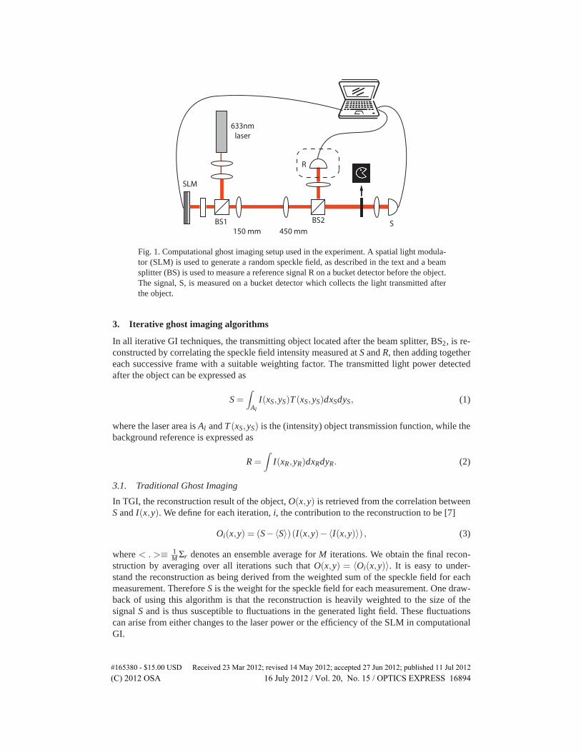
The experimental setup is shown in Fig. 1. Here a random light pattern is generated from asimulated superposition of plane waves using random numbers, which is then sent to an SLMto produce a synthesized speckle field. The SLM has 512× 512 pixels in the window of size3.584×3.584mm. We pass a collimated laser of wavelength λ = 632.8nm through a polarizingbeam splitter and a half-wave plate, before illuminating the SLM window. The speckle field isgenerated by modulation of the SLM and the returning light field is then magnified by a simpletelescope system consisting of 150mm and 450mm biconvex lenses. The object is located atthe focus plane of the 450mm lens, which is also the image plane of the SLM window. A 50 : 50beam splitter is placed before the object in order to split the speckle field into two beams; theobject beam (I(xS)) and the reference beam (I(xR)). The object beam illuminates the object andis then collected by a bucket detector, thus providing an computational GI setup. The additionalreference beam for monitoring the light differentiates our system from previous experimentalcomputational GI configurations. Since we are generating a computer hologram that is then sentto the SLM to create the speckle field, we can therefore predict the light field at the referencearm, negating the demand for a CCD camera, and requiring only a second bucket detector.It should be noted that for TGI based on our computational GI setup, only the object bucketdetector is needed. The additional bucket detector in the reference arm is only required for NGIand DGI. Light intensities detected by the object and reference bucket detectors are indicatedby S and R respectively, and the speckle field is described by I(x,y). As we use a 50 : 50 beamsplitter, it is understood that I(x,y) = 2I(xS,yS) = 2I(xR,yR).


633nmlaser

SLM

450 mm150 mmBS1 BS2 S

R

Fig. 1. Computational ghost imaging setup used in the experiment. A spatial light modula-tor (SLM) is used to generate a random speckle field, as described in the text and a beamsplitter (BS) is used to measure a reference signal R on a bucket detector before the object.The signal, S, is measured on a bucket detector which collects the light transmitted afterthe object.

3. Iterative ghost imaging algorithms

In all iterative GI techniques, the transmitting object located after the beam splitter, BS2, is re-constructed by correlating the speckle field intensity measured at S and R, then adding togethereach successive frame with a suitable weighting factor. The transmitted light power detectedafter the object can be expressed as

S =

∫Al

I(xS,yS)T (xS,yS)dxSdyS, (1)

where the laser area is Al and T (xS,yS) is the (intensity) object transmission function, while thebackground reference is expressed as

R =

∫I(xR,yR)dxRdyR. (2)

3.1. Traditional Ghost Imaging

In TGI, the reconstruction result of the object, O(x,y) is retrieved from the correlation betweenS and I(x,y). We define for each iteration, i, the contribution to the reconstruction to be [7]

Oi(x,y) = (S−〈S〉)(I(x,y)−〈I(x,y)〉) , (3)

where < . >≡ 1M Σr denotes an ensemble average for M iterations. We obtain the final recon-

struction by averaging over all iterations such that O(x,y) = 〈Oi(x,y)〉. It is easy to under-stand the reconstruction as being derived from the weighted sum of the speckle field for eachmeasurement. Therefore S is the weight for the speckle field for each measurement. One draw-back of using this algorithm is that the reconstruction is heavily weighted to the size of thesignal S and is thus susceptible to fluctuations in the generated light field. These fluctuationscan arise from either changes to the laser power or the efficiency of the SLM in computationalGI.


3.2. Differential ghost imaging

Differential GI [9], first performed by Ferri et al, utilizes a second bucket detector to extracta reference signal which is used in the reconstruction to weight the speckle field based on theaverage transmission signal relative to the average reference signal. Similarly, each contributionto the reconstruction can be expressed as

Oi(x,y) =

(S− 〈S〉

〈R〉R

)(I(x,y)−〈I(x,y)〉) . (4)

Thus we obtain the final result by summing for all iterations. We observe the second term inbrackets on the right hand side of Eq. (3) and Eq. (4) are both identical however the first termin brackets of Eq. (4) is now weighted according to the average value of S, which is normalizedto the average value of R. As demonstrated in [9] the DGI algorithm improves by order ofmagnitude the SNR of the measurement with respect to TGI. Moreover, a key difference fromTGI, it is no longer sensitive to other sources of noise. For example, fluctuations in the laserpower or changes to the SLM efficiency will affect both the reference signal and the transmittedsignal, and thus the contribution to the reconstruction will be weighted more appropriately.

3.3. Normalized ghost imaging

3.3.1. Normalized ghost imaging with two detectors

As seen in Eq. (4), larger values of S measured by the bucket detector results in a greater weightfor that particular speckle field, therefore external noise sources can still affect the overall re-construction. There exists another iterative algorithm which instead normalizes each individualmeasurement S, as well as the running average, according to the reference signal R, resultingin an arguably more intuitive approach for dealing with time varying noise sources. We callthis approach normailized GI (NGI). The algorithm used to describe each contribution to thereconstruction in NGI is given by

Oi(x,y) =

(SR− 〈S〉

〈R〉)(I(x,y)−〈I(x,y)〉) , (5)

where we have assumed 〈S〉〈R〉 ≈

⟨SR

⟩for a large number of measurements. By considering Eqs.

(4) and (5) we can summarize the difference between the two algorithms as

〈O(x,y)NGI〉= 1〈R〉〈O(x,y)DGI〉 . (6)

3.3.2. Normalized ghost imaging with a single detector

In a computational GI setup, we can show that the additional detector used to measure the ref-erence signal in DGI and NGI can instead be estimated based on the known light field reflectedfrom the SLM and the average measured signal S for an arbitrary number of previous iterations.Calculating R negates the requirement for an additional detector, whilst improving the perfor-mance of the reconstruction compared to TGI, thus single-detector NGI (SNGI) is identical tothe TGI experimental setup, with only a modified algorithm.

3.4. Signal-to-noise ratio analysis

To make a quantitative comparison between the NGI and the existing algorithms, we adopta similar approach as used by Ferri et al and investigate the theoretical contribution to thesignal-to-noise ratio (SNR) for objects with varying transmission functions. In [9] the authors


(a) (b)

Fig. 2. (a) A typical speckle pattern hologram. (b) The measured intensity distribution ofthe speckle pattern (blue) and an exponential curve (red).

express the average quantity of Eq. (4) in terms of the object transmission fluctuation δT (x,y)=T (x,y)−T ,

〈O(x,y)DGI〉= As 〈I〉2 δT (x,y), (7)

where As is the average speckle area and T =∫

Al〈I(x,y)〉T (x,y)dxdy/

∫Al〈I(x,y)〉dxdy is the

average transmission function of the object. Note that Eq. (7) is obtained under the assump-tions of uniform illumination (the average speckle beams are constant over their area) andperfect resolution (the speckle area is much smaller compared to features of the object). Thecorresponding signal of DGI can be defined as

(Δ〈ODGI〉)2 = As2 〈I〉4 (ΔT )2, (8)

where ΔT is the variation of the object transmission function to be detected. Similarly, usingEq. (6), we can express the signal of NGI as

(Δ〈ONGI〉)2 = As2 〈I〉4

〈R〉2 (ΔT )2. (9)

The speckle patterns used in our experiment exhibit complex-Gaussian behaviour, such thatthe intensity is exponentially distributed (see Fig. 2), and the noise associated to the measure-ment of O(x,y) can be expressed as

⟨δO2(x,y)

⟩=⟨O(x,y)2⟩−〈O(x,y)〉2 , (10)

for which it can be shown that 〈O(x,y)〉= 0, thus the second term on the right hand side (RHS)of in Eq. (10) may be omitted. Again, under the assumptions of uniform illumination and perfectresolution, the noise of DGI can be expressed as

⟨O2

DGI

⟩≈ AsAl 〈I〉4 δT 2, (11)

where δT 2 = T 2−T2

and T 2 =∫

Al〈I(x,y)〉T 2(x,y)dxdy/

∫Al〈I(x,y)〉dxdy. Using linearization

we can writeSR≈ 〈S〉

〈R〉(

1+δS〈S〉 −

δR〈R〉

), (12)


where δS and δR are the zero-mean deviation of S and R, thus the noise of NGI is shown to be

⟨O2

NGI

⟩≈ AsAl〈I〉4

〈R〉2 δT 2. (13)

Finally, we show that the SNR contribution for NGI is

SNRNGI = SNRDGI =M

Nspeckle

ΔT 2

δT 2, (14)

where Ns = Al/As is the number of speckles in the field. The SNR contribution for NGI is foundto be identical to that of the DGI algorithm derived in [9]. For comparison the SNR contributionfor TGI was shown to be

SNRTGI =M

Nspeckle

ΔT 2

T 2. (15)

Therefore we can examine the difference between the NGI (or DGI) and TGI algorithms byobtaining the ratio of SNR calculations, given as

SNRNGI

SNRTGI= 1+

T2

T 2 −T2 . (16)

As highlighted by Ferri et al, the difference is always greater than 1 and dependent only uponthe variation in the object transmission function.

4. Experiment results

We generated a series of random speckle patterns using an SLM by simulating the interferenceof many plane waves on a computer. The real and imaginary amplitude components and thewave vector �k of each simulated plane wave is Gaussian distributed. Figure 2 shows a typi-cal example of the speckle patterns generated on the SLM and the exponentially distributedintensity for many patterns, implying that the speckle hologram has complex-Gaussian statis-tics, thereby a good approximation for real speckle fields [10]. A binary transmissive object,5mm× 5mm in size, is located after a 3× magnification telescope in the image plane of theSLM. Since we know both the object and the random speckle field projected to the SLM, weare able to simulate the expected results for comparison with our experiment. Experimental andsimulated reconstruction results after 10000 iterations are shown in Fig. 3. The simulated re-construction is produced assuming no external noise sources. The partially transmissive objectused is indicated in the bottom right of Fig. 3. It is clear that the DGI and NGI algorithmsprovide very similar results, as predicted from the theory, and both show improved backgroundsubtraction compared to TGI.

Compared with the traditional computational GI setup, the NGI algorithm requires a refer-ence bucket detector. However, as discussed in section 3.3.2, the advantage of computationalGI means that we can replace this bucket detector with a virtual reference detector generatinga simulated R. Thus we can negate the requirement for the reference detector and return thesystem to a true single element camera, which we call single-detector NGI (SNGI). The twomajor factors that dominate the value of R are from the different speckle patterns displayed onthe SLM and fluctuations of the incident laser power. We can computationally predict changesto the value of R due to the speckle pattern, whereas fluctuations of the laser power can be sim-ulated by using a rolling average for a particular series of S measurements. The bottom row inFig. 3 shows the experimental results for reconstructing the object using the SNGI algorithm.


iterations

TGI

DGI

NGI

SNGI

simulationexperimentalgorithm

object10000100010010

Fig. 3. Experimental results (middle column) for TGI, DGI and NGI reconstruction algo-rithms as they evolve (10, 100, 1000 and 10000 iterations from left to right, respectively)with the corresponding simulated results (right column). The transmissive object is shownin the lower right. The bottom row shows the evolution for reconstructing the object withthe NGI algorithm using a single detector and predicting the reference signal R, termedhere the SNGI algorithm.

We observe similar results compared with DGI and NGI algorithms indicating an improvedperformance compared with the TGI algorithm for single element camera.

To demonstrate the effect of object transmission function on the performance of NGI com-pared with TGI and DGI algorithms we used a similar experimental approach to that in Ref. [9].By scanning a knife edge (located in the image plane of the SLM, as before) across the specklefield in well defined steps (for which ΔT = 1), we measured the SNR’s for the final object recon-struction obtained after 5000 random speckle iterations. The beam size used was 10× 10mmand the speckle size at the plane of the object was found to be δs ∼ 90 μm, providing aroundNs ∼ 12500 speckles. The experimental results and theoretical predictions for the SNR’s of eachiterative algorithm are shown in Fig. 4. Note that the y-axis has been normalized to the numberof iterations. We observe close quantitative agreement between the theory and the measure-ments. The results indicate that for low transmissive objects, all algorithms reconstruct withsimilar SNR, while for more transmissive objects the DGI and NGI algorithms become moreefficient in comparison to TGI due to the differential nature of the reconstruction. Further-more, we observe that when using a single detector, SNGI is a more efficient algorithm forreconstructing objects of all transmissions compared to TGI. We observe that for increasingtransmissive objects SNGI becomes less efficient than NGI, for which the reason is the subjectof ongoing research. Similar to [9], we find a systematic discrepancy between the experimentalresults of TGI and the theoretical predictions.


Fig. 4. Signal-to-noise ratio’s for DGI, NGI, SNGI and TGI versus transmitting area. Trans-mitting ratio is defined as the ratio between the transmitting area of the object and the areaof the speckle field.

5. Normalization in matrix inverse algorithms

5.1. Introduction to matrix inverse algorithms and compressive sensing

As an alternative to the iterative techniques discussed above, we can choose to record all thesignals for a complete set of speckle patterns and then treat the image reconstruction as one ofmatrix inversion. The series of M speckle patterns, each containing N pixels can be representedby a M ×N matrix. If the object is also represented as an N element column vector, then thevector containing the measured signals is a M element vector. This relationship is expressed as

⎡⎢⎣

Si...

SN

⎤⎥⎦=

⎡⎣ M×N

⎤⎦×

⎡⎣ T(x,y)

⎤⎦ . (17)

In the case where the number of speckle patterns equals the number of pixels then the M×Nmatrix is square, such that its inverse can be calculated and the object vector determined. How-ever when M < N and or N is large, the system is ill-conditioned and calculating the inverseof the matrix is not straightforward. Problems of this type are wide spread in physics and tech-niques for solving them have been developed. Within our system the appeal is to reconstruct theimage of N pixels from M measurements where M <N. That this is possible is based on the factthat natural images are sparse and the reconstruction can be obtained by solving a convex opti-mization problem [11], which is a generalization of a linear least squares problem. In contrastto iterative methods, compressive GI (CGI) needs to take all measurements, represented here,in some compressible basis (in this case a discrete cosine transform which has been applied toeach row of the M×N matrix). Solving the convex optimization problem requires minimizingthe �1 norm [12].


Fig. 5. (a) Experimental result of Normalized known vector reconstruction method (S/R)having SNR = 9.95. (b) Standard CGI reconstruction from S having SNR = 7.39.

5.2. Normalized compressive ghost imaging

By normalizing the measured object signal relative to the reference signal as performed above,such that S′ ≡ S/R, we can apply the CGI technique [13] to reconstruct our object. Equation (17)can then be written for normalized CGI (NCGI) as⎡

⎢⎣S′i...

S′N

⎤⎥⎦=

⎡⎣ M×N

⎤⎦×

⎡⎣ T(x,y)

⎤⎦ . (18)

Performing both NCGI and CGI analyses using the same experimental data (acquired usingthe experimental setup in Fig. 1) we obtain the reconstruction in Fig. 5. We observe a clear im-provement using the NCGI algorithm compared to the CGI algorithm, manifest as an increasedSNR value. The efficiency with which NCGI can reconstruct sparse images over CGI is deter-mined by the level of noise in the system. We find that when there is no system noise present,both reconstructions are essentially identical. Thus the main improvement in employing NCGIover CGI with the additional reference detector is the ability to protect the reconstruction fromtime varying noise sources.

6. Conclusion

In conclusion we have compared different iterative GI methods to reconstruct an object andstudied a new GI algorithm, which we call normalized GI (NGI). The performance of the dif-ferential GI (DGI) and NGI algorithms show good quantitative agreement as predicted by thetheoretical foundations that support them. Our results indicate that by normalizing the meas-ured signal relative to a reference signal, a more appropriate weighting factor is applied to theensemble average of the estimated object, compared to the traditional GI (TGI) algorithm. Ouranalysis of the measured SNR and the object transmission shows a significant improvement formore transmissive objects in comparison to TGI. Furthermore, we have shown it is possible toapply normalization to systems with a single detector, SNGI, by estimating the reference signal.We have also investigated normalization within a compressive matrix inversion method, show-ing similar results to an non-normalized algorithm but with enhanced noise suppression. Webelieve the NGI algorithm will be a useful resource for imaging where alternative techniquesare required in the future.


Acknowledgments

At the time when this work was ready for publication the authors found through private com-munication with Alessandra Gatti and Fabio Ferri that they had similar findings, for whomwe thank for useful discussion. MJP would like to thank the Royal Society and the WolfsonFoundation. The work of JHS was supported by the DARPA Information in a Photon (InPho)Program. We gratefully acknowledge the financial support from the UK EPSRC.


Normalized ghost imaging

Documents

Transcript of Normalized ghost imaging