NONPOINT SOURCE POLLUTION

G W LF

GENERALIZED WATERSHED LOADING FUNCTIONS

VERSION 2.0

USER'S MANUAL

December 15, 1992

Douglas A. Haith, Ross Mandel & Ray Shyan Wu

PRECIPITATIOH

(Rain, Snow Melt, ~~~igation)

.,.,.--

-------~~-

RUNOFF

NONPOINT SOURCE POLLUTION

Department of Agricultural & Biological Engineering Cornell University RDey-Robb Hall

Ithaca NY USA 14853

TABLE OF CONTENTS

INTRODUCTION ....................................................................................................................................... 1

MODEL DESCRIPTION ............................................................................................................................ 2

Model Structure ............................................................................................................................... 2 Input Data......................................................................................................................................... 2 Model Output ...............................................................................................................•...................• 3

GWLF PROGRAM .....•.........•...•....................•...................•.•............•.................•.•........••.......•.•...•..........•.. 3

Required FOes .....•..•.....•......•..•....••.•................•.....................•......••••.•....................•...•.........••........... 3 Program Structure ..•.•.•••..•......••.••..............•....•............•.......•.....••••....••...............•.••.........•................ 4 Transport Data Manipulation........................................................................................................... 4 Nutrient Data Manipulation .........•.....•..............•............................................................................... 5

Simulation ··········~······························································································································ 5 Results Output ...••.....••.•••..••....•....••....•.....•....••.....•••...........•...............................................•.............. 6

EXAMPLE 1: 4-YEAR STUDY IN WEST BRANCH DELAWARE BASIN ................................................ 7

Simulation ....•.......••.........•.....•...••....•.........................•.............••••......•.•.••..........••...............••......•••.... 7 Results Generation ...........•.•....•.....••...............•..••.......••...•....•....................•......................•...••.........• 8

EXAMPLE 2: EFFECTS OF EUMINATION OF WINTER MANURE SPREADING ................................ 8

Nutrient Parameters Modification ..•.........•............•........ :................................................................. 8 Simulation and Results Generation ...•...•.••...•........................••..........•.•.•..................•.•.................... 1 o

EXAMPLE 3: A 30-YEAR SIMULATION STUDY..................................................................................... 12

APPENDIX A: MATHEMATICAL DESCRIPTION OF GWLF ........................................•................•......... 15

General Structure ............................................................................................................................. 15 Rural Runoff Loads ...................................•................•......................•.......•...................................... 15 Urban Runoff ....••....•.••....•........•..•.....................................••....•.......•..............•................•................. 18 Groundwater Sources····················································································-···;............................ 19 Septic (On-site Wastewater Disposal) Systems ....................................... ::.................................... 21

APPENDIX B: DATA SOURCES & PARAMETER ESTIMATION ............................................................ 23

Land Use Data .•........••.•...•......•..•................•.....••••.....•....•....•.................•......................•....•.............. 23 Weather Data ••.•.•••..••.............••..•............•...•......•.•..............................•.............................•............... 23 Transport Parameters ..•.....•.....••..........................•...•....•.............•••••••.....•.•.......•...•....•........••••.••...... 23 Nutrient Parameters .....••...•.•...........•...•.........•.........•.•...............•.•....... ................ ......•............•.••...... 37

APPENDIX C: VAUDATION STUDY ........................................................................................................ 42

Water Quality Observations .••••.•......•....•..........••.•..............•••...•.......•...•.......................•...••......•......• 42 Watershed Data •.•••.•••.•.•.•....••••..•......•......••........••......•...•..••.••.•...•..•....•......•............•..........•.............. 43 Validation Results............................................................................................................................. 47 Conclusions .•..•••.••••••••..••••...••.•.••.....•..•............•.•.........................•.•.•.•....•..•...............•••................•... 49

APPENDIX D: DATA AND OUTPUT USTINGS FOR VAUDATON STUDY (EXAMPLE 1) ........•.......... 51

REFERENCES ......•..•................•.....••.••.........................••.....••......................................•....••..........•.....••.... 60

INTRODUCTION

Mathematical models for estimating nonpoint sources of nitrogen and phosphorus in streamflow indude export coefficients, loading functions and chemical simulation models. Export coefficients are average annual unit area nutrient loads associated with watershed land uses. Coefficients provide gross estimates of nutrient loads, but are of limited value for determining seasonal loads or evaluating water pollution control measures. Chemical simulation models are mechanistic (mass balance) descriptions of nutrient availability, wash off, transport and losses. Chemical simulation models provide the most complete descriptions of nutrient loads, but they are too data intensive for use in many water quality studies.

Loading functions are engineering compromises between the empiricism of export coefficients and the complexity of chemical simulation models. Mechanistic modeling is limited to water and/or sediment movement. Chemical behavior of nutrients is either ignored or described by simple empirical relationships. Loading functions provide useful means of estimating nutrient loads when chemical simulation models are impractical.

The Generalized Watershed Loading Functions (GWLF) model described In this manual estimates dissolved and total monthly nitrogen and phosphorus loads in streamflow from complex watersheds. Both surface runoff and groundwater sources are included, as well as nutrient loads from point sources and onsite wastewater disposal (septic) systems. In addition, the model provides monthly streamflow, soil erosion and sediment yield values. The model does not require water quality data for calibration, and has been validated for an 85,000 ha watershed in upstate New York.

The model described In this manual is a based on the original GWLF model as described by Haith & Shoemaker (1987). However, the current version (Version 2.0) contains several enhancements. Nutrient loads from septic systems are now included and the urban runoff model has been modified to more closely approximate procedures used in the Soil Conservation Service's Technical Release 55 (Soil Conservation Service, 1986) and models such as SWMM (Huber & Dickinson, 1988) and STORM (Hydrologic Engineering Center, 1977). The groundwater model has been given a somewhat stronger conceptual basis by limiting the unsaturated zone moisture storage capacity. The graphics outputs have been converted to VGA and color has been used more extensively.

The most significant changes in the manual are an expanded mathematical description of the model (Appendix A) and much more detaUed guidance on parameter estimation (Appendix B). Both changes are in response to suggestions by many users. The extra mathematical details are for the benefit of researchers who wish to modify (and improve) GWLF for their own purposes. The new sections on parameter estimatior (and the many new tables) are for users who may not be familiar with curve numbers, erosivity coefficients. etc., or who do not have access to some of the primary sources. The general intent has been to make the manual self-contained.

This manual describes the computer software package which can be used to implement GWLF. Thr associated programs are written in QuickBASIC 4.5 for personal computers using the MS-DOS operatinr system and VGA graphics. The manual and associated programs (on floppy disk) are available withou charge from the senior author. The programs are distributed in both executable (.EXE) and source codf form (.BAS). Associated example data files and outputs for Example 1 and a 30-yr weather set for Walter NY used in Example 3 are also included on the disk.

The main body of this manual describes the program structures and input and output files and option~ Three examples are also presented. Four appendices present the mathematical structure of GWLF, method: for estimation of model parameters, results of a validation study, and sample listings of input and output file~

In this manual, the program name, options in the menu page, and input by the user are written in bolo underline and italic, respectively.

MODEL DESCRIPTION

Model Structure

The GWLF model includes dissolved and solid-phase nitrogen and phosphorus in streamflow from the sources shown in Figure 1. Rural nutrient loads are transported In runoff water and eroded soil from numerous source areas, each of which is considered uniform with respect to soil and cover. Dissolved loads from each source area are obtained by multiplying runoff by dissolved concentra-tions. Runoff Is computed by using the Soil Conservation Service Curve Number Equation. Solid-phase rural nutrient loads are given by the product of monthly sediment yield and average sediment nutrient concentrations. Erosion is computed using the Universal Soil Loss Equation and the sediment yield Is the product of erosion and sediment delivery ratio. The yield in any month Is proportional to the total transport capacity of daily runoff during the month. Urban nutrient loads, assumed to be entirely solid-phase, are modeled by exponential accu- Figure 1. Nutrient Sources in GWLF. mulation and washoff func-

Rura~

Urban Runo-Ff"

tions. Septic systems are classified according to four types: normal systems, ponding systems, shortcircuiting systems, and direct discharge systems. Nutrient loads from septic systems are calculated by estimating the per capita daily load from each type of system and the number of people in the watershed served by each type. Daily evapotranspiration is given by the product of a cover factor and potential evapotranspiration. The latter is estimated as a function of daylight hours, saturated water vapor pressure and daily temperature.

Streamflow consists of runoff and discharge from groundwater. The latter is obtained from a lumped parameter watershed water balance. Daily water balances are calculated for unsaturated and shallow saturated zones. lnfUtration to the unsaturated and shallow saturated zones equals the excess, If any, of rainfall and snowmelt less runoff and evapotranspiration. Percolation occurs when unsaturated zone water exceeds field capacity. The shallow saturated zone is modeled as a linear groundwater reservoir.

Model structure, including mathematics, is discussed In more detail In Appendix A.

Input Data

The GWLF model requires daily precipitation and temperature data, runoff sources and transport a~ chemical parameters. Transport parameters include areas, runoff curve numbers for antecedent moisture condition II and the erosion product K•LS•C•P for each runoff source. Required watershed transport arameters· are groundwater recession and seepage coeffacaents, the available water capacity of th~

unsaturat zone. t e s amen e e ~110 a mont ly values for evapotranspiration cover tactqrs, . average daylight hours, growang season anleators and rainfall erosivity coefficients. Initial values must also oe specmea tot unsaturated arid shallow saturated zones, snow cover and 5-day antecedent rain fall plus

2

snowmelt.

Input nutrient data for rural source areas are dissolved nitrogen and phosphorus concentrations in runoff and solid-phase nutrient concentrations in sediment. If manure is spread during winter months on any rural area, dissolved concentrations in runoff are also specified for each manured area. Daily nutrient accumulation rates are required for each urban land use. Septic systems need estimates of the per capita nutrient load in septic system effluent and per capita nutrient losses due to plant uptake, as well as the number of people served by each type of system. Point sources of nitrogen and phosphorus are assumed to be in dissolved form and must be specified for each month. The remaining nutrient data are dissolved nitrogen and phosphorus concentrations in groundwater.

Procedures for estimating transport and nutrient parameters are described In Appendix B. Examples are given in Appendix C and in subsequent sections of this manual.

Model Output

The GWLF program provides its simulation results in tables as well as in graphs. The following principal variables are given:

Monthly Streamflow Monthly Watershed Erosion and Sediment Yield Monthly Total Nitrogen and Phosphorus Loads in Streamflow Annual Erosion from Each Land Use Annual Nitrogen and Phosphorus Loads from Each Land Use

The program also provides

Monthly Precipitation and Evapotranspiration Monthly Ground Water Discharge to Streamflow Monthly Watershed Runoff Monthly Dissolved Nitrogen and Phosphorus Loads in Streamflow Annual Dissolved Nitrogen and Phosphorus Loads from Each Land Use Annual Dissolved Nitrogen and Phosphorus Loads from Septic Systems

GWLF PROGRAM

Required Files

Simulations by GWLF require four program modules and three data files on the default drive. The three necessary data files are WEATHER.DAT, TRANSPRT.DAT and NUTRIENT.DAT. The four compiled modules, GWLF20.EXE, TRAN20.EXE, NUTR20.EXE, and OUTP20.EXE are run by typing GWLF20.

Two daily weather files for Walton, NY are included on the disks. WALT478.382 Is the four year (4/78-3/92) record used for model validation and in Examples 1 and 2. WALT462.392 is the 30 year (4/62- 3/92) record used in Example 3. Prior to running the programs, the appropriate weather record should be copied to WEATHER.DAT.

The final two data files on the disks (RESULTS.DAT, and SUMMARY.DAT) are output files from Example 1. GWLF20.BAS, TRAN20.BAS, NUTR20.BAS, and OUTP20.BAS are the uncompiled, OulckBASIC files for the modules, and can be used to modify the existing program.

3

', ···:,~ '; .

Program Structure

The structure of GWLF is illustrated in Figure 2. Once the program has been activated, the main control page appears on the screen, as shown in OISPLA Y 1. This page is the main menu page that leads to the four major options of the program. The selection of a program option provides access to another set of menu pages within the chosen option. After completing an option, the program returns the user to the main menu page for further actions.

The selection of the menu options is done by typing the number indicating a choice and then Enter.

Select one of the following : .·. . . i) . .. · ... 1 . Create or print TRANSPRT:DAT. (Transport parameters) 2 >create. or print NUTRIENT~DAT (n~trient parameters)

?

3 4 5

(TRANSPRT.DAT.must be. created beforeNUTRIENT.DAT) Run simulation · Obtain output Stop (End)

DISPLAY 1. The Main Menu Page of the GWLF Program.

For example, selection of Run simulation is done by typing 3 and Enter.

Transport Data Manipulation

The first step in using the program is to define transport parameters either by creating a new transport data file or modifying an existing one. Options are shown in DISPLAY 2. If the user wishes to create a new transport data file, selection of Create new TRANSPRT.DAT file leads to the input mode. On the other hand, if the user wishes to modify an existing transport data file, selection of Modify existing TRANSPRT.DAT file

Select : 1 2 3

otherwise

Create new TRANSPRT.DAT file Modify existing TRANSPRT.DAT file Print TRANSPORT data Return

leads to the modification mode. After input/modification, the user can obtain a hard copy of the transport data by selecting Print TRANSPORT data.

Create a New TRANSPRT.DAT File. New values of transport parameters are input one by one in this mode. Values are separated by Enter keys. After the number of land uses are input, a table is displayed in the screen to help the user to Input data. The line in the bottom of the screen provides on-line help which Indicates the expected Input data type.

In cases when a serious error has been made, the user can always restart this process by hitting F1, then Enter. Alternatively, the user may save current input and modify the data in the modification mode.

4

·····o··········; • • • • : : :TRAttSPRT. TXT:

. [I] : 'T • • RAttSPHT. DAT , • • ...........................

Figure 2. Structure of the GWLF Program.

D AttttUAL. TXT MOttTHLV.TXT

SUMMARV.TXT

:/7 D t~ / 1111111111 ' • : Summary, Annua 1 , : .. ~. !'.~'!~~! ~. !1.~~'!! !!l .. :

After all input is complete, the user is asked whether to save or abort the changes. An input of Y will overwrite the existing, if any, transport data file.

Modify an Existing TRANSPRT.DAT File. An existing transport data file can be modified In this mode. This is convenient when only minor modification of transport data is needed, e.g., in the case of studying impacts of changes of land use on a watershed.

In this mode, the user is expected to hit Enter if no change would be made and Space bar if a new value would be issued. The two lines at the bottom of screen provide on-line help.

Print TRANSPORT Data. The user can choose one or more of the three types of print out of transport parameters, namely, to display to screen, print a hard copy, or create a ASCII text file named TRANSPRT.TXT. The text file can later be imported to a word processor to generate reports.

Nutrient Data Manipulation

When nutrient loads are of concern, the nutrient data file (NUTRIENT.DAT) must be available before a simulation can be run. This is done by either creating a new nutrient data file or modifying an existing one. Options are shown in DISPLAY 3. Procedures for creating, modifying or printing nutrient data are similar to those described for the transport data. The ASCII text file is NUTRIENT. TXT.

Simulation

Four categories of simulation can be performed, as shown in DISPLAY 4. To simulate streamflow or sediment yield, two data files, WEATHER.DAT and TRANSPRT.DAT must be in the default directory. An additional data file, NUTRIENT.DAT, is required when nutrient loads are simulated.

5

Select : 1 2 3 4

?

Create new NUTRIENT;DAT file Modify existing NUTRIENT.DAT file Print NUTRIENT data Return

DISPLAY 3. The Menu Page for Manipulation of Nutrient Parameters.

Select program >.Options:·· L Streamflow simulation only . 2. Streamflow and sediment yield. only J Streamflow, sediment yield, and nutrient loads 4 Streamflow, sediment yield, nutrient loads, and septic systems

otherwise Return ?

DISPLAY 4. The Menu Page for Simulation Options.

After choosing the type of simulation, the user inputs the title of this specific simulation. This title can be a word, a sentence, or a group of words. The user then decides the length, in years, of the simulation run (not to exceed the number of years of weather data in WEATHER.DAT).

Results Outout

Simulation output can be reported in three categories, namely, overall means, annual values, and monthly values. Either tables or graphs can be generated, as shown in DISPLAY 5. In producing tables, i.e.,

Select : 1 2 3 4 5 6

otherwise

Print summary Print annual results Print monthly results Graph summary (average) Graph annual results . , Graph monthly results (PrtSc for hard copy, carriage return· to continue.) Return ·

DISPLAY 5. The Menu Page for Output Generation.

when one of the first three options is selected, the user can choose to display it on screen, print it on a printer, or save it as an ASCII text file. When one of the graph options is selected, the user is able to see the graph on the screen. If the computer has suitable printer driver, a hard copy of the graph can be obtained by pressing Shift-PrtSc keys together.

6

EXAMPLE 1: 4-YEAR STUDY IN WEST BRANCH DELAWARE BASIN

' This example is designed to allow the user to become familiar with the operation of the program and

the way results are presented. The data set and results are those described in Appendix C for the GWLF validation for the West Branch Delaware River Watershed in New York.

The programs GWLF20.EXE, TRAN20.EXE, NUTR20.EXE, and OUTP20.EXE, and the data files WEATHER.DAT, TRANSPRT.DAT, and NUTRIENT.DAT must be on the default drive. The weather file can be obtained by copying WALT478.382 to WEATHER.DAT.

Simulation

To start the program, type GWLF20 then Enter. The first screen is the main menu (see DISPLAY 1). To select Run simulation, type 3 and Enter. This will lead to the simulation option menu (see DISPLAY 4). Since nutrient fluxes and septic system loads are of interest, type 4 and Enter. This will start the simulation.

The user is then asked to input the title of this simulation. Type Example 1 and Enter. Finally the user is expected to specify the length of the simulation. Type 4, then Enter. This concludes the information required for a simulation run. The input section described above is shown in DISPLAY 6.

The screen is now switched to graphic mode. During the computation, part of the result will be displayed. This is to provide a sample of the result and to monitor the progress of the simulation. As shown in Figure 3, the line on the top of the screen reports the length of simulation and the current simulated

i -Year S1RUlatton YEAR 3 nurtTH 3

·=::,~ ·~ l'tiTROG.l58.1. . . . . . . . . . . . . ·A·

(kg) 75.·. ·. ~

(1888s) . ~- · ~ ~· :_____

:=.: ::, ~ ~-. . 0 zs .J A rt J J A S 0 rt D J F rt

z YEAR Z

Running •.••

Figure 3. Screen Display during Simulation.

month/year.

The main menu is displayed at the end of the simulation. From here, the user can generate several types of results.

7

ResuHs Generation

Type 4, then Enter to generate results. For printing out monthly streamflows, sediment yields, and nutrient loads, type 3, then Enter. The user is asked whether to specify the range of the period to be reported. Type N, then Enter to select the default full period.

Select one 1

of the following : Create or print TRANSPRT.DAT (Transport parameters) Create or print NUTRIENT.DAT (nutrient parameters}

(TRANSPRT.DATmust be created before NUTRIENT'.DAT) Run simulation

2

3 4 Obtain output 5 Stop (End)

? 3

Select program.options: 1 Streamflow simulation only 2 Streamflow and sediment yield only 3 Streamflow, sediment yield, and nutrient loads 4 Streamflow, sediment yield, nutrient loads, and septic systems

otherwise. Return ? 3

TITLE OF SIMULATION? Example 1 LENGTH OF RUN IN YEARS? 4 .

DISPLAY 6. Input Section in Example 1. User Input is Indicated by Italics.

The user decides on the type of output. Type 1, then Enter to print to the screen. The result is displayed In nine screens. After reading a screen, press Enter to bring up the next screen. To generate a hard copy, turn on the printer, type 2 and Enter. Alternatively, the user can save the result In a text file, MONTHLY.TXT. The user can go back to the previous page menu to select another option of results generation by pressing Enter. Part of the process described above is shown in DISPLAY 7. To generate graphs of the monthly results, type 6 and Enter. This produces graphs such as Figure 4 and Figure 5. The user can call up the main menu again by pressing Enter keys. The data input files TRANSPRT.DAT, NUTRIENT.DAT and WEATHER.DAT for this example are listed in Appendix Ewith the various .TXT files that may be generated.

EXAMPLE 2: EFFECTS OF ELIMINATION OF WINTER MANURE SPREADING

In this example, nutrient parameters are modified to investigate effects of winter manure applications. The example involves manipulation of the data file NUTRIENT.DAT. If the user wishes to save the original file, it should first be copied to a new file, say NUTRIENT.EX1. '

Nutrient Parameters Modification

From the main menu, type 2, Enter. This leads to the nutrient data manipulation option. Type 2, Enter to modify NUTRIENT.DAT (see DISPLAY 8).

Type Enter to accept the original dissolved nutrient concentrations. Repeat this procedure until the cursor is in the line, Number of Land Uses on Which Manure is Spread (see DISPLAY 9), hit Space-bar, type o, and hit Enter.

8

S!JIENt -now

Figure 4. Monthly Streamflows for Example 1.

nonntLY niTJIJGDI LOADinG (11g)

rtiTROGEit

Figure 5. Monthly Nitrogen Loads for Example 1.

YEAR

Accept all the rest of original data by hitting Enter key until the end of the file. Type Y to save the changes. This concludes the modification of NUTRIENT.DAT.

The user may print out nutrient data to make sure these changes have been made. To do so, the user selects Print NUTRIEf\!T data in the nutrient data manipulation page (see DISPLAY 3). Then select Print tc screen to display the current nutrient parameters.

9

Select one 1

of. the following :

? 4

2

3 4 5

Select 1 2 3 4. 5 6

otherwise ? 3

Create or print TRANSPRT.DAT (Transport parameters) Create or print NUTRIENT.DAT (nutrient parameters)

(TRANSPRT.DAT must be created before NUTRIENT.DAT) Run simulation Obtain output Stop (End)

Print summary Print annual results Print monthly results Graph summary (average) Graph annual results

.Graph monthly results (PrtSc: for hard copy, carriage return to continue) Return·

Want to specify the range of years in output? ( Type Y or N ) ? N

Select 1 2 3

(For printing MONTHLY data) .. . .. Print to screen (carriage return to continue) Print a hard copy (turn on printer first) Print to a file named MONTHLY. TXT

otherwise Return ? 1

DISPLAY 7.

Select one 1 2

3 4 5

? 2

Select 1. 2 3

Result Generating Menu in Example 1.

of the following : Create or print TRANSPRT.DAT (Transport parameters) Create or print NUTRIENT.DAT (nutrient parameters)

(TRANSPRT.DAT must be created before NUTRIENT.DAT) Run simulation Obtain output Stop (End)

Create new NUTRIENT.DAT file Modify existing NUTRIENT.DAT file. Print NUTRIENT data

otherwise ? 2

Return

DISPLAY 8. Modification of Nutrient Parameters.

Simulation and Results Generation

Following the procedures described In Example 1, the results of a 3-year simulation are shown in Figure 6.

10

Number of Land Uses on Which Manure is Spread: ~1

To redo from start, Hit <Fl> then <ENTER>·key Hint: Press Space-Bar to Input Value or Enter-Key to Accept CurrentValue

DISPLAY 9. The First Screen for Modifying Nutrient Parameters. The Original Number is 1. Hit the Space Bar, Type 0, and then Hit Enter Key to Change this Number to 0.

158.8

I .I ...... .

112.5

rnmo-GDI 75.8

...... .I 37.5

8 J

YEAR

Figure 6. Monthly Nitrogen Loads with no Manure Spreading.

11

EXAMPLE 3: A 3G-YEAR SIMULATION STUDY

In Example 3, a simulation of the West Branch Delaware River Basi'n is based on a 30-yr (4/62-3/92) weather record given in the file WALT 462.392.

Simulation and Results Generation

The simulation is run by following procedures as in Example 1 (see DISPLAY 6). Answer LENGTH OF RUN IN YEARS by typing 30 and then Enter. A 30-year simulation takes roughly 8 minutes on an 386

t1EAH t10HTHLY STREAt1FLOW (em)

15.

11.

TREAt1 FLOW 7.

3.

8

t10HTH Figure 7. Mean Monthly Streamflows for 30-yr Simulation.

machine with math co-processor.

At the end of the computation, the main menu is displayed. From here, the user can generate several types of results by typing 4, then Enter. For a summary of the results, type 1 and Enter. To display the summary in screen, type 1 and Enter. The summary is displayed In three screens. After reading a screen, press Enter to bring up next screen. To generate a hard copy from the printer, tum on the printer, select Print a hard copy. Hit Enter to obtain the output option menu.

From the output generation menu (see DISPLAY 5), to obtain a graphical description of the summary, type 4 and then Enter. This brings up a screen of options (see DISPLAY 10). Eighteen types of graphs can be generated. For example, to investigate the relative magnitudes of average monthly streamflow, type 5 and Enter. This produces the bar chart shown in Figure 7. Similarly, to Investigate the nitrogen loads from

12

MTAL rtiTR.

I1EAtt Alft.IAL rt ITROGDt LOADS FIOt SOURCES U'tg)

lrt GR PO SE

SOURCE

Figure 8. Mean Annual Nitrogen Load from Sources for 30-yr Simulation.

s~ie~t ····: .... l

·•.· .2 :••?3 ..

: .. · :·_.:·\~ ::::::=:4· , }'s· ... · /.6 .7

8 9

10 11 12 13 14 15 16 17 18

\ MeanMo1lthly Ptecipit~tion · >Mean. Monthly ··Evapotranspiration

<MeanMonthly.Groundwater Flow :].Mean:.: Monthly. Runoff. Mean Monthly Streamflow

.: Mean,:.<Monthly Erosion Mean~onthly Sediment MeanMonthly Dissolved Nitrogen MeanMonthly Total Nitrogen Mean Monthly· Dissolved Phosphorus Mean Monthly TotaL Phosphorus: MeanAnnual Runoff from Sources Mean Annual Erosion from Sources Mean Annual· Dissolved Nitrogen Loads.from.Sources · Mean Annual Total Nitrogen Loads from. Sources · .. :.···· .. · .. · .. · Mean Annual Dissolved Phosphorus LOads from Sources. Mean Annual Total Phosphorus Loads from. Sources Areas of Sources ·

otherwise Return ?·

DISPLAY 10. The Options for Plotting Summary

each source, type 15 and then Enter. This generates another bar chart as shown in Figure 8.

For plotting annual streamflows, sediment yields and nutrient loads, type 5, then Enter. The graphs will be displayed on several screens. For example, Figure 9 shows the predicted annual streamflows.

13

158.8

11Z.5

STREAn -FLOW 75.8

37.5

8 5

AHtiJAL STREAHFLOW ( Cll)

I I.

18 15 YEAR

Figure 9. Annual Streamflows for 30-yr Simulation.

14

I I.

Z5 38

APPENDIX A: MATHEMATICAL DESCRIPTION OF GWLF

General Structure

Streamflow nutrient flux contains dissolved and solid phases. Dissolved nutrients are associated with runoff, point sources and groundwater discharges to the stream. Solid-phase nutrients are due to point sources, rural soil erosion or wash off of material from urban surfaces. The GWLF model describes nonpoint sources with a distributed model for runoff, erosion and urban wash off, and a lumped parameter linear reservoir groundwater model. Point sources are added as constant mass loads which are assumed known. Water balances are computed from daily weather data but flow routing is not considered. Hence, daily values are summed to provide monthly estimates of streamflow, sediment and nutrient fluxes (It Is assumed that streamflow travel times are much less than one month).

Monthly loads of nitrogen or phosphorus in streamflow in any year are

LOrn = DPm + DRm + DGm + DSm

LSm = SPm + SRm +SUm

(A-1)

(A-2)

In these equations, LOrn is dissolved nutrient load, LSm is solid-phase nutrient load, DP , DRm, DGrn and DSm. are point source, rural runoff, groundwater and septic system dissolved nutrient foads, respectiVely, ana sP m· SRm and SUm and are solid-phase point source, rural runoff and urban runoff nutrient loads (kg), respectively, 1n month m (m = 1 ,2, ... 12). Note that the equations assume (i) point source, groundwater and septic system loads are entirely dissolved; and (li) urban nutrient loads are entirely solid.

Rural Runoff Loads

Rural nutrient loads are transported In runoff water and eroded soil from numerous source areas, each of which is considered uniform with respect to soil and cover.

Dissolved Loads. Dissolved loads from each source area are obtained by multiplying runoff by dissolved concentrations. Monthly loads for the watershed are obtained by summing daily loads over all source areas:

(A-3)

where Cd.k = nutrient concentration in runoff from source area k (mgfl), Qkt = runoff from source area k on day t (em) and ARk = area of source area k (ha) and dm = number of days In month m.

Runoff Is computed from daily weather data by the U.S. Soil Conservation Service's Curve Number Equation (Ogrosky & Mockus, 1964):

(Rt + Mt - 0.2 DSkt)2

Qkt = (A-4) ~ + Mt +...9:! oskt

t>·a Rainfall Rt (em) and snowmelt Mt (em of water) on day tare estimated from daily precipitation and

temperature data. Precipitation is assumed to be rain when daily mean air temperature Tt (°C) is above 0 and snow fall otherwise. Snowmelt water is computed by a degree-day equation (Haith, 1985):

for Tt > 0 (A-5)

The detention parameter DSkt (em) is determined from a curve number CNkt as

15

~-~--- ~- --~---

_.--, 2540 DSkt = - 25.4 (A-6)

CNkt

~ ~-

z (,) CN3k = ~ = CN2k J: ::;:) z ~

CN1k :::> = :::) (,)

AM1 AM2

5-DAY ANTECEDENT PRECIPITATION At (ern)

Figure A-1. Curve Number Selection as Function of Antecedent Moisture.

Curve numbers are selected as functions of antecedent moisture as described in Haith (1985), and shown in Figure A-1 . Curve numbers for antecedent moisture conditions 1 (driest), 2 (average) and 3 (wettest) are CN1 k• CN2k and CN3k respectively. The actual curve number for day t, CNkt, is selected as a linear function of Ar· 5-day antecedent precipitation (em):

t-1 Ar = I (An + Mn) (A-7)

n=t-5

Recommended values (Ogrosky & Mockus, 1964) for the break points in Figure A-1 are AM1 = 1.3, 3.6 em, and AM2 = 2.8, 5.3 em, for dormant and growing seasons, respectively. For snowmelt conditions, it is assumed that the wettest antecedent moisture conditions prevail and hence regardless of Ar· CNkt = CN3k when Mt > 0.

The model requires specification of CN2k. Values for CN1 k and CN3k are computed from Hawkins (1978) approximations:

CN2k CN1k = -------

2.334 - 0.01334 CN2k (A-8)

16

CN2k CN3k = -------

0.4036 + 0.0059 CN2k (A-9)

Solid-Phase Loads. Solid-phase rural nutrient loads (SRm} are given by the product of monthly watershed sediment yields ff m• Mg} and average sediment nutrient concentrations (cs, mgjkg):

SRm = 0.001 cs Y m (A-10)

Monthly sediment yields are determined from the model developed by Haith (1985). The model is based on three principal assumptions: (i} sediment originates from sheet and rill erosion (gully and stream bank erosion are neglected); (ii) sediment transport capacity is proportional to runoff to the 5/3 power (Meyer & Wlschmeier, 1969); and (iii} sediment yields are produced from soil which erodes in the current year (no carryover of sediment supply from one year to the next).

Erosion from source area k on day t (Mg) Is given by

(A-11)

In which Kk, (LS)k, Ck and Pk are the standard values for soil erodibility, topographic, cover and management and supporting practice factors as specified for the Universal Soil Loss Equation (Wischmeier & Smith, 1978). R~ ls the rainfall erosivity on day t (MJ-mmjha-h). The constant 0.132 is .a dimensional conversion factor associated with the Sl units of rainfall erosivity. Erosivity can be estimated by the deterministic portion of the empirical equation developed by Richardson .m_m. (1983) and subsequently tested by Haith & Merrill (1987):

where the coefficient Bt varies with season and geographical location.

The total watershed sediment supply generated In month j (Mg) Is

d sxi = DR r ~ xkt

k t=1

(A-12)

(A-13)

where DR is the watershed sediment delivery ratio. The transport of this sediment from the watershed is based on the transport capacity of runoff during that month. A transport factor TRj is defined as

d TRj = I j Qt5/3

t=1 (A-14)

The sediment supply sx1 is allocated to months j, j + 1, ... , 12 in proportion to the transport capacity fo: each month. The total transport capacity for months j, j + 1 , ... , 12 Is proportional to e1• where

12 I TRh h=j

(A-15)

For each month m, the fraction of available sediment Xi which contributes to Y m• the monthly sedimen yield (Mg), is TRmfBj. The total monthly yield Is the sum df all contributions from preceding months:

17

y = m

Urban Runoff

m TRm I (X·/B·)

. 1

I I 1=

(A-16)

The urban runoff model is based on general accumulation and wash off relationships proposed by Amy et al. (1974) and Sartor & Boyd (1972). The exponential accumulation function was subsequently used in SWMM (Huber & Dickinson, 1988) and the wash off function is used in both SWMM and STORM (Hydrologic Engineering Center, 1977). The mathematical development here follows that of Overton and Meadows (1976).

Nutrients accumulate on urban surfaces over time and are washed off by runoff events. Runoff volumes are computed by equations A-4 through A-7.

If Nk(t) Is the accumulated nutrient load on source area (land use) k on day t (kgjha), then the rate of accumulation during dry periods is

dNk -- = nk -P Nk dt

(A-17)

where nk is a constant accumulation rate (kgjha-day) and pis a depletion rate constant (day-\ Solving equation A-17, we obtain

in which NkO = Nk(t) at time t = 0.

Equation A-18 approaches an asymptotic value Nk,max:

Nk,max = Urn Nk(t) = nk/ p t->oo

(A-18)

(A-19)

Data given in Sartor & Boyd (1972) and shown in Figure A-2 indicates that Nk(t) approaches its maximum value in approximately 12 days. If we conservatively assume that Nk(t) reaches 90% of Nk,max in 20 days, then for Nko = o,

0.90 (nk/P) = (nk/P) (1 - e-20P), or p = 0.12

Equation A-18 can also be written for a time interval 6t = t2 - t1 as

Nk(t2) = Nk(t1) e -0.126t + (nk/0.12) (1 - e -0.126t)

or, for a time interval of one day,

Nk,t+1 = Nkt e-0.12 + (nk/0.12) (1 - e-0.12)

where Nkt is the nutrient accumulation at the beginning of day t (kgjha).

Equation A-21 can be modified to include the effects of wash off:

Nk,t+1 = Nkt e-0.12 + (nk/0.12) (1 - e-0.12)- wkt

in which Wkt = runoff nutrient load from land use k on day t(kgjha).

18

(A-20)

(A-21)

(A-22)

tn

= •• ~ ~ 0 ~

(ti) ~ •• -0 (.13

~ G) ~ ~ -:t ! u (,) «

"""' ~ ~ :t u

' tn ...,

488

388

288

188

:Indust.ria1

Co11111111ercia1

1 2 3 4 5 6 7 8 9 18 11 12

Elapsed TiMe Since Last Sweepi.ng or Rain (days)

Figure A-2. Accumulation of Pollutants on Urban Surfaces (Sartor & Boyd, 1972; redrawn In Novotny & Chesters, 1981).

The runoff load is

Wkt = wkt [Nkt e -0.12 + (nk/0.12) (1 - e -0-12)] (A-23)

where wkt is the first-order wash off function suggested by Amy~- (1974):

1 -1.81 Qkt (A-24) wkt = - e

Equation A-24 Is based on the assumption that 1.27 em (0.5 in) of runoff will wash off 90% of accumulateo pollutants. Monthly runoff loads of urban nutrients are thus given by

(A-25)

Groundwater Sources

The monthly groundwater nutrient load to the stream Is

(A-26)

19 ·:¥

~---- in which C0 = nutrient concentration in groundwater (mg/1). AT= watershed area (ha), and Gt = groundwa-ter discharge to the stream on day t (em). .

Groundwater discharge is described by the lumped parameter model shown in Figure A-3. Streamflow consists of total watershed runoff from all source areas plus groundwater discharge from a shallow saturated zone. The division of soil moisture into unsaturated, shallow saturated ana deep saturated zones is similar

PRECIPITATIOtt

RAitt SttOWMELT

EUAPOTRAttSPIRATIOtt SOIL

RUttOFF

Figure A-3. Lumped Parameter Model for Groundwater Discharge.

to that used by Haan (1972).

Daily water balances for the unsaturated and shallow saturated zones are

ut + 1 = ut + At + Mt - at - ~ - P~

St + 1 = St + PCt -~ - Dt

(A-27)

(A-28)

In these equations, Ut and Stare the unsaturated and shallow saturated zone soil moistures at the beginning of day t and at, ~· PCt, Gt and Dt are watershed runoff, evapotranspiration, percolation into the shallow saturated zone, groundwater discharge to the stream and seepage flow to the deep saturated zone, respectively, on day t (em).

* Percolation occurs when unsaturated zone water exceeds available soil water capacity U (em):

20

* PCt = Max (O; Ut + Rt + Mt - Qt - ft - U ) (A-29)

Evapotranspiration is limited by available moisture in the unsaturated zone:

(A-30)

for which CVt is a cover coefficient and Pft is potential evapotranspiration (em) as given by Hamon (1961):

0.021 Ht2 ~) Pft =

Tt + 273 (A-31)

In this equation, Ht is the number of daylight hours per day during the month containing day t, ~ is the saturated water vapor pressure in millibars on day t and Tt is the temperature on day t (0 C). When Tt s 0, Pft is set to zero. Saturated vapor pressure can be approximated as in (Bosen, 1960):

~ = 33.8639 [ (0.00738 Tt + 0.8072)8

- 0.000019 (1.8 Tt + 48) + 0.001316] I (A-32)

As in Haan (1972), the shallow unsaturated zone is modeled as a simple linear reservoir. Groundwater discharge and deep seepage are

and

Dt = sSt

where rands are groundwater recession and seepage constants, respectively (day-1).

Septic <On-site Wastewater Disposal) Svstems

(A-33)

(A-34)

The septic system component of GWLF Is based on the model developed by Mandel (1993). For purposes of assessing watershed water quality impacts, septic systems loads can be divided into four types:

(A-35)

where DS1m, DS2m, DS3m and DS4 m are the dissolved nutrient load to streamflow from normal, shortcircuited, ponded and direct discharge systems, respectively in month m (kg). These loads are computed from per capita daily effluent loads and monthly populations served ajm for each system 0 = 1 ,2,3,4).

Normal Svstems. A normal septic system is a system whose construction and operation conforms tc recommended procedures such as those suggested by the EPA design manual for on-site wastewater disposal systems (U. S. Environmental Protection Agency, 1980). Effluents from such systems infiltrate intc the soil and enter the shallow saturated zone. Effluent nitrogen is converted to nitrate, and except for remova. by plant uptake, the nitrogen is transported to the stream by groundwater discharge. Conversely, phosphate~ in the effluent are adsorbed and retained by the soil and hence normal systems provide no phosphorus loadE to streamflow. The nitrogen load to groundwater from normal systems in month m (kg) is

(A-36)

in which e = per capita daily nutrient load In septic tank effluent (gjday) and um = per capita daily nutrien. uptake by plants in month m (gjday).

21

-----

Normal systems are generally some distance from streams and their effluent mixes with other groundwater. Monthly nutrient loads are thus proportional to groundwater discharge to the stream. The portion of the annual load delivered In month m is equivalent to the portion of annual groundwater discharge which occurs in that month. Thus the load in month m of any year is

12

I GAm m=1

(A-37)

where GAm =total groundwater discharge to streamflow in month m (em), obtained by summing the daily values ~ for the month. Equation A-37 applies only for nitrogen. In the case of phosphorus, DS1 m = 0.

Short-Circuited Svstems. These systems are located close enough to surface waters ( • 15 m) so that negligible adsorption of phosphorus takes place. The only nutrient removal mechanism is plant uptake, and the watershed load for both nitrogen and phosphorus is

(A-38)

Ponded Svstems. These systems exhibit hydraulic failure of the tank's absorption field and resulting surfacing of the effluent. Unless the surfaced effluent freezes, pending systems deliver their nutrient loads to surface waters In the same month that they are generated through overland flow. If the temperature is below freezing, the surfacing effluent Is assumed to freeze in a thin layer at the ground surface. The accumulated frozen effluent melts when the snowpack disappears and the temperature is above freezing. The monthly nutrient load Is

(A-39)

where PNt = watershed nutrient load in runoff from ponded systems on day t (g). Nutrient accumulation under freezing conditions is

r FNt + a3m e , SNt > 0 or Tt s o

l o , otherwise (A-40)

where FNt = frozen nutrient accumulation in ponded systems at the beginning of day t (g). The runoff load is thus

[

a3me + FNt-um, SNt = OandTt > 0

0 , otherwise (A-41)

Direct Discharge Svstems. These illegal systems discharge septic tank effluent directly Into surface waters. Thus,

(A-42)

22

APPENDIX 8: DATA SOURCES & PARAMETER ESTIMATION

Four types of information must be assembled for GWLF model runs. Land use data consists of the areas of the various rural and urban runoff sources. Required weather data are daily temperature (°C) and precipitation (em) records for the simulation period. Transport parameters are the necessary hydrologic, erosion and sediment data and nutrient parameters are the various nitrogen and phosphorus data required for loading calculations. This appendix discusses general procedures for estimation of these parameters. Examples of parameter estimation are provided in Appendix C.

Land Use Data

Runoff source areas are identified from land use maps, soil surveys and aerial or satellite photography (Haith & Tubbs, 1981; Delwiche & Haith, 1983). In principle, each combination of soil, surface cover and management must be designated. For example, each corn field in the watershed can be considered a source area, and its area determined and estimates made for runoff curve number and soil erodibility and topographic, cover and supporting practice factors. In practice, these fields can often be aggregated, as in Appendix C into one "corn" source area with area-weighted parameters. Each urban land use is broken down into impervious and pervious areas. The former are solid surfaces such as streets, driveways, parking lots and roofs.

Weather Data

Daily precipitation and temperature data are obtained from meteorologic records and assembled in the data file WEATHER.DAT. An example of this file is given in Appendix D. Weather data must be organized in "weather years" which are consistent with model assumptions. Both the groundwater and sediment portions of GWLF require that simulated years begin at a time when soil moisture conditions are known and runoff events have "flushed" the watershed of the previous year's accumulated sediment. In the eastern U.S. this generally corresponds to early spring and hence in such locations an April - March weather year is appropriate.

Transport Parameters

A sample set of hydrologic, erosion and sediment parameters required for the data file TRANSPRT .OAT is given in Appendix D.

Runoff Curve Numbers. Runoff curve numbers for rural and urban land uses have been assembled in the U.S. Soil Conservation Service's Technical Release No. 55. 2nd edition (Soil Conservation Service, 1986). These curve numbers are based on the soil hydrologic groups given in Table 8-1. Curve numbers for average antecedent moisture conditions (CN2k) are listed In Tables B-2 through B-5. Barnyard curve numbers are given by Overcash & Phillips (1978) as CN2k = 90, 98 and 100 for earthen areas, concrete pads and roof areas draining Into the barnyard, respectively.

EvapotranSPiration Cover Coefficients. Estimation of evapotranspiration cover coefficients for watershed studies is problematic. Cover coefficients may be determined from published seasonal values such as those given in Tables 8-6 and B-7. However, their use often requires estimates of crop development (planting dates, time to maturity, etc.) which may not be available. Moreover, a single set of consistent values is seldom available for all of a watershed's land uses.

23

Soil Hydrologic Group Description

A Low runoff potential and high infiltration rates even when thoroughly wetted. Chiefly deep, well to excessively drained sands or gravels. High rate of water transmission (> 0.75 cmjhr).

B Moderate infiltration rates when thoroughly wetted. Chiefly moderately deep to deep, moderately well to well drained soils with moderately fine to moderately coarse textures. Moderate rate of water transmission (0.40-Q.75 cmjhr).

C Low infiltration rates when thoroughly wetted. Chiefly soils with a layer that impedes downward movement of water, or soils with moderately fine to fine texture. Low rate of water transmission (0.15-Q.40 cmjhr).

D High runoff potential. Very low infiltration rates when thoroughly wetted. Chiefly clay soils with a high swelling potential, soils with a permanent high water table, soils with a claypan or clay layer at or near the surface, or shallow soils over nearly impervious material. Very low rate of water transmission (O-Q.15 cmjhr).

Disturbed Soils (Major altering of soil profile by construction, development):

A Sand, loamy sand, sandy loam.

B Silt loam, loam

c Sandy clay loam

D Clay loam, silty clay loam, sandy clay, silty clay, clay.

Table B-1. Descriptions of Soil Hydrologic Groups (Soil Conservation Service, 1986)

A ~implified procedure can be developed, however, based on a few general observations:

1. Cover coefficients should in principle vary between 0 and 1.

2. Cover coefficients will approach their maximum value when plants have developed full foliage.

3. Because evapotranspiration measures both transpiration and evaporation of soil water, the lower limit for cover coefficients will be greater than zero. This lower limit essentially represents a situation without any plant cover.

4. The protection of soil by impervious surfaces prevents evapotranspiration.

The cover coefficients given for annual crops in Table B-6 fall to approximately 0.3 before planting and after harvest. Similarly, cover coefficients for forests reach minimum values of 0.2 to 0.3 when leaf area indices approach zero. This suggests that monthly cover coefficients for can be given the value 0.3 when foliage is absent and 1.0 otherwise. Perennial crops, such as grass, hay, meadow, and pasture, crops grown in flooded soil, such as rice, and conifers can be given a cover coefficient of 1.0 year round.

24

Hydrologic Soil Hydrologic Group Land Use/Cover Condition A B c 0

Fallow Bare Soil 77 86 91 94

Crop residue cover (CR) Poo~/ 76 85 90 93 Good 74 83 88 90

Row Crops Straight row (SR) Poor 72 81 88 91 Good 67 78 85 89

SR + CR Poor 71 80 87 90 Good 64 75 82 85

Contoured (C) Poor 70 79 84 88 Good 65 75 82 86

C + CR Poor 69 78 83 87 Good 64 74 81 85

Contoured & terraced (C& T) Poor 66 74 80 82 Good 62 71 78 81

C&T + CR Poor 65 73 79 81 Good 61 70 77 80

Small SR Poor 65 76 84 88 Grains Good 63 75 83 87

SR + CR Poor 64 75 83 86 Good 60 72 80 84

c Poor 63 74 82 85 Good 61 73 81 84

C + CR Poor 62 73 81 84 Good 60 72 80 83

C&T Poor 61 72 79 82 Good 59 70 78 81

C&T + CR Poor 60 71 78 81 Good 58 69 77 80

Close- SR Poor 66 77 85 89 seeded or Good 58 72 81 85 broadcast c Poor 64 75 83 85 legumes or Good 55 69 78 83 rotation C&T Poor 63 73 80 83 meadow Good 51 67 76 80

aj Hydrologic condition is based on a combination of factors that affect infiltration and runoff. Including (a) density and canopy of vegetative areas, (b) amount of year-round cover, (c) amount of close-seeded legumes in rotations, (d) percent of residue cover on the land surface (good c:!:

20%), and (e) ~egree of surface roughness.

Table B-2. Runoff Curve Numbers (Antecedent Moisture Condition II) for Cultivated Agricultural Land (Soil Conservation Service, 1986).

25

land Use/Cover

Pasture, grassland or range - continuous forage for grazing

Meadow - continuous grass, protected from grazing, generally mowed for hay

Brush- brush/weeds/grass mixture with brush the major element

Woods/grass combinatlc;m {orchard or tree farm)Cf

Woods

Farmsteads - buildings, lanes, driveways and surrounding lots

Hydrologic Condition

Poe~/ Fair Good

Poo.PI Fair Good

Poor Fair Good

Poorfd Fair Good

Soil Hydrologic Group A .B c D

68 79 86 89 49 69 79 84 39 61 74 80

30 58 71 78

48 67 77 83 35 56 70 77 30 48 65 73

57 73 82 86 43 65 76 82 32 58 72 79

45 66 77 83 36 60 73 79 30 55 70 77

59 74 82 86

a/ Poor: < 50% ground cover or heavily grazed with no mulch; Fair: 50 to 75% ground cover and not heavily grazed; Good: > 75% ground cover and lightly or only occasionally grazed.

b/ Poor: < 50% ground cover; Fair: 50 to 75% ground cover;~: > 75% ground cover.

cf Estimated as 50% woods, 50% pasture.

d/ Poor: forest litter, small trees and brush are destroyed by heavy grazing or regular burning; Fair: woods are grazed but not burned and some forest litter covers the soil; Good: Woods are protected from grazing and litter and brush adequately cover the soil.

Table B-3. Runoff Curve Numbers {Antecedent Moisture Condition II) for other Rural Land {Soil Conservation Service, 1986).

26

Hydrologic Soil Hydrologic Group Land Use/Cover Condition A B c D

Herbaceous - grass, weeds & low- Poo~/ 80 87 93 growing brush; brush the minor Fair 71 81 89 component Good 62 74 85

Oak/aspen- oak brush, aspen, Poor 66 74 79 mountain mahogany, bitter brush, Fair 48 57 63 maple and other brush Good 30 41 48

Pinyon/juniper - pinyon, juniper or Poor 75 85 89 both; grass understory Fair 58 73 80

Good 41 61 71 Sagebrush with grass understory Poor 67 80 85

Fair 51 63 70 Good 35 47 55

Desert scrub - saltbush, greasewood, Poor 63 n 85 88 creosotebrush, blackbrush, bursage, Fair 55 72 81 86 palo verde, mesquite and cactus Good 49 68 79 84

aj Poor: < 30% ground cover (litter, grass and brush overstory); Fair: 30 to 70% ground cover; .@QQQ: > 70% ground cover.

Table B-4. Runoff Curve Numbers (Antecedent Moisture Condition II) for Arid and Semiarid Rangelands (Soil Conservation Service, 1986).

Land Use

Open space (lawns, parks, golf courses, cemeteries, etc.): Poor condition (grass cover < 50%) Fair condition (grass cover 50-75%) Good condition (grass cover > 75%)

Impervious areas: Paved parking lots, roofs,

driveways, etc.) Streets and roads:

Paved with curbs & storm sewers Paved with open ditches Gravel Dirt

Western desert urban areas: Natural desert landscaping (pervious

areas, only) Artificial desert landscaping

(impervious weed barrier, desert shrub with 1-2 In sand or gravel mulch and basin borders)

Soil Hydrologic Group A B C D

68 79 86 89 49 69 79 84 39 61 74 80

98 98 98 98

98 98 98 98 83 89 92 93 76 85 89 91 72 82 87 89

63 n 85 88

96 96 96 96

Table B-5. Runoff Curve Numbers (Antecedent Moisture Condition II) for Urban Areas (Soli Conservation Service, 1986).

27

.... ---,,

~-

_r--,

Crop 0

Field corn 0.45 Grain sorgh 0.30 Wint wheat 1.08 Cotton 0.40 Sugar beets 0.30 Cantaloupe 0.30 Potatoes 0.30 Papago peas 0.30 Beans 0.30 Rice 1.00

Table B-6.

% of Growing Season 10 20 30 40 50 60 70 80 90 100

0.51 0.58 0.66 0.75 0.85 0.96 1.08 1.20 1.08 0.70 0.40 0.65 0.90 1.10 1.20 1.10 0.95 0.80 0.65 0.50 1.19 1.29 1.35 1.40 1.38 1.36 1.23 1.10 0.75 0.40 0.45 0.56 0.76 1.00 1.14 1.19 1.11 0.83 0.58 0.40 0.35 0.41 0.56 0.73 0.90 1.08 1.26 1.44 1.30 1.10 0.30 0.32 0.35 0.46 0.70 1.05 1.22 1.13 0.82 0.44 0.40 0.62 0.87 1.06 1.24 1.40 1.50 1.50 1.40 1.26 0.40 0.66 0.89 1.04 1.16 1.26 1.25 0.63 0.28 0.16 0.35 0.58 1.05 1.07 0.94 0.80 0.66 0.53 0.43 0.36 1.06 1.13 1.24 1.38 1.55 1.58 1.57 1.47 1.27 1.00

Evapotranspiration Cover Coefficients for Annual Crops - Measured as Ratio of Evapotranspiration to Lake Evaporation (Davis & Sorensen, 1969; cited in Novotny & Chesters, 1981).

Citrus Deciduous Alfalfa Pasture Grapes Orchards Orchards

Jan 0.83 1.16 0.58 0.65 Feb 0.90 1.23 0.53 0.50 Mar 0.96 1.19 0.15 0.65 0.80 Apr 1.02 1.09 0.50 0.74 0.60 1.17 May 1.08 0.95 0.80 0.73 0.80 1.21 June 1.14 0.83 0.70 0.70 0.90 1.22 July 1.20 0.79 0.45 0.81 0.90 1.23 Aug 1.25 0.80 0.96 0.80 1.24 Sept 1.22 0.91 1.08 0.50 1.26 Oct 1.18 0.91 1.03 0.20 1.27 Nov 1.12 0.83 0.82 0.20 1.28 Dec 0.86 0.69 0.65 0.80

Table B-7. Evapotranspiration Cover Coefficients for Perennial Crops - Measured as Ratio of Evapotranspiration to Lake Evaporation (Davis & Sorensen, 1969; cited in Novotny & Chesters, 1981).

In urban areas, ground cover is a mixture of trees and grass. It follows that cover factors for pervious areas are weighted averages of the perennial crop, hardwood, and softwood cover factors. It may be difficult to determine the relative fractions of urban areas with these covers. Since these covers would have different values only during dormant seasons, it is reasonable to assume a constant month value of 1.0 for urban pervious surfaces and zero for impervious surfaces.

These approximate cover coefficients are given in Table B-8. Table B-9 list mean monthly values of daylight hours (Ht) for use in Equation A-31.

28

Cover

Annual crops (foliage only in growing season)

Perennial crops (year-round foliage: grass, pasture, meadow, etc.)

Saturated crops (rice) Hardwood (deciduous) forests & orchards Softwood (conifer) forests & orchards Disturbed areas & bare soil (bam yards,

fallow, logging trails, construction and mining)

Urban areas (I = impervious fraction)

Dormant Season

0.3

1.0 1.0 0.3 1.0

0.3 1 - I

Growing Season

1.0

1.0 1.0 1.0 1.0

0.3 1 - I

Table B-8. Approximate Values for Evapotranspiration Cover Coefficients.

Latitude North ( 0 )

48 46 44 42 40 38 36

hrfday ---

Jan 8.7 8.9 9.2 9.3 9.5 9.7 9.9 Feb 10.0 10.2 10.3 10.4 10.5 10.6 10.7 Mar 11.7 11.7 11.7· 11.7 11.8 11.8 11.8 Apr 13.4 13.3 13.2 13.1 13.0 13.0 12.9 May 14.9 14.7 14.5 14.3 14.1 14.0 13.8 Jun 15.7 15.4 15.2 15.0 14.7 14.5 14.3 Jul 15.3 15.0 14.8 14.6 14.4 14.3 14.1 Aug 14.0 13.8 13.7 13.6 13.6 13.4 13.3 Sep 12.3 12.3 12.3 12.3 12.2 12.2 12.2 Oct 10.6 10.7 10.8 10.9 11.0 11.0 11.1 Nov 9.1 9.3 9.5 9.7 9.8 10.0 10.1 Dec 8.3 8.5 8.8 9.0 9.2 9.4 9.6

34 32 30 28 26 24 -----

Jan 10.0 10.2 10.3 10.5 10.6 10.7 Feb 10.8 10.9 11.0 11.1 11.1 11.2 Mar 11.8 11.8 11.8 11.8 11.8 11.9 Apr 12.8 12.8 12.7 12.7 12.6 12.6 May 13.7 13.6 13.5 13.4 13.2 13.1 Jun 14.2 14.0 13.9 13.7 13.6 13.4 Jul 14.0 13.8 13.7 13.5 13.4 13.3 Aug 13.2 13.3 13.0 13.0 12.9 12.8 Sep 12.2 12.2 12.2 12.1 12.1 12.1 Oct 11.2 11.2 11.3 11.3 11.4 11.4 Nov 10.2 10.4 10.5 10.6 10.7 10.9 Dec 9.8 10.0 10.1 10.3 10.4 10.6

Table B-9. Mean Daylight Hours (Mills et al., 1985).

29

--

I

Groundwater. The groundwaJer portion of GWLF requires estimates of available unsaturated zone available soil moisture capacity U , recession constant r and seepage constant s.

* In principle, U is equivalent to a mean watershed maximum rooting depth multiplied by a mean volumetric soil available water capacity. The latter also requires determination of a mean unsaturated zone depth, and this is probably impractical for most watershed studies. A default value of 10 em can be assumed for pervious areas, corresponding to a 100 em rooting depth and a 0.1 cmjcm volumetric available water capacity. These values appear typical for a wide range of plants (Jensen et al., 1989; U.S. Forest Service, 1980) and soils (Rawls et al., 1982).

Estimates of the recession constant r can be estimated from streamflow records by standard hydrograph separation techniques (Chow, 1964). During a period of hydrograph recession, the rate of change in shallow saturated zone water S(t) (em) is given by the linear reservoir relationship

dS - r S (8-1)

dt or,

S(t) = S(O) e·rt (8-2)

where S(O) Is the shallow saturated zone moisture at t = 0. Groundwater discharge to the stream G(t) (em) at timet is

G(t) = r S(t) = r S(O) e·rt (8-3)

During periods of streamflow recession, it is assumed that runoff Is negligible, and hence streamflow F(t) (em) consists of groundwater discharge given by Equation 8-3; i.e., F(t) = G(t). A recession constant can be estimated from two strearnflows F(t1), F(t2) measured on days t1 and ~ (t2 > t1) during the hydrograph recession. The ratio F(t1)/F(t2) Is

= r S(O) e·rt1

r S(O) e·rt2

The recession constant is thus given by

r = t2 - t1

(8-4)

(8-5)

Recession constants are measured for a number of hydrographs and an average value is used for the simulations. Typical values range from 0.01 to 0.2

No standard techniques are available for estimating the rate constant for deep seepage loss (s). The most conservative approach is to assume that s = 0 (all precipitation exits the watershed In evapotranspiration or streamflow). Otherwise the constant must be determined by calibration.

Erosion and Sediment. The factors Kk, (LS)k, Ck and Pk for the Universal Soil Loss Equation must be specified as the product Kk (LS)k Ck Pk for each rural runoff source area. Values Kk' Ck and Pk are given for a range of soils and conditions in Tables 8-10- 8-13. More complete sets of values are provided in Mills ~. (1985) and Wlschmeier & Smith (1978). The (LS)k factor is calculated for each source area k as in Wlschmeier & Smith (1978):

30

LS = (0.045xk)b (65.41 sin2ek + 4.56 sin ek + 0.065)

ek = tan-1 (psk/100)

in which xk = slope length (m) and psk = per cent slope.

(B-6)

(B-7)

The rainfall erosivity coefficient lit for Equation A-12 can be estimated using methods developed by Selker et al. (1990). General values for the rainfall erosivity zones shown in Figure B-1 are given in Table B-14.

Figure B-1. Rainfall Erosivity Zones in Eastern U.S. (Wischmeier & Smith, 1978).

Watershed sediment delivery ratios are most commonly obtained from the area-based relationship shown in Figure B-2.

31

Watershed Sediment Delivery Rafi.o (Annual Sediment Yield/ Annual Erosion)

I

' I

..._ ..........

0 -a a:::

r...... ...... I'-... ........

~ ....

>- 0.1 ~ ' Q)

> ..... Q) 0 ......

"" i ;

0.01 10 100 1000

Watershed Area (sq'. km)

Figure B-2. Watershed Sediment Delivery Ratio (Vanoni, 1975).

Organic Matter Content (%) Texture <0.5 2 4

Sand 0.05 0.03 0.02 Fine sand 0.16 0.14 0.10 Very fine sand 0.42 0.36 0.28 Loamy sand 0.12 0.10 0.08 Loamy fine sand 0.24 0.20 0.16 Loamy very fine sand 0.44 0.38 0.30 Sandy loam 0.27 0.24 0.19 Fine sandy loam 0.35 0.30 0.24 Very fine sandy loam 0.47 0.41 0.33 Loam 0.38 0.34 0.29 Silt loam 0.48 0.42 0.33 Slit 0.60 0.52 0.42 Sandy clay loam 0.27 0.25 0.21 Clay loam 0.28 0.25 0.21 Silty clay loam 0.37 0.32 0.26 Sandy clay 0.14 0.13 0.12 Silty clay 0.25 0.23 0.19 Clay 0.13-0.29

Table B-10. Values of Soil Erodibility Factor (K) (Stewart.m._m., 1975).

32

10000

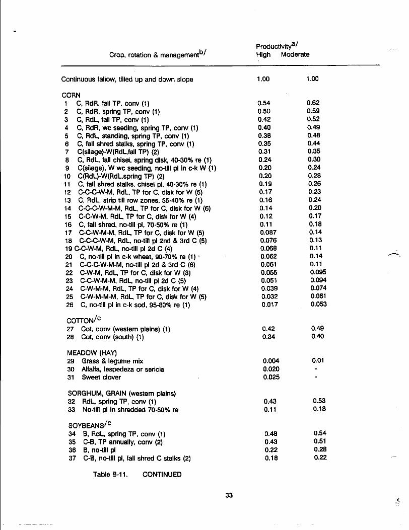
Crop, rotation & managementbf Productivny8/ High Moderate '

Continuous fallow, tilled up and down slope 1.00 1.00

CORN 1 C, RdR, fall TP, conv (1) 0.54 0.62 2 C, RdR, spring TP, conv (1) 0.50 0.59 3 C, Rdl, fall TP, conv (1) 0.42 0.52 4 C, RdR, we seeding, spring TP, conv (1) 0.40 0.49 5 C, Rdl, standing, spring TP, conv (1) 0.38 0.48 6 C, fall shred stalks, spring TP, conv (1) 0.35 0.44 7 C(sllage)-W(Rdl,fall TP) (2) 0.31 0.35 8 C, Rdl, fall chisel, spring disk, 40-30% re (1) 0.24 0.30 9 C(silage), W we seeding, no-till pi in c-k W (1) 0.20 0.24 10 C(Rdl)-W(Rdl,spring TP) (2) 0.20 0.28 11 C, fall shred stalks, chisel pi, 40-30% re (1) 0.19 0.26 12 C-C-C-W-M, Rdl, TP for C, disk for W (5) 0.17 0.23 13 C, Rdl, strip till row zones, 55-40% re (1) 0.16 0.24 14 C-C-C-W-M-M, Rdl, TP for C, disk for W (6) 0.14 0.20 15 C-C-W-M, Rdl, TP for C, disk for W (4) 0.12 0.17 16 C, fall shred, no-till pi, 70-50% re (1) 0.11 0.18 17 C-C-W-M-M, Rdl, TP for C, disk for W (5) 0.087 0.14 18 C-C-C-W-M, Rdl, no-till pi 2nd & 3rd C (5) 0.076 0.13 19 C-C-W-M, Rdl, no-till pi 2d C (4) 0.068 0.11 20 C, no-till pi in c-k wheat, 90-70% re (1) · 0.062 0.14 .-, 21 C-C-C-W-M-M, no-till pi 2d & 3rd C (6) 0.061 0.11 22 C-W-M, Rdl, TP for C, disk for W (3) 0.055 0.095 23 C-C-W-M-M, Rdl, no-till pi 2d C (5) 0.051 0.094 24 C-W-M-M, Rdl, TP for C, disk for W (4) 0.039 0.074 25 C-W-M-M-M, Rdl, TP for C, disk for W (5) 0.032 0.061 26 C, no-till pi In c-k sod, 95-80% re (1) 0.017 0.053

conoN/c 27 Cot, conv (western plains) (1) 0.42 0.49 28 Cot, conv (south) (1) 0;34 0.40

MEADOW (HAY) 29 Grass & legume mix 0.004 0.01 30 Alfalfa, lespedeza or sericia 0.020 31 Sweet clover 0.025

SORGHUM, GRAIN (western plains) 32 Rdl, spring TP, conv (1) 0.43 0.53 33 No-till pi in shredded 70-50% re 0.11 0.18

SOY8EANSfc 34 8, Rdl, spring TP, conv (1) 0.48 0.54 35 C-8, TP annually, conv (2) 0.43 0.51 36 8, no-till pi 0.22 0.28 37 C-8, no-till pi, fall shred C stalks (2) 0.18 0.22

Table 8-11. CONTINUED

33 :{ ..... "" ·'

- --- -- - -----------------

Crop, rotation & managementb/

WHEAT 38 W-F, fall TP after W (2) 39 W-F, stubble mulch, 500 lb re (2) 40 W-F, stubble mulch, 1000 Lb re (2) 41 Spring W, Rdl, Sept TP, conv (ND,SD) (1) 42 Winter W, Rdl, Aug TP, conv (KS) (1) 43 Spring W, stubble mulch, 750 lb re (1) 44 Spring W, stubble mulch, 1250 lb re (1) 45 Winter W, stubble mulch, 750 lb re (1) 46 Winter W, stubble mulch, 1250 lb re (1) 47 W-M, conv (2) 48 W-M-M, conv (3) 49 W-M-M-M, conv (4)

Productivitfl/ High Moderate

0.38 0.32 0.21 0.23 0.19 0.15 0.12 0.11 0.10 0.054 0.026 0.021

aj High level exemplified by long-term yield averages greater than 75 bujac corn or 3 tonjac hay or cotton management that regularly provides good stands and growth.

b/ Numbers in parentheses indicate numbers of years in the rotation cycle. (1) Indicates a continuous one-crop system.

cj Grain sorghum, soybeans or cotton may be substituted for corn in lines 12, 14, 15, 17-19, 21-25 to estimate values for sod-based rotations.

Abbreviations:

B soybeans F fallow c corn M grass & legume hay c-k chemically killed pi plant conv conventional w wheat cot cotton

lb re % re xx-yyo/o re RdR Rdl TP

Table B-11.

we winter cover

pounds of residue per acre remaining on surface after new crop seeding percentage of soil surface covered by residue mulch after new crop seeding XX% cover for high productivity, yy% for moderate. residues (corn stover, straw, etc.) removed or burned residues left on field (on surface or incorporated) turn plowed (upper 5 or more inches of soil inverted, covering residues

Generalized Values of Cover and Management Factor (C) for Field Crops East of the Rocky Mountains (Stewart.m..m., 1975).

34

-----------------

~----

Cover

Permanent pasture, idle land, unmanaged woodland

95-100% ground cover as grass as weeds

80% ground cover as grass as weeds

60% ground cover as grass as weeds

Managed woodland

75-100% tree canopy 40-75% tree canopy 20-40% tree canopy

Value

0.003 0.01

0.01 0.04

0.04 0.09

0.001 0.002-Q.004 0.003-Q.01

Table B-12. Values of Cover and Management Factor (C) for Pasture and Woodland (Novotny & Chesters, 1981).

Practice Slope(%): 1.1-2 2.1-7 7.1-12 12.1-18 18.1-24

No support practice 1.00 1.00 1.00 1.00 1.00

Contouring 0.60 0.50 0.60 0.80 0.90

Contour strip fropping R-R-M-Ma 0.30 0.25 0.30 0.40 0.45 R-W-M-M 0.30 0.25 0.30 0.40 0.45 R-R-W-M 0.45 0.38 0.45·· 0.60 0.68 R-W 0.52 0.44 0.52 0.70 0.90 R-0 0.60 0.50 0.60 0.80 0.90

Contour listing or ridge planting 0.30 0.25 0.30 0.40 0.45

Contour terracingb I 0.6/V'n 0.5jv'n 0.6/V'n o.8jv'n 0.9/V'n

aj R = row crop, W = fall-seeded grain, M = meadow. The crops are grown In rotation and so arranged on the field that row crop strips are always separated by a meadow or winter-grain strip.

b/ These factors estimate the amount of soil eroded to the terrace channels. To obtain off-field values, multiply by 0.2. n = number of approximately equal length intervals into which the field slope is divided by the terraces. Tillage operations must be parallel to the terraces.

Table B-13. Values of Supporting Practice Factor (P) (Stewart~ .• 1975).

35

__..-..!...,

Zone a/ Seasonb/

Location Cool Warm

1 2 3 4 5 6 7 8 9 10 11 12 13 14 15 16 17 18 19 20 21 22 23 24 25 26 27 28 29 30 31 32 33

Fargo NO 0.08 0.30 Sioux City lA 0.13 0.35 Goodland KS 0.07 0.15 Wichita KS 0.20 0.30 Tulsa OK 0.21 0.27 Amarillo TX 0.30 0.34 Abilene TX 0.26 0.34 Dallas TX 0.28 0.37 Shreveport LA 0.22 0.32 Austin TX 0.27 0.41 Houston TX 0.29 0.42 St. Paul MN 0.10 0.26 Uncoln NE 0.26 0.24 Dubuque lA 0.14 0.26 Grand Rapids Ml 0.08 0.23 Indianapolis IN 0.12 0.30 Parkersburg WV 0.08 0.26 Springfield MO 0.17 0.23 Evansville IN 0.14 0.27 Lexington KY 0.11 0.28 Knoxville TN 0.10 0.28 Memphis TN 0.11 0.20 Mobile AL 0.15 0.19 Atlanta GA 0.15 0.34 Apalachacola FL 0.22 0.31 Macon GA 0.15 0.40 Columbia SC 0.08 0.25 Charlotte NC 0.12 0.33 Wilmington NC 0.16 0.28 Baltimore MD 0.12 0.30 Albany NY 0.06 0.25 Caribou ME 0.07 0.13 Hartford CN 0.11 0.22

aj Zones given in Figure B-1.

b/ Cool season: Oct - Mar; Warm season: Apr - Sept.

Table B-14. Rainfall Erosivity Coefficients (a) for Erosivity Zones in Eastern U.S. (Selker et al., 1990).

Initial Conditions. Several initial conditions must be provided in the TRANSPRT.DAT file: initial unsaturated and shallow saturated zone soil moistures (U1 and ·s1 ), snowmelt water (SN1) and antecedent rain + snowmelt for the fiVe previous days. It Is likely that these values will be uncertain in many applications. However, they will not affect model results for more than the first month or two of the simulation period. It

* is generally most practical to assign arbitrary initial values (U for u1 and zero for the remaining variables) and to discard the first year of the simulation results.

36

Nutrient Parameters

. A sample set of nutrient parameters required for the data file NUTRIENT.DAT is given in Appendix D.

Although the GWLF model will be most accurate when nutrient data are calibrated to local conditions, a set of default parameters has been developed to facilitate uncalibrated applications. Obviously these parameters, which are average values obtained from published water pollution monitoring studies, are only approximations of conditions in any watershed.

Rural and Groundwater Sources. Solid-phase nutrients in sediment from rural sources can be estimated

Figure B-3.

' \ l

Highl.y diverse Insufficient data

~ 9. 95-9. 99X ~ 9. 19-9. 19X IIIIll > 9. 29Y.

Nitrogen in Surface 30 em of Soils (Parker ..m...m .• 1946; Mills et at., 1985).

as the average soil nutrient content multiplied by an enrichment ratio. Soil nutrient levels can be determinec from soil samples, soil surveys or general maps such as those given in Figures B-3 and B-4. A value of 2.C for the enrichment ratio falls within the mid-range of reported ratios and can be used in absence of more specific data (McElroy et al., 1976; Mills _u., 1985).

Default flow-weighted mean concentrations of dissolved nitrogen and phosphorus In agricultural runofl are given in Table B-15. The cropland and barnyard data are from multi-year storm runoff sampling studies in South Dakota (Dombush.m...m., 1974) and Ohio (Edwards et al., 1972). The concentrations for snowmelt runoff from fields with manure on the soil surface are taken from a manual prepared by U. S. Departmen• of Agriculture scientists (Gilbertson .m_m., 1979).

37 ... ·{{!: ,' ··: ...

Figure B-4.

II 9.19-9.19X

a.a~-a.agx IIIIII B.2B-B.3BX

P 20 5 in Surface 30 em of Soils (P 20 5 is 44% phosphorus) (Parker et al., 1946; Mills ~ .• 1985).

Default values for nutrient concentrations in groundwater discharge can be inferred from the U.S. Eutrophication Survey results (Omernik, 1977) given in Table B-16. These data are mean concentrations computed from 12 monthly streamflow samples in watersheds free of point sources. Since such limited sampling is unlikely to capture nutrient fluxes from storm runoff, the streamflow concentrations can be assumed to represent groundwater discharges to streams.

Dissolved nutrient data for forest runoff are essentially nonexistent. Runoff is a small component of streamflow from forest areas and studies of forest nutrient flux are based on streamflow rather than runoff sampling. Hence the only possible default option is the use of the streamflow concentrations from the ";;:: 90% Forest• category In Table B-16 as estimates of runoff concentrations.

Default values for urban nutrient accumulation rates are provided in Table B-17. These values were developed for Nonhern VIrginia conditions and are probably suitable for smaller and relatively new urban areas. They would likely underestimate accumulations in older large cities.

Seotic Svstems. Representative values for septic system nutrient parameters are given in Table B-18. Per capita nutrient loads in septic tank effluent were estimated from typical flows and concentrations. The EPA Design Manyal (U.S. Environmental Protection Agency, 1980) indicates 170 /jday as a representative wastewater flow from on-site wastewater disposal systems. Alhajjar et al. (1989) measured mean nitrogen and phosphorus concentrations in septic tank effluents of 73 and 14 mgj/, respectively. The latter concentration is based on use of phosphate detergents. When non-phosphate detergents are used, the concentration dropped to 7.9 mgj/. These concentrations were combined with the 170 /jday flow to produce the effluent

38

nutrient loads given in Table B-18.

Nutrient uptake by plants (generally grasses) growing over the sepfic system adsorption field are frankly speculative. Brown & Thomas (1978) suggest that if the grass clippings are harvested, nutrients from a septic system effluent can support at least twice the normal yield of grass over the absorption field. Petrovic & Cornman (1982) suggest that retention of turf grass clippings can reduce required fertilizer applications by 25%, thus implying nutrient losses of 75% of uptakes. It appears that a conservative estimate of nutrient losses from plant cover would be 75% of the nutrient uptake of from a normal annual yield of grass. Reed ~. (1988) reported that Kentucky bluegrass annually utilizes 200-270 kgjha nitrogen and 45 kg/h~ phosphorus. Using the 200 kgjha nitrogen value, and assuming a six month growing season and a 20 m per capita absorption area, an estimated 1.6 gjday nitrogen and 0.4 gjday phosphorus are lost by plant uptake on a per capita basis during the growing season. The 20 m2 adsorption area was based on per bedroom adsorption area recommendations by the U.S. Public Health Service for a soil with average percolation rate ( • 12 minjcm) (U.S. Public Health Service, 1967).

The remaining Information needed are the numbers of people served by the four different types of septic systems (normal, short-circuited, ponded and direct discharge). A starting point for this data will generally be estimates of the unsewered population in the watershed. Local public health officials may be able to estimate the fractions of systems within the area which are of each type. However, the most direct way of generating the information is through a septic systems survey.

39

~

Land Use Nitrogen Phosphorus (----------( mg/ I)-------------)

Fallowaf Coma/ Small grainsaf Haf!l Pasturea/ Bam yardsb/

2.6 2.9 1.8 2.8 3.0

29.3

Snowmelt runoff from manured landcf: Corn 12.2 Small grains 25.0 Hay 36.0

afDornbush et al. (1974)

b/Edwards et al. (1972)

0.10 0.26 0.30 0.15 0.25 5.10

1.90 5.00 8.70

cj Gilbertson et al. (1979); manure left on soil surface.

Table B-15. Dissolved Nutrients in Agricultural Runoff.

Watershed Concentrations (mgj/) Type Eastern U.S. Central U.S. Western U.S.

Nitrogenaf: <!: 90% Forest 0.19 0.06 0.07 <!: 75% Forest 0.23 0.10 0.07 <!: 50% Forest 0.34 0.25 0.18 <!: 50% Agriculture 1.08 0.65 0.83 <!: 75% Agriculture 1.82 0.80 1.70 <!: 90% Agriculture 5.04 0.77 0.71

Phosphorusb I: <!: 90% Forest 0.006 0.009 0.012 <!: 75% Forest 0.007 0.012 0.015 <!: 50% Forest 0.013 0.015 0.015 <!: 50% Agriculture 0.029 0.055 0.083 <!: 75% Agriculture 0.052 0.067 0.069 <!: 90% Agriculture 0.067 0.085 0.104

a/ Measured as total inorganic nitrogen.

b/ Measured as total orthophosphorus

Table 8-16. Mean Dissolved Nutrients Measured in Streamflow by the National Eutrophication Survey (Omemik, 1977).

40

Sus- Total Total Land Use pended BOD Nitrogen Phosphorus

Solids ( ------------------------- kg fha-day -------------------)

lmgervious Surfaces Single family residential l·~

Low density (unitsjha <..e:s) 2.5 0.15 0.045 0.0045 Medium density (units/ha ;;::: ~ 6.2 0.22 0.090 0.0112

Townhouses & apartments t•a... 6.2 0.22 0.090 0.0112 High rise residential 3.9 0.71 0.056 0.0067 Institutional 2.8 0.39 0.056 0.0067 Industrial 2.8 0.71 0.101 0.0112 Suburban shopping center 2.8 0.71 0.056 0.0067 Central business district 2.8 0.85 0.101 0.0112

Pervioy§ ~Yrfi~~!i Single family residential "~

Low density (unitsjha < .Q.:e) 1.3 0.08 0.012 0.0016 Medium density (unitsjha ;;::: 9-:5) 1.1 0.15 0.022 0.0039

Town houses & apartments a. a_ 2.2 0.29 0.045 0.0078 High rise residential 0.8 0.08 0.012 0.0019 I nstitutlonal 0.8 0.08 0.012 0.0019 Industrial 0.8 0.08 0.012 0.0019 Suburban shopping center 0.8 0.08 0.012 0.0019 Central business district 0.8. 0.08 0.012 0.0019

Table B-17. Contaminant Accumulation Rates for Northern Virginia Urban Areas (Kuo, et al., 1988).

Parameter

e, per capita daily nutrient load In septic tank effluent (g/day)

Value

Nitrogen 12.0 Phosphorus

Phosphate detergents use 2.5 Non-phosphate detergents use 1.5

urn, per capita daily nutrient uptake by plants during month m (gjday)

Nitrogen: Growing season 1.6 Non-growing season 0.0

Phosphorus: Growing season 0.4 Non-growing season 0.0

Table B-18. Default Parameter Values for Septic Systems.

41

~

APPENDIX C: VALIDATION STUDY

The GWLF model was tested by comparing model predictions with measured streamflow, sediment and nutrient loads from the West Branch Delaware River Basin during a three-year period (April, 1979 - March, 1982). The model was run using the four-year period April, 1978- March, 1982 and first year results were ignored to eliminate effects of arbitrary initial conditions.

CAttttOttSUILLE RESERVOIR

Figure C-1. West Branch Delaware River Watershed.

The 850 km2 watershed, which is shown in Figure C-1, is in a dairy farming area in southeast New York which consists of 30% agricultural, 67% forested and 2% urban land uses. The river empties into Cannonsville Reservoir, which is a water supply source for the City of New York.

The model was run for the four-year period using daily precipitation and temperature records from the U.S. Environmental Data and Information service weather station at Walton, NY. To test the usefulness of the default parameters presented previously, no attempt was made to calibrate the model. No water quality data from the watershed were used to estimate parameters. All transport and chemical parameters were obtained by the general procedures described in the Appendix B.

Water Qualttv Observations

Continuous streamflow records were available from a U.S. Geological Survey gauging station at Walton, NY. Nutrient and sediment data were collected, analyzed and summarized by the N.Y. State Department of Environmental Conservation (Brown .m...m .. 1985). During base flow conditions, samples were collected at approximately one-week intervals. During storm events, samples were collected at 2-4 hour intervals during hydrograph rise and at 6-8 hour intervals in the 2-3 days following flow peak. More frequent sampling was carried out during major snowmelt events. Total and dissolved phosphorus and sediment (suspended solids) data were collected from March, 1980 through March, 1982. The sampling periods for dissolved and total nitrogen were less extensive: March, 1980 - September, 1981 and January, 1981 - September, 1981,

42

respectively.

Mass fluxes were computed by multiplying sediment or nutrient concentrations in a sample by "a volume of water determined by numerically integrating flow over the period of time from half of the preceding sampling time interval through half of the following sampling time interval" (Brown et al., 1985).

Watershed Data

Land Uses. The parameters needed for the agricultural and forest source areas were estimated from a land use sampling procedure similar to that described by Haith & Tubbs (1981 ). U.S. Geological Survey 1 :24,000 topographic maps of the watershed were over1ain by land use maps derived from 1971-197 4 aerial photography. The maps were then over1aln by a grid with 1-ha cells which was the basis of the sampling procedure. The land uses were divided Into two general categories: forest and agriculture. Forest areas were subdivided Into forest brushland and mature forest, and agricultural areas were subdivided Into cropland, pasture and inactive agriculture. A random sample of 500 cells was taken, stratified over the two major land uses to provide more intense sampling of agricultural areas (390 samples~· 110 for forest).

For each agricultural sample, the following were recorded: land use (cropland, pasture or Inactive), soil type and length and gradient of the slope of the field in which the 1-ha sample was located. Crops were separated into two categories, corn or hay, since these two crops make up 99% of the county cropland.

Barnyard areas were identified from examination of conservation plans for 30 watershed dairy farm barnyards. Average earthen and roof drainage areas were 0.1306 ha and 0.0369 ha, respectively. These values were assumed representative of the watershed's 245 barnyards, producing total earth and roof drainage areas of 32 and 9 ha, respectively.

Urban land uses (low-density residential, commercial and industrial) were calculated from Delaware County tax maps. The impervious portions of these areas were 16%, 54% and 34% for residential, commercial and Industrial land uses, respectively.

Runoff Curve Numbers. In forest areas, curve numbers were selected by soil type, assuming "good" hydrologic condition. Agricultural curve numbers were selected based on soil type, crop, management practice (e.g., strip cropping) and hydrologic condition. All pasture, hay and corn-hay rotations were assumed to be in good condition. Inactive agricultural areas were assumed to be the same as pasture. Corn grown in continuous rotation was considered in poor condition. Cropland breakdown into hay, continuous corn and rotated corn was determined from county data assembled by Soil Conservation Service (1976) and confirmed from Bureau of the Census (1980).

Rural source areas and curve numbers are listed In Table C-1. These areas were subsequently aggregated for the GWLF input files into the large areas given in Table C-2. Urban and barnyard areas are also given in Table C-2. Curve numbers are area-weighted averages for each source area.

Erosion and Sediment Parameters. Data required for estimation of soil loss parameters for logging sites were obtained from a forestry survey (Siavicek, 1980). Logging areas were located from a 1979 aerial survey. Transects of the logging roads at these sites were measured for soil loss parameters Kk, (LS)k, Ck and Pk. and from this information an average Kk (LS)k Ck Pk value was calculated.

Soil erodibility factors (Kk) for agricultural land were obtained from the Soil Conservation Service. Cove! factors (C) were selected Table B-10 based on several assumptions. For com, the assumptions were thai all residues are removed from the fields {91% of the com in the county is used for silage (Bureau of thE Census, 1980)), and all fields are spring tum-plowed and In the high productivity class (Knoblauch, 1976) A moderate productivity was assumed for hay (Knoblauch, 1976). Supporting practice factors of P = 1 werf used for all source areas except strip crop com. Area-weighted Kk (LS)k Ck Pk values are given in Tabll C-2. Coefficients for daily rainfall erosivity were selected from Table B-13 for Zone 31 (Figure B-1) . J.

43

watershed sediment delivery ratio of 0.065 was determined from Figure B-2.

Soil Hydrologic Curve

Source Area Group Area(ha) Numbe,.S

Continuous com B 414 81 c 878 88

Rotated com B 620 78 c 1316 85

Strip crop com c 202 82

Hay B 2319 72 c 10690 81 D 76 85

Pasture B 378 61 c 4639 74 D 76 80

Inactive agriculture B 328 61 c 3227 74 D 126 80

Forest brushland B 3118 48 c 24693 65 D 510 73

Mature forest B 510 55 c 27851 70

aj Antecedent moisture condition 2 (CN2k)

Table C-1. Areas and Curve Numbers for Agricultural and Forest Runoff Sources for West Branch Delaware River Basin.

44

--- -·----···-----· ·--- ---···--

Land Use Area(ha) Curve Numbe~/ Erosion Productb/

Corn 3430 83.8 0.214 Hay 13085 79.4 0.012 Pasture 5093 73.1 0.016 Inactive

Agriculture 3681 73.1 0.017 Barnyards 41 92.2 Forest 56682 66.5 Logging Trails 20 0.217 Residential (Low Density)

Impervious 104 98.0 Pervious 546 74.0

Commercial Impervious 49 98.0 Pervious 41 74.0

Industrial Impervious 34 98.0 Pervious 67 74.0

aj Antecedent moisture condition 2 (CN2k).

b/Kk (LS)k Ck pk

Table C-2.

Land Use

Corn Hay Pasture Inactive

Agriculture Forest Logging Barn Yards Residential Commercial Industrial

Watershed Weighted Mean

Table C-3.

Aggregated Runoff Source Areas in West Branch Delaware River Basin.

Cover Coefficient Area(ha) May-Oct Nov-Apr

3430 1.0 0.3 13085 1.0 1.0 5093 1.0 1.0

3681 1.0 1.0 56682 1.0 0.3

20 0.3 0.3 41 0.3 0.3

650 0.84 0.84 90 0.46 0.46

101 0.66 0.66

82873 1.00 0.49

Evapotranspiration Cover Coefficients for West Branch Delaware River Basin.

45

,.---...._,

Other Transport Parameters. For purpose of curve number and evapotranspiration cover coefficient selection, the growing season was assumed to correspond to months during which mean air temperature is at least 10°C (May-October). Cover coefficients were selected from Table B-8 and are listed in Table C-3 along with the area-weighted watershed values. An average groundwater recession constant of r = 0.1 was determined from analysis of 30 hydrograph recessions from the period 1971 - 1978. The seepage constant (s) was assumed to *be zero, and the default value of 1 o em was used for unsaturated zone available soil moisture capacity U .

Nutrient Concentrations and Accumulation Rates. Using the soil nutrient values given in Figures B-3 and B-4 and the previously suggested enrichment ratio of 2.0 produced sediment nutrient concentrations of 3000 mgjkg nitrogen and 1300 mgjkg phosphorus. Rural dissolved nutrient concentrations were selected from Tables B-15 and B-16. Manure is spread on corn land in the watershed and hence the manured land concentrations were used for corn land runoff in snowmelt months (January- March). Inactive agricultural land was assumed to have nutrient concentrations midway between pasture and forest values. Urban nutrient accumulation rates from Table B-17 were used, with "Central business district" values used for commercial land.

Seotic Svstem Parameters. The default values for nutrient loads and plant uptake given in Table B-18 were used to model septic systems. The population served by each type of septic system was estimated by determining the percentage of the total number of systems falling within each class and multiplying by the year-round and seasonal (June- August) unsewered populations in the watershed. Table C-4 summarizes the population data for septic systems.

System Type

Normal Short-circuited Ponded Direct discharge

Percent of Total Population

86 1

10 3

Population Served Year-rouod Seasonala/

7572 88

881 264

1835 21

213 64

aj June - August

Table C-4. Estimated Populations Served by Different Septic System Types in West Branch Delaware River Basin.

The year-round unsewered population estimate for the watershed was based on 1980 Census data. These data were also used to determine the average number of people per household and the number of housing units used on a part-time basis. The seasonal population was then calculated by assuming the number of people per household was the same for seasonal and year-round residents.

A range of values for the current (1991) percentage of each type of system was supplied by the New York City Department of Environmental Protection (Personal Communication, J. Kane, New York City Department of Environmental Protection). A estimate of the percentages for the study period was determined by comparing the range of current values with the percentages from a survey of a neighboring area of Delaware County with construction practices and code enforcement similar to the West Branch Delaware River Watershed at the time of the study (Personal Communication, A. Lemley, Cornell University).

46

Point Sources. Point sources of nutrients are dissolved loads from five municipal and two industrial wastewater treatment plants. These inputs are 3800 kgjmo nitrogen and 825 kgjmo phosphorus (Brown & Rafferty, 1980; Dickerhoff, 1981). •

Complete data inputs for the validation simulation run are given in Appendix D.

Validation Results

The GWLF streamflow predictions are compared with observations in Figure C-2. It Is apparent that although the model mirrors the timing of observed streamflow, predictions for any particular month may have substantial errors. Accuracy is poorest for low flows, when predicted strearnflows are essentially zero due

Figure C-2.

-

West Branch Delaware River (4/79-3/82)

18.-----------------------------------------------~

16+-----------------------------~x~--------------~

14+--------------+~------------~----------------~

E 12+-------------~------------~--------------~ u .......,

~ 10+-------------~~----------~~---------------f~ 0

;;:: E 8~~-----r+---~+---------~-+~~---------4~ 0

~ 6+-~----~--~~--r-------r-~--~-r----~~~~~ Vl

4+-~----~~~r-~------~~+-~--~--~--~~~

2+---~--~----~--~----~--------~~--~------~

o~.,~~rr"~"~~~~~~rT~rT.-r+~~--.. -r~ A J A 0 0 F A J A 0 0 F A J A 0 0 F

Month

I x Observed - Predicted

Observed and Predicted Monthly Streamflow.

to the very simple lumped parameter groundwater model.

Model predictions and observations for total phosphorus and nitrogen are compared In Agures C-3 and C-4. Both sets of predictions match the variations in observations but under-predict the February, 1981 peak values by 35% and 26% for phosphorus and nitrogen, respectively. A quantitative summary of the comparisons of predictions with observations is given In Table C-5. Monthly mean predictions are within 10% of observation means for five of the six model outputs. The predicted mean total nitrogen flux is 73% of the observed mean. No coefficient of determination (R2) is less than 0.88, indicating that the model explains at least 88% of the observed monthly variation in streamflow, sediment yield and nutrient fluxes.

Mean annual nutrient loads from each source for the four-year simulation period are provided In Table C-6. It Is apparent that cropland runoff Is a major source of streamflow nitrogen and phosphorus. Groundwater discharge Is the largest source of nitrogen, accounting for 41% of dissolved and 36% of total nitrogen loads. Point sources constitute 11% of total nitrogen and 20% of total phosphorus. Septic tank drainage provides nearly as much nitrogen as point sources, but is a minor phosphorus source.

47

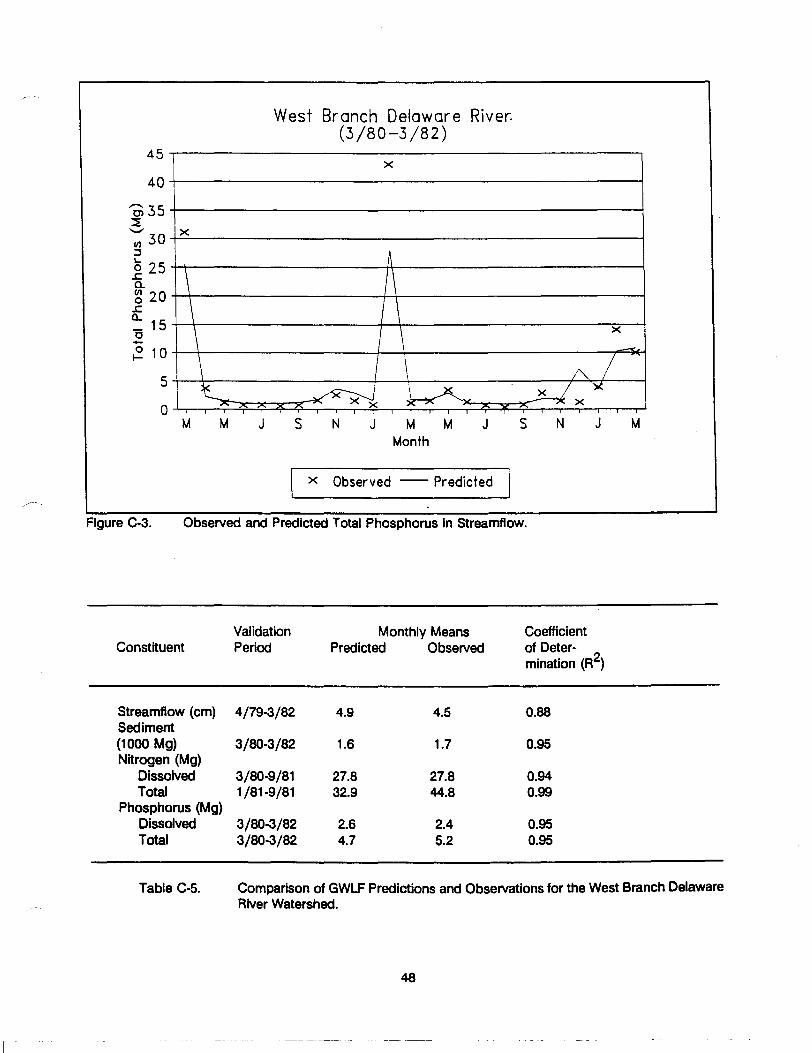
45

40

0;35 ~ "'-./

II) 30 ::::1

a 2s .c. a. ~ 20 .c. ~ 15 0 -(3. 1 0

5

0

X

\ \ \ \ ~

-"'

M M J

West Branch Delaware River. (3/80-3/82)

s X X

N J

X

A

\ \ \ \ '

~--M

Month M J

x Observed -- Predicted

X

.--.

;"'-., I _p_fx'X

s N J M

Figure C-3. Observed and Predicted Total Phosphorus in Streamflow.

Constituent

Streamflow (em) Sediment (1000 Mg) Nitrogen (Mg)

Dissolved Total

Phosphorus (Mg) Dissolved Total

Table C-5.

Validation Period

4/79-3/82

3/80-3/82

3/80-9/81 1/81-9/81

3/80-3/82 3/80-3/82

Monthly Means Predicted Observed

4.9 4.5

1.6 1.7

27.8 27.8 32.9 44.8

2.6 2.4 4.7 5.2

Coefficient of Determination (R2)

0.88

0.95

0.94 0.99

0.95 0.95

Comparison of GWLF Predictions and Observations for the West Branch Delaware River Watershed.

48

250

200

~ 150 Ol 0 !.... -z 100 0 -0 1-

50

0

Figure C-4.

Conclusions

X

1\

West Branch Delaware River ( 1 I 8 1 -9 I 8 1 )

1\ I \

j \_ ....

X

X ~""'

J F M A M Month

J

x Observed -- Predicted

Observed and Predicted Total Nitrogen in Streamflow.

J

X

A s

The watershed loading functions model GWLF is based on simple runoff, sediment and groundwater relationships combined with empirical chemical parameters. The model is unique in its ability to estimate monthly nutrient fluxes in streamflow without calibration. Validation studies in a large New York watershed indicated that the model possesses a high degree of predictive accuracy. Although better results could perhaps be obtained by more detailed chemical simulation models, such models have substantially greater data and computational requirements and must be calibrated from water quality sampling data.

The GWLF model has several limitations. Peak monthly nutrient fluxes were underestimated by as much as 35%. Since nutrient chemistry is not modeled explicitly, the model cannot be used to estimate the effects of fertilizer management or urban storm water storage and treatment. The model has only been validated for a largely rural watershed in which agricultural runoff and groundwater discharge provided most of the nutrient load. Although the urban runoff component is based on well-known relationships which have been used previously in such models as STORM and SWMM, GWLF performance in more urban watersheds is uncertain.

49

Source

Corn Hay Pasture Inactive

Agriculture Forest & logging Barn yards Urban

Nitrogen (Mg) Dissolved Total

52.9 84.6 48.6 55.4 13.2 16.7

5.1 7.8 5.9 6.1 4.3 4.3

2.8

Phosphorus (Mg) Dissolved Total

7.8 21.5 2.6 5.5 1.1 2.6

0.4 1.6 0.2 0.3 0.8 0.8

0.3

Groundwater. Point Sources. & Seotic Systems

Groundwater Discharge

Point sources Septic systems

Watershed Total

Table C-6.

149.6 45.6 38.1

363.4

149.6 45.6 38.1

411.1

5.7 9.9 1.1

29.6

5.7 9.9 1.1

48.3

Mean Annual Nutrient Loads Estimated from GWLF for the West Branch Delaware River Watershed: 4/78- 3/82.

50

APPENDIX D: DATA AND OUTPUT LISTINGS FOR VALIDATION STUDY (EXAMPLE 1)

The first listing in this appendix is the set of sequential data input files TRANSPRT.DAT, NUTRIENT.DAT and WEATHER.DAT used in the validation study and Example 1. The first two files are constructed by selecting the appropriate option from GWLF menus. The weather file is arranged by months (April -March, in this application) with the first entry for each month being the number of days in the month, and subsequent entries being temperature (0 C) and precipitation (em) for each day. Only a partial listing of WEATHER.DAT is given. The next listings are the text files for the transport and nutrient data (TRANSPRT.TXT and NUTRIENT.TXT). The remaining listings are text files of the several program outputs (SUMMARY.TXT and MONTHLY.TXT).

51

TRANSPRT.DAT

7,6 .1,0,10,0,0, .065,10 0 0 0 0 0 "APR", . 49, 13.1, 0, . 25 "MAY",1,14.3,1,.25 "JUNE",1,15,1, .25 "JULY", 1,14. 6,1,. 25 "AUG",1,13.6,1, .25 "SEPT",1,12.3,1, .25 "OCT",1,10.9,1, .06 "NOV" , . 49, 9. 7 , 0, . 06 "DEC", .49,9,0, .06 "JAN",. 49,9. 3, 0,. 06 "FEB", .49,10.4,0, .06 "MAR", .49, 11.7, 0,. 06 "CORN", 3430, 8:L8,. 214 "HAY", 13085, i9. 4, . 012 "PASTURE",5093,73.1, .016 "INACTIVE", 3681,73 .1,. 017 "FOREST",56682,66.5,0 "LOGGING",20,0, .217 "BARN YARDS",41,92.2,0 "RES-imperv",104,98,0 "RES-perv",546,74,0 "COMM-imperv",49,98,0 "COMM-perv",41,74,0 "INDUS-imperv",34,98,0 "INDUS-perv",67,74,0

NUTRIENT.DAT

3000,1300, .34, .013 1,10,12 2. 9,. 26 2. 8' .15 3'. 25 1. 6' .13 .19'. 006 0,0 29.3,5.1 0. 045 '0. 0045) 0. 012' 0. 0016 ( 0. 101' 0. 0112 -i 0. 012 '0. 0019 ' 0 .101, 0. 0112 / 0.012,0.0019/ 12.2' 1. 9 :: 3800,825' 3800,825 3800,825 3800,825 3800,825 3800,825 3800' 825 ,.-3800,825 3800,825 3800,825 3800,825 3800' 825 --1 7572,881,88,264 7572,881,88,264 9407,1094,109,328 9407,1094,109,328 9407,1094,109,328 7572,881,88,264 7572,881,88,264 7572,881,88,264 7572,881,88,264 7572,881,88,264 7572,881,88,264 7572,881,88,264 12,2.5,1.6,.4 /

52

,/'

/

WEATHER.DAT

30 11, .2 2, .4 -3' .1 2,0 3,1 4,0 9, .4 2, .1 2, .1 4,0 12' .1 10,. 6 12,0 5' .1 2, .1 5,0 4,0 5' .1 7,0 8' 1. 3 4, .4 6' .1 4,0 6,0 7,0 8,0 9,0 8,0 7,0 5, .1 31' -1,0 6,0 6,0 5,0 7'. 3., 6' 1.3 11, .6 9,0 15' .8 10,. 2 15,0 13,0 16,0 14,0 12, .5 11, .4 11, .8 14, .4 17' .2 • • •

TRANSPRT.TXT

TRANSPRT DATA

lAND USE AREA(ha) CURVE NO CORN 3430. 83.8 HAY 13085. 79.4 PASTURE 5093. 73.1 INACTIVE 3681. 73.1 FOREST 56682. 66.5 LOGGING 20. 0.0 BARN YARDS 41. 92.2 RES-imperv 104. 98.0 RES-perv 546. 74.0 COMM- imperv 49. 98.0 COMM-perv 41. 74.0 INDUS-imperv 34. 98.0 INDUS-perv 67. 74.0

MONTH ET CV() DAY HRS GROW. SEASON APR 0.490 13.1 0 MAY 1.000 14.3 1 JUNE 1.000 15 1 JULY 1.000 14.6 1 AUG 1.000 13.6 1 SEPT 1.000 12.3 1 OCT 1.000 10.9 1 NOV 0.490 9.7 0 DEC 0.490 9 0 JAN 0.490 9.3 0 FEB 0.490 10.4 0 MAR 0.490 11.7 0

ANTECEDENT RAIN+MELT FOR DAY -1 TO DAY -5 0 0 0 0 0

INITIAL UNSATURATED STORAGE (em) - 10 INITIAL SATURATED STORAGE (em) 0 RECESSION COEFFICIENT (1/day) .1 SEEPAGE COEFFICIENT (1/day) 0 INITIAL SNOW (em water) 0 SEDIMENT DELIVERY RATIO - O.Of~ UNSAT AVAIL WATER CAPACITY (em) 10

NUTRIENT.TXT

RURAL LAND USE CORN HAY PASTURE INACTIVE FOREST LOGGING BARN YARDS

NUTRIENT DATA

DIS.NITR IN RUNOFF(mg/1) 2.9 2.8 3 1.6 .19 0 29.3

53

KLSCP 0.21400 0.01200 0.01600 0.01700 0.00000 0.21700 0.00000 0.00000 0.00000 0.00000 0.00000 0.00000 0.00000

EROS. COEF .25 .25 .25 .25 .25 .25 .06 .06 .06 .06 .06 .06

DIS.PHOS IN RUNOFF(mg/1) .26 .15 .25 .13 .006 0 5.1

-------

NUTRIENT CONCENTRATIONS IN RUNOFF FROM MANURED AREAS

LAND USE CORN

NITROGEN(mg/1) 12.2

PHOS~HORUS(mg/1) 1.9

URBAN LAND USE RES-imperv RES-perv

NITR. BUILD-UP (kgjha- day). .045

PHOS.BUILD-UP(kg/ha-day) .0045

COMM- imperv COMM-perv INDUS-imperv INDUS-perv

.012

.101

.012

.101

.012

.0016

.0112

.0019

.0112

.0019

MONTH APR MAY JUNE JULY AUG SEPT OCT NOV DEC JAN FEB MAR

POINT SOURCE NITR.(kg) 3800

POINT SOURCE PHOS.(kg) 825

3800 3800 3800 3800 3800 3800 3800 3800 3800 3800 3800

NITROGEN IN GROUNDWATER (mg/1): PHOSPHORUS IN GROUNDWATER (mg/1): NITROGEN IN SEDIMENT (mgjkg): PHOSPHORUS IN SEDIMENT (mg/kg):

MANURE SPREADING JAN THRU MAR

SEPTIC SYSTEMS

0.340 0.013

3000 1300

POPULATION SERVED

825 825 825 825 825 825 825 825 825 825 825

NORMAL SYSTEMS

7572 7572 9407 9407 9407 7572 7572 7572 7572 7572 7572 7572

PONDING SHORT-CIRCUIT MONTH APR MAY JUNE JULY AUG SEPT OCT NOV DEC JAN FEB MAR

SYSTEMS SYSTEMS 881 88 881 88 1094 109 1094 109 1094 109 881 88 881 88 881 88 881 88 881 88 881 88 881 88

PER CAPITA TANK EFFLUENT NITROGEN (g/day) 12 PER CAPITA TANK EFFLUENT PHOSPHORUS (g/day) 2.5 PER CAPITA GROWING SEASON NITROGEN UPTAKE (g/day) 1.6 PER CAPITA GROWING SEASON PHOSPHORUS UPTAKE (g/day) - .4

54

DISCHARGE SYSTEMS

264 264 328 328 328 264 264 264 264 264 264 264

SUMMARY.TXT

W. Branch Delaware River 4/78-3/82 .

4 -year means

PRECIP EVAPOTRANS GR.WAT.FLOW RUNOFF STREAMFLOW - - - - - - - - - - - - - - - - - ( em) - - - - - - - - - - - - - - - - - - - - - - - - - - - - - - - - - -

APR 9.6 1.9 6.5 0.3 6.7 MAY 9 . 8 7 . 5 5 . 3 0 . 3 5 . 6 JUNE 8 . 3 9 . 7 1. 8 0 . 0 1. 8 JULY 8 . 6 11. 3 0 . 1 0 . 0 0 . 2 AUG 10. 4 9. 2 1. 2 0. 9 2. 0 SEPT 11.6 5. 8 0.1 0.1 0. 2 OCT 11. 5 3. 1 4. 3 0 .1 4. 4 NOV 8 . 2 0 . 7 6 . 6 0 . 4 7 . 0 DEC 8 . 0 0 . 2 5 . 6 0. 4 6 . 0 JAN 8.1 0.1 5. 0 1.1 6.1 FEB 8.5 0.2 5.7 1.8 7.4 MAR 9 . 8 0. 8 10. 9 2. 4 13. 3 ---------------------------------------------------------------ANNUAL 112.3 50.7

APR MAY JUNE JULY AUG SEPT OCT NOV DEC JAN FEB MAR

EROSION SEDIMENT ----(1000 Mg)----29.2 0.0 35.7 0.2 23.5 0. 0 28.1 0.0 45.8 1. 2 45.0 0.0 11.2 0.1

6. 3 0. 9 0.8 1.1 0.4 1.1 0.5 4.4 3. 7 6.0

53.1 7.8 60.8

DIS.NITR TOT.NITR DIS.PHOS TOT.PHOS ------------(Mg)------------------

30.7 31.1 1.9 2.0 26.9 27.7 1.8 2.1 10.7 10.9 1.1 1.2 4.9 5.2 1.0 1.0

17.2 21.0 1.7 3.2 6.2. 6.6 1.1 1.1

21.3 21.8 1.6 1.7 33.3 36.1 2.1 3.2 28.9 32.3 1.9 3.3 41.4 45.0 3.6 5.1 55.4 68.8 4.9 10.6 86.6 104.8 7.0 14.8

----------------------------------------------------------------ANNUAL 230.4 15.0 363.4 411.0 29.6 49.3

SOURCE AREA (ha)

3430. 13085.

5093. 3681.

56682.

RUNOFF (em)

18.03 13.27

8.65 8.65 5.47 0.00

EROSION (Mgjha)

DIS.NITR TOT.NITR DIS.PHOS TOT.PHOS

CORN HAY PASTURE INACTIVE FOREST LOGGING BARN YARDS RES-imperv RES-perv COMM-imperv COMM..,perv INDUS-imperv INDUS-perv GROUNDWATER POINT SOURCE SEPTIC SYSTEMS

20. 41.

104. 546. 49. 41. 34. 67.

36.11 74.11

9.20 74.11

9.20 74.11 9.20

47.43 2.66 3.55 3. 77 0.00

48.10 0.00 0.00 0.00 0.00 0.00 0.00 0.00

--------------(Mg)------------52.92. 84.64 7.78 21.52 48.60 55.39 2.60 5.54 13.22 16.74 1.10 2.63

5.10 7.80 0.41 1.59 5.89 5.89 0.19 0.19 0.00 0.19 0.00 0.08 4.34 4.34 0.76 0.76 0.00 0.86 0.00 0.~9 0.00 0.29 0.00 0.04 0.00 0.91 0.00 0.10 0.00 0.02 0.00 0.00 0.00 0.63 0.00 0.07 0.00 0.04 0.00 0.01

149.58 149.58 5.72 5.72 45.60 45.60 9.90 9.90 38.13 38.13 1.11 1.11

---------------------------------------------------------------------------TOTAL 363.37 411.05 29.57 49.34

55

MONTHLY.TXT

W. Branch Delaware River 4/78-3/82 YEAR 1

PRECIP EVAPOTRANS GR.WAT.FLOW RUNOFF STREAMFLOW -----------------(cm)----------------------------------

APR 5.2 1.7 3.1 0.0 3.1 MAY 7.9 7.4 2.1 0.0 2.1 JUNE 10 . 5 9 . 7 1. 8 0 . 0 1. 8 JULY 10. 8 10. 9 0. 3 0. 0 0. 4 AUG 17.0 10.4 4.6 3.4 8.1 SEPT 7.6 5.5 0.4 0.1 0.4 OCT 11.6 3.1 3.9 0.0 3.9 NOV 4 . 7 0 . 7 3 . 7 0 . 1 3 . 8 DEC 12.6 0.2 5.2 0.0 5.2 JAN 19.1 0.2 8.7 3.8 12.6 FEB 4.0 0.1 4.6 0.5 5.1 MAR 10.9 1.1 16.5 4.6 21.0 ---------------------------------------------------------------YEAR 121.9 50.9 54.9 12.6 67.4

EROSION SEDIMENT ----(1000 Mg)----

DIS.NITR TOT.NITR DIS.PHOS TOT.PHOS

8.3 0.0 ------------(Mg)------------------

14. 9 15 . 0 1. 3 1. 3 13.3 0.0 11.3 11.5 1.1 1.2 29.3 0.0 10.8 11.0 1.2 1.2 39.4 0.0 5.8 6.1 1.0 1.0

109.6 4.7 54.9 69.5 3.8 10.0 35.4 0.0 6.8 6.9 1.1 1.1 10.3 0.0 17.8 18.i 1.4 1.4 1.4 0.0 18.2 18.4 1.4 1.4 1.8 0.0 22.1 22.3 1.5 1.5

APR MAY JUNE JULY AUG SEPT OCT NOV DEC JAN FEB MAR

0.0 3.8 100.4 112.2 8.9 13.9 0.0 0.2 32.7 33.5 2.8 3.1 5.0 7.7 139.6 163.2 11.2 21.3

----------------------------------------------------------------YEAR 253.8 16.5 435.3 487.5 36.6 58.3

SOURCE

CORN HAY PASTURE INACTIVE FOREST

AREA (ha)

3430. 13085.

5093. 3681.

56682. LOGGING BARN YARDS RES-imperv RES-perv COMM-imperv COMM-perv INDUS-imperv INDUS-perv GROUNDWATER POINT SOURCE SEPTIC SYSTEMS

20. 41.

104. 546.

49. 41. 34. 67.

RUNOFF (em)

24.70 19.27 13.86 13.86

9.81 0.00

44.22 82.95 14.52 82.95 14.52 82.95 14 .. 52

EROSION DIS.NITR TOT.NITR DIS.PHOS TOT.PHOS (Mg(ha) --------------(Mg)------------

52.26 81.18 116.13 12.18 27.33 2.93 70.59 78.06 3.78 7.02 3.91 21.18 25.06 1.76 3.45 4.15 8.16 11.14 0.66 1.95 0.00 10.57 10.57 0.33 0.33

52.99 0.00 0.21 0.00 0.09 0.00 5.31 5.31 0.92 0.92 0.00 0.00 0.86 0.00 0.09 0.00 0.00 0.30 0.00 0.04 0.00 0.00 0.90 0.00 0.10 0.00 0.00 0.02 0.00 0.00 0.00 0.00 0.63 0.00 0.07 0.00 0.00 0.04 0.00 0.01

154.61 ~54.61 5.91 5.91 45.60 45.60 9.90 9.90 38.10 38.10 1.11 1.11

---------------------------------------------------------------------------TOTAL 435.30 487.55 36.58 58.33

56


PRECIP EVAPOTRANS GR.WAT.FLOW RuNOFF STREAMFLOW -----------------(em)----------------------------------

APR 11.0 1.8 8.5 0.7 9.2 MAY 15.3 7.6 6.8 0.6 7.5 JUNE 4.2 9.6 3.8 0.0 3.8 JULY 7.2 11.5 0.2 0.0 0.2 AUG 9.2 7.6 0.0 0.0 0.0 SEPT 14.3 6.0 0.0 0.1 0.1 OCT 11.2 3.4 6.7 0.1 6.7 NOV 13.5 0.9 8.6 0.8 9.4 DEC 5.0 0.4 6.7 0.0 6.7 JAN 3.7 0.2 4.3 0.0 4.3 FEB 4.0 0.1 1.4 0.0 1.4 MAR 14.8 0.7 10.7 3.0 13.7 ---------------------------------------------------------------YEAR 113.4 49.8 57.6 5.4 63.0

EROSION SEDIMENT DIS.NITR TOT.NITR DIS.PHOS TOT.PHOS ----(1000 Mg)---- ------------(Mg)------------------

APR 35.1 0.2 43.4 44.2 2.6 2.8 MAY 66.9 0.5 37.6 39.3 2.4 3.1 JUNE 11.2 0.0 17.2 17.3 1.3 1.4 JULY 15.4 0.0 4.9 5.1 0.9 1.0 AUG 19.1 0.0 4.4 4.6 0.9 1.0 SEPT 64.7 0.1 6.5. 7.0 1.1 1.2 OCT 8.2 0.0 27.9 28.2 1.7 1.8 NOV 21.0 2.6 45.2 53.3 2.7 6.1 DEC 0.7 0.0 27.6 27.9 1.7 1.7 JAN 1.7 0.0 18.9 19.0 1.4 1.4 FEB 0.0 0.0 10.2 10.3 1.2 1.2 MAR 8.6 13.0 99.0 138.5 8.5 25.5

YEAR 252.7 16.4 342.6 394.6 26.4 48.1

SOURCE

CORN HAY PASTURE INACTIVE FOREST LOGGING BARN YARDS RES-imperv RES-perv

AREA (ha)

3430. 13085.

5093. 3681.

56682. 20. 41.

104. 546.

49.

RUNOFF (em)

15.22 10.54

6.11 6.11 3.26 0.00

COMM- imperv COMM-perv INDUS-imperv INDUS-perv GROUNDWATER POINT SOURCE SEPTIC SYSTEMS

41. 34. 67.

33.71 74.86 6.62

74.86 6.62

74.86 6.62

EROSION DIS.NITR TOT.NITR DIS.PHOS TOT.PHOS (Mgjha) --------------(Mg)------------

52.02 37.28 72.08 5.26 20.34 2.92 38.60 46.05 2.07 5.29 3.89 9.33 13.19 0.78 2.45 4.13 3.60 6.56 0.29 1.58 0.00 3.51 3.51 0.11 0.11.

52.75 0.00 0.21 0.00 0.09 0.00 4.05 4.05 0.70 0.70 0.00 0.00 0.88 0.00 0.09 0.00 0.00 0.28 0.00 0.04 0.00 0.00 0.93 0.00 0.10 0.00 0.00 0.02 0.00 0.00 0.00 0.00 0.64 0.00 0.07 0.00 0.00 0.03 0.00 0.01

162.40 162.40 6.21 6.21 45.60 45.60 9.90 9.90 38.21 38.21 1.12 1.12

---------------------------------------------------------------------------TOTAL 342.59 394.64 26.44 48.10

57

------.

/-


PRECIP EVAPOTRANS GR.WAT.FLOW RUNOFF' STREAMFLOW - - - - - - - - - - - - - - - - - (em) - - - - - - - - - - - - - - - - - - - - - - - - - - - - - - - - - -

APR 11.9 2.1 9.3 0.2 9.5 MAY 3.2 7.6 4.3 0.0 4. 3 JUNE 10.4 9.1 0.2 0.0 0.2 JULY 9.5 11.5 0.0 0.0 0.0 AUG 9.9 10.3 0.0 0.0 0.0 SEPT 10.7 6.3 0.0 0.2 0.2 OCT 10.0 3.0 2.2 0.2 2.4 NOV 8.8 0.5 6.7 0.9 7.6 DEC 6.3 0.1 6.2 0.6 6.8 JAN 2.8 0.0 2.4 0.1 2.5 FEB 16.8 0.6 10.7 5.1 15.8 MAR 4.3 0.8 5.9 0.0 5.9 ---------------------------------------------------------------YEAR 104.6 52.0 47.8 7.4 55.2


APR 45.5 0.0 40.9 41.2 2.2 2.3 MAY 6.7 0.0 19.2 19.3 1.4 1.4 JUNE 38.2 0.0 5.4 5.7 1.0 1.0 JULY 37.6 0.0 4.5 4.7 1.0 1.0 AUG 41.7 0.0 5.2 5.4 1.0 1.0 SEPT 36.6 0.1 7.1 7.5 1.1 1.2 OCT 15.9 0.1 16.3 17.0 1.5 1.7 NOV 0.5 0.8 40.3 43.1 2.5 3.6 DEC 0.2 0.6 33.9 35.8 2.1 2.9 JAN 0.0 0.0 15.6 15.8 1.5 1.6 FEB 2.1 13.0 126.8 166.2 11.1 28.0 MAR 0.7 0.0 25.7 26.0 1.7 1.7

YEAR 225.7 14.7 340.9 387.6 28.1 47.5

SOURCE

CORN HAY PASTURE INACTIVE FOREST

AREA (ha)

3430. 13085.

5093. 3681.

56682. LOGGING BARN YARDS RES-imperv RES-perv COMM-imperv COMM-perv INDUS-imperv INDUS-perv GROUNDWATER POINT SOURCE SEPTIC SYSTEMS

TOTAL

20. 41.

104. 546. 49. 41. 34. 67.

RUNOFF (em)

17.55 12.74

·8 .17 8.17 5.14 0.00

35.45 70.37 8.69

70.37 8.69

70.37 8.69

EROSION DIS.NITR TOT.NITR DIS.PHOS TOT.PHOS (Mg/ha) --------------(Mg)------------

46.48 48.63 79.72 7.06 20.53 2.61 46.69 53.34 2.50 5.38 3.47 12.48 15.93 1.04 2.54 3.69 4.81 7.46 0.39 1.54 0.00 5.54 5.54 0.17 0.17

47.13 0.00 0.18 0.00 0.08 0.00 4.26 4.26 0.74 0.74 0.00 0.00 0.85 0.00 0.08 0.00 0.00 0.28 0.00 0.04 0.00 0.00 0.90 0.00 0.10 0.00 0.00 0.02 0.00 0.00 0.00 0.00 0.62 0.00 0.07 0.00 0.00 0.03 0.00 0.01

134.79 134.79 5.15 5.15 45.60 45.60 9.90 9.90 38.10 38.10 1.11 1.11

340.89 387.61 28.08 47.45

58


PRECIP EVAPOTRANS GR.WAT.FLOW RUNOFF STREAMFLOW - - - - - - - - - - - - - - - - - (em) - - - - - - - - - - - - - - - - - - - - - - - - - - - - - - - - - -

APR 10.3 2.1 5.0 0.1 5.1 MAY 13.0 7.4 8.1 0.5 8.6 JUNE 8.1 10.4 1.4 0.0 1.4 JULY 7.0 11.4 0.1 0.0 0.1 AUG 5.4 8.7 0.0 0.0 0.0 SEPT 13.7 5.4 0.0 0.0 0.0 OCT 13.1 2.9 4.6 0.2 4.7 NOV 5.9 0.7 7.3 0.0 7.3 DEC 8.2 0.1 4.3 1.1 5.5 JAN 6.6 0.1 4.6 0.4 5.0 FEB 9.1 0.1 5.9 1.5 7.4 MAR 9.0 0.7 10.7 1.8 12.5

YEAR 109.4 50.0 52.0 5.7 57.7


APR 28.0 0.0 23.5 23.9 1.6 1.7 MAY 55.8 0.4 39.3 40.8 2.3 2.9 JUNE 15.4 0.0 9.3 9.4 1.1 1.1 JULY 20.1 0.0 4.6 4.8 0.9 1.0 AUG 12.7 0.0 4. 3 4.5 0.9 0.9 SEPT 43.2 0.0 4.6 4.9 1.0 1.0 OCT 10.5 0.2 23.0 23.8 1.6 1.9 NOV 2.4 0.0 29.5 29.7 1.7 1.7 DEC 0.5 3.6 32.0 43.2 2.2 7.0 JAN 0.0 0.7 30.6 32.9 2.6 3.5 FEB 0.0 4. 3 51.9 65.1 4.5 10.1 MAR 0.7 3.1 82.0 91.6 6.7 10.7 ----------------------------------------------------------------YEAR 189.3 12.3 334.7 374.4 27.2 43.5

SOURCE

CORN HAY PASTURE INACTIVE FOREST LOGGING BARN YARDS RES-imperv RES-perv

AREA (ha)

3430. 13085.

5093. 3681.

56682.

COMM- imperv COMM-perv INDUS-imperv INDUS-perv GROUNDWATER POINT SOURCE SEPTIC SYSTEMS

20. 41.

104. 546. 49. 41. 34. 67.

RUNOFF (em)

14.66 10.52

6.48 6.48 3.67 0.00

31.05 68.27

6.96 68.27

6.96 68.27

6.96

EROSION DIS.NITR TOT.NITR DIS.PHOS TOT.PHOS (Mg/ha) --------------(Mg)------------

38.98 ~4.57 70.64 6.60 17.89 2.19 8.54 44.12 2.06 4.48 2.91 9.90 12.79 0.82 2.08 3.10 3.81 6.04 0.31 1.27 0.00 3.95 3.95 0.12 0.12

39.52 0.00 0.15 0.00 0.07 0.00 3.73 3.73 0.65 0.65 0.00 0.00 0.87 0.00 0.09 0.00 0.00 0.30 0.00 0.04 0.00 0.00 0.92 0.00 0.10 0.00 0.00 0.02 0.00 0.00 0.00 0.00 0.64 0.00 0.07 0.00 0.00 0.04 0.00 0.01

146.50 146.50 5.60 5.60 45.60 45.60 9.90 9.90 38.10 38.10 1.11 1.11

---------------------------------------------------------------------------TOTAL 334.70 374.40 27.18 43.49

59

____....._

-J it ...... _;..., .......

REFERENCES

Alhajjar, B. J., Harkin, J. H., Chesters, G. 1989. Detergent formula and characteristics of wastewater in septic tanks. Journal of the Water Pollution Control Federation 61 (5): 605-613.

Amy, G., Pitt, R., Singh, R., Bradford, W. L., LaGraffi, M. B. 1974. Water quality management planning for urban runoff. EPA-440/9-75-Q04. U.S. Environmental Protection Agency, Washington DC.

Bosen, J. F. 1960. A formula for approximation of saturation vapor pressure over water. Monthly Weather Reviews 88(8):275-276).

Brown, K. W., Thomas, J. C. 1978. Uptake of N by grass from septic fields in three soils. Agronomy Journal 70(6)\ 1037-1040.

Brown, M. P., Rafferty, M.R. 1980. A historical perspective of phosphorus loading to the Cannonsville Reservoir as it relates to the West Branch Delaware River Model Implementation Program. Technical Report 62. N.Y. Department of Environmental Conservation, Albany NY.

Brown, M. P., Rafferty, M. R., Longabucco, P. 1985. Nonpoint source control of phosphorus- a watershed evaluation. Report to the U.S. Environmental Protection Agency, Ada, OK.

Bureau of the Census. 1980. 1978 census of agriculture, Delaware County, NY. U.S. Department of Commerce, Washington, DC.

Chow, V. T. 1964. Runoff. In: V. T. Chow (ed.). Handbook of Applied Hydrology. McGraw-Hill, New York NY, Chapter 14.

Davis, C. V., Sorensen, K. E. 1969. Handbook of Applied Hydraulics. McGraw-Hill, New York NY.

Delwiche, L. L D., Haith, D. A. 1983. Loading functions for predicting nutrient losses from complex watersheds. Water Resources Bulletin 19(6):951-959.

Dickerhoff, L. L. 1981. A methodology for predicting runoff and nutrient losses from a heterogeneous watershed. M. S. Dissertation. Department of Agricultural Engineering, Cornell University, Ithaca NY.

Dornbush, J. N., Anderson, J. R., Harms L L 1974. Quantification of pollutants in agricultural runoff. EPA-660/2-74.005, U.S. Environmental Protection Agency, Washington DC.

Edwards, W. M., Simpson, E. C, Frere, M. H. 1972. Nutrient content of barnyard runoff water. Joyrnal of Environmental Qualitv 1(4): 401-405.

Gilbertson, C. B., Norstadt, F. A., Mathers, A. C., Holt, R. F., Barnett, A. P., McCalla, T. M., Onstadt, C. A., Young, R. A. 1979. Animal waste utilization on crop land and pasture land. EPA-600/2-79.059, U. S. Environmental Protection Agency, Washington DC.

Haan, C. T. 1972. A water yield model for small watersheds. Water Resources Research 8(1): 58-69.

Haith, D. A. 1985. An event-based procedure for estimating monthly sediment yields. Transactions of the American Society of Agricultural Engineers 28(6): 1916-1920.

Haith, D. A., Merrill, D. E. 1987. Evaluation of a daily rainfall erosivity model. Transactions of the American Societv of Agricultural Engineers 30(1):90-93.

60

Haith, D. A., Shoemaker, L L 1987. Generalized watershed loading functions for stream flow nutrients. Water Resources Bulletin 23(3):471-478.

Haith, D. A., Tubbs, L J. 1981. Watershed loading functions for nonpoint sources. Proceedings of the American Society of Civil Engineers. Journal of the Environmental Engineering Division 107(EE1):121-137.

Hamon, W. R. 1961. Estimating potential evapotranspiration. Proceedings of the American Society of Civil Engineers. Journal of the Hydraulics Division 87(HY3):107-120.

Hawkins, R. H. 1978. Runoff curve numbers with varying site moisture. Proceedings of the American Society of Civil Engineers. Journal of the Irrigation and Drainage Division 104(1R4):389-398.

Huber, W. C., Dickinson, R. E. 1988. Storm water management model, version 4: User's manual. Cooperative agreement CR-811607. U.S. Environmental Protection Agency, Athens, GA.

Hydrologic Engineering Center. 19n. Storage, treatment, overflow, runoff model 'STORM'. 723-S8-L7520. U.S. Army Corps of Engineers, Davis CA.

Jensen, M. E., Burman, R. D., Allen, R. G. (ed.) 1989. Evapotranspiration and irrigation water requirements. ASCE Manual No. 70. American Society of Civil Engineers, New York, NY.

Knoblauch, W. 1976. New York's changing agriculture census data. Extension Bulletin 76-35. Department of Agricultural Economics, Cornell University, Ithaca, NY.

Kuo, C. Y., Cave, K. A., Loganathan, G. V. 1988. Planning of urban best management practices. Water Resources Bulletin 24(1):125-132.

Mandel, R. 1993. The impact of septic systems on surface water quality. Unpublished M.S. dissertation. School of Civil & Environmental Engineering, Cornell University, Ithaca, NY.

McElroy, A. D., Chiu, S. Y., Nebgen, J. W., Aleti, A., Bennett, F. W. 1976. Loading functions for assessment of water pollution from nonpoint sources. EPA-600/2-76-151. U.S. Environmental Protection Agency, Washington DC.

Meyer, L D., Wischmeier, W. H. 1969. Mathematical simulation of the process of soil erosion by water. Transactions of the American Society of Agricultural Engineers 12(6):754-758.

Mills, W. B., Porcella, D. B. l: ngs, M. J., Gherini, S. A., Summers, K. V., Mok, L, Rupp, G. L, Bowie, G. L., Haith, D. A. 1985. Water qua!ity assessment: A screening procedure for toxic and conventional pollutants in surface and ground water. EPA/600/6-85/002, U.S. Environmental Protection Agency, Athens GA.

Novotny, V., Chesters, G. 1981. Handbook of Nonpoint Pollution. Van Nostrand Reinhold, New York NY.

Ogrosky, H. 0., Mockus, V. 1964. Hydrology of agricultural lands. In: V. T. Chow (ed.). Handbook of Applied Hydrology. McGraw-Hill, New York. Ch. 21.

Omernik, J. M. 1977. Nonpoint source- stream nutrient level relationships: a nationwide study. EPA-600/3-n-105. U.S. Environmental Protection Agency, Corvallis OR.

Overcash, M. R., Phillips, R. L 1978. Dairy feedlot hydrology. Transactions of the American Society of Agricultural Engineers 21 (5): 1193-1198.

Overton, D. E., Meadows, M. E. 1976. Stormwater Modeling. Academic Press. New York, NY.

61

Parker, C. A., et al. 1946. Fertilizers and lime in the United States. Misc. Publication No. 586. U.S. Department of Agriculture, Washington, DC.

Petrovic, A.M., Cornman, J. F. 1982. Home lawns. Information Bulletin 185. Cornell Cooperative Extension, Cornell University, Ithaca, NY.

Reed, S. C., Middlebrooks, E. J., Crites, R. W. 1988. Natural Systems for Waste Management and Treatment. McGraw-Hill, New York.

Rawls, W. J., Brakensiek, D. L , Saxton, K. E. 1982. Estimation of soil water properties. Transactions of the American Society of Agricultural Engineers 25(5): 1316-1320, 1328.

Richardson, C. W., Foster, G. R., Wright, D. A. 1983. Estimation of erosion index from daily rainfall amount. Transactions of the American Society of Agricultural Engineers 26(1):153-157,160.

Sartor, J. D., Boyd, G. B. 1972. Water pollution aspects of street surface contaminants. EPA-R2/72-Q81. U.S. Environmental Protection Agency, Washington DC.

Selker, J. S., Haith, D. A., Reynolds, J. E. 1990. Calibration and testing of daily rainfall erosivity model. Transactions of the American Society of Agricultural Engineers 33(5): 1612-1618.

Slavicek, R. L 1980. The West Branch of the Delaware River model implementation program, survey of logging road erosion and sediment production. U.S. Forest Service, Stamford, NY.

Soil Conservation Service. 1976. Potential nonpoint sources of agricultural pollution, West Branch Delaware River watershed. U.S. Department of Agriculture, Syracuse, NY.

Soil Conservation Service. 1986. Urban hydrology for small watersheds. Technical Release No. 55 (2nd edition). U.S. Department of Agriculture, Washington, DC.

Stewart, B. A., Woolhiser, D. A., Wischmeier, W. H., Caro, J. H., Frere, M. H. 1975. Control of water pollution from cropland. Volume 1: A manual for guideline development. EPA-600/2-75-Q26a. U.S. Environmental Protection Agency, Washington DC.

U. S. Environmental Protection Agency. 1980. Design manual: Onsite wastewater treatment and disposal systems. EPA-625/1-80-Q12. U.S. Environmental Protection Agency, Washington DC.

U.S. Forest Service. 1980. An approach to water resources evaluation of nonpoint silvicultural sources. EPA-600/8-80-Q12. U.S. Environmental Protection Agency, Athens GA.

U. S. Public Health Service. 1967. Manual of septic tank practice. National Center for Urban and Industrial Health, Cincinnati, OH.

Vanoni, V. A. (Ed.). 1975. Sedimentation Engineering. American Society of Civil Engineers, New York NY.

Wlschmeier, W. H., Smith, D. D. 1978. Predicting rainfall erosion losses- a guide to conservation planning. Agricultural Handbook 537, U.S. Department of Agriculture, Washington DC.

62

NONPOINT SOURCE POLLUTION

Documents

Transcript of NONPOINT SOURCE POLLUTION