Nonparametric Bayesian Multiple Imputation for

Incomplete Categorical Variables in Large-Scale

Assessment Surveys

Corresponding Author: Jerome P. Reiter

Mrs. Alexander Hehmeyer Associate Professor of Statistical Science

Department of Statistical Science, Duke University

Box 90251, Duke University, Durham, NC 27708

e-mail: jerry@stat.duke.edu

phone: 919-668-5227. fax: 919-684-8594.

Co-author: Yajuan Si

Biographical Note: Yajuan Si is a Postdoctoral Research Scholar in the Department of

Statistics at Columbia University, New York, NY 10027; e-mail: sophie2012@gmail.com.

Her research interests include methods for handling missing data and complex Bayesian

modeling. Jerome P. Reiter is Mrs. Alexander Hehmeyer Associate Professor of Statisti-

cal Science, at Duke University, Box 90251, Duke University, Durham, NC 27708; email:

jerry@stat.duke.edu. His research interests include methods for protecting confidentiality

in public use data, methods for handling missing data, and Bayesian methods for complex

surveys.

1

Abstract

In many surveys, the data comprise a large number of categorical variables that suf-

fer from item nonresponse. Standard methods for multiple imputation, like log-linear

models or sequential regression imputation, can fail to capture complex dependencies

and can be difficult to implement effectively in high dimensions. We present a fully

Bayesian, joint modeling approach to multiple imputation for categorical data based on

Dirichlet process mixtures of multinomial distributions. The approach automatically

models complex dependencies while being computationally expedient. The Dirichlet

process prior distributions enable analysts to avoid fixing the number of mixture com-

ponents at an arbitrary number. We illustrate repeated sampling properties of the

approach using simulated data. We apply the methodology to impute missing back-

ground data in the 2007 Trends in International Mathematics and Science Study.

Key Words: Dirichlet Process, Latent Class, Missing, Mixture

1 Introduction

Large-scale surveys of educational progress, such as the National Assessment of Educational

Progress, the Programme for International Student Assessment, and the Trends in Interna-

tional Mathematics and Science Study (TIMSS), typically collect many categorical variables

on data subjects. These variables can include, for example, students’ demographic informa-

tion, interests, activities, and study habits, as well as information about teachers and schools.

Such background variables are central for data analysis, modeling, and policy research (e.g.,

Thomas, 2002; Ballou et al., 2004; von Davier and Sinharay, 2007, 2010). However, back-

ground variables often suffer from significant item nonresponse. For example, for the subset

of the 2007 TIMSS data file that we analyze, only 4,385 out of 90,505 students have complete

data on a set of 80 background variables.

As is well-known (Little and Rubin, 2002), using only the complete cases (all variables are

2

observed) or available cases (all variables for the particular analysis are observed) can cause

problems for statistical inferences, even when variables are missing at random (Rubin, 1976).

By tossing out cases with partially observed data, both approaches sacrifice information that

could be used to increase precision. Further, using available cases complicates model com-

parisons, since different models could be estimated on different sets of cases; standard model

comparison strategies do not account for such disparities. For educational data collected

with complex survey designs, using available cases complicates survey-weighted inference,

since the original weights are no longer meaningful for the available samples.

An alternative to complete/available cases is to fill in the missing items with multiple

imputations (Rubin, 1987). The basic idea is to simulate values for the missing items by

sampling repeatedly from predictive distributions. This creates m > 1 completed datasets

that can be analyzed or, as relevant for many data producers, disseminated to the public.

When the imputation models meet certain conditions (Rubin, 1987, Chapter 4), analysts of

the m completed datasets can make valid inferences using complete-data statistical methods

and software. Specifically, the analyst computes point and variance estimates of interest

with each dataset and combines these estimates using simple formulas developed by Rubin

(1987). These formulas serve to propagate the uncertainty introduced by missing data and

imputation through the analyst’s inferences. See Rubin (1996), Barnard and Meng (1999),

and Reiter and Raghunathan (2007) for reviews of multiple imputation.

In this article, we present a fully Bayesian, joint modeling approach to multiple impu-

tation for high-dimensional categorical data. The approach is motivated by missing values

among background variables in TIMSS. In such high dimensions (80 categorical variables),

typical multiple imputation methods for categorical data, like log-linear models and sequen-

tial regression strategies (Raghunathan et al., 2001), can fail to capture complex dependen-

cies and can be difficult to implement effectively. We model the implied contingency table of

the background variables as a mixture of independent multinomial distributions, estimating

3

the mixture distributions nonparametrically with Dirichlet process prior distributions as in

Dunson and Xing (2009). Our approach is related to those of Vermunt et al. (2008) and

Gebregziabher and DeSantis (2010), who also use mixtures of multinomials for multiple im-

putation of categorical data. Both Vermunt et al. (2008) and Gebregziabher and DeSantis

(2010) require an ad hoc selection of a fixed number of mixture components, whereas we

avoid this difficulty via nonparametric modeling. Vermunt et al. (2008) use repeated max-

imum likelihood estimation on bootstrapped samples to approximate draws of imputation

model parameters, and Gebregziabher and DeSantis (2010) use a routine for drawing param-

eters that appears to rely on maximum likelihood estimates (we were unable to determine

their method exactly from their article). In contrast, we use a fully Bayesian approach that

remains computationally efficient.

The reminder of this article is organized as follows. In Section 2, we review several

approaches to multiple imputation for categorical data and describe their shortcomings in

high dimensions. In Section 3, we present the nonparametric Bayesian multiple imputation

approach, including an MCMC algorithm for computation. We also further contrast the fully

Bayesian approach with the approach of Vermunt et al. (2008). In Section 4, we evaluate

frequentist properties of the procedure with simulations. In Section 5, we apply the approach

to create multiply-imputed background characteristics for students in the 2007 TIMSS data.

We present results of imputation model diagnostics based on posterior predictive checks. In

Section 6, we conclude with a brief discussion of future research directions.

2 Review of Existing Approaches

Vermunt et al. (2008) offer an excellent summary of the shortcomings of standard multiple

imputation methods for categorical data in high dimensions. We augment their discussion

here, focusing on imputation via log-linear models and sequential regression techniques as

4

these methods explicitly account for discrete data. Imputation methods that treat the cat-

egorical data as continuous, e.g., as multivariate normal, can work well for some problems

but are known to fail in others, even in low dimensions (Graham and Schafer, 1999; Allison,

2000; Horton et al., 2003; Ake, 2005; Bernaards et al., 2007; Finch, 2010; Yucel et al., 2011).

Log-linear models are a natural choice for imputation of categorical data (Schafer, 1997).

However, log-linear models have known limitations in high dimensions (Erosheva et al., 2002).

Model selection becomes very challenging, as the number of possible models is enormous.

With large dimensions it is impossible to enumerate all possible log-linear models, so that

automated model selection procedures—which are complicated to implement with missing

data—are necessary. With sparse tables, as is the case in practice with high dimensional

categorical data, many cells of the observed contingency table randomly equal zero. Maxi-

mum likelihood estimates of the log-linear model coefficients corresponding to zero margins

cannot be determined, so that one either has to assume that those cells have expected values

equal to zero (Bishop et al., 1975), which results in biased estimates of observed non-zero

cell probabilities, or has to ensure that models do not include problematic cells, which ar-

tificially restricts the range of possible models. The latter can be problematic for missing

data imputation, in that subsequent estimates of complex interactions could be attenuated

due to insufficiently complex imputation models.

In sequential regression modeling (Raghunathan et al., 2001), also called multiple impu-

tation by chained equations (Van Buuren and Oudshoorn, 1999; Su et al., 2010), the analyst

constructs a series of univariate conditional models and imputes missing values sequentially

with these models. These conditional models are in lieu of specifying a joint model for all

variables. For categorical variables, the models typically are logistic or multinomial logis-

tic regressions. Unfortunately, in large, sparse tables these conditional models suffer from

similar model selection and estimation problems as log-linear models. Further, when the

number of variables is large, the analyst needs to specify many conditional models, which if

5

done carefully is a time-consuming task. Hence, many users of chained equations use default

settings that include main effects only in the conditional models. This failure to capture

complex dependencies can lead to biased inferences (Vermunt et al., 2008).

The model selection problem in chained equations can be obviated somewhat by using

nonparametric methods as imputation engines. For example, Burgette and Reiter (2010) use

classification and regression trees (CART) as the conditional models for imputation. They

demonstrate improved performance over default, main-effects-only applications of multiple

imputation by chained equations in simulation studies with complex dependencies. However,

sequential CART imputation, and other fully conditional specifications like those in Raghu-

nathan et al. (2001) and Van Buuren and Oudshoorn (1999), technically are not coherent

models and thus are subject to odd behaviors. For example, the order in which variables are

placed in the chain could impact the imputations (Baccini et al., 2010; Li et al., 2012). When

automated routines are applied to selected conditional models, it is possible to have incon-

sistent sequences; for example, two variables are conditionally independent in one model but

conditionally dependent in another, as could arise when some variable Ya is included in the

model (or tree) selected for some other variable Yb, but Yb is not included in the model (or

tree) selected for Ya. Inconsistent sequences generate conditional dependence relationships

that depend on the order of imputation and when the chain is stopped.

3 Mixture Models for Multiple Imputation

When confronted with high dimensional categorical data with nontrivial item nonresponse,

we desire a multiple imputation approach that (i) avoids the difficulties of model selection

and estimation inherent in log-linear models, (ii) has theoretical grounding as a a coherent

Bayesian joint model, and (iii) offers efficient computation. In seeking a Bayesian imputa-

tion model, we are following the advice of Rubin (1987), who argues that valid imputation

6

inferences require analysts to incorporate all sources of uncertainty, including parameter

estimation. Bayesian models incorporate such uncertainty automatically.

We propose to use the Dirichlet process mixture of products of multinomial distributions

model (DPMPM), which is a nonparametric Bayesian model for multivariate unordered

categorical data. The DPMPM was proposed initially by Dunson and Xing (2009), who

apply it to model the dependencies among nucleotides within DNA sequences involved in

gene regulation. The DPMPM uses a prior distribution with full support on the space of

distributions for multivariate unordered categorical variables (i.e., it includes any possible

distribution), and it has been shown to be consistent for any complete table (Dunson and

Xing, 2009). Further, it can be fit with a computationally efficient Gibbs sampler that scales

readily and is not difficult to code.

To describe the DPMPM for multiple imputation, we first introduce a finite mixture

model for multinomial data. This is essentially the latent class model used by Vermunt

et al. (2008) and Gebregziabher and DeSantis (2010). It also is known as latent structure

analysis (Lazarsfeld and Henry, 1968) and is a special case of the general diagnostic model

(von Davier, 2008, 2010). The DPMPM can be viewed as a generalization of finite mixture

models that allows the number of components (classes) to be infinite rather than a single

best guess. We first introduce the finite mixture model and DPMPM without missing data,

and then describe how to adapt each for missing data.

3.1 Finite Mixture of Products of Multinomials

Suppose that we have a complete dataset comprising n individuals and p categorical variables.

Let Xij be the value of variable j for individual (student) i, where i = 1, . . . , n and j =

1, . . . , p. Let Xi = (Xi1, . . . , Xip). Without loss of generality, we assume that the possible

values of Xij are in {1, . . . , dj}, where dj ≥ 2 is the total number of categories for variable

j. Let D be the contingency table formed from all levels of all p variables, so that D has

7

d = d1×d2×· · ·×dp cells. We denote each cell inD as (c1, . . . , cp), where each cj ∈ {1, . . . , dj}.

For all cells in D, let θc1,...,cp = Pr(Xi1 = c1, . . . , Xip = cp) be the probability that individual

i is in cell (c1, . . . , cp). We require the∑

D θc1,...,cp = 1. Let θ = {θc1,...,cp : cj ∈ (1, . . . , dj), j =

1 . . . , p} be the collection of all d cell probabilities.

In the finite mixture of multinomials model, we suppose that each individual i belongs

to exactly one of K < ∞ latent classes. For i = 1, . . . , n, let zi ∈ {1, . . . , K} indicate the

class of individual i, and let πh = Pr(zi = h). We assume that π = (π1, . . . , πK) is the same

for all individuals. Within any class, we suppose that each of the p variables independently

follows a class-specific multinomial distribution. This implies that individuals in the same

latent class have the same cell probabilities. For any value x, let φhjx = Pr(Xij = x|zi = h)

be the probability of Xij = x given that individual i is in class h. Let φ = {φhjx : x =

1, . . . , dj, j = 1, . . . , p, h = 1, . . . , K} be the collection of all φhjx. Mathematically, the finite

mixture model can be expressed as

Xij | zi, φind∼ Multinomial(φzij1, . . . , φzijdj

) for all i, j (1)

zi | π ∼ Multinomial(π1, . . . , πK) for all i, (2)

where each multinomial distribution has sample size equal to one and the number of levels is

implied by the dimension of the corresponding probability vector. As a result, p(Xi | zi, φ)

is the product of p conditionally independent multinomial distributions. The model in (1) –

(2) can be estimated via maximum likelihood estimation (e.g., Si et al., 2010) or, with the

addition of prior distributions on φ and π, a straightforward Gibbs sampler. An equivalent

expression for the model after integrating out the class membership indicators is given by

Xi | θ ∼ Multinomial(θ) for all i (3)

θc1,...,cp =K∑h=1

πh

p∏j=1

φhjcj for all (c1, . . . , cp) ∈ D, (4)

8

where the multinomial distribution has sample size equal to one. This expression reveals the

flexibility of using mixtures, since (4) theoretically allows θ to take any values.

For fixed K, Vermunt et al. (2008) turn (1) – (2) into a multiple imputation engine for

missing Xij. Let Xobs and Xmis represent, respectively, the observed and missing values in

the n×p matrix of sampled data. Here, Xobs also includes any fully observed variables. Their

procedure for imputing Xmis is as follows. First, they create m bootstrap replicates of n cases

by sampling rows with replacement from the n×p matrix of sampled data. In each replicate,

they compute the maximum likelihood estimates (or possibly a local mode) of (π, φ), so as

to have m values (π(l), φ(l)), where l = 1, . . . ,m. These m draws incorporate uncertainty

from parameter estimation in the imputation procedure. Second, using each (π(l), φ(l)), for

each individual i with missing data they compute Pr(z(l)i = h | π(l), φ(l), Xobs) for all h. They

randomly draw values of z(l)i according to each individual’s set of K probabilities. Third,

using each drawn z(l)i , they draw each component of Xi,mis independently from the relevant

multinomial distributions in (1). The result is m completed datasets.

3.2 Infinite Mixture of Products of Multinomials

The mixture model in (1) – (2) presumes a fixed K, but in practice K is not known and

must be specified by the analyst. When the analyst sets K to be too small, the mixture

model could have insufficient flexibility to estimate complex dependencies. Using empirical

examples, Vermunt et al. (2008) show that multiple imputation estimates can be sensitive

to the choice of K, particularly for small values of K.

How does one select K for multiple imputation purposes so that it is not too small?

Vermunt et al. (2008) suggest that analysts select K based on penalized likelihood statistics,

such as BIC or AIC. Their examples indicate that these criteria can select quite different

values of K. In their empirical analysis comprising 4292 individuals and 79 categorical

variables, the BIC suggested K = 8 classes whereas the AIC had not yet settled on a

9

minimum at K = 35 classes. It should be noted, however, that the multiple imputation

inferences for these data were similar when K = 8 or K = 35. Vermunt et al. (2008) do not

offer theorems that such similarities are guaranteed to arise; indeed, this would be difficult

to do mathematically even without missing data. To our knowledge, the performance of

penalized likelihood model selection procedures in this context remains largely unstudied. It

is not obvious that the AIC (or BIC) is guaranteed to pick sufficiently large K.

Even disregarding these issues, selection of a single K ignores the uncertainty about

K. This results in underestimation of variance in parameter estimates, which goes against

Rubin’s (1987) recommendations for generating multiple imputations. In practical terms,

underestimation of uncertainty could lead to unjustifiably precise multiple imputation infer-

ences and reduced confidence interval coverage rates.

These limitations motivate the use of the DPMPM for multiple imputation. The DPMPM

is essentially an infinite mixture of products of multinomial distributions. The prior distri-

bution for the mixture probabilities, π = (π1, . . . , π∞), is modeled using the stick-breaking

representation of the Dirichlet process (Ferguson, 1973, 1974; Sethuraman, 1994; Ishwaran

and James, 2001), shown in (7) – (8) below. We note that Dirichlet process mixture models

(Antoniak, 1974) are used in many fields including, for example, econometrics (Chib and

Hamilton, 2002; Hirano, 2002), social science (Kyung et al., 2010) and finance (Rodrıguez

10

and Dunson, 2011). In particular, for the DPMPM we have

Xij | zi, φind∼ Multinomial(φzij1, . . . , φzijdj

) for all i, j (5)

zi | π ∼ Multinomial(π1, . . . , π∞) for all i (6)

πh = Vh∏g<h

(1− Vg) for h = 1, . . . ,∞ (7)

Vh ∼ Beta(1, α) (8)

α ∼ Gamma(aα, bα) (9)

φhj = (φhj1, . . . , φhjdj) ∼ Dirichlet(aj1, . . . , ajdj

). (10)

The Gamma distribution is parametrized such that E(α | aα, bα) = aα/bα. Here, (aα, bα)

and each (aj1, . . . , ajdj) are analyst-supplied constants. We set each element of (aj1, . . . , ajdj

)

equal to one to correspond to uniform prior distributions. Following Dunson and Xing

(2009), we set (aα = .25, bα = .25). We recommend investigating the sensitivity of multiple

imputation inferences to other choices of (aα, bα) that satisfy aα + bα = .5, which represents

a small prior sample size, and hence vague specification for Gamma distributions. This

ensures that the information from the data dominates the posterior distribution. In our

applications, results were insensitive to different choices of (aα, bα). The specification of

prior distributions in (7) – (9) encourages πh to decrease stochastically with h. In fact, when

α is very small, most of the probability in π is allocated to the first few components. The

vague prior distribution for α in (9) also encourages the posterior distribution of π to be

data-dominated (Escobar and West, 1998).

With these specifications, the DPMPM typically puts non-negligible posterior probability

on only finite numbers of classes, even though it allows for an infinite number of them.

Importantly, these finite numbers are not fixed a priori by the analyst, but determined by

the data via the model. As a result, if one ignores classes with negligible mass, inferences

11

from a DPMPM effectively can be interpreted as averages over models with different finite

values of K rather than conditional on a single finite K. In this way, the DPMPM takes

uncertainty about K into account in inferences and multiple imputations.

3.3 Posterior Computation and Multiple Imputation

The joint posterior distribution of the parameters in (5) – (10) is not analytically tractable,

but it can be approximated via MCMC. Here, we present an algorithm based on the blocked

Gibbs sampler (Ishwaran and James, 2001), truncating the infinite stick-breaking probabili-

ties at some large number H∗. Essentially, we approximate (6) and (7) using

zi | π ∼ Multinomial(π1, . . . , πH∗) for all i (11)

πh = Vh∏g<h

(1− Vg) for h = 1, . . . , H∗. (12)

Here, one makes H∗ as large as possible while still offering fast computation. Using an

initial proposal for H∗, say H∗ = 20, analysts can examine the posterior distributions of the

sampled number of unique classes across MCMC iterates to diagnose if H∗ is large enough.

Significant posterior mass at a number of classes equal to H∗ suggests that the truncation

limit be increased. We note that one can use other MCMC algorithms to estimate the

posterior distribution that avoid truncation, for example a slice sampler (Walker, 2007;

Dunson and Xing, 2009) or an exact blocked sampler (Papaspiliopoulos, 2008).

We first present the full conditionals needed for the Gibbs sampler assuming no missing

data. Equivalently, we condition on (Xobs, Xmis) in all steps. In what follows, we use a dash

after the condition sign to represent all data and other parameters, using the most recently

updated values in the cycles of the full conditionals in the Gibbs sampler.

S1. For i = 1, . . . , n, sample zi ∈ {1, . . . , H∗} from a multinomial distribution with sample

12

size one and probabilities

Pr(zi = h|−) =πh∏p

j=1 φhjXij∑H∗

k=1 πk∏p

j=1 φkjXij

. (13)

S2. For h = 1, . . . , H∗ − 1, sample Vh from the Beta distribution,

(Vh|−) ∼ Beta(1 + nh, α +H∗∑

k=h+1

nk), (14)

where nh =∑n

i=1 I(zi = h) for all h. Here, I(·) = 1 when the condition inside the

parentheses is true and I(·) = 0 otherwise. Set VH∗ = 1 per the truncation. From

these H∗ values, calculate each πh = Vh∏

g<h(1− Vg).

S3. For h = 1, . . . , H∗ and j = 1, . . . , p, sample a new value of φhj = (φhj1, . . . , φhjdj) from

the Dirichlet distribution

(φhj | −) ∼ Dirichlet

(aj1 +

∑i:zi=h

I(Xij = 1), . . . , ajdj+∑i:zi=h

I(Xij = dj)

). (15)

S4. Sample a new value of α from the Gamma distribution

(α|−) ∼ Gamma(aα +H∗ − 1, bα − log(πH∗)). (16)

The Gibbs sampler proceeds by initializing the chain. We suggest initializing α = 1, each

Vh with an independent draw from Beta(1, 1) which is identical to a uniform distribution

on (0, 1), and φ with the marginal frequency estimates from the observed data. Initializing

α = 1 is consistent with drawing Vh from a uniform distribution, which we select for conve-

nience; typically one does not have intuition about values of Vh likely to have high density.

Initializing φ with the marginal frequencies also is for convenience. We note, however, that

13

initializing the chain at values of φ that are unreasonable based on the data can result in

slower convergence than starting them at plausible values (like marginal frequencies). After

initialization, we proceed through each step, repeating many times until convergence.

The Gibbs sampler is easily modified for missing data. All we need is to sample from the

full conditional distribution for each value in Xmis after step S4, and use the updated values

in subsequent Gibbs cycles. Since we know each unit’s latent class and all parameter values,

the full conditional distribution of Xmis is given in (5). Thus, to account for missing data

we simply add a fifth step to S1 – S4 as follows.

S5. For each Xij value in Xmis, sample from

(Xij|−)ind∼ Multinomial(φzij1, . . . , φzijdj

). (17)

To initialize Xmis for the MCMC sampler, we suggest sampling from the complete-data,

empirical marginal distribution of each Xj. This ensures that the chain starts with values

that are not unreasonable based on the data, which can speed convergence of the sampler.

To obtain m completed datasets for use in multiple imputation, analysts select m of the

sampled Xmis after convergence of the Gibbs sampler. These datasets should be spaced

sufficiently so as to be approximately independent (given Xobs). This involves thinning the

MCMC samples so that the autocorrelations among parameters are close to zero.

Because this is an MCMC algorithm, it is essential to examine convergence diagnostics.

Due to the complexity of the models, as well as the missing data, chains can get stuck in

regions around local modes and therefore not fully explore the parameter space. We therefore

recommend long runs with multiple chains. MCMC diagnostic checks can focus on the

draws of θ computed via (4) rather than specific component parameters, since ultimately the

implied θ determines the imputations. Further, specific component parameters are subject

to label switching among the mixture components, which complicates interpretation of the

14

components and MCMC diagnostics; we note that label switching does not affect θ nor the

multiple imputations. When the dimension of θ is large, as a quick-and-dirty diagnostic

analysts can examine the marginal probabilities for all variables (or a random sample when

p is very large) and several randomly selected cell probabilities.

4 Simulation Studies of Frequentist Performance

We now investigate the performance of the DPMPM multiple imputation method via simu-

lation studies, focusing on repeated sampling properties. We consider two scenarios: a small

number of variables (p = 7) generated via log-linear models, and a somewhat large number

of variables (p = 50) generated via finite mixtures of multinomial distributions. In both we

consider simulated bias of point estimates and coverage rates of 95% confidence intervals, all

constructed using Rubin’s (1987) methods of multiple imputation inference.

Before launching into the results, we briefly review multiple imputation inference (Rubin,

1987). For l = 1, . . . ,m, let q(l) and u(l) be respectively the estimate of some population

quantity Q and the estimate of the variance of q(l) in completed dataset (Xobs, X(l)mis). An-

alysts use qm =∑m

l=1 q(l)/m to estimate Q, and use Tm = (1 + 1/m)bm + um to estimate

var(qm), where bm =∑m

l=1(q(l)− qm)2/(m− 1) and um =

∑ml=1 u

(l)/m. For large samples, in-

ferences for Q are obtained from the t-distribution, (qm−Q) ∼ tνm(0, Tm), where the degrees

of freedom is νm = (m− 1) [1 + um/ ((1 + 1/m)bm)]2. A better degrees of freedom for small

samples is presented by Barnard and Rubin (1999). Tests of significance for multicomponent

null hypotheses are derived by Li et al. (1991), Meng and Rubin (1992) and Reiter (2007).

4.1 Case 1: Small p and log-linear model data generation

With modest p, it is straightforward to write-down and simulate from distributions that en-

code complex dependence relationships. We generate data comprising n = 5, 000 individuals

15

and p = 7 binary variables as follows. The first five variables are sampled independently

from a multinomial distribution with probabilities governed by the log-linear model with

log Pr(X1, X2, X3, X4, X5) ∝5∑j=1

−2Xj +4∑j=1

5∑j′=j+1

XjXj′ +X1X2X3

− X2X3X4 − 2X3X4X5 +X2X3X5 +X1X4X5. (18)

We generate X6 from Bernoulli distributions with probabilities governed by the logistic

regression with

logit Pr(X6) = −1 +X1 + 2.2X2 − 2.5X3 + .9X4 + 1.1X5 − 2.8X2X3 + 2.3X3X4

− .5X2X4 − 2.4X3X5 + 1.55X1X4 − 2.1X4X5 + 1.2X3X4X5. (19)

We generate X7 from Bernoulli distributions with probabilities governed by the logistic

regression with

logit Pr(X7) = −.3 + 1.5X1 − 2.15X2 − 2.25X3 + 1.6X4 − .88X5 + 1.11X6 − .96X2X3

+ 2.3X1X3 − .5X2X6 − 2X5X6 + 1.21X1X5 − 2.7X1X2 + 1.5X1X2X3. (20)

The inclusion of high order interactions in (18)–(20) represents the type of complex depen-

dence structure that would be difficult to identify from the observed data, and hence difficult

to capture with imputation approaches based on log-linear models or chained equations. The

specific values of the coefficients are not particularly important, except for noting that the

higher order interactions with non-zero coefficients generate complex dependencies.

We suppose that (X1, X2, X7) have values missing at random. We let X1 be missing with

probabilities (.1, .4, .4, .7), respectively, for each of the four combinations of (X3, X4). We let

X2 be missing with probabilities (.7, .4, .4, .1), respectively, for each of the four combinations

16

of (X5, X6). We let X7 be missing with probabilities (.5, .2, .3, .7), respectively, for each of

the four combinations of (X5, X6). About 99% of the units have at least one missing value.

After introducing missing data, we implement the DPMPM to create m = 5 multiply-

imputed datasets. We set H∗ = 20 and run the chains for 50,000 iterations, which via exper-

imentation appears sufficient to ensure convergence and offer repeated simulation results in

reasonable time. To provide a comparison of the DPMPM with an existing alternative, we

also implement a default version of chained equations using the MICE software package in

R (Van Buuren and Oudshoorn, 1999). We repeat the process of generating observed data,

introducing missing values, and performing multiple imputations 500 times.

We evaluate the two approaches on regression coefficients for three models. The first

model is the log-linear model in (18). The second and third models are the two logistic

regressions in (19) and (20), excluding the three-way interactions. These are excluded so

as to avoid problems caused by random zeros in the repeated simulations. Random zeros

cause logistic regression coefficient estimates and standard errors to blow up, which in turn

causes problems when fitting MICE and when estimating the logistic regressions from the

completed datasets. We note that random zeros do not cause problems for the DPMPM

imputation procedure, which is another advantage.

Figure 1 displays average point estimates and 95% confidence interval coverage rates

across the 500 simulations. The average point estimates based on DPMPM are closer to

the corresponding true values than those based on default MICE. Across all estimands and

simulations, the average mean squared error of qm equals .08 when using DPMPM, whereas

it equals .13 (50% higher) when using default MICE. The simulated coverage rates of the

95% confidence intervals based on DPMPM generally are closer to 95% than those based

on default MICE. Indeed, default MICE results in several rates below 20%. These belong

to the three-way interaction terms from (18). The DPMPM, in contrast, has reasonable

coverage rates for the three-way interactions. The simulated coverage rates below 80% for

17

the DPMPM belong to coefficients in the logistic regression for X7. These rates (77.4%,

65.2%, 70.8%, 49.6%) for the most part are better than the corresponding ones from default

MICE (46.8%, 30.4%, 96.4%, 16.6%). We note that the improved coverage rates for DPMPM

do not result from unrealistic inflation of variances, as evidenced by the reasonable standard

error bars for qm in the left panel of Figure 1.

The DPMPM represents a substantial improvement over default MICE for these simu-

lations. Of course, one can do better than main effects only conditional models when using

MICE. Including interaction effects in MICE should improve coverage rates. However, we

suspect that the complex dependencies in these data would be challenging to identify in

practice when specifying the conditional regression models, and that many analysts would

use the default application of MICE.

4.2 Case 2: Large p and mixture model data generation

In general, it is computationally cumbersome to simulate large contingency tables with

complex dependence structure from log-linear models and logistic regressions. We therefore

generate tables from a finite mixture model akin to the one in Section 3.1. We set p = 50

and allow the number of levels for each variable to be randomly chosen from 2 to 6. The

final table has d ≈ 1030 cells. We sample n = 1, 000 individuals; hence, the vast majority

of the d cells in any sampled dataset are in fact empty. We use K = 4 classes such that

(π1 = .3, π2 = .2, π3 = .4, π4 = .1). Within any class h, we set φ to differ across (h, j, x) so

as to induce complex dependence. Specifically, for each (h, j, x) we set

φhjx = max

(h(dj − 1)

(h+ 1)d2j

, .05h

), φhjdj

= 1−dj−1∑x=1

φhjx. (21)

Although it is difficult to summarize succinctly the degree of dependence that results, we

note that in one complete dataset randomly generated from this model only 103 of the

18

(502

)= 1, 225 bivariate χ2 tests of independence had p-values exceeding .05.

In each dataset, we make each of the first 20 variables have 40% values missing completely

at random. We implement multiple imputation using the DPMPM with m = 5, H∗ = 20,

and 100,000 MCMC iterations. We did not implement MICE, as it was computationally

too expensive to run in repeated simulations with p = 50. We note that with the large

numbers of random zeros that result from this simulation, we would be essentially forced to

run MICE with main effects only to avoid (randomly) inestimable multinomial regression

coefficients. We repeat the process of generating observed data, introducing missing values,

and performing DPMPM multiple imputation 100 times. The smaller number of simulations

than in Section 4.1 reflects the increased time for evaluation with p = 50.

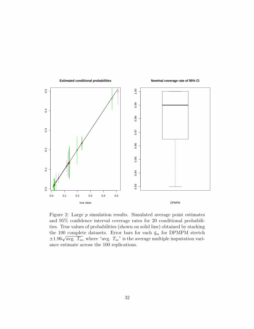
For evaluation purposes, we examine twenty arbitrary conditional probabilities, including

(i) four involving 2 variables both with missing data, (ii) four involving 2 variables with only

one having missing data, (iii) four involving 3 variables all with missing data, (iv) four

involving 3 variables with two having missing data, and (v) four involving 3 variables with

one having missing data. Figure 2 displays average point estimates and 95% confidence

interval coverage rates across the 100 simulations. The average point estimates based on

DPMPM are close to the corresponding true values, and the simulated coverage rates are at

least 93%, suggesting reasonable performance. We note that the conservative nature of the

simulated coverage rates could be an artifact of the limited number of simulation runs.

5 Imputation of TIMSS Background Variables

The TIMSS is conducted by the International Association for the Evaluation of Educational

Achievement. Data are collected on a four year cycle and made available for downloads via

a dedicated TIMSS website (www.timssandpirls.bc.edu). The goal of TIMSS is to facili-

tate comparisons of student achievement in mathematics and science across countries. In

19

addition to domain-specific test questions, TIMSS data include background information on

students including demographics, amount of educational resources at the home, time spent

on homework, and attitudes towards mathematics and science. These background variables

are all categorical.

We use data from the 2007 TIMSS that comprise 80 background variables on 90,505

students (88,129 in Grade 4 and 2,376 in Grade 5) from 22 countries. Among these 80

variables, most (68) have less than 10% missing values; six variables have between 10%

and 30% missing values; only one variable has more than 75%. Missingness rates differ by

country but not dramatically so. The TIMSS data file lists reasons for missingness, including

omitted (student should have answered but did not), not administered (missing because of

the rotation design or unintentional misprint), and not reached (incorrect responses). For

purposes of multiple imputation, we do not distinguish response reasons and treat all item

nonresponse as missing at random.

To create multiple imputations, we run DPMPMs separately in each country. Separate

imputation avoids smoothing estimates towards common values, which seems prudent since

TIMSS is intended for comparisons across countries. It is possible to extend the DPMPM

to allow borrowing information across countries using the hierarchical Dirichlet process (Si,

2012, Chapter 2). When variables are not collected in a country, we remove them from the

model for that country.

For the MCMC, we set H∗ = 20. The posterior distribution of the number of classes

among individuals (within any country) had nearly all of its mass below twenty, so that we

do not expect truncation to impact the imputations materially. Imputations with H∗ = 50

on a smaller set of countries resulted in similar performance. We also examined differ-

ent vague prior specifications for aα and bα—including, for example, (aα = 1, bα = .25),

(aα = 1, bα = 1), and (aα = 1, bα = 2)—and did not observe noticeable differences in the

posterior distributions of θ. In each country, we ran the Gibbs sampler for at least 10,000

20

iterations. MCMC diagnostics of marginal and randomly selected joint components of θ

suggest convergence. For the typical country, generating 10,000 iterations takes about 30

minutes on a standard desktop computer using a single CPU. Thus, by running the 22

countries in parallel, the entire TIMSS can be multiply-imputed within a few hours.

To assess the quality of the multiple imputations, we focus on one arbitrarily selected

country in the data file. In this country, fifty-nine variables have 10% or less missing values,

eleven variables have between 20% and 30% missing values, five variables have between 50%

and 70% missing values, and one variable has more than 80% missing values. Only 32 out

of 4,223 individuals have complete records. For purposes of evaluating the imputations, we

increased the MCMC iterations to 500,000. This took roughly 10 hours to run.

Comparisons of the marginal distributions of the observed and imputed values (Gelman

et al., 2005) show similar distributions; these are not shown here to save space. While

comforting, such diagnostics offer only partial insights into the quality of the imputations

for multivariate relationships. We therefore consider posterior predictive checks that directly

assess the ability of the imputation models to preserve associations, following the approach

in He et al. (2010) and Burgette and Reiter (2010). The basic idea is to use the imputation

model to generate not only Xmis but an entirely new full dataset, i.e., create a completed

dataset D(l) = (Xobs, X(l)mis) and a replicated dataset R(l) in which both Xobs and Xmis

are simulated from the imputation model. After repeating the process of generating pairs

(D(l), R(l)) many times (we use T = 500), we compare each R(l) with its corresponding D(l)

on statistics of interest. When the statistics are dissimilar, the diagnostic suggests that the

imputation model does not generate replicated data that look like the completed data, so

that it may not be generating plausible values for the missing data. When the statistics are

not dissimilar, the diagnostic does not offer evidence of imputation model inadequacy (with

respect to that statistic).

More formally, let S be the statistic of interest, such as a regression coefficient or joint

21

probability. Let SD(l) and SR(l) be the values of S computed with D(l) and R(l), respectively.

For each S we compute the two-sided posterior predictive probability,

ppp = (2/T ) ∗min

(T∑l=1

I(SD(l) − SR(l) > 0),T∑l=1

I(SR(l) − SD(l) > 0)

). (22)

We note that ppp is small when SD(l) and SR(l) consistently deviate from each other in one

direction, which would indicate that the imputation model is systematically distorting the

relationship captured by S. For S with small ppp, it is prudent to examine the distribution

of SR(l) − SD(l) to evaluate if the difference is practically important.

To obtain the pairs (D(l), R(l)), we add a step to the MCMC that replaces all values

of Xmis and Xobs using the parameter values at that iteration. This step is used only for

computation of the ppp; the estimation of parameters continues to be based on Xobs. When

autocorrelations among parameters are high, we recommend thinning the chain so that θ

draws are approximately independent before creating the set of R(l). Further, we advise

saving the T pairs of (D(l), R(l)), so that they can be used repeatedly with different S.

We present posterior predictive checks for 36 coefficients in a multinomial logistic re-

gression and 1,000 joint probabilities from a contingency table. The multinomial logistic

regression predicts how much students agree that they like being in school (like a lot, like a

little, dislike a little, and dislike a lot). It has 4.5% missing values. The predictor variables

include how much students agree that they have tried their best (4 categories); how much

students agree that teachers want students to do their best (4 categories); whether or not

students have had something stolen from them at school (2 categories); whether students

were hit or hurt by others at school (2 categories); whether students were made to do things

by others at school (2 categories); whether or not students were made fun of or called names

at school (2 categories); and, whether or not students were left out of activities at school (2

categories). Among all these predictors, the missing data rates range from 4.5% to 5.8%.

22

Investigations of the completed datasets indicate strong associations among the variables.

The contingency table includes whether or not students ever use a computer at home (2

categories); whether or not students ever use a computer at school (2 categories); whether

or not students ever use a computer elsewhere (2 categories); how often students use a

computer for mathematics homework (5 categories); how often students use a computer

for science homework (5 categories); and, how often students spend time playing computer

games (5 categories). Among all these variables, the missing data rates range from 10% to

63%.

We consider each coefficient and joint probability as separate S. The 1,036 values of ppp

are displayed in Figure 3. For the contingency table, only 27 out of 1,000 values are below

.05, suggesting that overall the DPMPM model generates replicated tables that look similar

to the completed ones. For the multinomial regression, three out of 36 values of ppp are below

.05 but above .01, and two are below .01. These suggest potential model mis-specification

involving the associated variables. These five low values correspond to coefficients for the two

four-category variables. These variables each have two levels with moderately low marginal

probabilities (between 5.2% and 6.8%). Apparently, the DPMPM is somewhat inaccurate

at replicating the associations with the outcome at these levels. We note, however, that the

standard errors for these coefficients are large compared to the point estimates, so that the

impact of modest imputation model mis-specification on multiple imputation inferences for

these coefficients is likely to be swamped by sampling variability.

6 Concluding Remarks

The Dirichlet process mixture of products of multinomial distributions offers a fully Bayesian,

joint model for multiple imputation of large-scale, incomplete categorical data. The approach

is flexible enough to capture complex dependencies automatically and computationally ef-

23

ficient enough to be applied in large datasets. Although based on mixture models, the

approach avoids ad hoc selection of a fixed number of classes, thereby reducing risks of using

too few classes while fully estimating uncertainty in posterior distributions.

The methods presented here have utility for multiple audiences. Organizations that

collect and disseminate large-scale categorical databases can use these imputation methods

to create completed public-use files. This places the burden of handling missing data on the

organization rather than the secondary analyst, who instead can concentrate on scientific

modeling of the multiply-imputed data. These methods also can be applied by individual

analysts to categorical data with missing values. Free software implementing the approach

in MATLAB is available from the first author, and we expect an R package to be available

on CRAN soon.

This approach can serve as the basis for additional methodological and applied devel-

opments. Many surveys include both categorical and continuous data. The nonparametric

Bayesian approach could be extended to handle mixed data, for example by letting the

continuous data be modeled as mixtures of independent normal distributions within latent

classes. Many education surveys have data with hierarchical structures, such as students

within teachers or schools within counties. The nonparametric Bayesian approach could be

extended to include random effects that account for such hierarchical structure. Finally,

many educational surveys employ multiple imputation to create “plausible values” of stu-

dents’ abilities (e.g., Mislevy et al., 1992). To the best of our knowledge, current practice

typically is to impute plausible values and missing background characteristics separately.

Doing so simultaneously may offer improved accuracy when estimating associations between

background variables and student proficiency.

24

References

Ake, C. F. (2005). Rounding after multiple imputation with non-binary categorical covariates

(paper 112-30). In Proceedings of the Thirtienth Annual SAS Users Group International

Conference, 1–11. Cary, NC: SAS Institute Inc.

Allison, P. D. (2000). Multiple imputation for missing data: A cautionary tale. Sociological

Methods and Research 28, 301–309.

Antoniak, C. E. (1974). Mixtures of Dirichlet processes with applications to nonparametric

problems. The Annals of Statistics 2, 1152–1174.

Baccini, M., Cook, S., Frangakis, C. E., Li, F., Mealli, F., Rubin, D. B., and Zell, E. R.

(2010). Multiple imputation in the anthrax vaccine research program. CHANCE 23, 1,

16–23.

Ballou, D., Sanders, W., and Wright, P. (2004). Controlling for student background in

value-added assessment of teachers. Journal of Educational and Behavioral Statistics 29,

1, 37–65.

Barnard, J. and Meng, X. L. (1999). Applications of multiple imputation in medical studies:

From AIDS to NHANES. Statistical Methods in Medical Research 8, 17–36.

Barnard, J. and Rubin, D. B. (1999). Small-sample degrees of freedom with multiple-

imputation. Biometrika 86, 948–955.

Bernaards, C. A., Belin, T. R., and Schafer, J. L. (2007). Robustness of a multivariate

normal approximation for imputation of binary incomplete data. Statistics in Medicine

26, 1368–1382.

Bishop, Y., Feinberg, S., and Holland, P. (1975). Discrete Multivariate Analysis: Theory

and Practice. MIT Press, Cambridge, MA.

25

Burgette, L. F. and Reiter, J. P. (2010). Multiple imputation via sequential regression trees.

American Journal of Epidemiology 172, 1070–1076.

Chib, S. and Hamilton, B. H. (2002). Semiparametric Bayes analysis of longitudinal data

treatment models. Journal of Econometrics 110, 67 – 89.

Dunson, D. B. and Xing, C. (2009). Nonparametric Bayes modeling of multivariate categor-

ical data. Journal of the American Statistical Association 104, 1042–1051.

Erosheva, E. A., Fienberg, S. E., and Junker, B. W. (2002). Alternative statistical models

and representations for large sparse multi-dimensional contingency tables. Annales de la

Faculte des Sciences de Toulouse 11, 4, 485–505.

Escobar, M. D. and West, M. (1998). Computing nonparametric hierarchical models. In

D. D. Dey, P. Muller, and D. Sinha, eds., Practical Nonparametric and Semiparametric

Bayesian Statistics, 1–16. Berlin: Springer-Verlag.

Ferguson, T. S. (1973). A Bayesian analysis of some nonparametric problems. The Annals

of Statistics 1, 209–230.

Ferguson, T. S. (1974). Prior distributions on spaces of probability measures. The Annals

of Statistics 2, 615–629.

Finch, W. H. (2010). Imputation methods for missing categorical questionnaire data: A

comparison of approaches. Journal of Data Science 8, 361–378.

Gebregziabher, M. and DeSantis, S. M. (2010). Latent class based multiple imputation

approach for missing categorical data. Journal of Statistical Planning and Inference 140,

3252–3262.

26

Gelman, A., Van Mechelen, I., Verbeke, G., Heitjan, D. F., and Meulders, M. (2005). Mul-

tiple imputation for model checking: Completed-data plots with missing and latent data.

Biometrics 61, 74–85.

Graham, J. W. and Schafer, J. L. (1999). On the performance of multiple imputation for

multivariate data with small sample size. In R. H. Hoyle, ed., Statistical Strategies for

Small Sample Research, 1–29. Thousand Oaks, CA: Sage.

He, Y., Zaslavsky, A. M., and Landrum, M. B. (2010). Multiple imputation in a large-scale

complex survey: a guide. Statistical Methods in Medical Research 19, 653–670.

Hirano, K. (2002). Semiparametric Bayesian inference in autoregressive panel data models.

Econometrica 70, 781–799.

Horton, N. J., Lipsitz, S. P., and Parzen, M. (2003). A potential for bias when rounding in

multiple imputation. The American Statistician 57, 229–232.

Ishwaran, H. and James, L. F. (2001). Gibbs sampling for stick-breaking priors. Journal of

the American Statistical Association 96, 161–173.

Kyung, M., Gill, J., and Casella, G. (2010). Estimation in Dirichlet random effects models.

Annals of Statistics 38, 979–1009.

Lazarsfeld, P. and Henry, N. (1968). Latent Structure Analysis. Boston: Houghton Mifflin

Co.

Li, F., Yu, Y., and Rubin, D. B. (2012). Imputing missing data by fully conditional models:

Some cautionary examples and guidelines. Tech. rep., Department of Statistical Science,

Duke University.

27

Li, K. H., Raghunathan, T. E., and Rubin, D. B. (1991). Large sample significance levels

from multiply imputed data using moment-based statistics and an f reference distribution.

Journal of the American Statistical Association 86, 1065–1073.

Little, R. J. A. and Rubin, D. B. (2002). Statistical Analysis with Missing Data: Second

Edition. New York: John Wiley & Sons.

Meng, X. L. and Rubin, D. B. (1992). Performing likelihood ratio tests with multiply-imputed

data sets. Biometrika 79, 103–111.

Mislevy, R. J., Beaton, A. E., Kaplan, B., and Sheehan, K. M. (1992). Population character-

istics from sparse matrix samples of item responses. Journal of Educational Measurement

29, 133–162.

Papaspiliopoulos, O. (2008). A note on posterior sampling from Dirichlet mixture models.

Tech. rep., Centre for Research in Statistical Methodology, University of Warwick.

Raghunathan, T. E., Lepkowski, J. M., van Hoewyk, J., and Solenberger, P. (2001). A

multivariate technique for multiply imputing missing values using a sequence of regression

models technique for multiply imputing missing values using a series of regression models.

Survey Methodology 27, 85–96.

Reiter, J. P. (2007). Small-sample degrees of freedom for multi-component significance tests

with multiple imputation for missing data. Biometrika 94, 502–508.

Reiter, J. P. and Raghunathan, T. E. (2007). The multiple adaptations of multiple imputa-

tion. Journal of the American Statistical Association 102, 1462–1471.

Rodrıguez, A. and Dunson, D. B. (2011). Nonparametric Bayesian models through probit

stick-breaking processes. Bayesian Analysis 6, 145–178.

Rubin, D. B. (1976). Inference and missing data (with discussion). Biometrika 63, 581–592.

28

Rubin, D. B. (1987). Multiple Imputation for Nonresponse in Surveys. New York: John

Wiley & Sons.

Rubin, D. B. (1996). Multiple imputation after 18+ years. Journal of the American Statistical

Association 91, 473–489.

Schafer, J. L. (1997). Analysis of Incomplete Multivariate Data. London: Chapman & Hall.

Sethuraman, J. (1994). A constructive definition of Dirichlet priors. Statistica Sinica 4,

639–650.

Si, Y. (2012). Nonparametric Bayesian Methods for Multiple Imputation of Large Scale

Incomplete Categorical Data in Panel Studies. Ph.D. thesis, Department of Statistical

Science, Duke University.

Si, Y., von Davier, M., and Xu, X. (2010). Imputation for missing data on background vari-

ables in large-scale assessment surveys. Tech. rep., Educational Testing Service, Princeton,

NJ.

Su, Y. S., Gelman, A., Hill, J., and Yajima, M. (2010). Multiple imputation with diagnostics

(mi) in R: Opening windows into the black box. Journal of Statistical Software 45, 2, 1–31.

Thomas, N. (2002). The role of secondary covariates when estimating latent trait population

distributions. Psychometrika 67, 33–48.

Van Buuren, S. and Oudshoorn, C. (1999). Flexible multivariate imputation by MICE. Tech.

rep., Leiden: TNO Preventie en Gezondheid, TNO/VGZ/PG 99.054.

Vermunt, J. K., Ginkel, J. R. V., der Ark, L. A. V., and Sijtsma, K. (2008). Multiple impu-

tation of incomplete categorical data using latent class analysis. Sociological Methodology

38, 369–397.

29

von Davier, M. (2008). A general diagnostic model applied to language testing data. British

Journal of Mathematical and Statistical Psychology 61, 287–307.

von Davier, M. (2010). Hierarchical mixtures of diagnostic models. Psychological Test and

Assessment Modeling 52, 8–28.

von Davier, M. and Sinharay, S. (2007). An importance sampling em algorithm for latent

regression models. Journal of Educational and Behavioral Statistics 32, 3, 233–251.

von Davier, M. and Sinharay, S. (2010). Stochastic approximation methods for latent re-

gression item response models. Journal of Educational and Behavioral Statistics 35, 2,

174–193.

Walker, S. G. (2007). Sampling the Dirichlet mixture models with slices. Computations in

Statistics-Simulation and Computation 36, 45–54.

Yucel, R. M., He, Y., and Zaslavsky, A. M. (2011). Gaussian-based routines to impute

categorical variables in health surveys. Statistics in Medicine 30, 29, 3447–3460.

30

−3 −2 −1 0 1 2

−3

−2

−1

01

23

Estimated regression coefficients

true value

DPMPMMICE

DPMPM MICE

0.0

0.2

0.4

0.6

0.8

1.0

Nominal coverage rate of 95% CI

Figure 1: Small p simulation results. Simulated average point estimatesand 95% confidence interval coverage rates for 45 regression coefficients.True values of coefficients (shown on solid line) obtained from a very large,complete dataset generated from the data models. Error bars for eachqm for DPMPM stretch ±1.96

√avg. Tm, where “avg. Tm” is the average

multiple imputation variance estimate across the 500 replications.

31

0.0 0.1 0.2 0.3 0.4 0.5

0.0

0.1

0.2

0.3

0.4

0.5

Estimated conditional probabilities

true value

0.9

30

.94

0.9

50

.96

0.9

70

.98

0.9

91

.00

Nominal coverage rate of 95% CI

DPMPM

Figure 2: Large p simulation results. Simulated average point estimatesand 95% confidence interval coverage rates for 20 conditional probabili-ties. True values of probabilities (shown on solid line) obtained by stackingthe 100 complete datasets. Error bars for each qm for DPMPM stretch±1.96

√avg. Tm, where “avg. Tm” is the average multiple imputation vari-

ance estimate across the 100 replications.

32

Two−sided P−values for cell counts

Fre

qu

en

cy

0.0 0.2 0.4 0.6 0.8 1.0

02

04

06

08

01

00

Two−sided P−values for coefficients

Fre

qu

en

cy

0.0 0.2 0.4 0.6 0.8 1.0

01

23

45

Figure 3: Frequency distributions of ppp for the TIMSS imputation. The leftpanel is for the 1000 cell probabilities, i.e., the completed-data counts over N ,and the right panel is for the 36 multinomial regression coefficients.

33