Nonlocal microplane model with strain-softening yield limits.pdf

International Journal of Solids and Structures 41 (2004) 7209–7240

www.elsevier.com/locate/ijsolstr

Nonlocal microplane model with strain-softening yield limits

Zden�ek P. Ba�zant a,*, Giovanni Di Luzio b,*

a McCormick School of Engineering and Applied Science, Northwestern University, CEE, 2145 Sheridan Road, Evanston,

IL 60208-3109, USAb Department of Structural Engineering, Politecnico di Milano, Piazza Leonardo da Vinci 32, 20133 Milan, Italy

Received 14 November 2002; received in revised form 26 May 2004

Available online 20 July 2004

Abstract

The paper deals with the problem of nonlocal generalization of constitutive models such as microplane model M4

for concrete, in which the yield limits, called stress–strain boundaries, are softening functions of the total strain. Such

constitutive models call for a different nonlocal generalization than those for continuum damage mechanics, in which

the total strain is reversible, or for plasticity, in which there is no memory of the initial state. In the proposed nonlocal

formulation, the softening yield limit is a function of the spatially averaged nonlocal strains rather than the local strains,

while the elastic strains are local. It is demonstrated analytically as well numerically that, with the proposed nonlocal

model, the tensile stress across the strain localization band at very large strain does soften to zero and the cracking band

retains a finite width even at very large tensile strain across the band only if one adopts an ‘‘over-nonlocal’’ general-

ization of the type proposed by Vermeer and Brinkgreve [In: Chambon, R., Desrues, J., Vardoulakis, I. (Eds.), Lo-

calisation and Bifurcation Theory for Soils and Rocks, Balkema, Rotterdam, 1994, p. 89] (and also used by Planas et al.

[Basic issue of nonlocal models: uniaxial modeling, Tecnical Report 96-jp03, Departamento de Ciencia de Materiales,

Universidad Politecnica de Madrid, Madrid, Spain, 1996], and by Str€omberg and Ristinmaa [Comput. Meth. Appl.Mech. Eng. 136 (1996) 127]). Numerical finite element studies document the avoidance of spurious mesh sensitivity and

mesh orientation bias, and demonstrate objectivity and size effect.

� 2004 Elsevier Ltd. All rights reserved.

Keywords: Microplane model; Concrete; Nonlocal continuum; Fracture; Damage; Quasibrittle materials; Softening; Numerical

methods; Finite elements

1. Introduction

Since its inception almost two decades ago (Ba�zant, 1984; Ba�zant et al., 1984), the nonlocal continuumapproach to distributed softening damage has generally been accepted as the proper way to avoid spurious

excessive localization and ensure mesh-independent energy dissipation (Ba�zant and Jir�asek, 2002). Thenonlocal models generally work well for the initial post-peak damage, which usually suffices for capturing

* Corresponding authors. Tel.: +1-847-491-4025 (Z.P. Ba�zant), Tel.: +39-022-399-4278; fax: +39-022-399-4220 (G. Di Luzio).E-mail addresses: [email protected] (Z.P. Ba�zant), [email protected] (G. Di Luzio).

0020-7683/$ - see front matter � 2004 Elsevier Ltd. All rights reserved.

doi:10.1016/j.ijsolstr.2004.05.065

mail to: [email protected]

7210 Z.P. Ba�zant, G. Di Luzio / International Journal of Solids and Structures 41 (2004) 7209–7240

the size effect on structural strength. However, unlike the nonlocal continuum damage model (Pijaudier-

Cabot and Ba�zant, 1987; Ba�zant and Pijaudier-Cabot, 1988), the plasticity-based models with softeningyield limit (initiated by Ba�zant and Lin, 1988b) are unable to simulate properly the far post-peak response(Ba�zant and Jir�asek, 2002; Jir�asek and Rolshoven, 2003; Rolshoven and Jir�asek, 2001). In particular,depending on the plasticity model formulation, it has been proven difficult to simulate the vanishing of

stress at large tensile strain across a damage band, while, for some other plasticity model, at very large

strains, the damage band was shown to localize to zero width. This is a serious problem for dynamic

behavior because the energy absorption capability of the structure with its size dependence is not captured

correctly.

To remedy this problem with nonlocal softening plasticity-based models, Vermeer and Brinkgreve

(1994), Planas et al. (1996) and Str€omberg and Ristinmaa (1996) proposed a novel formulation which wewill call ‘‘over-nonlocal’’. In their formulation, the nonlocal variable is enlarged by a factor m larger than 1,and then reduced by the ðm� 1Þ-multiple of the corresponding local variable. They demonstrated thisapproach for relatively simple tensorial constitutive models of isotropic softening-plasticity.

This study will address the problem of the far post-peak nonlocality for a damage-constitutive model of

the microplane type, and in particular for its recent powerful version for concrete called model M4 (Ba�zantet al., 2000; Caner and Ba�zant, 2000). Aside from the over-nonlocal aspect of the formulation, an alter-

native new approach to far post-peak behavior will be proposed. It will exploit the fact that, in model M4,

the strain-softening behavior is completely characterized by strain-dependent yield limits (called the stress–

strain boundaries). It will be shown that the easiest way to achieve a satisfactory far post-peak behavior,with a vanishing tensile stress across the damage band, is to make these limits functions on the nonlocal

strain instead of the local strain. This makes it possible to simulate the transition to complete fracture.

Quasibrittle materials, such as concrete, rocks, ceramics, sea ice, and fiber composites, exhibit distributed

cracking and other softening damage which needs to be described as a strain softening continuum. Already

in the mid-1970s (Ba�zant, 1976) it was recognized that the concept of softening continuum damage leads to

serious problems (Ba�zant and Jir�asek, 2002)––the boundary value problem becomes ill-posed and the

numerical calculations cease to be objective, exhibiting pathological spurious mesh sensitivity and unre-

alistic damage localization as the mesh is refined. To suppress it and to prevent the damage from localizinginto a zone of zero volume, the continuum theory must be complemented by certain conditions called

‘localization limiters’, involving a characteristic length of the material (Ba�zant, 1976; Ba�zant and Oh, 1983;Ba�zant et al., 1984; Ba�zant and Belytschko, 1985).As the simplest localization limiter, one may adjust the post-peak slope of the stress–strain diagram as a

function of the element size. This is done in the crack band model (Ba�zant, 1976; Ba�zant and Oh, 1983),which is the model most widely used in practice and adopted in commercial codes (DIANA, ATENA,

SBETA, etc.). Another popular regularizing technique uses a second-order gradient model (Aifantis, 1984;

Zbib and Aifantis, 1988; Lasry and Belytschko, 1988; M€uhlhaus and Aifantis, 1991; de Borst andM€uhlhaus, 1992a,b; Vardoulakis and Aifantis, 1991; Pamin, 1994). Recently, an effective modification ofthe gradient approach has been developed by Peerlings et al. (1996). A different gradient-type regularization

model is based on the concept of Cosserat continuum (Cosserat and Cosserat, 1909), which is able to limit

localization in a shear band but not in tension (M€uhlhaus and Vardoulakis, 1987; de Borst, 1991; Stein-mann and Willam, 1992). A simple regularization technique, which works only for a limited range of

loading rates, is the viscoplastic regularization, in which some artificial strain-rate dependent terms are

inserted into the constitutive law (Needleman, 1988; Loret and Prevost, 1990).

A broad class of localization limiters is based on the concept of a nonlocal continuum, which is used inthis work. The nonlocal concept was introduced in the 1960s (Eringen, 1966; Kr€oner, 1968; etc.) for elasticdeformations and later expanded to hardening plasticity. In a nonlocal continuum, the stress at a certain

point depends not only on the strain at that point itself but also on the strain field in the neighborhood of

that point. Ba�zant (1984) and Ba�zant et al. (1984) introduced the nonlocal concept as a localization limiter

Z.P. Ba�zant, G. Di Luzio / International Journal of Solids and Structures 41 (2004) 7209–7240 7211

for a strain-softening material. This formulation was soon improved in the form of the nonlocal damage

theory (Pijaudier-Cabot and Ba�zant, 1987; Ba�zant and Pijaudier-Cabot, 1988), nonlocal plasticity with asoftening yield limit (Ba�zant and Lin, 1989) and nonlocal smeared cracking (Ba�zant and Lin, 1988b), andwas demonstrated in practical problems (Ba�zant and Lin, 1988a, 1989; Saouridis and Mazars, 1992).The governing parameter in the nonlocal continuum is the material characteristic length l depending on

the size of the neighborhood over which the strain or some other variable is averaged. When l is equal to orless than the element size, the nonlocal formulation reduces to a local formulation. The characteristic length

has a major influence on the softening behavior of structure. In the early studies, this length was assumed to

be correlated to the maximum aggregate size da, l ¼ 3da (Ba�zant and Oh, 1983). However, it is now ac-

cepted that the characteristic length l is also influenced by other parameters (especially Irwin’s charac-teristic size of the fracture process zone). Experience shows that the optimum value of l can change

significantly from one type of problem to another, which could be explained by the fact that the directionaldependence of microcrack interactions (Ba�zant, 1994; O�zbolt and Ba�zant, 1996) is ignored.Classically, the nonlocal approach has been applied to the standard constitutive models expressed in

terms of the stress and strain tensors and their invariants. During the last decade, the earlier nonlocal

approach has been introduced into an early version of the microplane model (Ba�zant and O�zbolt, 1990;O�zbolt and Ba�zant, 1996), in which the constitutive behavior is characterized in terms of stress and strainvectors acting on arbitrarily oriented planes in the material (Ba�zant, 1984; Ba�zant and Oh, 1985). Theobjective of this paper is to combine the microplane model with the recently improved nonlocal approach

that leads to a correct localization behavior, and demonstrate it for a recent version of microplane modelemploying the concept of softening stress–strain boundaries. Although the main advantage of microplane

model lies in the simulation of damage for complex compressive triaxial stress histories, the comparisons

with experiments will have to focus on tensile fracture because there are hardly any test data on damage

localization for such histories.

2. Review of microplane model

The microplane constitutive model is defined by a relation between the stresses and strains acting on a

plane in the material called the microplane, having an arbitrary orientation (characterized by its unit

normal ni). The basic hypothesis, which enhances stability of post-peak strain softening (Ba�zant, 1984), isthe kinematic constraint, consisting in the fact that the strain vector �N

! on the microplane (Fig. 1a) is the

projection of the strain tensor �, i.e., �Ni ¼ �ijnj. The normal strain on the microplane is �N ¼ ni�Ni, that is,

Fig. 1.

hemisp

�N ¼ Nij�ij; ð1Þ

(a) Strain components on general microplane; (b) directions of microplane normals (circles) for system of 21 microplanes per

here; (c) directions of microplane normals (circles) for system of 28 microplanes per hemisphere.


where Nij ¼ ninj (and the repetition of the subscripts, referring to Cartesian coordinates xi, implies sum-mation over i ¼ 1; 2; 3). The shear strains on each microplane are characterized by their components inchosen directions M and L given by orthogonal unit coordinate vectors ~m and~l, of components mi, li, lyingwithin the microplane. The unit coordinate ~m is chosen and ~l is obtained as ~l ¼ ~m�~n. To minimizedirectional bias, vectors ~m are alternatively chosen normal to axes x1, x2, or x3. The shear strain componentsin the directions of ~m and~l are �M ¼ mið�ijnjÞ and �L ¼ lið�ijnjÞ, and by virtue of the symmetry of tensor �ij,

�M ¼ Mij�ij; �L ¼ Lij�ij; ð2Þ

in which Mij ¼ ðminj þ mjniÞ=2 and Lij ¼ ðlinj þ ljniÞ=2 (Ba�zant and Prat, 1988).Because of the kinematic constraint relating the strains on the microlevel (microplane) and macrolevel

(continuum), the static equivalence (or equilibrium) of stresses between the macro- and microlevels is ex-pressed by the principle of virtual work (Ba�zant, 1984), written for the surface X of a unit hemisphere:

2p3

rijd�ij ¼Z

XðrNd�N þ rLd�L þ rMd�MÞdX: ð3Þ

This equation means that the virtual work of macrostresses (continuum stresses) within a unit sphere must

be equal to the virtual work of microstresses (microplane stress components) regarded as the tractions on

the surface of a sphere (for a detailed physical justification, see Ba�zant et al., 1996a). The integral physicallyrepresents a homogenization of different contributions coming from planes of various orientations withinthe material. Substituting d�N ¼ Nijd�ij, d�L ¼ Lijd�ij and d�M ¼ Mijd�ij, and noting that the last variationalequation must hold for any variation d�ij, one gets the following basic equilibrium relation (Ba�zant, 1984):

rij ¼3

2p

ZXsij dX ¼ 6

XNm

l¼1wls

ðlÞij with sij ¼ rNNij þ rLLij þ rMMij: ð4Þ

The numerical integration, indicated above, is best done according to an optimal Gaussian integration

formula for a spherical surface (Stroud, 1971; Ba�zant and Oh, 1986) representing a weighted sum over the

microplanes of orientations ~nl, with weights wl normalized so thatPNm

l¼1 wl ¼ 1=2 (Ba�zant and Oh, 1985,1986). An efficient formula that still yields acceptable accuracy involves 21 microplanes (Ba�zant and Oh,1986; Fig. 1b); in this work the Stroud’s formula with 28 microplanes has been used (Fig. 1c). In finite

element programs, integral (4) must be evaluated at each integration point of each finite element in each

time step. The values of N ðlÞij , MðlÞij and LðlÞij for all the microplanes l ¼ 1; . . . ;N are common to all inte-

gration points of all finite elements, and are calculated and stored in advance.The most general constitutive relation on the microplane level may give rN , rL and rM as functionals of

the histories of �N , �M , �L. But normally it is suffices to consider that each of rN , rL and rM depends only on

its current corresponding strain �N , �M , �L because cross dependencies on the macrolevel, such as sheardilatancy, are automatically captured by interaction among microplanes of various orientations. An

exception is the frictional yield condition relating the normal and the shear components on the microplane

with no strain dependence.

In microplane model M4 (as well as M3, Ba�zant et al., 1996a,b and M5, Ba�zant and Caner, 2002), theconstitutive relation in each microplane is defined by (1) incremental elastic relation and (2) stress–strainboundaries (softening yield limits) that cannot be exceeded. The normal components are split into their

normal and deviatoric parts, i.e. rN ¼ rV þ rD, �N ¼ �V þ �D, and then the incremental elastic relations arewritten as

drV ¼ EV d�V ; drD ¼ EDd�D; drM ¼ ETd�M ; drL ¼ ETd�L; ð5Þ

where EV , ED and ET are the microplane elastic moduli which are always positive and, in the case of virginloading, are constant and expressed in terms of Young’s modulus E (macroscopic) and Poisson’s ratio m;


EV ¼ E=ð1� 2mÞ, ED ¼ 5E=½ð1þ mÞð2þ 3gÞ and ET ¼ gED. The value g ¼ 1 is, for various reasons, optimal(Ba�zant and Prat, 1988; Carol and Ba�zant, 1997). For unloading and reloading, EV , ED and ET are functions

of the current strain and the maximum strain reached so far. The stress–strain boundaries, which may be

regarded as strain dependent yield limits, consist of the following conditions:

rN 6 FN ð�N Þ; F �V ð�V Þ6 rV 6 F þV ð�V Þ; F �D ð�DÞ6 rD 6 F þD ð�DÞ;jrM j6 FT ðrN ; �V ; �I ; �IIIÞ; jrLj6 FT ðrN ; �V ; �I ; �IIIÞ;

ð6Þ

Except for the last two conditions, which model friction, interactions among various components need not

be considered, since the cross effects are adequately captured by interactions among various microplane due

to the kinematic constraint. The unloading conditions are formulated separately for each microplanecomponent. Unloading occurs when the incremental work of a microplane component becomes negative,

i.e. when, separately for each component:

rND�N 6 0; rV D�V 6 0; rDD�D 6 0; rMD�M 6 0; rLD�L 6 0: ð7Þ
Reloading for any component occurs when the corresponding condition among the foregoing is violated
while the corresponding condition (6) is a strict inequality. The expressions for the boundary functions,

identified for model M4 by fitting the available test data, are given in Appendix A.

3. Basic concept of nonlocal model

The nonlocal model, in general, consists in replacing a certain local variable f ðxÞ, characterizing thesoftening damage of material, by its nonlocal counterpart �f ðxÞ. The nonlocal operator is defined as

�f ðxÞ ¼ZV

aðx; nÞf ðnÞdV ðnÞ; ð8Þ

where V is the volume of the structure, x, n are the coordinates vectors, and aðx; nÞ is the normalizednonlocal weight function:

aðx; nÞ ¼ aðx� nÞRV aðx� fÞdV ðfÞ : ð9Þ

Here aðx� nÞ is the basic nonlocal weight function for an unbounded medium;RV aðx� fÞdV ðfÞ is a

constant if the unrestricted averaging domain does not tend to protrude outside the boundaries. The weight

function aðx� nÞ is often taken as a bell-shaped function. Its analytical expression, used in this work, is:

aðx; nÞ ¼ ð1� jx� nj2=R2Þ2 if 06 jx� nj6R;0 if R6 jx� nj;

�ð10Þ

where R is a parameter proportional to the material characteristic length l (Fig. 2 for one- and bi-

dimensional case), R ¼ q0l. Note that jx� nj ¼ffiffiffiffiffiffiffiffiffiffiffiffiffiffiffiffiffiffiffiðxi � niÞ2

qand aðx; xÞ ¼ 1. The coefficient q0 is determined

so that the volume under function a be equal to the volume of the uniform distribution

(q0 ¼ 15=16 ¼ 0:9375 for 1D, q0 ¼ffiffiffiffiffiffiffiffi3=43

p¼ 0:9086 for 2D, q0 ¼

ffiffiffiffiffi353p

=4 ¼ 0:8178 for 3D).The averaging function (10) is doubtless a simplification. Properly, a should also depend on the ori-

entation of the principal stress axes at n and x, as proposed by Ba�zant (1994) on the basis of microme-chanics analysis of a random system of interacting and growing microcracks. A combination of that kind of

nonlocal continuum with the microplane model was implemented by O�zbolt and Ba�zant (1996), and al-lowed an improved representation of opening and shear fractures with the same material model (Ba�zantand O�zbolt, 1990). However, the implementation is more complicated and is not needed for the presentpurpose.

Fig. 2. Normalized nonlocal bell-shaped weight function: (a) in one-dimension, (b) in two-dimension.


Vermeer and Brinkgreve (1994), Str€omberg and Ristinmaa (1996), and Planas et al. (1996) (see alsoBa�zant and Planas, 1998), introduced a refinement of the standard nonlocal formulation, here called over-nonlocal, in which the averaged nonlocal variable �f ðxÞ is replaced by the following over-nonlocal variable:

Fig. 3.

profile

f ðxÞ ¼ m�f ðxÞ þ ð1� mÞf ðxÞ ð11Þ

(a) Linear softening; (b) rectangular weight function; (c) strain profiles in the localization band for various values of m; (d) strains in the localization band for m � 1.

(d)

0.0 1.0 2.0 3.0 4.0 5.00.0

1.0

2.0

3.0

m=0.9m=1

m=1.2

displacement x 10-5[m]

stre

ss [M

Pa]

(c)

0.000 0.025 0.050 0.075 0.1000.0000

0.0040

0.0080

0.0120

m = 0.9

coordinate

stra

in

(a)

0.000 0.025 0.050 0.075 0.1000.0000

0.0004

0.0008

0.0012

0.0016

0.0020

m = 1.2

coordinate

stra

in

(b)

0.000 0.025 0.050 0.075 0.1000.0000

0.0040

0.0080

0.0120

m = 1

coordinate

stra

in

Fig. 4. Strain-softening bar: (a) strain profile along the bar for m ¼ 1:2; (b) strain profile along the bar for m ¼ 1; (c) strain profile alongthe bar for m ¼ 0:9; (d) stress–displacement curves for different values of m.


in which x is the nonlocal variable obtained from Eq. (8), and m is an empirical coefficient. Str€omberg andRistinmaa (1996) called it the ‘mixed local and nonlocal model’. Planas et al. (1996) called this formulation a

‘nonlocal model of the second kind’. The results of both confirmed the spurious localization to be avoidedeven at large strains if m > 1. Planas et al. (1996) rigorously proved, for a uniaxial stress field, that the

localization zone is finite if and only if m > 1. It was also proven (Ba�zant and Planas, 1998) that, for thespecial case of uniaxial stress, the formulation with m > 1 is equivalent, in terms of strain rate distribution at

bifurcation from a uniform strain state, to the nonlocal damage model of Pijaudier-Cabot and Ba�zant (1987).

4. Nonlocal generalization of microplane model

The original nonlocal model of Ba�zant (1984) and Ba�zant et al. (1984) led to spurious zero-energyinstability modes (Ba�zant and Cedolin, 1991), which had to be suppressed by an artificial elastic restrain, at


the cost of making softening to zero stress unattainable. These difficulties can be traced to the nonlocality of

the incremental elastic strains. On the other hand, according to the later findings of Pijaudier-Cabot and

Ba�zant (1987) and Ba�zant and Pijaudier-Cabot (1988), the nonlocality of inelastic strain is free of thisundesirable side effect.The microplane model differs from the classical tensorial model of plasticity and continuum damage by

the fact that the stress–strain boundaries, which define the inelastic strain, depend on the total strain only.

This suggests a nonlocal generalization in which the stress–strain boundaries are evaluated from the

nonlocal total strains (instead of being evaluated from the local total strain, with the nonlocal averaging

postponed until after the inelastic strains have been evaluated).

Based on these considerations, a proposal is here made for a new kind of nonlocal formulation in which

the elastic stress increments are local and the boundaries in Eq. (6) are modified as follows:

stra

in

(a)

Fig. 5.

proble

rN 6 FN ð�N Þ; rV 6 F þV ð�V Þ; F �D ð�DÞ6 rD 6 F þD ð�DÞ;jrM j6 FT ðrN ; �V ; �I ; �IIIÞ; jrLj6 FT ðrN ; �V ; �I ; �IIIÞ:

ð12Þ

For the sake of generality, the arguments in these conditions are considered as over-nonlocal;

�V ¼ �kk=3; �N ¼ Nij�ij; �D ¼ �N � �V ; �M ¼ Mij�ij; �L ¼ Lij�ij; ð13Þ

where �ij ¼ m��ij � ðm� 1Þ�ij, �ij are the Cartesian components of �, and the over-bar denotes the nonlocalcounterpart of the variable as defined in Eq. (8). The standard nonlocality is the special case for m ¼ 1.Considering a state of uniaxial tension, r, in the direction normal to a localization band, we can easily

explore the basic properties of the model. The proposed nonlocal formulation is analyzed for the case of a

uniaxial stress–strain relation of the form:

for x 2F : r ¼ f ½��ðxÞ else : r ¼ E�ðxÞ: ð14Þ

Stress r is assumed to be uniform, F is the localization band of softening material, and f is a mono-

tonically decreasing function approaching 0 for ��!1. Let us check whether the displacement profile �ðxÞcould have the following expression:

L = 12 cmA = 9 cm2

n = 4, 12, 24, 48

L

F=σAF=σA

1 2 …. n

L

F=σAF=σA

1 2 …. n

L

F=σAF=σA

L δ

F=σAF=σA

1 2 …. n

0.00 0.04 0.08 0.12

0.00

0.0004

0.0008

0.0012

0.0016

0.002

12 Elements

4 Elements

24 Elements48 Elements

12 Elements

4 Elements


4 Elements


coordinate [m](b)

(a) Longitudinal strain along the bar for various degrees of mesh refinement; (b) Geometry description for the one dimensional

m.

(a

(c

Fig. 6.

local m


�ðxÞ ¼ rEþ �FðxÞ; ð15Þ

where �FðxÞ is the unknown strain profile in the localization bandF. For the sake of simplicity, we assume,

in F, a linear softening function, and for the weight function a the rectangular function (Fig. 3b).Considering the over-nonlocal refinement and the linear softening function (Fig. 3a), we can rewrite Eq.

(14) as

for x 2F : r ¼ r0 � Hðm��ðxÞ þ ð1� mÞ�ðxÞ � �0Þ: ð16Þ

Averaging the strain in Eq. (15), the nonlocal strain ��ðxÞ in Eq. (16) has, according to Eq. (8), the followingexpression:

)

σ[M

pa]

ε (strain)0.000 0.004 0.008 0.012 0.016 0.020

0.00

1.00

2.00

3.00

δ0.0 0.04 0.08 0.12 0.16

0.0

500.0

1000.0

1500.0

2000.0

2500.0

12 Elements

4 Elements


12 Elements

4 Elements


4 Elements


displacement [mm]

For

ceF

[N]

(b)

δ0.0 0.04 0.08 0.12

0.0

500.0

1000.0

1500.0

2000.0

2500.0

displacement [mm]

For

ceF

[N]

12 Elements

4 Elements


12 Elements

4 Elements


4 Elements


)

δ0.0 0.03 0.06 0.09 0.12

0.0

500.0

1000.0

1500.0

2000.0

2500.0

displacement [mm]

For

ceF

[N]

(d)

12 Elements

4 Elements


12 Elements

4 Elements


4 Elements


Load–displacement curves for various degrees of mesh refinement: (a) local stress–strain law; (b) nonlocal microplane model; (c)

icroplane model; (d) nonlocal microplane model obtained through the averaging of the inelastic strain (Appendix B).

Mesh of 30 elements Mesh of 120 elements

P

P

P

P

P

P

P

P

d = 8 cmh = 20 cmb = 3.5 cmd

h

d/6 d/6

0.0 0.1 0.20.0

1000.0

2000.0

3000.0

4000.0

dislacement δ [mm]

forc

eP

/2[N

]

(d)

0.0 0.1 0.2 0.30.0

1000.0

2000.0

3000.0

4000.0

dislacement δ [mm]

30 elements

120 elements

forc

eP

/2[N

]

(e)

(a) (b) (c)

30 elements

120 elements

Fig. 7. (a) Geometry of the rectangular panel; (b) mesh with 30 finite elements; (c) mesh with 120 finite elements. Load–displacement

curves for the two different refined meshes: (d) local microplane model (e) nonlocal microplane model.


��ðxÞ ¼ 1l

lrE

þZV�FðnÞaðn� xÞdn

; ð17Þ

where, for a very long bar (extending from �1 to þ1), l ¼Rþ1�1 aðn� xÞdn ¼ constant. Since Eq. (17) is

defined in the localization bandF, and �FðxÞ ¼ 0 for x 62F, we can evaluate the integral in Eq. (17) from�h=2 to h=2, where h is the length of localization zone. Substituting Eq. (17) into Eq. (16), we obtain:

B ¼ ml

Z h=2

�h=2�FðnÞaðn� xÞdnþ ð1� mÞ�FðxÞ; ð18Þ


where B ¼ �0 � ðr� r0Þ=H � r=E is a constant for a given uniaxial tension r. Eq. (18) is a Fredholmintegral equation of the second kind. For the sake of simplicity, Eq. (18) is solved numerically for a fixed

value of h chosen as h ¼ 0:8l. The bar is discretized into equal elements of constant �F. The integral isevaluated using a single integration point in the center of each element. The resulting linear system is solvedfor different values of m.Fig. 3 shows the strain profiles, for different values of m. When the standard nonlocal model (m � 1) is

considered, the strain distribution has the form of Dirac’s d-function (Fig. 3d). The total elongation of thebar can be considered as the sum of the elastic part, proportional to the bar length, and the inelastic part,

independent of the bar length (as shown by Planas et al., 1993). Thus, this formulation (m � 1) is equivalentto a cohesive crack model. For m < 1, the strain distribution along the bar has an unrealistic shape: at the

midlength of the localization zone, the value of the strain is less than its value at the boundaries, between

the localization band and the rest of the bar, where there is no continuity of the strain profile (Fig. 3c). Onthe other hand, using m > 1, the strain profile is realistic: (1) it reaches the maximum value at the midlength

of the localization band; (2) the strain is continuous at the boundaries, between the localization zone and

the rest of the bar, where the inelastic strain continuously approaches the elastic one (Fig. 3c). A more

rigorous and complete study, presented in Planas et al. (1996) and also in Ba�zant and Planas (1998, Chapter13), which treats the length of the localization zone, h, as unknown in Eq. (18), shows that h is finite if andonly if m > 1. It needs to be noted, however, that the present analysis with fixed h leads to an admissiblesolution for only one specific value of m, and so the profiles for other values of m do not represent actual

Fig. 8. Discretization meshes, geometry and load–deflection curves for the tensile test with uniform (a) and concentrated (b) dis-

placement control.


admissible solutions. The actual solutions for other m would be characterized by other values of h anddifferent profiles.

The behavior at very large strain, �!1, across the localization band also be easily clarified. Notingthat ��ðxÞ ¼ 1

l

RV �ðr þ xÞaðrÞdr ¼ 1

l

RF�ðr þ xÞaðrÞdr þ

RE

rE aðrÞdr

� �, where V ¼F [ E, and taking into

account Eq. (14), we must have, for x 2F,

frEl

ZE

aðrÞdr

þ 1l

ZF

aðrÞ�ðxþ rÞdr¼ r; ð19Þ

where lim f ð�Þ ¼ 0 for �!1. Now, if we assume that r! 0 and �!1, this expression becomes

f ð0þ1Þ ¼ 0 ¼ r, and so this condition is satisfied. On the other hand, if we assume that r! rr > 0 at

�!1, the left-hand side in Eq. (19) is f ðconstant þ1Þ ! 0, which cannot be equal to the right-hand side

if the residual stress r is finite. Hence, the residual stress across the band must vanish at very large dis-

placement. This is not true for the classical nonlocal model with averaging of inelastic strain as shownnumerically by Jir�asek (1998).The foregoing favorable properties of the nonlocal model are gained by making only the softening

microplane stress–strain boundaries (strain-softening yield limits) function of the nonlocal strain. It is

crucial to recognize that the elastic strains on the microplane (as well as any hardening inelastic strains)

must depend only on the local strain, or else one would engender zero energy instability modes (such modes

plagued the original nonlocal strain-softening continuum model, the so called imbricate model, and had to

Fig. 9. Crack propagation for two different tensile tests. Left: for the concentred load. Right: for the distributed load.


be suppressed by parallel elastic coupling, which precluded the strain-softening from terminating with zero

stress). This means that, in every constitutive law in which the softening depends on the strains, objectivity

can be reached by making the softening function dependent on the nonlocal strains.

0 0.02 0.04 0.06 0.08 0.1

0

0.01

0.02

0.03

0.04

0.05

0.06

0.07

dd

P/4P/4

0 0.05 0.1 0.15 0.2

0

0.05

0.1

0.15

2d2d

P/4P/4

0 0.05 0.1 0.15 0.2 0.25 0.3 0.35 0.4

0

0.05

0.1

0.15

0.2

0.25

0.3

P/4P/4

4d4d

00.020.040.060.080.1

0

0.02

0.04

0

0.02

0.04

0.06

0.08

0.1

2384d

1282d

64d

n. elementssize

2384d

1282d

64d

n. elementssize

d/6

d/12

d/6

d/12

P

2.5 d

d

b

P

2.5 d

d

PPP

2.5 d2.5 d

dd

bb

d = 7,62 cm; b = 3,81 cm

Fig. 10. Three-point bending (test of Ba�zant and Pfeiffer, 1987): geometry description, and meshes used for three different beam sizes.

Fig. 11. Three-point bending (test of Ba�zant and Pfeiffer, 1987): comparison of test data and optimum fit of data by size effect law for

three-point bending of Fig. 10: (a) linear regression plot; (b) Ba�zant’s size effect law; (c) load–deflection curves for the three differentsizes; (d) deformed specimen.


As an example, a one-dimensional strain-softening bar (with cross section area 4 cm2 and length 10 cm)

is numerically simulated for different values of m. The nonlocal generalization of microplane model M4 isused, with l ¼ 7:62 cm. This numerical example confirms what was observed in the previous simplifiedmodel––only if the over-nonlocal formulation is used, a realistic description of the fracturing process isachieved. Fig. 4 shows that the fracturing strain is localized into a finite length, independently of the

number of elements, only if m is larger than 1 (Fig. 4a). On the other hand, if the classical nonlocal model

ðm ¼ 1Þ is adopted, the fracturing strain tends to localize into one element (Fig. 4b) even if the globalresponse is correct (i.e., objective) in terms of the stress–displacement curve (Fig. 4d). Using a value of mless than 1 (i.e. m ¼ 0:9), regularization is not achieved: the strain localizes into one element (Fig. 4c). Fig.4d shows that, for m ¼ 0:9, the stress–displacement curve shows a very steep post-peak branch approaching


a snap-back. The slope of the load–displacement diagram could be adjusted by changing the softening

parameters, and so one cannot say that m ¼ 1 gives a correct global response and m ¼ 0:9 does not.The reason why the classical continuum with the averaging of inelastic strains (or inelastic stresses) does

not have the desired localization properties is that the inelastic strains (or inelastic stresses) in the modelsused are not functions of the nonlocal total strains. In this kind of models, no so much improvement was

found. After adding a certain artificial feature, which makes m variable, satisfactory behavior can be

achieved (see Appendix B).

5. Numerical studies

Without a nonlocal formulation (and without the use of the crack band model), the finite-element codeswith strain softening exhibit unacceptable spurious mesh sensitivity. Especially, they cannot capture the size

effect and crack propagation direction at a small angle with respect to the mesh line (directional bias of the

mesh). To demonstrate that the present nonlocal formulation is free of these problems, seven examples of

finite elements analysis using the over-nonlocal formulation with nonlocal stress–strain boundaries are

presented. Monotonic loads and small strains and rotations are assumed. In examples number 1, 2 and 4,

three-dimensional 8-node brick elements and implicit equilibrium solutions are used, while in the remaining

examples a plane-strain analysis with explicit time integration is performed (the details of the numerical

algorithm can be found in Appendix C).

1. One dimensional bar. Consider a straight bar of length L and a constant cross section of area A subjected

to uniaxial tension (Fig. 5a). The material parameters are l ¼ 7:62 cm, m ¼ 1:5 and E¼ 27,500 MPa. The

Fig. 12. Three-point bending example for testing the directional bias of mesh: geometry, meshes discretization, and load–displacement

curve.


bar is loaded by a displacement applied at one end. To fix the place of damage, one quarter of the bar

adjacent to the opposite end is assigned a Young’s modulus 7.5% smaller than the rest. When the stress

reaches the tensile strength limit, the softening starts in the weak element and, in a local formulation, all

the other elements undergo elastical unloading. The nonlocal formulation of microplane model is able toprevent the localization of softening into one element. The strain distributions along the bar for various

degrees of mesh refinement (4, 12, 24, 48 elements) are shown in Fig. 5b, and the load displacement

curves are plotted in Fig. 6.

2. Direct tensile test. The rectangular panel in Fig. 7a, the same as considered by Ba�zant and O�zbolt (1990),is loaded in tension. The material parameters are l ¼ 7:62 cm, m ¼ 1:5 and E¼ 27,500 MPa. Because ofsymmetry, only one-quarter of the specimen is modeled. To fix the place of localization, a weak element,

Fig. 13. Three-point bending example for testing the directional bias of mesh: crack distribution for the regular mesh (left) and for the

slanted mesh (right) at different loading levels.


shown darker in Fig. 7, is introduced by reducing the elastic modulus by 7.5%. To show that the results

are not mesh-sensitive, two finite element meshes are used: one with 30 (Fig. 7b) and the other one with

120 (Fig. 7c) finite elements. Fig. 7d and e shows the load–displacement curves for both meshes with

local and nonlocal microplane model.3. Notched tensile test. The test is described in Fig. 8. The Young’s modulus of loading plates is 10-times

higher than that of concrete. At the vertical edges, two types of displacement control are considered: a

uniform displacement (non-rotating plates) and a point displacement (rotating plates), as shown in Fig.

8. The material parameters l ¼ 3:81 cm, m ¼ 1:5 and E¼ 27,500 MPa. Fig. 8 shows the load–displace-ment curves for both cases. The reader can clearly see, that the curves tend to zero when the displace-

ments become large enough. In Fig. 9 one can see the crack distribution at different load levels, on

the left side for rotating platens (realistic fracture propagation) and on the right side for non-rotating

platens (the displacement being almost uniform across the ligament).4. Size effect in three-point bending. One important consequence of nonlocality is the size effect. The three-

point-bending tests of Ba�zant and Pfeiffer (1987) are considered. Fig. 10 shows the geometry, similar foreach size, and the finite element meshes for three different specimen sizes, with size ratio 1:2:4. The small-

est specimen depth is d ¼ 7:62 cm. The thickness is b ¼ 3:81 cm, for each size. The characteristic length istaken as l ¼ 3:175 cm, and m ¼ 1:2. The tensile strength of concrete and the elastic modulus are assumedas f 0t ¼ 2:8 MPa and E¼ 27,500 MPa. The nominal stress at failure is defined as rN ¼ Pmax=db, wherePmax is the maximum load. Comparison with the test data is shown in Fig. 11. The curves in Fig. 11 rep-

resent a good fit of the present nonlocal model to the test results smoothed by Ba�zant’s size effect law(Ba�zant, 1984; Ba�zant and Pfeiffer, 1987; RILEM Committee QFS, 2004):

Fig. 14. T

slanted m

rN ¼Bf 0tffiffiffiffiffiffiffiffiffiffiffiffiffiffiffiffiffiffiffiffi

1þ D=D0

p ; ð20Þ

in which constants B and D0 haven been determined from the test data (for the most general derivation

from dimentional analysis and asymptotic matching, see Ba�zant, 2004). The average measured maximumloads for the three specimen sizes are 3105, 4635 and 7784 N, while those obtained from the present

nonlocal model are 3260, 4876 and 8052 N, respectively, the errors being 4.9%, 5.2% and 3.4%.

hree-point bending example for testing the directional bias of mesh: crack distribution for the regular mesh (left) and for the

esh (right) at different loading levels for the local microplane model M4.

Fig. 15. Single-edge-notched beam subject to antisymmetric four-point shear loading: geometry, mesh discretization, and crack

propagation for the four point shear (based on maximum principal strain).


5. Elimination of directional mesh bias. As mentioned before, the crack band model is not able to simulate a

fracture propagation direction at small angle with the mesh line. This problem is studied using the speci-

men geometry, boundary condition and the meshes shown in Fig. 12. The lines of the slanted mesh are

inclined by about 23�. Fig. 12 presents the load–displacement curves for both cases, for material param-eters l ¼ 2:54 cm and E¼ 27,500 MPa. One can see that both meshes give practically the same load–dis-placement curves, and the same is true for fracture propagation at different load levels (Fig. 13). Using a

δ [mm]

P [KN]Experimental (44.1 kN)

AA

25 cm

24 mm

12 cm

24 cm

24 mm

12 mm

24 cm

(a) (b)

0.0 0.1 0.2 0.3 0.4

0

10

20

30

40

50

Fig. 16. Concrete cone pull-out of headed stud: (a) geometry description; (b) load–displacement curve compared with the maximum

experimental load.


local microplane M4 with no regularization, the numerical solution exhibits a strong mesh bias for thefracture propagation (Fig. 14).

Antisymmetric four-point-shear. To show how the model is also able to predict a crack with a curved

path, a notched specimen, subjected to an antisymmetric four-point shear loading, is considered (Fig. 15,

a test used by Schlangen, 1993). The thickness of the beam is 38 mm. A mesh of 864 triangular 3-node

elements is used (Fig. 15). The material parameters are l ¼ 1:905 cm, m ¼ 1:25 and E¼ 27,500 MPa.When the antisymmetric load is applied, a crack starts from the left corner of the notch and grows

upwards to the left side of the loading platen. A second damage zone develops from the top surface of

the specimen. Fig. 15 illustrates the crack propagation and cracking distribution at subsequent loadingstages. Note that the experimentally observed curved crack path (Schlangen, 1993) is qualitatively

reproduced, even if the second damage zone keeps growing for large displacement (this is due to the

effect of the boundary conditions).

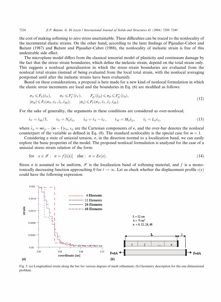
6. Concrete cone pull-out of headed stud. The case of headed anchor subjected to a tensile load is considered

(UE Anchor Project, 2001). Many experimental data and some numerical studies have shown how the

headed stud is able to transfer considerable tensile load without any reinforcement and demonstrated

that the failure mechanism is a cone shaped fracture. Simulation of this problem by the cohesive crack

model is difficult, not only because the crack path is not known a priori but also because a tensile frac-ture model is insufficient. The failure mode is not of a pure mode I type and a general triaxial constitutive

law is necessary to reproduce correctly the entire response history. The proposed over-nonlocal micro-

plane model is used to simulate the ultimate loads measured in pull-out test of a cast-in situ anchor, with

bar diameter 12 mm, embedment length equal hef ¼ 65 mm, and head (stud) diameter 24 mm (see Fig.

16). The assessment of the parameters of the constitutive models is done by fitting the available mechan-

ical properties of the concrete obtained from independent tests: compressive strength f 0c ¼ 30:8 MPa,tensile strength f 0t ¼ 2:86 MPa, Young modulus Ec ¼ 35 GPa, and fracture energy GF ¼ 64:5 N/m,which gives l ¼ 3:6 cm. Furthermore, m ¼ 1:25. The steel bar is considered to be linearly elastic, withYoung’s modulus Es ¼ 210 MPa and Poisson’s ratio ms ¼ 0:3. This assumption is justified by the fact that

Fig. 17. Concrete cone pull-out of headed stud: evolution of the maximum principal strain for different values of the stud displacement.


the measured ultimate load Nu ¼ 44:1 kN leads to a stress in the steel rod (Nu=ð0:25p/2s Þ ¼ 389:9 MPa)

lower than the yielding strength. For numerical simulations by the microplane model, an axi-symmetric

mesh of CST finite elements is used and the diameter of the concrete block is 25 cm. The mesh is

constrained in the direction of the applied load, with sliding supports located at a distance of 23 cm fromthe axis of the stud. Fig. 16b compares the over-nonlocal simulation with the measured ultimate load.

The numerical prediction (43.7 kN) is about 1.0% smaller than the experimental data (44.1 kN). Fig.

17 further shows the contours of the maximum principal strain computed by the microplane model at

different values of the load-point displacement. As one can see, the strain localizes in a narrow localiza-

tion band which starts from the bearing edge of the head and propagates towards the upper surface of

the specimen, giving a fracture cone similar to observations in pull-out tests.

7. Wave propagation in strain-softening bar. Since spurious sensitivity to the mesh size appears not only

for static but also for dynamic response, the problem of wave propagation along a one-dimensionalbar has been investigated. In the one-dimensional wave equation for a strain-softening material, the

characteristic lines and the wave speed become imaginary when strain-softening occurs. This means

that the problem becomes elliptic, and the loss of hyperbolicity causes the initial value problem to

become ill-posed. Thus, the physical problem cannot be realistically reproduced anymore. Let us con-

sider the example of a one-dimensional bar (Ba�zant and Belytschko, 1985; Sluys, 1992) shown in

0.0 2.0 4.0 6.0 8.0 0.01

0.0

0.2

0.4

0.6

0.8

0.0

4.0

8.0

12 .0

Coordinate [cm]

Stra

in[x

10]

-3

0.0 2.0 4.0 6.0 8.0 0.01

Coordinate [cm]

Stra

in[x

10]

-3

25 elements

50 elements

75 elements

25 elements

50 elements

75 elements

(b)

0.0 2.0 4.0 6.0 8.0 10.0

0.0

1.0

2.0

3.0

Coordinate [cm]

Stre

ss[M

Pa]

25 elements

50 elements

75 elements

.

0.0

1.0

2.0

3.0

0.0 2.0 4.0 6.0 8.0 0.01

Coordinate [cm]

Stre

ss[M

Pa]

25 elements

50 elements

75 elements

L = 10 cmA = 1 cm2

L

F1 2 …. n

L

1 2 …. n

LL

1 2 …. nn = 25,50,75

0.00 0.02 0.04 0.06

0.0

5.0

1.0

1.5

2.0

2.5

Nonlocal ‘M4’

Local ‘M4’

Time [x 10 ]-3

Inte

rnal

ener

gy[x

10]

-3

25, 50, 75 elements

25 elements

50 elements

75 elements

(a)

(c)

(d) (e)

(f)

Fig. 18. Wave propagation in strain-softening bar: (a) geometry description; (b) strain localization for a local microplane model with

different numbers of finite elements; (c) strain localization for a nonlocal microplane model with different finite element numbers; (d)

stress wave reflection for a local microplane model with different number of finite elements; (e) stress wave reflection for a nonlocal

microplane model with different finite elements number; (f) energy consumption in the bar.


Fig. 19. Stress–strain boundaries for microplane model: (A) frictional boundary; (B) normal boundary; (C) deviatoric boundaries; (D)

compression volumetric boundary; (E) tensile volumetric boundary (Ba�zant et al., 2000).


Fig. 18a, loaded by a tensile dynamic force at one end, while the other end is fixed. The bar is

subdivided into 25, 50, and 75 elements. The material model is the nonlocal microplane model with

the following material parameters: l ¼ 2:54 cm, m ¼ 1:5, E ¼ 27:500 MPa, and f 0c ¼ 2:9 MPa. Theresponse of the bar is linearly elastic until the loading wave reaches the opposite boundary, where,

due to the reflection of the wave, the stress is doubled and the crack starts to open. If a local

strain-softening were used in the computation, the following problems (Ba�zant and Belytschko,

1985) would arise: (1) the strain would localize into an arbitrary finite element at the boundary wherethe reflection takes place (Fig. 18b); (2) the magnitude of the reflected wave would depend on the mesh

refinement. The use of more elements would reduce the reflected stress wave (Fig. 18d); (3) the energy

consumption would depend on the number of elements used; (4) decreasing the element size, the

energy absorbed by the break of the bar would tend to vanish (Fig. 18f).

Using the nonlocal microplane model, mesh objectivity is achieved. The localization segment keeps a

finite width, independent of the mesh discretization (Fig. 18c); the reflected wave is independent of the mesh

refinement, as one can see from the stress profile after the reflection (Fig. 18e); and the energy dissipated bythe break does not change with mesh refinement (Fig. 18f).

2.00 4.00 6.00 8.000.0000

0.0004

0.0008

0.0012

0.0016

coordinate

stra

in

(a)

m = 2

2.00 4.00 6.00 8.000.0000

0.0004

0.0008

0.0012

0.0016

m = 1

coordinate

stra

in

(b)

2.00 4.00 6.00 8.000.0000

0.0004

0.0008

0.0012

0.0016

0.0020

m = 0.5

coordinate

stra

in

(c)

2.00 4.00 6.00 8.000.0000

0.0004

0.0008

0.0012

0.0016

0.0020

coordinate

stra

in m = 0

(d)

Fig. 20. Strain distribution along the bar for various values of m.


6. Conclusions

1. A particular characteristic of the microplane constitutive model M4 for cracking damage in concrete, is

that the yield limits, called the stress–strain boundaries, exhibit softening as a function of the total strain.

This feature, which is required in order to keep memory of the initial state, allows a simple and effective

nonlocal generalization.

2. The proposed nonlocal generalization consists in replacing the total local strain by the total nonlocal

strain, but only in the stress–strain boundaries. The elastic strains must still be expressed in terms ofthe local strains (or else spurious zero-energy modes of instability would arise).

3. By considering localization in a uniform tension field, it is demonstrated analytically as well as numer-

ically that, with the proposed nonlocal model characterized by nonlocal softening boundaries: (1) the

tensile stress across the band at very large strain does soften to zero, and (2) the cracking band retains

a finite width even at very large tensile strains across the band only if one adopts the idea of Vermeer and

Brinkgreve (1994). This idea consists in introducing an over-nonlocal variable, which is obtained as mtimes the nonlocal variable minus ðm� 1Þ times the local variable (with m > 1).


4. The previously proposed nonlocal generalization, based on nonlocality of the inelastic part of strain,

works well only in the early post-peak response. At very large strains across the band, the width of

the cracking band does not retain a finite value, and the tensile stress across the band does not reduce

to zero (which is called the stress locking). However, even if an over-nonlocal formulation is introduced,it works acceptably only if m is not a constant but a function of the tensile strain across the band (see

Appendix B).

5. Numerical examples confirm the avoidance of spurious mesh sensitivity and orientational mesh bias, and

demonstrate retention of a finite width of crack band as well as realistic modelling of the size effect––the

main consequence of nonlocality.

Acknowledgements

The work of the first author and the visiting appointment of the second author at Northwestern Uni-

versity were partly supported under NSP grant CMS-9713944 to Northwestern University. The second

author thank professor Luigi Cedolin for his guidance and the profitable discussions.

Appendix A. Microplane model M4

The constitutive microplane model M4, formulated and tested in Ba�zant et al. (2000) and Caner andBa�zant (2000), is completely defined on the microplane level. All the material parameters except the

Young’s elastic modulus E are dimensionless. They are divided into the fixed (or constant) parameters,

which are denoted as c1; c2; . . . ; c26 and may be taken the same for all concretes, and the free parameters,which are denoted as k1, k2, k3, k4, and reflect the differences among different concretes. As introduced in theprevious version, model M3, all the inelastic behavior is characterized on the microplane level by the so-called stress–strain boundaries, which may be regarded as strain-dependent yield limits and exhibit strain

softening (Ba�zant et al., 1996a). Within the boundaries, the response is incrementally elastic, although theelastic moduli may undergo progressive degradation as a result of damage. Exceeding the boundary stress is

never allowed. Travel along the boundary is permitted only if the strain increment is of the same sign as the

total stress. Otherwise elastic unloading occurs. These simple rules for the boundaries suffice to obtain on

the macrolevel the Bauschinger effect as well as realistic hysteresis loops during cyclic loading. Different

microplanes enter the unloading or reloading regime at different times, which causes that the macroscopic

response is quite smooth. Experience with data fitting has shown that each microplane stress component(normal, volumetric and deviatoric) boundaries can be assumed to depend only on its conjugate strain, i.e.,

the boundary stress rN depends only on �N , rV only on �V , and rD only on �D; see Fig. 19. Only in the shearboundary, which describes frictional interaction between two different stress components, the normal stress

and the shear stress interact (Fig. 19A). The latest refinement, microplane model M5 (Ba�zant and Caner,2002), which can also simulate transition to discrete fracture, is not used here (for further discussions,

especially of the vertex affect, see Brocca and Ba�zant, 2000, and Caner et al., 2002).Normal stress boundaries (tensile cracking, fragment pullout, crack closing). The tensile normal boundary

is given as

rbN ¼ FNð�N Þ ¼ Ek1c1 exp� h�N � c1c2k1ik1c3 þ h�c4ðrv=EvÞi

; ðA:1Þ

where superscript b refers to the stress at the boundary; parameter c3 controls mainly the steepness of thepost-peak slope in uniaxial tension. The Macaulay brackets, defined as hxi ¼ maxðx; 0Þ, are used here and inseveral subsequent formulas to define horizontal segments of the boundaries, representing yield limits. Thenormal boundary is shown in Fig. 19B. Physically, its initial descending part characterizes the tensile


cracking parallel to the microplane, while its tail characterizes the frictional pullout of fragments and

aggregate pieces bridging the crack from one of its faces. In addition, the closing of cracks after tensile

unloading needs to be represented by a crack closing boundary, defined simply as rbN ¼ 0 for �N > 0; it

prevents entry of the quadrant of positive �N and negative rN on the microplane level (however, in terms ofuniaxial stress on the macrolevel, this quadrant can be entered because of microplane interactions and

deviatoric stresses).

Deviatoric boundaries (spreading, splitting). The compressive deviatoric boundary controls the axial

crushing strain of concrete in compression when the lateral confinement is too weak to prevent crushing.

The tensile deviatoric boundary simulates the transverse crack opening of axial distributed cracks in

compression and controls the volumetric expansion and lateral strains in unconfined compression tests.

Both boundaries have similar shapes and similar mathematical forms:

rbD ¼ F þD ð�DÞ ¼Ek1c5

1þ h�D�c5k1c6ic7k1c20

�2 for rD > 0; ðA:2Þ

rbD ¼ F �D ð��DÞ ¼Ek1c8

1þ h��D�c8k1c9ic7k1

�2 for rD < 0: ðA:3Þ

The deviatoric boundaries are shown in Fig. 19C. Because �D ¼ 2=3ð�N � �SÞ, the deviatoric boundariesphysically characterize the splitting cracks normal to the microplane, caused by lateral spreading, and their

suppression by lateral confinement.

Frictional yield surface. The shear boundary physically represents friction. To reduce the computational

burden, the frictional boundary can be applied not to the resultant shear stress rT but to the components rL

and rM separately. The frictional boundary is nonlinear. It is a hyperbola starting with a finite slope at a

certain finite distance from the origin on the tensile normal stress axis. This distance is gradually reduced to

zero with increasing damage quantified by the volumetric strain. Thus, when the volumetric strain is small,

the boundary provides a finite cohesive stress, which then decreases to zero with increasing volumetricstrain. As the compressive stress magnitude increases, it approaches a horizontal asymptote. The friction

boundary is expressed as

rbT ¼ FT ð�rN Þ ¼ET k1k2c10h�rN þ r0Ni

ET k1k2 þ c10h�rN þ r0Niwð�I ; �IIIÞ; ðA:4Þ

where

r0N ¼ ET k1c11 exp� h�V � c24k1i

c12k1

; ðA:5Þ

wð�I ; �IIIÞ ¼ exp� h�I � c25k1i

c21k1� h��III þ c26k1i=ðc22k1Þc231þ ½h��III þ c26k1i=ðc22k1Þc23

: ðA:6Þ

Note that lim rN!1rT ¼ ET k1k2, which represents a horizontal asymptote. The foregoing expression in-volves a finite cohesion, which can be calculated by setting rN ¼ 0 and r0N ¼ ET k1c11. When �V � 0, the

friction boundary actually passes through the origin; hence the cohesion becomes zero. The coefficient w, inEqs. (A.6) and (A.4) was absent from the original model M4 (Ba�zant et al., 2000) and has been introducedby di Luzio (2002) in order to achieve a more realistic response when transverse compressive stresses are

applied during tensile softening.

Volumetric boundaries (pore collapse, expansive breakup). The inelastic behavior under hydrostaticpressure (as well as uniaxial compressive strain) exhibits no strain-softening but progressively stronger


hardening caused primarily by collapse and closure of pores. It is simulated, by a compressive volumetric

boundary in the form of a rising exponential (Fig. 19D). A tensile volumetric boundary needs to be im-

posed, too. These boundaries are:

rbV ¼ F �V ð��V Þ ¼ �Ek1k3 exp� �Vk1k4

for rD < 0; ðA:7Þ

rbV ¼ F þV ð��V Þ ¼EV k1c13

½1þ ðc14=k1Þh�V � k1c13i2for rD > 0: ðA:8Þ

A.1. Unloading and stiffness degradation

To model unloading, reloading and cyclic loading with hysteresis, it is necessary to take into account the

effect of material damage on the incremental elastic stiffness. For virgin loading as well as reloading of any

component, the incremental (tangential) moduli are constant and equal to the initial elastic moduli EV , ED

and ET . An exception is the compressive hydrostatic reloading, for which, as experiments show, the re-

sponse never returns to the virgin loading curve given by the compressive hydrostatic boundary. Rather, the

slope EV of reloading keeps being parallel to the boundary slope for the same �V , and thus the reloadingresponse moves parallel to the boundary curve.

Unloading is assumed to occur when the work rate r_� (or increment rD�) becomes negative. Thisunloading criterion is considered separately for each microplane stress component. The following empirical

rules for the incremental unloading moduli on the microplanes have been developed, with good results: for

�V 6 0 and rV 6 0:

EUV ð��V ;�rV Þ ¼ EV

c16c16 � �V

þ rV

c16c17EV�V

; ðA:9Þ

and for �V > 0 and rV > 0:

EUV ð�V ; rV Þ ¼ min½rV ð�V Þ=�V ;EV ; EU

D ¼ ð1� c19ÞED þ c19ESD; ðA:10Þ

where, if rD�D 6 0: ESD ¼ ED; else

ESD ¼ minðrD=�D;EDÞ; EU

T ¼ ð1� c19ÞET þ c19EST ; ðA:11Þ

where, if rT �T 6 0: EST ¼ ET ; else ES

T ¼ minðrT=�T ;ET Þ. c15, c16, c17 are fixed dimensionless parameters, andsuperscript S denotes the secant modulus; c17 controls the unloading modulus, which equals the virginelastic modulus for c17 ¼ 0 and the secant modulus for c17 ¼ 1.

Material parameters. The default values of the adjustable parameters, denoted as ki, and the fixed

parameters, denoted as ci, and, are assumed as

k1 ¼ 9:50� 10�5; k2 ¼ 200:0; k3 ¼ 15:0; k4 ¼ 100:0;c1 ¼ 1:25; c2 ¼ 0:22; c3 ¼ 2:0; c4 ¼ 70:0; c5 ¼ 2:70; c6 ¼ 1:30;c7 ¼ 45:0; c8 ¼ 5:8; c9 ¼ 1:30; c10 ¼ 0:73; c11 ¼ 1:3; c12 ¼ 12:5;c13 ¼ 0:27; c14 ¼ 4500; c15 ¼ 1:0; c16 ¼ 0:02; c17 ¼ 0:01; c18 ¼ 1:0;c19 ¼ 0:4; c20 ¼ 1:5; c21 ¼ 5:0; c22 ¼ 1:0; c23 ¼ 4; c24 ¼ 0:7; c25 ¼ 1:55;c26 ¼ 10:0:

These parameter values, along with E¼ 27,500 MPa, produce the uniaxial local stress–strain curveplotted in Fig. 6a. The scaling of the local constitutive law M4, needed to match the stiffness and strength of


different types of concrete, can be easily controlled through the adjustable parameters (Caner and Ba�zant,2000).

Appendix B. Alternative approach with averaging of inelastic strains (or inelastic stresses)

An alternative nonlocal generalization, proposed in Ba�zant et al. (1996a,b), has also been examined. Toprevent zero-energy modes of instability, the nonlocal concept must not be applied to the total strain �.Rather, it must be applied to the inelastic strain (Pijaudier-Cabot and Ba�zant, 1987) or to some of itsparameters. The general local constitutive law may be written as

r ¼ E : ð�� 00Þ; ðB:1Þ

where �00 is the inelastic strain (fracturing strain, softening plastic strain, etc.) and all the variables areevaluated at x. A nonlocal version of (B.1) can simply be obtained by replacing the local inelastic strain �00

by nonlocal ��00:

r ¼ E : ð�� 00Þ; ��00ðxÞ ¼ZV

aðx; nÞ�00ðnÞdV ðnÞ; ðB:2Þ

where aðx; nÞ is given by Eq. (9).The constitutive model is here considered to be in an explicit form which gives the stress r as a function

of the total strain �, i.e. r ¼ rð�Þ, which is the case of microplane model M4 (as well as the preceding modelM3; Ba�zant et al., 1996a,b). Then the local inelastic strain may be calculated as

�00 ¼ �� C : rð�Þ; C ¼ E�1: ðB:3Þ

Alternatively, one may subject to nonlocal averaging the inelastic stress r00 defined as

r00 ¼ E : �00 ¼ E : �� rð�Þ; �r00 ¼ZV

aðx; nÞr00ðnÞdV ðnÞ: ðB:4Þ

The results are of course exactly the same as for the averaging of the inelastic strain.

In this approach, an over-nonlocal formulation is obtained by

r ¼ E : ð�� Þ; � ¼ m��00 þ ð1� mÞ�00; ðB:5Þ

where � is the over-nonlocal strain and m is an empirical coefficient, as discussed before.

The replacement of local by nonlocal inelastic strain (Jir�asek, 1998) has recently been found to provideonly a partial regularization. As pointed out by Jir�asek (1998), this kind of nonlocal model leads to nonzerotensile (residual) stresses even at very large displacements across the localization band, which is unrealistic.

Therefore, the separation created by an open macroscopic crack cannot be modeled. This classical nonlocal

model works well in the peak and early post-peak regions of the effective stress–strain diagrams, but not

after the stress gets reduced to less than about one third of the peak stress. This has been proven theo-

retically (Jir�asek, 1998), and numerically documented by the progressive expansion of the fracture processzone. Fig. 20 shows, for the case of a one-dimensional bar, the evolution of the strain profile for different

values of m. Increasing the value of coefficient m (Fig. 20a), we see a broadening of the developing local-

ization band. If the value of m is reduced (Fig. 20c), we see a narrowing localization band, but the model

still eventually leads at collapse to a fracture process zone spread unrealistically along the entire bar.

It can, however, be shown that, in the one-dimensional case, the only solution with a finite localization

zone is that with a constant inelastic strain along the entire bar (an alternative proof of Jir�asek, 1998, isgiven in the following). Considering the case of an infinite bar in which the fracture process zone F of a

nonzero length has developed, the nonlocal inelastic strain, taken from Eqs. (B.2) and (B.3), must beconstant and its derivative must vanish:


��00 ¼ �� rE¼ constant; ðB:6Þ

d��00

dx¼

Z þ1

�1

oaðrÞor

orox

�00ðnÞdn ¼Z þ1

�1

oaðrÞor

sgnðx� nÞ�00ðnÞdn ¼ 0: ðB:7Þ

Let us consider point x0 at the left boundary between the localization zone and the rest of the bar. Theintegral in expression (B.7) has a positive value, because ��00ðx0Þ > 0; oa=or < 0 for r < R and oa=or ¼ 0 forrPR; sgnðx0 � nÞ ¼ �1 for n P x0, and so d��00ðx0Þ=dx > 0. This means that Eq. (B.7) is not satisfied; so d��00

cannot be constant in the fracture process band F. Therefore, the only possible solution with a nonzero

width of localization band is that with a constant inelastic strain along the bar (in this case d��00ðx0Þ=dx ¼ 08x0). Properly, the inelastic strain must localize into a band of a certain finite width; moreover, the for-mulation with over-nonlocal inelastic strain, Eq. (B.5), is not able to simulate the deformation process up to

the complete loss of cohesion. Even using a refined model with m > 1 in this nonlocal formulation with

over-nonlocal inelastic strain, Eq. (B.5), still exhibits unrealistic behavior (see Fig. 20).

Analyzing the special case of an infinite uniaxial bar, Planas et al. (1993, 1994) showed that, in the

integral nonlocal model with averaging of the inelastic strain, Eq. (B.2), the inelastic strain accepts a

solution consisting of a Dirac’s d-function. This makes this nonlocal model in the end physically equivalentto the cohesive crack model.The over-nonlocal formulation could be adjusted as follows. When fracture propagates, it is intuitive

that the interaction between material points across fracture becomes difficult and finally impossible. This

behavior could be captured by a nonlocal model with a decreasing characteristic length. Jir�asek (1998)proposed combining the nonlocal model with a model for discontinuities embedded in the finite elements,

and making the transition when the cracking strain reaches a certain value. This combination is able to

correct problems such as spurious shifting of the damage zone when body forces are significant (as in dams)

(Jir�asek, 1999).Taking inspiration from this combination, we may assume the coefficient m to be a function of the

maximum principal strain. Looking at Eq. (B.5), the linear combination coincides with the nonlocal model

for m ¼ 1 and with the local model for m ¼ 0. The local model may be considered as a nonlocal model witha characteristic length equal to zero. Therefore, reducing m to zero in Eq. (B.5) is equivalent to reducing to

zero the characteristic length. The following formula has been considered in computations:

m ¼ m0 1

� ðh�I � �0I i � CÞ

n

1þ ðh�I � �0I i � CÞn

; ðB:8Þ

where m0 is the initial value for m, �0I is the critical strain value at which the characteristic length starts todecrease, and C and n are two empirical parameters.One problem connected with this adjustment is that objectivity can be lost when the deformation be-

comes large. Therefore, the tail of load–displacement curves could be spuriously influenced by mesh

refinement.

Appendix C. Numerical implementation

According to the definition of a nonlocal variable, the integral in Eq. (8) over all the volume V of the

structure is equal to the sum of the integrals over the individual finite elements. Therefore, the nonlocalvariable is computed via Gaussian quadrature, using the same sampling points as those used for integrating

the internal force vector of the finite element:


f �ðxÞ ¼XNen¼1

XNgi¼1

aðx; nniÞf ðnniÞWi detðJniÞ; ðC:1Þ

VrðxÞ ¼XNen¼1

XNgi¼1

aðx; nniÞWi det Jni and �f ðxÞ ¼ f �ðxÞVrðxÞ

: ðC:2Þ

Hence Wi is the weight of integration point i, Jni is the Jacobian of the element n calculated at the integrationpoints i, Ne is the number of elements, Ng is the number of Gaussian integration points per element, and nni

are the coordinates of integration points i in element n.As the computation proceeds, at each integration point, x, one needs the nonlocal quantity, which can be

evaluated by the following flowchart:

1. Loop over elements n ¼ 1; . . . ;Ne.(i) Loop over quadrature points i of the element n.(ii) Compute the distance between the current point nni and x. If the distance is greater than R, Eq. (10),

go to 2.

(iii) Compute and sum the contributions to VrðxÞ and f �ðxÞ.(iv) End of the loop over the quadrature points.

2. End of the loop over the elements.

3. Divide the nonlocal quantity f �ðxÞ by VrðxÞ (Eq. (C.2)).

The nonlocal model in Appendix B is computationally more expensive than that proposed in the main

text. In that approach one must first calculate the inelastic strain (Eq. (B.3)), calling the material subroutine

for each Gaussian point with a distance less than R (Eq. (10)), and then compute the final stress (Eq. (B.5))calling the material subroutine.

Two different kinds of solution procedure for nonlinear finite element programs with updated

Lagrangian formulation are considered: the explicit solution for transient problems, and the implicit

solution for equilibrium problems (Belytschko et al., 2001). Because the microplane model is a three-dimensional constitutive law, a three-dimensional eight-node brick element with 8 integration points is

implemented.

An explicit integration in time (based on the central difference method) is adopted. Although it is in-

tended for dynamics, it can be used also for quasi-static problems if the load is applied slowly and proper

damping is provided.

A drawback of the explicit time integration is that the time step must be very short because the elements

are small, because at least three elements need to fit within the characteristic length (but better more).

Another drawback is that solving a quasi-static problem with a dynamic algorithm requires imposing theload very slowly, so as to make the inertial forces negligible.

The equilibrium solution is obtained as the limit of the dynamic solution when the accelerations vanish.

The objective of the solution is to make the residuals, corresponding to the out-of-balance forces, vani-

shingly small. To solve in each loading step the set of nonlinear algebraic equations, the modified version of

Newton–Raphson method is used. To avoid the problems due to the lack of positive definiteness of the

tangent stiffness matrix in post-peak softening, the initial (elastic) stiffness matrix (K) has been employed in

all the computation. In the static problem (with rate-independent material), time t is not the real time butmerely a monotonically increasing parameter. The flowchart for the equilibrium analysis is as follows:

1. Initial condition and initialization (n ¼ 0, t ¼ 0, dupdate ¼ d0); compute K and impose the homogeneous

displacement boundary conditions. Start a loop on load step.


2. Loop on Newton–Raphson iterations for load increment nþ 1.3. Compute the internal forces f intðd; tnþ1Þ and the residual r ¼ f intðd; tnþ1Þ � fextðd; tnþ1Þ. Solve the linearequations system Dd ¼ �K�1rðd; tnþ1Þ. Impose the displacement non-homogenous boundary conditionsusing the penalty method. Update d dþ Dd. Check convergence criterion kDdkl2 ¼

Pndofi¼1 Dd2i

� �1=26

ckdupdate � dnkl2Þ and, if not met, go to 2.

4. Update the displacements, step count and time: dnþ1 d, n nþ 1, t t þ Dt.5. Output. If t < tmax go to 2.

If the initial stiffness matrix is used, the convergence in a highly nonlinear regime is slow. To accelerate

the convergence, a modified version of Thomas’ acceleration scheme (Sloan et al., 2000) is adopted. The

acceleration algorithm consists in rewriting the update displacement, for the ith Newton–Raphson itera-tion, as follow:

di ¼ di�1 þ ai�1Ddi þ D�di ðC:3Þ

where D�di ¼ �K�1rðdi�1 þ ai�1Ddi; tnþ1Þ. In the first iteration of each time step, we assume a0 ¼ 1, and afterthat the acceleration factor for the next iteration is obtained by a least-squares fit so that

aiDdi � ai�1Ddi þ D�di. Solving for ai we obtain:

ai ¼ ai�1 þDdTi � D�diDdTi � Ddi

: ðC:4Þ

This algorithm needs two back-substitutions and two unbalanced force evaluations for each iteration. It is

quite robust and leads to a significant convergence acceleration (Sloan et al., 2000).

The procedure to calculate the internal force is the same for both time integration algorithms. The

flowchart is the following:

1. Initialize f int;n ¼ 0.

2. Loop over elements n ¼ 1; . . . ;Ne. Initialize f int;ne ¼ 0.

(i) Loop over quadrature points n, i ¼ 1; . . . ;Ng. Compute deformation measure, small strains, and thenonlocal quantities according to Eqs. (C.1) and (C.2). Compute stress rnðnÞ by nonlocal microplanemodel constitutive law and then internal forces contribution f int;ne ¼ f int;ne þ BTrnðnÞxðnÞJðnÞ. Endloop over quadrature points.

(ii) Assemble f int;ne into the global f int;n. End the loop over elements.

References

Aifantis, E.C., 1984. On the microstructural origin of certain inelastic models. Journal of Engineering Mathematical Technology 106,

326–330.

Ba�zant, Z.P., 1976. Instability, ductility, and size effect in strain-softening concrete. Journal of Engineering Mechanics Divisions,

ASCE 102 (EM2), 331–344, discussions 103, 357–358, 775–777, 104, 501–502.

Ba�zant, Z.P., 1984. Imbricate continuum and its variational derivation. Journal of Structural Engineering, ASCE 110, 1693–1712.

Ba�zant, Z.P., 1994. Nonlocal damage theory based on micromechanics of crack interations. Journal of Engineering Mechanics, ASCE

120 (3), 593–617.

Ba�zant, Z.P., 2004. Scaling theory for quasibrittle structural failure. Proc., National Academy of Sciences 101, in press.Ba�zant, Z.P., Belytschko, T., 1985. Wave propagation in strain-softening bar: exact solution. Journal of Structural Engineering, ASCE

111, 381–389.

Ba�zant, Z.P., Caner, F.C. 2002. Microplane model M5 with kinematic and static constraints for concrete fracture and anelasticity.

Report No. 02-12/C699m, Department of Civil Engrg., Northwestern University; Journal of Engineering Mechanics, ASCE, 130,

2004, in press.


Ba�zant, Z.P., Cedolin, L., 1991. Stability of Structures: Elastic, Inelastic, Fracture and Damage Theory. Oxford University Press, New

York.

Ba�zant, Z.P., Jir�asek, M., 2002. Nonlocal integral formulations of plasticity and damage: survey of progress. Journal of Engineering

Mechanics, ASCE 128 (11), 1119–1149 (invited ASCE 150th anniversary article).

Ba�zant, Z.P., Lin, F.-B., 1988a. Nonlocal yield limit degradation. International Journal for Numerical Methods in Engineering 26,

1805–1823.

Ba�zant, Z.P., Lin, F.B., 1988b. Nonlocal smeared cracking model for concrete fracture. Journal of Structural Engineering, ASCE 114

(11), 2493–2510.

Ba�zant, Z.P., Lin, F.B., 1989. Stability against localization of softening into ellipsoids and bands: parameter study. International

Journal of Solids and Structures 25, 1483–1498.

Ba�zant, Z.P., Oh, B.-H., 1983. Crack band theory for fracture of concrete. Materials and Structures, RILEM 16 (93), 155–177.

Ba�zant, Z.P., Oh, B.-H., 1985. Microplane model for progressive fracture of concrete and rock. Journal of Engineering Mechanics,

ASCE 111, 559–582.

Ba�zant, Z.P., O�zbolt, J., 1990. Nonlocal microplane model for fracture, damage and size effect in structures. Journal of EngineeringMechanics, ASCE 116 (11), 2485–2505.

Ba�zant, Z.P., Prat, P.C., 1988. Microplane model for brittle plastic material: I. Theory; and II. Verification. Journal of Engineering

Mechanics, ASCE 114, 1672–1702.

Ba�zant, Z.P., Pfeiffer, P.A., 1987. Determination of fracture energy from size effect and brittleness number. ACI Materials Journal 1

(84), 463–480.

Ba�zant, Z.P., Pijaudier-Cabot, G., 1988. Nonlocal continuum damage, localization instability and convergence. ASME Journal of

Applied Mechanics 55, 287–293.

Ba�zant, Z.P., Planas, J., 1998. Fracture and Size Effect in Concrete and Other Quasibrittle Materials. CRC Press, Boca Raton.

Ba�zant, Z.P., Belytschko, T., Chang, T.-P., 1984. Continuum model for strain softening. Journal of Structural Engineering, ASCE 110,

1666–1692.

Ba�zant, Z.P., Xiang, Y., Prat, P.C., 1996a. Microplane model for concrete. I. Stress–strain boundaries and finite strain. Journal ofEngineering Mechanics, ASCE 122 (3), 245–254.

Ba�zant, Z.P., Xiang, Y., Adley, M.D., Prat, P.C., Akers, S.A., 1996b. Microplane model for concrete. II. Data delocalization and

verification. Journal of Engineering Mechanics, ASCE 122 (3), 255–262.

Ba�zant, Z.P., Caner, F., Carol, I., Adley, M., Akers, S.A., 2000. Microplane model M4 for concrete. I: formulation with work-

conjugate deviatoric stress. Journal of Engineering Mechanics, ASCE 126 (9), 944–953.

Belytschko, T., Liu, W.K., Moran, B., 2001. Nonlinear Finite Elements for Continua and Structures. John Wiley & Sons, Ltd.

Brocca, M., Ba�zant, Z.P., 2000. Microplane constitutive model and metal plasticity. Applied Mechanics Reviews, ASME 53 (10), 265–281.

Caner, F., Ba�zant, Z.P., 2000. Microplane model M4 for concrete. II: algorithm and calibration. Journal of Engineering Mechanics,

ASCE 126 (9), 954–961.

Caner, F.C., Ba�zant, Z.P., �Cervenka, J., 2002. Vertex effect in strain-softening concrete at rotating principal axes. J. Engrg. MechanicsASCE 128 (1), 24–33.

Carol, I., Ba�zant, Z.P., 1997. Damage and plasticity in microplane theory. International Journal of Solids and Structures 34 (29), 3807–

3835.

Cosserat, E., Cosserat, F., 1909. Th�eorie des corps d�eformable. Herman et fils, Paris.

de Borst, R., 1991. Simulation of strain localization: a reappraisal of the Cosserat continuum. Engineering Computation 8, 317–332.

de Borst, R., M€uhlhaus, H.B., 1992a. Computational strategies for gradient continuum models with a view to localisation of

deformation. In: Bicanic, N., Marovic, P., Owen, D.R.J., Jovic, V., Mihanovic, A. (Eds.), 4th Int. Conf. on Nonlinear Eng. Comp.

Pineridge Press, Swansea, pp. 239–260.

de Borst, R., M€uhlhaus, H.B., 1992b. Gradient dependent plasticity: formulation and algorithmic aspect. International Journal for

Numerical Methods in Engineering 35, 521–539.

di Luzio, G., 2002. A new nonlocal microplane model for fracture and damage of concrete. PhD Thesis, Department of Structural

Engineering, Politecnico di Milano.

Eringen, A.C., 1966. A unified theory of thermomechanical materials. International Journal of Engineering Science 4, 179–202.

Jir�asek, M., 1998. Nonlocal models for damage and fracture: comparison of approaches. International Journal of Solids and Structures

35, 4133–4145.

Jir�asek, M., 1999. Computational aspects of nonlocal models. In: European Conference on Computational Mechanics, Munchen,

Germany.

Jir�asek, M., Rolshoven, S., 2003. Comparison of integral-type nonlocal plasticity models for strain-softening materials. InternationalJournal of Engineering Science 41, 1553–1602.

Kr€oner, E., 1968. Elasticity theory of materials with long-range cohesive force. International Journal of Solids and Structures 3,

731–742.


Lasry, D., Belytschko, T., 1988. Localization limiter in transient problem. International Journal of Solids and Structure 24 (6), 581–

597.

Loret, B., Prevost, J.H., 1990. Dynamic strain localization in elaso-(visco-)plastic solids, Part 1. General formulation and one-

dimensional examples. Computer Methods in Applied Mechanics and Engineering 83, 247–273.

M€uhlhaus, H.B., Aifantis, E.C., 1991. A variational principle for gradient plasticity. International Journal of Solids and Structure 28,

845–858.

M€uhlhaus, H.-B., Vardoulakis, I., 1987. The thickness of shear band in granular materials. G�eotechnique 37, 271–283.

Needleman, A., 1988. Material rate dependence and mesh sensitivity in localization problems. Computer Methods in Applied

Mechanics 67, 69–85.

O�zbolt, J., Ba�zant, Z.P., 1996. Numerical smeared fracture analysis: nonlocal microcrack interaction approach. International Journalfor Numerical Methods in Engineering 39, 635–661.

Pamin, J., 1994. Gradient-dependent plasticity in numerical simulation of localization phenomena. PhD Dissertation, TU Delft,

Netherlands.

Peerlings, R.H.J., de Borst, R., Brekelmans, W.A.M., de Vree, J.H.P., 1996. Gradient enhanced damage for quasi-brittle materials.

International Journal for Numerical Methods in Engineering 39, 3391–3403.

Pijaudier-Cabot, G., Ba�zant, Z.P., 1987. Nonlocal damage theory. Journal of Engineering Mechanics, ASCE 113, 1512–1533.

Planas, J., Elices, M., Guinea, G.V., 1993. Cohesice crack versus nonlocal model: closing the gap. International Journal of Fracture 63,

173–187.

Planas, J., Elices, M., Guinea, G.V., 1994. Cohesice crack as a solution of a class of nonlocal models. In: Ba�zant, Z.P., Bittnar, Z.,

Jir�asek, M., Mazars, J. (Eds.), Fracture and Damage of Quasibrittle Structures. E&FN Spon, London, pp. 131–144.

Planas, J., Elices, M., Guinea, G.V., 1996. Basic issue of nonlocal models: uniaxial modeling. Tecnical Report 96-jp03, Departamento

de Ciencia de Materiales, ETS de Ingenieros de Caminos. Universidad Politecnica de Madrid, Ciudad Universitaria sn., 28040,

Madrid, Spain.

Rolshoven, S., Jir�asek, M., 2001. On regularized plasticity models for strain-softening materials. In: de Borst, R. et al. (Eds.), Fracture

Mechanics of Concrete Structure. Swets & Zeitlinger, Lisse.

RILEM Committee QFS, 2004. Quasibrittle fracture scaling and size effect. Materials and Structures (Paris) 37, in press.

Saouridis, C., Mazars, J., 1992. Prediction of the failure and size effect in concrete via a bi-scale damage approach. Engineering

Computations 9, 329–344.

Schlangen, E., 1993. Experimental and numerical analysis of fracture processes in concrete. PhD Dissertation, TU Delft, Netherland.

Sloan, S.W., Sheng, D.C., Abbo, A.J., 2000. Accelerated initial stiffness schemes for elastoplasticity. International Journal for

Numerical and Analytical Methods in Geomechanics 24, 579–599.

Sluys, L.J., 1992. Wave propagation, localization and dispersion in softening solids. PhD Dissertation, TU Delft, Netherland.

Steinmann, P., Willam, C., 1992. Localization within the framework of micropolar of elastoplasticity. In: Mannl, V. et al. (Eds.),

Advanced in Continuum Mechanics. Springer Verlag, Berlin, pp. 296–313.

Stroud, A.H., 1971. Approximate Calculation of Multiple Integrals. Prentice-Hall, Englewood Cliffs, NJ.

Str€omberg, L., Ristinmaa, M., 1996. FE-formulation of a nonlocal plasticity theory. Computer Methods in Applied Mechanics andEngineering 136, 127–144.

UE Anchor Project, 2001. Anchorages in normal and high performance concretes subjected to medium and high strain rates.

Politecnico di Milano, University of Patrass, Hilti Corporation, Densit, JRC-Ispra, Enel-hydro, Bekaert. Final Report, UE

ANCHOR Project.

Vardoulakis, I., Aifantis, E.C., 1991. A gradient flow theory of plasticity for granular materials. Acta Mechanica 87, 197–217.

Vermeer, P.A., Brinkgreve, R.B.J., 1994. A new effective non-local strain measure for softening plasticity. In: Chambon, R., Desrues,

J., Vardoulakis, I. (Eds.), Localisation and Bifurcation Theory for Soils and Rocks. Balkema, Rotterdam, pp. 89–100.

Zbib, H.M., Aifantis, E.C., 1988. On the localization and postlocalization behavior of plastic deformation, I, II, III. Res Mechanica 23,

261–277, 279–292, 293–305.

Nonlocal microplane model with strain-softening yield limits.pdf

Documents

Transcript of Nonlocal microplane model with strain-softening yield limits.pdf