Nonlinear Vibrations of Cantilever Beams and Plates · nonlinear damping coefficients and...
145
Nonlinear Vibrations of Cantilever Beams and Plates Pramod Malatkar Dissertation submitted to the Faculty of the Virginia Polytechnic Institute and State University in partial fulfillment of the requirements for the degree of Doctor of Philosophy in Engineering Mechanics Ali H. Nayfeh, Chair Liviu Librescu Rakesh K. Kapania Romesh C. Batra Scott L. Hendricks July 3, 2003 Blacksburg, Virginia Keywords: Nonlinear structure, modal interactions, energy transfer, system identification. Copyright 2003, Pramod Malatkar
Transcript of Nonlinear Vibrations of Cantilever Beams and Plates · nonlinear damping coefficients and...

Nonlinear Vibrations of Cantilever Beams and Plates
Pramod Malatkar
Dissertation submitted to the Faculty of the
Virginia Polytechnic Institute and State University
in partial fulfillment of the requirements for the degree of
Doctor of Philosophy
in
Engineering Mechanics
Ali H. Nayfeh, Chair
Liviu Librescu
Rakesh K. Kapania
Romesh C. Batra
Scott L. Hendricks
July 3, 2003
Blacksburg, Virginia
Keywords: Nonlinear structure, modal interactions, energy transfer, system identification.
Copyright 2003, Pramod Malatkar

Nonlinear Vibrations of Cantilever Beams and Plates
Pramod Malatkar
(ABSTRACT)
A study of the nonlinear vibrations of metallic cantilever beams and plates subjected to trans-
verse harmonic excitations is presented. Both experimental and theoretical results are presented. The
primary focus is however on the transfer of energy between widely spaced modes via modulation.
This phenomenon is studied both in the presence and absence of a one-to-one internal resonance.
Reduced-order models using Galerkin discretization are also developed to predict experimentally ob-
served motions. A good qualitative agreement is obtained between the experimental and numerical
results.
Experimentally the energy transfer between widely spaced modes is found to be a function of the
closeness of the modulation frequency to the natural frequency of the first mode. The modulation fre-
quency, which depends on various parameters like the amplitude and frequency of excitation, damping
factors, etc., has to be near the natural frequency of the low-frequency mode for significant transfer of
energy from the directly excited high-frequency mode to the low-frequency mode.
An experimental parametric identification technique is developed for estimating the linear and
nonlinear damping coefficients and effective nonlinearity of a metallic cantilever beam. This method
is applicable to any single-degree-of-freedom nonlinear system with weak cubic geometric and inertia
nonlinearities. In addition, two methods, based on the elimination theory of polynomials, are proposed
for determining both the critical forcing amplitude as well as the jump frequencies in the case of
single-degree-of-freedom nonlinear systems.
An experimental study of the response of a rectangular, aluminum cantilever plate to transverse har-
monic excitations is also conducted. Various nonlinear dynamic phenomena, like two-to-one and three-
to-one internal resonances, external combination resonance, energy transfer between widely spaced
modes via modulation, period-doubled motions, and chaos, are demonstrated using a single plate. It is
again shown that the closeness of the modulation frequency to the natural frequency of the first mode
dictates the energy transfer between widely spaced modes.

Dedication
To the three women who influenced my life the most:
Annapurna (Grandmother )
Ranjana (Mother )
Nirmala (Wife)
iii

Acknowledgments
I would like to sincerely and wholeheartedly thank Dr. A. H. Nayfeh for his guidance and kindness
throughout this work. His patience as an advisor, boundless energy while teaching, promptness while
reviewing all my writing, and passion for research are to be commended and worth emulating. I am
indebted to him for cajoling me into doing experiments and thus opening a whole new exciting world
for me.
I thank Drs. Batra, Hendricks, Kapania, Librescu, and Mook for making time in their busy schedules
to serve on my committee and for enhancing my knowledge by their questions and comments at various
stages of my Ph.D. course. Moreover, I would also like to thank Drs. Batra, Hendricks, and Librescu
for their excellent teaching.
A special thanks to Haider, Osama, Zhao, and Sean for their valuable suggestions and help with
experiments. Thanks are also due to Sarbjeet, Senthil, Ravi, Greg, Konda, Waleed, Mohammad,
Eihab, and many others for their friendship. In addition, I would also thank Drs. S. Nayfeh and Haider
for letting me use their figures in this dissertation, Bob Simonds for letting me freely use his lab’s
equipment, Mark and Tim for their help with softwares and hardwares, and Sally for her indispensable
help with everything.
Most importantly, I would like to thank my parents, Indraprakash and Ranjana Malatkar, and wife,
Nimmi, for their unconditional support, love, and affection. Their encouragement and neverending
kindness made everything easier to achieve. Also, I appreciate Nimmi’s patience and the sacrifices that
she made all this while.
iv

Contents
1 Introduction 1
1.1 Motivation . . . . . . . . . . . . . . . . . . . . . . . . . . . . . . . . . . . . . . . . . . . 1
1.2 Types of Nonlinearity . . . . . . . . . . . . . . . . . . . . . . . . . . . . . . . . . . . . . 2
1.3 Literature Review . . . . . . . . . . . . . . . . . . . . . . . . . . . . . . . . . . . . . . . 3
1.3.1 Beam Theories . . . . . . . . . . . . . . . . . . . . . . . . . . . . . . . . . . . . . 4
1.3.2 Secondary Effects . . . . . . . . . . . . . . . . . . . . . . . . . . . . . . . . . . . . 7
1.3.3 Modal Interactions . . . . . . . . . . . . . . . . . . . . . . . . . . . . . . . . . . . 10
1.3.4 System Identification . . . . . . . . . . . . . . . . . . . . . . . . . . . . . . . . . . 17
1.3.5 Solution Methodologies . . . . . . . . . . . . . . . . . . . . . . . . . . . . . . . . 18
1.4 Overview . . . . . . . . . . . . . . . . . . . . . . . . . . . . . . . . . . . . . . . . . . . . 20
2 Problem Formulation 22
2.1 Beam Kinematics . . . . . . . . . . . . . . . . . . . . . . . . . . . . . . . . . . . . . . . . 22
2.1.1 Euler-Angle Rotations . . . . . . . . . . . . . . . . . . . . . . . . . . . . . . . . . 24
2.1.2 Inextensional Beam . . . . . . . . . . . . . . . . . . . . . . . . . . . . . . . . . . 26
v
2.1.3 Strain-Curvature Relations . . . . . . . . . . . . . . . . . . . . . . . . . . . . . . 27
2.2 Equations of Motion . . . . . . . . . . . . . . . . . . . . . . . . . . . . . . . . . . . . . . 29
2.2.1 Lagrangian of Motion . . . . . . . . . . . . . . . . . . . . . . . . . . . . . . . . . 29
2.2.2 Extended Hamilton Principle . . . . . . . . . . . . . . . . . . . . . . . . . . . . . 31
2.2.3 Order-Three Equations of Motion . . . . . . . . . . . . . . . . . . . . . . . . . . 33
3 Parametric System Identification 37
3.1 Theoretical Modeling . . . . . . . . . . . . . . . . . . . . . . . . . . . . . . . . . . . . . . 37
3.1.1 Equation of Motion . . . . . . . . . . . . . . . . . . . . . . . . . . . . . . . . . . 37
3.1.2 Single-Mode Response . . . . . . . . . . . . . . . . . . . . . . . . . . . . . . . . . 38
3.1.3 Frequency-Response and Force-Response Equations . . . . . . . . . . . . . . . . 41
3.2 Experimental Procedure . . . . . . . . . . . . . . . . . . . . . . . . . . . . . . . . . . . . 42
3.2.1 Linear Natural Frequencies . . . . . . . . . . . . . . . . . . . . . . . . . . . . . . 43
3.2.2 Determination of the Beam Displacement . . . . . . . . . . . . . . . . . . . . . . 43
3.3 Parameter Estimation Procedure . . . . . . . . . . . . . . . . . . . . . . . . . . . . . . . 45
3.3.1 Estimation of the Damping Coefficients . . . . . . . . . . . . . . . . . . . . . . . 46
3.3.2 Nonlinearity Estimation . . . . . . . . . . . . . . . . . . . . . . . . . . . . . . . . 47
3.3.3 Curve-Fitting the Frequency-Response Data . . . . . . . . . . . . . . . . . . . . . 47
3.3.4 Fixing f and ωn . . . . . . . . . . . . . . . . . . . . . . . . . . . . . . . . . . . . 48
3.3.5 Critical Forcing Amplitude . . . . . . . . . . . . . . . . . . . . . . . . . . . . . . 50
3.4 Results . . . . . . . . . . . . . . . . . . . . . . . . . . . . . . . . . . . . . . . . . . . . . . 51
vi

3.4.1 Third-Mode Estimation Results . . . . . . . . . . . . . . . . . . . . . . . . . . . . 51
3.4.2 Comparison with Curve-Fitting Method . . . . . . . . . . . . . . . . . . . . . . . 55
3.5 Closure . . . . . . . . . . . . . . . . . . . . . . . . . . . . . . . . . . . . . . . . . . . . . 58
4 Determination of Jump Frequencies 60
4.1 Theory . . . . . . . . . . . . . . . . . . . . . . . . . . . . . . . . . . . . . . . . . . . . . . 61
4.1.1 Frequency-Response Function . . . . . . . . . . . . . . . . . . . . . . . . . . . . . 61
4.1.2 Sylvester Resultant . . . . . . . . . . . . . . . . . . . . . . . . . . . . . . . . . . . 63
4.1.3 Critical Forcing Amplitude . . . . . . . . . . . . . . . . . . . . . . . . . . . . . . 64
4.1.4 Jump Frequencies . . . . . . . . . . . . . . . . . . . . . . . . . . . . . . . . . . . 65
4.1.5 Grobner Basis . . . . . . . . . . . . . . . . . . . . . . . . . . . . . . . . . . . . . 65
4.2 Results . . . . . . . . . . . . . . . . . . . . . . . . . . . . . . . . . . . . . . . . . . . . . . 67
4.3 Closure . . . . . . . . . . . . . . . . . . . . . . . . . . . . . . . . . . . . . . . . . . . . . 68
5 Energy Transfer Between Widely Spaced Modes Via Modulation 69
5.1 Planar Motion . . . . . . . . . . . . . . . . . . . . . . . . . . . . . . . . . . . . . . . . . 70
5.1.1 Test Setup . . . . . . . . . . . . . . . . . . . . . . . . . . . . . . . . . . . . . . . 70
5.1.2 Experimental Results . . . . . . . . . . . . . . . . . . . . . . . . . . . . . . . . . 73
5.1.3 Reduced-Order Model . . . . . . . . . . . . . . . . . . . . . . . . . . . . . . . . . 79
5.1.4 Numerical Results . . . . . . . . . . . . . . . . . . . . . . . . . . . . . . . . . . . 84
5.2 Nonplanar Motion . . . . . . . . . . . . . . . . . . . . . . . . . . . . . . . . . . . . . . . 86
5.2.1 Experiments with a Circular Rod . . . . . . . . . . . . . . . . . . . . . . . . . . . 86
vii

5.2.2 Reduced-Order Model . . . . . . . . . . . . . . . . . . . . . . . . . . . . . . . . . 92
5.2.3 Numerical Results . . . . . . . . . . . . . . . . . . . . . . . . . . . . . . . . . . . 94
5.3 Closure . . . . . . . . . . . . . . . . . . . . . . . . . . . . . . . . . . . . . . . . . . . . . 96
6 Experiments with a Cantilever Plate 99
6.1 Test Setup . . . . . . . . . . . . . . . . . . . . . . . . . . . . . . . . . . . . . . . . . . . . 100
6.2 Results . . . . . . . . . . . . . . . . . . . . . . . . . . . . . . . . . . . . . . . . . . . . . . 101
6.2.1 RUN I: External Combination and Two-to-One Internal Resonances . . . . . . . 102
6.2.2 RUN II: Two-to-One and Zero-to-One Internal Resonances . . . . . . . . . . . . 103
6.2.3 RUN III: Quasiperiodic Motion and Three-to-One Internal Resonance . . . . . . 107
6.3 Closure . . . . . . . . . . . . . . . . . . . . . . . . . . . . . . . . . . . . . . . . . . . . . 110
7 Conclusions and Recommendation for Future Work 113
7.1 Summary . . . . . . . . . . . . . . . . . . . . . . . . . . . . . . . . . . . . . . . . . . . . 113
7.2 Suggestions for Future Work . . . . . . . . . . . . . . . . . . . . . . . . . . . . . . . . . 115
viii

List of Figures
2.1 A schematic of a vertically mounted metallic cantilever beam undergoing flexural-flexural-
torsional motions. . . . . . . . . . . . . . . . . . . . . . . . . . . . . . . . . . . . . . . . . 23
2.2 3-2-1 Euler-angle rotations. . . . . . . . . . . . . . . . . . . . . . . . . . . . . . . . . . . 24
2.3 Deformation of a beam element along the neutral axis. . . . . . . . . . . . . . . . . . . . 26
2.4 Initial and deformed positions of an arbitrary point P . . . . . . . . . . . . . . . . . . . . 27
3.1 Experimentally and theoretically obtained third-mode frequency-response curves for
ab = 0.2g and ω3 = 49.094 Hz using the linear damping model. . . . . . . . . . . . . . . 48
3.2 Experimentally and theoretically obtained third-mode frequency-response curves for
ab = 0.23g and ω3 = 49.06 Hz using the linear damping model. . . . . . . . . . . . . . . 49
3.3 Experimentally and theoretically obtained third-mode frequency-response curves for
ab = 0.1g, 0.15g, and 0.2g using the linear damping model. . . . . . . . . . . . . . . . . . 53
3.4 Experimentally and theoretically obtained third-mode frequency-response curves for
ab = 0.1g, 0.15g, and 0.2g using the nonlinear damping model. . . . . . . . . . . . . . . 53
3.5 Experimentally and theoretically obtained third-mode force-response curves using the
linear and nonlinear damping models for Ω = 48.891 Hz. . . . . . . . . . . . . . . . . . . 54
3.6 Overshoot in the peak of the third-mode frequency-response curve obtained using the
linear damping model. . . . . . . . . . . . . . . . . . . . . . . . . . . . . . . . . . . . . . 55
ix

3.7 Comparison of the fourth-mode frequency-response curves obtained using the proposed
technique and the curve-fitting method for ab = 0.075g and 0.1g using the linear damping
model. . . . . . . . . . . . . . . . . . . . . . . . . . . . . . . . . . . . . . . . . . . . . . . 56
3.8 Comparison of the fourth-mode frequency-response curves obtained using the proposed
technique and the curve-fitting method for ab = 0.075g and 0.1g using the nonlinear
damping model. Note: In the legend, NL stands for Nonlinear. . . . . . . . . . . . . . . 57
3.9 Comparison of the fourth-mode force-response curves obtained using the proposed tech-
nique and the curve-fitting method for Ω = 95.844 Hz using the linear and nonlinear
damping models. . . . . . . . . . . . . . . . . . . . . . . . . . . . . . . . . . . . . . . . . 57
4.1 Typical frequency-response curves of a Duffing oscillator with (a) softening nonlinearity
and (b) hardening nonlinearity. Dashed lines (- -) indicate unstable solutions and SN
refers to a saddle-node bifurcation. . . . . . . . . . . . . . . . . . . . . . . . . . . . . . . 61
4.2 Frequency-response curves obtained using (a) f = fcr and (b) f = 8.82. The asterisk
in (a) indicates the inflection point and the circles in (b) indicate the jump-up and
jump-down points. . . . . . . . . . . . . . . . . . . . . . . . . . . . . . . . . . . . . . . . 67
5.1 Experimental setup. . . . . . . . . . . . . . . . . . . . . . . . . . . . . . . . . . . . . . . 71
5.2 Frequency-response curve of the third mode when ab = 0.8g. . . . . . . . . . . . . . . . . 74
5.3 Input and response time traces at Ω = 16.547 Hz when ab = 0.8g. . . . . . . . . . . . . . 75
5.4 Input and response FFTs at Ω = 16.547 Hz when ab = 0.8g. . . . . . . . . . . . . . . . . 76
5.5 Time traces and FFT of the chaotic motion observed at Ω = 16.531 Hz when ab = 0.8g. 77
5.6 Force-response curve of the third mode when Ω = 16 Hz. . . . . . . . . . . . . . . . . . . 78
5.7 Input and response time traces at Ω = 17.109 Hz when ab = 2.3g. . . . . . . . . . . . . . 79
5.8 Input and response FFTs at Ω = 17.109 Hz when ab = 2.3g. . . . . . . . . . . . . . . . . 80
5.9 Input and response time traces at Ω = 17.547 Hz when ab = 2.97g. . . . . . . . . . . . . 81
x

5.10 Input and response FFTs at Ω = 17.547 Hz when ab = 2.97g. . . . . . . . . . . . . . . . 82
5.11 Displacement time trace and FFT at Ω = 0.977 when ab = 1.5g. . . . . . . . . . . . . . . 85
5.12 Displacement time trace and FFT at Ω = 0.945 when ab = 1.5g. . . . . . . . . . . . . . . 86
5.13 Displacement FFTs at (a) Ω = 0.984 when ab = 1g, (b) Ω = 0.972 when ab = 2g, and
(c) Ω = 0.9678 when ab = 2.5g. . . . . . . . . . . . . . . . . . . . . . . . . . . . . . . . . 87
5.14 Frequency-response curves of the fifth mode of a circular rod for an excitation amplitude
of 2g rms (S. Nayfeh and Nayfeh, 1994). . . . . . . . . . . . . . . . . . . . . . . . . . . . 88
5.15 A short portion of the long time history of a typically weakly modulated motion of a
circular rod (S. Nayfeh and Nayfeh, 1994). . . . . . . . . . . . . . . . . . . . . . . . . . . 89
5.16 Time traces of a typically weakly modulated motion of a circular rod (S. Nayfeh and
Nayfeh, 1994). . . . . . . . . . . . . . . . . . . . . . . . . . . . . . . . . . . . . . . . . . 89
5.17 Power spectrum of a typically weakly modulated motion of a circular rod (S. Nayfeh
and Nayfeh, 1994). . . . . . . . . . . . . . . . . . . . . . . . . . . . . . . . . . . . . . . . 90
5.18 A short portion of the long time history of a typically strongly modulated motion of a
circular rod (S. Nayfeh and Nayfeh, 1994). . . . . . . . . . . . . . . . . . . . . . . . . . . 91
5.19 Time traces of a typically strongly modulated motion of a circular rod (S. Nayfeh and
Nayfeh, 1994). . . . . . . . . . . . . . . . . . . . . . . . . . . . . . . . . . . . . . . . . . 91
5.20 Power spectrum of a typically strongly modulated motion of a circular rod (S. Nayfeh
and Nayfeh, 1994). . . . . . . . . . . . . . . . . . . . . . . . . . . . . . . . . . . . . . . . 92
5.21 Time traces of in-plane and out-of-plane motion of beam at Ω = 82.75 Hz. . . . . . . . . 95
5.22 FFTs of in-plane and out-of-plane motion of beam at Ω = 82.75 Hz. . . . . . . . . . . . 96
5.23 Time traces of in-plane and out-of-plane motion of beam at Ω = 82.59 Hz. . . . . . . . . 97
5.24 FFTs of in-plane and out-of-plane motion of beam at Ω = 82.59 Hz. . . . . . . . . . . . 98
xi

6.1 Experimental setup. . . . . . . . . . . . . . . . . . . . . . . . . . . . . . . . . . . . . . . 100
6.2 Input and response FFTs for ab = 2.7g and Ω = 316.81 Hz. . . . . . . . . . . . . . . . . 103
6.3 Response time trace for ab = 2.7g and Ω = 316.81 Hz. . . . . . . . . . . . . . . . . . . . 104
6.4 Poincare section showing two-period quasiperiodic motion. . . . . . . . . . . . . . . . . . 104
6.5 Input and response FFTs for ab = 2.7g and Ω = 315 Hz. . . . . . . . . . . . . . . . . . . 105
6.6 Response time trace for ab = 2.7g and Ω = 315 Hz. . . . . . . . . . . . . . . . . . . . . . 106
6.7 Response FFT for ab = 4.5g and Ω = 311 Hz. . . . . . . . . . . . . . . . . . . . . . . . . 106
6.8 Pseudo-phase plane trajectory showing two-to-one internal resonance. . . . . . . . . . . 107
6.9 Response FFT for ab = 4.5g and Ω = 304.5 Hz. . . . . . . . . . . . . . . . . . . . . . . . 107
6.10 Response FFT for ab = 3g and Ω = 300.94 Hz. . . . . . . . . . . . . . . . . . . . . . . . 108
6.11 Response FFT for ab = 2g and Ω = 109.41 Hz. . . . . . . . . . . . . . . . . . . . . . . . 109
6.12 Response FFT for ab = 2g and Ω = 109.39 Hz. . . . . . . . . . . . . . . . . . . . . . . . 109
6.13 Response FFT for ab = 2g and Ω = 109.35 Hz. . . . . . . . . . . . . . . . . . . . . . . . 110
6.14 Input and response FFTs for ab = 2g and Ω = 109.35 Hz. . . . . . . . . . . . . . . . . . 111
6.15 Response FFT for ab = 2g and Ω = 108.4 Hz. . . . . . . . . . . . . . . . . . . . . . . . . 112
6.16 Response FFT for ab = 2g and Ω = 108.5 Hz. . . . . . . . . . . . . . . . . . . . . . . . . 112
xii

List of Tables
3.1 Experimentally determined third-mode natural frequency. . . . . . . . . . . . . . . . . . 43
3.2 Some constants and their values. . . . . . . . . . . . . . . . . . . . . . . . . . . . . . . . 45
3.3 Coordinates of the peak of the frequency-response curve. . . . . . . . . . . . . . . . . . . 46
3.4 Modified values of ω3. The superscripts l and n refer to the linear and nonlinear damping
models, respectively. . . . . . . . . . . . . . . . . . . . . . . . . . . . . . . . . . . . . . . 50
3.5 Estimated values of the third-mode viscous damping factor ζ of the linear damping model. 52
3.6 Estimated values of the third-mode damping coefficients ζ and c of the nonlinear damping
model. . . . . . . . . . . . . . . . . . . . . . . . . . . . . . . . . . . . . . . . . . . . . . . 52
3.7 Estimated values of the third-mode effective nonlinearity α. The superscripts l and n
refer to the linear and nonlinear damping models, respectively. . . . . . . . . . . . . . . 52
3.8 Comparison of the estimates of the damping factor ζ and the effective nonlinearity α for
the fourth mode using the linear damping model. The superscripts p and cf refer to the
proposed estimation technique and the curve-fitting method, respectively. . . . . . . . . 56
3.9 Comparison of the estimates of the fourth-mode damping coefficients ζ and c and the
effective nonlinearity α using the nonlinear damping model. The superscripts p and cf
refer to the proposed estimation technique and the curve-fitting method, respectively. . 56
5.1 The first six in-plane natural frequencies — experimental and analytical values. . . . . . 72
xiii

Chapter 1
Introduction
1.1 Motivation
The beam is one of the fundamental elements of an engineering structure. It finds use in varied
structural applications. Moreover, structures like helicopter rotor blades, spacecraft antennae, flexible
satellites, airplane wings, gun barrels, robot arms, high-rise buildings, long-span bridges, and subsys-
tems of more complex structures can be modeled as a beam-like slender member. Therefore, studying
the static and dynamic response, both theoretically and experimentally, of this simple structural com-
ponent under various loading conditions would help in understanding and explaining the behavior of
more complex, real structures under similar loading.
Interesting physical phenomena occur in structures in the presence of nonlinearities, which cannot
be explained by linear models. These phenomena include jumps, saturation, subharmonic, superhar-
monic, and combination resonances, self-excited oscillations, modal interactions, and chaos. In reality,
no physical system is strictly linear and hence linear models of physical systems have limitations of
their own. In general, linear models are applicable only in a very restrictive domain like when the
vibration amplitude is very small. Thus, to accurately identify and understand the dynamic behavior
of a structural system under general loading conditions, it is essential that nonlinearities present in the
system also be modeled and studied.
In continuous (or distributed-parameter) systems like structures, nonlinearities essentially couple
1

Pramod Malatkar Chapter 1. Introduction 2
the linearly uncoupled normal modes, and this coupling could lead to modal interactions (i.e., in-
teraction between the modes), resulting in the transfer of energy among modes. Experiments have
demonstrated that sometimes energy is transferred from a directly excited high-frequency mode to a
low-frequency mode, which may be extremely dangerous because the response amplitude of the low-
frequency mode can be very large compared with that of the directly excited high-frequency mode. A
lot of research is under way to understand this and other interesting nonlinear phenomena.
In this dissertation, we study both experimentally and theoretically the nonlinear vibrations of two
flexible, metallic cantilever beams under transverse (or external or additive) harmonic excitations. In
particular, we investigate the transfer of energy between modes whose natural frequencies are widely
spaced — in the absence and presence of an internal resonance. We also develop an experimental
parametric identification technique to estimate the linear and nonlinear damping coefficients of a beam
along with its effective nonlinearity. In addition, we study experimentally the response of a rectangular,
metallic cantilever plate under transverse harmonic excitation.
1.2 Types of Nonlinearity
In theory, nonlinearity exists in a system whenever there are products of dependent variables and their
derivatives in the equations of motion, boundary conditions, and/or constitutive laws, and whenever
there are any sort of discontinuities or jumps in the system. Evan-Iwanowski (1976), Nayfeh and Mook
(1979), and Moon (1987) explain the various types of nonlinearities in detail along with examples.
Here, we briefly describe the relevant nonlinearities. In structural mechanics, nonlinearities can be
broadly classified into the following categories:
1. Damping is essentially a nonlinear phenomenon. Linear viscous damping is an idealization.
Coulomb friction, aerodynamic drag, hysteretic damping, etc. are examples of nonlinear damping.
2. Geometric nonlinearity exists in systems undergoing large deformations or deflections. This
nonlinearity arises from the potential energy of the system. In structures, large deformations
usually result in nonlinear strain- and curvature-displacement relations. This type of nonlinearity
is present, for example, in the equation governing the large-angle motion of a simple pendulum,
in the nonlinear strain-displacement relations due to mid-plane stretching in strings, and due to
nonlinear curvature in cantilever beams.

Pramod Malatkar Chapter 1. Introduction 3
3. Inertia nonlinearity derives from nonlinear terms containing velocities and/or accelerations in
the equations of motion. It should be noted that nonlinear damping, which has similar terms,
is different from nonlinear inertia. The kinetic energy of the system is the source of inertia
nonlinearities. Examples include centripetal and Coriolis acceleration terms. It is also present in
the equations describing the motion of an elastic pendulum (a mass attached to a spring) and
those describing the transverse motion of an inextensional cantilever beam.
4. When the constitutive law relating the stresses and strains is nonlinear, we have the so-called
material nonlinearity. Rubber is the classic example. Also, for metals, the nonlinear Ramberg-
Osgood material model is used at elevated temperatures.
5. Nonlinearities can also appear in the boundary conditions. A nonlinear boundary condition exists,
for instance, in the case of a pinned-free rod attached to a nonlinear torsional spring at the pinned
end.
6. Many other types of nonlinearities exist: like the ones in systems with impacts, with backlash or
play in their joints, etc.
It is interesting to note that the majority of physical systems belong to the class of weakly nonlinear
(or quasi-linear) system. For certain phenomena, these systems exhibit a behavior only slightly different
from that of their linear counterpart. In addition, they also exhibit phenomena which do not exist in
the linear domain. Therefore, for weakly nonlinear structures, the usual starting point is still the
identification of the linear natural frequencies and mode shapes. Then, in the analysis, the dynamic
response is usually described in terms of its linear natural frequencies and mode shapes. The effect of
the small nonlinearities is seen in the equations governing the amplitude and phase of the structure
response.
1.3 Literature Review
The sheer quantity of material published in the field of nonlinear vibrations of beams makes it almost
impossible to list all of them. But the necessary and relevant articles and books will be included here
to give a gist of the research done in this area. Unfortunately, the review is restricted only to the
English literature.

Pramod Malatkar Chapter 1. Introduction 4
1.3.1 Beam Theories
A very detailed and interesting historical account of the development of the theory of elasticity, including
the beam bending problem, is given by Love (1944) and Timoshenko (1983). Beginning with the works
of Galileo, they describe the refinements made to the beam theory by the Bernoullis, Euler, Coulomb,
Saint-Venant, Poisson, Kirchhoff, Rayleigh, and Timoshenko, to name just a few. The present day
beam theories still use the same basic principles developed decades, and in some cases centuries, ago.
In the literature, the words bar and rod are also used for a beam; and beams with cross-sectional areas
having approximately equal principal moments of inertia are referred to as compact beams.
The popular beam theories in use today are (a) the exact elasticity equations, (b) the Euler-
Bernoulli beam theory, and (c) the Timoshenko beam theory. The theory of elasticity approach has
a major drawback that only a few problems can be solved exactly (Cowper, 1968), and hence it is
not very attractive. The Euler-Bernoulli beam theory (Shames and Dym, 1985) assumes that plane
cross sections, normal to the neutral axis before deformation, continue to remain plane and normal to
the neutral axis and do not undergo any strain in their planes (i.e., their shape remains intact). In
other words, the warping and transverse shear-deformation effects and transverse normal strains are
considered to be negligible and hence ignored. These assumptions are valid for slender beams. The no-
transverse-shear assumption means that the rotation of the cross sections is due to bending alone. But
for problems where the beam is thick, or high-frequency modes are excited, or the beam is made up of
a composite material, the transverse shear is not negligible. Incorporating the effect of transverse shear
deformation into the Euler-Bernoulli beam model gives us the Timoshenko beam theory (Timoshenko,
1921,1922; Meirovitch, 1967; Shames and Dym, 1985). In this theory, to simplify the derivation of the
equations of motion, the shear strain is assumed to be uniform over a given cross section. In turn,
a shear correction factor is introduced to account for this simplification, and its value depends on
the shape of the cross section (Timoshenko, 1921; Cowper, 1966,1968). In the presence of transverse
shear, the rotation of the cross section is due to both bending and transverse (or out-of-plane) shear
deformation.
A linear beam model would suffice when dealing with small deformations. But when the deforma-
tions are moderately large, for accurate modeling, several nonlinearities also need to be included. It
is impossible to come up with a very general three-dimensional beam theory incorporating all possible
nonlinearities and secondary effects, like rotatory inertia, shear deformation, warping, damping, static

Pramod Malatkar Chapter 1. Introduction 5
deformation, etc. Usually insignificant nonlinearities and secondary effects are dropped to (a) simplify
various expressions, (b) make the model manageable, and (c) facilitate solving the model equations.
The selection of nonlinearities and secondary effects to be dropped depends on the beam properties
(dimensions, material, etc.) and configuration (loading and boundary conditions).
Most of the nonlinear theories of transverse beam vibrations deal with the effect of midplane
stretching for the case of a simply supported uniform beam with an infinite axial restraint. Woinowsky-
Krieger (1950) and Burgreen (1951) considered free oscillations of a beam having hinged ends a fixed
distance apart. Their equation of motion contained a nonlinear term due to midplane stretching, which
results in nonlinear strain-displacement relations. They gave the solution in terms of elliptic functions
and also found that the frequency of vibration varies with the amplitude. Burgreen also studied, both
theoretically and experimentally, the effects of a compressive axial load. Eisley (1964) analyzed the
effect of an axial periodic load on the motion of a hinged beam. He also studied the stability of the
periodic beam response. The above theories are in good agreement with the experiments of Ray and
Bert (1969). Evensen (1968) analyzed the effect of midplane stretching on the vibrations of a uniform
beam with immovable ends for simply supported, clamped, and clamped-simply supported cases. Busby
and Weingarten (1972) used the finite-element method to formulate the nonlinear differential equations
of a beam under periodic loading. Both simply supported and clamped boundary conditions were
considered. Ho, Scott, and Eisley (1975,1976) accounted for the midplane stretching in the study of
large-amplitude nonplanar whirling motions of a simply supported beam.
Bolotin (1964) showed that, for beams, inertia nonlinearity effects are more significant than geo-
metric nonlinearity effects. Atluri (1973) studied the nonlinear vibrations of a hinged beam with one
end free to move in the axial direction. He included rotatory inertia and nonlinearities due to inertia
and geometry, but ignored the effects of midplane stretching and transverse shear deformation. Using
the method of multiple scales to solve the governing equations, he found out that the effective nonlin-
earity depends on the contributions of the geometric and inertia nonlinearity terms, which in turn vary
with the mode number. He also noted that the inertia nonlinearity is of the softening type. Crespo
da Silva and Glynn (1978a,b) systematically derived the nonlinear equations of motion and boundary
conditions governing the flexural-flexural-torsional motion of isotropic, inextensional beams. They in-
cluded nonlinearities due to inertia and geometry up to order three and showed that the nonlinearities
arising from the curvature (geometry) are of the same order of magnitude as those due to inertia.
Using the equations derived by Crespo da Silva and Glynn (1978a,b), Pai and Nayfeh (1990b) and

Pramod Malatkar Chapter 1. Introduction 6
Anderson, Nayfeh, and Balachandran (1996b) investigated the nonlinear motions of cantilever beams
and observed that, for the first mode, the geometric nonlinearity, which is of the hardening type, is
dominant; whereas for the second and higher modes, the inertia nonlinearity, which is of the softening
type, becomes dominant.
Nordgren (1974) developed a computational method for finite-amplitude three-dimensional motions
of inextensible beams and successfully used it for problems encountered in offshore pipe laying oper-
ations. Epstein and Murray (1976) formulated a theory for the three-dimensional large deformation
analysis of thin-walled beams of arbitrary open cross section. Numerical solutions for the post-buckling
behavior of “I” beams obtained using this theory compared very well with experimental data. Hodges
and Dowell (1974) developed nonlinear equations of motion with quadratic nonlinearities to describe the
dynamics of slender, rotating, extensional helicopter rotor blades undergoing moderately large defor-
mations. Dowell, Traybar, and Hodges (1977) experimentally studied the large deformation of a simple,
non-rotating cantilever beam under a gravity tip load to evaluate the theory of Hodges and Dowell
(1974). Agreement was reasonably good for small bending deflections, but systematic differences oc-
cured for larger deflections. Rosen and Friedmann (1979) derived a more accurate set of equations than
those of Hodges and Dowell (1974) by including some nonlinear terms of order three. Their numerical
results are in good agreement with the experimental data obtained by Dowell, Traybar, and Hodges
(1977). Rosen, Loewy, and Mathew (1987a,b) derived equations for analyzing the nonlinear coupled
bending-torsion motions of pretwisted rods. Comparison of the static results with those from experi-
ments is very good. Rosen, Loewy, and Mathew (1987c) extended the above study to the dynamic case
and once again obtained very good agreement with the experimental results. Danielson and Hodges
(1987) and Hodges (1987b) used the concept of local rotation to account for the warping effects and
obtained a simple matrix expression for the strain components of a beam. Kane, Ryan, and Banerjee
(1987) developed a comprehensive theory dealing with small vibrations of a beam attached to a base
that is performing an arbitrary but prescribed three-dimensional motion (translation and rotation).
This theory is applicable to beams with arbitrary cross section and spatially varying material proper-
ties. Through an example, they highlighted the deficiencies in popular multibody dynamic-simulation
computer programs. Hinnant and Hodges (1988) developed a program, which combines multibody and
finite-element technology, to study the nonlinear static and linearized dynamic behavior of structures.
The results of this program match very closely the experimental data obtained by Dowell, Traybar, and
Hodges (1977). Crespo da Silva, Zaretzky, and Hodges (1991) studied the static equilibrium deflection
and natural frequencies associated with infinitesimally small oscillations about the static equilibrium

Pramod Malatkar Chapter 1. Introduction 7
and obtained results almost identical with the finite-element results of Hinnant and Hodges (1988) and
the experimental data of Dowell, Traybar, and Hodges (1977).
Crespo da Silva and Hodges (1986a,b) formulated the nonlinear differential equations of motion for a
rotating beam, with the objective of retaining all possible contributions due to cubic nonlinearities, and
investigated the influence of these terms on the motion of a helicopter rotor blade. They found out that
the most significant cubic nonlinear terms are those associated with the structural geometric nonlinear-
ity in the torsion equation. Equations describing the nonlinear flexural-flexural-torsional-extensional
dynamics of beams were formulated by Crespo da Silva (1988a,1991). Nonlinearities due to curvature,
inertia, and extension were accounted for in a mathematically consistent manner. Pai and Nayfeh
(1990a) also developed the nonlinear equations describing the extensional-flexural-flexural-torsional
vibrations of slewing or rotating metallic and composite beams. The equations contain structural cou-
pling terms and quadratic and cubic nonlinearities due to curvature and inertia. Pai and Nayfeh (1992)
extended the above model to include the effect of transverse shear deformation. Pai and Nayfeh (1994)
derived a geometrically exact nonlinear beam model for naturally curved and twisted solid composite
rotor blades undergoing large vibrations, accounting for warpings and three-dimensional stress effects.
While deriving the equations of motion describing the three-dimensional large-amplitude motion
of a beam, three successive Euler-angle-like rotations are used to relate the deformed and undeformed
configurations. Hodges (1987a) reviewed and compared the standard ways of representing finite rotation
in rigid-body kinematics, including orientation angles, Euler parameters, and Rodrigues parameters.
Hodges, Crespo da Silva, and Peters (1988) discussed some of the common mistakes in the nonlinear
modeling of a cantilever beam.
1.3.2 Secondary Effects
Strutt (1945), well known as Lord Rayleigh, was the first to consider the effect of rotatory inertia in
his book ‘The Theory of Sound’, which first appeared in 1877. This was later extended by Timoshenko
(1921,1922) to include the effect of transverse-shear deformation. Timoshenko (1921) showed, for a
simply supported beam, that the correction for shear is four times greater than the correction for
rotatory inertia and that the shear and rotatory inertia effects increase with an increase in the mode
number. Mindlin (1951) showed that the rotatory inertia effect is almost invariably small for lower
modes of plates. Huang (1961) studied the influence of rotatory inertia and shear deformation on the

Pramod Malatkar Chapter 1. Introduction 8
natural frequencies and mode shapes of uniform Timoshenko beams with simple boundary conditions.
He showed that the influence of the two secondary effects on the natural frequencies increases with an
increase in the mode number or the cross-section dimensions. But the comparative influence on the
normal mode shapes seems to be very small. Murty (1970) derived linear approximate equations for
transverse vibrations of uniform short beams including shear deformation and rotatory inertia effects.
His values of the natural frequencies were in better agreement with the experimental trends compared
to those obtained using the shear correction factors suggested by Timoshenko (1921) and Cowper
(1966). Adams and Bacon (1973) stated that the shear-deformation effect is a function of the aspect
ratio (i.e., ratio of length to thickness) and is less than 1% for isotropic materials with aspect ratio
greater than twenty.
Nayfeh (1973a) studied the nonlinear transverse vibration of inhomogeneous beams with finite axial
restraints, taking into account the effects of transverse shear and rotatory inertia. The results show that
the frequency of vibration increases with amplitude and axial restraint and that the transverse shear and
rotatory inertia decrease the natural frequency. Rao, Raju, and Raju (1976) studied large-amplitude
free vibrations of beams including the shear-deformation and rotatory-inertia effects. Using their
nonlinear beam model, they showed that the two secondary effects have negligible influence when l/r >
100, where l and r denote the beam length and radius of gyration, respectively. Sinclair (1979), using
his nonlinear beam model, concluded that the effects of shear deformation and longitudinal deformation
(i.e., beam extension) are of the same order. Crespo da Silva (1988b,1991) showed that beams with
one end free to move behave essentially as if they were inextensional when the value of EAl2/Dη or
EAl2/Dζ (i.e., the ratio l/r squared) is large, where E, A, Dη, and Dζ denote Young’s modulus, area of
cross section, and flexural rigidities, respectively. In most studies with slender beams, the out-of-plane
(transverse) shear induced warping is usually neglected, but the torsion induced warping is used to
account for its influence on the torsional rigidity and hence the torsional frequencies (Timoshenko and
Goodier, 1970; Rosen and Friedmann, 1979; Crespo da Silva, 1988a). In the case of slender beams,
Poisson’s effect is generally very small and hence is also neglected.
Caughey and O’Kelly (1961) studied the effect of weak damping on the natural frequencies of
a multi-degree-of-freedom linear system. They showed that the highest natural frequency is always
decreased by damping, but the lower natural frequencies may either increase or decrease, depending on
the form of the damping matrix. Adams and Bacon (1973) showed experimentally that air damping
in beams is significant, and that it is a function of the beam geometry, mode shape, amplitude, and

Pramod Malatkar Chapter 1. Introduction 9
frequency of vibration. Anderson, Nayfeh, and Balachandran (1996b), while studying the nonlinear
vibrations of a parametrically excited beam, showed that inclusion of quadratic air damping in the
analytical model significantly improves the agreement between experimental and theoretical results.
In the case of harmonic excitation, the energy loss for both viscous damping and structural damping
is proportional to the square of the displacement amplitude. Thus, for structurally damped systems
subjected to a harmonic excitation, it is convenient to replace the structural damping by an equivalent
viscous damping term (Meirovitch, 1997).
Evensen (1968) showed that, for higher modes of vibration, the amplitude-frequency curves for a
clamped-clamped beam or a clamped-supported beam tend to approach that of a simply supported
beam. In other words, the influence of the boundary conditions on the response becomes less and less
pronounced as the mode number increases. Aravamudan and Murthy (1973) also observed the same
behavior while studying the effect of time-dependent boundary conditions on the nonlinear vibrations of
beams. In reality, an ideal clamped boundary condition, for example, is impossible to obtain. Thus, to
model real joints, it becomes necessary to add damping and mass elements in addition to rotational and
translational springs (Gorman, 1975). Tabaddor (2000) replaced the clamped-end boundary condition
of a cantilever beam by a torsional spring possessing linear and cubic stiffness components. This helped
improve dramatically the agreement between experimental and theoretical results. Chun (1972) derived
expressions for the mode shapes and natural frequencies of a beam hinged at one end by a rotational
spring and the other end free. Arafat and Nayfeh (2001) studied the influence of nonlinear boundary
conditions on the nonplanar autoparametric responses of an inextensible cantilever beam, whose free
end was restrained by nonlinear springs. They found out that the effective nonlinearity is sensitive to
the stiffness components of the springs.
It is well known that static deflection of a nonlinear beam affects its natural frequencies. Governing
equations, originally containing only cubic nonlinearities, would also have quadratic nonlinearities
when a static deflection is present. Sato, Saito, and Otomi (1978) studied the influence of gravity
on the parametric resonance of a simply supported horizontal beam carrying a concentrated mass at
an arbitrary point. Their results show that the change in the value of the first natural frequency is
proportional to the static deflection caused by the concentrated mass and that the static deflection has
a softening effect, which depends on the location and weight of the concentrated mass. This softening
effect could overcome the hardening terms if the static deflection is large or when the beam is very
slender (Hughes and Bert, 1990).

Pramod Malatkar Chapter 1. Introduction 10
1.3.3 Modal Interactions
In recent years, many examples of modal interactions have been studied both experimentally and
analytically. Modal interactions may be the result of internal (autoparametric) resonances, external
combination resonances, parametric combination resonances, or nonresonant interactions (Nayfeh and
Mook, 1979; Nayfeh, 2000). Internal resonances may occur in systems where the linear natural frequen-
cies ωi are commensurate or nearly commensurate; that is, there exist non-zero integers ki such that
k1ω1+k2ω2+ · · ·+knωn ≈ 0. When the nonlinearity is cubic, internal resonances can occur if ωn ≈ ωm,
ωn ≈ 3ωm, ωn ≈ |2ωm ± ωk|, or ωn ≈ |ωm ± ωk ± ωl|. When the nonlinearity is quadratic, besides theabove resonances, internal resonances can also occur if ωn ≈ 2ωm or ωn ≈ ωm±ωk. External combina-tion resonances may occur if the excitation frequency Ω is commensurate or nearly commensurate with
two or more natural frequencies. For systems with cubic nonlinearities, external combination resonance
may occur if Ω ≈ |2ωm ± ωn|, Ω ≈ 12(ωm ± ωn), or Ω ≈ |ωm ± ωn ± ωk|. If quadratic nonlinearities are
added, additional external combination resonances may occur if Ω ≈ ωm±ωn. Parametric combinationresonances may occur whenever Ω ≈ ωm±ωn. For a detailed account of many combination resonancesin different mechanical and structural systems, we refer the reader to Evan-Iwanowski (1976).
In contrast, nonresonant modal interactions channel energy from a high-frequency mode to a low-
frequency mode even if there is no special relationship between their frequencies. The only requirement
for such an energy transfer is that the modes be widely spaced; that is, ωi ωj . The signature of
this type of modal interaction appears to be the presence of asymmetric sidebands around the high-
frequency component in the response spectrum, with the sideband spacing being approximately equal
to the natural frequency of the low-frequency mode. The sidebands and their asymmetry point to
phase and amplitude modulations of the high-frequency mode. This type of interaction, where energy
is transferred from a high-frequency to a low-frequency mode via modulation, is sometimes also referred
to as zero-to-one internal resonance or as Nayfeh’s resonance (Langford, 2001).
Resonant Modal Interactions
McDonald (1955) worked with the governing equations developed by Woinowsky-Krieger (1950) and
Burgreen (1951), but did not consider axial prestressing. He represented the beam response in terms
of the linear mode shapes and solved the nonlinear equations for the coefficients in terms of elliptic

Pramod Malatkar Chapter 1. Introduction 11
functions. He concluded that the problem is inherently nonlinear even for small-amplitude vibrations,
there is dynamic coupling between the modes, and the frequencies of the various modes are functionally
related to the amplitudes of all of the modes. Henry and Tobias (1961) studied theoretically and
experimentally an undamped two-degree-of-freedom system when the two natural frequencies are almost
equal. They discussed the conditions necessary for the existence of motion in a single mode and for
the mode at rest to lose stability. Ginsberg (1972) examined the forced response of a two-degree-of-
freedom system with equal frequencies. Two-mode responses were observed, which disappeared when
the damping was increased beyond a critical value.
Nayfeh, Mook, and Sridhar (1974) used the method of multiple scales to obtain the nonlinear
response of structural elements subjected to harmonic excitation, with a special emphasis on modal
interactions. In the case of a clamped-hinged beam with the ratio of their first two natural frequencies
being close to 1/3, they observed that it is possible for the response to be dominated by the first
mode when the excitation frequency is near the second natural frequency. To study the stability of
the periodic motions, they perturbed the amplitudes and phases of the directly- and indirectly-excited
modes, linearized the modulation equations describing the evolution of the amplitudes and phases of
the excited modes, and obtained a set of first-order equations with constant coefficients governing the
small disturbances. But in earlier stability studies, the periodic solutions were perturbed and were put
back into the nonlinear equations of motion; thus resulting in coupled equations of the Mathieu type,
which would require in general more effort to determine the stability. Nayfeh, Mook, and Lobitz (1974)
extended the above work to structural elements having complicated boundaries and/or composition.
Tezak, Mook, and Nayfeh (1978) studied the nonlinear response of a hinged-clamped beam when the
excitation frequencies are away from the natural frequencies, but near a multiple or combination of the
natural frequencies. They observed multiple jumps in the response curves and the excitation of two
modes, initially at rest, due to a combination resonance.
Nonplanar motions are possible when the frequencies of an in-plane and an out-of-plane mode
are involved in an internal resonance. Murthy and Ramakrishna (1965) studied theoretically and
experimentally the nonplanar motion near resonance of stretched strings. They observed that beyond
a critical forcing value, nonplanar whirling (or ballooning) motions exist for a range of frequency values.
Miles (1965) investigated in detail the stability of such motions in the absence of damping. Anand
(1966,1969) studied the nonlinear motions of stretched strings with the addition of viscous damping
and determined their stabilities.

Pramod Malatkar Chapter 1. Introduction 12
Haight and King (1971,1972) theoretically and experimentally investigated the responses of compact
cantilever beams to external (additive) and parametric (multiplicative) excitations. Nonlinear inertia
with linear curvature was considered while deriving the equations of motion, which were later solved
using the Galerkin method. They found out that, for certain values of excitation amplitudes and
frequencies, the planar response is unstable, and a nonplanar motion gets parametrically excited. But
they did not quantify the nonplanar motions. Their results show that, when the planar motion loses
stability, every point on the cross section traces an elliptical path in a plane normal to the rod axis
and that the planar instability is not a large-amplitude phenomenon.
Ho, Scott, and Eisley (1975) analyzed the forced response of a simply supported, compact beam.
They found out that, as the beam approached resonance, it would start whirling. They also determined
the in-plane and out-of-plane responses and the stability zones of such motions. Crespo da Silva and
Glynn (1978b) studied the nonlinear response of a compact cantilever beam under external excitation,
using the equations derived by the same authors (1978a). They obtained response curves similar to
those of Haight and King (1972). This work was extended by Crespo da Silva and Glynn (1979a,b)
to clamped-clamped/sliding beams and to fixed-free beams with support asymmetry. Crespo da Silva
(1978a) determined the nonlinear response of a column with a follower force (Beck’s column) subjected
to either a distributed periodic lateral excitation or a support excitation. Crespo da Silva (1978b)
extended the above problem to nonplanar motions by considering an internal resonance. Crespo da Silva
and Zaretzky (1990) studied the nonlinear responses of compact cantilever and clamped-pinned/sliding
beams in the presence of a one-to-three internal resonance. Zaretzky and Crespo da Silva (1994a)
experimentally investigated the nonlinear modal coupling in the response of compact cantilever beams
and obtained excellent agreement with the theoretical predictions of Crespo da Silva and Glynn (1978b).
Hyer (1979) used the equations of Haight and King (1972) and studied the whirling motions of
an undamped cantilever beam, with square or circular cross section, under external excitation. He
concluded that stable whirling motions exist over a range of frequency near the resonant frequencies
of the beam and that no unstable whirling motions are present in this range. Crespo da Silva (1980)
pointed out that nonplanar whirling motions can indeed be unstable even when damping and nonlinear
curvature are not considered. Pai and Nayfeh (1990b) analyzed the nonlinear nonplanar oscillations
of a cantilever beam under external excitations using the equations developed by Crespo da Silva and
Glynn (1978a,b). They obtained quantitative results for nonplanar motions and investigated their
dynamic behavior. They found the nonplanar motions to be either steady whirling motions, whirling

Pramod Malatkar Chapter 1. Introduction 13
motions of the beating type (quasiperiodic motion), or chaotic.
Simplifying the equations, derived by Crespo da Silva (1988a), for beams with high torsional fre-
quencies and neglecting rotatory inertia, Crespo da Silva (1988b) investigated the planar response of
an extensional beam to a periodic excitation. The results show that the effect of the nonlinearity due
to midplane stretching is dominant and that neglecting the nonlinearities due to curvature and inertia
does not introduce significant error in the results. Also, unlike the response of an inextensional beam,
the single-mode response of an extensional beam is always hardening.
When the torsional frequencies of the beam are much higher than its bending frequencies, the
torsional inertia has no significant effect on the beam motion. In such a case, the torsional deformation
is only due to the nonlinear coupling between in-plane and out-of-plane bending. But for beams
having, for example, a cross section with high aspect ratio, the first torsional natural frequency is of
the order of a lower bending natural frequency. Then, the nonlinear coupling between torsional and
bending motions may cause an exchange of energy between such motions. In the governing equations
of inextensional beams with high torsional frequencies, only cubic nonlinearities are present. But
when torsional dynamics is accounted for as in the case of beams with low torsional frequencies,
nonlinear quadratic terms also appear in the equations of motion. Crespo da Silva and Zaretzky (1994)
examined such coupling in inextensional beams by taking into account the torsional dynamics of the
beam. Considering a one-to-one internal resonance between an in-plane bending mode and a torsional
mode and exciting the in-plane mode, they observed that coupled bending-torsion exists. Also, within
certain regions of the excitation amplitude, the in-plane bending component of the coupled response
saturates so that any further energy pumped into the system is transferred to the torsional motion via
the internal resonance. Zaretzky and Crespo da Silva (1994b) extended the work of Crespo da Silva
and Zaretzky (1994) to the case of an internal combination resonance involving modes associated with
bending in two directions and torsion. Their results show that the occurence of a coupled bending-
torsion response depends on the physical properties of the beam. When the coupled response exists,
the out-of-plane bending and torsional components are simply related by a constant.
Tso (1968) studied parametrically induced torsional vibrations in a cantilever beam, of rectangular
cross section, under dynamic axial loading. He found out that, when the applied frequency is close
to twice one of the torsional natural frequencies, the corresponding torsional modes may be excited
parametrically. In addition, the frequency range, over which torsional vibrations are present, increases

Pramod Malatkar Chapter 1. Introduction 14
tremendously when the applied frequency is near a longitudinal natural frequency close to twice one of
the torsional frequencies. Dugundji and Mukhopadhyay (1973) investigated the response of a cantilever
beam excited parametrically at a frequency close to the sum of the first bending and torsional frequen-
cies. They observed a large contribution from the low-frequency first bending mode besides those at
the excitation frequency and the first torsional mode. Dokumaci (1978) studied, both theoretically and
experimentally, the coupled bending-torsion vibrations, due to combination resonances, of a cantilever
beam under lateral parametric excitation. He obtained the instability boundaries with and without
damping and found out that damping widens the unstable regions. His experimental and theoretical
results match very well.
Shyu, Mook, and Plaut (1993a,b) studied the nonlinear response of a slender cantilever beam
subjected to primary- and secondary-resonance excitations, including the effects of static deflection.
Shyu, Mook, and Plaut (1993c) extended the above study to nonstationary excitations, where the
excitation frequency is varied with time. They found out that, when the sweep rate (i.e., rate of change
of excitation frequency) is small, the nonstationary amplitude closely follows the stationary amplitude;
otherwise, there is a deviation which increases with an increase in the sweep rate. Also, the maximum
amplitude during passage through resonance depends on the sweep rate. Ibrahim and Hijawi (1998)
investigated the deterministic and stochastic response of a cantilever beam with a tip mass in the
neighborhood of a combination parametric resonance. The results show that, for low excitation levels,
the response is almost stationary and that its statistical parameters like the mean square, etc. possess
unique values.
Nonresonant Modal Interactions
Haddow and Hasan (1988) observed an indirect excitation of a low-frequency mode when a cantilever
beam was parametrically excited near twice its fourth natural frequency, which they described as an
“extremely low subharmonic response.” Burton and Kolowith (1988) conducted an experiment similar
to that of Haddow and Hasan (1988). For certain excitation frequencies, they observed chaotic motions
where the first seven in-plane bending modes as well as the first torsional mode were present in the
response. Cusumano and Moon (1990,1995a,b) conducted an experiment with an externally excited
cantilever beam, and they observed a cascading of energy into the low-frequency modes in the response
associated with chaotic nonplanar motions.

Pramod Malatkar Chapter 1. Introduction 15
In experiments with cantilever metallic beams, Anderson, Balachandran, and Nayfeh (1992,1994)
and S. Nayfeh and Nayfeh (1994) displayed the transfer of energy between widely spaced modes.
Anderson, Balachandran, and Nayfeh (1992,1994) conducted an experiment with a beam that was
parametrically excited near twice its third-mode frequency. For certain excitation amplitudes and
frequencies, they observed a large-amplitude planar motion consisting of the fourth, third, and first
modes accompanied by amplitude and phase modulations of the third-mode response. S. Nayfeh and
Nayfeh (1994) conducted an experiment with a circular metallic rod that was transversely excited near
the natural frequency of its fifth mode. Because of axial symmetry, one-to-one internal resonances
occur at each natural frequency of the beam, and the mode in the plane of excitation interacts with
the out-of-plane mode of equal frequency, resulting in nonplanar whirling motions. For a certain range
of parameters, they observed large-amplitude first-mode responses. As in the experiment of Anderson,
Balachandran, and Nayfeh (1992,1994), the appearance of the first-mode response was accompanied by
a modulation of the amplitude and phase of the fifth-mode response, with the modulation frequency
being approximately equal to the natural frequency of the first mode. Smith, Balachandran, and Nayfeh
(1992) examined the on-orbit data from the Hubble space telescope for indications of modal interactions.
From the time history data, an energy transfer from high-frequency modes to a low-frequency mode is
apparent. Also, the response spectra show sidebands which are indicative of modulated motions.
Popovic et al. (1995) demonstrated the transfer of energy between widely spaced modes in a three-
beam frame structure with two corner masses, while Oh and Nayfeh (1998) experimentally documented
such an energy transfer between a torsional mode and a bending mode of a stiff composite cantilever
plate. Tabaddor and Nayfeh (1997) observed the same phenomenon with a cantilever steel beam
externally excited around its fourth natural frequency. Exciting a horizontal metallic cantilever beam
transversely near its first torsional frequency, Arafat and Nayfeh (1999) noted the activation of the
first in-plane bending mode by a similar mechanism.
From the above experiments, conducted on various structures like a stiff composite plate, a portal
frame (with dominant quadratic nonlinearities), and flexible cantilever beams (with dominant cubic
nonlinearities), it is evident that energy transfer from a low-amplitude, high-frequency excitation to a
high-amplitude, low-frequency response can occur in a structure irrespective of its stiffness, configu-
ration, and inherent nonlinearities, as long as there exist modes whose natural frequencies are much
lower than the natural frequencies of the modes being directly driven. In many engineering applica-
tions, high-frequency excitations can be caused by rotating machinery, and in space structures, for

Pramod Malatkar Chapter 1. Introduction 16
instance, there exists a large number of modes with very low natural frequencies.
S. Nayfeh and Nayfeh (1993) presented a paradigm for the transfer of energy among widely spaced
modes in structures under external excitation. They studied a representative system made up of two
nonlinearly coupled oscillators with cubic nonlinearities and widely spaced frequencies. S. Nayfeh
(1993) studied a system comprising two nonlinearly coupled oscillators with quadratic nonlinearities
and widely spaced frequencies. Results qualitatively similar to the experimental observations were
obtained in both cases. S. Nayfeh (1993) also investigated the possibility of energy transfer from low-
to high-frequency modes. Using a model similar to the one used to study the energy transfer from high-
to low-frequency modes, S. Nayfeh (1993) found out that excitation of the low-frequency mode will not
cause an energy transfer to the high-frequency mode. To date many experiments have been performed
on the forced oscillations of the first few modes of continuous systems by many researchers. But, to
the best of our knowledge, no report of the transfer of energy from low- to high-frequency modes exists
in the literature.
Nayfeh and Chin (1995) extended the analysis of S. Nayfeh and Nayfeh (1993) to parametrically
excited systems. They showed that exciting the high-frequency mode with a principal parametric
resonance may result in a large-amplitude, low-frequency response accompanied by a slow modulation of
the amplitude and phase of the high-frequency response, again similar to the experimental observations.
Anderson, Nayfeh, and Balachandran (1996a) developed a theoretical model, based on the method of
averaging, to study the energy transfer between widely spaced modes of a cantilever beam under
parametric excitation. They obtained results that are in qualitative agreement with the experimental
observations. Feng (1995) studied energy transfer from a high-frequency to a low-frequency mode in
a mechanical system modeled as a linearly dissipative Hamiltonian system. Haller (1999) extended
the work of Feng (1995) by including viscous damping and additional nonlinearity in the system and
proved the existence of a Shilnikov-type orbit homoclinic to a saddle-focus.
Finally, it is noteworthy to cite a few books providing a comprehensive study of the various modal
interactions and relevant review papers. Karman (1940) gave a review of nonlinear problems in en-
gineering along with their solutions. Bolotin (1964), Evan-Iwanowski (1976), Nayfeh (1973b,1981),
Nayfeh and Mook (1979), and Nayfeh (2000) provided examples and detailed analyses of the various
resonances and modal interactions in nonlinear systems. Rosenberg (1961) presented a short and in-
structive survey on nonlinear oscillations. Evan-Iwanowski (1965) gave a review of articles concerned

Pramod Malatkar Chapter 1. Introduction 17
with the parametric resonance in structures like beams, columns, arches, rings, plates, shells, etc. Wag-
ner and Ramamurti (1977) presented a review of work done in the area of deterministic and random
vibrations of beams using both linear and nonlinear theories. Sathyamoorthy (1982a) gave a survey of
the literature on the nonlinear analysis of beams, considering both geometric and material nonlineari-
ties. Nayfeh (1986) gave an overview of the perturbation methods used to obtain analytical solutions
of nonlinear dynamical systems. Nayfeh and Balachandran (1989) presented a review of theoretical
and experimental studies on modal interactions in dynamical and structural systems. Nayfeh and
Mook (1995) presented a perspective of the mechanisms by which energy is transferred from high- to
low-frequency modes. Nayfeh and Arafat (2001) gave an overview of nonlinear system dynamics.
1.3.4 System Identification
In recent years, identification of structural system models through the use of experimental data has
received considerable attention owing to the increased importance given to the accurate prediction of the
response of structures to various loading environments. The assumption that the effect of nonlinearity
is negligible when the level of excitation is low is not always true. Also, the presence of nonlinearities in
structures leads to many interesting physical phenomenon that cannot be explained by linear models
(Nayfeh and Mook, 1979; Nayfeh, 2000). Therefore, emphasis is now on developing nonlinear system
identification techniques that can predict those physical phenomena. Zavodney (1987) stressed the
need to be aware and knowledgeable about nonlinear phenomena while estimating system parameters
experimentally.
Nonlinear system identification techniques can be broadly classified into parametric and nonpara-
metric methods. Parametric methods seek to determine the values of the parameters in an assumed
model of the system to be identified, whereas nonparametric methods seek to determine the functional
representation of the system to be identified. Most of the parametric and nonparametric identification
methods employ, in one way or other, the least-squares approach in which the square of the error
between the measured response and that of the identified model is minimized, thus providing the best
estimate. Nonparametric identification methods are appropriate for systems whose model structures
are unknown. The most commonly used nonparametric methods employ the Volterra series (Lee, 1997)
and the restoring force-surface or force-state mapping method (Masri and Caughey, 1979; Masri, Sassi,
and Caughey, 1982; Crawley and Aubert, 1986; Worden and Tomlinson, 2001). The Volterra series

Pramod Malatkar Chapter 1. Introduction 18
approach is computationally expensive, requires large storage space, has serious convergence problems,
and cannot describe systems with multi-valued responses. In the restoring force-surface approach,
simultaneous and accurate measurements of the input force and acceleration response are required.
The corresponding displacement and velocity values are either obtained by direct measurements or
through integration of the acceleration. Also, it is assumed that the restoring force is a function of the
displacement and velocity only, which need not always be the case (Krauss and Nayfeh, 1999b).
Most of the parametric identification methods are time-domain based (Yasuda and Kamiya, 1999;
Kapania and Park, 1997; Mohammad, Worden, and Tomlinson, 1992). The time-domain techniques
have the advantages of requiring less time and effort for data acquisition than the sine-dwell method
used for frequency-domain techniques and can be used for the identification of strongly nonlinear sys-
tems. Potential drawbacks of these approaches include problems of differentiating noisy signals and
being unable to accurately estimate the coefficients of terms which are small. Frequency-domain tech-
niques include approaches based on the backbone (or skeleton) curve and limit envelope (Tondl, 1975;
Benhafsi, Penny, and Friswell, 1995; Fahey and Nayfeh, 1998), curve-fitting experimental frequency-
and force-response data points (Krauss and Nayfeh, 1999a,b), the harmonic balance method (Yasuda,
Kamiya, and Komakine, 1997), and methods exploiting nonlinear resonances (Nayfeh, 1985; Fahey
and Nayfeh, 1998). Frequency-domain techniques avoid the problems associated with differentiation
and observability of small terms, but require considerably more theoretical effort and are generally
applicable only to weakly nonlinear systems.
1.3.5 Solution Methodologies
The equations of motion and the boundary conditions governing the nonlinear vibrations of a beam
can be derived either by the Newtonian approach or by a variational approach. Hamilton’s principle is
the most widely used variational method. It is noteworthy to mention here that Hamilton’s principle
is a special case of Hamilton’s law of varying action and can be used to obtain only the equations of
motion and boundary conditions for dynamical problems. Hamilton’s law, on the other hand, can be
used to obtain approximate analytical solutions in addition to the equations of motion and boundary
conditions (Bailey, 1975a,b). Having derived the governing equations and boundary conditions, the
next step is to solve them. The principle of superposition, so commonly used in linear systems, is not
applicable to nonlinear systems; thus making the determination of the response of nonlinear systems

Pramod Malatkar Chapter 1. Introduction 19
more difficult and equally challenging.
The nonlinear terms in the beam equations, for moderate rotations with small strains, are small
compared to the linear terms. So, we restrict ourselves to the solution of weakly nonlinear continuous
(distributed-parameter) systems. The equations of motion and/or boundary conditions, being nonlin-
ear in nature, do not lend themselves to closed-form solutions. One, therefore, resorts to numerical
techniques like the finite-element method or to approximate analytical techniques like discretization
and/or perturbation methods. Here, we are primarily interested in the discussion of approximate an-
alytical methods, and the method of multiple scales and the Galerkin discretization in particular. A
review of the application of finite-element methods to the solution of nonlinear beam problems is given
by Sathyamoorthy (1982b).
In the analysis of a weakly nonlinear continuous system, which has an infinite number of degrees of
freedom, a modal discretization is often employed to obtain a reduced-order model of the system. By
definition, a reduced-order model is a simplified mathematical model that encapsulates most, if not all,
of the fundamental dynamics of a more complex system. In the discretization methods, one essentially
postulates the system response in the form
v(s, t) =N
n=1
qn(t)φn(s)
where N is a finite positive integer. Then, one assumes the spatial functions φn(s), space discretization,
or the temporal functions qn(t), time discretization. With time discretization, the qn(t) are usually
taken to be harmonic and the method of harmonic balance is used to obtain a set of nonlinear boundary-
value problems for the φn(s). With space discretization, the φn(s) are assumed a priori. The φn(s) are
usually taken to be the linear mode shapes. The method of weighted residuals or variational principles
(like the Rayleigh-Ritz method) can then be used to obtain a reduced-order model comprising a set
of ordinary-differential equations governing the modal coordinates qn(t), n = 1, 2, . . . , N . The most
popular implementation of weighted residuals is the Galerkin method, in which the trial functions φn(s)
are also used as the weighing functions.
Perturbation techniques like the method of multiple scales are used to study the local dynamics
of weakly nonlinear systems about an equilibrium state. But, unlike the discretization methods, they
cannot be used to study the global dynamics of nonlinear systems. To obtain an approximate analytical
solution of a weakly nonlinear continuous system, one can either directly apply a perturbation method
to the governing partial-differential equations of motion and boundary conditions, or first discretize

Pramod Malatkar Chapter 1. Introduction 20
the partial-differential system to obtain a reduced-order model and then apply a perturbation method
to the nonlinear ordinary-differential equations of the reduced-order model. The former procedure is
usually referred to as the direct approach.
Application of the method of multiple scales, or any other perturbation method, to the reduced-
order model, obtained by the Galerkin or other discretization procedures, of a weakly nonlinear con-
tinuous system with quadratic nonlinearities can lead to both quantitative and qualitative erroneous
results (Pakdemirli, S. Nayfeh, and Nayfeh, 1995; Nayfeh and Lacarbonara, 1997; Alhazza and Nayfeh,
2001; Emam and Nayfeh, 2002; Nayfeh and Arafat, 2002). The direct approach is completely devoid
of this problem. Also, such a problem does not exist for systems with just cubic nonlinearities. Lacar-
bonara (1999) showed that the quadratic nonlinearities produce a second-order contribution from all
of the modes towards the system response in the case of a primary resonance. Hence, reduced-order
discretization models may be inadequate to describe the dynamics of the original continuous system in
the presence of quadratic nonlinearities. Nayfeh (1998) proposed a method for constructing reduced-
order models of continuous systems with weak quadratic and cubic nonlinearities that overcomes this
shortcoming of the discretization procedures.
Application of the method of multiple scales to dynamical systems expressed in second-order form
can lead to modulation equations that cannot be derived from a Lagrangian in the absence of dis-
sipation and external excitation, which is contrary to the conservative character of these dynamical
systems. More specifically, this problem is encountered while determining approximate solutions of
nonlinear systems possessing internal resonances to orders higher than the order at which the influence
of the internal resonance first appears (Rega et al., 1999). Interestingly, transforming the second-order
governing equations into a system of first-order equations and then treating them with the method of
multiple scales yields modulation equations derivable from a Lagrangian (Nayfeh, 2000; Nayfeh and
Chin, 1999).
1.4 Overview
In this dissertation, we study the nonlinear vibrations of metallic cantilever beams and plates subjected
to transverse (or external or additive) harmonic excitation. The emphasis, however, is on the energy
transfer between widely spaced modes via modulation and on parameter estimation. Both experimental

Pramod Malatkar Chapter 1. Introduction 21
and theoretical results are presented.
The equations of motion and boundary conditions governing the nonplanar, nonlinear vibrations of
isotropic metallic beams are derived, using the extended Hamilton principle, in Chapter 2. Assumptions
used in the derivation are also elaborated. The derived equations are used in the theoretical analysis
done in subsequent chapters.
An experimental parametric identification technique to estimate the linear and nonlinear damping
coefficients and effective nonlinearity of a metallic cantilever beam is presented in Chapter 3. This
method is applicable to any single-degree-of-freedom nonlinear system with weak cubic geometric and
inertia nonlinearities (Malatkar and Nayfeh, 2003a).
In Chapter 4, we propose two methods, based on the elimination theory of polynomials, which
can be used to determine both the critical forcing amplitude as well as the jump frequencies in the
case of single-degree-of-freedom nonlinear systems. The proposed methods have the potential of being
applicable to multiple-degrees-of-freedom nonlinear systems (Malatkar and Nayfeh, 2002).
In Chapter 5, we investigate the transfer of energy between widely spaced modes via modulation
in a flexible steel cantilever beam, of rectangular cross-section, under transverse excitation. This study
is restricted to motion in a plane. We find experimentally that the energy transfer is very much
dependent upon the closeness of the modulation frequency to the natural frequency of the first mode.
A reduced-order analytical model is also developed to study the transfer of energy between widely
spaced modes (Malatkar and Nayfeh, 2003b). In addition, we extend the planar reduced-order model
to include out-of-plane modes and study the nonplanar energy transfer between widely spaced modes,
in the presence of one-to-one internal resonance, in a circular steel rod under transverse excitation.
An experimental study of the response of a rectangular, aluminum cantilever plate to transverse
harmonic excitations is presented in Chapter 6. It is shown that a simple cantilever plate can display
a multitude of nonlinear dynamic phenomena (Malatkar and Nayfeh, 2003c). Also, we find again that
the energy transfer between widely spaced modes via modulation is dependent upon the closeness of
the modulation frequency to the first-mode natural frequency.

Chapter 2
Problem Formulation
In this chapter, we derive the equations of motion and boundary conditions governing the nonplanar,
nonlinear vibrations of isotropic, inextensible, Euler-Bernoulli beams. Pai (1990) used a Newtonian
approach to derive the nonlinear equations of motion describing the flexural-flexural-torsional vibrations
of metallic and composite beams. Here we follow a variational approach, based on the extended
Hamilton principle. In particular, we adopt the approach used by Crespo da Silva and Glynn (1978a,b)
and Crespo da Silva (1988a). The simplifying assumptions and their validity are described as and when
they are made during the derivation of the equations.
2.1 Beam Kinematics
A large deformation of a structure does not necessarily mean the presence of large strains. Under large
rigid-body rotations, structures like cantilever beams undergo large deformations but small strains.
Even when the rigid-body rotations are small, deformations will still be large for long structures.
With respect to a coordinate system co-rotated with the rigid-body movement, the relative displace-
ments are small and the problem becomes linearly elastic. But the large deformations give rise to
geometric nonlinearities due to nonlinear curvature and/or midplane stretching, leading to nonlinear
strain-displacement relations. Structures that undergo large deformations but small strains are labeled
as nonlinear elastic structures (Nayfeh and Pai, 2003). We assume our beam to be a nonlinear elastic
structure.
22

Pramod Malatkar Chapter 2. Problem Formulation 23
We use the Euler-Bernoulli beam theory to model the beam, and accordingly neglect the effects of
warping and shear deformation. To simplify the expressions, we also neglect the usually small Poisson
effect. For slender beams, these simplifications are valid. In the absence of warpings, a differential
beam element can be considered as a rigid body, whose motion is then completely described by three
translational and three rotational displacements. Also, knowing the deformation of the neutral axis
(reference line) in space, one can determine the deformation of any other point on the beam.
v(s,t)
w(s,t)
s+u(s,t)
x
y
z
g
ζ
ξ
η
φ
bh ζ
η
Q (t)u
Q (t)v
Q (t)φ
Q (t)w
Figure 2.1: A schematic of a vertically mounted metallic cantilever beam undergoing flexural-flexural-
torsional motions.
We consider a uniform and straight metallic cantilever beam of length l and mass per unit length
m. A schematic of the beam is shown in Fig. 2.1, where (x, y, z) denote the inertial coordinate system
with orthogonal unit vectors (ex, ey, ez), while (ξ, η, ζ) denote a local curvilinear coordinate system at
arclength s, in the deformed position, with orthogonal unit vectors (eξ, eη, eζ). As the beam has uniform

Pramod Malatkar Chapter 2. Problem Formulation 24
cross sections and material properties, its mass and area centroids are identical and the principal axes
of the beam’s cross section at any s coincide with the (ξ, η, ζ) system. Moreover, the x and ξ axes
represent the neutral axis of the beam before and after the deformation, respectively.
2.1.1 Euler-Angle Rotations
x
y
zz''
x'
y'
ξ
η
ζ
C ψ
ψ
θ
θ φ
φ
ψ
θ
φ.
.
.
Figure 2.2: 3-2-1 Euler-angle rotations.
In general, each cross section of the beam experiences an elastic displacement of its centroid C and
a rotation. The displacement components of the centroid C, with respect to the x, y, and z axes at the
arclength s and time t are denoted by u(s, t), v(s, t), and w(s, t), respectively, as shown in Fig. 2.1. To
describe the rotation of the beam’s cross section at C, from the undeformed to the deformed position,
we use three successive Euler-angle (counterclockwise) rotations. Specifically, we use a 3-2-1 body
rotation with the angles of rotation denoted, in the order of rotation, by ψ(s, t), θ(s, t), and φ(s, t), as
shown in Fig. 2.2. The first rotation ψ about ez takes (ex, ey, ez) to (ex , ey , ez = ez). The second
rotation θ about ey takes (ex , ey , ez ) to (ex , ey = ey , ez ), and the final rotation φ about ex takes

Pramod Malatkar Chapter 2. Problem Formulation 25
(ex , ey , ez ) to the final orientation (eξ = ex , eη, eζ). The four unit-vector triads are related to each
other in the following manner:eξ
eη
eζ
= Tφ
ex
ey
ez
= Tφ Tθ
ex
ey
ez
= Tφ Tθ Tψ
= T
ex
ey
ez
(2.1)
where
Tψ =
cosψ sinψ 0
− sinψ cosψ 0
0 0 1
, Tθ =
cos θ 0 − sin θ0 1 0
sin θ 0 cos θ
, Tφ =
1 0 0
0 cosφ sinφ
0 − sinφ cosφ
,
T =
cos θ cosψ cos θ sinψ − sin θ
− cosφ sinψ + sinφ sin θ cosψ cosφ cosψ + sinφ sin θ sinψ sinφ cos θ
sinφ sinψ + cosφ sin θ cosψ − sinφ cosψ + cosφ sin θ sinψ cosφ cos θ
(2.2)
The transformation matrices Tψ , Tθ , Tφ , and T are (proper) orthogonal or unitary matrices,
and hence possess the property [Q]−1 = [Q]T .
From Fig. 2.2, the absolute angular velocity ω(s, t) of the principal axis system (ξ, η, ζ) can be
obtained using Eqs. (2.1) and (2.2) as follows:
ω(s, t) = ψ ez + θ ey + φ eξ
= (φ− ψ sin θ) eξ + (ψ cos θ sinφ+ θ cosφ) eη + (ψ cos θ cosφ− θ sinφ) eζ≡ ωξ eξ + ωη eη + ωζ eζ (2.3)
where the overdot stands for ∂/∂t. According to the Kirchhoff’s kinetic analogue (Love, 1944), the
equations of a thin rod subjected only to end forces has the same form as those of a rigid body oscillating
about a fixed point. Using the Kirchhoff’s kinetic analogue, one can easily obtain expressions for the
components of the curvature vector ρ(s, t) by simply replacing the time derivatives with the spatial
derivatives in the angular velocity expression. Thus, from Eq. (2.3), we have
ρ(s, t) = (φ − ψ sin θ) eξ + (ψ cos θ sinφ+ θ cosφ) eη + (ψ cos θ cosφ− θ sinφ) eζ≡ ρξ eξ + ρη eη + ρζ eζ (2.4)

Pramod Malatkar Chapter 2. Problem Formulation 26
where the prime stands for ∂/∂s. The curvature components can also be obtained using the definition
of curvatures (Wempner, 1981; Nayfeh and Pai, 2003)
ρξ ≡ ∂eη∂s
· eζ , ρη ≡ −∂eξ∂s
· eζ , ρζ ≡ ∂eξ∂s
· eη (2.5)
where a dot denotes the inner product of two vectors. Using Eq. (2.1) in (2.5), we obtain Eq. (2.4).
2.1.2 Inextensional Beam
e
ds + du
dv
dwds*
OC
C*
ds
uv
w
e
e
e
ee
D
D*
Figure 2.3: Deformation of a beam element along the neutral axis.
We now consider the deformation of an element CD of the beam’s neutral axis, which is of length
ds and located at a distance s from the origin O of the (x, y, z) system as shown in Fig. 2.3. Upon
deformation, let CD move to C∗D∗. We denote the displacement components of C and D by (u, v, w)
and (u+ du, v + dv, w + dw), respectively. From Fig. 2.3, the strain e at point C can be calculated as
e =ds∗ − dsds
= (1 + u )2 + v 2 +w 2 − 1 (2.6)
We assume the beam’s neutral axis to be inextensional; that is, e = 0. The inextensionality constraint
equation thus is
(1 + u )2 + v2+w
2= 1 (2.7)
It is a well-known fact that, in the absence of large axial forces, fixed-free and fixed-sliding elements
are approximated as inextensional members. The conditions under which this assumption is valid were
discussed in the previous chapter.

Pramod Malatkar Chapter 2. Problem Formulation 27
Owing to the no-transverse-shear assumption, the rotation of the cross sections is due to bending
alone. Therefore, from Fig. 2.3, we have
tanψ =v
1 + u, tan θ =
−w(1 + u )2 + v 2
(2.8)
There is a minus sign in front of w in the above equation because, for a counterclockwise rotation θ,
w < 0 as the w-displacement in such a case is along the negative z-axis.
2.1.3 Strain-Curvature Relations
It is known that rigid-body translations and rotations do not produce any strains; strains are only due
to relative displacements. Next, we derive the expressions of the strain components by determining the
deformation undergone by an infinitesimally small line segment.
Pη
ζ
ζ
ηP*
C
C*
sO
ey
ez
eζ
eξ
ex
ey
eη
ez
Figure 2.4: Initial and deformed positions of an arbitrary point P .
Consider the cross section of the beam at point C on the neutral axis, which is located at a distance
s from the origin O of the inertial coordinate system (x, y, z), as shown in Fig. 2.4. Let P be a point
on the cross section located at (η, ζ) relative to C. Upon deformation, let P move to P ∗, with the
displacement components of C being (u, v, w) in the (x, y, z) system. The coordinates of P ∗ relative
to C∗ are still (η, ζ) because of the assumption that the shape of the cross section remains intact after
deformation. From Fig. 2.4, the position vectors of P and P ∗ can be written as
rP = OC +CP = s ex + η ey + ζ ez (2.9)
rP∗ = OC∗ +C∗P ∗ = (s+ u) ex + v ey + w ez + η eη + ζ eζ (2.10)

Pramod Malatkar Chapter 2. Problem Formulation 28
Therefore,
drP = ds ex + dη ey + dζ ez (2.11)
drP∗ = (1 + u )ds ex + v ds ey + w ds ez + dη eη + η deη + dζ eζ + ζ deζ (2.12)
From Fig. 2.3, using the inextensionality assumption, we have
C∗D∗ = (1 + u )ds ex + v ds ey + w ds ez = ds∗ eξ = ds eξ (2.13)
We know, for fixed s,
deαdt
= ω × eα (α = ξ, η, ζ)
where × denotes the cross product of two vectors. Using Kirchhoff’s kinetic analogue, for a given
deformation (or fixed time t), we thus have
deαds
= ρ× eα (α = ξ, η, ζ)
or deα = (ρ× eα)ds. Using this equation along with Eq. (2.13) in Eq. (2.12), we obtain
drP∗ = (1 + ζρη − ηρζ)ds eξ + (dη − ζρξds) eη + (dζ + ηρξds) eζ (2.14)
Using the definition of the Green’s strain tensor ε (Fung, 1965; Annigeri, Cassenti, and Dennis, 1985;
Shames and Dym, 1985), we have
drP∗· drP∗ − drP· drP = 2ds dη dζ εij ds dη dζT (i, j = 1, 2, 3) (2.15)
where the εij are components of the Green’s strain tensor expressed in the Lagrangian (or undeformed)
coordinates. From Eqs. (2.11) and (2.14), we now have
drP∗· drP∗ − drP· drP = 2(ζρη − ηρζ) ds2 − 2ζρξ ds dη + 2ηρξ ds dζ +H.O.T. (2.16)
where H.O.T. stands for higher-order terms, which can be neglected as they are relatively small.
Comparing Eqs. (2.15) and (2.16), we obtain
ε11 = ζρη − ηρζ , γ12 = 2ε12 = −ζρξ, γ13 = 2ε13 = ηρξ, ε22 = ε23 = ε33 = 0 (2.17)
where γ12 and γ13 denote engineering shear strains. We note that only shear strains due to torsion
are accounted for. The Euler-Bernoulli beam assumptions of no-transverse-shear and no strains in the
plane of the cross section result in the corresponding strain components being equal to zero. For a
slender beam undergoing moderate rotations, η, ζ, ρη, ρζ , ρξ are small, and thus the strain components,
given by Eq. (2.17), are also small compared to unity (Wempner, 1981).

Pramod Malatkar Chapter 2. Problem Formulation 29
2.2 Equations of Motion
The variables ψ and θ are dependent variables, as seen in Eq. (2.8). Therefore, the number of indepen-
dent variables now is reduced to four; namely, u, v, w, and φ. For an inextensional beam, the number
of independent variables can be reduced, using the inextensionality constraint, to three; namely, v, w,
and φ. Assuming the rotatory inertia to be negligible compared to the translational inertia, we can
also get rid of φ, leaving only v and w. In this section, we develop the two nonlinear partial-differential
equations of motion describing the flexural-flexural motion of an inextensional beam. The extended
Hamilton principle is used to derive these equations, and in the process the inextensionality constraint
will be clubbed to the Lagrangian of the motion through a Lagrange multiplier.
2.2.1 Lagrangian of Motion
The Lagrangian of motion L is defined as
L ≡ T − V =l
0ds (2.18)
where T is the kinetic energy, V is the potential energy, l denotes the length of the beam, and is the
specific (i.e., per unit length) Lagrangian.
The kinetic energy of the beam consists of two parts — translational and rotational. The transla-
tional kinetic energy is given by
T1 =1
2m
l
0(u2 + v2 + w2) ds (2.19)
and the rotational kinetic energy is given by
T2 =1
2
l
0ωξ ωη ωζ J ωξ ωη ωζT ds (2.20)
where J is the distributed inertia matrix. Because the local coordinate axes coincide with the principal
axes of the beam, we have
J =
Jξ 0 0
0 Jη 0
0 0 Jζ

Pramod Malatkar Chapter 2. Problem Formulation 30
where Jξ, Jη, and Jζ are the principal mass moments of inertia per unit length of the beam, they are
defined as
Jξ =Aρ(η2 + ζ2) dη dζ, Jη =
Aρζ2 dη dζ, Jζ =
Aρη2 dη dζ
Here, ρ denotes the mass density of the beam and A denotes the area of the cross section of the beam
located at a distance s from the origin of the (x, y, z) system. As the beam is uniform, Jξ, Jη, and Jζ
are constants. The total kinetic energy can now be written as
T =1
2
l
0m(u2 + v2 + w2) + Jξω
2ξ + Jηω
2η + Jζω
2ζ ds (2.21)
The potential energy V can be determined from the corresponding strain energy U , which for our
beam is given by
U =1
2
l
0 Aσ11ε11 + σ12γ12 + σ13γ13 dη dζ ds (2.22)
where the σij denote components of the stress tensor. To arrive at Eq. (2.22), we used the fact that the
beam is an elastic structure with a linear stress-strain relationship and that ε22 = ε33 = γ23 = 0. Using
Hooke’s law and neglecting Poisson’s effect (to simplify the expressions of the stress components), we
can write σ11 ≈ Eε11, σ12 ≈ Gγ12, σ13 ≈ Gγ13, where E and G are the Young’s and shear moduli,
respectively, of the beam. Using these relations and Eq. (2.17) in Eq. (2.22), we obtain
V = U =1
2
l
0 AE(ζρη − ηρζ)2 +Gζ2ρ2ξ +Gη2ρ2ξ dη dζ ds (2.23)
Using the fact that the curvature components are not functions of η or ζ and that the cross section is
symmetric about the η and ζ axes, we reduce Eq. (2.23) to
V =1
2
l
0Dξρ
2ξ +Dηρ
2η +Dζρ
2ζ ds (2.24)
where
Dξ = GA(η2 + ζ2) dη dζ, Dη = E
Aζ2 dη dζ, Dζ = E
Aη2 dη dζ
are the torsional and bending stiffnesses, respectively, of the beam.
To enforce the inextensionality constraint, we use the Lagrange multiplier λ(s, t). Using Eqs. (2.21)
and (2.24) and the inextensionality constraint given by Eq. (2.7), we write the overall specific La-
grangian as follows:
=1
2m(u2 + v2 + w2) +
1
2(Jξω
2ξ + Jηω
2η + Jζω
2ζ )−
1
2(Dξρ
2ξ +Dηρ
2η +Dζρ
2ζ)
+1
2λ 1− (1 + u )2 − v 2 − w 2
(2.25)

Pramod Malatkar Chapter 2. Problem Formulation 31
The expressions for the components of ω and ρ, appearing in the above equation, are given in Eqs. (2.3)
and (2.4).
2.2.2 Extended Hamilton Principle
Hamilton’s principle (Meirovitch, 1967) states that, of all the varied paths satisfying the prescribed
initial and final configurations, the actual (or true) path extremizes the functional I =t2t1L dt, where
t1 and t2 denote the initial and final time instants. By also including the work done by non-conservative
forces within the integrand, we get the extended Hamilton principle. Using the variation of the func-
tional I and the fact that the variation and integral operators commute, we can write for the actual
path
δI =t2
t1
(δL+ δWnc) dt = 0 (2.26)
where Wnc denotes the work done by non-conservative forces, such as damping, external forces and
moments. This condition of stationarity leads to all of the equations of motion and boundary conditions.
Using the generalized forces along the x, y, z, and φ axes denoted by Qu, Qv, Qw, and Qφ, respectively,
and the corresponding damping coefficients denoted by cu, cv, cw, and cφ, respectively, we write the
expression for δWnc as
δWnc =l
0(Qu − cuu)δu+ (Qv − cvv)δv + (Qw − cww)δw + (Qφ − cφφ)δφ ds (2.27)
≡l
0Q∗uδu+Q
∗vδv +Q
∗wδw +Q
∗φδφ ds (2.28)
Substituting Eqs. (2.25) and (2.28) into Eq. (2.26), we obtain
δI =t2
t1
l
0δ +Q∗uδu+Q
∗vδv +Q
∗wδw +Q
∗φδφ ds dt = 0 (2.29)
The specific Lagrangian is a function of xi (i = 1, 2, . . . , 13) where x = u, v, w,ψ, θ,φ, ψ, θ, φ,ψ , θ ,φ ,λT . Therefore,
δ =13
i=1
∂
∂xiδxi (2.30)

Pramod Malatkar Chapter 2. Problem Formulation 32
But there are only four independent variables, namely, u, v, w, and φ. Variations of the dependent
variables ψ and θ can be obtained using Eq. (2.8), and are given by
δψ =∂ψ
∂uδu +
∂ψ
∂vδv =
−v δu + (1 + u )δv(1 + u )2 + v 2
(2.31)
δθ =∂θ
∂uδu +
∂θ
∂vδv +
∂θ
∂wδw =
w [(1 + u )δu + v δv ]
(1 + u )2 + v 2− (1 + u )2 + v 2 δw (2.32)
The variation and derivative operators commute. Thus, the variations δα, δα (α = ψ, θ) can be
written as ∂∂t(δα),
∂∂s(δα) (α = ψ, θ), respectively.
Substituting Eqs. (2.31) and (2.32) into Eq. (2.30), substituting the result in turn into Eq. (2.29),
and after performing a few integrations by parts in Eq. (2.29), we obtain
t2
t1
l
0−mu+Q∗u +Gu δu ds+
l
0−mv +Q∗v +Gv δv ds+
l
0−mw +Q∗w +Gw δw ds+
l
0Q∗φ −Aφ δφ ds+
−Guδu−Gvδv −Gwδw +Huδu +Hvδv +Hwδw +∂
∂φδφ
l
s=0
dt = 0 (2.33)
where
Gu = Aψ∂ψ
∂u+Aθ
∂θ
∂u+ λ(1 + u )
Gv = Aψ∂ψ
∂v+Aθ
∂θ
∂v+ λv
Gw = Aθ∂θ
∂w+ λw
and
Aα =∂2
∂t ∂α+
∂2
∂s ∂α− ∂
∂α(α = ψ, θ,φ)
Hα =∂
∂ψ
∂ψ
∂α+
∂
∂θ
∂θ
∂α(α = u, v, w)
Equation (2.33) is valid for any arbitraty δu, δv, δw, and δφ, implying that the individual integrands
be equal to zero. Therefore,
mu−Q∗u = Gu (2.34)
mv −Q∗v = Gv (2.35)
mw −Q∗w = Gw (2.36)
Q∗φ = Aφ (2.37)

Pramod Malatkar Chapter 2. Problem Formulation 33
and
−Guδu−Gvδv −Gwδw +Huδu +Hvδv +Hwδw +∂
∂φδφ
l
s=0
= 0 (2.38)
Alternatively, the above equations of motion and boundary conditions could have been derived using
Lagrange’s equation for distributed systems (Meirovitch, 1997). Arafat (1999) used such an approach to
obtain the equations of motion and boundary conditions describing the nonlinear vibrations of metallic
and symmetrically laminated composite beams.
2.2.3 Order-Three Equations of Motion
Equations (2.34)-(2.38) are valid for arbitrarily large deformations as long as strains are small. But the
two-point nonlinear boundary-value problem is not amenable for a closed-form solution because the
equations are transcendental. One approach would be to resort to direct numerical procedures, but they
suffer from instability and convergence problems. Another approach would be to expand the nonlinear
transcendental terms into polynomials. Here, we expand those nonlinear terms into polynomials of
order three. The third-order nonlinear equations of motion thus obtained would be appropriate for
analyzing small but finite oscillations about the equilibrium (or undeformed) position.
We assume that v, w, and their derivatives are O( ), where ( 1) is a bookkeeping parameter
that is introduced to keep track of the different orders of approximation. We now expand all terms in
Eqs. (2.34)-(2.38) in Taylor series and keep nonlinear terms up to O( 3).
We know the Taylor series expansion of tan−1 x (or arctanx), up to order three, is given by
tan−1 x = x− 13x3 + · · · (2.39)
Using Eqs. (2.7), (2.8), and (2.39), we obtain
u = (1− v 2 − w 2)1/2 − 1 = −1
2(v
2+ w
2) + · · · (2.40)
ψ = tan−1v
1 + u= tan−1 v (1− v 2 − w 2
)−1/2 = v 1 +1
6v2+1
2w2+ · · · (2.41)
θ = tan−1−w
[(1 + u )2 + v 2]1/2= tan−1 −w (1− w 2
)−1/2 = −w 1 +1
6w2+ · · · (2.42)
In the nonlinear formulation, φ does not physically represent the real angle of twist with respect
to the beam’s axis. The third-order expansion of the twisting curvature ρξ can be obtained using
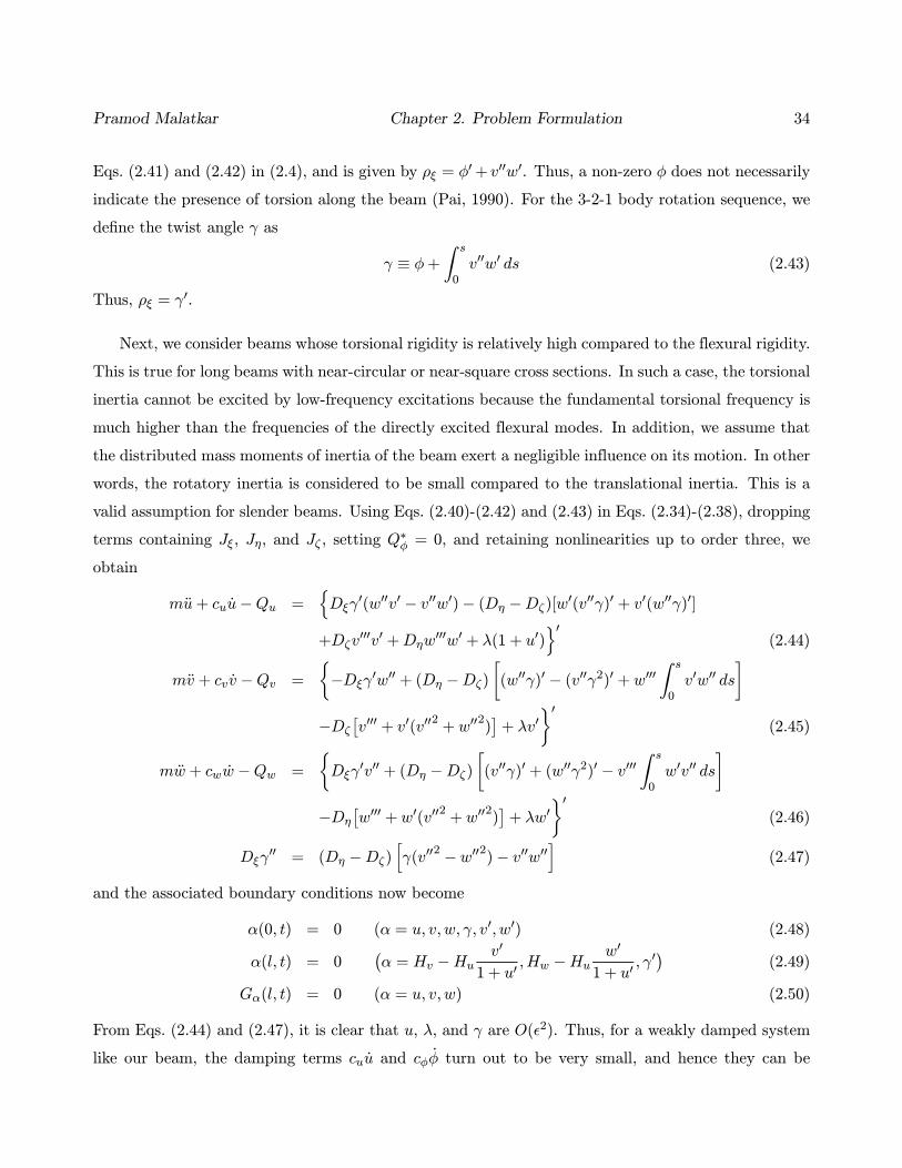
Pramod Malatkar Chapter 2. Problem Formulation 34
Eqs. (2.41) and (2.42) in (2.4), and is given by ρξ = φ + v w . Thus, a non-zero φ does not necessarily
indicate the presence of torsion along the beam (Pai, 1990). For the 3-2-1 body rotation sequence, we
define the twist angle γ as
γ ≡ φ+s
0v w ds (2.43)
Thus, ρξ = γ .
Next, we consider beams whose torsional rigidity is relatively high compared to the flexural rigidity.
This is true for long beams with near-circular or near-square cross sections. In such a case, the torsional
inertia cannot be excited by low-frequency excitations because the fundamental torsional frequency is
much higher than the frequencies of the directly excited flexural modes. In addition, we assume that
the distributed mass moments of inertia of the beam exert a negligible influence on its motion. In other
words, the rotatory inertia is considered to be small compared to the translational inertia. This is a
valid assumption for slender beams. Using Eqs. (2.40)-(2.42) and (2.43) in Eqs. (2.34)-(2.38), dropping
terms containing Jξ, Jη, and Jζ , setting Q∗φ = 0, and retaining nonlinearities up to order three, we
obtain
mu+ cuu−Qu = Dξγ (w v − v w )− (Dη −Dζ)[w (v γ) + v (w γ) ]
+Dζv v +Dηw w + λ(1 + u ) (2.44)
mv + cvv −Qv = −Dξγ w + (Dη −Dζ) (w γ) − (v γ2) + ws
0v w ds
−Dζ v + v (v2+ w
2) + λv (2.45)
mw + cww −Qw = Dξγ v + (Dη −Dζ) (v γ) + (w γ2) − vs
0w v ds
−Dη w +w (v2+ w
2) + λw (2.46)
Dξγ = (Dη −Dζ) γ(v2 − w 2
)− v w (2.47)
and the associated boundary conditions now become
α(0, t) = 0 (α = u, v,w, γ, v , w ) (2.48)
α(l, t) = 0 α = Hv −Hu v
1 + u,Hw −Hu w
1 + u, γ (2.49)
Gα(l, t) = 0 (α = u, v,w) (2.50)
From Eqs. (2.44) and (2.47), it is clear that u, λ, and γ are O( 2). Thus, for a weakly damped system
like our beam, the damping terms cuu and cφφ turn out to be very small, and hence they can be

Pramod Malatkar Chapter 2. Problem Formulation 35
dropped from the equations of motion. Also, we see that if Dη = Dζ , then there will be no coupling
between the flexural and torsional motions. In fact, in such a case, γ = 0.
Using the boundary conditions u(0, t) = 0, Gu(L, t) = 0, γ(0, t) = 0, and γ (L, t) = 0 in Eqs. (2.40),
(2.44), and (2.47), we obtain
u = −12
s
0(v
2+ w
2) ds (2.51)
λ = −Dζv v −Dηw w − 12m
s
l
s
0(v
2+ w
2) ds
..ds−
s
lQu ds (2.52)
γ = −Dη −Dζ
Dξ
s
0
s
lv w ds ds (2.53)
Equation (2.53) shows that the bending-induced twisting is a nonlinear phenomenon. The Lagrange
multiplier λ(s, t) is interpreted as an axial force, necessary to maintain the inextensionality constraint.
Substituting Eqs. (2.51)-(2.53) into Eqs. (2.45), (2.46), and (2.48)-(2.50) and keeping terms up to
order three, we obtain
mv + cvv +Dζviv = Qv + (Dη −Dζ) w
s
lv w ds− w
s
0v w ds
−(Dη −Dζ)2
Dξw
s
0
s
lv w ds ds −Dζ v (v v + w w )
−12m v
s
l
s
0(v
2+ w
2) ds
..ds − v
s
lQu ds (2.54)
mw + cww +Dηwiv = Qw − (Dη −Dζ) v
s
lv w ds− v
s
0w v ds
+(Dη −Dζ)
2
Dξv
s
0
s
lv w ds ds −Dη w (v v + w w )
−12m w
s
l
s
0(v
2+ w
2) ds
..ds − w
s
lQu ds (2.55)
with the boundary conditions now being
v(0, t) = 0, w(0, t) = 0, v (0, t) = 0, w (0, t) = 0 (2.56)
v (l, t) = 0, w (l, t) = 0, v (l, t) = 0, w (l, t) = 0 (2.57)
In the above equations of motion, only cubic nonlinearities are present. The nonlinear term on the right-
hand side of Eqs. (2.54) and (2.55), with the time derivatives, is the inertia nonlinearity arising from

Pramod Malatkar Chapter 2. Problem Formulation 36
the kinetic energy of axial motion. The rest of the nonlinear terms are of the geometric nonlinearity
type and originate from the potential energy stored in bending.
When the beam is subjected only to a transverse base excitation in the y-direction, with all other
external forces except gravity being absent, we have Qv = Qw = 0, Qu = −mg, and v = v+ v0 cos(Ωt),where g (= 9.8 m/s2) denotes the acceleration due to gravity, v is the displacement in the y-direction,
with respect to the base, and v0 and Ω are the amplitude and frequency of the base motion. Also, δv
should be replaced by δv wherever it appears in the above equations, and in Eq. (2.27), cvv should be
replaced by cv ˙v. In Eq. (2.54), mv = m¨v −mv0Ω2 cos(Ωt) = m¨v −mab cos(Ωt), where ab denotes theamplitude of the base acceleration. The equations of motion and boundary conditions now become
mv + cvv +Dζviv = mg[v (s− l) + v ] + (Dη −Dζ) w
s
lv w ds− w
s
0v w ds
−(Dη −Dζ)2
Dξw
s
0
s
lv w ds ds −Dζ v (v v + w w )
−12m v
s
l
s
0(v
2+ w
2) ds
..ds +mab cos(Ωt) (2.58)
mw + cww +Dηwiv = mg[w (s− l) + w ]− (Dη −Dζ) v
s
lv w ds− v
s
0w v ds
+(Dη −Dζ)
2
Dξv
s
0
s
lv w ds ds −Dη w (v v + w w )
−12m w
s
l
s
0(v
2+ w
2) ds
..ds (2.59)
v(0, t) = 0, w(0, t) = 0, v (0, t) = 0, w (0, t) = 0 (2.60)
v (l, t) = 0, w (l, t) = 0, v (l, t) = 0, w (l, t) = 0 (2.61)
where the bar over v has been dropped for ease of notation.

Chapter 3
Parametric System Identification
In this chapter, we propose a simple parametric identification technique for single-degree-of-freedom
(SDOF) nonlinear systems with weak cubic nonlinearities. The proposed technique is related to the
backbone curve method in the sense that it also uses the peak of the frequency-response curve of the
nonlinear system to estimate the model parameters. But the proposed technique is much more simple
and straightforward compared to the backbone curve method. The proposed identification procedure
is outlined in the context of a single-mode response of an externally excited cantilever beam possessing
cubic geometric and inertia nonlinearities and linear and quadratic damping.
3.1 Theoretical Modeling
3.1.1 Equation of Motion
Equations (2.58) and (2.59) governing the nonplanar dynamics of an isotropic, inextensional beam are
simplified to the case of planar motion of a uniform metallic cantilever beam under external excitation.
Following the approach of Anderson, Nayfeh, and Balachandran (1996b) and Tabaddor (2000), we
also include quadratic damping (air drag) in the model, in addition to linear damping, to study its
influence on the beam response. For the natural frequencies, we use the experimental values instead of
the theoretical ones, and thus drop the gravity term from the equation of motion. The model equation
37

Pramod Malatkar Chapter 3. Parametric System Identification 38
used in this study is as follows:
mv + cvv + c v|v|+EIviv = mab cos(Ωt)−EI v (v v ) − 12m v
s
l
∂2
∂t2
s
0v2ds ds (3.1)
and the boundary conditions are
v(0, t) = 0, v (0, t) = 0 (3.2)
v (l, t) = 0, v (l, t) = 0 (3.3)
where m is the beam mass per unit length, l is the beam length, E is Young’s modulus, I is the
area moment of inertia, s is the arclength, t is time, v(s, t) is the transverse displacement, ab is the
acceleration of the supported end of the beam, cv is the coefficient of linear viscous damping per unit
length, c is the coefficient of quadratic damping per unit length, and Ω is the excitation frequency.
And, the prime indicates differentiation with respect to the arclength s, whereas the overdot indicates
differentiation with respect to time t.
3.1.2 Single-Mode Response
The steel beam used in the experiments constitutes a lightly damped, weakly nonlinear system, and
none of its modes is involved in an internal resonance with other modes. We, therefore, assume that
the response of the beam consists essentially of the undamped linear mode whose natural frequency is
closest to the excitation frequency. We refer to this mode as the nth mode whose frequency ωn is then
very close to the excitation frequency Ω. Other modes, not being directly or indirectly excited, will
decay to zero with time due to the presence of damping (Nayfeh and Mook, 1979).
Equations (3.1)-(3.3) are not readily amenable to a closed-form solution. We, therefore, resort to
perturbation methods to obtain an approximate analytical solution. The method of multiple scales
(Nayfeh, 1973b,1981) is used to derive a first-order uniform expansion for the beam response under
primary resonance. Using a method of multiple scales’ model for system identification would lead to
biased parameter estimates at high levels of excitation (Doughty, Davies, and Bajaj, 2002). In the
experiments, the excitation levels are kept low and so we need not be unduly concerned about any bias
creeping into the estimates.
We scale the damping coefficients cv and c and the forcing coefficient ab appearing in Eq. (3.1) in

Pramod Malatkar Chapter 3. Parametric System Identification 39
terms of a small dimensionless parameter ( 1) as follows:
cv2m
= ζ ωn = 2µ (3.4)
c
m= c = c (3.5)
ab = 3f (3.6)
where ζ is the dimensionless linear viscous damping factor corresponding to the nth mode. Also, we
let
v(s, t; ) = v1(s, T0, T2) +3v3(s, T0, T2) + · · · (3.7)
where the Tn (=nt) represent different time scales — T0 being the fast-time scale and T2 the slow-time
scale. The derivatives with respect to t now take the form
d
dt= D0 + D1 +
2D2 + · · · (3.8)
d2
dt2= D20 + 2 D0D1 +
2(D21 + 2D0D2) + · · · (3.9)
where Dn = ∂/∂Tn. Substituting Eqs. (3.4)-(3.9) into Eqs. (3.1)-(3.3) and equating coefficients of like
powers of , we obtain
Order :
D20v1 +EI
mviv1 = 0 (3.10)
v1 = 0 and v1 = 0 at s = 0 (3.11)
v1 = 0 and v1 = 0 at s = l (3.12)
Order 3:
D20v3 +EI
mviv3 = −2D0D2v1 − 2µD0v1 − cD0v1 | D0v1 | −
EI
mv1 v1v1
−12v1
s
lD20
s
0v 21 ds ds + f cos(ΩT0) (3.13)
v3 = 0 and v3 = 0 at s = 0 (3.14)
v3 = 0 and v3 = 0 at s = l (3.15)

Pramod Malatkar Chapter 3. Parametric System Identification 40
Since we are seeking a single-mode response solution, the solution of the first-order problem associated
with Eqs. (3.10)-(3.12) is taken as
v1(s, T0, T2) = A(T2)eiωnT0 + A(T2)e
−iωnT0 Φn(s) (3.16)
where A(T2) is the complex conjugate of A(T2); ωn = r2n EI/ml4, rn is the nth root of the charac-
teristic equation 1+ cos(r) cosh(r) = 0; and Φn(s) denotes the normalized shape of the nth undamped
linear vibration mode, which is given by the following expression:
Φn(s) =1√lcosh
rns
l− cos rns
l+cos rn + cosh rnsin rn + sinh rn
sinrns
l− sinh rns
l
For large n, the numerical evaluation of the rn and Φn(s) requires retention of an increasingly large
number of significant digits because of the presence of hyperbolic (exponential) functions. To avoid this
problem, Dowell (1984) and Dugundji (1988) derived simple expressions for higher vibration modes of
uniform Euler-Bernoulli beams. McDaniel et al. (2002) proposed a method for estimating the natural
frequencies and mode shapes of a multiple-degree-of-freedom system from its forced response vectors.
Substituting Eq. (3.16) into Eq. (3.13) yields
D20v3 +EI
mviv3 = −2iωnΦnD2AeiωnT0 − 2iµωnΦnAeiωnT0 +
1
2f eiΩT0
− EIm
Φn ΦnΦn A3e3iωnT0 + 3A2AeiωnT0
+ 2ω2n Φn
s
l
s
0Φ 2n dsds A3e3iωnT0 +A2AeiωnT0 + cc
− cω2nΦn iAeiωnT0 − iAe−iωnT0 | Φn iAeiωnT0 − iAe−iωnT0 | (3.17)
Here we restrict our discussion to the case of primary resonance of the nth mode (i.e., Ω ≈ ωn). To
express the nearness of this resonance, we introduce the detuning parameter σ defined by Ω = ωn+2σ.
Since the homogeneous problem associated with Eqs. (3.17), (3.14), and (3.15) has a nontrivial solution,
the nonhomogeneous problem has a solution only if the right-hand side of Eq. (3.17) is orthogonal to
every solution of the adjoint homogeneous problem (Nayfeh, 1981). Therefore, demanding that the
right-hand side of Eq. (3.17) be orthogonal to Φn(s) exp(−iωnT0), we obtain
−2iωn (D2A+ µA+ αdcA | A |)− 2αA2A+ 12feiσT2 = 0 (3.18)

Pramod Malatkar Chapter 3. Parametric System Identification 41
where
f = fl
0Φn(s)ds
αd =8ωn3π
l
0Φn(s)
2|Φn(s)| ds
αg =3EI
m
l
0Φn(s)
2Φn(s)2ds
αi = −ω2nl
0
s
0Φn(s)
2ds2
ds
α = αg + αi (3.19)
We note that α is the sum of the geometric (hardening) nonlinearity αg and inertia (softening) non-
linearity αi and thus denotes the effective nonlinearity corresponding to the nth mode. Also, α is not
dimensionless, but rather has dimensions 1/ms2.
Substituting the polar form
A =1
2aei(σT2−γ) (3.20)
into Eq. (3.18), multiplying the result by exp [i (γ − σT2)], and separating real and imaginary parts,we obtain the following autonomous modulation equations:
a = −µa− 12αdc a
2 +f
2ωnsin γ (3.21)
aγ = σa− α
4ωna3 +
f
2ωncos γ (3.22)
where the prime indicates differentiation with respect to T2. Substituting Eq. (3.20) into Eq. (3.16)
and then substituting Eq. (3.16) into Eq. (3.7), we find that the beam response is given by
v(s, t; ) = a(t) cos(Ωt− γ)Φn(s) + · · · (3.23)
3.1.3 Frequency-Response and Force-Response Equations
Periodic solutions of the beam correspond to the fixed points of Eqs. (3.21) and (3.22). To determine
these fixed points, we set the right-hand sides of Eqs. (3.21) and (3.22) equal to zero. Now, these two
equations can be used to obtain the frequency- and force-response diagrams. The frequency-response
diagram is obtained by keeping the forcing amplitude constant while varying the excitation frequency.

Pramod Malatkar Chapter 3. Parametric System Identification 42
In contrast, the force-response diagram is obtained by varying the forcing amplitude while keeping the
excitation frequency constant. In both cases, the displacement amplitude of v(s, t) is plotted versus
the control parameter (either Ω or ab).
We use the following two equations, which were derived by setting the right-hand sides of Eqs. (3.21)
and (3.22) equal to zero, to obtain the frequency-response and force-response diagrams, respectively:
σ1,2 =α
4ωna2 ∓ f2
4ω2na2− µ+
1
2αdc a
2(3.24)
f = 2ωna µ+1
2αdc a
2+ σ − α
4ωna2
2(3.25)
where the subscript 1 and the minus sign refer to the left branch of the frequency-response curve, while
the subscript 2 and the plus sign refer to the right branch.
3.2 Experimental Procedure
We excited a steel beam with the dimensions 19.085”× 12”× 1
32” by a base excitation. The density and
Young’s modulus of the beam were taken as 7810 kg/m3 and 207 GPa, respectively. The beam was
mounted vertically on a steel clamping fixture attached to a MB Dynamics 445 N (100-lb) electrody-
namic shaker. The output of the shaker was measured using a PCB 308B02 accelerometer placed on
the clamping fixture, and the response of the cantilever beam was measured with a 350 Ohm strain
gage mounted approximately 33 mm from the fixed end of the beam. The strain gage formed one
arm of a quarter bridge circuit, and its signal was conditioned using a Measurements Group 2310 sig-
nal conditioning amplifier. The accelerometer signal was conditioned with a PCB 482A10 amplifier.
The accelerometer amplifier and strain gage conditioner were attached in parallel to a Hewlett-Packard
35670A dynamic signal analyzer, which was also used to drive the MB Dynamics SS250 shaker amplifier.
The experiment included four testing sequences related to the third mode and three sequences
related to the fourth mode. Each of these testing sequences was run on a separate day. In five of these
testing sequences, the frequency was swept while the excitation amplitude was held constant, though
the excitation amplitude itself was different for each sequence. In the other two testing sequences, the
excitation amplitude was varied while the excitation frequency was held constant. We waited for a
long time to ensure steady state before taking any measurement.

Pramod Malatkar Chapter 3. Parametric System Identification 43
3.2.1 Linear Natural Frequencies
The natural frequencies of the beam were determined using the frequency-response function of the
signal analyzer. The beam was excited by a 50% burst-chirp low-amplitude excitation, and a uniform
window was used to analyze the power spectra of the accelerometer and strain-gage signals. Peaks
in the amplitude portion of the frequency-response function give the linear natural frequencies of the
beam. To increase confidence in the experimentally obtained linear natural frequencies, we measured
the frequency-response functions at several low excitation levels. No noticeable shifts in the peaks were
observed. In addition, we made sure that the coherence was close to unity at the corresponding peaks.
Also, a periodic checking of the natural frequencies of the beam was done to detect any fatigue damage.
Table 3.1: Experimentally determined third-mode natural frequency.
ab (m/s2) ω3 (Hz)
0.10g 49.078
0.15g 49.094
0.20g 49.094
Before the beginning of each testing sequence, we measured the natural frequency of the corre-
sponding mode (either third or fourth). In Table 3.1, the measured values of the third-mode natural
frequency are listed alongside the value of the base acceleration of the corresponding testing sequence.
In the ab column, g refers to the acceleration due to gravity and has a value equal to 9.8 m/s2. We
note that the value of the estimated third-mode natural frequency is not constant. The minor vari-
ation could be explained by the fact that these measurements were done on separate days, and the
difference is equal to the frequency resolution of the signal analyzer used to make the measurements.
The experimentally measured value of the fourth-mode natural frequency is 96.117 Hz.
3.2.2 Determination of the Beam Displacement
The strain gage essentially measures the strain at the location where it is mounted on the beam. To
measure the beam displacement at that point, we need to convert the strain into displacement. In this
section, we describe the procedure to convert the strain-gage reading into displacement.

Pramod Malatkar Chapter 3. Parametric System Identification 44
From beam theory, we know that the strain experienced by the strain gage is given by
e = yρ (3.26)
where e denotes the strain, ρ denotes the curvature at the location of the strain gage, and y denotes the
distance of the strain gage from the beam’s neutral axis; that is, y = 12b where b is the beam thickness.
Let w(s) denote the steady-state transverse-displacement amplitude of a point a distance s from the
fixed end of the beam. Then, from Eq. (3.23), we can write
w(s) = aΦn(s) (3.27)
The curvature at a distance s from the fixed end is given by
ρ =∂2w
∂s21 +
∂w
∂s
2 − 32(3.28)
For the displacement amplitudes observed in the testing sequences, it was found that the nonlinear
expression for the curvature was not necessary. The linear part by itself determines the displacement
amplitude to a sufficient degree of accuracy. Hence, we use the following linear expression for the
curvature:
ρ ≈ ∂2w
∂s2(3.29)
which is the commonly used expression for curvature in any strength of materials textbook (Timoshenko
and Young, 1968).
Let lsg denote the distance of the strain gage center from the fixed end. Using Eq. (3.27) in
Eq. (3.29), we obtain
ρ |s=lsg = aΦn(lsg) (3.30)
Alternatively, we can determine the strain from the strain-gage reading as follows:
e =4Vout
VexciteGKg(3.31)
where Vout denotes the strain-gage amplifier output in volts, Vexcite denotes the bridge excitation voltage
in volts, G denotes the gain of the strain-gage signal conditioner, and Kg denotes the gage factor of
the strain gage. Subsitituting Eqs. (3.30) and (3.31) into Eq. (3.26), we obtain
a =8
VexciteGKgbΦn(lsg)Vout

Pramod Malatkar Chapter 3. Parametric System Identification 45
which when substituted into Eq. (3.27) gives
w(s) =8Φn(s)
VexciteGKgbΦn(lsg)Vout (3.32)
Therefore, we only need to multiply the strain-gage reading Vout by a constant to obtain the displace-
ment amplitude w at a given s.
Table 3.2: Some constants and their values.
Constant Vexcite G Kg b lsg
Value 10 V 1000 2.095 0.794 mm 32.56 mm
The values of the constants appearing in Eq. (3.32) are listed in Table 3.2. We use wl to denote the
displacement amplitude of the beam tip where s = l.
3.3 Parameter Estimation Procedure
We estimate the parameters (ζ, c, α) describing the weakly damped, weakly nonlinear beam system
from the experimental frequency-response results. We know that, for a given excitation level, the
amplitude at the peak of the corresponding frequency-response curve depends on the damping value
(Nayfeh and Mook, 1979). And the effect of the nonlinearity is essentially to shift the peak away from
the natural frequency ωn. For a system with hardening nonlinearity, the peak is shifted to the right;
and in the case of a softening nonlinearity it is shifted to the left. The magnitude of the shift depends
on the strength of the nonlinearity. Thus, knowing the amplitude at the peak and the frequency shift,
it is possible to estimate the damping coefficient(s) and the effective nonlinearity of a system. The
detailed estimation procedure is described in the following subsections.
Table 3.3 lists the coordinates of the peaks of the experimentally obtained third-mode frequency-
response curves for different base acceleration levels. The peak displacement amplitude of the beam tip
is denoted by w∗l , and Ω∗ is used to denote the value of the excitation frequency at the peak. We note
that ω3, given in Table 3.1, denotes the linear resonance frequency, whereas Ω∗ (in Table 3.3) denotes
the nonlinear resonance frequency.

Pramod Malatkar Chapter 3. Parametric System Identification 46
Table 3.3: Coordinates of the peak of the frequency-response curve.
ab (m/s2) Ω∗ (Hz) w∗l (mm)
0.10g 48.963 2.415
0.15g 48.917 3.220
0.20g 48.885 3.876
3.3.1 Estimation of the Damping Coefficients
Linear Damping Model
We can easily estimate the linear viscous damping coefficient µ from the experimental frequency-
response curve. For the linear damping model (c = 0), it follows from Eq. (3.24) that the peak of the
frequency-response curve corresponds to
µ =f
2ωna∗(3.33)
where a∗ denotes the value of a at the peak. So, by measuring a∗ and knowing the values of f and
ωn, we can estimate the linear damping coefficient. Using the definitions of µ, f , and w(s), we rewrite
Eq. (3.33) in terms of physical quantities as
ζ =abξnΦn(l)
2ω2nw∗l
× 103 (3.34)
where ξn =l0 Φn(s)ds, ωn is the nth natural frequency in rad/sec, and w
∗l denotes the peak displace-
ment amplitude of the beam tip in mm.
Nonlinear Damping Model
With the addition of quadratic damping (air drag), we complicate our model. But the advantage, as
we would see later, is that the experimental and theoretical frequency- and force-response curves are
in much better agreement when compared to the linearly damped case.
At the peak of the frequency-response curve, it follows from Eq. (3.24) that
µ+1
2αdc a
∗ =f
2ωna∗(3.35)

Pramod Malatkar Chapter 3. Parametric System Identification 47
where a∗ denotes the value of a at the peak. But now we have two unknowns (µ and c) and just one
equation. We, therefore, use results of two testing sequences to determine the damping coefficients c
and µ. Using Eq. (3.35) for two testing sequences, denoted by subscripts 1 and 2, we have
c =1
αd(a∗2 − a∗1)
f2ωna∗2
− f1ωna∗1
µ =f2
2ωna∗2− 12αdc a
∗2
In terms of physical quantities, we have
c =ξnΦn(l)
2
αd(w∗l2 − w∗l1)
ab2ωnw∗l2
− ab1ωnw∗l1
× 106 (3.36)
ζ =ab2ξnΦn(l)
2ω2nw∗l2
× 103 − αdw∗l2 c
2ωnΦn(l)× 10−3 (3.37)
where w∗l1 and w∗l2 denote the peak displacement amplitudes of the beam tip (in mm) corresponding
to the testing sequences 1 and 2, respectively.
3.3.2 Nonlinearity Estimation
At the peak of the frequency-response curve, it follows from Eqs. (3.24), (3.33), and (3.35) that
α =4ωnσ
∗
a∗2
where a∗ and σ∗ denote the values of a and σ, respectively, at the peak. In terms of physical quantities,
we have
α =4ωnΦn(l)
2(Ω∗ − ωn)w∗2l
× 106 (3.38)
where w∗l and Ω∗ denote the tip displacement amplitude (in mm) and excitation frequency (in rad/sec)
at the peak, respectively. We note that Eq. (3.38) is applicable to both the linear as well as the nonlinear
damping models.
3.3.3 Curve-Fitting the Frequency-Response Data
The parameter values can also be estimated by curve-fitting the experimental frequency-response data
points. This is the approach used by Krauss and Nayfeh (1999a,b) to estimate nonlinear parameters

Pramod Malatkar Chapter 3. Parametric System Identification 48
of a system. We used the MATLAB function nlinfit, which performs a nonlinear least-squares data
fitting using a Gauss-Newton method, to fit a theoretical model to the experimental data points. More
specifically, we estimated the parameters in Eq. (3.24) by fitting it to the experimental frequency-
response data set. A drawback of the curve-fitting method is its sensitivity to and dependence on the
initial guesses. In the next section, we compare the results obtained, for the fourth mode, using the
proposed estimation technique with those obtained by the curve-fitting method.
3.3.4 Fixing f and ωn
48.6 48.8 49 49.2 49.4 49.6 49.8
0.5
1
1.5
2
2.5
3
3.5
4
Excitation Frequency, Ω (in Hz)
Tip
Dis
plac
emen
t Am
plitu
de, w
l (in
mm
) TheoreticalBackward Sweep (Expt.)Forward Sweep (Expt.)
Figure 3.1: Experimentally and theoretically obtained third-mode frequency-response curves for
ab = 0.2g and ω3 = 49.094 Hz using the linear damping model.
There were some differences between the experimentally and theoretically obtained frequency-response
curves. In Fig. 3.1, we have plotted an experimentally observed frequency-response curve along with
the theoretical one for the third mode. We used the theoretical value of α, the estimated value of µ
(and c), and the experimentally determined values of f and ω3 in Eq. (3.24) to obtain the theoretical
frequency-response curve. The value of f was determined from the accelerometer reading, and ω3
was determined using the frequency-response function of the signal analyzer. We observe in Fig. 3.1
that the theoretically obtained frequency-response curve is to the right of the experimental one. This

Pramod Malatkar Chapter 3. Parametric System Identification 49
48.6 48.8 49 49.2 49.4 49.6 49.8
0.5
1
1.5
2
2.5
3
3.5
4
Excitation Frequency, Ω (in Hz)
Tip
Dis
plac
emen
t Am
plitu
de,
wl (
in m
m) Theoretical
Backward Sweep (Expt.)Forward Sweep (Expt.)
Figure 3.2: Experimentally and theoretically obtained third-mode frequency-response curves for
ab = 0.23g and ω3 = 49.06 Hz using the linear damping model.
indicates that the value of ω3 used in Eq. (3.24) needs to be lowered. Also, we observe that the spike
in the experimental frequency-response curve is wider than the theoretical one. This indicates that the
value of f used in Eq. (3.24) needs to be increased.
For better agreement between the third-mode experimental and theoretical frequency-response
results, we had to lower the value of ω3 by nearly 0.05 Hz, which is around 0.1% of the measured
third natural frequency, and we had to increase the value of f by nearly 15% for the linear damping
model and by 8% for the nonlinear damping model. The probable reason for the shift in the frequency-
response curve could be the non-inclusion of gravity in the equation of motion and/or of higher-order
terms in the modulation equations. But on investigation later, we found that inclusion of higher-order
terms did not affect the results much. Also, with the addition of gravity, which tends to lower the
natural frequencies, the problem still persisted. We believe the assumption of ideal-clamp boundary
condition could be contributing to the shift in the results. Tabaddor (2000) studied the influence of
nonideal-clamp boundary conditions and found significant changes in the model behavior. This needs
to be studied further in the present context. On the other hand, we believe the difference in the
value of f is probably due to improper calibration of the accelerometer and/or due to an error in the
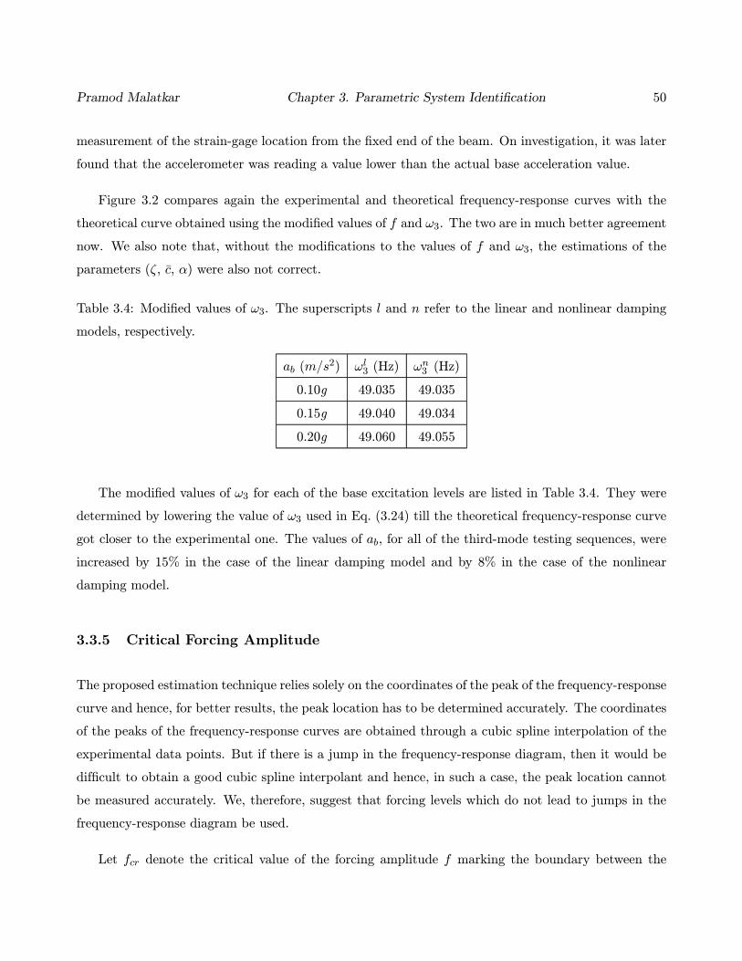
Pramod Malatkar Chapter 3. Parametric System Identification 50
measurement of the strain-gage location from the fixed end of the beam. On investigation, it was later
found that the accelerometer was reading a value lower than the actual base acceleration value.
Figure 3.2 compares again the experimental and theoretical frequency-response curves with the
theoretical curve obtained using the modified values of f and ω3. The two are in much better agreement
now. We also note that, without the modifications to the values of f and ω3, the estimations of the
parameters (ζ, c, α) were also not correct.
Table 3.4: Modified values of ω3. The superscripts l and n refer to the linear and nonlinear damping
models, respectively.
ab (m/s2) ωl3 (Hz) ωn3 (Hz)
0.10g 49.035 49.035
0.15g 49.040 49.034
0.20g 49.060 49.055
The modified values of ω3 for each of the base excitation levels are listed in Table 3.4. They were
determined by lowering the value of ω3 used in Eq. (3.24) till the theoretical frequency-response curve
got closer to the experimental one. The values of ab, for all of the third-mode testing sequences, were
increased by 15% in the case of the linear damping model and by 8% in the case of the nonlinear
damping model.
3.3.5 Critical Forcing Amplitude
The proposed estimation technique relies solely on the coordinates of the peak of the frequency-response
curve and hence, for better results, the peak location has to be determined accurately. The coordinates
of the peaks of the frequency-response curves are obtained through a cubic spline interpolation of the
experimental data points. But if there is a jump in the frequency-response diagram, then it would be
difficult to obtain a good cubic spline interpolant and hence, in such a case, the peak location cannot
be measured accurately. We, therefore, suggest that forcing levels which do not lead to jumps in the
frequency-response diagram be used.
Let fcr denote the critical value of the forcing amplitude f marking the boundary between the

Pramod Malatkar Chapter 3. Parametric System Identification 51
values of f leading to jumps and those not leading to jumps. For the case of linear damping (c = 0),
fcr is given by
fcr = 8µωn2µωn
3√3|α|
which can be rewritten in terms of physical quantities as follows:
abcr =8ζω3n3ξn
2√3ζ
|α|where abcr denotes the critical base acceleration. A detailed derivation procedure of the critical forcing
amplitude is presented in Chapter 4. To determine abcr , we use the theoretical value of α (Eq. (3.19))
and the experimental values of ζ and ωn in the above equation. Here, we reiterate that, to obtain good
results, a base excitation amplitude ab < abcr be used.
3.4 Results
In this section, we first present the estimates of the parameters (ζ, c, α) obtained using the proposed
estimation technique. To validate the proposed estimation technique, we compare the experimentally
and theoretically obtained third-mode frequency- and force-response curves. The theoretical frequency-
and force-response curves are obtained using the estimated parameter values in Eqs. (3.24) and (3.25),
respectively. Theoretical results for both the linear as well as the nonlinear damping models are
presented. To further boost the confidence in the proposed estimation technique, we compare its
fourth-mode frequency- and force-response curves with those obtained using the curve-fitting method.
3.4.1 Third-Mode Estimation Results
For the linear damping model, the value of the linear viscous damping factor ζ is estimated using
Eq. (3.34). The estimated values of the damping factor ζ obtained using the experimental results of
the third-mode frequency-response testing sequences are listed in Table 3.5. We note that the value of ζ
is not constant but shows a variation of approximately 12%. This is expected as damping is essentially
a complex phenomenon, which depends upon the frequency and amplitude of vibration.
For the nonlinear damping model, the values of the damping coefficients ζ and c are estimated
using Eqs. (3.36) and (3.37). The values of the linear viscous damping factor ζ and the quadratic

Pramod Malatkar Chapter 3. Parametric System Identification 52
Table 3.5: Estimated values of the third-mode viscous damping factor ζ of the linear damping model.
ab (m/s2) ζ
0.10g 1.251× 10−30.15g 1.407× 10−30.20g 1.557× 10⁻³
Table 3.6: Estimated values of the third-mode damping coefficients ζ and c of the nonlinear damping
model.
ab (m/s2) ζ c (1/m)
0.10g 7.341× 10⁻⁴ 0.677
0.15g 6.975× 10⁻⁴ 0.732
0.20g 6.262× 10⁻⁴ 0.801
damping coefficient c obtained using the experimental results of the third-mode frequency-response
testing sequences are listed in Table 3.6. We note that the values of ζ and c are not constant but show
a variation of around 7%.
Table 3.7: Estimated values of the third-mode effective nonlinearity α. The superscripts l and n refer
to the linear and nonlinear damping models, respectively.
ab (m/s2) αl (1/ms2) αn (1/ms2)
0.10g −7.888× 10⁸ −7.888× 1080.15g −7.581× 10⁸ −7.210× 1080.20g −7.447× 10⁸ −7.233× 10⁸
For both of the linear as well as the nonlinear damping models, the value of the effective nonlinear-
ity α is estimated using Eq. (3.38). Table 3.7 lists the estimated values of α for each of the third-mode
frequency-response testing sequences. There is a slight variation in the estimated values of α, but all of
them are close to the theoretical value of α = −7.543× 10⁸ obtained using Eq. (3.19). The differencein the values of αl and αn is due to the difference in the values of ωl3 and ω
n3 (refer to Table 3.4).

Pramod Malatkar Chapter 3. Parametric System Identification 53
48.6 48.8 49 49.2 49.4 49.6
0.5
1
1.5
2
2.5
3
3.5
4
Excitation Frequency, Ω (in Hz)
Tip
Dis
plac
emen
t Am
plitu
de,
wl (
in m
m) Theoretical (Linear Damping)
Backward Sweep (Expt.)Forward Sweep (Expt.)
ab= 0.2g
ab= 0.15g
ab= 0.1g
Figure 3.3: Experimentally and theoretically obtained third-mode frequency-response curves for
ab = 0.1g, 0.15g, and 0.2g using the linear damping model.
48.6 48.8 49 49.2 49.4 49.6
0.5
1
1.5
2
2.5
3
3.5
4
Excitation Frequency, Ω (in Hz)
Tip
Dis
plac
emen
t Am
plitu
de,
wl (
in m
m) Theoretical (NL Damping)
Backward Sweep (Expt.)Forward Sweep (Expt.)
ab= 0.2g
ab= 0.15g
ab= 0.1g
Figure 3.4: Experimentally and theoretically obtained third-mode frequency-response curves for
ab = 0.1g, 0.15g, and 0.2g using the nonlinear damping model.

Pramod Malatkar Chapter 3. Parametric System Identification 54
0 100 200 300 400 5000
1
2
3
4
5
Base Acceleration, ab (in milli−g)
Tip
Dis
plac
emen
t Am
plitu
de,
wl (
in m
m)
Theoretical (Linear Damping)Theoretical (Nonlinear Damping)Backward Sweep (Expt.)Forward Sweep (Expt.)
Figure 3.5: Experimentally and theoretically obtained third-mode force-response curves using the linear
and nonlinear damping models for Ω = 48.891 Hz.
Next, we compare the experimentally and theoretically obtained third-mode frequency- and force-
response curves. The theoretical curves are obtained using Eqs. (3.24) and (3.25). For parameters ap-
pearing in these equations, corresponding values estimated from the experimental results are used. Fig-
ure 3.3 compares the experimentally and theoretically obtained third-mode frequency-response curves
using the linear damping model. The parameter values shown in Tables 3.5 and 3.7 were used to
obtain the theoretical curves. Figure 3.4 compares the experimentally and theoretically obtained third-
mode frequency-response curves using the nonlinear damping model. The parameter values shown in
Tables 3.6 and 3.7 were used to obtain the theoretical curves. Figure 3.5 compares the experimen-
tal third-mode force-response curve with those obtained theoretically using the linear and nonlinear
damping models. The agreement between the experimental results and the results obtained using
the theoretical models is very good. Especially, the nonlinear damping model does a very good job
predicting values very close to all of the experimental data points. Also, in the case of the linear
damping model, if a value of ζ estimated for one particular excitation amplitude is used in plotting the
theoretical frequency-response curve of another excitation amplitude, then it leads to an overshoot or
undershoot of the peak of the curve. This is not the case with the nonlinear damping model. Any pair

Pramod Malatkar Chapter 3. Parametric System Identification 55
48.6 48.8 49 49.2 49.4 49.60.5
1
1.5
2
2.5
3
3.5
4
4.5
Excitation Frequency, Ω (in Hz)
Theoretical (NL Damping)Theoretical (Linear Damping)Backward Sweep (Expt.)Forward Sweep (Expt.)(in
mm
) w
lT
ip D
ispl
acem
ent A
mpl
itude
,
Figure 3.6: Overshoot in the peak of the third-mode frequency-response curve obtained using the linear
damping model.
of (ζ, c) values from Table 3.6 can be used to correctly predict the response curves of other testing
sequences. This behavior is shown in Fig. 3.6, where the estimated values of ζ (and c) from the second
testing sequence (ab = 0.15g) were used to plot the theoretical frequency-response curve of the third
testing sequence (ab = 0.2g). We observe an overshoot using the linear damping model, whereas the
results obtained using the nonlinear damping model match very well the corresponding experimental
results.
3.4.2 Comparison with Curve-Fitting Method
To further validate the proposed estimation technique, we compare the fourth-mode frequency- and
force-response curves obtained using the proposed technique with those obtained using the curve-fitting
method.
Tables 3.8 and 3.9 list the estimated values of the parameters of the linear and nonlinear damping
models obtained using the proposed estimation technique and the curve-fitting method. Using these
estimated values, we plotted the frequency- and force-response curves for the linear and nonlinear

Pramod Malatkar Chapter 3. Parametric System Identification 56
Table 3.8: Comparison of the estimates of the damping factor ζ and the effective nonlinearity α for
the fourth mode using the linear damping model. The superscripts p and cf refer to the proposed
estimation technique and the curve-fitting method, respectively.
ab (m/s2) ζp αp (1/ms2) ζcf αcf (1/ms2)
0.075g 6.951× 10⁻⁴ −1.621× 10¹⁰ 6.955× 10⁻⁴ −1.766× 10100.100g 7.220× 10⁻⁴ −1.374× 10¹⁰ 7.220× 10⁻⁴ −1.430× 10¹⁰
Table 3.9: Comparison of the estimates of the fourth-mode damping coefficients ζ and c and the
effective nonlinearity α using the nonlinear damping model. The superscripts p and cf refer to the
proposed estimation technique and the curve-fitting method, respectively.
ab (m/s2) ζp c p (1/m) αp (1/ms2) ζcf c cf (1/m) αcf (1/ms2)
0.075g 5.810e-4 0.624 -1.621e10 6.157e-4 0.471 -1.751e10
0.100g 5.810e-4 0.624 -1.300e10 6.083e-4 0.501 -1.325e10
95.8 95.9 96 96.1 96.2 96.3 96.4
0.2
0.3
0.4
0.5
0.6
0.7
0.8
Excitation Frequency, Ω (in Hz)
Tip
Dis
plac
emen
t Am
plitu
de,
wl (
in m
m) Theoretical (Linear Damping)
Curve Fitting (Linear Damping)Backward Sweep (Expt.)Forward Sweep (Expt.)
ab= 0.1g
ab= 0.075g
Figure 3.7: Comparison of the fourth-mode frequency-response curves obtained using the proposed
technique and the curve-fitting method for ab = 0.075g and 0.1g using the linear damping model.

Pramod Malatkar Chapter 3. Parametric System Identification 57
95.8 95.9 96 96.1 96.2 96.3 96.4
0.2
0.3
0.4
0.5
0.6
0.7
0.8
Excitation Frequency, Ω (in Hz)
Tip
Dis
plac
emen
t Am
plitu
de,
wl (
in m
m) Theoretical (NL Damping)
Curve Fitting (NL Damping)Backward Sweep (Expt.)Forward Sweep (Expt.)
ab= 0.1g
ab= 0.075g
Figure 3.8: Comparison of the fourth-mode frequency-response curves obtained using the proposed
technique and the curve-fitting method for ab = 0.075g and 0.1g using the nonlinear damping model.
Note: In the legend, NL stands for Nonlinear.
0 200 400 600 800 10000
0.5
1
1.5
2
Base Acceleration, ab (in milli−g)
Tip
Dis
plac
emen
t Am
plitu
de,
wl (
in m
m)
Theoretical (Linear Damping)Curve Fitting (Linear Damping)Theoretical (Nonlinear Damping)Curve Fitting (Nonlinear Damping)Backward Sweep (Expt.)Forward Sweep (Expt.)
Figure 3.9: Comparison of the fourth-mode force-response curves obtained using the proposed technique
and the curve-fitting method for Ω = 95.844 Hz using the linear and nonlinear damping models.
damping models, which are displayed in Figs. 3.7-3.9. The agreement between the results obtained
with the two different techniques is very good.

Pramod Malatkar Chapter 3. Parametric System Identification 58
The linear damping model was found to have a serious drawback. The value of the linear viscous
damping factor ζ was also determined experimentally using the half-power method and was found to
be ζ = 6.569×10⁻⁴. But the values of ζ estimated using the linear damping model are higher than themeasured experimental value. On the other hand, the values of ζ estimated by the nonlinear damping
model are less than the measured experimental value, as expected.
3.5 Closure
A simple and straightforward parametric identification procedure for estimating the nonlinear para-
meters describing a single-mode response of a weakly nonlinear cantilever beam is presented. Using
information of the peak locations of one or two (depending on the damping model) frequency-response
curves, one can estimate to a sufficient degree of accuracy the parameters of the nonlinear model de-
scribing the cantilever beam system. This method is applicable to any SDOF weakly nonlinear system
with cubic geometric and inertia nonlinearities. However, we note that the proposed method cannot
be used to estimate the individual geometric and inertia nonlinearity contributions.
The results obtained using the linear and nonlinear damping models are qualitatively similar but
quantitatively different. For the linear viscous damping factor, the linear damping model estimated
a value much higher than the one determined experimentally using the half-power method. Also, the
theoretical frequency-response curve obtained using the linear damping model does not pass through
all of the experimental data points. This shows that a linear damping model does not model the beam
system well. It is reasonable to assume that large deflections of a blunt body like the beam would give
rise to significant air damping, which is proportional to the square of the velocity. So, inclusion of the
quadratic damping term seems physically justified. This justification was strengthened by the fact that
the nonlinear damping model with a quadratic damping term was able to predict results close to the
experimental data points; it also estimated for the linear viscous damping factor a value less than the
measured experimental value, as expected.
The estimated value of the effective nonlinearity using the proposed estimation technique is close
to the theoretical value; it also leads to a good agreement between the experimentally and theoretically
obtained force-response curves. Results obtained using the proposed technique are similar to those
obtained by the curve-fitting method.

Pramod Malatkar Chapter 3. Parametric System Identification 59
The classic backbone curve method requires determination of peak locations of multiple frequency-
response curves corresponding to different forcing levels and hence is time consuming. On the other
hand, the proposed method is simple and also demonstrates that the effective nonlinearity can be
determined accurately from the peak location of a single frequency-response curve. In addition, the
proposed method is more direct and straightforward and does not involve any least-squares curve
fitting. Finally, the new estimation technique is also very robust, which is demonstrated by the fact
that it led to a very good agreement between the experimentally and theoretically obtained frequency-
and force-response curves for both the third mode as well as the fourth mode.

Chapter 4
Determination of Jump Frequencies
It is a well-known fact that the nonlinearity present in a system leads to jumps in the frequency- and
force-response curves (Nayfeh and Mook, 1979). As shown in Fig. 4.1, the frequency-response curve
of a Duffing oscillator is bent either to the left or to the right, depending on whether the type of the
nonlinearity is softening or hardening. The bending of the frequency-response curve leads to a jump
in the response amplitude when the excitation frequency is swept from left-to-right or right-to-left.
The response amplitude increases at a jump-up point and decreases at a jump-down point. Between
the jump points, multiple solutions exist for a given value of the excitation frequency, and the initial
conditions determine which of these solutions represents the actual response of the system. The jump
points of a frequency-response curve coincide with the turning points of the curve where saddle-node
bifurcations occur. The goal of this chapter is to determine the minimum forcing amplitude that would
lead to jumps in the frequency-response curves of single-degree-of-freedom (SDOF) nonlinear systems
and to also locate the jump-up and jump-down points in the frequency-response curve when the forcing
amplitude is above the minimum value.
Friswell and Penny (1994) and Worden (1996) computed the bifurcation points of the frequency-
response curve of a Duffing oscillator with linear damping. They used the method of harmonic balance
to obtain the frequency-response function. To compute the jump frequencies, Worden (1996) set
the discriminant of the frequency-response function, which is a cubic polynomial in the square of
the amplitude, equal to zero, while Friswell and Penny (1994) used a numerical approach based on
Newton’s method. Their first-order approximation results agree well with the “exact” results. But
60

Pramod Malatkar Chapter 4. Jump Frequencies 61
−40 −20 0 20 400
1
2
3
4
5
6
7
8
9x 10
−3
σ
a
(a)
SN
SN
−40 −20 0 20 400
1
2
3
4
5
6
7
8
9x 10
−3
σ
a
(b) SN
SN
Figure 4.1: Typical frequency-response curves of a Duffing oscillator with (a) softening nonlinearity and
(b) hardening nonlinearity. Dashed lines (- -) indicate unstable solutions and SN refers to a saddle-node
bifurcation.
for systems with higher-order geometric, inertia, and/or damping nonlinearities, a more general and
simple method of determining the jump frequencies is required. In this chapter, we present two methods
based on the elimination theory of polynomials (Griffiths, 1947; Wee and Goldman, 1995a), which can
be used to determine both the critical forcing amplitude as well as the jump frequencies in the case
of SDOF nonlinear systems. Also, the methods are devoid of convergence problems associated with
bad initial guesses and have the potential of being applicable to multiple-degree-of-freedom (MDOF)
nonlinear systems (Wee and Goldman, 1995b; Cox, Little, and O’Shea, 1997). The proposed methods
are outlined in the context of a single-mode response of an externally excited cantilever beam possessing
cubic geometric and inertia nonlinearities and linear and quadratic damping.
4.1 Theory
4.1.1 Frequency-Response Function
As the cantilever beam constitutes a weakly damped, weakly nonlinear system, we use the method of
multiple scales (Nayfeh, 1981) to derive the modulation equations governing the amplitude and phase
of the excited mode of the cantilever beam. In the process of deriving the modulation equations, we

Pramod Malatkar Chapter 4. Jump Frequencies 62
define the following quantities:
µ ≡ ζωn , σ ≡ Ω− ωn , f ≡ abl
0Φn ds , c ≡ 4ωn
3πc
l
0Φ2n|Φn| ds
where ζ is the linear viscous damping factor, ωn is the nth natural frequency of the beam, Ω is the
excitation frequency, ab is the base acceleration, l is the length of the beam, s is the arclength, Φn(s) is
the normalized nth mode shape, and c is the quadratic damping coefficient per unit mass and length.
Seeking a first-order uniform expansion of the transverse displacement v(s, t) of the beam, we obtain
v(s, t) ≈ a(t) cos(Ωt− γ)Φn(s) + · · ·
and the modulation equations governing the amplitude a and phase γ of the response are given by
a = −µa− c a2 + f
2ωnsin γ (4.1)
aγ = σa− α
4ωna3 +
f
2ωncos γ (4.2)
where α is the effective nonlinearity comprising the contributions of the geometric and inertia nonlin-
earities, and the overdot indicates differentiation with respect to time t. A detailed description of the
derivation of the modulation equations is given in Chapter 3.
Periodic solutions of the beam correspond to the fixed points of Eqs. (4.1) and (4.2). To determine
these fixed points, we set the right-hand sides of Eqs. (4.1) and (4.2) equal to zero. We, thus, obtain the
following frequency-response function relating the response amplitude a and the excitation frequency
Ω (or σ):
σ1,2 =α
4ωna2 ∓ f2
4ω2na2− (µ+ c a)2 (4.3)
where the subscript 1 and the ‘—’ sign refer to the left branch of the frequency-response curve, while the
subscript 2 and the ‘+’ sign refer to the right branch. Equation (4.3) can be rewritten in polynomial
form as
F(a,σ) = a6 + pa4 + qa3 + ra2 + s = 0 (4.4)
where
p =16ω2nα2
(c2 − α
2ωnσ) , q =
32ω2nα2
µc , r =16ω2nα2
(µ2 + σ2) , s = −4f2
α2

Pramod Malatkar Chapter 4. Jump Frequencies 63
The frequency-response function can also be written as a polynomial function in σ as follows:
F(a,σ) = pσ2 + qσ + r = 0 (4.5)
where
p =16ω2nα2
a2 , q = −8ωnαa4 , r = a6 − 4f
2
α2+16ω2nα2
(c2a4 + 2cµa3 + µ2a2)
4.1.2 Sylvester Resultant
The resultant of two polynomials is defined as the product of all of the differences between the roots
of the polynomials and is a polynomial in the coefficients of the two polynomials (Griffiths, 1947).
Consider two polynomials f(x) and g(x) defined as
f(x) ≡n
i=0
aixi, an = 0, g(x) ≡
m
i=0
bixi, bm = 0
Then, the Sylvester resultant of f(x) and g(x), denoted by R(f, g), is given by (Wee and Goldman,1995a)
R(f, g) =
an an−1 . . . . . . a1 a0 0 . . . . . . 0
0 an an−1 . . . . . . a1 a0 0 . . . 0
. . . . . . . . . . . . . . . . . . . . .
0 . . . 0 an an−1 . . . . . . . . . . . . a0
bm bm−1 . . . b1 b0 0 . . . . . . . . . 0
0 bm bm−1 . . . b1 b0 0 . . . . . . 0
. . . . . . . . . . . . . . . . . . . . .
0 . . . . . . 0 bm bm−1 . . . . . . . . . b0
A necessary and sufficient condition for f(x) and g(x) to have a common root is that the resultant
R(f, g) be equal to zero (Griffiths, 1947). The discriminant ∆ of a polynomial f(x), of order m, is
related to the resultant R(f, f ) in the following manner:
R(f, f ) = (−1) 12m(m−1)am∆
where am is the coefficient of the xm term in the polynomial f(x). We know that f(x) = 0 has two
equal roots iff f(x) = 0 and f (x) = 0 have a common root, and hence iff R(f, f ) = 0. We use thisidea to determine the critical forcing amplitude and jump frequencies.

Pramod Malatkar Chapter 4. Jump Frequencies 64
4.1.3 Critical Forcing Amplitude
For a low excitation amplitude, we do not observe the jump phenomenon and the frequency-response
curve is single-valued; that is, for every value of Ω there is a unique value of a. But in the case of a
large excitation amplitude, we observe jumps, and for a range of Ω values there exist multiple values of
a for a given value of Ω, as seen in Fig. 4.1. Let fcr denote the critical value of f marking the boundary
between the values of f leading to jumps and those not leading to jumps. The frequency-response curve
for f = fcr has an inflection point, which we denote by (σcr, acr), where the frequency-response function
F(a,σcr) = 0 has three positive real roots equal to acr. Therefore, the derivative of the frequency-
response function with respect to the response amplitude a, denoted by F (a,σcr) = 0, has two real
roots equal to acr, which requires that the resultant R(F ,F ) be equal to zero at the inflection point
(σcr, acr). Thus, using Eq. (4.5), we obtain
S(acr) ≡ R(F ,F )a=acr
=6
i=0
biaicr = 0 (4.6)
where
b0 = 144 c2µ2ω4n , b1 = 384 c
3µω4n , b2 = 64ω2n(α
2µ2 + 4 c4ω2n) ,
b3 = 168 cα2µω2n , b4 = 96 c
2α2ω2n , b5 = 0 , b6 = −3α4
We now have a sextic polynomial equation in the response amplitude at the inflection point acr. Using
the resultant, we basically eliminate σcr and obtain a polynomial equation in acr only. By using
Eq. (4.4), we can eliminate acr and obtain a polynomial equation in σcr, but that would involve a more
number of computations. Also, in that case spurious solutions appear while solving for σcr.
Knowing the bi, one can easily compute the value of acr numerically. Of the six roots of S(acr) = 0,only one turns out to be real and positive. Once we know the value of acr, substituting it into
F (a,σcr) = 0 gives us the critical excitation frequency σcr. Using the values of σcr and acr in
Eqs. (4.4) or (4.5), we obtain the critical forcing amplitude fcr.
For the case of linear damping (c = 0), a closed-form solution for the critical forcing amplitude is
possible. The corresponding expressions of fcr, acr, and σcr are as follows:
fcr = 8µωn2µωn
3√3|α| , acr =
8µωn√3|α| , σcr = ±
√3µ
where the ‘+’ sign is for systems with effective hardening nonlinearity (i.e., α > 0), and the ‘—’ sign is
for systems with effective softening nonlinearity (i.e., α < 0).

Pramod Malatkar Chapter 4. Jump Frequencies 65
4.1.4 Jump Frequencies
For f > fcr, we observe jumps in the frequency-response curve, as seen in Fig. 4.1. At the jump
points, which we denote by (σ∗, a∗), the frequency-response function F(a,σ∗) = 0 has two positive realroots equal to a∗, which requires that the resultant R(F ,F ) be equal to zero at those points. Using
Eq. (4.5), we thus obtain a twelfth-order polynomial equation in a∗ as follows:
S(a∗) ≡ R(F ,F )a=a∗ =
12
i=0
ciaia=a∗ = 0 (4.7)
where the ci are functions of known physical quantities. The values of a∗ can be easily computed
numerically. Of the twelve roots of S(a∗) = 0, only two turn out to be real and positive. Once we
know the value of a∗, substituting it into F (a,σ∗) = 0 gives us the the jump frequency σ∗. But for
each value of a∗, we obtain two values of σ∗, one of which is spurious. To pin-point the spurious σ∗
solution, we check if F(a,σ∗) = 0 leads to two positive real roots equal to a∗. If it does not, then thatparticular σ∗ solution is spurious and is discarded. Alternatively, we could also determine σ∗ using
Eq. (4.3). The knowledge of the type of nonlinearity can be used to decide whether the jump points
lie on the left or the right branch.
4.1.5 Grobner Basis
A Grobner basis for the polynomials f1, f2, . . . , fn comprises a set of polynomials G1,G2, . . . ,Gmthat have the same collection of roots as the original polynomials (Cox et al., 1997). Like the Sylvester
resultant, the Grobner bases also can be used to determine the critical forcing amplitude and jump
frequencies. The advantage of using Grobner bases over resultants is that we do not obtain any spurious
solutions while solving for the jump frequencies σ∗. But in general, resultants are more efficient than
Grobner bases.
To determine the critical forcing amplitude, we use the fact that F (a,σ) = 0 and F (a,σ) = 0 at
the inflection point (σcr, acr). We begin by computing a Grobner basis for the polynomials F (a,σ)
and F (a,σ), and thus obtain two polynomials G1 and G2, which also vanish at the inflection point(σcr, acr) and have a unique structure as we shall see later. Using Eqs. (4.4) or (4.5) and the lex
order σ > a (i.e., forcing polynomials containing σ appear at a later order compared to polynomials

Pramod Malatkar Chapter 4. Jump Frequencies 66
containing only a), we obtain
G1(acr) =6
i=0
biaicr = 0 (4.8)
G2(σcr, acr) = 96 cαµω3n σcr +5
i=0
ciaicr = 0 (4.9)
where
b0 = 144 c2µ2ω4n , b1 = 384 c
3µω4n , b2 = 64ω2n(α
2µ2 + 4 c4ω2n) ,
b3 = 168 cα2µω2n , b4 = 96 c
2α2ω2n , b5 = 0 , b6 = −3α4
and
c0 = 192 c3µω4n , c1 = 64ω
2n(α
2µ2 + 4 c4ω2n) , c2 = 132 cα2µω2n ,
c3 = 96 c2α2ω2n , c4 = 0 , c5 = −3α4
Equation (4.8) is identical to Eq. (4.6), but now we also have an additional equation G2(σcr, acr) = 0.Once the value of acr is numerically computed, we substitute it into Eq. (4.9) to obtain the value of
σcr. Like before, substituting the values of acr and σcr into either Eq. (4.4) or Eq. (4.5) gives us the
critical forcing amplitude fcr.
To determine the jump frequencies σ∗, we use the fact that F(a,σ) = 0 and F (a,σ) = 0 at the
jump points (σ∗, a∗). We begin again by computing a Grobner basis for the polynomials F(a,σ) andF (a,σ) and, thus, obtain two polynomials G1 and G2, which also vanish at the jump points (σ∗, a∗).Using either Eq. (4.4) or Eq. (4.5) and the lex order σ > a, we obtain
G1(a∗) =12
i=0
biaia=a∗ = 0
G2(σ∗, a∗) = σ∗ +11
i=0
ciaia=a∗ = 0
where the bi and ci are functions of known physical quantities. We solve for the values of a∗ and σ∗
numerically. But this time we do not obtain any spurious solutions of σ∗ because of the unique form
of G2. In this aspect, the Grobner basis method can be viewed as a nonlinear version of the Gaussianelimination technique, which is used to solve linear polynomial equations.

Pramod Malatkar Chapter 4. Jump Frequencies 67
4.2 Results
Following the procedure described in the previous section, we computed the critical forcing amplitude
fcr and the jump frequencies σ∗ in the response of the cantilever beam for a value of f > fcr. We used
the Resultant and Solve functions of MATHEMATICA (Wolfram, 1999) to calculate the resultant
of two polynomials and to compute roots of polynomials. For computing a Grobner basis for two
polynomials, we used the GroebnerBasis function. Identical solutions are obtained using the resultant
and the Grobner basis methods. The parameter values used in the calculations are: ωn = 98π,
α = −7 × 10⁸, ζ = 6 × 10⁻⁴, l0 Φn ds = 0.18, and c = 200. The critical forcing amplitude is found
to be fcr = 0.274 with σcr = −0.795 (Ωcr = 97.747π) and acr = 9.277×10⁻⁴. Using Eq. (4.3), weobtain the frequency-response curve for f = fcr, which is illustrated in Fig. 4.2(a). The asterisk
in Fig. 4.2(a) denotes the inflection point (σcr, acr). For ab = 49 (f = 8.82), the jump frequencies
are found to be σ∗up = −9.199 (Ω∗up = 95.072π) and σ∗down = −36.544 (Ω∗down = 86.368π). The
corresponding frequency-response curve is plotted, along with the computed jump-up and jump-down
points in Fig. 4.2(b).
−2 −1 0 1 22
4
6
8
10
12x 10
−4
σ
a
(a)
−40 −20 0 20 400
1
2
3
4
5
6
7
8
9x 10
−3
σ
a
(b)
Figure 4.2: Frequency-response curves obtained using (a) f = fcr and (b) f = 8.82. The asterisk in
(a) indicates the inflection point and the circles in (b) indicate the jump-up and jump-down points.

Pramod Malatkar Chapter 4. Jump Frequencies 68
4.3 Closure
Knowing the form of the frequency-response function, one can easily and accurately determine the crit-
ical forcing amplitude and jump frequencies of a SDOF nonlinear system using the proposed methods.
The only requirement being that the frequency-response function be a polynomial function in a and σ.
The proposed simple and straightforward methods can be applied to a variety of systems. Also, the
methods have the potential of being applicable to MDOF nonlinear systems.

Chapter 5
Energy Transfer Between Widely
Spaced Modes Via Modulation
In this chapter, we study the transfer of energy between widely spaced modes (i.e., modes whose natural
frequencies are wide apart) via modulation in flexible metallic cantilever beams. The presentation is
divided into two parts — one dealing with planar motion and the other with nonplanar motion. In the
first part, we present an experimental and theoretical study of the effect of excitation amplitude on
nonresonant modal interactions. In particular, we study the response of a rectangular cross-section,
flexible cantilever beam to a transverse excitation near its third natural frequency at various amplitudes
of excitation. The transfer of energy between modes via modulation was also observed while directly
exciting the fourth and fifth modes. But, in addition to a large first-mode response, a significant
contribution from in-between modes was also observed. For simplicity, we therefore decided to excite
the third mode, in which case we observed the presence of only the first mode in the event of an energy
transfer. Also, the ratio of the first and third natural frequencies is close to 1:30; that is, the requirement
for the transfer of energy between those modes via modulation is satisfied. Experimentally, we found
transfer of energy from the high-frequency third mode to the low-frequency first mode, accompanied
by a slow modulation of the amplitude and phase of the third mode. But with increasing amplitude of
excitation, the transfer of energy to the first mode seemed to subside. A reduced-order analytical model
is also developed to study the transfer of energy between the widely spaced modes. In the second part,
we extend the planar reduced-order model to include out-of-plane modes and study the energy transfer
69
Pramod Malatkar Chapter 5. Energy Transfer 70
between widely spaced modes in a circular rod under transverse excitation and in the presence of a
one-to-one internal resonance. A comparison is also made between the experimental results obtained
by S. Nayfeh and Nayfeh (1994) and the nonplanar reduced-order model results.
5.1 Planar Motion
5.1.1 Test Setup
A schematic of the experimental setup is shown in Fig. 5.1. The vertically mounted, slender, uniform
cross-section, steel, cantilever beam has dimensions 662 mm × 12.71 mm × 0.55 mm. The density,shear modulus, and Young’s modulus of the beam are taken as 7400 kg/m3, 70 GPa, and 165.5 GPa,
respectively. The beam is clamped to a 445 N shaker that provides an external (i.e., transverse to
the axis of the beam) harmonic excitation at the base of the beam. The excitation is monitored by
means of an accelerometer placed on the clamping fixture, and the response of the cantilever beam
is measured using a 350 Ohm strain gage mounted approximately 35 mm from the fixed end of the
beam. The strain gage is mounted near the root of the cantilever beam where the strains are high, and
care has also been taken to keep it away from the strain nodes of the first five linear vibration modes.
The strain gage and accelerometer signals are monitored, in both the frequency and time domains, by
a digital signal analyzer, which is also used to drive the shaker. At points of interest, the time- and
frequency-response data are stored onto a floppy disk for further characterization and processing. The
frequency spectra of the strain gage and accelerometer signals are calculated in real time over a 12.5 Hz
bandwidth (0.015 Hz frequency resolution) with a flat-top window. However, to measure the sideband
spacing and the Hopf bifurcation frequency, we used a Hanning window. We waited for a long time to
ensure steady state before taking any measurement.
In the case of a periodic response, the response amplitude of a mode can be determined from the
frequency spectrum (or FFT), obtained using a flat-top window, by measuring the magnitude of the
peak in the spectrum near the natural frequency of the mode. If the response of a mode is modulated,
the frequency spectrum will contain sidebands and it would be difficult to accurately determine the
amplitude from the spectrum. For simplicity, we continue to read the amplitude directly from the
frequency spectrum even when the response is modulated.

Pramod Malatkar Chapter 5. Energy Transfer 71
Beam
Accelerometer
Shaker
Strain Gage
Forcing
Figure 5.1: Experimental setup.
The strain gage basically measures the strain at the location where it is mounted on the beam. The
output of the strain-gage conditioner is in volts, which can be easily converted into displacement for the
case of a periodic, single-mode response. Owing to the complications due to modulations, as described
in the above paragraph, all of the plots and FFTs are obtained using strain values only. However,
there is no one-to-one correspondence between the strain values and the displacement amplitudes of
the various modes; that is, one strain value could lead to different tip displacements for different modes.
For instance, for a given strain value, the displacement of the beam tip, when the beam is vibrating
only in the first mode, would be approximately eleven times compared to the case when the beam is
vibrating only in the third mode.
The linear in-plane (i.e., in the plane of excitation) flexural natural frequencies of the beam were
obtained using the frequency-response function of the signal analyzer. The beam was excited by a low-

Pramod Malatkar Chapter 5. Energy Transfer 72
amplitude, 50% burst-chirp excitation, and a uniform window was used to analyze the power spectra
of the accelerometer and strain-gage signals. Peaks in the amplitude portion of the frequency-response
function give the linear natural frequencies. This process was repeated for several low-excitation levels
until no noticeable shifts in the peaks were observed. The natural frequencies were also determined from
an Euler-Bernoulli beam model incorporating the effect of gravity, which tends to lower the frequencies
especially of the lower modes (Tabaddor and Nayfeh, 1997). The finite-element method (FEM) was
used to solve the resulting model equation along with the corresponding boundary conditions. The ex-
perimentally and analytically obtained values of the first six linear in-plane flexural natural frequencies
of the beam are listed in Table 5.1. It is clearly evident that the two sets of values match very closely. In
addition, the first two out-of-plane (i.e., in the plane perpendicular to the plane of excitation) flexural
natural frequencies of the beam were also determined using the FEM model and are found to be equal
to 22.14 Hz and 138.84 Hz. The first torsional frequency of the slender beam is found to be equal to
100.52 Hz, assuming that the width of the beam is much greater than its thickness (Timoshenko and
Goodier, 1970). The modal damping factors ζn were determined experimentally using the logarithmic
decrement method. The first four damping factors are found to be equal to 9 × 10⁻³, 1.85 × 10−3,2.25× 10−3, and 5× 10⁻³.
Table 5.1: The first six in-plane natural frequencies — experimental and analytical values.
Mode Natural Frequency (Hz)
No. Experimental Analytical
1 0.574 0.573
2 5.727 5.730
3 16.55 16.54
4 32.67 32.67
5 54.18 54.20
6 81.14 81.10
For completeness, we add that the beam is not perfectly straight, but has a small initial curva-
ture, which could be due to the way it was manufactured and sold. Also, the shaker system has an
inherent (low) quadratic nonlinearity, and there exists a shaker-beam interaction as is usually the case
(McConnell, 1995). All of these factors could be affecting the beam response, but we assume that their
influence on the response is negligible.

Pramod Malatkar Chapter 5. Energy Transfer 73
5.1.2 Experimental Results
Frequency- and force-response curves illustrate various characteristics of a nonlinear system like the
presence of multiple stable responses, jumps, bifurcations, type of nonlinearity (softening or hardening),
etc. So, as a first step, we obtained the frequency- and force-response curves for the third in-plane
bending mode. For the frequency-response curve, the excitation amplitude ab was held constant at 0.8g,
and the excitation frequency Ω was varied in the neighborhood of the third natural frequency. And
for the force-response curve, the excitation frequency Ω was held constant at 16 Hz, and the excitation
amplitude ab was varied between 0 and 1g. Changes in the control parameters (excitation frequency
or amplitude) were made very gradually, and, at each value of the control parameter, transients were
allowed to die out before the amplitude of the response was recorded. Data obtained from both forward
and backward sweeps of the control parameter are used to plot the curves. In addition, to ensure that
even isolated branches of the curves get located, we performed a third sweep where, at increments in
the control parameter, we applied several disturbances to the beam in an effort to find all possible
long-time responses. For certain frequency ranges, a small out-of-plane motion was also observed,
which seemed to increase with an increase in the amplitude of the beam response. However, since it
was small, we did not take any measurements of that motion.
The frequency-response curve of the third mode is shown in Fig. 5.2. Well away from the third
natural frequency, the only mode present in the beam response is the third mode. This can be easily
confirmed by a visual inspection of the beam motion. Also, the response spectrum shows only a single
peak at the excitation frequency. As the frequency of excitation is swept downward from well above
the third natural frequency, the third-mode response becomes modulated and a growing contribution
of the low-frequency first mode is observed. This is the signature of energy transfer between widely
spaced modes. Visually we can see the amplitude of the third mode being modulated, along with a
large swaying (i.e., the first-mode response). Typical input and response time traces are illustrated in
Fig. 5.3. We note here that strain (and not displacement) values are plotted and hence the first-mode
response is much greater than what is observed in the response time trace in Fig. 5.3.
According to S. Nayfeh and Nayfeh (1993), the slow dynamics associated with the amplitude and
phase of the high-frequency third mode interacts with the slow dynamics of the low-frequency first mode
and eventually loses stability by a Hopf bifurcation, giving rise to amplitude and phase modulations of
the third mode and creation of a new frequency close to the first-mode frequency. The amplitude and

Pramod Malatkar Chapter 5. Energy Transfer 74
15 15.5 16 16.5 17 17.50
500
1000
1500
2000
2500
Excitation Frequency, Ω (Hz)
Third
-Mod
e Re
spon
se (m
V)
15 15.5 16 16.5 17 17.50
50
100
150
200
Excitation Frequency, Ω (Hz)
Firs
t-M
ode
Resp
onse
(mV)
Backward SweepForward Sweep
Chaotic Motion
Chaotic Motion
Figure 5.2: Frequency-response curve of the third mode when ab = 0.8g.
phase modulations of the third mode are evident by the presence of asymmetric sidebands around the
high-frequency component in the response spectrum. As the modulation is a result of an instability
involving both the high- and low-frequency modes, the modulation frequency has to be equal to the
newly created frequency due to the Hopf bifurcation. This newly created frequency will be henceforth
referred to as the Hopf bifurcation frequency. By definition, the sideband spacing is equal to the

Pramod Malatkar Chapter 5. Energy Transfer 75
0 0.5 1 1.5 2 2.5 3-2
-1
0
1
2
Time (seconds)
Inpu
t Tim
e Tr
ace
(g)
0 0.5 1 1.5 2 2.5 3 -3
-2
-1
0
1
2
3
Time (seconds)
Resp
onse
Tim
e Tr
ace
(V)
Figure 5.3: Input and response time traces at Ω = 16.547 Hz when ab = 0.8g.
modulation frequency.
The FFTs corresponding to the time traces in Fig. 5.3 are shown in Fig. 5.4. The response FFT
shows two main peaks, one at the frequency of the excitation, which is near the third natural frequency,
and the other at the Hopf bifurcation frequency. The Hopf bifurcation frequency is found to be equal
to 0.547 Hz, which is close to the first-mode natural frequency. The asymmetric sideband structure
around the peak corresponding to the third mode indicates that the response of the third mode is
amplitude and phase modulated. Moreover, the sideband spacing (i.e., the modulation frequency) is
equal to the Hopf bifurcation frequency. A close observation of the input spectrum reveals that the
input is also modulated. This indicates a feedback from the structure to the shaker. As mentioned
before, a structure-shaker interaction is more of a rule than an exception.
Decreasing the excitation frequency further, we observe the beam motion jump-up to a chaotically

Pramod Malatkar Chapter 5. Energy Transfer 76
0 5 10 15 20 2510
-4
10 -3
10 -2
10 -1
100
101
Frequency (Hz)
Inpu
t FFT
0 5 10 15 20 2510
-3
10 -2
10 -1
100
101
Frequency (Hz)
Resp
onse
FFT
Figure 5.4: Input and response FFTs at Ω = 16.547 Hz when ab = 0.8g.
modulated motion. The modulation frequency and swaying amplitude increase with time and the beam
response eventually gets drawn to a chaotic attractor. Figures 5.5(a) and 5.5(b) show the time trace
of a transition to a chaotic motion and of a fully developed chaotic motion, respectively. The FFT of
the fully developed chaotic motion is shown in Fig. 5.5(c). The FFT indicates a chaotic modulation of
the responses of the third and first modes. In addition, we also see a chaotically modulated response
of the second mode. Decreasing the excitation frequency even further, we observe the beam motion
jump-down to a low-amplitude single-mode response consisting only of the third mode. In the forward
sweep, starting from an excitation frequency well below the third natural frequency, we observe the
beam motion jump-up from a low-amplitude third-mode response to a chaotic motion, and jump-down
back to a low-amplitude third-mode response.
The force-response curve of the third mode is shown in Fig. 5.6. As the excitation amplitude
is increased from zero, the beam motion eventually jumps from a periodic third-mode response to a
chaotic motion directly. The FFT of such a chaotic motion indicates, like before, a chaotic modulation

Pramod Malatkar Chapter 5. Energy Transfer 77
0 5 10 15 20 25-5
0
5
Time (seconds)
Resp
onse
Tim
e Tr
ace
(V)
0 5 10 15 20 25 30 -5
0
5
Time (seconds)
Resp
onse
Tim
e Tr
ace
(V)
0 5 10 15 20 2510
-2
10 -1
100
101
Frequency (Hz)
Resp
onse
FFT
(a)
(b)
(c)
Figure 5.5: Time traces and FFT of the chaotic motion observed at Ω = 16.531 Hz when ab = 0.8g.
of the responses of the third, second, and first modes. In the backward sweep, the motion jumps from
a chaotic response to a periodic third-mode response.
To study the influence of the excitation amplitude on the transfer of energy between widely spaced

Pramod Malatkar Chapter 5. Energy Transfer 78
0 200 400 600 800 10000
200
400
600
800
1000
1200
1400
1600
1800
2000
Excitation Amplitude, ab (milli- g)
Third
and
Firs
t Mod
e Re
spon
ses
(mV)
Third ModeFirst Mode
Chaotic Motion
Figure 5.6: Force-response curve of the third mode when Ω = 16 Hz.
modes, we repeated the above experiments at higher amplitudes of excitation. Figure 5.7 shows the
input and response time traces at the excitation frequency Ω = 17.109 Hz for the excitation amplitude
ab = 2.3g. The corresponding FFTs are shown in Fig. 5.8. We note that the Hopf bifurcation frequency
and thus the sideband spacing has now increased to 1.375 Hz. Also, the amplitude of the peak at the
Hopf bifurcation frequency is around ten times smaller compared to the case when the excitation
amplitude ab was equal to 0.8g. The fact that the newly created Hopf bifurcation frequency is away
from the natural frequency of the first mode seems to inhibit the transfer of energy from the third mode
to the first mode. Consequently, we see very little swaying (i.e., the first-mode response), as is evident
from the response time trace shown in Fig. 5.7. The sidebands around the peak of the excitation
frequency in the input FFT, shown in Fig. 5.8, indicate modulation of the input.
Increasing the excitation amplitude ab to 2.97g, we observe a further increase in the Hopf bifurcation
frequency to 1.578 Hz, resulting in an even lesser transfer of energy to the first mode. The input and
response time traces and their corresponding FFTs at the excitation frequency Ω = 17.547 Hz are
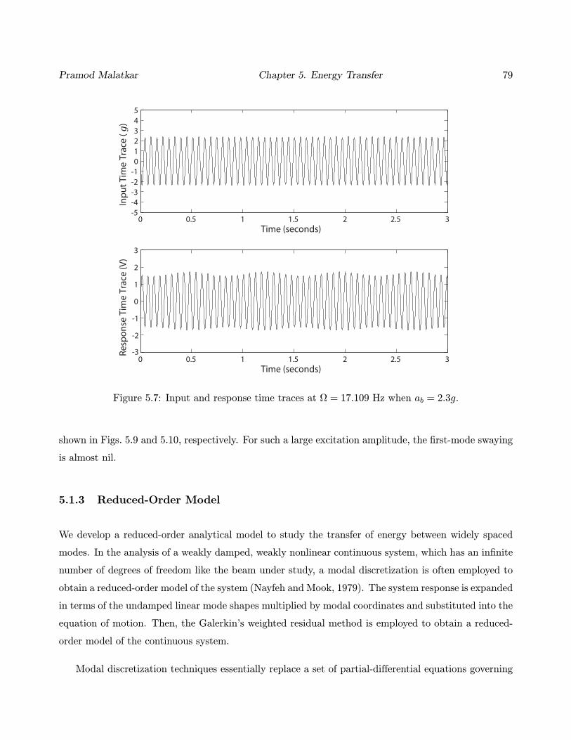
Pramod Malatkar Chapter 5. Energy Transfer 79
0 0.5 1 1.5 2 2.5 3-5-4-3-2-1012345
Time (seconds)
Inpu
t Tim
e Tr
ace
(g)
0 0.5 1 1.5 2 2.5 3 -3
-2
-1
0
1
2
3
Time (seconds)
Resp
onse
Tim
e Tr
ace
(V)
Figure 5.7: Input and response time traces at Ω = 17.109 Hz when ab = 2.3g.
shown in Figs. 5.9 and 5.10, respectively. For such a large excitation amplitude, the first-mode swaying
is almost nil.
5.1.3 Reduced-Order Model
We develop a reduced-order analytical model to study the transfer of energy between widely spaced
modes. In the analysis of a weakly damped, weakly nonlinear continuous system, which has an infinite
number of degrees of freedom like the beam under study, a modal discretization is often employed to
obtain a reduced-order model of the system (Nayfeh and Mook, 1979). The system response is expanded
in terms of the undamped linear mode shapes multiplied by modal coordinates and substituted into the
equation of motion. Then, the Galerkin’s weighted residual method is employed to obtain a reduced-
order model of the continuous system.
Modal discretization techniques essentially replace a set of partial-differential equations governing

Pramod Malatkar Chapter 5. Energy Transfer 80
0 5 10 15 20 2510
-4
10 -3
10 -2
10 -1
100
101
Frequency (Hz)
Inpu
t FFT
0 5 10 15 20 2510
-3
10 -2
10 -1
100
101
Frequency (Hz)
Resp
onse
FFT
Figure 5.8: Input and response FFTs at Ω = 17.109 Hz when ab = 2.3g.
a continuous (infinite-dimensional) system with a finite set of nonlinearly coupled, ordinary-differential
equations in terms of the modal coordinates. For simplicity and faster computation, a minimum
number of modes necessary to represent the response are included in the expansion. However, one
should ensure that the neglected modes do not affect the response of the system significantly, else the
discretized system would lead to erroneous results.
Equations (2.58) and (2.59) governing the nonplanar dynamics of an isotropic, inextensional beam
are simplified to the case of planar motion of a uniform metallic cantilever beam under external exci-
tation. Thus, the governing equation reduces to
mv + cvv +EIviv = mab cosΩt+mg[(s− l)v + v ]−EI v (v v ) − 1
2m v
s
l
∂2
∂t2
s
0v2ds ds
(5.1)

Pramod Malatkar Chapter 5. Energy Transfer 81
0 0.5 1 1.5 2 2.5 3-5-4-3-2-1012345
Time (seconds)
Inpu
t Tim
e Tr
ace
(g)
0 0.5 1 1.5 2 2.5 3 -3
-2
-1
0
1
2
3
Time (seconds)
Resp
onse
Tim
e Tr
ace
(V)
Figure 5.9: Input and response time traces at Ω = 17.547 Hz when ab = 2.97g.
and the associated boundary conditions are
v = 0 and v = 0 at s = 0 (5.2)
v = 0 and v = 0 at s = l (5.3)
The overdot and prime indicate the derivatives with respect to time t and arclength s, respectively,
v(s, t) is the transverse displacement, m is the mass per unit length, l is the beam length, E is Young’s
modulus, I is the area moment of inertia, ab is the acceleration of the supported end (base) of the
beam, g (= 9.8 m/s2) denotes the acceleration due to gravity, cv is the coefficient of linear viscous
damping per unit length, and Ω is the excitation frequency.
In Eq. (5.1), the first of the nonlinear terms on the right-hand side is a hardening nonlinearity
arising from the potential energy stored in bending and is referred to as geometric nonlinearity. The
second nonlinear term is a softening nonlinearity arising from the kinetic energy of axial motion and is
usually referred to as inertia nonlinearity. For the third mode, the inertia nonlinearity is the dominant

Pramod Malatkar Chapter 5. Energy Transfer 82
0 5 10 15 20 2510
-4
10 -3
10 -2
10 -1
100
101
Frequency (Hz)
Inpu
t FFT
0 5 10 15 20 2510
-3
10 -2
10 -1
100
101
Frequency (Hz)
Resp
onse
FFT
Figure 5.10: Input and response FFTs at Ω = 17.547 Hz when ab = 2.97g.
nonlinear term, whereas for the first mode, the geometric nonlinearity is the dominant nonlinear term.
The natural frequencies of the linear system corresponding to Eq. (5.1) are given by ωn = r2n EI/ml4,
where rn is the nth root of the characteristic equation 1+ cos(r) cosh(r) = 0. We introduce nondimen-
sional variables, denoted by an asterisk, by using l as the characteristic length and the inverse of the
third natural frequency ω3 (= 16.824 Hz) as the characteristic time. Then, in nondimensional form,
the governing equation and boundary conditions become
v + µv +1
r43viv = F cosΩt+G[(s− 1)v + v ]− 1
r43v (v v ) − 1
2v
s
1
∂2
∂t2
s
0v2ds ds (5.4)
v = 0 and v = 0 at s = 0 (5.5)
v = 0 and v = 0 at s = 1 (5.6)
where the asterisks have been dropped for ease of notation, F = mab/γ and G = mg/γ with γ =
EIr43/l3 and µ = l2cv/r
23
√mEI. With the chosen nondimensionalization, ω3 = 1 and ω1 = r21/r
23 =
0.057. These frequency values indicate that the third and first modes are widely spaced.

Pramod Malatkar Chapter 5. Energy Transfer 83
As the beam constitutes a weakly nonlinear system, we expand its response v(s, t) in terms of its
undamped linear mode shapes as follows:
v(s, t) =N
i=1
ui(t)φi(s) (5.7)
where N denotes the number of retained modes, the ui(t) are generalized (modal) coordinates, and the
φi(s) denote the normalized undamped linear mode shapes given by
φi(s) = cosh ris− cos ris+ cos ri + cosh risin ri + sinh ri
(sin ris− sinh ris) (5.8)
Substituting Eq. (5.7) into Eq. (5.4), multiplying by φn, integrating the result over the length of the
beam, and using the orthonormal properties of the linear mode shapes yields the set of equations
un + µnun + ω2nun = fn cosΩt +i
gniui +i,j,k
Λnijkuiujuk
+i,j,k
Γnijkuk(uiuj + 2uiuj + uiuj), n = 1, 2, . . . , N (5.9)
where
Λnijk =1
r43
1
0φnφi(φjφk + φjφk )ds
and
Γnijk = −12
1
0
s
0φnφkds
s
0φiφjds ds
are the coefficients of the cubic geometric and inertia nonlinearity terms, respectively, in the discretized
equations, and
µn =1
0µφ2nds, fn =
1
0Fφnds, gni =
1
0Gφn (s− 1)φi + φi ds,
i,j,k
≡i j k
Using cv = 2mζnωexn , where ζn is the damping factor of the nth mode and ω
exn is the experimentally
determined nth natural frequency, we obtain
µn = 2ζnr2nr23
ωexnωn
In the experiments, we observed, during the energy transfer, that the response spectrum consists
essentially of peaks near the first and third natural frequencies (refer to Fig. 5.4), with sidebands around

Pramod Malatkar Chapter 5. Energy Transfer 84
the latter. It is thus natural to include only the third and first modes in the expansion in Eq. (5.7).
But we found out that not including the second and fourth modes led to results inconsistent with the
experimental observations. We, therefore, retain the first four modes in the expansion of v(s, t); that
is, N = 4. Some nonlinear terms in the discretized equations contain un in addition to un and un,
as seen in Eq. (5.9). Solving the four discretized equations for un (n = 1, 2, 3, 4) in terms of un, un,
and t, and using the state-space approach, we obtain the set of eight first-order ordinary-differential
equations
x = F (x, t) (5.10)
where
x = x1, x2, x3, x4, x5, x6, x7, x8T = u1, u1, u2, u2, u3, u3, u4, u4T
and
F (x, t) = x2, u1(x, t), x4, u2(x, t), x6, u3(x, t), x8, u4(x, t)T
The set of first-order ODEs can be easily solved using the following algorithms: Runge-Kutta-Fehlberg
or Adams for non-stiff systems and Gear for stiff systems. But the system of equations is stiff, as the
first mode evolves on a slow scale while the third mode evolves on a fast scale. Thus, the Gear algorithm
would be ideal for solving the system of equations given by Eq. (5.10). Once we know the steady-state
values of the ui, we can substitute them into Eq. (5.7) and determine the transverse displacement v of
the beam.
5.1.4 Numerical Results
We now present results obtained by integrating the set of Eq. (5.10). Figure 5.11 shows the time trace of
the displacement of the beam, at the location where the strain gage is mounted, and the corresponding
FFT at the excitation frequency Ω = 0.977 (= 16.429 Hz) for the excitation amplitude ab = 1.5g. From
the FFT and the time trace, it is obvious that the third-mode response is modulated and that there is
a first-mode component in the response. The modulation frequency (i.e., the sideband spacing) is equal
to the newly created Hopf bifurcation frequency, which is equal to 0.592 Hz. This is, therefore, similar
to the energy transfer observed earlier in the experiments. Also, it is evident from the time trace that
there is a static component present in the displacement v. This is similar to the results obtained by

Pramod Malatkar Chapter 5. Energy Transfer 85
S. Nayfeh and Nayfeh (1993) using their representative model. Keeping the excitation amplitude ab
fixed and lowering the excitation frequency Ω to 0.945 leads to a chaotically modulated motion. The
associated time trace of the displacement and its FFT are shown in Fig. 5.12. Akin to the experimental
results, we see, in the FFT, a peak near the second-mode frequency.
0 50 100 150 200 250 300 350 400 450 500-6
-4
-2
0
2
4
6x 10
-3
Time,
Dis
plac
emen
t,
0 5 10 15 20 2510
-5
10 -4
10 -3
10 -2
Frequency (Hz)
FFT
v
t
Figure 5.11: Displacement time trace and FFT at Ω = 0.977 when ab = 1.5g.
To study the effect of the excitation amplitude ab on the modulation frequency and thus the energy
transfer from the third mode to the first mode, we integrated Eq. (5.10) for three different values of
ab, namely, 1g, 2g, and 2.5g. The corresponding Hopf bifurcation frequencies are found to be 0.571,
0.609, and 0.627 Hz, respectively. The response FFTs are shown in Fig. 5.13. Thus, with an increase
in the excitation amplitude, the analytical model predicts a nominal increase in the Hopf bifurcation
frequency. Whereas in the experiments, the increase in the Hopf bifurcation frequency with an increase
in the excitation amplitude is substantial. Also, the model predicts that the amplitude of the first-mode
component increases with an increase in the excitation amplitude. This is in contradiction with the
trend observed in the experiments.

Pramod Malatkar Chapter 5. Energy Transfer 86
0 100 200 300 400 500 600 700 800 900 1000-0.01
-0.005
0
0.005
0.01
Time,
Dis
plac
emen
t, v
0 5 10 15 20 2510
-6
10 -5
10 -4
10 -3
10 -2
Frequency (Hz)
FFT
t
Figure 5.12: Displacement time trace and FFT at Ω = 0.945 when ab = 1.5g.
5.2 Nonplanar Motion
5.2.1 Experiments with a Circular Rod
In experiments with a slender, circular cross-section, steel, cantilever beam, S. Nayfeh and Nayfeh
(1994) observed the transfer of energy between widely spaced modes via modulation when the rod was
transversely excited near the natural frequency of its fifth (in fact third or any higher) mode. Here we
briefly talk about those experiments and the results obtained by S. Nayfeh and Nayfeh. The length
and diameter of the cantilever, used in the experiments, are 34.5 in and 0.0625 in, respectively, and
its first five linear natural frequencies are 1.303, 9.049, 25.564, 50.213, and 83.150 Hz. The ratio of the
natural frequencies of the first and fifth in-plane (or out-of-plane) modes is around 1:64. Because of
axial symmetry, one-to-one internal resonances occur at each natural frequency of the beam, and the
mode in the plane of excitation interacts with the out-of-plane mode of equal frequency, resulting in
nonplanar whirling motions. For a certain range of parameters, a large-amplitude first-mode response
was accompanied by a modulation of the amplitude and phase of the fifth-mode response, with the
modulation frequency being approximately equal to the natural frequency of the first mode.
The frequency-response curves for the fifth in-plane and out-of-plane modes of the circular rod are

Pramod Malatkar Chapter 5. Energy Transfer 87
0 5 10 15 20 2510
-5
10 -4
10 -3
10 -2
Frequency (Hz)
FFT
0 5 10 15 20 2510
-5
10 -4
10 -3
10 -2
Frequency (Hz)
FFT
0 5 10 15 20 2510
-5
10-4
10 -3
10 -2
Frequency (Hz)
FFT
(a)
(b)
(c)
Figure 5.13: Displacement FFTs at (a) Ω = 0.984 when ab = 1g, (b) Ω = 0.972 when ab = 2g, and (c)
Ω = 0.9678 when ab = 2.5g.
shown in Fig. 5.14. The excitation level was held constant at 2g rms and the excitation frequency
was varied in the neighborhood of the fifth natural frequency. The data in the plots is a composite of
the responses obtained by performing both backward and forward frequency sweeps. In the following

Pramod Malatkar Chapter 5. Energy Transfer 88
paragraphs, we discuss in more detail both the weakly- and strongly-modulated motions observed
during the sweeps.
Figure 5.14: Frequency-response curves of the fifth mode of a circular rod for an excitation amplitude
of 2g rms (S. Nayfeh and Nayfeh, 1994).
The observed weakly-modulated responses contained a large low-frequency component superim-
posed on a nearly constant amplitude fifth-mode whirling motion. Typical short and long time traces

Pramod Malatkar Chapter 5. Energy Transfer 89
Figure 5.15: A short portion of the long time history of a typically weakly modulated motion of a
circular rod (S. Nayfeh and Nayfeh, 1994).
Figure 5.16: Time traces of a typically weakly modulated motion of a circular rod (S. Nayfeh and
Nayfeh, 1994).

Pramod Malatkar Chapter 5. Energy Transfer 90
Figure 5.17: Power spectrum of a typically weakly modulated motion of a circular rod (S. Nayfeh and
Nayfeh, 1994).
of in-plane and out-of-plane responses of this type are shown in Figs. 5.15 and 5.16. The long time
traces illustrate the extremely slow variation of the amplitude of the first mode, but the short time
traces do not readily reveal any modulation of the high-frequency component of the response. A typical
FFT of this type of response is shown in Fig. 5.17. The FFT shows two main peaks, one at the fre-
quency of excitation (near the fifth natural frequency) and the other close to the natural frequency of
the first mode. Sidebands around the peak corresponding to the fifth mode indicate that the response
of the fifth mode is modulated. Moreover, the sideband spacing is close to the first natural frequency.
As indicated by the dense set of sidebands clustered around the peak near the first natural frequency,
the response of the first mode is also modulated.
The most obvious feature of the strongly-modulated motions is the modulation of the amplitude
of the fifth mode. Typical short and long time traces of this type of motion are shown in Figs. 5.18
and 5.19. In constrast to the case of the weakly-modulated motions of Fig. 5.15, the modulation
of the fifth mode is clearly distinguishable in Fig. 5.18. The erratic behavior of the rod response in
Fig. 5.19 suggests that the fifth mode is chaotically modulated, which can be clearly seen by the narrow
band of response present in the neighborhood of the fifth natural frequency in the corresponding FFT
shown in Fig. 5.20. As in the case of the weakly-modulated motions, there appears a dense set of

Pramod Malatkar Chapter 5. Energy Transfer 91
sidebands clustered about the first-natural frequency peak, indicating that the first-mode response is
also modulated.
Figure 5.18: A short portion of the long time history of a typically strongly modulated motion of a
circular rod (S. Nayfeh and Nayfeh, 1994).
Figure 5.19: Time traces of a typically strongly modulated motion of a circular rod (S. Nayfeh and
Nayfeh, 1994).

Pramod Malatkar Chapter 5. Energy Transfer 92
Figure 5.20: Power spectrum of a typically strongly modulated motion of a circular rod (S. Nayfeh and
Nayfeh, 1994).
5.2.2 Reduced-Order Model
Now we develop a reduced-order analytical model to study the transfer of energy between widely spaced
modes via modulation in the presence of a one-to-one internal resonance. This time the out-of-plane
beam motion will also be included in the model. Equations (2.58) and (2.59) governing the nonplanar,
nonlinear dynamics of isotropic, inextensible, Euler-Bernoulli beams will be used to study the response
of the uniform, circular cross-section, metallic cantilever rod used by S. Nayfeh and Nayfeh (1994) in
their experiments. We introduce nondimensional variables, denoted by an asterisk, by using l as the
characteristic length and the inverse of the fifth natural frequency ω5 (= 83.086 Hz) as the characteristic
time. Then, in nondimensional form, the governing equations and boundary conditions become
v + µvv +1
r45viv = F cosΩt+G[(s− 1)v + v ]− 1
r45v (v v ) + v (w w )
−12
vs
1
∂2
∂t2
s
0(v
2+w
2)ds ds (5.11)
w + µww +1
r45wiv = G[(s− 1)w + w ]− 1
r45w (w w ) + w (v v )
−12
ws
1
∂2
∂t2
s
0(v
2+ w
2)ds ds (5.12)

Pramod Malatkar Chapter 5. Energy Transfer 93
v = 0, v = 0, w = 0, and w = 0 at s = 0 (5.13)
v = 0, v = 0, w = 0, and w = 0 at s = 1 (5.14)
where the asterisks have been dropped for ease of notation, F = mab/γ and G = mg/γ with γ =
EIr45/l3, µv = l
2cv/r25
√mEI and µw = l
2cw/r25
√mEI. With the chosen nondimensionalization, ω5 = 1
and ω1 = r21/r25 = 0.0176. These frequency values indicate that the fifth and first modes are widely
spaced.
As the beam constitutes a weakly nonlinear system, we expand its in-plane and out-plane responses,
v(s, t) and w(s, t), in terms of its undamped linear mode shapes as follows:
v(s, t) =i
vi(t)φi(s) (5.15)
w(s, t) =i
wi(t)φi(s) (5.16)
where the vi(t) and wi(t), i = 1, 5, are generalized (modal) coordinates and the φi(s) denote the
normalized undamped linear mode shapes given by Eq. (5.8). We have included only two modes, in
each expansion, to keep the model simple.
Substituting Eqs. (5.15) and (5.16) into Eqs. (5.11) and (5.12), multiplying by φn, integrating the
result over the length of the beam, and using the orthonormal properties of the linear mode shapes
yields the set of equations
vn + µvnvn + ω2nvn = fn cosΩt +i
gnivi +i,j,k
Λnijk(vivjvk + viwjwk)
+i,j,k
Γnijkvk(vivj + 2vivj + vivj + wiwj + 2wiwj + wiwj), n = 1, 5 (5.17)
wn + µwnwn + ω2nwn =i
gniwi +i,j,k
Λnijk(wivjvk + wiwjwk)
+i,j,k
Γnijkwk(vivj + 2vivj + vivj + wiwj + 2wiwj + wiwj), n = 1, 5 (5.18)
where
Λnijk =1
r45
1
0φnφi(φjφk + φjφk )ds
and
Γnijk = −12
1
0
s
0φnφkds
s
0φiφjds ds

Pramod Malatkar Chapter 5. Energy Transfer 94
are the coefficients of the cubic geometric and inertia nonlinearity terms, respectively, in the discretized
equations, and
µvn =1
0µv φ
2nds, µwn =
1
0µw φ
2nds, fn =
1
0Fφnds, gni =
1
0Gφn (s− 1)φi + φi ds
Using cv = 2mζvnωexn and cw = 2mζwnω
exn , where ζvn and ζwn are the damping factors of the nth
in-plane and out-of-plane modes, respectively, and ωexn is the experimentally determined nth natural
frequency, we obtain
µvn = 2ζvnr2nr25
ωexnωn
and µwn = 2ζwnr2nr25
ωexnωn
Some nonlinear terms in the discretized equations contain vn and wn in addition to vn, wn, vn,
and wn. Solving the four discretized equations for vn and wn (n = 1, 5) in terms of vn, wn, vn, wn,
and t, and using the state-space approach, we obtain the set of eight first-order ordinary-differential
equations
x = F (x, t) (5.19)
where
x = x1, x2, x3, x4, x5, x6, x7, x8T = v1, v1, v5, v5, w1, w1, w5, w5T
and
F (x, t) = x2, v1(x, t), x4, v5(x, t), x6, w1(x, t), x8, w5(x, t)T
We integrate Eq. (5.19) for a long time to determine the steady-state values of the vi and wi (i = 1, 5).
Once we know the values of the vi and wi, we can substitute them into Eqs. (5.15) and (5.16) and
determine the in-plane and out-of-plane transverse displacements of the beam; that is, v and w.
5.2.3 Numerical Results
We now present results obtained by integrating the set of Eq. (5.19). We keep the excitation amplitude
ab constant at 2g rms and vary the excitation frequency Ω around the fifth natural frequency ω5. The
values used for the various parameters appearing in the equations are as follows: damping factors
ζv1 = ζw1 = 7.5 10−5 and ζv5 = ζw5 = 2.5 10−3; elasticity modulus E = 200 GPa; and density

Pramod Malatkar Chapter 5. Energy Transfer 95
0 100 200 300 400 500 600 700 800 900 1000
-2
-1
0
1
2
0 100 200 300 400 500 600 700 800 900 1000
-3
-2
-1
0
1
2
3
w (
in m
m)
Time, t
v (
in m
m)
Figure 5.21: Time traces of in-plane and out-of-plane motion of beam at Ω = 82.75 Hz.
ρ = 7830 kg/m3. Figure 5.21 shows the time traces of the in-plane and out-of-plane displacements
of the beam tip at the excitation frequency Ω = 82.75 Hz and the corresponding FFTs are shown in
Fig. 5.22. From the FFTs shown in Fig. 5.22, it is clear that the fifth-mode response is modulated and
that there is a first-mode component in the response. The modulation frequency (i.e., the sideband
spacing) is equal to 1.3 Hz, which is close to the first natural frequency (= 1.303 Hz). But the amplitude
of the first-mode component is very small in comparison to that of the fifth mode, which is apparent
from the time traces and FFTs. This motion is qualitatively similar to the weakly modulated motion
found experimentally by S. Nayfeh and Nayfeh (1994).
Reducing the excitation frequency resulted in a chaotically modulated motion. The time traces
and FFTs of such a motion at Ω = 82.59 Hz are shown in Figs. 5.23 and 5.24, respectively. From the
FFTs, it is clear that both the first and fifth-mode responses are chaotically modulated. This motion is
qualitatively similar to the strongly modulated motion found experimentally by S. Nayfeh and Nayfeh
(1994).

Pramod Malatkar Chapter 5. Energy Transfer 96
0 10 20 30 40 50 60 70 80 90 100
10
10 -2
100
0 10 20 30 40 50 60 70 80 90 100
10 -4
10
100
v
w
Ω (in Hz)
-2
-4
Figure 5.22: FFTs of in-plane and out-of-plane motion of beam at Ω = 82.75 Hz.
5.3 Closure
We observed experimentally that the transfer of energy between widely spaced modes is a function of
the closeness of the modulation frequency to the natural frequency of the first mode. The modulation
frequency, which depends on various parameters like the amplitude and frequency of excitation, damp-
ing factors, etc., has to be near the natural frequency of the first mode for significant transfer of energy
from the directly excited high-frequency third mode to the low-frequency first mode. In such a case,
visually we see a large swaying of the beam due to the large amplitude of the first-mode component in
the beam response. This is akin to primary resonance in a structural system where the closeness of an
external excitation frequency to one of its natural frequencies dictates the magnitude of the structure
response. When the excitation frequency is close to a natural frequency of the structure, the structure
vibrates with a large amplitude, otherwise the amplitude is small.
Using the planar reduced-order model for the rectangular beam, we demonstrated the transfer of
energy from the high-frequency third mode to the low-frequency first mode. Also, we found out that the

Pramod Malatkar Chapter 5. Energy Transfer 97
0 200 400 600 800 1000 1200 1400 1600 1800 2000-4
-2
0
2
4
6
0 200 400 600 800 1000 1200 1400 1600 1800 2000-4
-2
0
2
4
Time, t
w (
in m
m)
v (
in m
m)
Figure 5.23: Time traces of in-plane and out-of-plane motion of beam at Ω = 82.59 Hz.
first four modes need to be included in the Galerkin discretization for accurate modeling of the beam
system. This shows that care should be taken while deciding on the number of modes to be retained
in the approximation. The discrepancy in the experimental and analytical results can be attributed to
a couple of shortcomings in the analytical model. Firstly, the out-of-plane motion is not accounted for
in the model. In the experiments, a small out-of-plane motion is observed. Also, the natural frequency
of the first out-of-plane mode is 22.14 Hz, which is somewhat close to the values used for the excitation
frequency Ω. Therefore, including the out-of-plane motion in the analytical model might lead to better
results. Secondly, the initial curvature in the beam might produce quadratic nonlinearities, which need
to be included in the analytical model.
Using the nonplanar reduced-order model for the circular rod, we demonstrated the transfer of
energy from the high-frequency fifth mode to the low-frequency first-mode in the presence of a one-
to-one internal resonance. The model was able to predict results qualitatively similar to the weakly
and strongly modulated motions observed experimentally by S. Nayfeh and Nayfeh (1994). But the

Pramod Malatkar Chapter 5. Energy Transfer 98
0 10 20 30 40 50 60 70 80 90 100
10-4
10 -2
100
0 10 20 30 40 50 60 70 80 90 100
10 -4
10 -2
100
v
w
Ω (in Hz)
Figure 5.24: FFTs of in-plane and out-of-plane motion of beam at Ω = 82.59 Hz.
reduced-order model predicted, for the amplitude of the first-mode component, values much smaller
than those observed experimentally. To increase the amplitude of the first-mode component, we tried
varying the damping factors, but in vain. This points to some inadequacies in the model. Issues, like
the shaker-structure interaction, nonlinear damping, initial curvature of the beam, extension of the
beam axis, and inclusion of more modes in the modal discretization, were ignored while developing the
model. It is possible that one or more of these factors might be playing a bigger role than expected.
In addition, we also tried to obtain approximate analytical solutions for the beam response using
two perturbation techniques, namely the methods of multiple scales and averaging. Using these two
methods, we could not even demonstrate the transfer of energy from a high-frequency to a low-frequency
mode via modulation. Further investigation needs to be carried out to determine the cause of such a
discrepancy.

Chapter 6
Experiments with a Cantilever Plate
Like beams, rectangular plates are also one of the most commonly used structures in engineering
applications. Many experimental studies have been done so far on rectangular plates, both metallic
and composite, and a variety of nonlinear phenomena observed (Yamaki and Chiba, 1983; Yamaki,
Otomo, and Chiba, 1983; Cole, 1990; Ostiguy and Evan-Iwanowski, 1993; Oh, 1994; Oh and Nayfeh,
1998). For a detailed review of the nonlinear vibration of plates, we refer the reader to Nayfeh and
Mook (1979), Chia (1980), Sathyamoorthy (1997), and Nayfeh (2000).
In this chapter, an experimental study of the response of a thin, rectangular, aluminum cantilever
plate under transverse harmonic excitation is presented. Three test sequences, each involving a fre-
quency sweep around a particular natural frequency of the plate and a different amplitude of base
excitation, are performed. A couple of interesting nonlinear dynamics phenomena present themselves
in every test sequence. These phenomena include two-to-one and three-to-one internal resonances, ex-
ternal combination resonance, energy transfer between widely spaced modes, period-doubled motions,
and chaos. In addition, the influence of the excitation amplitude on the energy transfer between widely
spaced modes via modulation is also investigated.
99

Pramod Malatkar Chapter 6. Cantilever Plate 100
6.1 Test Setup
A schematic of the experimental setup is shown in Fig. 6.1. The uniform cross-section, cantilever
aluminum plate has dimensions 9 × 7.5 × 0.03 (22.86 cm × 19.05 cm × 0.08 cm). The plate is
clamped in a horizontal position to a 2000-lb shaker that provides an external (i.e., transverse to the
plane of the plate) harmonic excitation at the fixed edge of the plate. The plate is not perfectly straight,
but has some initial curvature. The difference in height of the clamped edge and the opposite free edge
of the plate is around 0.4 (1 cm). The shaker excitation is monitored by means of an accelerometer
placed on the clamping fixture, and the response of the cantilever plate is measured using two strain
gages mounted approximately 0.25 (0.64 cm) from the fixed edge and at distances 2.25 (5.72 cm)
and 3.75 (9.53 cm) from the lower left corner of the plate. If a strain gage is located along a nodal
line of a mode, then it would not detect that mode at all. To avoid such a situation, we used two
strain gages and compared, during every reading, their data to ensure that the contributions of all of
the participating modes were being accounted. The signals of the accelerometer and strain gages are
monitored, in both the frequency and time domains, by a digital signal analyzer, which is also used
to drive the shaker. At points of interest, the time- and frequency-response data are stored onto a
floppy disk for further characterization and processing. We waited for a long time to ensure steady
state before taking any measurement. The strain gages basically measure the strain at the location
Figure 6.1: Experimental setup.

Pramod Malatkar Chapter 6. Cantilever Plate 101
where they are mounted on the plate. However, it is difficult to accurately determine the displacement
amplitudes of the various modes from the outputs of the strain-gage conditioners, which are in volts,
especially when there is a modal interaction. Therefore, all of the plots and FFTs are obtained using
strain values only. However, we note that there is no one-to-one correspondence between the strain
values and the displacement amplitudes of the various modes; that is, one strain value could lead to
different displacements for different modes.
A rough estimate of the natural frequencies of the plate was first obtained using the bump test. The
plate was hit by a hammer and an estimate of the natural frequencies was obtained from the peaks in
the subsequent frequency spectra. The peak-hold feature of the signal analyzer was used and an average
from multiple readings was taken for each natural frequency. Later a sweep test around those averaged
values was done to determine the exact natural frequencies. The first seven natural frequencies ωi of
the plate were found to be equal to 17.19 (first bending), 37.75 (first torsional), 110.06, 144.38, 155.56,
291.94, and 302.06 Hz. It is clearly evident that a few natural frequencies are nearly commensurate
with other frequencies or a combination of some of them. So, we can expect some internal resonances
to occur during a sweep of the excitation frequency around those natural frequencies.
6.2 Results
We performed three different frequency sweeps while keeping the value of the base excitation amplitude
ab fixed during each of those sweeps. In the first run, the excitation amplitude was held constant at
2.7g, while the excitation frequency Ω was varied around ω1 + ω7. In the second run, the excitation
frequency was varied around ω7 with ab = 4.5g, and in the final run, a frequency sweep was made
around ω3 keeping the excitation amplitude fixed at 2g. Here, g (= 9.8 m/s2) denotes the acceleration
due to gravity. For all the runs, we present the response frequency spectrum, and in some cases the
input spectrum, response time trace, a pseudo-phase plane, or a Poincare section is also presented.
The frequency spectra of the signals obtained from the accelerometer and strain gages are calculated
in real time using a flat-top window for the first two runs and a Hanning window for the third run.

Pramod Malatkar Chapter 6. Cantilever Plate 102
6.2.1 RUN I: External Combination and Two-to-One Internal Resonances
While doing a backward frequency sweep, starting at Ω = 317 Hz, we observed that the plate response
changed from a periodic response with frequency Ω to one involving three distinct frequencies. The
input and response frequency spectra at Ω = 316.81 Hz are shown in Fig. 6.2. Basically there is a
peak at the excitation frequency Ω and also near the two natural frequencies ω1 (= 17.19 Hz) and ω7
(= 302.06 Hz). Therefore, this is an example of an external combination resonance of the additive type
(Ω ≈ ω1 + ω7), which occurs in the presence of quadratic nonlinearities. But it is well known that the
nonlinearities present in the governing equations of an isotropic cantilever plate are cubic. We suspect
that the initial curvature in the plate could be the cause of the quadratic nonlinearities present in the
system. From Fig. 6.2, it is clear that the peaks at the natural frequencies ω1 and ω7 are much larger
than the one at the excitation frequency Ω, with the peak at ω1 being the largest. The large-amplitude
first-mode response is also visible in the corresponding response time trace shown in Fig. 6.3. Thus,
the external combination resonance has resulted in a transfer of energy from a low-amplitude, high-
frequency mode to a high-amplitude, low-frequency mode. We note that a large static component is
present in the plate responses as seen in the response spectrum (Fig. 6.2) and response time trace
(Fig. 6.3). The cause for this large static component is the improper balancing of the Wheatstone
bridges used in the measurement of the strain values.
In addition, we also obtained a Poincare section using the two strain-gage signals as independent
“pseudo” states (Nayfeh and Balachandran, 1995; Moon, 1987). Poincare section is a powerful geo-
metric tool used to analyze the dynamics of a system. Also, since the dynamics in a state space
reconstructed from scalar time signals not representing displacement or velocity, like the strain-gage
signals, is equivalent to the original dynamics, we conveniently use the strain-gage signals to obtain
the Poincare section. The two strain-gage signals were sampled at the excitation frequency Ω, and
the resulting Poincare section is shown in Fig. 6.4. Because the Poincare section is essentially a closed
curve, the plate motion is two-period quasiperiodic. The scatter in the results could be due to noise.
Reducing the excitation frequency further to Ω = 315 Hz resulted in the fourth and fifth modes getting
excited, possibly through two-to-one internal resonances, as shown in Fig. 6.5. In addition to peaks at
Ω, ω1, and ω7, we now also see peaks at ω4 ≈ 12ω7 and ω5 ≈ 1
2ω7. The two-to-one internal resonances
are due to the presence of quadratic nonlinearities in the plate. The corresponding response time trace
is shown in Fig. 6.6. Reducing the excitation frequency Ω gradually to 313.75 Hz resulted in a motion
similar to the one shown in Fig. 6.2, and at Ω = 313.39 Hz, the plate reverted back to the periodic

Pramod Malatkar Chapter 6. Cantilever Plate 103
0 50 100 150 200 250 300 350 40010
−2
10−1
100
101
Excitation Frequency, Ω (Hz)
Inpu
t FF
T (
V)
0 50 100 150 200 250 300 350 400
10−2
10−1
100
Excitation Frequency, Ω (Hz)
Res
pons
e F
FT
(V
)
Figure 6.2: Input and response FFTs for ab = 2.7g and Ω = 316.81 Hz.
motion with frequency Ω. During a forward sweep, we observed a behavior similar to the one seen
during the backward frequency sweep.
6.2.2 RUN II: Two-to-One and Zero-to-One Internal Resonances
In the second run, the excitation amplitude ab was held constant at 4.5g while the excitation frequency Ω
was varied around the seventh natural frequency ω7. During a backward sweep, starting at Ω = 312 Hz,
we observed a two-to-one internal resonance at Ω = 311.22 Hz. The response spectrum at Ω = 311 Hz
is shown in Fig. 6.7. We see a large peak at the excitation frequency Ω and another one at 12Ω, which
is close to the fifth natural frequency ω5. In addition, we also obtained a pseudo-phase plane using the
strain gage-one and accelerometer signals as independent states. The plot displayed in Fig. 6.8 shows a
typical phase-plane trajectory for a system in which the response period is twice that of the excitation,
as in the present case.

Pramod Malatkar Chapter 6. Cantilever Plate 104
0.2 0.25 0.3 0.35 0.4 0.450
0.2
0.4
0.6
0.8
Time (seconds)
Res
pons
e T
ime
Tra
ce (
V)
Figure 6.3: Response time trace for ab = 2.7g and Ω = 316.81 Hz.
0 0.005 0.01 0.015 0.02−0.02
−0.01
0
0.01
0.02
Strain Gage−One Reading
Str
ain
Gag
e−T
wo
Rea
ding
Figure 6.4: Poincare section showing two-period quasiperiodic motion.
As Ω was reduced, the amplitude of the peak near ω5 kept increasing, and at Ω = 305 Hz it
became larger than that of the peak at Ω. At Ω = 304.69 Hz, the response of the fifth and seventh
modes underwent a Hopf bifurcation, with the newly created frequency, also known as the modulation
frequency, being close and slightly higher than the natural frequency of the first mode. Figure 6.9

Pramod Malatkar Chapter 6. Cantilever Plate 105
0 50 100 150 200 250 300 350 40010
−2
10−1
100
101
Excitation Frequency, Ω (Hz)
Inpu
t FF
T (
V)
0 50 100 150 200 250 300 350 400
10−2
10−1
100
Excitation Frequency, Ω (Hz)
Res
pons
e F
FT
(V
)
Figure 6.5: Input and response FFTs for ab = 2.7g and Ω = 315 Hz.
shows the response spectrum at Ω = 304.5 Hz, where the modulation frequency is equal to 17 Hz,
which is close to ω1 (= 17.19 Hz). It is also clear from the figure that the peak near the first mode
frequency ω1 is the largest. Thus, energy was transferred from two high-frequency modes, namely
the fifth and seventh, to the low-frequency first mode via modulation. This is an example of the
energy transfer between widely spaced modes, also known as zero-to-one internal resonance. As Ω was
gradually reduced from 304.69 Hz, the modulation frequency tended to go towards the first natural
frequency and the amplitude of the first-mode response kept increasing. But once the modulation
frequency had passed the first natural frequency, the first-mode response amplitude started decreasing.
At Ω = 304.41 Hz, the plate response reverted back to the periodic motion with frequency Ω. A similar
behavior was observed during a forward sweep of the excitation frequency in the frequency range of
interest.
To study the influence of the excitation amplitude on the modulation frequency and, in turn, on
the first-mode response, we reduced the excitation amplitude to ab = 3g. At Ω = 300.94 Hz, the

Pramod Malatkar Chapter 6. Cantilever Plate 106
0.2 0.25 0.3 0.35 0.4 0.450
0.1
0.2
0.3
0.4
0.5
0.6
0.7
0.8
Time (seconds)
Res
pons
e T
ime
Tra
ce (
V)
Figure 6.6: Response time trace for ab = 2.7g and Ω = 315 Hz.
0 50 100 150 200 250 300 350 400
10−2
10−1
100
Excitation Frequency, Ω (Hz)
Res
pons
e F
FT
(V
)
Figure 6.7: Response FFT for ab = 4.5g and Ω = 311 Hz.
modulation frequency was equal to 11.7 Hz, which is far away from the first natural frequency ω1
(= 17.19 Hz). Hence the amplitude of the first-mode response was very small, as is evident from the
response spectrum shown in Fig. 6.10. A similar trend was observed in Chapter 5 while experimentally
studying the transfer of energy between widely spaced modes in cantilever beams.

Pramod Malatkar Chapter 6. Cantilever Plate 107
0 0.01 0.02 0.03 0.04−0.5
−0.25
0
0.25
0.5
Strain Gage−One Reading
Acc
eler
omet
er R
eadi
ng
Figure 6.8: Pseudo-phase plane trajectory showing two-to-one internal resonance.
0 50 100 150 200 250 300 350 400
10−2
10−1
Excitation Frequency, Ω (Hz)
Res
pons
e F
FT
(V
)
Figure 6.9: Response FFT for ab = 4.5g and Ω = 304.5 Hz.
6.2.3 RUN III: Quasiperiodic Motion and Three-to-One Internal Resonance
This time we did a frequency sweep around the third-mode frequency ω3 (= 110.06 Hz) keeping the
base excitation fixed at 2g. Starting with Ω = 110 Hz and going backward in small increments, we
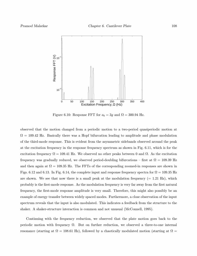
Pramod Malatkar Chapter 6. Cantilever Plate 108
0 50 100 150 200 250 300 350 400
10−2
10−1
Excitation Frequency, Ω (Hz)
Res
pons
e F
FT
(V
)
Figure 6.10: Response FFT for ab = 3g and Ω = 300.94 Hz.
observed that the motion changed from a periodic motion to a two-period quasiperiodic motion at
Ω = 109.42 Hz. Basically there was a Hopf bifurcation leading to amplitude and phase modulation
of the third-mode response. This is evident from the asymmetric sidebands observed around the peak
at the excitation frequency in the response frequency spectrum as shown in Fig. 6.11, which is for the
excitation frequency Ω = 109.41 Hz. We observed no other peaks between 0 and Ω. As the excitation
frequency was gradually reduced, we observed period-doubling bifurcations — first at Ω = 109.39 Hz
and then again at Ω = 109.35 Hz. The FFTs of the corresponding zoomed-in responses are shown in
Figs. 6.12 and 6.13. In Fig. 6.14, the complete input and response frequency spectra for Ω = 109.35 Hz
are shown. We see that now there is a small peak at the modulation frequency (= 1.21 Hz), which
probably is the first-mode response. As the modulation frequency is very far away from the first natural
frequency, the first-mode response amplitude is very small. Therefore, this might also possibly be an
example of energy transfer between widely spaced modes. Furthermore, a close observation of the input
spectrum reveals that the input is also modulated. This indicates a feedback from the structure to the
shaker. A shaker-structure interaction is common and not unusual (McConnell, 1995).
Continuing with the frequency reduction, we observed that the plate motion goes back to the
periodic motion with frequency Ω. But on further reduction, we observed a three-to-one internal
resonance (starting at Ω = 108.61 Hz), followed by a chaotically modulated motion (starting at Ω =

Pramod Malatkar Chapter 6. Cantilever Plate 109
100 105 110 115 12010
−3
10−2
10−1
100
101
Excitation Frequency, Ω (Hz)
Res
pons
e F
FT
(V
)
Figure 6.11: Response FFT for ab = 2g and Ω = 109.41 Hz.
100 105 110 115 12010
−3
10−2
10−1
100
101
Excitation Frequency, Ω (Hz)
Res
pons
e F
FT
(V
)
Figure 6.12: Response FFT for ab = 2g and Ω = 109.39 Hz.
108.5 Hz), followed by a three-to-one internal resonance again (starting at Ω = 108.45 Hz), and then
the usual periodic motion (starting at Ω = 108.39 Hz). The occurrence of the three-to-one internal

Pramod Malatkar Chapter 6. Cantilever Plate 110
100 105 110 115 12010
−3
10−2
10−1
100
101
Excitation Frequency, Ω (Hz)
Res
pons
e F
FT
(V
)
Figure 6.13: Response FFT for ab = 2g and Ω = 109.35 Hz.
resonance is due to the fact that the plate system has inherent cubic geometric nonlinearities and
because ω3 ≈ 3ω2. The response spectra corresponding to the three-to-one internal resonance at
Ω = 108.4 Hz and the chaotically-modulated three-to-one internal resonance at Ω = 108.5 Hz are
shown in Figs. 6.15 and 6.16, respectively. The forward sweep also led to identical motions in the
above frequency range of interest.
6.3 Closure
It is very interesting to see so many nonlinear dynamic phenomena in a simple aluminum plate. The
initial curvature of the plate brought quadratic nonlinearities into the system, which provided an
opportunity to observe phenomena which otherwise would not have occurred in a straight plate with just
cubic nonlinearities. Also, many of the linear natural frequencies of the plate are nearly commensurate
with one another, leading to multiple internal resonances.
The energy transfer from a low-amplitude, high-frequency mode to a high-amplitude, low-frequency
mode via modulation was demonstrated. Also, the amount of energy transfer is found to be strongly
dependent on the closeness of the modulation frequency to the natural frequency of the low-frequency

Pramod Malatkar Chapter 6. Cantilever Plate 111
0 20 40 60 80 100 120
10−2
10−1
100
101
Excitation Frequency, Ω (Hz)
Inpu
t FF
T (
V)
0 20 40 60 80 100 120
10−2
10−1
100
101
Excitation Frequency, Ω (Hz)
Res
pons
e F
FT
(V
)
Figure 6.14: Input and response FFTs for ab = 2g and Ω = 109.35 Hz.
mode. The results of RUN III show that the two-period quasiperiodic motion is due to an instability
involving both the first and third modes. Probably it would not be amiss to generalize that a Hopf
bifurcation in a structure under harmonic excitation would involve at least two modes. Hence, while
trying to explain such a phenomenon analytically, a single-mode approximation should not be used as
it might lead to erroneous results.

Pramod Malatkar Chapter 6. Cantilever Plate 112
0 50 100 150 200
10−2
10−1
100
101
Excitation Frequency, Ω (Hz)
Res
pons
e F
FT
(V
)
Figure 6.15: Response FFT for ab = 2g and Ω = 108.4 Hz.
0 50 100 150 20010
−3
10−2
10−1
100
101
Excitation Frequency, Ω (Hz)
Res
pons
e F
FT
(V
)
Figure 6.16: Response FFT for ab = 2g and Ω = 108.5 Hz.

Chapter 7
Conclusions and Recommendation for
Future Work
7.1 Summary
In this dissertation, we investigated the nonlinear vibrations of metallic cantilever beams and plates
subjected to transverse harmonic excitations. In particular, we studied both experimentally and the-
oretically the energy transfer between widely spaced modes via modulation. Two cases — planar and
nonplanar motions — were considered. In the planar case, a rectangular cross-section beam whose
motion was restricted to the plane of excitation was studied. Whereas in the nonplanar case, a circu-
lar cross-section rod, where because of axial symmetry, one-to-one internal resonances occur at each
natural frequency of the beam, was studied.
Experimentally it was observed that the transfer of energy between widely spaced modes is a
function of the closeness of the modulation frequency to the natural frequency of the first mode.
The modulation frequency, which depends on various parameters like the amplitude and frequency of
excitation, damping factors, etc., has to be near the natural frequency of the first mode for significant
transfer of energy from the directly excited high-frequency third mode to the low-frequency first mode.
In such a case, visually we see a large swaying of the beam due to the large amplitude of the first-mode
component in the beam response. This is very similar to primary resonance in a structural system
113

Pramod Malatkar Chapter 7. Conclusions 114
where the closeness of an external excitation frequency to the natural frequencies of the structure
dictates the magnitude of the structure response.
Based on the present observations, we can conclude that conventional methods used for reduction
of response amplitude, such as decreasing amplitude of excitation or increasing damping, might in
fact lead to an increase in the amplitude of the low-frequency response if they result in bringing the
modulation frequency closer to the first natural frequency. Also, in most of the experiments dealing
with energy transfer via modulation from high- to low-frequency modes, it was observed that the low-
frequency mode is always the first mode. As the modulation frequency (or the newly created frequency)
increases with increasing amplitude of excitation, it might be therefore possible to excite the second
mode, instead of the first, if the forcing amplitude is large enough. However, this needs to be verified
experimentally.
The reduced-order models were able to predict results qualitatively similar to the experimentally
observed motions, but the results differed a lot quantitatively. Issues, like the shaker-structure inter-
action, nonlinear damping, initial curvature of the beam, extension of the beam axis, and inclusion of
more modes in the modal discretization, were ignored while developing the models. It is, therefore,
possible that one or more of these factors might be playing a bigger role than expected, and this needs
to be further investigated.
An experimental parametric identification technique to estimate the linear and nonlinear damping
coefficients and effective nonlinearity of a metallic cantilever beam was also developed. This method
can be applied to any single-degree-of-freedom nonlinear system with weak cubic geometric and inertia
nonlinearities. It was found that noninclusion of quadratic nonlinearity in the beam model might lead
to incorrect parameter estimation. In addition, we proposed two methods, based on the elimination
theory of polynomials, which can be used to determine both the critical forcing amplitude as well as the
jump frequencies in single-degree-of-freedom nonlinear systems. These two methods have the potential
of being applicable to multiple-degree-of-freedom nonlinear systems as well.
Finally, we carried out an experimental study of the response of a rectangular, aluminum cantilever
plate to transverse harmonic excitations. We observed various nonlinear dynamic phenomena, like two-
to-one and three-to-one internal resonances, external combination resonance, energy transfer between
widely spaced modes via modulation, period-doubled motions, and chaos. The fact that a simple
plate under harmonic excitation could display so many different nonlinear dynamic phenomena proves

Pramod Malatkar Chapter 7. Conclusions 115
that nonlinear phenomena are ubiquitous. Some may however remark that these types of nonlinear
resonances have very high activation thresholds; that is, the excitation level needs to be large to
observe them. But since these unusual phenomena have been observed in real engineering structures
and mechanical systems, there is a need to study such phenomena in more detail. For instance, the
zero-to-one internal resonance was observed in the motion of the solar panels of the Hubble space
telescope and also in the motion of the skin of a submarine. Many physical systems display nonlinear
behavior, but only a watchful eye can recognize that. Most of the time our “linear” perspective (or in
other words, our ignorance about nonlinear phenomena) makes us overlook any such different behavior
in systems. It would be to our advantage if we start to think “nonlinearly”.
7.2 Suggestions for Future Work
There is a lot of scope for improvement in the model used for describing the nonlinear, nonplanar
dynamics of an isotropic, cantilever beam. Better models would lead to better agreement, both quali-
tatively and quantitatively, between the predicted and experimental results. Also, such models can be
used to explain the many interesting motions observed experimentally.
Transfer of energy from high- to low-frequency modes is extremely dangerous as the amplitudes of
the low-frequency modes are usually much larger than the directly-excited high-frequency modes. The
strong dependence of the energy transfer between widely spaced modes on the modulation frequency
can be utilized to control the amplitude of the low-frequency responses. Therefore, a study on such a
control technique is highly recommended.
It would be interesting to see if energy transfer between widely spaced modes via modulation also
occurs in micro-electromechanical systems (MEMS). In MEMS-based devices, the forcing term is highly
nonlinear and varies with the displacement of the microstructure. One could study the influence of
such a forcing term on the occurence of the energy transfer between widely spaced modes. Also, the
applicability of the experimental parametric identification technique to estimate the damping factors
and effective nonlinearity in such systems can be studied.

Bibliography
[1] Adams, R. D. and Bacon, D. G. C., Measurement of the flexural damping capacity and dy-
namic Young’s modulus of metals and reinforced plastics, Journal of Physics D: Applied Physics,
6 (1973), pp. 27—41.
[2] Alhazza, K. A. and Nayfeh, A. H., Nonlinear vibrations of doubly-curved cross-ply shal-
low shells, in Proceedings of the 42nd AIAA/ASME/ASCE/AHS/ASC Structures, Structural
Dynamics, and Materials Conference, Seattle, Washington, 2001.
[3] Anand, G. V., Nonlinear resonance in stretched strings with viscous damping, Journal of the
Acoustical Society of America, 40 (1966), pp. 1517—1528.
[4] Anand, G. V., Stability of nonlinear oscillations of stretched strings, Journal of the Acoustical
Society of America, 46 (1969), pp. 667—677.
[5] Anderson, T. J., Balachandran, B., and Nayfeh, A. H., Observations of nonlinear in-
teractions in a flexible cantilever beam, in Proceedings of the 33rd AIAA Structures, Structural
Dynamics, and Materials Conference, Dallas, Texas, 1992, pp. 1678—1686.
[6] Anderson, T. J., Balachandran, B., and Nayfeh, A. H., Nonlinear resonances in a flexible
cantilever beam, Journal of Vibration and Acoustics, 116 (1994), pp. 480—484.
[7] Anderson, T. J., Nayfeh, A. H., and Balachandran, B., Coupling between high-frequency
modes and a low-frequency mode: Theory and experiment, Nonlinear Dynamics, 11 (1996a),
pp. 17—36.
[8] Anderson, T. J., Nayfeh, A. H., and Balachandran, B., Experimental verification of the
importance of the nonlinear curvature in the response of a cantilever beam, Journal of Vibration
and Acoustics, 118 (1996b), pp. 21—27.
116

Pramod Malatkar Bibliography 117
[9] Annigeri, B. S., Cassenti, B. N., and Dennis, A. J., Kinematics of small and large defor-
mations of continua, Engineering Computations, 2 (1985), pp. 247—256.
[10] Arafat, H. N., Nonlinear Response of Cantilever Beams, Ph.D. thesis, Virginia Polytechnic
Institute and State University, Blacksburg, Virginia, 1999.
[11] Arafat, H. N. and Nayfeh, A. H., Transfer of energy from high- to low-frequency modes
in the bending-torsion oscillation of cantilever beams, in Proceedings of the 1999 ASME Design
Engineering Technical Conferences, Las Vegas, Nevada, 1999.
[12] Arafat, H. N. and Nayfeh, A. H., The influence of nonlinear boundary conditions on the
nonplanar autoparametric responses of an inextensible beam, in Proceedings of the 2001 ASME
Design Engineering Technical Conferences, Pittsburgh, Pennsylvania, 2001.
[13] Aravamudan, K. S. and Murthy, P. N., Non-linear vibration of beams with time-dependent
boundary conditions, International Journal of Non-Linear Mechanics, 8 (1973), pp. 195—212.
[14] Atluri, S., Nonlinear vibrations of a hinged beam including nonlinear inertia effects, Journal of
Applied Mechanics, 40 (1973), pp. 121—126.
[15] Bailey, C. D., A new look at Hamilton’s principle, Foundations of Physics, 5 (1975a), pp. 433—
451.
[16] Bailey, C. D., Application of Hamilton’s law of varying action, AIAA Journal, 13 (1975b),
pp. 1154—1157.
[17] Benhafsi, Y., Penny, J. E. T., and Friswell, M. I., Identification of damping parameters
of vibrating systems with cubic stiffness nonlinearity, in Proceedings of the 13th International
Modal Analysis Conference, Nashville, Tennessee, 1995, pp. 623—629.
[18] Bolotin, V. V., The Dynamic Stability of Elastic Systems, Holden-Day, San Francisco, Cali-
fornia, 1964.
[19] Burgreen, D., Free vibrations of a pin-ended column with constant distance between pin ends,
Journal of Applied Mechanics, 18 (1951), pp. 135—139.
[20] Burton, T. D. and Kolowith, M., Nonlinear resonances and chaotic motion in a flexible
parametrically excited beam, in Proceedings of the 2nd Conference on Nonlinear Vibrations, Sta-
bility, and Dynamics of Structures and Mechanisms, Blacksburg, Virginia, 1988.

Pramod Malatkar Bibliography 118
[21] Busby, H. R. and Weingarten, V. I., Non-linear response of a beam to periodic loading,
International Journal of Non-Linear Mechanics, 7 (1972), pp. 289—303.
[22] Caughey, T. K. and O’Kelly, M. E. J., Effect of damping on the natural frequencies of
linear dynamic systems, Journal of the Acoustical Society of America, 33 (1961), pp. 1458—1461.
[23] Chia, C. Y., Nonlinear Analysis of Plates, McGraw-Hill, New York, 1980.
[24] Chun, K. R., Free vibration of a beam with one end spring-hinged and the other free, Journal of
Applied Mechanics, 39 (1972), pp. 1154—1155.
[25] Cole, S. R., Effects of spoiler surfaces on the aeroelastic behavior of a low-aspect-ratio rectan-
gular wing, AIAA Paper 90-0981, 1990.
[26] Cowper, G. R., The shear coefficient in Timoshenko’s beam theory, Journal of Applied Me-
chanics, 33 (1966), pp. 335—340.
[27] Cowper, G. R., On the accuracy of Timoshenko’s beam theory, Journal of the Engineering
Mechanics Division, 94 (1968), pp. 1447—1453.
[28] Cox, D., Little, J., and O’Shea, D., Ideals, Varieties, and Algorithms, Springer-Verlag, New
York, 1997.
[29] Crawley, E. F. and Aubert, A. C., Identification of nonlinear structural elements by force-
state mapping, AIAA Journal, 24 (1986), pp. 155—162.
[30] Crespo da Silva, M. R. M., Flexural-flexural oscillations of Beck’s column subject to a planar
harmonic excitation, Journal of Sound and Vibration, 60 (1978a), pp. 133—144.
[31] Crespo da Silva, M. R. M., Harmonic non-linear response of Beck’s column to a lateral
excitation, International Journal of Solids and Structures, 14 (1978b), pp. 987—997.
[32] Crespo da Silva, M. R. M., On the whirling of a base-excited cantilever beam, Journal of the
Acoustical Society of America, 67 (1980), pp. 704—707.
[33] Crespo da Silva, M. R. M., Non-linear flexural-flexural-torsional-extensional dynamics of
beams. I: Formulation, International Journal of Solids and Structures, 24 (1988a), pp. 1225—
1234.

Pramod Malatkar Bibliography 119
[34] Crespo da Silva, M. R. M., Non-linear flexural-flexural-torsional-extensional dynamics of
beams. II: Response analysis, International Journal of Solids and Structures, 24 (1988b), pp. 1235—
1242.
[35] Crespo da Silva, M. R. M., Equations for nonlinear analysis of 3d motions of beams, Applied
Mechanics Reviews, 44 (1991), pp. S51—S59.
[36] Crespo da Silva, M. R. M. and Glynn, C. C., Nonlinear flexural-flexural-torsional dynamics
of inextensional beams. I: Equations of motion, Journal of Structural Mechanics, 6 (1978a),
pp. 437—448.
[37] Crespo da Silva, M. R. M. and Glynn, C. C., Nonlinear flexural-flexural-torsional dynamics
of inextensional beams. II: Forced motions, Journal of Structural Mechanics, 6 (1978b), pp. 449—
461.
[38] Crespo da Silva, M. R. M. and Glynn, C. C., Out-of-plane vibrations of a beam including
non-linear inertia and non-linear curvature effects, International Journal of Non-Linear Mechan-
ics, 13 (1979a), pp. 261—271.
[39] Crespo da Silva, M. R. M. and Glynn, C. C., Non-linear non-planar resonant oscillations
in fixed-free beams with support asymmetry, International Journal of Solids and Structures, 15
(1979b), pp. 209—219.
[40] Crespo da Silva, M. R. M. and Hodges, D. H., Nonlinear flexure and torsion of rotating
beams, with application to helicopter rotor blades. I: Formulation, Vertica, 10 (1986a), pp. 151—
169.
[41] Crespo da Silva, M. R. M. and Hodges, D. H., Nonlinear flexure and torsion of rotating
beams, with application to helicopter rotor blades. II: Response and stability results, Vertica, 10
(1986b), pp. 171—186.
[42] Crespo da Silva, M. R. M. and Zaretzky, C. L., Non-linear modal coupling in planar and
non-planar responses of inextensional beams, International Journal of Non-Linear Mechanics, 25
(1990), pp. 227—239.
[43] Crespo da Silva, M. R. M. and Zaretzky, C. L., Nonlinear flexural-flexural-torsional in-
teractions in beams including the effect of torsional dynamics. I: Primary resonance, Nonlinear
Dynamics, 5 (1994), pp. 3—23.

Pramod Malatkar Bibliography 120
[44] Crespo da Silva, M. R. M., Zaretzky, C. L., and Hodges, D. H., Effects of approxima-
tions on the static and dynamic response of a cantilever with a tip mass, International Journal
of Solids and Structures, 27 (1991), pp. 565—583.
[45] Cusumano, J. P. and Moon, F. C., Low dimensional behavior in chaotic nonplanar motions
of a forced elastic rod: Experiment and theory, in Nonlinear Dynamics in Engineering Systems,
Schiehlen, W., ed., Springer-Verlag, New York, 1990, pp. 60—66.
[46] Cusumano, J. P. and Moon, F. C., Chaotic non-planar vibrations of the thin elastica. Part
I: Experimental observation of planar instability, Journal of Sound and Vibration, 179 (1995a),
pp. 185—208.
[47] Cusumano, J. P. and Moon, F. C., Chaotic non-planar vibrations of the thin elastica. Part
II: Derivation and analysis of a low-dimensional model, Journal of Sound and Vibration, 179
(1995b), pp. 209—226.
[48] Danielson, D. A. and Hodges, D. H., Nonlinear beam kinematics by decomposition of the
rotation tensor, Journal of Applied Mechanics, 54 (1987), pp. 258—262.
[49] Dokumaci, E., Pseudo-coupled bending-torsion vibrations of beams under lateral parametric
excitation, Journal of Sound and Vibration, 58 (1978), pp. 233—238.
[50] Doughty, T. A., Davies, P., and Bajaj, A. K., A comparison of three techniques using
steady state data to identify non-linear modal behavior of an externally excited cantilever beam,
Journal of Sound and Vibration, 249 (2002), pp. 785—813.
[51] Dowell, E. H., On asymptotic approximations to beam mode shapes, Journal of Applied Me-
chanics, 51 (1984), p. 439.
[52] Dowell, E. H., Traybar, J., and Hodges, D. H., An experimental-theoretical correlation
study of non-linear bending and torsion deformations of a cantilever beam, Journal of Sound and
Vibration, 50 (1977), pp. 533—544.
[53] Dugundji, J., Simple expressions for higher vibration modes of uniform Euler beams, AIAA
Journal, 26 (1988), pp. 1013—1014.
[54] Dugundji, J. and Mukhopadhyay, V., Lateral bending-torsion vibrations of a thin beam under
parametric excitation, Journal of Applied Mechanics, 40 (1973), pp. 693—698.

Pramod Malatkar Bibliography 121
[55] Eisley, J. G., Nonlinear vibration of beams and rectangular plates, ZAMP, 15 (1964), pp. 167—
175.
[56] Emam, S. A. and Nayfeh, A. H., Nonlinear dynamics of a clamped-clamped buckled beam, in
Proceedings of the 43rd AIAA/ASME/ASCE/AHS/ASC Structures, Structural Dynamics, and
Materials Conference, Denver, Colorado, 2002.
[57] Epstein, M. and Murray, D. W., Three-dimensional large deformation analysis of thin walled
beams, International Journal of Solids and Structures, 12 (1976), pp. 867—876.
[58] Evan-Iwanowski, R. M., On the parametric response of structures, Applied Mechanics Reviews,
18 (1965), pp. 699—702.
[59] Evan-Iwanowski, R. M., Resonance Oscillations in Mechanical Systems, Elsevier, New York,
1976.
[60] Evensen, D. A., Nonlinear vibrations of beams with various boundary conditions, AIAA Journal,
6 (1968), pp. 370—372.
[61] Fahey, S. O. and Nayfeh, A. H., Experimental nonlinear identification of a single structural
mode, in Proceedings of the 16th International Modal Analysis Conference, Orlando, Florida,
1998, pp. 737—745.
[62] Feng, Z. C., Nonresonant modal interactions, in Proceedings of the 1995 ASME Design Engi-
neering Technical Conferences, Boston, Massachusetts, 1995, pp. 511—517.
[63] Friswell, M. I. and Penny, J. E. T., The accuracy of jump frequencies in series solutions of
the response of a Duffing oscillator, Journal of Sound and Vibration, 169 (1994), pp. 261—269.
[64] Fung, Y. C., Foundations of Solid Mechanics, Prentice-Hall, Englewood Cliffs, New Jersey,
1965.
[65] Ginsberg, J. H., The effects of damping on a non-linear system with two degrees of freedom,
International Journal of Non-Linear Mechanics, 7 (1972), pp. 323—336.
[66] Gorman, D. J., Free Vibration Analysis of Beams and Shafts, Wiley, New York, 1975.
[67] Griffiths, L. W., Introduction to the Theory of Equations, Wiley, New York, 1947.

Pramod Malatkar Bibliography 122
[68] Haddow, A. G. and Hasan, S. M., Nonlinear oscillation of a flexible cantilever: Experimental
results, in Proceedings of the 2nd Conference on Nonlinear Vibrations, Stability, and Dynamics
of Structures and Mechanisms, Blacksburg, Virginia, 1988.
[69] Haight, E. C. and King, W. W., Stability of parametrically excited vibrations of an elastic
rod, Developments in Theoretical and Applied Mechanics, 5 (1971), pp. 677—713.
[70] Haight, E. C. and King, W. W., Stability of nonlinear oscillations of an elastic rod, Journal
of the Acoustical Society of America, 52 (1972), pp. 899—911.
[71] Haller, G., Chaos Near Resonance, Springer-Verlag, New York, 1999.
[72] Henry, R. F. and Tobias, S. A.,Modes at rest and their stability in coupled non-linear systems,
Journal of Mechanical Engineering Science, 3 (1961), pp. 163—173.
[73] Hinnant, H. E. and Hodges, D. H., Nonlinear analysis of a cantilever beam, AIAA Journal,
26 (1988), pp. 1521—1527.
[74] Ho, C.-H., Scott, R. A., and Eisley, J. G., Non-planar, non-linear oscillations of a beam.
I: Forced motions, International Journal of Non-Linear Mechanics, 10 (1975), pp. 113—127.
[75] Ho, C.-H., Scott, R. A., and Eisley, J. G., Non-planar, non-linear oscillations of a beam.
II: Free motions, Journal of Sound and Vibration, 47 (1976), pp. 333—339.
[76] Hodges, D. H., Finite rotation and nonlinear beam kinematics, Vertica, 11 (1987a), pp. 297—307.
[77] Hodges, D. H., Nonlinear beam kinematics for small strains and finite rotations, Vertica, 11
(1987b), pp. 573—589.
[78] Hodges, D. H., Crespo da Silva, M. R. M., and Peters, D. A., Nonlinear effects in the
static and dynamic behavior of beams and rotor blades, Vertica, 12 (1988), pp. 243—256.
[79] Hodges, D. H. and Dowell, E. H., Nonlinear equations of motion for the elastic bending and
torsion of twisted nonuniform rotor blades, NASA Technical Note D-7818, 1974.
[80] Huang, T. C., The effect of rotatory inertia and of shear deformation on the frequency and nor-
mal mode equations of uniform beams with simple end conditions, Journal of Applied Mechanics,
28 (1961), pp. 579—584.

Pramod Malatkar Bibliography 123
[81] Hughes, G. C. and Bert, C. W., Effect of gravity on nonlinear oscillations of a horizontal,
immovable-end beam, in Proceedings of the 3rd Conference on Nonlinear Vibrations, Stability,
and Dynamics of Structures and Mechanisms, Blacksburg, Virginia, 1990.
[82] Hyer, M. W., Whirling of a base-excited cantilever beam, Journal of the Acoustical Society of
America, 65 (1979), pp. 931—939.
[83] Ibrahim, R. A. and Hijawi, M., Deterministic and stochastic response of nonlinear coupled
bending-torsion modes in a cantilever beam, Nonlinear Dynamics, 16 (1998), pp. 259—292.
[84] Kane, T. R., Ryan, R. R., and Banerjee, A. K., Dynamics of a cantilever beam attached
to a moving base, Journal of Guidance, 10 (1987), pp. 139—151.
[85] Kapania, R. K. and Park, S., Parametric identification of nonlinear structural dynamic sys-
tems using time finite element method, AIAA Journal, 35 (1997), pp. 719—726.
[86] Karman, T. V., The engineer grapples with nonlinear problems, Bulletin of the American Math-
ematical Society, 46 (1940), pp. 615—683.
[87] Krauss, R. W. and Nayfeh, A. H., Comparison of experimental identification techniques for
a nonlinear SDOF system, in Proceedings of the 17th International Modal Analysis Conference,
Santa Barbara, California, 1999a, pp. 1182—1187.
[88] Krauss, R. W. and Nayfeh, A. H., Experimental nonlinear identification of a single mode of
a transversely excited beam, Nonlinear Dynamics, 18 (1999b), pp. 69—87.
[89] Lacarbonara, W., Direct treatment and discretizations of non-linear spatially continuous sys-
tems, Journal of Sound and Vibration, 221 (1999), pp. 849—866.
[90] Langford, W., Normal form analysis of Nayfeh’s abnormal resonance, in Annual Meeting of
the Canadian Applied and Industrial Mathematics Society, Victoria, Canada, 2001.
[91] Lee, G.-M., Estimation of non-linear system parameters using higher-order frequency response
functions, Mechanical Systems and Signal Processing, 11 (1997), pp. 219—228.
[92] Love, A. E. H., A Treatise on the Mathematical Theory of Elasticity, Dover, New York, 1944.
[93] Malatkar, P. and Nayfeh, A. H., Calculation of the jump frequencies in the response of
s.d.o.f. non-linear systems, Journal of Sound and Vibration, 254 (2002), pp. 1005—1011.

Pramod Malatkar Bibliography 124
[94] Malatkar, P. and Nayfeh, A. H., A parametric identification technique for SDOF weakly
nonlinear systems with cubic nonlinearities, Journal of Vibration and Control, 9 (2003a), pp. 317—
336.
[95] Malatkar, P. and Nayfeh, A. H., On the transfer of energy between widely spaced modes in
structures, Nonlinear Dynamics, 31 (2003b), pp. 225—242.
[96] Malatkar, P. and Nayfeh, A. H., A plethora of nonlinear dynamics phenomena observed
in a simple cantilever plate, 2003 ASME Design Engineering Technical Conferences, Chicago,
Illinois, accepted (2003c).
[97] Masri, S. F. and Caughey, T. K., A nonparametric identification technique for nonlinear
dynamic problems, Journal of Applied Mechanics, 46 (1979), pp. 433—447.
[98] Masri, S. F., Sassi, H., and Caughey, T. K., Nonparametric identification of nearly arbitrary
nonlinear systems, Journal of Applied Mechanics, 49 (1982), pp. 619—628.
[99] McConnell, K. G., Vibration Testing: Theory and Practice, Wiley, New York, 1995.
[100] McDaniel, J. G., Widjaja, F., Barbone, P. E., and Pierce, A. D., Estimating natural
frequencies and mode shapes from forced response calculations, AIAA Journal, 40 (2002), pp. 758—
764.
[101] McDonald, P. H., Nonlinear dynamic coupling in a beam vibration, Journal of Applied Me-
chanics, 22 (1955), pp. 573—578.
[102] Meirovitch, L., Analytical Methods in Dynamics, Macmillan, New York, 1967.
[103] Meirovitch, L., Principles and Techniques of Vibrations, Prentice Hall, Upper Saddle River,
New Jersey, 1997.
[104] Miles, J. W., Stability of forced oscillations of a vibrating string, Journal of the Acoustical
Society of America, 38 (1965), pp. 855—861.
[105] Mindlin, R. D., Influence of rotatory inertia and shear on flexural motions of isotropic, elastic
plates, Journal of Applied Mechanics, 18 (1951), pp. 31—38.
[106] Mohammad, K. S., Worden, K., and Tomlinson, G. R., Direct parameter estimation for
linear and non-linear structures, Journal of Sound and Vibration, 152 (1992), pp. 471—499.

Pramod Malatkar Bibliography 125
[107] Moon, F. C., Chaotic Vibrations — An Introduction for Applied Scientists and Engineers, Wiley,
New York, 1987.
[108] Murthy, G. S. S. and Ramakrishna, B. S., Nonlinear character of resonance in stretched
strings, Journal of the Acoustical Society of America, 38 (1965), pp. 461—471.
[109] Murty, A. V. K., Vibrations of short beams, AIAA Journal, 8 (1970), pp. 34—38.
[110] Nayfeh, A. H., Nonlinear transverse vibrations of beams with properties that vary along the
length, Journal of the Acoustical Society of America, 53 (1973a), pp. 766—770.
[111] Nayfeh, A. H., Perturbation Methods, Wiley, New York, 1973b.
[112] Nayfeh, A. H., Introduction to Perturbation Techniques, Wiley, New York, 1981.
[113] Nayfeh, A. H., Parametric identification of nonlinear dynamic systems, Computers & Struc-
tures, 20 (1985), pp. 487—493.
[114] Nayfeh, A. H., Perturbation methods in nonlinear dynamics, in Nonlinear Dynamics Aspects
of Particle Accelerators, Jowett, J. M., Month, M., and Turner, S., eds., Springer-Verlag, Berlin,
Germany, 1986, pp. 238—314.
[115] Nayfeh, A. H., Reduced-order models of weakly nonlinear spatially continuous systems, Nonlin-
ear Dynamics, 16 (1998), pp. 105—125.
[116] Nayfeh, A. H., Nonlinear Interactions, Wiley, New York, 2000.
[117] Nayfeh, A. H. and Arafat, H. N., An overview of nonlinear system dynamics, in Structural
Dynamics in 2000: Current Status and Future Directions, Ewins, D. J. and Inman, D. J., eds.,
Research Studies Press, 2001, pp. 225—256.
[118] Nayfeh, A. H. and Arafat, H. N., Nonlinear responses of suspended cables to primary reso-
nance excitations, in Proceedings of the 43rd AIAA/ASME/ASCE/AHS/ASC Structures, Struc-
tural Dynamics, and Materials Conference, Denver, Colorado, 2002.
[119] Nayfeh, A. H. and Balachandran, B., Modal interactions in dynamical and structural sys-
tems, Applied Mechanics Reviews, 42 (1989), pp. S175—S201.
[120] Nayfeh, A. H. and Chin, C.-M., Nonlinear interactions in a parametrically excited system
with widely spaced frequencies, Nonlinear Dynamics, 7 (1995), pp. 195—216.

Pramod Malatkar Bibliography 126
[121] Nayfeh, A. H. and Chin, C.-M., Perturbation Methods with Mathematica, Dynamic Press,
Virginia, 1999; http://www.esm.vt.edu/∼anayfeh.
[122] Nayfeh, A. H. and Lacarbonara, W., On the discretization of distributed-parameter systems
with quadratic and cubic nonlinearities, Nonlinear Dynamics, 13 (1997), pp. 203—220.
[123] Nayfeh, A. H. and Mook, D. T., Nonlinear Oscillations, Wiley, New York, 1979.
[124] Nayfeh, A. H. and Mook, D. T., Energy transfer from high-frequency to low-frequency modes
in structures, Journal of Vibration and Acoustics, 117 (1995), pp. 186—195.
[125] Nayfeh, A. H., Mook, D. T., and Lobitz, D. W., Numerical-perturbation method for the
nonlinear analysis of structural vibrations, AIAA Journal, 12 (1974), pp. 1222—1228.
[126] Nayfeh, A. H., Mook, D. T., and Sridhar, S., Nonlinear analysis of the forced response of
structural elements, Journal of the Acoustical Society of America, 55 (1974), pp. 281—291.
[127] Nayfeh, A. H. and Pai, P. F., Linear and Nonlinear Structural Mechanics, Wiley, New York,
2003 (in preparation).
[128] Nayfeh, S. A., Nonlinear Dynamics of Systems Involving Widely Spaced Frequencies, Master’s
thesis, Virginia Polytechnic Institute and State University, Blacksburg, Virginia, 1993.
[129] Nayfeh, S. A. and Nayfeh, A. H., Nonlinear interactions between two widely spaced modes —
external excitation, International Journal of Bifurcation and Chaos, 3 (1993), pp. 417—427.
[130] Nayfeh, S. A. and Nayfeh, A. H., Energy transfer from high- to low-frequency modes in a
flexible structure via modulation, Journal of Vibration and Acoustics, 116 (1994), pp. 203—207.
[131] Nordgren, R. P., On computation of the motion of elastic rods, Journal of Applied Mechanics,
41 (1974), pp. 777—780.
[132] Oh, K., A Theoretical and Experimental Study of Modal Interactions in Metallic and Laminated
Composite Plates, Ph.D. thesis, Virginia Polytechnic Institute and State University, Blacksburg,
Virginia, 1994.
[133] Oh, K. and Nayfeh, A. H., High- to low-frequency modal interactions in a cantilever composite
plate, Journal of Vibration and Acoustics, 120 (1998), pp. 579—587.

Pramod Malatkar Bibliography 127
[134] Ostiguy, G. L. and Evan-Iwanowski, R. M., On dynamic stability and nonlinear modal
interaction of parametrically excited rectangular plates, in Dynamics and Vibration of Time-
Varying Systems and Structures, Sinha, S. C. and Evan-Iwanowski, R. M., eds., 1993, pp. 465—
474.
[135] Pai, P. F., Nonlinear Flexural-Flexural-Torsional Dynamics of Metallic and Composite Beams,
Ph.D. thesis, Virginia Polytechnic Institute and State University, Blacksburg, Virginia, 1990.
[136] Pai, P. F. and Nayfeh, A. H., Three-dimensional nonlinear vibrations of composite beams. I:
Equations of motion, Nonlinear Dynamics, 1 (1990a), pp. 477—502.
[137] Pai, P. F. and Nayfeh, A. H., Non-linear non-planar oscillations of a cantilever beam under
lateral base excitations, International Journal of Non-Linear Mechanics, 25 (1990b), pp. 455—474.
[138] Pai, P. F. and Nayfeh, A. H., A nonlinear composite beam theory, Nonlinear Dynamics, 3
(1992), pp. 273—303.
[139] Pai, P. F. and Nayfeh, A. H., A fully nonlinear theory of curved and twisted composite
rotor blades accounting for warpings and three-dimensional stress effects, International Journal
of Solids and Structures, 31 (1994), pp. 1309—1340.
[140] Pakdemirli, M., Nayfeh, S. A., and Nayfeh, A. H., Analysis of one-to-one autoparametric
resonances in cables — discretization vs. direct treatment, Nonlinear Dynamics, 8 (1995), pp. 65—
83.
[141] Popovic, P., Nayfeh, A. H., Oh, K., and Nayfeh, S. A., An experimental investigation
of energy transfer from a high-frequency mode to a low-frequency mode in a flexible structure,
Journal of Vibration and Control, 1 (1995), pp. 115—128.
[142] Rao, G. V., Raju, I. S., and Raju, K. K., Nonlinear vibrations of beams considering shear
deformation and rotary inertia, AIAA Journal, 14 (1976), pp. 685—687.
[143] Ray, J. D. and Bert, C. W., Nonlinear vibrations of a beam with pinned ends, Journal of
Engineering for Industry, 91 (1969), pp. 997—1004.
[144] Rega, G., Lacarbonara, W., Nayfeh, A. H., and Chin, C.-M., Multiple resonances in
suspended cables: Direct versus reduced-order models, International Journal of Non-Linear Me-
chanics, 34 (1999), pp. 901—924.

Pramod Malatkar Bibliography 128
[145] Rosen, A. and Friedmann, P., The nonlinear behavior of elastic slender straight beams under-
going small strains and moderate rotations, Journal of Applied Mechanics, 46 (1979), pp. 161—168.
[146] Rosen, A., Loewy, R. G., and Mathew, M. B., Nonlinear analysis of pretwisted rods using
“principal curvature transformation.” Part I: Theoretical derivation, AIAA Journal, 25 (1987a),
pp. 470—478.
[147] Rosen, A., Loewy, R. G., and Mathew, M. B., Nonlinear analysis of pretwisted rods using
“principal curvature transformation.” Part II: Numerical results, AIAA Journal, 25 (1987b),
pp. 598—604.
[148] Rosen, A., Loewy, R. G., and Mathew, M. B., Nonlinear dynamics of slender rods, AIAA
Journal, 25 (1987c), pp. 611—619.
[149] Rosenberg, R. M., Nonlinear oscillations, Applied Mechanics Reviews, 14 (1961), pp. 837—841.
[150] Sathyamoorthy, M., Nonlinear analysis of beams. Part I: A survey of recent advances, Shock
and Vibration Digest, 14 (1982a), pp. 19—35.
[151] Sathyamoorthy, M., Nonlinear analysis of beams. Part II: Finite element methods, Shock and
Vibration Digest, 14 (1982b), pp. 7—18.
[152] Sathyamoorthy, M., Nonlinear Analysis of Structures, CRC Press, New York, 1997.
[153] Sato, K., Saito, H., and Otomi, K., The parametric response of a horizontal beam carrying
a concentrated mass under gravity, Journal of Applied Mechanics, 45 (1978), pp. 643—648.
[154] Shames, I. H. and Dym, C. L., Energy and Finite Element Methods in Structural Mechanics,
McGraw-Hill, New York, 1985.
[155] Shyu, I.-M. K., Mook, D. T., and Plaut, R. H.,Whirling of a forced cantilevered beam with
static deflection. I: Primary resonance, Nonlinear Dynamics, 4 (1993a), pp. 227—249.
[156] Shyu, I.-M. K., Mook, D. T., and Plaut, R. H., Whirling of a forced cantilevered beam
with static deflection. II: Superharmonic and subharmonic resonances, Nonlinear Dynamics, 4
(1993b), pp. 337—356.
[157] Shyu, I.-M. K., Mook, D. T., and Plaut, R. H.,Whirling of a forced cantilevered beam with
static deflection. III: Passage through resonance, Nonlinear Dynamics, 4 (1993c), pp. 461—481.

Pramod Malatkar Bibliography 129
[158] Sinclair, G. B., The non-linear bending of a cantilever beam with shear and longitudinal defor-
mations, International Journal of Non-Linear Mechanics, 14 (1979), pp. 111—122.
[159] Smith, S. W., Balachandran, B., and Nayfeh, A. H., Nonlinear interactions and the
Hubble space telescope, in Proceedings of the 33rd AIAA Structures, Structural Dynamics, and
Materials Conference, Paper 92-4617, Dallas, Texas, 1992, pp. 1460—1469.
[160] Strutt, J. W., The Theory of Sound, Volume I, Dover, New York, 1945.
[161] Tabaddor, M., Influence of nonlinear boundary conditions on the single-mode response of a
cantilever beam, International Journal of Solids and Structures, 37 (2000), pp. 4915—4931.
[162] Tabaddor, M. and Nayfeh, A. H., An experimental investigation of multimode responses in
a cantilever beam, Journal of Vibration and Acoustics, 119 (1997), pp. 532—538.
[163] Tezak, E. G., Mook, D. T., and Nayfeh, A. H., Nonlinear analysis of the lateral response
of columns to periodic loads, Journal of Mechanical Design, 100 (1978), pp. 651—659.
[164] Timoshenko, S. P., On the correction for shear of the differential equation for transverse vibra-
tions of prismatic bars, Philosophical Magazine and Journal of Science, 41 (1921), pp. 744—747.
[165] Timoshenko, S. P., On the transverse vibrations of bars of uniform cross-section, Philosophical
Magazine and Journal of Science, 43 (1922), pp. 125—131.
[166] Timoshenko, S. P., History of Strength of Materials, Dover, New York, 1983.
[167] Timoshenko, S. P. and Goodier, J. N., Theory of Elasticity, McGraw-Hill, New York, 1970.
[168] Timoshenko, S. P. and Young, D. H., Elements of Strength of Materials, Litton Educational
Publishing, New York, 1968.
[169] Tondl, A., The application of skeleton curves and limit envelopes to analysis of nonlinear vi-
bration, Shock and Vibration Digest, 7 (1975), pp. 3—20.
[170] Tso, W. K., Parametric torsional stability of a bar under axial excitation, Journal of Applied
Mechanics, 35 (1968), pp. 13—19.
[171] Wagner, H. and Ramamurti, V., Beam vibrations — a review, Shock and Vibration Digest, 9
(1977), pp. 17—24.

Pramod Malatkar Bibliography 130
[172] Wee, C. E. and Goldman, R., Elimination and resultants. part 1: Elimination and bivariate
resultants, IEEE Computer Graphics and Applications, 15 (1995a), pp. 69—77.
[173] Wee, C. E. and Goldman, R., Elimination and resultants. part 2: Multivariate resultants,
IEEE Computer Graphics and Applications, 15 (1995b), pp. 60—69.
[174] Wempner, G., Mechanics of Solids with Applications to Thin Bodies, Sijthoff and Noordhoff,
Rockville, Maryland, 1981.
[175] Woinowsky-Krieger, S., The effect of an axial force on the vibration of hinged bars, Journal
of Applied Mechanics, 17 (1950), pp. 35—36.
[176] Wolfram, S., The Mathematica Book, Cambridge University Press, New York, 1999.
[177] Worden, K., On jump frequencies in the response of the Duffing oscillator, Journal of Sound
and Vibration, 198 (1996), pp. 522—525.
[178] Worden, K. and Tomlinson, G. R., Nonlinearity in Structural Dynamics, Institute of Physics,
Philadelphia, Pennsylvania, 2001.
[179] Yamaki, N. and Chiba, M., Nonlinear vibrations of a clamped rectangular plate with initial
deflection and initial edge displacement — Part I: Theory, Thin-Walled Structures, 1 (1983),
pp. 3—29.
[180] Yamaki, N., Otomo, K., and Chiba, M., Nonlinear vibrations of a clamped rectangular
plate with initial deflection and initial edge displacement — Part II: Experiment, Thin-Walled
Structures, 1 (1983), pp. 101—119.
[181] Yasuda, K. and Kamiya, K., Experimental identification technique of nonlinear beams in time
domain, Nonlinear Dynamics, 18 (1999), pp. 185—202.
[182] Yasuda, K., Kamiya, K., and Komakine, M., Experimental identification technique of vibrat-
ing structures with geometrical nonlinearity, Journal of Applied Mechanics, 64 (1997), pp. 275—
280.
[183] Zaretzky, C. L. and Crespo da Silva, M. R. M., Experimental investigation of non-linear
modal coupling in the response of cantilever beams, Journal of Sound and Vibration, 174 (1994a),
pp. 145—167.

Pramod Malatkar Bibliography 131
[184] Zaretzky, C. L. and Crespo da Silva, M. R. M., Nonlinear flexural-flexural-torsional inter-
actions in beams including the effect of torsional dynamics. II: Combination resonance, Nonlinear
Dynamics, 5 (1994b), pp. 161—180.
[185] Zavodney, L. D., Can the modal analyst afford to be ignorant of nonlinear vibration phe-
nomena?, in Proceedings of the 5th International Modal Analysis Conference, London, 1987,
pp. 154—159.

Vita
Pramod Malatkar was born in Hyderabad, India on July 15, 1973. He studied up to grade XII in the
Atomic Energy Central School, Hyderabad, and then went on to earn a Bachelors degree in Mechanical
Engineering from the Indian Institute of Technology, Madras in 1994. Subsequently, he worked for a
year as a Software Engineer at Infosys Technologies Limited, Bangalore. In 1995, he moved to Notre
Dame, Indiana (USA) and obtained a Masters degree in Mechanical Engineering from the University of
Notre Dame in March 1997. Later, after working for over a year at Parametric Technology Corporation,
San Jose, California, he joined the Ph.D. program in Engineering Science and Mechanics at Virginia
Tech, Blacksburg, Virginia in August 1998. After graduation in Summer 2003, he will continue working
with Dr. A. H. Nayfeh as a Research Assistant.
132