Nonlinear vibration of a cantilever beam
92
Rochester Institute of Technology Rochester Institute of Technology RIT Scholar Works RIT Scholar Works Theses 2007 Nonlinear vibration of a cantilever beam Nonlinear vibration of a cantilever beam Iván Delgado-Velázquez Follow this and additional works at: https://scholarworks.rit.edu/theses Recommended Citation Recommended Citation Delgado-Velázquez, Iván, "Nonlinear vibration of a cantilever beam" (2007). Thesis. Rochester Institute of Technology. Accessed from This Thesis is brought to you for free and open access by RIT Scholar Works. It has been accepted for inclusion in Theses by an authorized administrator of RIT Scholar Works. For more information, please contact [email protected].
Transcript of Nonlinear vibration of a cantilever beam

Rochester Institute of Technology Rochester Institute of Technology
RIT Scholar Works RIT Scholar Works
Theses
2007
Nonlinear vibration of a cantilever beam Nonlinear vibration of a cantilever beam
Iván Delgado-Velázquez
Follow this and additional works at: https://scholarworks.rit.edu/theses
Recommended Citation Recommended Citation Delgado-Velázquez, Iván, "Nonlinear vibration of a cantilever beam" (2007). Thesis. Rochester Institute of Technology. Accessed from
This Thesis is brought to you for free and open access by RIT Scholar Works. It has been accepted for inclusion in Theses by an authorized administrator of RIT Scholar Works. For more information, please contact [email protected].

Nonlinear Vibration of a Cantilever Beam
by Iván Delgado-Velázquez
A thesis submitted in partial fulfillment of the requirements for the degree of
MASTER OF SCIENCE IN
MECHANICAL ENGINEERING
Dr. Hany Ghoneim _______________________ Department of Mechanical Engineering (Thesis Advisor) Dr. Lawrence Agbezuge _______________________ Department of Mechanical Engineering Dr. David Ross _______________________ School of Mathematical Sciences Dr. Edward C. Hensel _______________________ Department of Mechanical Engineering
DEPARTMENT OF MECHANICAL ENGINEERING ROCHESTER INSTITUTE OF TECHNOLOGY
2007

Nonlinear Vibration of a Cantilever Beam I, __________________________________, hereby deny permission to the RIT Library of the Rochester Institute of Technology to reproduce my print thesis or dissertation in whole or in part. Signature of Author: ________________________ Date:______________
2

Nonlinear Vibration of a Cantilever Beam
By
Iván Delgado-Velázquez
Master of Science in Mechanical Engineering
Abstract
The vibration of a highly flexible cantilever beam is investigated. The order three
equations of motion, developed by Crespo da Silva and Glyn (1978), for the nonlinear
flexural-flexural-torsional vibration of inextensional beams, are used to investigate the
time response of the beam subjected to harmonic excitation at the base. The equation for
the planar flexural vibration of the beam is solved using the finite element method. The
finite element model developed in this work employs Galerkin's weighted residuals
method, combined with the Newmark technique, and an iterative process. This finite
element model is implemented in the program NLB1, which is used to calculate the steady
state and transient responses of the beam. The steady state response obtained with NLB is
compared to the experimental response obtained by Malatkar (2003). Some disagreement
is observed between the numerical and experimental steady state responses, due to the
presence of numerical error in the calculation of the nonlinear inertia term in the former.
The transient response obtained with NLB reasonably agrees with the response calculated
with ANSYS®.
Keywords: nonlinear vibration, cantilever beam
1 Non Linear Beam
3

To Jesus Christ, my living Savior. Thanks to your power in my life I am able to conquer anything. You are the music in my heart.
A Mamita Aida, Papito Rubén y Carly. Gracias por su amor y enseñanza.
A mi esposa Dara. Tu amor ha sido mi inspiración para llegar a la meta.
To Sylvia and Dana. Thank you for loving me as a son and a brother.
4

Acknowledgements
First I would like to thank my thesis advisor, Dr. Hany Ghoneim, for his
guidance and support. I would also like to thank the members of my thesis committee:
Dr. Lawrence Agbezuge , Dr. David Ross, and Dr. Edward C. Hensel for taking time to
review my work. Finally, I would like to thank Xerox Corporation for providing me with
the time and financial resources to complete this degree. .
5

Table of Contents
Abstract ............................................................................................................................... 3 Acknowledgements............................................................................................................. 5 Table of Contents................................................................................................................ 6 List of Figures ..................................................................................................................... 7 List of Tables ...................................................................................................................... 8 List of Variables and Abbreviations ................................................................................... 9 Chapter 1: Introduction ..................................................................................................... 14
1.1 Introduction............................................................................................................. 14 1.2 Literature Review.................................................................................................... 15 1.3 Overview................................................................................................................. 16
Chapter 2: Equations of Motion........................................................................................ 17 2.1 Dynamic System and Assumptions ........................................................................ 17 2.2 Euler Angles............................................................................................................ 18 2.3 Inextensional Beam................................................................................................. 21 2.4 Strain-Curvature Relations...................................................................................... 22 2.5 Lagrangian of Motion ............................................................................................. 24 2.6 Extended Hamilton's Principle................................................................................ 26 2.7 Order Three Equations of Motion........................................................................... 29
Chapter 3: Numerical Solution ........................................................................................ 34 3.1 Finite Element Model ............................................................................................. 34
3.1.1 Mesh Generation and Function Approximation .............................................. 35 3.1.2 Element Equation............................................................................................. 37 3.1.3 Assembly and Implementation of Boundary Conditions................................. 41
3.2 Newmark Technique............................................................................................... 43 3.3 Numerical Algorithm.............................................................................................. 48
3.3.1 Calculation of the Linear Displacement Qj..................................................... 49 3.3.1 Calculation of the Nonlinear Displacement qj ............................................... 51 3.3.3 Iterative Procedure ........................................................................................... 52
Chapter 4: Time Response ................................................................................................ 54 4.1 Experimental Steady State Response...................................................................... 54 4.2 Numerical Steady State Response .......................................................................... 57 4.3 Transient Response ................................................................................................. 61
Chapter 5: Conclusion and Future Work .......................................................................... 65 5.1 Conclusion .............................................................................................................. 65 5.2 Future Work ............................................................................................................ 66
Bibliography ..................................................................................................................... 67 Appendix A: NLB Matlab® Program................................................................................ 69 Appendix B: Linear Natural Frequencies and Mode Shapes............................................ 78 Appendix C: Forced Vibration of a Cantilever Beam ...................................................... 83 Appendix D: Calculation of kiij ........................................................................................ 87
6

List of Figures Figure 2. 1: Vertically mounted cantilever beam.............................................................. 17 Figure 2. 2: Rigid body rotations of beam cross section................................................... 19 Figure 2. 3: Deformation of a segment of the neutral axis ............................................... 21 Figure 2. 4: Initial and deformed positions of an arbitrary point P................................... 22 Figure 3. 1: Cantilever beam divided into N elements ..................................................... 35 Figure 3. 2: Typical cubic Hermite beam element............................................................ 36 Figure 3. 3: Interval for discretization in the time domain ............................................... 44 Figure 3. 4: Time nodes in [0,TF]..................................................................................... 47 Figure 3. 5: Algorithm used to calculate the time history of the displacement ................ 48 Figure 3. 6: Displacement vectors used to calculate Qj at time t ...................................... 49 Figure 3. 7: Displacement vectors used to calculate qj at time t ....................................... 51 Figure 4. 1: Experimental set up ....................................................................................... 54 Figure 4. 2: Time response for Ω= 17.547 Hz, ab= 2.97g................................................. 55 Figure 4. 3: FFT for Ω= 17.547 Hz, ab= 2.97g ................................................................. 55 Figure 4. 4: Numerical time trace for x= 33.1 mm. .......................................................... 57 Figure 4. 5: Base response and FFT for Ω= 17.547 Hz, and ab= 2.97g........................... 58 Figure 4. 6: Tip response and FFT for Ω= 17.547 Hz, and ab= 2.97g.............................. 58 Figure 4. 7: Analytical and numerical f1 and f2 ................................................................ 60 Figure 4. 8: Mesh and boundary conditions for ANSYS® model..................................... 61 Figure 4. 9: Approximation of one cycle of the forcing function..................................... 62 Figure 4. 10: Response and FFT from ANSYS® .............................................................. 63 Figure 4. 11: Response and FFT from NLB ..................................................................... 63 Figure 4. 12: Combined plot of FFT's............................................................................... 64 Figure B. 1: Cantilever beam and boundary conditions ................................................... 78 Figure B. 2: Plot used to obtain natural frequencies......................................................... 80 Figure C. 1: Cantilever beam subjected to base excitation............................................... 83 Figure C. 2: Cantilever beam with boundary conditions .................................................. 84 Figure D. 1: Two-element mesh for cantilever beam ....................................................... 87 Figure D. 2: Time nodes in [0,TF].................................................................................... 89
7

List of Tables Table 4. 1: Experimental natural frequencies and damping ratios.................................... 56 Table B. 1: Natural frequencies of linear cantilever beam ............................................... 80 Table B. 2: Constants for the first four mode shapes........................................................ 82
8

List of Variables and Abbreviations A- constant a- total number of grid points A- cross sectional area A1ij- linear Newmark matrix a1ij- nonlinear Newmark matrix A2ij- linear Newmark matrix a2ij- nonlinear Newmark matrix A3ij- linear Newmark matrix a3ij- nonlinear Newmark matrix ab- maximum amplitude of acceleration applied to the base of the beam Ar- constant in normalized mode shapes ar- constant in the response of the beam to base excitation Aα (α= ψ, θ, φ)- group of terms in the equations of motion B- constant b- width of beam BC- boundary conditions
eib - element boundary vector
bi- global boundary vector br- constant in the response of the beam to base excitation C- arbitrary point along the neutral axis in the undeformed configuration C- constant
eijc - nonlinear element damping matrix rijc - reduced global nonlinear damping matrix
CP - vector through points C and P **PC - vector through points C* and P*
C*- arbitrary point along neutral axis in the deformed configuration C*D*- deformed segment of neutral axis CD- undeformed segment of neutral axis Cij- global linear damping matrix cij- global nonlinear damping matrix cα (α= u, v, w)- damping coefficient D- constant
Prdr - distance differential of vector Prr
*Prdr - distance differential of vector *P
rr ds- length of undeformed segment of neutral axis ds*- length of deformed segment of neutral axis Dα (α= ξ, η, ζ)- flexural rigidity about α axis e- strain at a point E- Young's modulus eα (α= x, y,y', z, ξ, η, ζ)- unit vector along α axis
rF1 - constant in the response of the beam to base excitation
9

diF - dth linear force vector e
iF - element force vector F- forcing function in equation of motion
rif - reduced global nonlinear force vector rF2 - time dependent function in the response of the beam to base excitation
f(x,t)- forcing function in equation of motion Fe - elastic force f1- function accounting for the curvature nonlinear effect f2- function accounting for the inertial nonlinear effect f3- function accounting for the gravitational nonlinear effect Fa - inertial force fi - nonlinear force vector discretized in the time domain Fi - linear force vector discretized in the time domain Fi- global linear force vector fi- global nonlinear force vector
eif - reduced nonlinear force vector
fn- natural frequency in Hz g- acceleration due to gravity gi- global gravitational effect vector
eig - element gravitational effect vector
G- shear modulus Gα (α= u, v, w)- group of terms in equations of motion h- length of element h- thickness of beam h(t)- unit impulse response H.O.T.- higher order terms Hα (α= u, v, w)- group of terms in equation of motion I- action integral I- area moment of inertia I1(sk)- first integral in f2 evaluated at kth grid point Ir- integral in Ar calculation j- time node index Jj(s)- second time derivative of v'2 evaluated at jth time node [J]- distributed inertia matrix Jα (α=ξ, η, ζ)- moment of inertia about α axis
eijkc - element nonlinear stiffness matrix for curvature effect
kcij- global nonlinear stiffness matrix for curvature effect eijki - element nonlinear stiffness matrix for inertial effect
kiij- global nonlinear stiffness matrix for inertial effect Kij- global linear stiffness matrix
eijK - linear element stiffness matrix
rijk - reduced global nonlinear stiffness matrix
10

kij- global nonlinear stiffness matrix l- Lagrangian density L- Lagrangian of motion l- length of beam M- bending moment Mij- global linear mass matrix
eijM - linear element mass matrix
m- mass per unit length of beam rijM - reduced global linear mass matrix
N- number of elements NLB- Non Linear Beam Matlab®
program
OC - vector through points O and C *OC - vector through points O and C*
P- point in the cross section of the undeformed beam P*- point in the cross section of the deformed beam
*αQ (α= u, v, w)- generalized non conservative force djQ - dth linear displacement vector
djq - dth nonlinear displacement vector ejQ - element linear nodal displacement vector
ejq - element nonlinear nodal displacement vector
q'j- nodal degree of freedom qj- global displacement vector Qj- nodal degree of freedom Qj- linear global displacement vector qj- nodal degree of freedom Qr(t)- forcing term qr(t)- time dependent component of forced linear response Qα (α= u, v, w, φ)- generalized force
Pr - position vector of point P
*Pr - position vector of point P* Rt- residual for discretization in time domain Rx- residual for discretization in spatial coordinate s- coordinate along neutral axis s- local s coordinate S- global s coordinate sk- s coordinate of kth grid point along the beam T- kinetic energy t- time coordinate [T]- transformation matrix [Tα] (α= ψ, θ, φ) - transformation matrix for rotation by angle α TF- final time in [0,TF] TN- total number of time nodes
11

TOL- maximum allowable error for iterative procedure in NLB
cement
Trot- kinetic energy due to rotation Ttr- kinetic energy due to translationU- strain energy u(s,t)- axial displa
),(~ tsV e - displacement inside the elements
V- pote
e displacement in the y direction
beam t applied to the base of the beam
ral axis
tial system
em
is l system
ubdivision of the element time domain
ns for fixed end of beam (α= u, v, w, γ, v', w')
linear problem
[ nsor nt in Green's strain tensor
angle
wmark technique
)(* xVr - normalized linear mode shapes ntial energy
V- shear force v(s,t)- transversV(t)- excitation at base of beam V(x)- transverse displacement ofv0- maximum amplitude of displacemenvb- transverse displacement relative to the base of the beam jv'- spatial derivative of v evaluated at jth time node w(s,t)- transverse displacement in the z direction Wb - weight of the beam above point s along neutWNC- work done by non conservative forces WR- weighted residual x- coordinate in the inerx'- new position of x axis xyz- inertial coordinate systemy- coordinate in the inertial systY- global y coordinate y'- new position of y axz- coordinate in the inertiaz"- new position of z axis Δt- time step Δx- length of sΦd- dth shape function for discretization inΩ- excitation frequency α(0,t)- boundary conditioα(l,t)- boundary conditions for free end of beam (α= u, v, w, γ, v', w') α1- coefficient for proportional damping α2- coefficient for proportional damping β- constant for Newmark technique β- parameter in analytical solution ofδrs- Kronecker delta εij]- Green's strain te
εij- normal strain componeεr- constant in analytical linear response φ- Euler angle φ(s,t)- torsionalγ- angle of twist γ- constant for Ne
12

γij- shear strain component in Green's strain tensor
rdinate
βl
ature vector ent of the curvature vector
ution integral
tor
nt of angular velocity vector
system
- shape functions for discretization in the spatial coordinate
η- coordinate in non inertial system λ(s,t)- Lagrange multiplier ν- non dimensional time cooθ- error in the displacement θ- Euler angle θ- the product θr- rth value of θ ρ- density ρ(s,t)- curvρα (α= ξ, η, ζ)- componσij- component of stress tensor τ- integration variable in convolω- frequency of vibration ω(s,t)- angular velocity vecω(t)- weighting function ωr- rth natural frequency ωα (α= ξ, η, ζ)- componeξ- coordinate in non inertial system ξr- rth modal damping ratio ξηζ- non inertial coordinateψ- Euler angle ψα ( α= 1,2,3,4)ζ- coordinate in non inertial system
13

Chapter 1: Introduction
1.1 Introduction
A beam is an elongated member, usually slender, intended to resist lateral loads
by bending (Cook, 1999). Structures such as antennas, helicopter rotor blades, aircraft
wings, towers and high rise buildings are examples of beams. These beam-like structures
are typically subjected to dynamic loads. Therefore, the vibration of beams is of
particular interest to the engineer.
For beams undergoing small displacements, linear beam theory can be used to
calculate the natural frequencies, mode shapes, and the response for a given excitation.
However, when the displacements are large, linear beam theory fails to accurately
describe the dynamic characteristics of the system.
Highly flexible beams, typically found in aerospace applications, may experience
large displacements. These large displacements cause geometric and other nonlinearities
to be significant. The nonlinearities couple the (linearly uncoupled) modes of vibration
and can lead to modal interactions where energy is transferred between modes (Nayfeh,
1993).
This investigation focuses in the study of the time response of a highly flexible
cantilever beam, subjected to harmonic excitation at the base. The equation for the
planar flexural vibration of beams, derived by Crespo da Silva and Glyn (1978), is solved
using the finite element method. The finite element model developed in this work
employs Galerkin's weighted residuals method, combined with the Newmark technique,
and an iterative process.
The vibration of highly flexible beams is well documented in the literature. A
summary of relevant research is presented next.
14

1.2 Literature Review
Crespo da Silva and Glyn (1978) derived a set of integro-differential equations
describing the nonlinear flexural-flexural-torsional vibration of inextensional beams.
Their mathematical model includes nonlinear effects up to order three, such as the
curvature and inertia effects. Crespo da Silva and Glyn used their model to investigate
the non-planar oscillations of a cantilever beam (1979), and the out of plane vibration of a
clamped-clamped/sliding beam subjected to planar excitation with support asymmetry
(1979).
Anderson, et al. (1992) conducted experiments on a flexible cantilever beam
subjected to harmonic excitation along the axis of the beam. Their investigation
demonstrated that energy from a high-frequency excitation can be transferred to a low-
frequency mode of a structure through two mechanisms: a combination resonance and a
resonance due to modulations of the amplitudes and phases of the high-frequency modes.
Anderson, et al. (1992) also investigated the response of a flexible cantilever beam
subjected to random base excitation. Their results demonstrate that energy from a high
frequency excitation can be transferred to a low-frequency mode of the beam.
Nayfeh and Nayfeh (1993) investigated the interaction between high and low
frequency modes in a two degree of freedom nonlinear system. Nayfeh and Arafat
(1998) studied the nonlinear flexural responses of cantilever beams to combination
parametric and subcombination resonances.
Malatkar and Nayfeh (2003) performed an experimental and theoretical study of
the response of a flexible cantilever beam to an external harmonic excitation near the
third natural frequency of the beam. Their investigation reveals the response of the beam
consists of an amplitude and phase modulated high frequency component, and a low
frequency component. Moreover, the modulation frequency of the high frequency
component is equal to the low frequency component (Malatkar, 2003).
15

Kim, et al. (2006) investigated the non-planar response of a circular cantilever
beam subjected to base harmonic excitation. Their results show that the inertia nonlinear
effect dominates the response of high frequency modes.
1.3 Overview
An overview of the remaining chapters is presented next. Chapter 2 covers the
derivation by Crespo da Silva and Glyn (1978) for the nonlinear flexural-flexural-
torsional vibration of a cantilever beam. Chapter 3 presents the numerical algorithm used
to solve the equation of motion for the planar vibration of the beam subjected to
harmonic excitation at the base. The numerical algorithm in Chapter 3 is implemented in
the program NLB2 (Appendix A). Chapter 4 compares the steady state response
calculated with NLB to experimental results obtained by Malatkar (2003). Chapter 4 also
compares the transient response from NLB to the response obtained with ANSYS®.
Chapter 5 presents the conclusion and suggestions for future work.
2 Non Linear Beam
16

Chapter 2: Equations of Motion
The approach employed by Crespo da Silva and Glynn (1978) is used to derive
the equations of motion for the flexural-flexural-torsional vibrations of a cantilever beam.
The equations of motion are derived using the extended Hamilton’s principle. These
equations are then simplified to include nonlinear terms up to order three. The chapter
concludes with the derivation of the order three equation for the forced planar flexural
vibration of the beam. This equation will be used in subsequent chapters.
2.1 Dynamic System and Assumptions
The dynamic system (Figure 2.1) consists of a vertically mounted cantilever beam
of length l, mass per unit length m, made of isotropic material. The beam is assumed to
be a nonlinear elastic structure. A nonlinear elastic structure undergoes large
deformations, but small strains (Malatkar, 2003). The beam is also assumed to be an
Euler-Bernoulli beam. Hence the effects of rotary inertia, shear deformation and warping
are neglected.
Figure 2. 1: Vertically mounted cantilever beam3
3 Malatkar, 2003
17

Furthermore, the beam is idealized as an inextensional beam, i.e., there is no
stretching of the neutral axis. Beams with one end fixed and the other end free can be
assumed to be inextensional (Nayfeh and Pai, 2003).
Two coordinate systems are used to derive the equations of motion. The x,y, and z
axes define the inertial coordinate system with orthogonal unit vectors ex, ey, and ez. The
ξ,η and ζ axes define the local coordinate system with orthogonal unit vectors eξ, eη and
eζ. The origin of this system is the centroid of the cross section at arc length s. The ζ and
η axes are aligned with the principal axes of the cross section, while the ξ axis is aligned
to the neutral axis of the beam. When the x and ξ axes are aligned with each other, the
beam is in the undeformed position.
The beam is subjected to generalized forces Qu, Qv, Qw, and Qφ , which cause it to
deform as shown in Figure 2.1. Since there is no warping of the cross section, any change
of shape of the beam is due to rigid body motion. At any time, the deformed position of
the beam consists of translation and rotation, which can be described in terms of the axial
displacement u(s,t); the flexural displacements v(s,t) and w(s,t); and the torsional angle
φ(s,t).
2.2 Euler Angles
In the undeformed configuration, the inertial coordinate system xyz is aligned with
the ξηζ system. When the two coordinate systems are no longer aligned with each other,
some deformation has taken place.
The transformation that the beam undergoes to get to the deformed state can be
described in terms of three counterclockwise rigid body rotations. The Euler angles ψ, θ,
and φ are used to describe these rotations.
18

Figure 2. 2: Rigid body rotations of beam cross section4
Figure 2.2 shows the order in which the rotations are performed. First the xyz
system is rotated about the z axis, then about y', the new position of the y axis, and
finally about the ξ axis. This order of rotation yields a set of equations of motion
amenable to a study of moderately large amplitude flexural-torsional oscillations by
perturbation techniques (Crespo da Silva, 1978).
The unit vectors of the ξηζ coordinate system are related to unit vectors of the
xyz coordinate system through a transformation matrix [T]. The transformation matrix
[T] is the product of three transformation matrices, one for each rigid body rotation.
(2.1) ⎥⎥⎥
⎦
⎤
⎢⎢⎢
⎣
⎡=
⎥⎥⎥
⎦
⎤
⎢⎢⎢
⎣
⎡=
⎥⎥⎥
⎦
⎤
⎢⎢⎢
⎣
⎡
z
y
x
z
y
x
TTTTeee
eee
eee
]][][[][ ψθφ
ζ
η
ξ
The three individual transformation matrices and the transformation matrix [T] are then
⎥⎥⎥
⎦
⎤
⎢⎢⎢
⎣
⎡−=
1000cossin0sincos
][ ψψψψ
ψT , , (2.2) ⎥⎥⎥
⎦
⎤
⎢⎢⎢
⎣
⎡ −=
θθ
θθ
θ
cos0sin010
sin0cos][T
⎥⎥⎥
⎦
⎤
⎢⎢⎢
⎣
⎡
−=
φφφφφ
cossin0sincos0
001][T
4 Malatkar, 2003
19

⎥⎥⎥
⎦
⎤
⎢⎢⎢
⎣
⎡
+−+++−
−=
θφψθφψφψθφψφθφψθφψφψθφφψ
θψθψθ
coscossinsincoscossincossincossinsincossinsinsinsincoscoscossinsincossin
sinsincoscoscos][T (2.3)
The absolute angular velocity of the local coordinate system ξηζ is obtained from
Figure 2.2 . The overdot indicates differentiation with respect to time.
(2.4) ξφθψω eee &&& ++= '),( yzts
The expressions for ez, and ey' are easily obtained from the transformation matrices in
(2.2) and (2.3).
ζηξ θφθφθ eeee coscoscossinsin ++−=z (2.5)
ζη φφ eee sincos' −=y (2.6)
Substituting (2.5) and (2.6) into (2.4) yields
ζηξ φθθφψφθθφψθψφω eee )sincoscos()coscossin()sin(),( &&&&&& −+++−=ts (2.7)
According to Kirchhoff's kinetic analogue (Love,1944), the curvature components
can be obtained from the angular velocity components by replacing the time derivatives
in (2.7) with spatial derivatives. Hence the curvature vector is given by
ζηξ φθθφψφθθφψθψφρ eee )sin'coscos'()cos'cossin'()sin''(),( −+++−=ts (2.8)
20
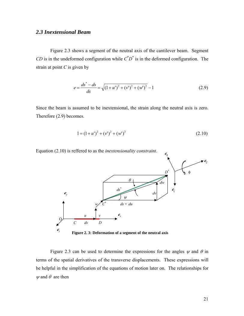
2.3 Inextensional Beam
Figure 2.3 shows a segment of the neutral axis of the cantilever beam. Segment
CD is in the undeformed configuration while C*D* is in the deformed configuration. The
strain at point C is given by
1)'()'()'1( 222*
−+++=−
= wvuds
dsdse (2.9)
Since the beam is assumed to be inextensional, the strain along the neutral axis is zero.
Therefore (2.9) becomes.
(2.10) 222 )'()'()'1(1 wvu +++=
Equation (2.10) is reffered to as the inextensionality constraint.
Figure 2. 3: Deformation of a segment of the neutral axis
O
θ
D*
ds*
dw
dvψ
C*
ds
w
vu
DC
xe
ye
ze
ds + du
ηe
ξe
ζe
φ
Figure 2.3 can be used to determine the expressions for the angles ψ and θ in
terms of the spatial derivatives of the transverse displacements. These expressions will
be helpful in the simplification of the equations of motion later on. The relationships for
ψ and θ are then
21

'1
'tanu
v+
=ψ , 22 )'()'1(
'tanvu
w++
−=θ (2.11)
Equation (2.11) indicates ψ and θ are dependent on the spatial derivatives of the
displacement components u, v, and w. Therefore there are only four independent
variables for this problem, namely u, v, w, and φ.
2.4 Strain-Curvature Relations
This section presents the derivation of the strain tensor components in terms of
the curvature components. Figure 2.4 shows the beam cross section at arclength s for
both the deformed and undeformed configurations.
Figure 2. 4: Initial and deformed positions of an arbitrary point P
O S
ζ P* C* η
C η
P
ζ
xe
ye
ze
ye
ze
ηe
ζe
ξe
22

An arbitrary point P in the undeformed beam cross section moves to point P* in the
deformed cross section. The position vectors for points P and P* are defined from Figure
2.4 as
zyxP sCPOCr eee ζη ++=+=r (2.12)
ζη ζη eeeee +++++=+= zyxPwvusPCOCr )(***
*
r (2.13)
The distance differentials for points P and P* are given by
zyxP dddsrd eee ζη ++=r (2.14)
ζζηηξ ζςηη eeeee dddddsrdP
++++=*
r (2.15)
with the first term in (2.15) given by
(2.16) **'')'1( DCdswdsvdsuds zyx =+++= eeeeξ
which is obtained directly from Figure 2.3. Equations (2.14) and (2.15) are used to obtain
(2.17) ...22)(2 2** TOHdsddsddsrdrdrdrd PPPP ++−−=⋅−⋅ ζηρηζρηρζρ ξξζη
rrrr
where H.O.T. stands for higher order terms.
The difference of the squared distance differentials is related to the Green's strain
tensor by (Mase, 1970)
[ ] [ ] [ ]TijPPPP dddsdddsrdrdrdrd ζηεζη ⋅⋅=⋅−⋅ 2**rrrr (2.18)
The components of the strain tensor in terms of the curvature are found by expanding the
right hand side of (2.18) and comparing it to the right hand side of (2.17).
23

ζη ηρζρε −=11 , ξζρεγ −== 1212 2 , ξηρεγ == 1313 2 , 0332322 === εεε (2.19)
2.5 Lagrangian of Motion
The Lagrangian of motion is defined as
(2.20) ∫=−=l
dsVT0
lL
where T is the kinetic energy, V the potential energy, l the length of the beam and l the
Lagrangian density.
The kinetic energy has two components, one due to translation and one due to
rotation. The kinetic energy due to translation is given by
∫ ++=l
tr dswvumT0
222 )(21
&&& (2.21)
The kinetic energy due to rotation is given by
∫=l
Trot dsJT
0
]][][[21
ζηξζηξ ωωωωωω (2.22)
where [J] is the distributed inertia matrix. Because the local coordinate system coincides
with the principal axes of the beam, the product moments of inertia are zero (Budynas,
1999). Therefore, the inertia matrix [J] is given by
24

(2.23) [ ]⎥⎥⎥
⎦
⎤
⎢⎢⎢
⎣
⎡=
ς
η
ξ
JJ
JJ
000000
with the elements along the diagonal defined by
, , (2.24) ∫∫ +=A
ddJ ζηζηρξ )( 22
∫∫=A
ddJ ζηρζη2
∫∫=A
ddJ ζηρηζ2
Substituting (2.24) into (2.22), and adding (2.21) to the resulting expression yields the
expression for the total kinetic energy of the system.
∫ +++++=l
dsJJJwvumT0
222222 ])([21
ζζηηξξ ωωω&&& (2.25)
The potential energy is equal to the strain energy of the beam, which is calculated
using the strain tensor components in (2.19). Therefore, the total strain energy is given
by
∫ ∫∫ ++=l
A
dsddU0
131312121111 })({21 ζηγσγσεσ (2.26)
For this derivation, a linear relationship between the stress and the strain is assumed.
Therefore, Hooke's law can be used to relate the stress to the strain.
1111 εσ E≈ , 1212 γσ G≈ , 1313 γσ G≈ (2.27)
Substituting the strain tensor components from the previous section into (2.26) and
(2.27), and noting that the cross section is symmetric about the η and ζ axes, the strain
energy is written as
25

∫ ++=l
dsDDDU0
222 )(21
ζζηηξξ ρρρ (2.28)
where Dξ, Dη, and Dζ are the torsional and flexural rigidities, respectively. The potential
energy is then
∫ ++=l
dsDDDV0
222 )(21
ζζηηξξ ρρρ (2.29)
Equations (2.25) and (2.29) are substituted into (2.20) to obtain the final
expression for the Lagrangian. The inextensionality constraint in (2.10) must be
maintained during the variational process. To enforce this constraint, equation (2.10) is
attached to the Lagrangian density by using a Lagrange multiplier λ(s,t). The Lagrangian
density is then
])'()'()'1(1[
21)(
21
)(21)(
21
222222
222222
wvuDDD
JJJwvum
−−+−+++−
+++++=
λρρρ
ωωω
ζζηηξξ
ζζηηξξ&&&l (2.30)
The Lagragian resulting from substituting (2.30) into (2.20) is an example of an
augmented functional. Variational problems dealing with finding the extremal of an
augmented functional are known as isoperimetric problems (Török, 2000).
2.6 Extended Hamilton's Principle
The cantilever beam is subjected to non conservative forces such as viscous
damping and the generalized forces Qα (α= u, v, w, and φ). Therefore, the extended
26

Hamilton's principle (Meirovitch, 2001) is used to derive the equations of motion. The
extended Hamilton's principle can be stated as follows
(2.31) 0)(2
1
=+= ∫t
tNCWI δδδ L
where δL is the virtual change in mechanical energy, and δWNC the virtual work due to
non conservative forces. The virtual work due to non conservative forces is given by
(2.32) ∫ +++=l
wvuNC dsQwQvQuQW0
**** )( δφδδδδ φ
where Q*α (α= u, v, w, and φ) stands for the generalized non conservative forces defined
as
(2.33) αααα &cQQ −=*
The variation of the Lagrangian is given by
(2.34) ∫=l
ds0
lL δδ
The Lagrangian density is a functional of 13 variables, namely u,v,w,φ, their time and
space derivatives, and the Lagrange multiplier λ. Therefore, the variation of the
Lagrangian density is given by
∑= ∂
∂=
13
1ii
i
xx
δδ ll (2.35)
Equation (2.11) in section 2.3 is used to obtain the variations of ψ and θ.
27

22 )'()'1(')'1('''
''
' vuvuuvv
vu
u ++++−
=∂∂
+∂∂
=δδδψδψδψ (2.36)
')'()'1()'()'1(
]''')'1[('''
''
''
2222
wvuvu
vvuuwww
vv
uu
δδδδθδθδθδθ ++−++
++=
∂∂
+∂∂
+∂∂
= (2.37)
The preceding two equations are used to compute the variation of the Lagrangian density
given by (2.35). Taking the variation of the Lagrangian density and integrating by parts
several times results in
0}'
'''
)()(
)()({
0
0
*
0
*
0
*
0
*
'
''2
1
=⎥⎦
⎤⎢⎣
⎡∂∂
++++−−−
+−+++−
+++−+++−
=
∫∫
∫∫ ∫
dtwHvHuHwGvGuG
dsAQwdsGQwm
vdsGQvmudsGQum
l
swvuwvu
ll
ww
l
vv
t
t
l
uu
δφφ
δδδδδδ
δφδ
δδ
φφ
l
&&
&&&&
(2.38)
with Gu, Gv, and Gw given by
)'1(''
uu
Au
AGu ++∂∂
+∂∂
= λθψθψ , '
''v
vA
vAGv λθψ
θψ +∂∂
+∂∂
= , ''
ww
AGw λθθ +
∂∂
= (2.39)
and Aψ, Aθ, Aφ, Hu, Hv, and Hw given by
),,(
''''
),,('
22
wvuH
stA
=∂∂
∂∂
+∂∂
∂∂
=
=∂∂
−∂∂
∂+
∂∂∂
=
ααθ
θαψ
ψ
φθψαααα
α
α
ll
lll& (2.40)
Equation (2.38) is valid for any arbitrary δu, δv, δw and δφ, implying that the
individual integrands be equal to zero (Török, 2000). Thus the equations and boundary
conditions for the flexural-flexural-torsional vibrations of a cantilever beam are given by
28

uu GQum '* =−&& , , , vv GQvm '* =−&& ww GQwm '* =−&& φφ AQ =*
0'
'''0
=⎥⎦
⎤⎢⎣
⎡∂∂
++++−−−=
l
swvuwvu wHvHuHwGvGuG δφ
φδδδδδδ l (2.41)
2.7 Order Three Equations of Motion
The equations of motion derived in the previous section are simplified to include
nonlinear effects up to order three. This is accomplished by expanding each term in the
equations into a Taylor series and discarding terms of order greater than three. The
simplification is necessary to enable the use of the equations to study the motion of the
beam via numerical techniques. Previous mathematical models for the non linear
vibration of cantilever beams included nonlinearities up to order two (Crespo da Silva,
1978). This model is more complete since it incorporates nonlinearities up to order three.
The simplification process begins by obtaining the order three Taylor series
expansions of u', ψ, and θ. These are derived using the Taylor series expansion of
arctan(x)
...31tan 31 +−=− xxx (2.42)
which is combined with (2.10), and (2.11) to get
...])'()'[(211])'()'(1[' 222122 ++−=−−−= wvwvu (2.43)
...])'(21)'(
611['}])'()'(1['{tan
'1'tan 22212211 +++=−−=
+= −−− wvvwvv
uvψ (2.44)
...])'(611['}])'(1['{tan
])'()'1[('tan 22/121
2/1221 ++−=−−=
++−
= −−− wwwwvu
wθ (2.45)
29

The order three expansion for the angle of twist is obtained from the twisting
curvature ρξ. The third order expansion for the twisting curvature is given by
'"' wv+= φρξ (2.46)
Equation (2.46) is integrated over the length of the beam to obtain the order three
expression for the angle of twist.
(2.47) ∫+≡s
dswv0
'"φγ
Expanding the remaining terms in (2.41) and retaining terms up to order three
yields
'''
)}'1(''''''''
])''(')''(')[()''''''('{
uwwDvvD
wvvwDDwvvwDQucum uu
++++
+−−−=−+
λ
γγγ
ηζ
ζηξ&&& (2.48)
'
'''
}')])''()''((''''[
'''''')''()'')[(('''{
220
2
vwvvvD
dswvwvwDDwDQvcvms
vv
λ
γγγ
ζ
ζηξ
+++−
+−−+−=−+ ∫&&& (2.49)
'
'''
}')])''()''((''''[
]'''''')''()'')[((''{
220
2
wwvwwD
dsvwvwvDDvDQwcwms
ww
λ
γγγ
η
ζηξ
+++−
−+−+=−+ ∫&&& (2.50)
]''''))''()''(()[('' 22 wvwvDDD −−−= γγ ζηξ (2.51)
which are the order three equations of motion for the cantilever beam.
The boundary conditions for the fixed end are given by
)',',,,,(0),0( wvwvut γαα == (2.52)
30

The natural boundary conditions obtained from (2.41-e) are used for the free end of the
beam. Thus, the boundary conditions for the free end are given by
)','1
','1
'(0),( γααu
wHHu
vHHtl uwuv +−
+−== (2.53)
),,(0),( wvutlG == αα (2.54)
Equations (2.49) and (2.50) are further simplified by removing λ and γ using the
Taylor series expansions of u, λ and γ. The expansion of u is obtained directly from
(2.43) as
∫ +−=s
dswvu0
22 ])'()'[(21 (2.55)
Equations (2.55), (2.47), (2.48), (2.49), and (2.50) suggest u, λ and γ are of order two.
Equation (2.55) is substituted into (2.48) and only terms up to order two are kept.
Integrating the resulting expression from l to s, produces the expression for the Lagrange
multiplier λ in terms of the transverse displacements. Incidentally, the Lagrange
multiplier is interpreted as an axial force necessary to maintain the inextensionality
constraint (Malatkar, 2003).
∫∫ ∫ −+∂∂
−−−=s
lu
s
l
s
dsQdsdswvt
mwwDvvD ]])'()'[([21''''''''
0
222
2
ηζλ (2.56)
For the angle of twist, (2.51) is integrated twice and only terms up to order two
are retained. The angle of twist is then
∫ ∫−
−=s s
l
dsdswvD
DD
0
''''ξ
ζηγ (2.57)
31

Equation (2.57) indicates flexure induced torsion is a nonlinear phenomenon (Malatkar,
2003).
Substituting (2.56) and (2.57) into (2.49) and (2.50) yields the order three
equations of motion for the flexural-flexural-torsional vibration of a cantilever beam.
∫∫ ∫
∫ ∫
∫∫
−+∂∂
−
+−−
−
⎥⎦
⎤⎢⎣
⎡−−+=++
s
lu
s
l
s
s s
l
ss
lv
ivv
dsQvdsdswvt
vm
wwvvvDdsdswvwD
DD
dswvwdswvwDDQvDvcvm
''
''''
)'(}])''(['{21
})''''''('{})''''''()(
'"'''""''){(
0
222
2
0
2
0
ζξ
ζη
ζηζ&&&
(2.58)
∫∫ ∫
∫ ∫
∫∫
−+∂∂
−
+−−
+
⎥⎦
⎤⎢⎣
⎡−−−=++
s
lu
s
l
s
s s
l
ss
lw
ivw
dsQwdsdswvt
wm
wwvvwDdsdswvvD
DD
dsvwvdswvvDDQwDwcwm
''
''''
)'(}])''(['{21
})''''''('{})''''''()(
'"'''""''){(
0
222
2
0
2
0
ηξ
ζη
ζηη&&&
(2.59)
The boundary conditions for (2.58) and (2.59) are given by
0),(''',0),(''',0),(",0),("0),0(',0),0(',0),0(,0),0(
========
tlwtlvtlwtlvtwtvtwtv
(2.60)
The boundary conditions for the free end are derived from (2.53).
The equation of motion and boundary conditions for the forced planar flexural
vibration of the beam is obtained from equations (2.58) and (2.59). For planar motion,
equation (2.59) is dropped along with the w terms in (2.58). With these substitutions
equation (2.58) becomes
32

∫∫ ∫ −∂∂
−−=++s
lu
s
l
s
viv
v dsQvdsdsvt
vmvvvDQvDvcvm '''' )'(}]'['{21})'''('{
0
22
2
ζζ&&& (2.61)
For base excitation of the vertical beam, the transverse displacement v is given by
)cos(0 tvvv b Ω+= (2.62)
where vb is the transverse displacement of the beam relative to the base, v0 the amplitude
of the excitation at the base, and Ω the excitation frequency. Moreover, the generalized
force Qv is zero and the generalized force Qu is the weight per unit length.
0, == vu QmgQ (2.63)
Substituting (2.62) and (2.63) into (2.61) yields the equation for the planar
flexural forced vibration of the beam
tAadsdsv
tvA
vvvEIvlsvAgEIvvcvA
b
s
l
s
ivv
Ω+∂∂
−
−+−=++
∫ ∫ cos}]'['{21
})'''('{]')(''[
'
''
0
22
2
ρρ
ρρ &&&
(2.64)
where ρ, A, cv, E, I, and ab are the density, cross sectional area, viscous damping
coefficient, Young's modulus, moment of inertia and acceleration applied at the base,
respectively.
The first term on the right hand side of (2.64) arises from the effect of gravity on
the beam. The second and third terms represent the curvature and inertia nonlinearity,
respectively.
33

Chapter 3: Numerical Solution
This chapter develops the numerical algorithm used to solve the equation of
motion for the planar flexural forced vibration of the cantilever beam (2.64). The partial
differential equation is first discretized in the spatial coordinate using Galerkin's weighted
residual method (Section 3.1). Then, the equation is discretized in the time domain using
the Newmark technique (Section 3.2). Finally, a numerical algorithm is used to calculate
the nonlinear response of the beam (Section 3.3).
3.1 Finite Element Model
The equation of motion for the nonlinear planar flexural forced vibration of a
cantilever beam was derived in the previous chapter. The equation of motion for the
transverse displacement in the y direction is given by
tAadsdsv
tvA
vvvEIvlsvAgEIvvcvA
b
s
l
s
ivv
Ω+∂∂
−
−+−=++
∫ ∫ cos}]'['{21
})'''('{]')(''[
'
''
0
22
2
ρρ
ρρ &&&
(3.1)
This equation can be written in the form
0}'{21}'{ '' 213 =−++−++ FfvAfvEIAgfEIvvcvA iv
v ρρρ &&& (3.2)
with the functions f1, f2, f3 , and F given by
, ')'''(1 vvf = ∫ ∫∂∂
=s
l
s
dsdsvt
f0
22
2
2 ' , '")(3 vvlsf +−= , tAaF b Ω= cosρ (3.3)
34
The functions f1, f2, and f3 originate from the curvature, inertial, and gravitational
nonlinear effects, respectively. The function F is the force associated with the transverse
displacement exciting the base of the beam.
Equation (3.2) is a nonlinear integro-differential equation, for which a closed
form solution is not available. Therefore, an approximate solution is sought by
discretizing (3.2), first in the spatial coordinate using Galerkin's weighted residuals
method, and then in the time domain using the Newmark technique.
The discretization in the spatial coordinate is carried out in three steps: (1) mesh
generation and function approximation, (2) element equation, and (3) assembly and
implementation of boundary conditions. These steps are discussed in detail in the
remaining of this section. The discretization in the time domain is the focus of section
3.2.
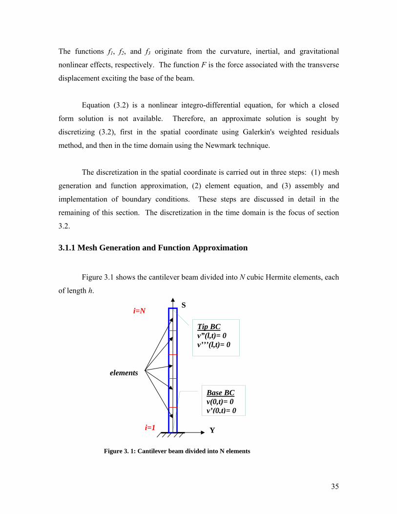
3.1.1 Mesh Generation and Function Approximation
Figure 3.1 shows the cantilever beam divided into N cubic Hermite elements, each
of length h.
S
Figure 3. 1: Cantilever beam divided into N elements
i=N
i=1
elements
Y
Tip BC v”(l,t)= 0 v’’’(l,t)= 0
Base BC v(0,t)= 0 v’(0,t)= 0
35

h
qj+1 , q'j+1 qj , q'j j y
s
j+1
Figure 3. 2: Typical cubic Hermite beam element
The typical cubic Hermite element (Figure 3.2) has two nodes with two degrees of
freedom per node (Zienkiewicz, 1977), namely translation (qj) and slope (q'j ). The
displacement of any point inside the element is approximated as
(3.4) )()(),(~ 4
1tqstsv
j
ejj
e ∑=
= ψ
The shape functions ψj(s) are given by (Reddy, 1993).
32
1 231 ⎟⎠⎞
⎜⎝⎛+⎟
⎠⎞
⎜⎝⎛−=
hs
hsψ ,
⎥⎥⎦
⎤
⎢⎢⎣
⎡⎟⎠⎞
⎜⎝⎛+⎟
⎠⎞
⎜⎝⎛−⎟
⎠⎞
⎜⎝⎛=
32
2 2hs
hs
hshψ ,
32
3 23 ⎟⎠⎞
⎜⎝⎛−⎟
⎠⎞
⎜⎝⎛=
hs
hsψ ,
⎥⎥⎦
⎤
⎢⎢⎣
⎡⎟⎠⎞
⎜⎝⎛+⎟
⎠⎞
⎜⎝⎛−=
32
4 hs
hshψ (3.5)
The vector in (3.4) is the element nodal displacement vector. For the remaining of
this derivation, the superscript e is dropped for the sake of simplicity. The numerical
solution of the partial differential equation in (3.2) is a piecewise cubic polynomial
comprised of the sum of the approximated displacement
ejq
),(~ tsv e , i.e., ∑≅e
evv ~ .
36

3.1.2 Element Equation
In order to obtain the element equation, the approximated displacement in (3.4) is
substituted into the partial differential equation (3.2). When this is done, the left hand
side is no longer equal to zero, but to a quantity Rx called the residual.
xj
jjj
jj
jj
ivj
jjjv
jjj
RfqAfqEI
AgfFqEIqcqA
=++
−−++
∑∑
∑∑∑
==
===
'' ])'[(21])'[( 2
4
11
4
1
3
4
1
4
1
4
1
ψρψ
ρψψψρ &&&
(3.6)
The weighted residual WR is defined using Galerkin's method. In Galerkin's
method, the shape function ψi is used as the weighting function. The weighted residual
is forced to be zero over the element. Therefore WR is given by
(3.7) ∫ ==h
xi dsRWR0
0ψ
Multiplying both sides of (3.6) by the shape function ψi and integrating over the length of
the element results in
0])'[(21])'[(
][][][
'' 20
4
11
0
4
13
0
0
4
1 0
4
1 0
4
1 0
=++−
−++
∫ ∑∫ ∑∫
∫∑∫∑∫∑∫
==
===
dsfqAdsfqEIdsfAg
FdsqdsEIqdscqdsA
j
h
jjij
h
jji
h
i
h
ij
j
hiv
jij
j
h
jivj
j
h
ji
ψψρψψψρ
ψψψψψψψρ &&&
(3.8)
Finally, several terms in equation (3.8) are integrated by parts to obtain the weak
form of the element equation
37

0]"''''[]'[]'[
]''21[]''[
]""[][][
00201
021
003
0000
=−+++
−−−
−++
∑∑∑∑
∑∫∑∫∫
∫∑∫∑∫∑∫
hj
jji
jjji
h
jjji
h
jjji
jj
h
jijjj
h
i
h
i
h
ijj
h
jijj
h
jivj
h
jji
qEIqEIfqEIfq
qdsfAqdsfEIdsfAg
FdsqdsEIqdscqdsA
ψψψψψψψψ
ψψρψψψρ
ψψψψψψψρ &&&
(3.9)
which can be simplified to
(3.10) 0=+−−−−++ ei
ei
eij
eijj
eijj
eijj
eijj
eij bgFqkiqkcqKqcqM &&&
with the matrices, , , and given by eijM e
ijc eijK
(3.11) ∫∫∫ ===h
jieij
h
jiveij
h
jieij dsEIKdsccdsAM
000
"",, ψψψψψψρ
These matrices are the element mass, damping and stiffness matrices, respectively.
Equation (3.10) is written in indicial notation. Therefore, repeated indices denote
summation.
At this point it is convenient to introduce the matrix naming convention used in
the remaining of the chapter. Matrices in capital letters are linear matrices, while
matrices in lower case letters are nonlinear matrices. For instance, in (3.11) the matrices
and, are linear matrices, while the matrix is a nonlinear matrix. eijM e
ijK eijc
For a cubic Hermite beam element the matrices and, are given by
(Reddy, 1993)
eijM e
ijK
38

⎥⎥⎥⎥
⎦
⎤
⎢⎢⎢⎢
⎣
⎡
−−−−−−
=
22
22
422313221561354313422135422156
420hhhh
hhhhhhhh
AhM eij
ρ (3.12)
⎥⎥⎥⎥
⎦
⎤
⎢⎢⎢⎢
⎣
⎡
−−−−
−−
=
22
22
3
4626612612
2646612612
hhhhhhh
hhhhhh
hEIK e
ij (3.13)
where ρ, A, E, I, and h are the density, cross sectional area, Young’s modulus, area
moment of inertia and length of the element, respectively.
Equation (3.10) has two additional stiffness matrices eijkc d e
ijki , resulting from
the nonlinear effects in (3.2). These matrices are given by
, an
, ∫=h
jieij dsfEIkc
01'' ψψ ∫=
h
jieij dsfAki
02''
21 ψψρ (3.14)
The matrix represents the curvature nonlinearity, while represents the inertia
nonlinearity.
eijkc e
ijki
The vectors e and are the force and gravitational effect vectors, respectively
and are defined as
iF eig
, (3.15) ∫=h
ie
i FdsF0
ψ ∫=h
iei dsfAgg
03ψρ
The vector is the combination of the boundary terms in (3.9). eib
(3.16) hii
hi
hi
ei vvv'vb 000 ]'[]'[)]"('[ MVFMV a ψψψψ −+++=
39

The quantities V and M in (3.16) are the transverse shear force and bending moment of
the beam. For a beam, the bending moment and shear force are given by (Rao, 1990)
"EIv=M , ')"(EIv=V (3.17)
The force Fa in (3.16) can be interpreted as part of the axial force required to
maintain the inextensionality constraint. The origin of Fa is understood upon
examination of the order two expression for the Lagrange multiplier derived in the
previous chapter.
The Lagrange multiplier is interpreted as the axial force required to maintain the
inextensionality constraint (Malatkar, 2003). Recall from Chapter 2, the order two
expression for the Lagrange multiplier is
∫∫ ∫ −+∂∂
−−−=s
lu
s
l
s
dsQdsdswvt
mwwDvvD ]])'()'[([21''''''''
0
222
2
ηζλ (3.18)
For planar motion of the cantilever beam (3.18) becomes
)(]'[21''''
0
22
2
lsAgdsdsvt
AvEIvs
l
s
−−∂∂
−−= ∫ ∫ ρρλ (3.19)
which can be written as
bae WFF −−−=λ (3.20)
with Fe, Fa, and Wb given by
' , ''' vEIv=eF dsdsvt
As
l
s
∫ ∫∂∂
= ]'[21
0
22
2
ρaF , )( lsAg −= ρbW (3.21)
40

From (3.20) it is clear the Lagrange multiplier λ is the combination of three
forces, namely the elastic force (Fe), the inertial force (Fa) and the weight of the beam
above point s along the neutral axis (Wb). Hence, Fa is indeed part of the axial force
required to maintain the inextensionality constraint.
3.1.3 Assembly and Implementation of Boundary Conditions
Assembly of the N element equations yields the global finite element equation
iijijjijjij bfqkqcqM +=++ &&& (3.22)
which is a system of 2(N+1) ordinary differential equations, i.e., one for each nodal
degree of freedom. The solution of this system is the vector , which contains the nodal
displacements and nodal rotations in the global coordinates S and Y (Figure 3.1). The
global linear mass matrix is calculated using (3.12).
jq
ijM
The nonlinear damping matrix is calculated using proportional damping
(Cook, 1995). Therefore, is approximated as a linear combination of the mass and
nonlinear stiffness matrices.
ijc
ijc
ijijij kMc 21 αα += (3.23)
The coefficients α1 and α2 are calculated using the natural frequencies and modal
damping ratios of the system. The procedure to calculate these coefficients is discussed
in detail in section 3.3.
41

The nonlinear stiffness matrix is the combination of the linear stiffness matrix,
calculated using (3.13), and the two nonlinear stiffness matrices and , calculated
with (3.14).
ijk
ijkc ijki
ijijijij kikcKk −−= (3.24)
The nonlinear force vector is the combination of the linear force vector and the
gravitational effect vector, both calculated with (3.15).
if
iii gFf += (3.25)
The boundary vector is defined using the element boundary vector given by
(3.16). The internal reactions V, M, and Fa in (3.16) cancel out upon assembly for all
nodes except for the first and last nodes. Therefore, the global boundary vector has non
zero elements only at the fixed and free ends of the beam. The boundary conditions of the
problem are used to evaluate bi. From the previous chapter the boundary conditions are
ib
0),(''',0),("
0),0(',0),0(==
==tlvtlv
tvtv (3.26)
The elements of the boundary vector for the fixed end are given by
MVFMV
MVFMV
a
a
'')"(''')"('
22222
11111
ψψψψψψψψ−+++=
−+++=vvv'vb
vvv'vb (3.27)
For the fixed end, v' is zero according to the boundary conditions in (3.26). Therefore, the
first two terms of b1 and b2 vanish and (3.27) becomes
MV '111 ψψ −=b , MV '222 ψψ −=b (3.28)
42

The elements of the boundary vector corresponding to the free end are
a
a
FVMMV
FVMMV
'')"('
'')"('
4444)1(2
33331)1(2
vvv'vb
vvv'vb
N
N
ψψψψ
ψψψψ
++−+=
++−+=
+
−+ (3.29)
For the free end, both v" and v''' are zero from the boundary conditions. As a result, both
the shear force and bending moment are zero according to (3.17), causing the first three
terms in (3.29) to vanish. Also, the inertial force Fa is zero at the free end, according to
(3.21). Therefore, both and are zero. 1)1(2 −+Nb )1(2 +Nb
0)1(21)1(2 == +−+ NN bb (3.30)
Since the displacement and rotation at the fixed end are both known from the
boundary conditions, the first two equations in (3.22) do not need to be included as part
of the system of equations to be solved. These equations are saved for post processing of
the solution.
Substituting the boundary vector into (3.22), and saving the first two
equations of the system for post processing yields
ib
(3.31) rij
rijj
rijj
rij fqkqcqM =++ &&&
The superscript r in (3.31) stands for reduced, since the first two equations are
eliminated.
3.2 Newmark Technique
In this section, the linear global finite element equation of motion is used to
illustrate the Newmark technique. The linear equation of motion is given by
43

(3.32) ijijjijjij FQKQCQM =++ &&&
djQ
Figure 3. 3: Interval for discretization in the time domain
and is obtained by omitting the nonlinear matrices and , as well as the
gravitational effect vector in (3.31). The matrices , , and the vector are
reduced matrices since the first two rows and columns are eliminated. However, the
superscript r is dropped for simplicity.
ijkc ijki
ig ijM ijC ijK iF
Equation (3.32) is discretized within the time interval [-Δt,Δt], where Δt is the
time step (Figure 3.3) and t is an arbitrary time. This interval is divided in two segments
of length Δt each. Dividing the interval in this manner creates three discrete time points
(Figure 3). For each one of these time nodes5 there is a displacement vector associated to
it. The displacement vector for time Δt is , while the displacement vectors for times
0 and -Δt are and , respectively.
1+djQ
djQ 1−d
jQ
The displacement vector at any time inside the interval in Figure 3.3 is
approximated by6
(3.33) kjk
djd
djd
djdj QQQQQ Φ=Φ+Φ+Φ= +
+−
−1
11
1
where Φd-1, Φd, and Φd+1 are the shape functions given by (Zienkiewicz, 1977)
5 Nodes in the time interval are called time nodes from now on, to avoid confusion with the nodes used for the discretization in the spatial coordinate (section 3.1). 6 Equation (3.33) is written in indicial notation. Therefore, repeated indices denote summation.
2Δt
t = -Δt t = Δt Δt Δt
1+djQ1−d
jQ
t = 0
44

)1(21 νν
−−
=Φ −d , )1)(1( νν +−=Φd , )1(21 νν
+=Φ +d (3.34)
The dimensionless time coordinate ν in (3.34) is defined as
t
tΔ
=ν (3.35)
The displacement vector in (3.33) is a quadratic polynomial in t. The force inside the
interval [-Δt, Δt] is interpolated in a way similar to the displacement vector (Zienkiewicz,
1977). Therefore the force Fi is given by
jQ
(3.36) kik
did
did
didi FFFFF Φ=Φ+Φ+Φ= +
+−
−1
11
1
Substitution of (3.33) and (3.36) into (3.32) yields the residual Rt.
(3.37) tk
ikkjkij
kjkij
kjkij RFQKQCQM =Φ−Φ+Φ+Φ &&&
with k ranging from d-1 to d+1. The weighted residual method is applied by multiplying
(3.37) by a weighting function ω(t) and integrating from -Δt to Δt. Equation (3.37)
becomes then
(3.38) ∫Δ
Δ−
=Φ−Φ+Φ+Φt
t
kik
kjkij
kjkij
kjkij dtFQKQCQMt 0])[( &&&ω
Substituting the shape functions (3.34) into (3.38) results in
(3.39)
0})5.0()25.0({
})5.0()1({})25.0(
)21(2{}{
112
122
12
=−+++−+Δ−
Δ−++Δ−−+Δ+−+
Δ−+−+Δ+Δ+
−+
−
+
di
di
di
djijijij
djij
ijijdjijijij
FFFt
QKttCMQKt
tCMQKttCM
γβγββ
γβγγβ
γβγ
45

where the quantities γ and β are given by
∫
∫
−
−
+= 1
1
1
1
)(
)21)((
ννω
νννωγ
d
d,
∫
∫
−
−
+= 1
1
1
1
)(
)1)((21
ννω
ννννωβ
d
d (3.40)
Notice the variable of integration in (3.40) has been changed from t to the dimensionless
time coordinate ν (3.35).
Equation (3.39) can be simplified to
(3.41) 0321 11 =−++ −+i
djij
djij
djij QAQAQA F
where the matrices and the vector are defined as follows ijA1 , ijA2 , ijA3 iF
(3.42)
ijijijij
ijijijij
ijijijij
KttCMA
KttCMA
KttCMA
2
2
2
)5.0()1(3
)25.0()21(22
1
Δ−++Δ−−=
Δ+−+Δ−+−=
Δ+Δ+=
γβγ
γβγ
βγ
(3.43) })5.0()25.0({ 112 −+ −+++−+Δ= di
di
dii FFFt γβγββF
Equation (3.41) is used to solve for the displacement vector in terms of the
displacement vectors and .
1+djQ
djQ 1−d
jQ
(3.44) iijdlilij
dlilij
dj AtQAAQAAQ F1211`11 13121 −−−−+ Δ+−=
46

Figure 3. 4: Time nodes in [0,TF]
The use of (3.44) to calculate the time history of the displacement vector in
the interval [0,TF] is illustrated next. Here TF is an arbitrary time. The time interval
[0,TF] has TN time nodes with TN given by (Figure 3.4)
jQ
1+Δ
=t
TFTN (3.45)
The first time node corresponds to d=1, the second to d=2, and so on.
The displacement vector for the second time node in [0,TF] is simply . In order
to calculate , the vectors and must be prescribed. This is done by using the
initial conditions of the problem. For this problem it is assumed the beam starts from
rest, which means the displacement vectors and are equal to the zero vector.
1jQ
1jQ 0
jQ 1−jQ
0jQ 1−
jQ
(3.46) 010 == −jj QQ
Substituting d=0 along with (3.46) into (3.44) yields
iijj AtQ F121 1−Δ=
(3.47)
s manner (3.44) is
sed to calculate the displacement vectors for all time nodes in [0,TF].
The force vector iF is given by (3.43). The vectors jQ and jQ are substituted in (3.44)
to calculate 2jQ , the displacement vector for the next time node. In thi
0 1
u
Δt
... t= 2Δt t= Δt
0jQ
t= TF
1jQ 2
jQ 1−TNjQ
t= 0
47
The quantities γ and β in (3.40) vary depending on the choice for weighting
function ω(ν). For this problem, the values γ = 0.5 and β = 0.25 are used. This
corresponds to an average acceleration scheme (Zienkiewicz, 1977). These values of γ
and β ensure the computation of the time history of the displacement vector using (3.44)
unconditionally stable, i.e., independent of the size of Δt (Bathe, 1973).
.3 Numerical Algorithm
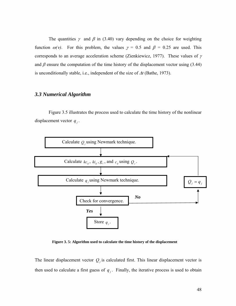
st es the process used to calculate the time history of the nonlinear
isplacement vector .
Figure 3. 5: Algorithm used to calculate the time history of the displacement
al
then used to calculate a first gu f . Finally, the iterative process is used to obtain
is
3
Figure 3.5 illu rat
jqd
Yes
No
Calculate ijkc , ijki , ig , and ijc using jQ .
Calculate jQ using Newmark technique.
Calculate jq using Newmark technique.
Check for convergence.
Store jq .
jj qQ =
The linear displacement vector jQ is c culated first. This linear displacement vector is
ess o jq
48

the nonlinear displacement vector for time t. This algorithm is implemented in the
Matlab® program NLB
jq7 in Appendix A.
3.3.1 Calculation of the Linear Displacement Qj
The Newmark technique is used to calculate the linear displacement vector Qj in
the interval [0,TF], with 0 < t < TF. This interval is divided in TN time nodes with TN
defined by (3.45).
t - 2Δt t
djQ
Δt Δt 1+d
jQ1−djQ
t - Δt
Figure 3. 6: Displacement vectors used to calculate Qj at time t
The linear displacement vector at time t is given by
(3.48) iijdlilij
dlilij
dj AtQAAQAAQ F1211`11 13121 −−−−+ Δ+−=
where , are the linear displacement vectors for times t - Δt, and t - 2Δt,
respectively (Figure 3.6).
djQ 1−d
jQ
The matrices , , and are calculated using the global linear mass and
stiffness matrices.
ijA1 ijA2 ijA3
7 Non Linear Beam
49

(3.49)
ijijijij
ijijijij
ijijijij
KttCMA
KttCMA
KttCMA
2
2
2
)5.0()1(3
)25.0()21(22
1
Δ−++Δ−−=
Δ+−+Δ−+−=
Δ+Δ+=
γβγ
γβγ
βγ
The coefficients γ and β are taken as 0.5 and 0.25, respectively. This corresponds to the
average acceleration scheme (Zienkiewicz, 1977).
The matrix is the linear damping matrix and is calculated as a linear
combination of the mass and stiffness matrices (Cook, 1995). Thus is given by
ijC
ijC
ijijij KMC 21 αα += (3.50)
The coefficients α1 and α2 are obtained by solving the system
22
,22
42
4
14
12
1
11
ωαωα
ξωα
ωα
ξ +=+= (3.51)
The focus of this investigation is the time response of the cantilever beam when the base
is excited at a frequency close to the third natural frequency. Therefore, the first and
fourth natural frequencies and modal damping ratios are used in (3.51).
The force vector in (3.48) is calculated as
(3.52) })5.0()25.0({ 112 −+ −+++−+Δ= di
di
dii FFFt γβγββF
where , , and are the linear force vectors for times t, t - Δt, and t - 2Δt,
respectively (Figure 3.6).
1+diF d
iF 1−diF
50

3.3.1 Calculation of the Nonlinear Displacement qj
The nonlinear displacement vector at an arbitrary time t in [0,TF] is given by
(3.53) iijdlilij
dlilij
dj atqaaqaaq f1211`11 13121 −−−−+ Δ+−=
where , are the nonlinear displacement vectors for times t - Δt, and t - 2Δt,
respectively (Figure 3.8).
djq 1−d
jq
t - 2Δt t
djq
Δt Δt 1+d
jq
t - Δt
1−djq
Figure 3. 7: Displacement vectors used to calculate qj at time t
The matrices , and in (3.53) are calculated using the global linear
mass matrix and the nonlinear stiffness matrix given by (3.24).
ija1 ija2 ija3
ijk
(3.54)
ijijijij
ijijijij
ijijijij
kttcMa
kttcMa
kttcMa
2
2
2
)5.0()1(3
)25.0()21(22
1
Δ−++Δ−−=
Δ+−+Δ−+−=
Δ+Δ+=
γβγ
γβγ
βγ
The coefficients γ and β are taken as 0.5 and 0.25, respectively. This corresponds to the
average acceleration scheme (Zienkiewicz, 1977).
In order to obtain the nonlinear stiffness matrix , the functions f1 and f2 defined
in (3.3-a) and (3.3-b) must be calculated. These functions are used with (3.14) to
compute the nonlinear stiffness matrices and , which are substituted into (3.24) to
ijk
ijkc ijki
51

obtain . A detailed example of the procedure used to calculate is included in
Appendix D. The matrix is calculated using a similar procedure.
ijk ijki
ijkc
The matrix is the nonlinear damping matrix and is calculated as a linear
combination of the mass and stiffness matrices (Cook, 1995).
ijc
ijijij kMc 21 αα += (3.55)
The coeffiecients α1 and α2 are the same as in section 3.3.1.
The force vector in (3.53) is calculated as
(3.56) })5.0()25.0({ 112 −+ −+++−+Δ= di
di
dii ffft γβγββf
where , , and are the nonlinear force vectors for times t, t - Δt, and t - 2Δt,
respectively (Figure 3.7).
1+dif d
if 1−dif
The nonlinear force vector is simply the combination of the linear force vector
and the gravitational effect vector (3.25). The gravitational effect vector is calculated
using a procedure similar to the one illustrated in Appendix D.
if
3.3.3 Iterative Procedure
The iterative procedure used to obtain the nonlinear displacement vector at any
given time t is illustrated in Figure 3.5. Once vectors and are obtained as
discussed in sections 3.3.1 and 3.3.2, the error θ is calculated
jQ jq
52

mj
mj
k
mQq −= ∑
=1θ
TOL≤θ for convergence (3.57)
where k is the total number of elements in each vector.
The error θ is compared to a maximum allowed error TOL. Once TOL≤θ , the
solution is converged and the vector is stored. However, if the error θ exceeds the
maximum allowed error, is assigned to and a new is calculated (Figure 3.5).
This procedure is repeated until convergence is achieved.
jq
jq jQ jq
53

Chapter 4: Time Response
This chapter is devoted to the study of the time response of the cantilever beam.
The experimental results, obtained by Malatkar (2003), for the steady state response of
the beam are presented first. These experimental results are compared with the
corresponding numerical results, obtained with the NLB8 program in Appendix A. Then
the NLB program is used to calculate the transient response of the beam, which is
compared against results from a finite element model developed in ANSYS®.
4.1 Experimental Steady State Response
Figure 4.1 shows the experimental set up used by Malatkar (2003) to measure the
time response of the cantilever beam when subjected to harmonic excitation at the base.
The beam is made of steel with Young's modulus of 165.5 GPa, density of 7400 kg/m3
and dimensions as indicated in Figure 4.1.
x
Figure 4. 1: Experimental set up
8 Non Linear Beam
strain gage
35 mm
0.55 mm
12.71 mm
662 mm
shaker
beam
excitation
accelerometer Beam cross section
y
54

The shaker excites the base of the beam in the y direction (Figure 4.1). An
accelerometer is attached at the same point to monitor the input excitation to the beam. A
strain gage is mounted approximately 35 mm from the base. At this location the strains
are maximum and also easy to measure. The strain read at the base is used to obtain the
frequency response.
The harmonic excitation applied by the shaker to the base of the beam is given by
tAaF b Ω= cosρ (4.1)
where ρ, A, ab, and Ω are the density, cross sectional area, maximum amplitude of
acceleration at the base, and excitation frequency, respectively. Malatkar (2003) used an
excitation frequency of 17.547 Hz with a maximum amplitude of acceleration equal to
2.97g, where g is the acceleration due to gravity. Transients were allowed to die out
before the response was recorded.
Figure 4. 2: Time response for Ω= 17.547 Hz, ab= 2.97g
Figure 4. 3: FFT for Ω= 17.547 Hz, ab= 2.97g
55

Figure 4.2 shows the time response of the vertical cantilever beam (Figure 4.1)
when Ω= 17.547 Hz and ab= 2.97g. This excitation frequency is close to the third
natural frequency of the beam (Table 4.1). The time response of the beam consists of a
high frequency component modulated by a low frequency component.
Table 4. 1: Experimental natural frequencies and damping ratios9
Mode number (n) fn(Hz) ξn
1 0.574 0.009
2 5.727 0.00185
3 16.55 0.00225
4 32.67 0.005
The response in Figure 4.2 is not the actual displacement, but the strain reading
in Volts. However, the frequency response obtained with the strain reading will be the
same as the frequency response obtained using the actual displacement. Hence, the strain
results can be used to determine the frequency response of the beam at the base.
The FFT shown in Figure 4.3 is used to determine the actual frequency
components present in the time trace (Figure 4.2). The high frequency component is
centered at 17.547 Hz, i.e., the excitation frequency. The asymmetric sideband structure
around the high frequency peak indicates the third mode frequency component is
modulated (Malatkar, 2003). The modulation frequency can be calculated from the
sideband spacing, and it is found to be 1.58 Hz for this case.
Figure 4.3 also indicates the presence of a low frequency component in the
response. This low frequency component is centered at 1.58 Hz, i.e., the modulation
frequency of the high frequency component. Anderson, et al. (1992) found the low
frequency component in the response of a beam excited close to a high frequency mode,
is equal to the modulation frequency of the high frequency component. 9 Natural frequencies measured by Malatkar (2003) for the vertical beam. The natural frequencies are lower than for a horizontal beam (Table B.1) due to the effect of gravity (Blevins, 1979).
56

4.2 Numerical Steady State Response
The numerical results for the response of a point at the base of the beam are
presented next. The results were obtained with the program NLB, included in Appendix
A. The beam dimensions and material properties used are the same as in section 4.1 The
cantilever beam was meshed with 20 elements. Thus, the length of each element is
33.1 mm. Moreover, each element was divided into 10 subdivisions, resulting in a Δx of
3.1mm (see Appendix D, Figure D.1). A time step of 0.001 sec was used for the
simulation.
ba
Figure 4. 4: Numerical time trace for x= 33.1 mm.
Figure 4.4 shows the time trace for a point 33.1 mm from the base of the beam.
For this simulation the excitation frequency and maximum acceleration at the base are
17.547 Hz and 2.97g, respectively. Most of the transient response dies out in the first 20
seconds of simulation. The transient response continues to decay at a slower rate from
t=20 sec to t= 80 sec (Figure 4.4). For time greater than 80 seconds, the response is
considered to be the steady state response.
Figure 4.4-b zooms into the last three seconds of the time response in Figure
4.4-a. The presence of a high frequency component is clear in Figure 4.4-b.
57
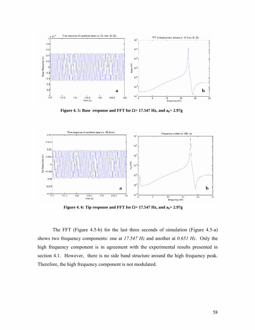
a b
Figure 4. 5: Base response and FFT for Ω= 17.547 Hz, and ab= 2.97g
a b
Figure 4. 6: Tip response and FFT for Ω= 17.547 Hz, and ab= 2.97g
The FFT (Figure 4.5-b) for the last three seconds of simulation (Figure 4.5-a)
shows two frequency components: one at 17.547 Hz and another at 0.651 Hz. Only the
high frequency component is in agreement with the experimental results presented in
section 4.1. However, there is no side band structure around the high frequency peak.
Therefore, the high frequency component is not modulated.
58

Figure 4.6 shows the response and FFT for the tip of the beam. The high and low
frequency components are centered at the same frequencies as the results at the base
(Figure 4.5). However, the amplitude of the low frequency component at the tip of the
beam (Figure 4.6-b) is significantly larger compared to the low frequency component at
the base (Figure 4.5-b).
The FFT's for the numerical results were calculated using Matlab®. For this
calculation, 512 points were sampled from the last three seconds of the time trace
(Figures 4.5-a and 4.6-a). The number of sampled points is a power of 2, thus reducing
the computation time for the FFT (Baher, 1990).
The numerical results show a high frequency component that is not modulated,
and a low frequency component. These results do not agree with the experimental results
obtained by Malatkar (2003). This discrepancy with the experimental results could be
attributed to the presence of numerical error in the calculation of the nonlinear stiffness
matrices kcij and kiij (3.14). Therefore, the numerical error in these matrices is
investigated next.
The nonlinear stiffness matrices are defined in terms of the functions f1 and f2
given by
, ')'''(1 vvf = ∫ ∫∂∂
=s
l
s
dsdsvt
f0
22
2
2 ' (4.2)
In order to investigate the numerical error in the calculation of f1 and f2, these quantities
are calculated for a displacement of the form
txxxxAtxv Ω−−−= sin)]cos(coshsin[sinh),( 111111 ββεββ (4.3)
The bracketed term in (4.3) is simply the first linear mode shape for a cantilever beam
(Appendix B). The constants A1, β1 and ε1 are included in Table B.2. Substituting (4.3)
59
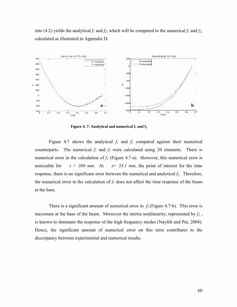
into (4.2) yields the analytical f1 and f2, which will be compared to the numerical f1 and f2,
calculated as illustrated in Appendix D.
a b
Figure 4. 7: Analytical and numerical f1 and f2
Figure 4.7 shows the analytical f1 and f2 compared against their numerical
counterparts. The numerical f1 and f2 were calculated using 20 elements. There is
numerical error in the calculation of f1 (Figure 4.7-a). However, this numerical error is
noticeable for x > 300 mm. At x= 33.1 mm, the point of interest for the time
response, there is no significant error between the numerical and analytical f1. Therefore,
the numerical error in the calculation of f1 does not affect the time response of the beam
at the base.
There is a significant amount of numerical error in f2 (Figure 4.7-b). This error is
maximum at the base of the beam. Moreover the inertia nonlinearity, represented by f2 ,
is known to dominate the response of the high frequency modes (Nayfeh and Pai, 2004).
Hence, the significant amount of numerical error on this term contributes to the
discrepancy between experimental and numerical results.
60

4.3 Transient Response
This section is devoted to the study of the transient response of the cantilever
beam. The finite element model developed in ANSYS® is presented first. The results
from this model are compared to results from the NLB program in Appendix A.
662 mm
y
x
g
0.55 mm
12.71 mm
Beam cross section
nodes
Model Details Total number of elements: 20 Total number of nodes: 21 Length of single element: 33.1 mm BC: All DOF constrained at x= 0 mm
tAaF b Ω= cosρ
Figure 4. 8: Mesh and boundary conditions for ANSYS® model
61

Figure 4.8 shows the geometry used in the finite element model. The vertical
beam has the same dimensions of the beam used by Malatkar (2003) to measure the
experimental steady state response. Moreover, the beam is made of isotropic steel with
properties as listed in section 4.1. The beam is meshed with 20 beam310 elements. Each
element is 33.1 mm long and has section properties calculated using the dimensions in
Figure 4.8.
All degrees of freedom are constrained at the base of the beam (Figure 4.8). This
is consistent with the boundary conditions of the problem (2.60). The effect of gravity is
included in the simulation as shown in Figure 4.8.
The forcing function given by (4.1) is distributed evenly throughout all 21 nodes.
The transient response of the beam is calculated for the first three seconds. The forcing
function given in (4.1) is approximated as a series of straight lines. Figure 4.9 shows the
approximation of one cycle of the forcing function. The cycle of the forcing function is
divided into 14 load steps. This is a reasonable approximation of the exact function
(Figure 4.9). A total of 739 load steps is required to obtain the transient response for the
first three seconds.
Figure 4. 9: Approximation of one cycle of the forcing function
10 ANSYS® Theory Reference, Release 10.0 Documentation for ANSYS®
62

Figure 4.10 shows the response and FFT obtained in ANSYS®. The response plot
(Figure 4.10-a) suggests the presence of multiple frequencies. The FFT11 (Figure 4.10-b)
reveals four frequencies dominating the time response.
a b
Figure 4. 10: Response and FFT from ANSYS®
The four peaks in the FFT (Figure 4.10-b) occur at 0.4798 Hz, 5.518 Hz, 16.07 Hz and
17.51 Hz.
a b
Figure 4. 11: Response and FFT from NLB
11 FFT's were calculated in Matlab® using 512 points sampled from the transient response.
63

Figure 4.11 shows results obtained with NLB. The four frequencies that dominate
the response are centered at 0.7197 Hz, 5.518 Hz, 15.83 Hz, and 17.51 Hz. A combined
plot of the FFT obtained with ANSYS® (Figure 4.12) and the one obtained with NLB
shows both FFT's are in agreement for the most part. The first frequency obtained with
NLB is 50% higher compared to ANSYS®. The remaining three frequencies are
extremely close to the numerical results from NLB. Also, the first mode has a more
significant participation in the time response obtained with ANSYS® (Figure 4.10),
compared to the response obtained with NLB (Figure 4.11).
Figure 4. 12: Combined plot of FFT's
64

Chapter 5: Conclusion and Future Work
5.1 Conclusion
The time response of a vertically mounted, highly flexible, cantilever beam
subjected to harmonic excitation at the base, was investigated. The equation of motion
for the transverse nonlinear vibration of the beam, derived by Crespo da Silva and Glyn
(1978), was solved numerically for the nonlinear displacement using a finite element
model. This finite element model used Galerkin's weighted residuals method combined
with the Newmark technique, and an iterative process, to obtain the nonlinear
displacement of the beam.
The finite element model for the nonlinear transverse vibration of the beam was
implemented in the program NLB12. This program was used to calculate the steady state
response of the beam. The numerical results from the program were compared to the
experimental results obtained by Malatkar (2003). The NLB program was also used to
calculate the transient response of the beam, which was compared with the response
obtained with ANSYS®.
The steady state response for the vertical cantilever beam was measured by
Malatkar (2003) for an excitation frequency of 17.547 Hz, which is close to the third
natural frequency of the beam. The FFT of the experimental results shows a modulated
high frequency component centered at 17.547 Hz, and a low frequency component
centered at 1.58 Hz. Moreover, the modulation frequency for the high frequency
component is equal to the low frequency component, i.e., 1.58 Hz.
The FFT for the steady state response computed with the program NLB shows a
high frequency component centered at 17.547 Hz. Unlike the experimental results from
Malatkar (2003), this high frequency component is not modulated. The absence of
12Non Linear Beam
65

modulation in the high frequency component is attributed to the presence of numerical
error in the computation of the nonlinear inertia term. Nayfeh and Pai (2004) showed
that the nonlinear inertia term dominates the response of the third mode in a highly
flexible beam. The FFT for the numerical results also shows a low frequency component
centered at 0.651 Hz. This result is not in agreement with the experimental results.
The transient response for the first three seconds, obtained with ANSYS® , is
dominated by four frequency components centered at 0.4798 Hz, 5.518 Hz, 16.07 Hz, and
17.51 Hz. The transient response determined with NLB is dominated by frequency
components centered at 0.7197 Hz, 5.518 Hz, 15.83 Hz, and 17.51 Hz. These results are
in agreement with ANSYS® except for the first frequency component, which is 50%
higher with NLB.
In summary, the numerical results obtained with NLB differ from the
experimental results (Malatkar, 2003) due to the presence of numerical error in the
former. The transient response calculated with NLB agrees with the response calculated
with ANSYS® for the most part.
5.2 Future Work
The program NLB needs to be streamlined to reduce computation time of the
steady state response. Also, the numerical error in the calculation of the nonlinear inertia
term should be improved by using alternate numerical methods for its calculation.
66

Bibliography
1 Anderson, T.J., et al., Nonlinear Resonances in a Flexible Cantilever Beam, Nonlinear Vibrations, ASME, Vol. 50, pp. 109-116, 1992
2 Anderson, T.J., et al., Observations of Nonlinear Interactions in a Flexible Cantilever Beam, Proceedings of the 33rd AIAA Structures, Structural Dynamics & Materials Conference, AIAA paper no. 92-2332-CP, Dallas, Tx, pp. 1678-1686
3 ANSYS® Theory Reference, Release 10.0 Documentation for ANSYS® 4 Baher, H., Analog and Digital Signal Processing, John Wiley & Sons, New York,
1990 5 Bathe, K.J., and Wilson, E.L., Stability and Accuracy Analysis of Direct Integration
Methods, Earthquake Engineering and Structural Dynamics, Vol. 1, pp. 283-291, 1973
6 Blevins, R.D., Formulas for Natural Frequency and Mode Shape, Van Nostrand Reinhold Company, New York, 1979
7 Borse, G.J., Numerical Methods with Matlab, PWS-Kent, Boston, 1997 8 Budynas, R.G., Advanced Strength and Applied Stress Analysis, McGraw-Hill,
New York, 1999 9 Cook, R.D., and Young, W.C., Advanced Mechanics of Materials, Prentice Hall,
New Jersey, 1999 10 Cook, R.D., Finite Element Analysis for Stress Analysis, John Wiley & Sons, New
York, 1995 11 Crespo da Silva, M.R.M., and Glynn, C.C., Nonlinear Flexural-Flexural-Torsional
Dynamics of Inextensional Beams. I. Equations of Motion, Journal of Structural Mechanics, Vol. 6, pp. 437-448, 1978
12 Crespo da Silva, M.R.M., and Glynn, C.C., Nonlinear Non-Planar Resonant Oscillations in Fixed-Free Beams with Support Asymmetry, International Journal of Solids Structures, Vol. 15, pp. 209-219, 1979
13 Crespo da Silva, M.R.M., and Glynn, C.C., Out-of Plane Vibrations of a Beam Including Nonlinear Inertia and Non-Linear Curvature Effects, International Journal of Non-Linear Mechanics, Vol. 13, pp. 261-271, 1979
14 Crespo da Silva, M.R.M., and Glynn. C.C., Nonlinear Flexural-Flexural-Torsional Dynamics of Inextensional Beams. II. Forced Motions, Journal of Structural Mechanics, Vol. 6, pp. 449-461, 1978
15 Kim, M.G., et al. Non-planar Nonlinear Vibration Phenomenon on the One to One Internal Resonance of the Circular Cantilever Beam, Key Engineering Materials, Vols. 326-328, pp. 1641-1644, 2006
16 Kreyzig, E., Advanced Engineering Mathematics, John Wiley & Sons, Massachusetts, 1999
17 Love, A.E.H., A Treatise on the Mathematical Theory of Elasticity, Dover Publications, New York, 1944
18 Malatkar, P., and Nayfeh, A.H., On the Transfer of Energy Between Widely Spaced Modes in Structures, Nonlinear Dynamics, Vol. 31, pp. 225-242, 2003
19 Malatkar, P., Nonlinear Vibrations of Cantilever Beams and Plates, Ph.D. thesis, Virginia Polytechnic Institute and State University, 2003
20 Mase, G.E., Continuum Mechanics, McGraw-Hill, New York, 1970
67

21 Meirovitch, L., Fundamentals of Vibrations, McGraw-Hill, New York, 2001 22 Nayfeh, A.H., and Arafat, H.N., Nonlinear response of cantilever beams to
combination and subcombination resonances, Shock and Vibration, Vol. 5, pp. 277-288, 1998
23 Nayfeh, A.H., and Pai, P.F., Linear and Nonlinear Structural Mechanics, John Wiley & Sons, New York, 2003
24 Nayfeh, S.A., and Nayfeh, A.H., Nonlinear Interactions Between Two Widely Spaced Modes- External Excitation, International Journal of Bifurcation and Chaos, Vol. 3, No.2, pp. 417-427, 1993
25 Rao, S.S., Mechanical Vibrations, Addison Wesley, New York, 1990 26 Reddy, J.N., An Introduction to the Finite Element Method, McGraw-Hill, New
York, 1993 27 Thomson, W.T., and Dahleh, M.D., Theory of Vibration with Applications, Prentice
Hall, New Jersey, 1998 28 Török, J.S., Analytical Mechanics, John Wiley & Sons, New York, 2000 29 Zienkiewicz, O.C., A New Look at the Newmark, Houbolt and Other Time Stepping
Formulas. A Weighted Residual Approach, Earthquake Engineering and Structural Dynamics, Vol. 5., pp. 413-418, 1977
30 Zienkiewicz, O.C., The Finite Element Method, McGraw-Hill, London, 1977 31 Zill, D.G., et al., Differential Equations with Boundary Value Problems,
Brooks/Cole Publishing Company, New York, 1997
68

Appendix A: NLB Matlab® Program %Nonlinear Vibration of a Cantilever Beam %Written by Ivan Delgado-Velazquez L= 0.662; W= 0.01271; tk= 5.5e-4; %beam dimensions rho= 7400; E= 165.5e9; %material properties Alpha1= 0.064; Alpha2= 4.72e-5; %proportional damping coefficients N= 20; h= L/N; numX=10; deltax= h/numX; %elements variables TOL=0.01; %convergence criterion for nonlinear loop deltat= 0.001; tf=3; k= tf/deltat; %time variables g=9.81; ab= 2.97*g; OMEGA= 17.547; %force variables Area= W*tk; I= 1/12*W*tk^3; %section properties %shape functions and derivatives xs=0:deltax:h; PSI(:,1)= 1 - (3/h^2)*xs.^2 + (2/h^3)*xs.^3; PSI(:,2)= h*((xs/h) -(2/h^2)*xs.^2 + (1/h^3)*xs.^3); PSI(:,3)= (3/h^2)*xs.^2 - (2/h^3)*xs.^3; PSI(:,4)= h*(-(1/h^2)*xs.^2 + (1/h^3)*xs.^3); PSIP(:,1)= -6*(xs/h^2) + (6/h^3)*xs.^2; PSIP(:,2)= 1 - 4*(xs/h) + (3/h^2)*xs.^2; PSIP(:,3)= 6*(xs/h^2) - (6/h^3)*xs.^2; PSIP(:,4)= - 2*(xs/h) + (3/h^2)*xs.^2; xs4=0:deltax/4:h; PSIP_f2_4(:,1)= -6*(xs4/h^2) + (6/h^3)*xs4.^2; %FOR EVALUATION OF f2 ONLY PSIP_f2_4(:,2)= 1 - 4*(xs4/h) + (3/h^2)*xs4.^2; PSIP_f2_4(:,3)= 6*(xs4/h^2) - (6/h^3)*xs4.^2; PSIP_f2_4(:,4)= - 2*(xs4/h) + (3/h^2)*xs4.^2; PSIPP(:,1)= -6/h^2 + (12/h^3)*xs; PSIPP(:,2)= -4/h + (6/h^2)*xs; PSIPP(:,3)= 6/h^2 - (12/h^3)*xs; PSIPP(:,4)= -2/h + (6/h^2)*xs; PSIPPP(:,1)= (12/h^3)*ones(1,(h/deltax)+1); PSIPPP(:,2)= (6/h^2)*ones(1,(h/deltax)+1); PSIPPP(:,3)= -(12/h^3)*ones(1,(h/deltax)+1); PSIPPP(:,4)= (6/h^2)*ones(1,(h/deltax)+1); Me= (rho*Area*h/420)*[156 22*h 54 -13*h; 22*h 4*h*h 13*h -3*h*h; 54 13*h 156 -22*h; -13*h -3*h*h -22*h 4*h*h]; Ke= (E*I/h^3)*[12 6*h -12 6*h; 6*h 4*h*h -6*h 2*h*h; -12 -6*h 12 -6*h; 6*h 2*h*h -6*h 4*h*h]; Ce= Alpha1*Me + Alpha2*Ke; %element matrices - [M], [KL], [C] Gamma= 0.5; Beta= 0.25; %Newmark coefficients epsilon= 0.5-2*Beta + Gamma; PHI= rho*Area*ab; delta= 0.5 + Beta - Gamma; THETA= 2*pi*OMEGA; %global matrices - [M], [KL], [C] z= 2*(N+1);
69

Mg= zeros(z); Kg= zeros(z); Cg= zeros(z); x1= 1; for x=1:N a=1; for i=x1:x1+3 b=1; for j=x1:x1+3 Mg(i,j)=Mg(i,j)+ Me(a,b); Kg(i,j)=Kg(i,j)+ Ke(a,b); Cg(i,j)=Cg(i,j)+ Ce(a,b); b= b+1; end a= a+1; end x1= x1 +2; end %reduced global matrices for i=1:z-2 for j=1:z-2 MgR(i,j)= Mg(i+2,j+2); KgR(i,j)= Kg(i+2,j+2); CgR(i,j)= Cg(i+2,j+2); end end %Newmark matrices - LINEAR A1= MgR + Gamma*deltat*CgR + Beta*deltat^2*KgR; A2= -2*MgR + (1-2*Gamma)*deltat*CgR + epsilon*deltat^2*KgR; A3= MgR - (1-Gamma)*deltat*CgR + delta*deltat^2*KgR; %Force discretization vector FF= zeros(z,1); a=0; for ll=1:N for aa=1:4 S1=0; S2=0; for l=1:(h/deltax +1) alpha(l)= PSI(l,aa); end for i1=2:2:h/deltax S1= S1 + alpha(i1); end for j1=3:2:h/deltax -1 S2= S2 + alpha(j1); end SS(aa)=(deltax/3)*(alpha(1)+ 4*S1+2*S2+ alpha(h/deltax+1)); end for i1=1:4
70

FF(i1+a)= FF(i1+a) + SS(i1); end a= a+2; for i1=1:z-2 FD(i1,1)= FF(i1+2); end end UL(:,1)= zeros(z,1); %from IC time= 0:deltat:tf; %time vector %Main loop for j=1:k %Linear loop for o=1:z-2 for p=1:j ULr(o,p)= UL(o+2,p); end end if j==1 U0= ULr(:,1); U1= ULr(:,1); F0= zeros(z-2,1); FLin(:,j)= PHI*FD*cos(THETA*time(j)); F1= FLin(:,j); else U0= ULr(:,j-1); U1= ULr(:,j); F0= FLin(:,j-1); F1= FLin(:,j); end FLin(:,j+1)= PHI*FD*cos(THETA*time(j+1)); F2= FLin(:,j+1); F= Beta*F2 + epsilon*F1 + delta*F0; U2= -inv(A1)*A2*U1 - inv(A1)*A3*U0 + deltat^2*inv(A1)*F; ULr(:,j+1)= U2; for i=1:z for p=1:j+1 if i<= 2 UL(i,p)=0; else UL(i,p)= ULr(i-2,p); end end end %Nonlinear loop eps= 10^5; counter= 0; while eps > TOL %first nonlinear stiffness matrix a1= 1; b0= 0; for o=1:N
71

for p= 1:(h/deltax)+1 WWP(p)= PSIP(p,1)*UL(a1,j+1) + PSIP(p,2)*UL(a1+1,j+1)+... PSIP(p,3)*UL(a1+2,j+1) + PSIP(p,4)*UL(a1+3,j+1); WWPP(p)= PSIPP(p,1)*UL(a1,j+1)+ PSIPP(p,2)*UL(a1+1,j+1)+... PSIPP(p,3)*UL(a1+2,j+1) + PSIPP(p,4)*UL(a1+3,j+1); WWPPP(p)= PSIPPP(p,1)*UL(a1,j+1)+ PSIPPP(p,2)*... UL(a1+1,j+1)+PSIPPP(p,3)*UL(a1+2,j+1) + ... PSIPPP(p,4)*UL(a1+3,j+1); WP(p+b0)= WWP(p); WPP(p+b0)= WWPP(p); WPPP(p+b0)= WWPPP(p); end a1= a1+2; b0= b0 + h/deltax; end AA= N*(h/deltax + 1)- N +1; AA_f2_2= N*(2*h/deltax + 1)- N +1; AA_f2_4= N*(4*h/deltax + 1)- N +1; f1= WP.*WPPP + WPP.^2; f1(AA)= 0; %from BC aaa=0; bbb=0; mmm=0; KNL1=zeros(z); for o=1:N for pp=1:4 for qq=1:4 S1=0; S2=0; for l=1:(h/deltax)+1 PsiPijF1(l)= PSIP(l,pp)*PSIP(l,qq)*f1(mmm+l); end for ii=2:2:(h/deltax) S1= S1 + PsiPijF1(ii); end for ii=3:2:(h/deltax - 1) S2= S2 + PsiPijF1(ii); end KKNL(pp,qq)= (deltax/3)*(PsiPijF1(1)+ 4*S1+2*S2 + ... PsiPijF1(h/deltax+1)); KNL1(pp+aaa,qq+bbb)= KNL1(pp+aaa,qq+bbb)+ KKNL(pp,qq); end end aaa= aaa+2; bbb= bbb+2; mmm= mmm + h/deltax; end KNL1= E*I*KNL1; %first nonlinear stiffness matrix for ii=1:z-2 for jj=1:z-2 KNL1r(ii,jj)= KNL1(ii+2,jj+2); %reduced KNL1 end
72

end %second nonlinear stiffness matrix if j == 1 WPsq2Dot= Wpsq2Dot_approx_SS; %approx. with lin. disp. else a1= 1; b0= 0; for o=1:N for p= 1:(4*h/deltax)+1 wWP(p,3)= PSIP_f2_4(p,1)*UL(a1,j+1)+PSIP_f2_4(p,2)*... UL(a1+1,j+1)+PSIP_f2_4(p,3)*UL(a1+2,j+1) +... PSIP_f2_4(p,4)*UL(a1+3,j+1); wWP(p,2)= PSIP_f2_4(p,1)*UL(a1,j) + PSIP_f2_4(p,2)*... UL(a1+1,j)+PSIP_f2_4(p,3)*UL(a1+2,j) +... PSIP_f2_4(p,4)*UL(a1+3,j); wWP(p,1)= PSIP_f2_4(p,1)*UL(a1,j-1)+PSIP_f2_4(p,2)*... UL(a1+1,j-1)+PSIP_f2_4(p,3)*UL(a1+2,j-1) +... PSIP_f2_4(p,4)*UL(a1+3,j-1); wP(p+b0,3)= wWP(p,3); wP(p+b0,2)= wWP(p,2); wP(p+b0,1)= wWP(p,1); end a1= a1+2; b0= b0 + 4*h/deltax; end for ii=1:AA_f2_4 for jj=1:3 WPsq(ii,jj)= wP(ii,jj)*wP(ii,jj); end end for ii=1:AA_f2_4 WPsqDot(ii,1)= (WPsq(ii,2)-WPsq(ii,1))/deltat; WPsqDot(ii,2)= (WPsq(ii,3)-WPsq(ii,2))/deltat; WPsq2Dot(ii)= (WPsqDot(ii,2)-WPsqDot(ii,1))/deltat; end end xx1=1; for xx=1:2:AA_f2_4 S1=0; S2=0; i1=2; j1=3; while i1<= xx-1 S1= S1 + WPsq2Dot(i1); i1= i1 + 2; end while j1<= xx-2 S2= S2 + WPsq2Dot(j1); j1= j1 + 2; end SS1(xx1)=(deltax/12)*(WPsq2Dot(1)+4*S1 + 2*S2 + WPsq2Dot(xx));
73

xx1=xx1+1; end SS1(1)=0; xx2=1; for xx=1:2:AA_f2_2 S1=0; S2=0; i1=xx+1; j1=xx+2; while i1<= AA_f2_2 - 1 S1= S1 + SS1(i1); i1= i1 + 2; end while j1<= AA_f2_2 - 2 S2= S2 + SS1(j1); j1= j1 + 2; end f2(xx2)=(-deltax/6)*(SS1(xx) + 4*S1 + 2*S2 + SS1(AA_f2_2)); xx2=xx2+1; end f2(AA)= 0; aaa=0; bbb=0; mmm=0; KNL2=zeros(z); for o=1:N for pp=1:4 for qq=1:4 S1=0; S2=0; for l=1:(h/deltax)+1 PsiPijF2(l)= PSIP(l,pp)*PSIP(l,qq)*f2(mmm+l); end for ii=2:2:(h/deltax) S1= S1 + PsiPijF2(ii); end for ii=3:2:(h/deltax - 1) S2= S2 + PsiPijF2(ii); end KKnl(pp,qq)= (deltax/3)*(PsiPijF2(1)+ 4*S1+2*S2 + ... PsiPijF2(h/deltax+1)); KNL2(pp+aaa,qq+bbb)= KNL2(pp+aaa,qq+bbb)+ KKnl(pp,qq); end end aaa= aaa+2; bbb= bbb+2; mmm= mmm + h/deltax; end KNL2= 0.5*rho*Area*KNL2; %second nonlinear stiffness matrix for ii=1:z-2 for jj=1:z-2 KNL2r(ii,jj)= KNL2(ii+2,jj+2); %reduced KNL2 end end KTotal= KgR-KNL1r-KNL2r; %total stiffness matrix
74

CNL= Alpha1*MgR + Alpha2*KTotal; %nonlinear damping matrix %nonlinear displacement - Newmark technique for o=1:z-2 for p=1:j UNLr(o,p)= UL(o+2,p); end end if j==1 U0= UNLr(:,1); U1= UNLr(:,1); F0= zeros(z-2,1); FNLin(:,j)= FLin(:,j); F1= FNLin(:,j); else U0= UNLr(:,j-1); U1= UNLr(:,j); F0= FNLin(:,j-1); F1= FNLin(:,j); end %Newmark matrices - NONLINEAR A1NL= MgR + Gamma*deltat*CNL + Beta*deltat^2*KTotal; A2NL= -2*MgR + (1-2*Gamma)*deltat*CNL + epsilon*deltat^2*KTotal; A3NL= MgR - (1-Gamma)*deltat*CNL + delta*deltat^2*KTotal; %total force vector X= 0:deltax:L; %global X vector for ii=1:AA f3(ii)= (X(ii)*deltax - L)*WPP(ii) + WP(ii); end G= zeros(z,1); a=0; m=0; for ll=1:N for aa=1:4 S1=0; S2=0; for l=1:(h/deltax +1) alpha(l)= PSI(l,aa)*f3(m+l); end for i1=2:2:h/deltax S1= S1 + alpha(i1); end for j1=3:2:h/deltax -1 S2= S2 + alpha(j1); end SS(aa)=(deltax/3)*(alpha(1)+ 4*S1+2*S2 + ... alpha(h/deltax+1)); end for i1=1:4 G(i1+a)= G(i1+a) + SS(i1); end a= a+2; m= m+h/deltax;
75

end G= rho*Area*g*G; %gravity vector for i1=1:z-2 Gr(i1)= G(i1+2); end FNLin(:,j+1)= FLin(:,j+1)+ Gr'; %nonlinear force vector F2= FNLin(:,j+1); F= Beta*F2 + epsilon*F1 + delta*F0; U2= -inv(A1NL)*A2NL*U1 - inv(A1NL)*A3NL*U0 + deltat^2*inv(A1NL)*F; UNLr(:,j+1)= U2; for i=1:z for p=1:j+1 if i<= 2 UNL(i,p)=0; else UNL(i,p)= UNLr(i-2,p); end end end for ii=1:z DELTA(ii)= abs(UL(ii,j+1) - UNL(ii,j+1)); end eps= sum(DELTA); UL(:,j+1)= UNL(:,j+1); counter=counter +1; end kounter(j)=counter; %number of iterations in NL loop EPS(j)= eps; %convergence variable for each time step time(j) end %time response plots Response_base= UL(3,:); %response of base (2nd node) Response_tip= UL(z-1,:); %response of tip (last node) figure plot(time,Response_base) xlabel('Time (s)'), ylabel('Base Response (m)') title('Time response of cantilever beam (x=33.1mm)') %figure 1 figure plot(time,Response_tip) xlabel('Time (s)'), ylabel('Tip Response (m)') title('Time response of cantilever beam (x=66.2mm)') %figure 2 %Fast Fourier Transform (FFT) Trecord= 3; %length of time record TI= tf- Trecord; %initial time of sampling TF= tf; %final time of sampling Ta= TI/deltat +1; %element number corresponding to TI
76

Tb= TF/deltat +1; %element number corresponding to TF SR= 6; %sampling rate DELTAT= SR*deltat; %sampling interval fs= 1/(DELTAT); %sampling frequency ii=1; for i=Ta:SR:Tb Response_baseS(ii)= Response_base(i); %sampled points for FFT Response_tipS(ii)= Response_tip(i); %sampled points for FFT ii=ii+1; end Yb= fft(Response_baseS,512); FB= Yb.*conj(Yb); Yt= fft(Response_tipS,512); FT= Yt.*conj(Yt); figure freq = fs*(0:256)/512; plot(freq,FT(1:257)) xlabel('frequency (Hz)'), ylabel('Tip FFT') title('Frequency content of UNL-tip') %figure 3 figure freq = fs*(0:256)/512; plot(freq,FB(1:257)) xlabel('frequency (Hz)'), ylabel('Base FFT') title('Frequency content of UNL-base') %figure 4
77

Appendix B: Linear Natural Frequencies and Mode Shapes
The first four linear mode shapes and natural frequencies for the cantilever beam
in Figure B.1 are calculated next. Both the mode shapes and natural frequencies are
required to calculate the linear forced analytical response of the beam, which is the topic
of Appendix C.
x
y
v(0,t) = 0 v'(0,t) = 0
v"(0,t) = 0 v"'(0,t) = 0
Figure B. 1: Cantilever beam and boundary conditions
The linear equation of motion for the free flexural vibration of the cantilever
beam is given by
0)""( =+ vAEIv &&ρ (B.1)
where E, I, A and ρ are the Young’s modulus, area moment of inertia, cross sectional area
and density, respectively. For uniform properties the equation can be written as
0=+ vEI
Aviv &&ρ (B.2)
Assuming the transverse displacement v is of the form given by
(
tiexVv ω)(= B.3)
here ω is the frequency of vibration, and substituting (B.3) into (B.2) results in w
78

04 =− VV iv β (B.4)
here β is related to E, I, A,ρ , and ω through
w
24 ωρβEI
A= (B.5)
Equation (B.4) is a linear ordinary differential equation with constant coefficients.
hus, the characteristic equation of (B.4) is (Kreyszig, 1999)
T
xDxCxBxAxV ββββ cossincoshsinh)( +++= (B.6)
, and D are constants. The first three derivatives o
where A, B, C f (B.6) are
xDxCxBxAxV
xDxCxBxAxVxDxCxBxAxV
ββββββββ
ββββββββ
ββββββββ
sincossinhcosh)('''cossincoshsinh)("3333
2222
+−+=
−−+=
sincossinhcosh)(' −++=
(B.7)
Substituting the boundary conditions listed in Figure B.1 into equations (B.6) and (B.7)
yields
DB −= , CA −= (B.8)
AB)cos(cosh)sin(sinh
θθθθ
++−
= (B.9)
.6) through (B.9) yields
(B.10)
here θ is the product βl. Moreover, substituting (B.8) into (B.6) results in
Further manipulation of equations (B
θθ 1coshcos −−=
w
79

))cos()(cosh((sinh)( xxBAxV ))sin()( xx β βββ −+−= (B
.11)
eam.
Figure (B.2)
ows a plot of both sides of equation (B.10). The natural frequencies are calculated
of θ where both curves intersect.
Figure
ilever beam
Equation (B.10) is solved graphically for the natural frequencies of the b
This is done by plotting both sides of the equation against the variable θ.
sh
from the values
B. 2: Plot used to obtain natural frequencies
Table B. 1: Natural frequencies of linear cant
Mode number ) fn - exact (Hz) θ (rad) fn- graphical (Hz
1 1.88 0.96 0.959
2 4.7 6.02 6.008
3 7.85 16.8 16.824
4 11 33 32.961
The natural frequencies obtained from equation (B.10) are presented in Table B.1.
These na l frequencies are c red against the exact values provided by Rao (1990).
The frequencies obtained from (B.10) are extremely clo o the exact frequ
tura ompa
se t encies.
80

The mode shapes of the cantilever beam are obtained by substituting (B.9) into
.11), along with the appropriate θ from Table B.1. Thus, the rth mode shape is given
y
B.12)
(B
b
)]cos(coshsin[sinh)(* xxxxAxV rrrrrrr ββεββ −−−= (
with εr given by
)cos(cosh)sin(sinh
rr
rrr θθ
θθε++−
= (B.13)
xr indicates the mode shape is normalized.
(Meirovitch, 2001)
rr dxVAV0
1ρ (B.14)
he density and cross sectional area, respectively. Substituting (B.12)
to (B.14) and solving for Ar yields
The asterisk in *V )(
The constants Ar in (B-12) are obtained using the orthogonality relation given by
∫ =l
**
where ρ and A are t
in
rr AI
Aρ
1= (B.15)
gral
rr0
c)n( εβ − B.16)
where the quantity Ir is simply the inte
dxxxxI rrr
l
rr2))cos()osh(si)(sinh( βεββ +−= ∫ (
x
81

he values of Ar, βr, and εr for the first four modes are included in Table B.2. These
rced response of the beam in terms of the
rst four mode shapes.
Table B. 2: Constants for the first four mode shapes
T
values are used in Appendix C to write the fo
fi
r Ar βr εr
1 3.967 2.84 1.36
2 5.504 7.1 0.982
3 5.4 11.86 1
4 5.404 16.62 1
82

Appendix C: Forced Vibration of a Cantilever Beam
The forced response of a cantilever beam subjected to harmonic excitation at the
se (Figure C.1) is presented next. The cantilever beam is made of isotropic material
properties.
Figure C. 1: Cantilever beam subjected to base excitation
From Appendix B, the linear equation of motion in the y direction is given by
ba
and has uniform
y
x V(t)
0)""( =+ vAEIv &&ρ (C.1)
he displacement V(t) applied to the base of the beam in the
direction is given by
where E, I, ρ, and A are the Young's modulus, area moment of inertia, density and cross
sectional area, respectively. T
y
)cos()( 0 tvtV Ω=
.2)
her v0 is the maximum amplitude of the displacement at the base, and Ω the excitation
am is given by
(C
w
frequency. The transverse displacement v of any point along the be
)(tVvv b += (C.3)
83

where vb is the displacement of the beam relative to the base. Substituting (C.3) into (C.1)
hich can be written as
(C.5)
forcing
nction f(x,t) in (C.5) is given by
yields
0))cos(( 20 =ΩΩ−+ tvvAEIv b
ivb &&ρ (C.4)
w
),( txfvAEIviv =+ &&ρ
Equation (C.5) is a partial differential equation in the displacement relative to the base of
the beam vb. However, the subscript b is dropped for the sake of simplicity. The
fu
tAatxf b Ω= cos),( ρ (C.6)
ab is the m the beam,
(C.7)
tem for the problem
igure C.2.
Figure C. 2: Cantilever beam with boundary conditions
where aximum amplitude of the acceleration applied to the base of
and is given by
20Ω= vab
The dynamic sys described by equation (C.5) is shown in
F
f(x,t)
x
y
v(0,t) = 0 v'(0,t) = 0
v"(0,t) = 0 v"'(0,t) = 0
84

The transverse displacement relative se of the beam is assumed as to the ba
∑=r
rr tqxVtxv )()(),( * (C.8)
where )(* xVr are the normalized mode shapes derived in Appendix B. Substituting (C.8)
to (C.5) , multiplying the resulting expression by , and integrating over the
ngth of the beam results in
(C.9)
son, 1998)
** =∫ , (C.10)
here δrs is the Kronecker delta. Substituting (C.10) into (C.9) yields
ith Qr(t) given by
rrr thQtbtatq0
()())sin()( τωω C.13)
)(* xVsin
le
∫∫∫ =+l
srr
l
s
l
riv
rs dxtxfVqdxVVAqdxVVEI0
**
0
*
0
** ),(][][ &&ρ
The mode shapes are orthonormal and obey the following relations (Thom
rsr
liv
rs dxVVEI δω 2rsr
l
s dxVVA δρ =∫ *
0
* 0
w
)(2 tQqq rrrr =+ &&ω (C.11)
w
(C.12) ∫=l
rr dxtxfVtQ0
* ),()(
The solution of (C.11) is given by (Zill, 1997)
r d)cos( ττ (
∫ −++=t
rr
85

where the third term is (C.13) is the convolution integral (Thomson, 1998). The quantity
and is given by
h(t-τ) in the third term of (C.13) is the unit impulse response of (C.11)
)](sin[1)( τωω
τ −=− tth rr
(C.14)
nd (C.12) into the convolution integral yields
Substituting (C.14) a
∫ ∫ ∫ =−Ω=−t
rrl t
rrr
br FFdttdxVAadthQ
021
0 0
* )(sin[)cos()()( ττωω
ρτττ (C.15)
ith
l
rdxV0
* ,
w r and rF2 defined as F1
∫ ∫ −Ω=t
rr
br dttAaF0
2 )(sin[)cos( ττωω
ρ =rF1 (C.16)
The initial conditions for this problem are given by
, 0)0,( =xv&0)0,( =xv (C.17)
ubstituting (C.17) into (C.13) yields
,
S
0=ra ])(2
1)(2
1[1 Ω++
Ω−−=
rrr
brr
AaFbωωω
ρ
(C.19)
nd the beam response is obtained by substituting (C.19) into (C.13).
(C.18)
Therefore qr is given by
rr
rrr FFtbtq 21)cos()( += ω
a
86

Appendix D: Cal oculation f kiij
late the inertial nonlinear stiffness matrix is
lustrated through a simple example. A similar procedure is used to calculate the
stiffn matrix and the gravitational effec
sh for cantilever beam
en
t. he nodal
isplacements Qj (j=1...6) were obtained using the Newmark technique discussed in
ction 3.3.1.
Recall from Chapter 3, the inertial nonlinear stiffness matrix (3.14) is defined
terms of the function f2 , which is given by
ijki The procedure used to calcu
il
curvature nonlinear ess t vector ig . ijkc ,
Figure D. 1: Two-element me
For this example a cantilever beam of length l is meshed with two elem ts
(Figure D.1) of length h each. Moreover, each element is divided into five smaller
divisions of length Δx, resulting in a total of six grid points per elemen T
d
se
ijki
in
s
Δx
y 2 3 4 5 7 8 9 101 6 11
Q1, Q2 Q3, Q4 Q5, Q6
h
1s 11s
l
87

∫ ∫∂∂
=s
l
s
dsdsvt
f0
22
2
2 ' (D.1)
here v is the transverse displacement in the y direction (Figure D.1). The order of
ifferentiation and integration in (D.1) can be reversed, since these operators conmute
w
d
(Kreyszig, 1999). Hence, f2 is written as
∫ ∫ ∂∂
=s
l
s
dsdstvf
02
22
2' (D.2)
Equation (D.2) is evaluated numerically in three steps. The second derivative of
v'2 with respect to time is calculated first, followed by the first integral from 0 to s, and
l to s. These steps are discussed in detail next.
the spatial derivative of the transverse
isplacement v needs to be estimated. The transverse displacement is approximated as
≈2
),(~e tsVv (D.3)
he element given by
4
1= ∑
=
tQsj
ejjψ
finally the second integral from
In order to evaluate f2 using (D.2)
d
∑=1e
where ),(~ tsV e is the displacement inside t
2,1),(~=etsV e (D.4) )()(
with the shape functions given by (Reddy, 1993)
32
⎞⎛⎞⎛ ss1 231 ⎟
⎠⎜⎝
+⎟⎠
⎜⎝
−=hh
ψ , ⎥⎥⎦
⎤⎡ ⎞⎛⎞⎛⎞⎛32 sss
⎢⎢⎣
⎟⎠
⎜⎝
+⎟⎠
⎜⎝
−⎟⎠
⎜⎝
=2 2hhh
h , ψ
32
3 23 ⎟⎞
⎜⎛−⎟
⎞⎜⎛=
ss⎠⎝⎠⎝ hh
ψ , ⎥⎥⎤
⎢⎡
⎟⎞
⎜⎛+⎟
⎞⎜⎛−=
32
4ssh
⎦⎢⎣ ⎠⎝⎠⎝ hhψ (D.5)
88

Substituting (D.4) into (D.3) yields
≈2 4
)()( e tQsv ψ (D.6)
which is used to calculate the spatial derivative of the transverse displacement.
∑∑= =1 1e j
jj
∑∑∂
= = ∂≈
2 4
)()(
' ej
j tQs
v1 1e j s
ψ (D.7)
The second time derivative of v'2 in the interval [0,TF] ,where TF is an arbitrary
ulated next. Figure D. ows the time nodes in the interval [0,TF], where j
is the time node index.
Figure D. 2: Time nodes in [0,TF]
time, is calc 2 sh
Δt 2Δt
The number of time nodes in [0,TF] is given by
1+Δ
=t
TFTN (D.8)
time derivative of v'2 is given by
The second derivative of v'2 with respect to time for an arbitrary node in [0,TF],
such that 1 < j < TN , is calculated using the central difference formula (Kreyszig,
1999). Thus, the second
2
11
2
22 ''2'')(t
vvvtvsJ
jjj
jj Δ
+−=
∂∂
=−+
(D.9)
5 ... 2 j= 1 TN 3 4
t=0 3Δt 4Δt (j-1)Δt = TF
89

where '1vj+ , 'vj and '1vj− are the values of the function v' evaluated at time nodes j+1, j,
nd j-1 espectively.
time of v'2 for node 1 in [0,TF] is
pproximated using the linear transverse transient displacement solution of a cantilever
rrrrr tFFtbsVtsv )]()cos()[(),( 21
* ω (D.10)
iven by (B.12). The quantities
r, , and are defined in Appendix C. The second derivative of v'2 with respect
=1) in [0,TF] is then
a , r
The second derivative with respect to
a
beam given by
∑ +=r
The rV* are the normalized modes for the linear problem grF1 )(2 tF rb
to time for node 1 ( j
1))'(''(2')( 2 2∂t jj
22
=+=∂
= jvvvvsJ &&& (D.11)
s of v.
ed, f2 is given by
(D.12)
Notice the subscript has been omitted in (D.12) for the sake of simplicity. Equation
ated next.
For any grid point along the beam, f2 is given by
where (D.10) is used to calculate the required derivative
Now that the expressions for the second time derivative of v'2 for all the nodes in
[0,TF] are defin
∫ ∫=s
l
s
dsdssJf0
2 )(
j
(D.12) is evaluated numerically for all eleven grid points along the beam (Figure D.1).
The numerical integration of (D.12) is illustr
90

(D.13)
here sk is the kth grid point in Figure D.1; and a is the total number of grid points along
n (D.13) is calculated as (Borse, 1997)
akdsdssJsfk ks
l
s
k ...1)()(0
2 == ∫ ∫
w
the beam, eleven for this example. Both integrals in (D.13) are evaluated using
Simpson's rule. The first integral i
)]()(2)()()(21
1 k
k
i
k
ik sJsJsJdssJsIk
++== ∑∑∫−−
(D.14) 4)0([)1(3 320
ioddi
ieveni
ks
Jks
+− ==
Finally, f2 is calculated as (Borse, 1997)
)]()(2)(4)([)(3
)()( 1
2
21
1
11112 k
ka
ioddi
ik
ka
ieven
l =iik
kk sIsIsIlI
kalsdssIsf +++
−−
== ∑∑∫−−
=++ (D.15)
The function f2 given by (D.13) is finally used to calculate the element inertial
s
sk −−
nonlinear stiffness matrice
60
21 0)(''
21 ssdssfAki
h
ji <<= ∫ ψψρ (D.16)
ij
lssdssfAkih
<<= ∫2 )(''1 ψψρ jiij 60
22 (D.17)
where , A, and l are the density, cross sectional area, and length of the beam,
tively. The range for s in (D.16) and (D.17) is defined from Figure D.1. Assembly
.17) yields the global inertial nonlinear
fness matrix kiij. The integration in (D.16) and (D.17) is done using Simpson's rule.
ρ
respec
of the two element matrices (D.16) and (D
stif
91