Nonlinear Time Series in FinancialForecasting�

Gloria González-RiveraDepartment of Economics

University of California, RiversideRiverside, CA 92521-0427

E-mail: gloria.gonzalez@ucr.eduphone: +1 951-827-1470fax +1 951-827-5685

Tae-Hwy LeeDepartment of Economics

University of California, RiversideRiverside, CA 92521-0427E-mail: taelee@ucr.eduphone: +1 951-827-1509fax +1 951-827-5685

First Version: September 2007This Version: February 2008

�We would like to thank Bruce Mizrach for useful comments. All errors are our own. Entry ID 00221for Encyclopedia of Complexity and System Science. Publisher contact: Julia.Koerting@springer.com, Ker-stin.Kindler@springer.com. Editor: Bruce Mizrach <mizrach@economics.rutgers.edu>. Project website:http://refworks.springer.com/complexity

1

Article Outline

Glossary

1. De�nitions

2. Introduction

3. Nonlinear forecasting models for the conditional mean

4. Nonlinear forecasting models for the conditional variance

5. Forecasting beyond mean and variance

6. Evaluation of nonlinear forecasts

7. Conclusions

8. Future directions

9. Bibliography

2

Glossary

Arbitrage Pricing Theory (APT): the expected return of an asset is a linear functionof a set of factors.Arti�cial neural network: is a nonlinear �exible functional form, connecting inputs to

outputs, being capable of approximating a measurable function to any desired level of accu-racy provided that su¢ cient complexity (in terms of number of hidden units) is permitted.Autoregressive Conditional Heteroskedasticity (ARCH): the variance of an asset

returns is a linear function of the past squared surprises to the asset.Bagging: short for bootstrap aggregating. Bagging is a method of smoothing the pre-

dictors�instability by averaging the predictors over bootstrap predictors and thus loweringthe sensitivity of the predictors to training samples. A predictor is said to be unstable ifperturbing the training sample can cause signi�cant changes in the predictor.Capital Asset Pricing Model (CAPM): the expected return of an asset is a linear

function of the covariance of the asset return with the return of the market portfolio.Factor model: a linear factor model summarizes the dimension of a large system of

variables by a set of factors that are linear combinations of the original variables.Financial forecasting: prediction of prices, returns, direction, density or any other

characteristic of �nancial assets such as stocks, bonds, options, interest rates, exchangerates, etc.Functional coe¢ cient model: a model with time-varying and state-dependent coe¢ -

cients. The number of states can be in�nite.Linearity in mean: the process fytg is linear in mean conditional on Xt if

Pr [E(ytjXt) = X 0t��] = 1 for some �� 2 Rk:

Loss (cost) function: When a forecast ft;h of a variable Yt+h is made at time t forh periods ahead, the loss (or cost) will arise if a forecast turns out to be di¤erent fromthe actual value. The loss function of the forecast error et+h = Yt+h � ft;h is denoted asct+h(Yt+h; ft;h); and the function ct+h(�) can change over t and the forecast horizon h:Markov-switching model: features parameters changing in di¤erent regimes, but in

contrast with the threshold models the change is dictated by a non-observable state variablethat is modelled as a hidden Markov chain.Martingale property: tomorrow�s asset price is expected to be equal to today�s price

given some information setE(pt+1jFt) = pt

3

Nonparametric regression: is a data driven technique where a conditional moment ofa random variable is speci�ed as an unknonw function of the data and estimated by meansof a kernel or any other weighting scheme on the data.Random �eld: a scalar random �eld is de�ned as a function m(!; x) : �A! R such

that m(!; x) is a random variable for each x 2 A where A � Rk:

Sieves: the sieves or approximating spaces are approximations to an unknown function,that are dense in the original function space. Sieves can be constructed using linear spansof power series, e.g., Fourier series, splines, or many other basis functions such as arti�cialneural network (ANN), and various polynomials (Hermite, Laguerre, etc.).Smooth transition models: threshold model with the indicator function replaced by

a smooth monotonically increasing di¤erentiable function such as a probability distributionfunction.Threshold model: a nonlinear model with time-varying coe¢ cients speci�ed by using

an indicator which takes a non-zero value when a state variable falls on a speci�ed partitionof a set of states, and zero otherwise. The number of partitions is �nite.Varying Cross-sectional Rank (VCR): of asset i is the proportion of assets that

have a return less than or equal to the retunr of �rm i at time t

zi;t �M�1MXj=1

1(yj;t � yi;t)

Volatility: Volatility in �nancial economics is often measured by the conditional vari-ance (e.g., ARCH) or the conditional range. It is important for any decision making underuncertainty such as portfolio allocation, option pricing, risk management.

4

1 De�nitions

1.1 Financial forecasting

Financial forecasting is concerned with the prediction of prices of �nancial assets such as

stocks, bonds, options, interest rates, exchange rates, etc. Though many agents in the econ-

omy, i.e. investors, money managers, investment banks, hedge funds, etc. are interested

in the forecasting of �nancial prices per se, the importance of �nancial forecasting derives

primarily from the role of �nancial markets within the macro economy. The development

of �nancial instruments and �nancial institutions contribute to the growth and stability of

the overall economy. Because of this interconnection between �nancial markets and the real

economy, �nancial forecasting is also intimately linked to macroeconomic forecasting, which

is concerned with the prediction of macroeconomic aggregates such as growth of the gross

domestic product, consumption growth, in�ation rates, commodities prices, etc. Finan-

cial forecasting and macroeconomic forecasting share many of the techniques and statistical

models that will be explained in detail in this article.

In �nancial forecasting a major object of study is the return to a �nancial asset, mostly

calculated as the continuously compounded return, i.e., yt = log pt � log pt�1 where pt is theprice of the asset at time t. Nowadays �nancial forecasters use sophisticated techniques that

combine the advances in modern �nance theory, pioneered by Markowitz (1959), with the

advances in time series econometrics, in particular the development of nonlinear models for

conditional moments and conditional quantiles of asset returns.

The aim of �nance theory is to provide models for expected returns taking into account

the uncertainty of the future asset payo¤s. In general, �nancial models are concerned with

investors�decisions under uncertainty. For instance the portfolio allocation problem deals

with the allocation of wealth among di¤erent assets that carry di¤erent levels of risk. The

implementation of these theories relies on econometric techniques that aim to estimate �-

nancial models and testing them against the data. Financial econometrics is the branch of

econometrics that provides model-based statistical inference for �nancial variables, and there-

fore �nancial forecasting will provide their corresponding model-based predictions. However

there are also econometric developments that inform the construction of ad hoc time series

5

models that are valuable on describing the stylized facts of �nancial data.

Since returns fytg are random variables, the aim of �nancial forecasting is to forecast

conditional moments, quantiles, and eventually the conditional distribution of these variables.

Most of the time our interest will be centered on expected returns and volatility as these

two moments are crucial components on portfolio allocation problems, option valuation,

and risk management, but it is also possible to forecast quantiles of a random variable,

and therefore to forecast the expected probability density function. Density forecasting is

the most complete forecast as it embeds all the information on the �nancial variable of

interest. Financial forecasting is also concerned with other �nancial variables like durations

between trades and directions of price changes. In these cases, it is also possible to construct

conditional duration models and conditional probit models that are the basis for forecasting

durations and market timing.

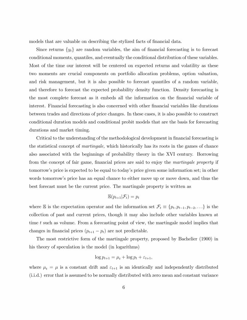
Critical to the understanding of the methodological development in �nancial forecasting is

the statistical concept of martingale, which historically has its roots in the games of chance

also associated with the beginnings of probability theory in the XVI century. Borrowing

from the concept of fair game, �nancial prices are said to enjoy the martingale property if

tomorrow�s price is expected to be equal to today�s price given some information set; in other

words tomorrow�s price has an equal chance to either move up or move down, and thus the

best forecast must be the current price. The martingale property is written as

E(pt+1jFt) = pt

where E is the expectation operator and the information set Ft � fpt; pt�1; pt�2; : : :g is thecollection of past and current prices, though it may also include other variables known at

time t such as volume. From a forecasting point of view, the martingale model implies that

changes in �nancial prices (pt+1 � pt) are not predictable.

The most restrictive form of the martingale property, proposed by Bachelier (1900) in

his theory of speculation is the model (in logarithms)

log pt+1 = �t + log pt + "t+1;

where �t = � is a constant drift and "t+1 is an identically and independently distributed

(i.i.d.) error that is assumed to be normally distributed with zero mean and constant variance

6

�2. This model is also known as a random walk model. Since the return is the percentage

change in prices, i.e. yt = log pt � log pt�1, an equivalent model for asset returns is

yt+1 = �t + "t+1:

Then, taking conditional expectations, we �nd that E(yt+1jFt) = �t. If the conditional

mean return is not time-varying, �t = �, then the returns are not forecastable based on

past price information. In addition and given the assumptions on the error term, returns are

independent and identically distributed random variables. These two properties, a constant

drift and an i.i.d error term, are too restrictive and they rule out the possibility of any

predictability in asset returns. A less restrictive and more plausible version is obtained when

the i.i.d assumption is relaxed. The error term may be heteroscedastic so that returns have

di¤erent (unconditional or conditional) variances and consequently they are not identically

distributed, and/or the error term, though uncorrelated, may exhibit dependence in higher

moments and in this case the returns are not independent random variables.

The advent of modern �nance theory brings the notion of systematic risk, associated with

return variances and covariances, into asset pricing. Though these theories were developed

to explain the cross-sectional variability of �nancial returns, they also helped many years

later with the construction of time series models for �nancial returns. Arguably, the two

most important asset pricing models in modern �nance theory are the Capital Asset Pricing

Model (CAPM) proposed by Sharpe (1964) and Lintner (1965) and the Arbitrage Pricing

Theory (APT) proposed by Ross (1976). Both models claim that the expected return to

an asset is a linear function of risk; in CAPM risk is related to the covariance of the asset

return with the return to the market portfolio, and in APT risk is measured as exposure to

a set of factors, which may include the market portfolio among others. The original version

of CAPM, based on the assumption of normally distributed returns, is written as

E(yi) = yf + �im [E(ym)� yf ] ;

where yf is the risk-free rate, ym is the return to the market portfolio, and �im is the risk of

asset i de�ned as

�im =cov(yi; ym)

var(ym)=�im�2m

:

7

This model has a time series version known as the conditional CAPM (Bollerslev, Engle,

and Wooldridge, 1988) that it may be useful for forecasting purposes. For asset i and given

an information set as Ft = fyi;t; yi;t�1; : : : ; ym;t; ym;t�1; : : :g, the expected return is a linearfunction of a time-varying beta

E(yi;t+1jFt) = yf + �im;t [E(ym;t+1jFt)� yf ]

where �im;t =cov(yi;t+1;ym;t+1jFt)var(ym;t+1jFt) =

�im;t�2m;t

: From this type of models is evident that we need

to model the conditional second moments of returns jointly with the conditional mean. A

general �nding of this type of models is that when there is high volatility, expected returns

are high, and hence forecasting volatility becomes important for the forecasting of expected

returns. In the same spirit, the APT models have also conditional versions that exploit the

information contained in past returns. A K-factor APT model is written as

yt = c+B0ft + "t;

where ft is a K� 1 vector of factors and B is a K �1 vector of sensitivities to the factors. Ifthe factors have time-varying second moments, it is possible to specify an APT model with

a factor structure in the time-varying covariance matrix of asset returns (Engle, Ng, and

Rothschild, 1990), which in turn can be exploited for forecasting purposes.

The conditional CAPM and conditional APT models are �ne examples on how �nance

theory provides a base to specify time-series models for �nancial returns. However there

are other time series speci�cations, more ad hoc in nature, that claim that �nancial prices

are nonlinear functions �not necessarily related to time-varying second moments� of the

information set and by that, they impose some departures from the martingale property.

In this case it is possible to observe some predictability in asset prices. This is the subject

of nonlinear �nancial forecasting. We begin with a precise de�nition of linearity versus

nonlinearity.

1.2 Linearity and nonlinearity

Lee, White, and Granger (LWG, 1993) are the �rst who precisely de�ne the concept of

"linearity". Let fZtg be a stochastic process, and partition Zt as Zt = (yt X 0t)0, where (for

8

simplicity) yt is a scalar and Xt is a k� 1 vector. Xt may (but need not necessarily) contain

a constant and lagged values of yt. LWG de�ne that the process fytg is linear in meanconditional on Xt if

Pr [E(ytjXt) = X 0t��] = 1 for some �� 2 Rk:

In the context of forecasting, Granger and Lee (1999) de�ne linearity as follows. De�ne

�t+h = E(yt+hjFt) being the optimum least squares h-step forecast of yt+h made at time t.

�t+h will generally be a nonlinear function of the contents of Ft: Denote mt+h the optimum

linear forecast of yt+h made at time t be the best forecast that is constrained to be a

linear combination of the contents of Xt 2 Ft: Granger and Lee (1999) de�ne that fytgis said to be linear in conditional mean if �t+h is linear in Xt, i.e., Pr

��t+h = mt+h

�= 1

for all t and for all h. Under this de�nition the focus is the conditional mean and thus a

process exhibiting autoregressive conditional heteroskedasticity (ARCH) (Engle,1982) may

nevertheless exhibit linearity of this sort because ARCH does not refer to the conditional

mean. This is appropriate whenever we are concerned with the adequacy of linear models for

forecasting the conditional mean returns. See White (2006, Section 2) for a more rigorous

treatment on the de�nitions of linearity and nonlinearity.

This de�nition may be extended with some caution to the concept of linearity in higher

moments and quantiles, but the de�nition may depend on the focus or interest of the re-

searcher. Let "t+h = yt+h � �t+h and �2t+h = E("2t+hjFt): If we consider the ARCH and

GARCH as linear models, we say��2t+h

is linear in conditional variance if �2t+h is a linear

function of lagged "2t�j and �2t�j for some h or for all h: Alternatively, �

2t+h = E("2t+hjFt) is

said to be linear in conditional variance if �2t+h is a linear function of xt 2 Ft for some h orfor all h: Similarly, we may consider linearity in conditional quantiles. The issue of linearity

versus nonlinearity is most relevant for the conditional mean. It is more relevant whether a

certain speci�cation is correct or incorrect (rather than linear or nonlinear) for higher order

conditional moments or quantiles.

9

2 Introduction

There exists a nontrivial gap between martingale di¤erence and serial uncorrelatedness.

The former implies the latter, but not vice versa. Consider a stationary time series fytg:Often, serial dependence of fytg is described by its autocorrelation function �(j); or by itsstandardized spectral density

h(!) =1

2�

1Xj=�1

�(j)e�ij!; ! 2 [��; �]:

Both h(!) and �(j) are the Fourier transform of each other, containing the same information

of serial correlations of fytg: A problem with using h(!) and �(j) is that they cannot cap-

ture nonlinear time series that have zero autocorrelation but are not serially independent.

Nonlinear MA and Bilinear series are good examples:

Nonlinear MA : Yt = bet�1et�2 + et;

Bilinear : Yt = bet�1Yt�2 + et:

These processes are serially uncorrelated, but they are predictable using the past informa-

tion. Hong and Lee (2003a) note that the autocorrelation function, the variance ratios,

and the power spectrum can easily miss these processes. Misleading conclusions in favor of

the martingale hypothesis could be reached when these test statistics are insigni�cant. It

is therefore important and interesting to explore whether there exists a gap between ser-

ial uncorrelatedness and martingale di¤erence behavior for �nancial forecasting, and if so,

whether the neglected nonlinearity in conditional mean can be explored to forecast �nancial

asset returns.

In the forthcoming sections, we will present, without being exhaustive, nonlinear time

series models for �nancial returns, which are the basis for nonlinear forecasting. In Section

3, we review nonlinear models for the conditional mean of returns. A general representation

is yt+1 = �(yt; yt�1; :::) + "t+1 with �(�) a nonlinear function of the information set. If

E(yt+1jyt; yt�1; :::) = �(yt; yt�1; :::), then there is a departure from the martingale hypothesis,

and past price information will be relevant to predict tomorrow�s return. In Section 4, we

review models for the conditional variance of returns. For instance, a model like yt+1 =

10

� + ut+1�t+1 with time-varying conditional variance �2t+1 = E((yt+1 � �)2jFt) and i.i.d.error ut+1, is still a martingale-di¤erence for returns but it represents a departure from the

independence assumption. The conditional mean return may not be predictable but the

conditional variance of the return will be. In addition, as we have seen modeling time-

varying variances and covariances will be very useful for the implementation of conditional

CAPM and APT models.

3 Nonlinear forecasting models for the conditional mean

We consider models to forecast the expected price changes of �nancial assets and we restrict

the loss function of the forecast error to be the mean squared forecast error (MSFE). Under

this loss, the optimal forecast is �t+h = E(yt+hjFt). Other loss functions may also be usedbut it will be necessary to forecast other aspects of the forecast density. For example, under

a mean absolute error loss function the optimal forecast is the conditional median.

There is evidence for �t+h being time-varying. Simple linear autoregressive polynomials

in lagged price changes are not su¢ cient to model �t+h and nonlinear speci�cations are

needed. These can be classi�ed into parametric and nonparametric. Examples of parametric

models are autoregressive bilinear and threshold models. Examples of nonparametric models

are arti�cial neural network, kernel and nearest neighbor regression models.

It will be impossible to have an exhaustive review of the many nonlinear speci�cations.

However, as discussed in White (2006) and Chen (2006), some nonlinear models are univer-

sal approximators. For example, the sieves or approximating spaces are proven to approx-

imate very well unkown functions and they can be constructed using linear spans of power

series, Fourier series, splines, or many other basis functions such as arti�cial neural net-

work (ANN), Hermite polynomials as used in e.g., Gallant and Nychka (1987) for modelling

semi-nonparametric density, and Laguerre polynomials used in Nelson and Siegel (1987) for

modelling the yield curve. Diebold and Li (2006) and Huang, Lee, and Li (2007) use the

Nelson-Siegel model in forecasting yields and in�ation.

We review parametric nonlinear models like threshold model, smooth transition model,

Markov switching model, and random �elds model; nonparametric models like local linear,

11

local polynomial, local exponential, and functional coe¢ cient models; and nonlinear models

based on sieves like ANN and various polynomials approximations. For other nonlinear

speci�cations we recommend some books on nonlinear time series models such as Fan and

Yao (2003), Gao (2007), Tsay (2005). We begin with a very simple nonlinear model.

3.1 A simple nonlinear model with dummy variables

Goyal and Welch (2006) forecast the equity premium on the S&P 500 index �index return

minus T-bill rate� using many predictors such as stock-related variables (e.g., dividend-

yield, earning-price ratio, book-to-market ratio, corporate issuing activity, etc.), interest-

rate-related variables (e.g., treasury bills, long-term yield, corporate bond returns, in�ation,

investment to capital ratio), and ex ante consumption, wealth, income ratio (modi�ed from

Lettau and Ludvigson 2001). They �nd that these predictors have better performance in

bad times, such as the Great Depression (1930-33), the oil-shock period (1973-75), and the

tech bubble-crash period (1999-2001). Also, they argue that it is reasonable to impose a

lower bound (e.g., zero or 2%) on the equity premium because no investor is interested in

(say) a negative premium.

Campbell and Thompson (2007), inspired by the out-of-sample forecasting of Goyal and

Welch (2006), argue that if we impose some restrictions on the signs of the predictors�

coe¢ cients and excess return forecasts, some predictors can beat the historical average equity

premium. Similarly to Goyal and Welch (2006), they also use a rich set of forecasting

variables � valuation ratios (e.g., dividend price ratio, earning price ratio, and book to

market ratio), real return on equity, nominal interest rates and in�ation, and equity share

of new issues and consumption-wealth ratio. They impose two restrictions �the �rst one

is to restrict the predictors�coe¢ cients to have the theoretically expected sign and to set

wrong-signed coe¢ cients to zero, and the second one is to rule out a negative equity premium

forecast. They show that the e¤ectiveness of these theoretically-inspired restrictions almost

always improve the out-of sample performance of the predictive regressions. This is an

example where "shrinkage" works, that is to reduce the forecast error variance at the cost

of a higher forecast bias but with an overall smaller mean squared forecast error (the sum of

12

error variance and the forecast squared bias).

The results from Goyal and Welch (2006) and Campbell and Thompson (2007) support

a simple form of nonlinearity that can be generalized to threshold models or time-varying

coe¢ cient models, which we consider next.

3.2 Threshold models

Many �nancial and macroeconomic time series exhibit di¤erent characteristics over time

depending upon the state of the economy. For instance, we observe bull and bear stock

markets, high volatility versus low volatility periods, recessions versus expansions, credit

crunch versus excess liquidity, etc. If these di¤erent regimes are present in economic time

series data, econometric speci�cations should go beyond linear models as these assume that

there is only a single structure or regime over time. Nonlinear time series speci�cations that

allow for the possibility of di¤erent regimes, also known as state-dependent models, include

several types of models: threshold, smooth transition, and regime-switching models.

Threshold autoregressive (TAR) models (Tong, 1983, 1990) assume that the dynamics

of the process is explained by an autoregression in each of the n regimes dictated by a

conditioning or threshold variable. For a process fytg, a general speci�cation of a TARmodel is

yt =nXj=1

"�(j)o +

pjXi=1

�(j)i yt�i + "

(j)t

#1(rj�1 < xt � rj):

There are n regimes, in each one there is an autoregressive process of order pj with di¤erent

autoregressive parameters �(j)i , the threshold variable is xt with rj thresholds and ro = �1and rn = +1, and the error term is assumed i.i.d. with zero mean and di¤erent vari-

ance across regimes "(j)t � i.i.d.�0; �2j

�; or more generally "(j)t is assumed to be a martingale

di¤erence:When the threshold variable is the lagged dependent variable itself yt�d, the model

is known as self-exciting threshold autoregressive (SETAR) model. The SETAR model has

been applied to the modelling of exchange rates, industrial production indexes, and gross

national product (GNP ) growth, among other economic data sets. The most popular spec-

i�cations within economic time series tend to �nd two, at most three regimes. For instance,

Boero and Marrocu (2004) compare a two and three-regime SETAR models with a linear AR

13

with GARCH disturbances for the euro exchange rates. On the overall forecasting sample,

the linear model performs better than the SETAR models but there is some improvement in

the predictive performance of the SETAR model when conditioning on the regime.

3.3 Smooth transition models

In the SETAR speci�cation, the number of regimes is discrete and �nite. It is also possible to

model a continuum of regimes as in the Smooth Transition Autoregressive (STAR) models,

(Teräsvirta, 1994). A typical speci�cation is

yt = �0 +

pXi=1

�iyt�i + (�0 +

pXi=1

�iyt�i)F (yt�d) + "t

where F (yt�d) is the transition function that is continuous and in most cases is either a

logistic function or an exponential,

F (yt�d) = [1 + exp(� (yt�d � r))]�1

F (yt�d) = 1��exp(� (yt�d � r)2

�This model can be understood as many autoregressive regimes dictated by the values of the

function F (yt�d); or alternatively as an autoregression where the autoregressive parameters

change smoothly over time. When F (yt�d) is logistic and !1; the STAR model collapses

to a threshold model SETARwith two regimes. One important characteristic of these models,

SETAR and STAR, is that the process can be stationary within some regimes and non-

stationary within others moving between explosive and contractionary stages.

Since the estimation of these models can be demanding, the �rst question to solve is

whether the nonlinearity is granted by the data. A test for linearity is imperative before

engaging in the estimation of nonlinear speci�cations. An LM test that has power against

the two alternatives speci�cations SETAR and STAR is proposed by Luukkonen et al (1988)

and it consists of running two regressions: under the null hypothesis of linearity, a linear

autoregression of order p is estimated in order to calculate the sum of squared residuals,

SSE0; the second is an auxiliary regression

yt = �0 +

pXi=1

�iyt�i +

pXi=1

pXj=1

ijyt�iyt�j +

pXi=1

pXj=1

� ijyt�iy2t�j +

pXi=1

pXj=1

�ijyt�iy3t�j + ut

14

from which we calculate the sum of squared residuals, SSE1: The test is constructed as

�2 = T (SSE0 � SSE1)=SSE0 that under the null hypothesis of linearity is chi-squared

distributed with p(p+1)=2+2p2 degrees of freedom. There are other tests in the literature, for

instance Hansen (1996) proposes a likelihood ratio test that has a non-standard distribution,

which is approximated by implementing a bootstrap procedure. Tsay (1998) proposes a test

based on arranged regressions with respect to the increasing order of the threshold variable

and by doing this the testing problem is transformed into a change-point problem.

If linearity is rejected, we proceed with the estimation of the nonlinear speci�cation.

In the case of the SETAR model, if we �x the values of the delay parameter d and the

thresholds rj, the model reduces to n linear regressions for which least squares estimation

is straightforward. Tsay (1998) proposes a conditional least squares (CLS) estimator. For

simplicity of exposition suppose that there are two regimes in the data and the model to

estimate is

yt =

"�(1)o +

p1Xi=1

�(1)i yt�i

#1(yt�d � r) +

"�(2)o +

p2Xi=1

�(2)i yt�i

#1(yt�d > r) + "t

Since r and d are �xed, we can apply least squares estimation to the model and to

obtain the LS estimates for the parameters �i�s. With the LS residual "t; we obtain the

total sum of squares S(r; d) =P

t "2t : The CLS estimates of r and d are obtained from

(r; d) = argminS(r; d):

For the STAR model, it is also necessary to specify a priori the functional form of

F (yt�d). Teräsvirta (1994) proposes a modeling cycle consisting of three stages: speci�cation,

estimation, and evaluation. In general, the speci�cation stage consists of sequence of null

hypothesis to be tested within a linearized version of the STAR model. Parameter estimation

is carried out by nonlinear least squares or maximum likelihood. The evaluation stage mainly

consists of testing for no error autocorrelation, no remaining nonlinearity, and parameter

constancy, among other tests.

Teräsvirta and Anderson (1992) �nd strong nonlinearity in the industrial production

indexes of most of the OECD countries. The preferred model is the logistic STAR with two

regimes, recessions and expansions. The dynamics in each regime are country dependent. For

instance, in USA they �nd that the economy tends to move from recessions into expansions

15

very aggressively but it will take a large negative shock to move rapidly from an expansion

into a recession. Other references for applications of these models to �nancial series are found

in Clements, Franses, and Swanson (2004), Kanas (2003), and Guidolin and Timmermann

(2006).

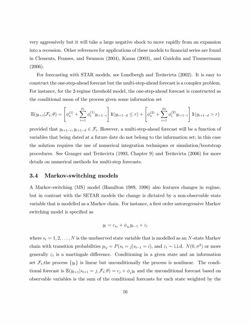
For forecasting with STAR models, see Lundbergh and Teräsvirta (2002). It is easy to

construct the one-step-ahead forecast but the multi-step-ahead forecast is a complex problem.

For instance, for the 2-regime threshold model, the one-step-ahead forecast is constructed as

the conditional mean of the process given some information set

E(yt+1jFt; �) ="�(1)o +

p1Xi=1

�(1)i yt+1�i

#1(yt+1�d � r) +

"�(2)o +

p2Xi=1

�(2)i yt+1�i

#1(yt+1�d > r)

provided that yt+1�i; yt+1�d 2 Ft: However, a multi-step-ahead forecast will be a function ofvariables that being dated at a future date do not belong to the information set; in this case

the solution requires the use of numerical integration techniques or simulation/bootstrap

procedures. See Granger and Teräsvirta (1993, Chapter 9) and Teräsvirta (2006) for more

details on numerical methods for multi-step forecasts.

3.4 Markov-switching models

A Markov-switching (MS) model (Hamilton 1989, 1996) also features changes in regime,

but in contrast with the SETAR models the change is dictated by a non-observable state

variable that is modelled as a Markov chain. For instance, a �rst order autoregressive Markov

switching model is speci�ed as

yt = cst + �styt�1 + "t

where st = 1; 2; : : : ; N is the unobserved state variable that is modelled as anN -state Markov

chain with transition probabilities pij = P (st = jjst�1 = i); and "t � i.i.d. N(0; �2) or moregenerally "t is a martingale di¤erence. Conditioning in a given state and an information

set Ft;the process fytg is linear but unconditionally the process is nonlinear. The condi-tional forecast is E(yt+1jst+1 = j;Ft; �) = cj + �jyt and the unconditional forecast based on

observable variables is the sum of the conditional forecasts for each state weighted by the

16

probability of being in that state,

E(yt+1jFt; �) =NXj=1

P (st+1 = jjFt; �)E(yt+1jst+1 = j;Ft; �):

The parameter vector � = (c1 : : : cN ; �1 : : : �N ; �2)0 as well as the transition probabilities pij

can be estimated by maximum likelihood.

MS models have been applying to the modeling of foreign exchange rates with mixed

success. Engel and Hamilton (1990) �t a two-state MS for the Dollar and �nd that there

are long swings and by that they reject the random walk behavior in the exchange rate.

Marsh (2000) estimates a two-state MS for the Deutschemark, the Pound Sterling, and the

Japanese Yen. Though the model approximates the characteristics of the data well, the

forecasting performance is poor when measured by the pro�t/losses generated by a set of

trading rules based on the predictions of the MS model. On the contrary, Dueker and Neely

(2007) �nd that for the same exchange rate a MS model with three states variables � in

the scale factor of the variance of a Student-t error, in the kurtosis of the error, and in the

expected return�produces out-of-sample excess returns that are slightly superior to those

generated by common trading rules. For stock returns, there is evidence that MS models

perform relatively well on describing two states in the mean (high/low returns) and two states

in the variance (stable/volatile periods) of returns (Maheu and McCurdy, 2000). In addition,

Perez-Quiros and Timmermann (2001) propose that the error term should be modelled as

a mixture of Gaussian and Student-t distributions to capture the outliers commonly found

in stock returns. This model provides some gains in predictive accuracy mainly for small

�rms returns. For interest rates in USA, Germany, and United Kingdom, Ang and Bekaert

(2002) �nd that a two-state MS model that incorporates information on international short

rate and on term spread is able to predict better than an univariate MS model. Additionally

they �nd that in USA the classi�cation of regimes correlates well with the business cycles.

SETAR, STAR, and MS models are successful speci�cations to approximate the charac-

teristics of �nancial and macroeconomic data. However, good in-sample performance does

not imply necessarily a good out-of-sample performance, mainly when compared to simple

linear ARMA models. The success of nonlinear models depends on how prominent the non-

17

linearity is in the data. We should not expect a nonlinear model to perform better than

a linear model when the contribution of the nonlinearity to the overall speci�cation of the

model is very small. As it is argued in Granger and Teräsvirta (1993), the prediction errors

generated by a nonlinear model will be smaller only when the nonlinear feature modelled

in-sample is also present in the forecasting sample.

3.5 A state dependent mixture model based on cross-sectionalranks

In the previous section, we have dealt with nonlinear time series models that only incorporate

time series information. González-Rivera, Lee, and Mishra (2008) propose a nonlinear model

that combines time series with cross sectional information. They propose the modelling of

expected returns based on the joint dynamics of a sharp jump in the cross-sectional rank

and the realized returns. They analyze the marginal probability distribution of a jump in

the cross-sectional rank within the context of a duration model, and the probability of the

asset return conditional on a jump specifying di¤erent dynamics depending on whether or

not a jump has taken place. The resulting model for expected returns is a mixture of normal

distributions weighted by the probability of jumping.

Let yi;t be the return of �rm i at time t; and fyi;tgMi=1 be the collection of asset returnsof the M �rms that constitute the market at time t: For each time t, the asset returns are

ordered from the smallest to the largest, and de�ne zi;t, the Varying Cross-sectional Rank

(VCR) of �rm i within the market, as the proportion of �rms that have a return less than

or equal to the return of �rm i. We write

zi;t �M�1MXj=1

1(yj;t � yi;t); (1)

where 1(�) is the indicator function, and for M large, zi;t 2 (0; 1]: Since the rank is a highlydependent variable, it is assumed that small movements in the asset ranking will not contain

signi�cant information and that most likely large movements in ranking will be the result of

news in the overall market and/or of news concerning a particular asset. Focusing on large

rank movements, we de�ne, at time t; a sharp jump as a binary variable that takes the value

18

one when there is a minimum (upward or downward) movement of 0.5 in the ranking of asset

i , and zero otherwise:

Ji;t � 1( jzi;t � zi;t�1j � 0:5): (2)

A jump of this magnitude brings the asset return above or below the median of the cross-

sectional distribution of returns. Note that this notion of jumps di¤ers from the more

traditional meaning of the word in the context of continuous-time modelling of the univariate

return process. A jump in the cross-sectional rank implicitly depends on numerous univariate

return processes.

The analytical problem now consists in modeling the joint distribution of the return yi;t

and the jump Ji;t, i.e. f(yi;t; Ji;tjFt�1) where Ft�1 is the information set up to time t�1: Sincef(yi;t; Ji;tjFt�1) = f1(Ji;tjFt�1)f2(yi;tjJi;t;Ft�1), the analysis focuses �rst on the modelling ofthe marginal distribution of the jump, and subsequently on the modelling of the conditional

distribution of the return.

Since Ji;t is a Bernoulli variable, the marginal distribution of the jump is f1(Ji;tjFt�1) =pJi;ti;t (1� pi;t)

(1�Ji;t) where pi;t � Pr(Ji;t = 1jFt�1) is the conditional probability of a jump inthe cross-sectional ranks. The modelling of pi;t is performed within the context of a dynamic

duration model speci�ed in calendar time as in Hamilton and Jordà (2002). The calendar

time approach is necessary because asset returns are reported in calendar time (days, weeks,

etc.) and it has the advantage of incorporating any other available information also reported

in calendar time.

It is easy to see that the probability of jumping and duration must have an inverse

relationship. If the probability of jumping is high, the expected duration must be short, and

viceversa. Let N(t) be the expected duration. The expected duration until the next jump in

the cross-sectional rank is given by N(t) =P1

j=1 j(1� pt)j�1pt = p�1t : Note that

P1j=0(1�

pt)j = p�1t : Di¤erentiating with respect to pt yields

P1j=0�j(1� pt)j�1 = �p�2t : Multiplying

by �pt givesP1

j=0 j(1 � pt)j�1pt = p�1t and thus

P1j=1 j(1 � pt)

j�1pt = p�1t : Consequently,

to model pi;t, it su¢ ces to model the expected duration and compute its inverse. Following

Hamilton and Jordà (2002), an autoregressive conditional hazard (ACH) model is speci�ed.

The ACH model is a calendar-time version of the autoregressive conditional duration (ACD)

19

of Engle and Russell (1998). In both ACD and ACH models, the expected duration is a

linear function of lag durations. However as the ACD model is set up in event time, there

are some di¢ culties on how to introduce information that arrives between events. This is

not the case in the ACH model because the set-up is in calendar time. In the ACD model,

the forecasting object is the expected time between events; in the ACH model, the objective

is to forecast the probability that the event will happen tomorrow given the information

known up to today. A general ACH model is speci�ed as

N(t) =

mXj=1

�jDN(t)�j +

rXj=1

�jN(t)�j: (3)

Since pt is a probability, it must be bounded between zero and one. This implies that the

conditional duration must have a lower bound of one. Furthermore, working in calendar

time it is possible to incorporate information that becomes available between jumps and can

a¤ect the probability of a jump in future periods. The conditional hazard rate is speci�ed

as

pt = [N(t�1) + �0Xt�1]

�1; (4)

whereXt�1 is a vector of relevant calendar time variables such as past VCRs and past returns.

This completes the marginal distribution of the jump f1(Ji;tjFt�1) = pJi;ti;t (1� pi;t)

(1�Ji;t):

On modelling f2(ytjJt;Ft�1; �2); it is assumed that the return to asset i may behave dif-ferently depending upon the occurrence of a jump. The modelling of two potential di¤erent

states (whether a jump has occurred or not) will permit to di¤erentiate whether the condi-

tional expected return is driven by active or/and passive movements in the asset ranking in

conjunction with its own return dynamics. A priori, di¤erent dynamics are possible in these

two states. A general speci�cation is

f2(ytjJt;Ft�1; �2) =�N(�1;t; �

21;t) if Jt = 1

N(�0;t; �20;t) if Jt = 0;

(5)

where �j;t is the conditional mean and �2j;t the conditional variance in each state (j = 1; 0).

Whether these two states are present in the data is an empirical question and it should be

answered through statistical testing.

20

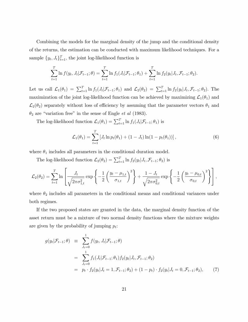
Combining the models for the marginal density of the jump and the conditional density

of the returns, the estimation can be conducted with maximum likelihood techniques. For a

sample fyt; JtgTt=1; the joint log-likelihood function is

TXt=1

ln f(yt; JtjFt�1; �) =TXt=1

ln f1(JtjFt�1; �1) +TXt=1

ln f2(ytjJt;Ft�1; �2):

Let us call L1(�1) =PT

t=1 ln f1(JtjFt�1; �1) and L2(�2) =PT

t=1 ln f2(ytjJt;Ft�1; �2): Themaximization of the joint log-likelihood function can be achieved by maximizing L1(�1) andL2(�2) separately without loss of e¢ ciency by assuming that the parameter vectors �1 and�2 are �variation free�in the sense of Engle et al (1983).

The log-likelihood function L1(�1) =PT

t=1 ln f1(JtjFt�1; �1) is

L1(�1) =TXt=1

[Jt ln pt(�1) + (1� Jt) ln(1� pt(�1))] ; (6)

where �1 includes all parameters in the conditional duration model.

The log-likelihood function L2(�2) =PT

t=1 ln f2(ytjJt;Ft�1; �2) is

L2(�2) =TXt=1

ln

24 Jtq2��21;t

exp

(�12

�yt � �1;t�1;t

�2)+

1� Jtq2��20;t

exp

(�12

�yt � �0;t�0;t

�2)35 ;where �2 includes all parameters in the conditional means and conditional variances under

both regimes.

If the two proposed states are granted in the data, the marginal density function of the

asset return must be a mixture of two normal density functions where the mixture weights

are given by the probability of jumping pt:

g(ytjFt�1; �) �1X

Jt=0

f(yt; JtjFt�1; �)

=1X

Jt=0

f1(JtjFt�1; �1)f2(ytjJt;Ft�1; �2)

= pt � f2(ytjJt = 1;Ft�1; �2) + (1� pt) � f2(ytjJt = 0;Ft�1; �2); (7)

21

as f1(JtjFt�1; �1) = pJtt (1� pt)(1�Jt): Therefore, the one-step ahead forecast of the return is

E(yt+1jFt; �) =Zyt+1�g(yt+1jFt; �)dyt+1 = pt+1(�1)��1;t+1(�2)+(1�pt+1(�1))��0;t+1(�2): (8)

The expected return is a function of the probability of jumping pt, which is a nonlinear

function of the information set as shown in (4). Hence the expected returns are nonlinear

functions of the information set, even in a simple case where �1;t and �0;t are linear.

This model was estimated for the returns of the constituents of the SP500 index from

1990 to 2000, and its performance was assessed in an out-of-sample exercise from 2001 to

2005 within the context of several trading strategies. Based on the one-step-ahead forecast of

the mixture model, a proposed trading strategy called VCR-Mixture Trading Rule is shown

to be a superior rule because of its ability to generate large risk-adjusted mean returns when

compared to other technical and model-based trading rules. The VCR-Mixture Trading Rule

is implemented by computing for each �rm in the SP500 index the one-step ahead forecast

of the return as in (8). Based on the forecasted returns fyi;t+1(�t)gT�1t=R , the investor predicts

the VCR of all assets in relation to the overall market, that is,

zi;t+1 =M�1MXj=1

1(yj;t+1 � yi;t+1); t = R; : : : ; T � 1; (9)

and buys the top K performing assets if their forecasted return is above the risk-free rate. In

every subsequent out-of-sample period (t = R; : : : ; T � 1), the investor revises her portfolio,selling the assets that fall out of the top performers and buying the ones that rise to the top,

and she computes the one-period portfolio return

�t+1 = K�1MXj=1

yj;t+1 � 1(zj;t+1 � zKt+1); t = R; : : : ; T � 1; (10)

where zKt+1 is the cuto¤ cross-sectional rank to select the K best performing stocks such thatPMj=1 1(zj;t+1 � zKt+1) = K. In the analysis of González-Rivera, Lee, and Mishra (2008) a

portfolio is formed with the top 1% (K = 5 stocks) performers in the SP500 index. Every

asset in the portfolio is weighted equally. The evaluation criterion is to compute the �mean

trading return�over the forecasting period

MTR = P�1T�1Xt=R

�t+1:

22

It is also possible to correct MTR according to the level of risk of the chosen portfolio. For

instance, the traditional Sharpe ratio will provide the excess return per unit of risk measured

by the standard deviation of the selected portfolio

SR = P�1T�1Xt=R

(�t+1 � rf;t+1)

��t+1(�t);

where rf;t+1 is the risk free rate. The VCR-Mixture Trading Rule produces a weekly MTR

of 0:243% (63:295% cumulative return over 260 weeks), equivalent to a yearly compounded

return of 13:45%; that is signi�cantly more than the next most favorable rule, which is the

Buy-and-Hold-the-Market Trading Rule with a weekly mean return of �0:019%, equivalentto a yearly return of �1:00%. To assess the return-risk trade o¤, we implement the Sharperatio. The largest SR (mean return per unit of standard deviation) is provided by the VCR-

Mixture rule with a weekly return of 0:151% (8:11% yearly compounded return per unit of

standard deviation), which is lower than the mean return provided by the same rule under

theMTR criterion, but still a dominant return when compared to the mean returns provided

by the Buy-and-Hold-the-Market Trading Rule.

3.6 Random �elds

Hamilton (2001) proposed a �exible parametric regression model where the conditional mean

has a linear parametric component and a potential nonlinear component represented by an

isotropic Gaussian random �eld. The model has a nonparametric �avor because no functional

form is assumed but, nevertheless, the estimation is fully parametric.

A scalar random �eld is de�ned as a function m(!; x) : �A! R such that m(!; x) is

a random variable for each x 2 A where A � Rk: A random �eld is also denoted as m(x).

If m(x) is a system of random variables with �nite dimensional Gaussian distributions,

then the scalar random �eld is said to be Gaussian and it is completely determined by its

mean function �(x) = E [m(x)] and its covariance function with typical element C(x; z) =E [(m(x)� �(x))(m(z)� �(z))] for any x; z 2 A. The random �eld is said to be homogeneousor stationary if �(x) = � and the covariance function depends only on the di¤erence vector

x � z and we should write C(x; z) = C(x � z). Furthermore, the random �eld is said to

23

be isotropic if the covariance function depends on d(x; z), where d(�) is a scalar measure ofdistance. In this situation we write C(x; z) = C(d(x; z)).

The speci�cation suggested by Hamilton (2001) can be represented as

yt = �0 + x0t�1 + �m(g � xt) + �t; (11)

for yt 2 R and xt 2 Rk, both stationary and ergodic processes. The conditional mean has

a linear component given by �0 + x0t�1 and a nonlinear component given by �m(g � xt);

where m(z); for any choice of z; represents a realization of a Gaussian and homogenous

random �eld with a moving average representation; xt could be predetermined or exogenous

and is independent of m(�), and �t is a sequence of independent and identically distributedN(0; �2) variates independent of bothm(�) and xt as well as of lagged values of xt: The scalarparameter � represents the contribution of the nonlinear part to the conditional mean, the

vector g 2 Rk0;+ drives the curvature of the conditional mean, and the symbol � denotes

element-by-element multiplication.

Let Hk be the covariance (correlation) function of the random �eld m(�) with typicalelement de�ned as Hk(x; z) = E [m(x)m(z)]. Hamilton (2001) proved that the covariancefunction depends solely upon the Euclidean distance between x and z, rendering the random

�eld isotropic. For any x and z 2 Rk; the correlation between m(x) and m(z) is given by

the ratio of the volume of the overlap of k-dimensional unit spheroids centered at x and z

to the volume of a single k-dimensional unit spheroid. If the Euclidean distance between x

and z is greater than two, the correlation between m(x) and m(z) will be equal to zero. The

general expression of the correlation function is

Hk(h) =

�Gk�1(h; 1)=Gk�1(0; 1)

0if h � 1if h > 1

; (12)

Gk(h; r) =

Z r

h

(r2 � w2)k=2dw;

where h � 12dL2(x; z); and dL2(x; z) � [(x� z)0(x� z)]1=2 is the Euclidean distance between

x and z.

Within the speci�cation (11), Dahl and González-Rivera (2003a) provided alternative

representations of the random �eld that permit the construction of Lagrange multiplier tests

24

for neglected nonlinearity, which circumvent the problem of unidenti�ed nuisance parameters

under the null of linearity and, at the same time, they are robust to the speci�cation of the

covariance function associated with the random�eld. They modi�ed the Hamilton framework

in two directions. First, the random �eld is speci�ed in the L1 norm instead of the L2 norm,

and secondly they considered random �elds that may not have a simple moving average

representation. The advantage of the L1 norm, which is exploited in the testing problem,

is that this distance measure is a linear function of the nuisance parameters, in contrast to

the L2 norm which is a nonlinear function. Logically, Dahl and González-Rivera proceeded

in an opposite fashion to Hamilton. Whereas Hamilton �rst proposed a moving average

representation of the random �eld, and secondly, he derived its corresponding covariance

function, Dahl and González-Rivera �rst proposed a covariance function, and secondly they

inquire whether there is a random �eld associated with it. The proposed covariance function

is

Ck(h�) =

�(1� h�)2k

0if h� � 1if h� > 1

; (13)

where h� � 12dL1(x; z) =

12jx � zj01: The function (13) is a permissible covariance, that

is, it satis�es the positive semide�niteness condition, which is q0Ckq � 0 for all q 6= 0T .

Furthermore, there is a random �eld associated with it according to the Khinchin�s theorem

(1934) and Bochner�s theorem (1959). The basic argument is that the class of functions

which are covariance functions of homogenous random �elds coincides with the class of

positive semide�nite functions. Hence, (13) being a positive semide�nite function must be

the covariance function of a homogenous random �eld.

The estimation of these models is carried out by maximum likelihood. From model (11),

we can write y � N(X�; �2Ck + �2IT ) where y = (y1; y2; :::; yT )0, X1 = (x01; x

02; :::; x

0T )0,

X = (1 : X1), � = (�0; �01)0, � = (�1; �2; :::; �T )

0and �2 is the variance of �t. Ck is a generic

covariance function associated with the random �eld, which could be equal to the Hamilton

spherical covariance function in (12), or to the covariance in (13). The log-likelihood function

25

corresponding to this model is

`(�; �2; g; �2) = �T2log(2�)� 1

2log j�2Ck + �2IT j (14)

�12(y �X�)0(�2Ck + �2IT )

�1(y �X�):

The �exible regression model has been applied successfully to detect nonlinearity in the

quarterly growth rate of the US real GNP (Dahl and González-Rivera 2003b) and in the

Industrial Production Index of sixteen OECD countries (Dahl and González-Rivera 2003a).

This technology is able to mimic the characteristics of the actual US business cycle. The cycle

is dissected according to measures of duration, amplitude, cumulation and excess cumulation

of the contraction and expansion phases. In contrast to Harding and Pagan (2002) who �nd

that nonlinear models are not uniformly superior to linear ones, the �exible regression model

represents a clear improvement over linear models, and it seems to capture just the right

shape of the expansion phase as opposed to Hamilton (1989) and Durland and McCurdy

(1994) models, which tend to overestimate the cumulation measure in the expansion phase.

It is found that the expansion phase must have at least two subphases: an aggressive early

expansion after the trough, and a moderate/slow late expansion before the peak implying the

existence of an in�exion point that we date approximately around one-third into the duration

of the expansion phase. This shape lends support to parametric models of the growth rate

that allow for three regimes (Sichel, 1994), as opposed to models with just two regimes

(contractions and expansions). For the Industrial Production Index, testing for nonlinearity

within the �exible regression framework brings similar conclusions to those in Teräsvirta

and Anderson (1992), who propose parametric STAR models for industrial production data.

However, the tests proposed in Dahl and González-Rivera (2003a), which have superior

performance to detect smooth transition dynamics, seem to indicate that linearity cannot

be rejected in the industrial production indexes of Japan, Austria, Belgium and Sweden as

opposed to the �ndings of Teräsvirta and Anderson.

3.7 Nonlinear factor models

For the last ten years forecasting using a data-rich environment has been one of the most

researched topic in economics and �nance, see Stock and Watson (2002, 2006). In this

26

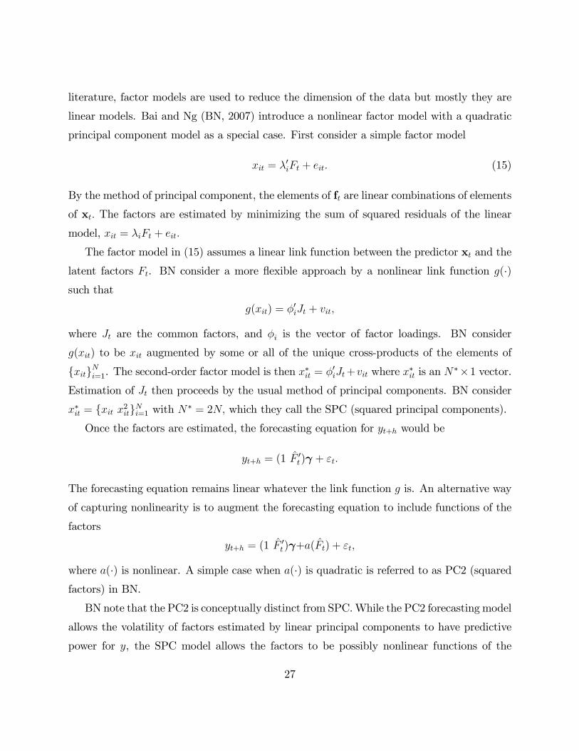
literature, factor models are used to reduce the dimension of the data but mostly they are

linear models. Bai and Ng (BN, 2007) introduce a nonlinear factor model with a quadratic

principal component model as a special case. First consider a simple factor model

xit = �0iFt + eit: (15)

By the method of principal component, the elements of ft are linear combinations of elements

of xt: The factors are estimated by minimizing the sum of squared residuals of the linear

model, xit = �iFt + eit:

The factor model in (15) assumes a linear link function between the predictor xt and the

latent factors Ft. BN consider a more �exible approach by a nonlinear link function g(�)such that

g(xit) = �0iJt + vit;

where Jt are the common factors, and �i is the vector of factor loadings. BN consider

g(xit) to be xit augmented by some or all of the unique cross-products of the elements of

fxitgNi=1. The second-order factor model is then x�it = �0iJt+vit where x�it is an N

��1 vector.Estimation of Jt then proceeds by the usual method of principal components. BN consider

x�it = fxit x2itgNi=1 with N� = 2N; which they call the SPC (squared principal components).

Once the factors are estimated, the forecasting equation for yt+h would be

yt+h = (1 F0t) + "t:

The forecasting equation remains linear whatever the link function g is. An alternative way

of capturing nonlinearity is to augment the forecasting equation to include functions of the

factors

yt+h = (1 F0t) +a(Ft) + "t;

where a(�) is nonlinear. A simple case when a(�) is quadratic is referred to as PC2 (squaredfactors) in BN.

BN note that the PC2 is conceptually distinct from SPC.While the PC2 forecasting model

allows the volatility of factors estimated by linear principal components to have predictive

power for y, the SPC model allows the factors to be possibly nonlinear functions of the

27

predictors while maintaining a linear relation between the factors and y. Ludvigson and Ng

(2005) found that the square of the �rst factor estimated from a set of �nancial factors (i.e.,

volatility of the �rst factor) is signi�cant in the regression model for the mean excess returns.

In contrast, factors estimated from the second moment of data (i.e., volatility factors) are

much weaker predictors of excess returns.

3.8 Arti�cial neural network models

Consider an augmented single hidden layer feedforward neural network model f(xt; �) in

which the network output yt is determined given input xt as

yt = f(xt; �) + "t

= xt� +

qXj=1

�j (xt j) + "t

where � = (�0 0 �0)0; � is a conformable column vector of connection strength from the input

layer to the output layer; j is a conformable column vector of connection strength from the

input layer to the hidden units, j = 1; : : : ; q; �j is a (scalar) connection strength from the

hidden unit j to the output unit, j = 1; : : : ; q; and is a squashing function (e.g., the logistic

squasher) or a radial basis function. Input units x send signals to intermediate hidden units,

then each of hidden unit produces an activation that then sends signals toward the output

unit. The integer q denotes the number of hidden units added to the a¢ ne (linear) network.

When q = 0, we have a two layer a¢ ne network yt = xt� + "t: Hornick, Stinchcombe and

White (1989) show that neural network is a nonlinear �exible functional form being capable

of approximating any Borel measurable function to any desired level of accuracy provided

su¢ ciently many hidden units are available. Stinchcombe and White (1998) show that this

result holds for any (�) belonging to the class of �generically comprehensively revealing�functions. These functions are �comprehensively revealing�in the sense that they can reveal

arbitrary model misspeci�cations E(ytjxt) 6= f(xt; ��) with non-zero probability and they are

�generic�in the sense that almost any choice for will reveal the misspeci�cation.

We build an arti�cial neural network (ANN) model based on a test for neglected non-

linearity likely to have power against a range of alternatives . See White (1989) and Lee,

28

White, and Granger (1993) on the neural network test and its comparison with other spec-

i�cation tests. The neural network test is based on a test function h(xt) chosen as the

activations of �phantom�hidden units (xt�j); j = 1; : : : ; q; where �j are random column

vectors independent of xt. That is,

E[ (xt�j)"�t j�j] = E[ (xt�j)"�t ] = 0 j = 1; : : : ; q; (16)

under H0, so that

E(t"�t ) = 0; (17)

where t = ( (xt�1); : : : ; (xt�q))0 is a phantom hidden unit activation vector. Evidence

of correlation of "�t with t is evidence against the null hypothesis that yt is linear in mean.

If correlation exists, augmenting the linear network by including an additional hidden unit

with activations (xt�j) would permit an improvement in network performance. Thus the

tests are based on sample correlation of a¢ ne network errors with phantom hidden unit

activations,

n�1nXt=1

t"t = n�1nXt=1

t(yt � xt�): (18)

Under suitable regularity conditions it follows from the central limit theorem that n�1=2Pn

t=1t"td! N(0;W �) as n!1, and if one has a consistent estimator for its asymptotic covariancematrix, say Wn, then an asymptotic chi-square statistic can be formed as

(n�1=2nXt=1

t"t)0W�1

n (n�1=2nXt=1

t"t)d! �2(q): (19)

Elements of t tend to be collinear with Xt and with themselves. Thus LWG conduct a

test on q� < q principal components of t not collinear with xt; denoted �t : This test is to

determine whether or not there exists some advantage to be gained by adding hidden units

to the a¢ ne network. We can estimate Wn robust to the conditional heteroskedasticity, or

we may use with the empirical null distribution of the statistic computed by a bootstrap

procedure that is robust to the conditional heteroskedasticity, e.g., wild bootstrap.

Estimation of an ANN model may be tedious and sometimes results in unreliable es-

timates. Recently, White (2006) proposes a simple algorithm called QuickNet, a form of

29

�relaxed greedy algorithm�because QuickNet searches for a single best additional hidden

unit based on a sequence of OLS regressions, that may be analogous to the least angular

regressions (LARS) of Efron, Hastie, Johnstone, and Tibshirani (2004). The simplicity of

the QuickNet algorithm achieves the bene�ts of using a forecasting model that is nonlinear

in the predictors while mitigating the other computational challenges to the use of nonlinear

forecasting methods. See White (2006, Section 5) for more details on QuickNet, and for

other issues of controlling for over�t and the selection of the random parameter vectors �j

independent of xt.

Campbell, Lo, and MacKinlay (1997, Section 12.4) provide a review of these models.

White (2006) reviews the research frontier in ANN models. Trippi and Turban (1992) review

the applications of ANNs to �nance and investment.

3.9 Functional coe¢ cient models

A functional coe¢ cient model is introduced by Cai, Fan, and Yao (CFY, 2000), with time-

varying and state-dependent coe¢ cients. It can be viewed as a special case of Priestley�s

(1980) state-dependent model, but it includes the models of Tong (1990), Chen and Tsay

(1993) and regime-switching models as special cases. Let f(yt; st)0gnt=1 be a stationary process,where yt and st are scalar variables. Also let Xt � (1; yt�1; : : : ; yt�d)0. We assume

E(ytjFt�1) = a0(st) +dXj=1

aj(st)yt�j;

where the faj(st)g are the autoregressive coe¢ cients depending on st; which may be chosenas a function of Xt or something else. Intuitively, the functional coe¢ cient model is an

AR process with time-varying autoregressive coe¢ cients. The coe¢ cient functions faj(st)gcan be estimated by local linear regression. At each point s, we approximate aj(st) locally

by a linear function aj(st) � aj + bj(st � s); j = 0; 1; :::; d; for st near s; where aj and

bj are constants. The local linear estimator at point s is then given by aj(s) = aj; where

f(aj; bj)gdj=0 minimizes the sum of local weighted squaresPn

t=1[yt � E(ytjFt�1)]2Kh(st � s);

with Kh(�) � K(�=h)=h for a given kernel function K(�) and bandwidth h � hn ! 0 as

n!1: CFY (2000, p. 944) suggest to select h using a modi�ed multi-fold �leave-one-out-

30

type�cross-validation based on MSFE.

It is important to choose an appropriate smooth variable st. Knowledge on data or

economic theory may be helpful. When no prior information is available, st may be chosen

as a function of explanatory vector Xt or using such data-driven methods as AIC and cross-

validation. See Fan, Yao and Cai (2003) for further discussion on the choice of st: For

exchange rate changes, Hong and Lee (2003) choose st as the di¤erence between the exchange

rate at time t� 1 and the moving average of the most recent L periods of exchange rates attime t� 1. The moving average is a proxy for the local trend at time t� 1. Intuitively, thischoice of st is expected to reveal useful information on the direction of changes.

To justify the use of the functional coe¢ cient model, CFY (2000) suggest a goodness-of-

�t test for an AR(d) model against a functional coe¢ cient model. The null hypothesis of

AR(d) can be stated as

H0 : aj(st) = �j; j = 0; 1; : : : d;

where �j is the autoregressive coe¢ cient in AR(d). Under H0; fytg is linear in mean con-ditional on Xt. Under the alternative to H0, the autoregressive coe¢ cients depend on stand the AR(d) model su¤ers from �neglected nonlinearity�. To test H0, CFY compares theresidual sum of squares (RSS) under H0

RSS0 �nXt=1

"2t =nXt=1

[Yt � �0 �dXj=1

�jYt�j]2

with the RSS under the alternative

RSS1 �nXt=1

~"2t =nXt=1

[Yt � a0(st)�dXj=1

aj(st)Yt�j]2:

The test statistic is Tn = (RSS0 � RSS1)=RSS1. We reject H0 for large values of Tn.CFY suggest the following bootstrap method to obtain the p-value of Tn: (i) generate the

bootstrap residuals f"btgnt=1 from the centered residuals ~"t��" where �" � n�1Pn

t=1 ~"t and de�ne

ybt � X 0t�+"

bt ; where � is the OLS estimator for AR(d); (ii) calculate the bootstrap statistic T

bn

using the bootstrap sample fybt ; X 0t; stgnt=1; (iii) repeat steps (i) and (ii) B times (b = 1; :::; B)

and approximate the bootstrap p-value of Tn by B�1PBb=1 1(T

bn � Tn): See Hong and Lee

31

(2003) for empirical application of the functional coe¢ cient model to forecasting foreign

exchange rates.

3.10 Nonparametric regression

Let fyt; xtg; t = 1; : : : ; n; be stochastic processes, where yt is a scalar and xt = (xt1; : : : ; xtk)is a 1� k vector which may contain the lagged values of yt. Consider the regression model

yt = m(xt) + ut

where m(xt) = E (ytjxt) is the true but unknown regression function and ut is the error termsuch that E(utjxt) = 0:If m(xt) = g(xt; �) is a correctly speci�ed family of parametric regression functions then

yt = g(xt; �) + ut is a correct model and, in this case, one can construct a consistent least

squares (LS) estimator ofm(xt) given by g(xt; �); where � is the LS estimator of the parameter

�:

In general, if the parametric regression g(xt; �) is incorrect or the form of m(xt) is un-

known then g(xt; �) may not be a consistent estimator of m(xt): For this case, an alternative

approach to estimate the unknown m(xt) is to use the consistent nonparametric kernel re-

gression estimator which is essentially a local constant LS (LCLS) estimator. To obtain this

estimator take a Taylor series expansion of m(xt) around x so that

yt = m(xt) + ut

= m(x) + et

where et = (xt � x)m(1)(x) + 12(xt � x)2m(2)(x) + � � � + ut and m(s)(x) represents the s-th

derivative of m(x) at xt = x: The LCLS estimator can then be derived by minimizing

nXt=1

e2tKtx =

nXt=1

(yt �m(x))2Ktx

with respect to constantm(x); where Ktx = K�xt�xh

�is a decreasing function of the distances

of the regressor vector xt from the point x = (x1; : : : ; xk); and h ! 0 as n ! 1 is the

32

window width (smoothing parameter) which determines how rapidly the weights decrease as

the distance of xt from x increases. The LCLS estimator so estimated is

m(x) =

Pnt=1 ytKtxPnt=1Ktx

= (i0K(x)i)�1i0K(x)y

whereK(x) is the n�n diagonal matrix with the diagonal elementsKtx (t = 1; : : : ; n); i is an

n�1 column vector of unit elements, and y is an n�1 vector with elements yt (t = 1; : : : ; n).The estimator m(x) is due to Nadaraya (1964) and Watson (1964) (NW) who derived this

in an alternative way. Generally m(x) is calculated at the data points xt; in which case we

can write the leave-one out estimator as

m(x) =

Pnt0=1;t0 6=t yt0Kt0tPnt0=1;t0 6=tKt0t

;

where Kt0t = K�xt0�xt

h

�: The assumption that h ! 0 as n ! 1 gives xt � x = O(h) ! 0

and hence Eet ! 0 as n ! 1: Thus the estimator m(x) will be consistent under certain

smoothing conditions on h;K; and m(x): In small samples however Eet 6= 0 so m(x) will bea biased estimator, see Pagan and Ullah (1999) for details on asymptotic and small sample

properties.

An estimator which has a better small sample bias and hence the mean square error

(MSE) behavior is the local linear LS (LLLS) estimator. In the LLLS estimator we take a

�rst order Taylor-Series expansion of m(xt) around x so that

yt = m(xt) + ut = m(x) + (xt � x)m(1)(x) + vt

= �(x) + xt�(x) + vt

= Xt�(x) + vt

where Xt = (1 xt) and �(x) = [�(x) �(x)0]0 with �(x) = m(x) � x�(x) and �(x) = m(1)(x):

The LLLS estimator of �(x) is then obtained by minimizing

nXt=1

v2tKtx =

nXt=1

(yt �Xt�(x))2Ktx

sand it is given by~�(x) = (X0K(x)X)�1X0K(x)y: (20)

33

where X is an n� (k + 1) matrix with the tth row Xt (t = 1; : : : ; n):

The LLLS estimator of �(x) and �(x) can be calculated as ~�(x) = (1 0)~�(x) and ~�(x) =

(0 1)~�(x): This gives

~m(x) = (1 x)~�(x) = ~�(x) + x~�(x):

Obviously when X = i; ~�(x) reduces to the NW�s LCLS estimator m(x): An extension of

the LLLS is the local polynomial LS (LPLS) estimators, see Fan and Gijbels (1996).

In fact one can obtain the local estimators of a general nonlinear model g(xt; �) by

minimizingnXt=1

[yt � g(xt; �(x))]2Ktx

with respect to �(x): For g(xt; �(x)) = Xt�(x) we get the LLLS in (20). Further when

h = 1; Ktx = K(0) is a constant so that the minimization of K(0)P[yt � g(xt; �(x))]

2 is

the same as the minimization ofP[yt � g(xt; �)]

2, that is the local LS becomes the global

LS estimator �.

The LLLS estimator in (20) can also be interpreted as the estimator of the functional

coe¢ cient (varying coe¢ cient) linear regression model

yt = m(xt) + ut

= Xt�(xt) + ut

where �(xt) is approximated locally by a constant �(xt) ' �(x): The minimization ofPu2tKtx

with respect to �(x) then gives the LLLS estimator in (20), which can be interpreted as the

LC varying coe¢ cient estimator. An extension of this is to consider the linear approximation

�(xt) ' �(x) +D(x)(xt � x)0 where D(x) = @�(xt)@x0t

evaluated at xt = x: In this case

yt = m(xt) + ut = Xt�(xt) + ut

' Xt�(x) +XtD(x)(xt � x)0 + ut

= Xt�(x) + [(xt � x)Xt]vecD(x) + ut

= Xxt �x(x) + ut

where Xxt = [Xt (xt � x)Xt] and �

x(x) = [�(x)0 (vecD(x))0]0. The LL varying coe¢ cient

34

estimator of �x(x) can then be obtained by minimizing

nXt=1

[yt �Xxt �x(x)]2Ktx

with respect to �x(x) as_�x(x) = (Xx0K(x)Xx)�1Xx0K(x)y: (21)

From this _�(x) = (I 0)_�x(x); and hence

_m(x) = (1 x 0)_�x(x) = (1 x) _�(x):

The above idea can be extended to the situations where �t = (xt zt) such that

E(ytj�t) = m(�t) = m(xt; zt) = Xt�(zt);

where the coe¢ cients are varying with respect to only a subset of �t; zt is 1 � l and �t is

1 � p; p = k + l: Examples of these include functional coe¢ cient autoregressive models of

Chen and Tsay (1993) and CFY (2000), random coe¢ cient models of Raj and Ullah (1981),

smooth transition autoregressive models of Granger and Teräsvirta (1993), and threshold

autoregressive models of Tong (1990).

To estimate �(zt) we can again do a local constant approximation �(zt) ' �(z) and then

minimizeP[yt �Xt�(z)]

2Ktz with respect to �(z); where Ktz = K( zt�zh): This gives the LC

varying coe¢ cient estimator

~�(z) = (X0K(z)X)�1X0K(z)y (22)

where K(z) is a diagonal matrix of Ktz; t = 1; : : : ; n:When z = x; (22) reduces to the LLLS

estimator ~�(x) in (20).

CFY (2000) consider a local linear approximation �(zt) ' �(z) +D(z)(zt � z)0: The LL

varying coe¢ cient estimator of CFY is then obtained by minimizing

nXt=1

[yt �Xt�(zt)]2Ktz =

nXt=1

[yt �Xt�(z)� [(zt � z)Xt]vecD(z)]2Ktz

=

nXt=1

[yt �Xzt �z(z)]2Ktz

35

with respect to �z(z) = [�(z)0 (vecD(z))0]0 where Xzt = [Xt (zt � z)Xt]: This gives

��z(z) = (Xz0K(z)Xz)�1Xz0K(z)y; (23)

and ��(z) = (I 0)��z(z): Hence

�m(�) = (1 x 0)��z(z) = (1 x)��(z):

For the asymptotic properties of these varying coe¢ cient estimators, see CFY (2000). When

z = x; (23) reduces to the LL varying coe¢ cient estimator _�x(x) in (21). See Lee and Ullah

(2001) for more discussion of these models and issues of testing nonlinearity.

3.11 Regime switching autoregressive model between unit rootand stationary root

To avoid the usual dichotomy between unit-root nonstationarity and stationarity, we may

consider models that permit two regimes of unit root nonstationarity and stationarity.

One model is the Innovation Regime-Switching (IRS) model of Kuan, Huang, and Tsay

(2005). Intuitively, it may be implausible to believe that all random shocks exert only

one e¤ect (permanent or transitory) on future �nancial asset prices in a long time span.

This intuition underpins the models that allow for breaks, stochastic unit root, or regime

switching. As an alternative, Kuan, Huang, and Tsay (2005) propose the IRS model that

permits the random shock in each period to be permanent or transitory, depending on

a switching mechanism, and hence admits distinct dynamics (unit-root nonstationarity or

stationarity) in di¤erent periods. Under the IRS framework, standard unit-root models and

stationarity models are just two extreme cases. By applying the IRS model to real exchange

rate, they circumvent the di¢ culties arising from unit-root (or stationarity) testing. They

allow the data to speak for themselves, rather than putting them in the straitjacket of unit-

root nonstationarity or stationarity. Huang and Kuan (2007) re-examine long-run PPP based

on the IRS model and their empirical study on U.S./U.K. real exchange rates shows that

there are both temporary and permanent in�uences on the real exchange rate such that

approximately 42% of the shocks in the long run are more likely to have a permanent e¤ect.

They also found that transitory shocks dominate in the �xed-rate regimes, yet permanent

36

shocks play a more important role during the �oating regimes. Thus, the long-run PPP is

rejected due to the presence of a signi�cant amount of permanent shocks, but there are still

long periods of time in which the deviations from long-run PPP are only transitory.

Another model is a threshold unit root (TUR) model or threshold integrated moving

average (TIMA) model of Gonzalo and Martíneza (2006). Based on this model they examine

whether large and small shocks have di¤erent long-run e¤ects, as well as whether one of them

is purely transitory. They develop a new nonlinear permanent�transitory decomposition,

that is applied to US stock prices to analyze the quality of the stock market.

Comparison of these two models with the linear autoregressive model with a unit root or

a stationary AR model for the out-of-sample forecasting remains to be examined empirically.

3.12 Bagging nonlinear forecasts

To improve on unstable forecasts, bootstrap aggregating or bagging is introduced by Breiman

(1996a). Lee and Yang (2006) show how bagging works for binary and quantile predictions.

Lee and Yang (2006) attributed part of the success of the bagging predictors to the small

sample estimation uncertainties. Therefore, a question that may arise is that whether the

good performance of bagging predictors critically depends on algorithms we employ in non-

linear estimation.

They �nd that bagging improves the forecasting performance of predictors on highly

nonlinear regression models � e.g., arti�cial neural network models, especially when the

sample size is limited. It is usually hard to choose the number of hidden nodes and the

number of inputs (or lags), and to estimate the large number of parameters in an ANN

model. Therefore, a neural network model generate poor predictions in a small sample. In

such cases, bagging can do a valuable job to improve the forecasting performance as shown

in Lee and Yang (2006), con�rming the result of Breiman (1996b). A bagging predictor

is a combined predictor formed over a set of training sets to smooth out the �instability�

caused by parameter estimation uncertainty and model uncertainty. A predictor is said to

be �unstable� if a small change in the training set will lead to a signi�cant change in the

predictor (Breiman, 1996b).

37

As bagging would be valuable in nonlinear forecasting, in this section, we will show how

a bagging predictor may improve the predicting performance of its underlying predictor. Let

Dt � f(Ys;Xs�1)gts=t�R+1 (t = R; : : : ; T )

be a training set at time t and let '(Xt;Dt) be a forecast of Yt+1 or of the binary variableGt+1 � 1(Yt+1 � 0) using this training set Dt and the explanatory variable vector Xt. The

optimal forecast '(Xt;Dt) for Yt+1 will be the conditional mean of Yt+1 given Xt under the

squared error loss function, or the conditional quantile of Yt+1 on Xt if the loss is a tick

function. Below we also consider the binary forecast for Gt+1 � 1(Yt+1 � 0).Suppose each training set Dt consists of R observations generated from the underlying

probability distribution P. The forecast f'(Xt;Dt)gTt=R can be improved if more trainingsets were able to be generated from P and the forecast can be formed from averaging the

multiple forecasts obtained from the multiple training sets. Ideally, if P were known and

multiple training sets D(j)t (j = 1; : : : ; J) may be drawn from P, an ensemble aggregating

predictor 'A(Xt) can be constructed by the weighted averaging of '(Xt;D(j)t ) over j, i.e.,

'A(Xt) � EDt'(Xt;Dt) �JXj=1

wj;t'(Xt;D(j)t );

where EDt (�) denotes the expectation over P, wj;t is the weight function withPJ

j=1wj;t = 1,

and the subscript A in 'A denotes �aggregation�.

Lee and Yang (2006) show that the ensemble aggregating predictor 'A(Xt) has not a

larger expected loss than the original predictor '(Xt;Dt): For any convex loss function c(�)on the forecast error zt+1, we will have

EDt;Yt+1;Xtc(zt+1) � EYt+1;Xtc(EDt(zt+1));

where EDt(zt+1) is the aggregating forecast error, and EDt;Yt+1;Xt (�) � EXt [EYt+1jXtfEDt (�) jXtg]denotes the expectation EDt (�) taken over P (i.e., averaging over the multiple training setsgenerated from P), then taking an expectation of Yt+1 conditioning on Xt, and then taking

an expectation of Xt: Similarly we de�ne the notation EYt+1;Xt (�) � EXt [EYt+1jXt (�) jXt]:

38

Therefore, the aggregating predictor will always have no larger expected cost than the origi-

nal predictor for a convex loss function '(Xt; Dt). The examples of the convex loss function

includes the squared error loss and a tick (or check) loss ��(z) � [�� 1(z < 0)]z:How much this aggregating predictor can improve depends on the distance between

EDt;Yt+1;Xtc(zt+1) and EYt+1;Xtc(EDt(zt+1)). We can de�ne this distance by� � EDt;Yt+1;Xtc(zt+1)�EYt+1;Xtc(EDt(zt+1)). Therefore, the e¤ectiveness of the aggregating predictor depends on theconvexity of the cost function. The more convex is the cost function, the more e¤ective this

aggregating predictor can be. If the loss function is the squared error loss, then it can be

shown that � = VDt ['(Xt;Dt)] is the variance of the predictor, which measures the �in-stability�of the predictor. See Lee and Yang (2006, Proposition 1) and Breiman (1996b).

If the loss is the tick function, the e¤ectiveness of bagging is also di¤erent for di¤erent

quantile predictions: bagging works better for tail-quantile predictions than for mid-quantile

predictions.

In practice, however, P is not known. In that case we may estimate P by its empirical

distribution, P(Dt); for a given Dt. Then, from the empirical distribution P(Dt); multipletraining sets may be drawn by the bootstrap method. Bagging predictors, 'B(Xt;D�t );can then be computed by taking weighted average of the predictors trained over a set of

bootstrap training sets. More speci�cally, the bagging predictor 'B(Xt;D�t ) can be obtainedin the following steps:

1. Given a training set of data at time t; Dt � f(Ys;Xs�1)gts=t�R+1, construct the jthbootstrap sample D�(j)t � f(Y �(j)

s ;X�(j)s�1)gts=t�R+1, j = 1; : : : ; J; according to the empir-

ical distribution of P(Dt) of Dt:

2. Train the model (estimate parameters) from the jth bootstrapped sample D�(j)t .

3. Compute the bootstrap predictor '�(j)(Xt;D�(j)t ) from the jth bootstrapped sample

D�(j)t .

4. Finally, for mean and quantile forecast, the bagging predictor 'B(Xt;D�t ) can be con-

39

structed by averaging over J bootstrap predictors

'B(Xt;D�t ) �JXj=1

wj;t'�(j)(Xt;D�(j)t );

and for binary forecast, the bagging binary predictor 'B(Xt;D�t ) can be constructedby majority voting over J bootstrap predictors:

'B(Xt;D�t ) � 1

JXj=1

wj;t'�(j)(Xt;D�(j)t ) > 1=2

!

withPJ

j=1 wj;t = 1 in both cases.

One concern of applying bagging to time series is whether a bootstrap can provide a sound

simulation sample for dependent data, for which the bootstrap is required to be consistent. It

has been shown that some bootstrap procedure (such as moving block bootstrap) can provide

consistent densities for moment estimators and quantile estimators. See, e.g., Fitzenberger

(1997).

4 Nonlinear forecasting models for the conditional vari-ance

4.1 Nonlinear parametric models for volatility

Volatility models are of paramount importance in �nancial economics. Issues such as port-

folio allocation, option pricing, risk management, and generally any decision making under

uncertainty rely on the understanding and forecasting of volatility. This is one of the most

active ares of research in time series econometrics. Important surveys as in Bollerslev, Chou,

and Kroner (1992), Bera and Higgins (1993), Bollerslev, Engle, and Nelson (1994), Poon and

Granger (2003), and Bauwens, Laurent, and Rombouts (2006) attest to the variety of issues

in volatility research. The motivation for the introduction of the �rst generation of volatility

models namely the ARCH models of Engle (1982) was to account for clusters of activity and

fat-tail behavior of �nancial data. Subsequent models accounted for more complex issues.

Among others and without being exclusive, we should mention issues related to asymmetric

40

responses of volatility to news, probability distribution of the standardized innovations, i.i.d.

behavior of the standardized innovation, persistence of the volatility process, linkages with

continuous time models, intraday data and unevenly spaced observations, seasonality and

noise in intraday data. The consequence of this research agenda has been a vast array of

speci�cations for the volatility process.

Suppose that the return series fytgT+1t=1 of a �nancial asset follows the stochastic process

yt+1 = �t+1 + "t+1; where E(yt+1jFt) = �t+1(�) and E("2t+1jFt) = �2t+1(�) given the informa-

tion set Ft (�-�eld) at time t. Let zt+1 � "t+1=�t+1 have the conditional normal distribution

with zero conditional mean and unit conditional variance. Volatility models can be classi�ed

in three categories: MA family, ARCH family, and stochastic volatility (SV) family.

The simplest method to forecast volatility is to calculate a historical moving average

variance, denoted as MA(m), or an exponential weighted moving average (EWMA):

MA(m) �2t =1m

Pmj=1(yt�j � �mt )

2; �mt =1m

Pmj=1 yt�j

EWMA �2t = (1� �)Pt�1

j=1 �j�1(yt�j � �t)

2; �t =1t�1Pt�1

j=1 yt�j

In the EWMA speci�cation, a common practice is to �x the � parameter, for instance

� = 0:94 (Riskmetrics, 1995). For these two MA family models, there are not parameters to

estimate.

Second, the ARCH family is very extensive with many variations on the original model

ARCH(p) of Engle (1982). Some representative models are: GARCH model of Bollerslev

(1986); Threshold GARCH (T-GARCH) of Glosten et al (1993); Exponential GARCH (E-

GARCH) of Nelson (1991); quadratic GARCH models (Q-GARCH) as in Sentana (1995);

Absolute GARCH (ABS-GARCH) of Taylor (1986) and Schwert (1990); and Smooth Tran-

sition GARCH (ST-GARCH) of González-Rivera (1998).

ARCH(p) �2t = ! +Pp

i=1 �i"2t�i

GARCH �2t = ! + ��2t�1 + �"2t�1I-GARCH �2t = ! + ��2t�1 + �"2t�1; � + � = 1T-GARCH �2t = ! + ��2t�1 + �"2t�1 + "2t�11("t�1 � 0)ST-GARCH �2t = ! + ��2t�1 + �"2t�1 + "2t�1F ("t�1; �)

with F ("t�1; �) = [1 + exp(�"t�1)]�1 � 0:5E-GARCH ln�2t = ! + � ln�2t�1 + �[jzt�1j � czt�1]Q-GARCH �2t = ! + ��2t�1 + �("t�1 + )2

ABS-GARCH �t = ! + ��t�1 + �j"t�1j

41

The EWMA speci�cation can be viewed as an integrated GARCH model with ! = 0;

� = �; and � = 1 � �: In the T-GARCH model, the parameter allows for possible

asymmetric e¤ects of positive and negative innovations. In Q-GARCHmodels, the parameter

measures the extent of the asymmetry in the news impact curve. For the ST-GARCH

model, the parameter measures the asymmetric e¤ect of positive and negative shocks, and

the parameter � > 0 measures the smoothness of the transition between regimes, with a

higher value of � making ST-GARCH closer to T-GARCH.

Third, the stationary SV model of Taylor (1986) with �t is i.i.d. N(0; �2�) and �t is i.i.d.

N(0; �2=2) is a representative member of the SV family.

SV �2t = exp(0:5ht); ln(y2t ) = �1:27 + ht + �t; ht = + �ht�1 + �t:

With so many models, the natural question becomes which one to choose. There is not

a universal answer to this question. The best model depends upon the objectives of the

user. Thus, given an objective function, we search for the model(s) with the best predictive

ability controlling for possible biases due to �data snooping�(Lo and MacKinlay, 1999). To

compare the relative performance of volatility models, it is customary to choose either a

statistical loss function or an economic loss function.

The preferred statistical loss functions are based on moments of forecast errors (mean-

error, mean-squared error, mean absolute error, etc.). The best model will minimize a

function of the forecast errors. The volatility forecast is often compared to a measure of

realized volatility. With �nancial data, the common practice has been to take squared

returns as a measure of realized volatility. However, this practice is questionable. Andersen

and Bollerslev (1998) argued that this measure is a noisy estimate, and proposed the use of

the intra-day (at each �ve minutes interval) squared returns to calculate the daily realized

volatility. This measure requires intra-day data, which is subject to the variation introduced

by the bid-ask spread and the irregular spacing of the price quotes.

Some other authors have evaluated the performance of volatility models with criteria

based on economic loss functions. For example, West, Edison, and Cho (1993) considered

the problem of portfolio allocation based on models that maximize the utility function of

the investor. Engle, Kane, and Noh (1997) and Noh, Engle, and Kane (1994) considered

42

di¤erent volatility forecasts to maximize the trading pro�ts in buying/selling options. Lopez

(2001) considered probability scoring rules that were tailored to a forecast user�s decision

problem and con�rmed that the choice of loss function directly a¤ected the forecast evalu-

ation of di¤erent models. Brooks and Persand (2003) evaluated volatility forecasting in a

�nancial risk management setting in terms of Value-at-Risk (VaR). The common feature to

these branches of the volatility literature is that none of these has controlled for forecast

dependence across models and the inherent biases due to data-snooping.

Controlling for model dependence (White, 2000), González-Rivera, Lee, and Mishra

(2004) evaluate �fteen volatility models for the daily returns to the SP500 index according

to their out-of-sample forecasting ability. The forecast evaluation is based, among others,

on two economic loss functions: an option pricing formula and a utility function; and a

statistical loss function: a goodness-of-�t based on a Value-at-Risk (VaR) calculation. For

option pricing, volatility is the only component that is not observable and it needs to be

estimated. The loss function assess the di¤erence between the actual price of a call option

and the estimated price, which is a function of the estimated volatility of the stock. The

second economic loss function refers to the problem of wealth allocation. An investor wishes

to maximize her utility allocating wealth between a risky asset and a risk-free asset. The loss

function assesses the performance of the volatility estimates according to the level of utility

they generate. The statistical function based on the goodness-of-�t of a VaR calculation is

important for risk management. The main objective of VaR is to calculate extreme losses

within a given probability of occurrence, and the estimation of the volatility is central to

the VaR measure. The preferred models depend very strongly upon the loss function chosen

by the user. González-Rivera, Lee, and Mishra (2004) �nd that, for option pricing, simple

models such as the exponential weighted moving average (EWMA) proposed by Riskmetrics

(González-Rivera, Lee, and Yoldas, 2007) performed as well as any GARCH model. For an

utility loss function, an asymmetric quadratic GARCH model is the most preferred. For

VaR calculations, a stochastic volatility model dominates all other models.

43

4.2 Nonparametric models for volatility

Ziegelmann (2002) considers the kernel smoothing techniques that free the traditional para-

metric volatility estimators from the constraints related to their speci�c models. He applies

the nonparametric local �exponential�estimator to estimate conditional volatility functions,

ensuring its nonnegativity. Its asymptotic properties are established and compared with

those for the local linear estimator for the volatility model of Fan and Yao (1998). Long, Su,

and Ullah (2007) extend this idea to semiparametric multivariate GARCH and show that

there may exist substantial out-of-sample forecasting gain over the parametric models. This

gain accounts for the presence of nonlinearity in the conditional variance-covariance that is

neglected in parametric linear models.

4.3 Forecasting volatility using high frequency data

Using high-frequency data, quadratic variation may be estimated using realized volatility

(RV). Andersen, Bollerslev, Diebold, and Labys (2001) and Barndor¤-Nielsen and Shephard

(2002) establish that RV, de�ned as the sum of squared intraday returns of small intervals,

is an asymptotically unbiased estimator of the unobserved quadratic variation as the interval

length approaches zero. Besides the use of high frequency information in volatility estimation,

volatility forecasting using high frequency information has been addressed as well. In an

application to volatility prediction, Ghysels, Santa-Clara, and Valkanov (2006) investigate

the predictive power of various regressors (lagged realized volatility, squared return, realized

power, and daily range) for future volatility forecasting. They �nd that the best predictor

is realized power (sum of absolute intraday returns), and more interestingly, direct use of

intraday squared returns in mixed data sampling (MIDAS) regressions does not necessarily

lead to better volatility forecasts.

Andersen, Bollerslev, Diebold, and Labys (2003) represent another approach to fore-

casting volatility using RV. The model they propose is a fractional integrated AR model:

ARFI(5, d) for logarithmic RV�s obtained from foreign exchange rates data of 30-minute

frequency and demonstrate the superior predictive power of their model.

Alternatively, Corsi (2004) proposes the heterogeneous autoregressive (HAR) model of

44

RV, which is able to reproduce long memory. McAleer and Medeiros (2007) propose a new

model that is a multiple regime smooth transition (ST) extension of the HARmodel, which is

speci�cally designed to model the behavior of the volatility inherent in �nancial time series.

The model is able to describe simultaneously long memory as well as sign and size asym-

metries. They apply the model to several Dow Jones Industrial Average index stocks using

transaction level data from the Trades and Quotes database that covers ten years of data,

and �nd strong support for long memory and both sign and size asymmetries. Furthermore,

they show that the multiple regime smooth transition HAR model, when combined with the

linear HAR model, is �exible for the purpose of forecasting volatility.

5 Forecasting beyond mean and variance

In the previous section, we have surveyed the major developments in nonlinear time series,

mainly modeling the conditional mean and the conditional variance of �nancial returns.

However it is not clear yet that any of those nonlinear models may generate pro�ts after

accounting for various market frictions and transactions costs. Therefore, some research

e¤orts have been directed to investigate other aspects of the conditional density of returns

such as higher moments, quantiles, directions, intervals, and the density itself. In this section,

we provide a brief survey on forecasting these other features.

5.1 Forecasting quantiles

The optimal forecast of a time series model depends on the speci�cation of the loss func-

tion. A symmetric quadratic loss function is the most prevalent in applications due to its

simplicity. Under symmetric quadratic loss, the optimal forecast is simply the conditional

mean. An asymmetric loss function implies a more complicated forecast that depends on

the distribution of the forecast error as well as the loss function itself (Granger 1999).

Consider a stochastic process Zt � (Yt; X 0t)0 where Yt is the variable of interest and Xt is

a vector of other variables. Suppose there are T + 1 (� R + P ) observations. We use the

observations available at time t; R � t < T + 1; to generate P forecasts using each model.

For each time t in the prediction period, we use either a rolling sample fZt�R+1; :::; Ztg of

45

size R or the whole past sample fZ1; :::; Ztg to estimate model parameters �t. We can thengenerate a sequence of one-step-ahead forecasts ff(Zt; �t)gTt=R.Suppose that there is a decision maker who takes an one-step point forecast ft;1 �

f(Zt; �t) of Yt+1 and uses it in some relevant decision. The one-step forecast error et+1 �Yt+1 � ft;1 will result in a cost of c(et+1), where the function c(e) will increase as e increasesin size, but not necessarily symmetrically or continuously. The optimal forecast f �t;1 will be

chosen to produce the forecast errors that minimize the expected loss

minft;1

Z 1

�1c(y � ft;1)dFt(y);

where Ft(y) � Pr(Yt+1 � yjIt) is the conditional distribution function, with It being someproper information set at time t that includes Zt�j; j � 0: The corresponding optimal forecasterror will be

e�t+1 = Yt+1 � f �t;1:

Then the optimal forecast would satisfy

@

@ft;1

Z 1

�1c(y � f �t;1)dFt(y) = 0:

When we interchange the operations of di¤erentiation and integration,Z 1

�1

@

@ft;1c(y � f �t;1)dFt(y) � E

�@

@ft;1c(Yt+1 � f �t;1)jIt

�Based on the �generalized forecast error�, gt+1 � @

@ft;1c(Yt+1�f �t;1); the condition for forecast

optimality is:

H0 : E (gt+1jIt) = 0 a:s:;

that is a martingale di¤erence (MD) property of the generalized forecast error. This forms

the optimality condition of the forecasts and gives an appropriate regression function corre-

sponding to the speci�ed loss function c(�):To see this we consider the following two examples. First, when the loss function is the

squared error loss

c(Yt+1 � ft;1) = (Yt+1 � ft;1)2;

46

the generalized forecast error will be gt+1 � @@ftc(Yt+1�f �t;1) = �2e�t+1 and thus E

�e�t+1jIt

�=

0 a:s:; which implies that the optimal forecast

f �t;1 = E (Yt+1jIt)

is the conditional mean. Next, when the loss is the check function, c(e) = [�� 1(e < 0)] �e ���(et+1); the optimal forecast ft;1, for given � 2 (0; 1); minimizing

minft;1

E [c(Yt+1 � ft;1)jIt]

can be shown to satisfy

E��� 1(Yt+1 < f �t;1)jIt

�= 0 a:s:

Hence, gt+1 � �� 1(Yt+1 < f �t;1) is the generalized forecast error. Therefore,

� = E�1(Yt+1 < f �t;1)jIt

�= Pr(Yt+1 � f �t;1jIt);

and the optimal forecast f �t;1 = q� (Yt+1jIt) � q�t is the conditional �-quantile.

Forecasting conditional quantiles are of paramount importance for risk management,

which nowdays is key activity in �nancial institutions due to the increasing �nancial fragility

in emerging markets and the extensive use of derivative products over the last decade. A risk

measurement methodology called Value-at-Risk (VaR) has received a great attention from

both regulatory and academic fronts. During a short span of time, numerous papers have

studied various aspects of the VaR methodology. Bao, Lee, and Saltoglu (2006) examine the

relative out-of-sample predictive performance of various VaR models.

An interesting VaR model is the CaViaR (conditional autoregressive Value-at-Risk)

model suggested by Engle and Manganelli (1999). They estimate the VaR from a quan-

tile regression rather than inverting a conditional distribution. The idea is similar to the

GARCH modeling in that VaR is modeled autoregressively

qt (�) = a0 + a1qt�1 (�) + h(xtj�);

where xt 2 Ft�1; � is a parameter vector, and h(�) is a function to explain the VaR model.Depending on the speci�cation of h(�); the CaViaR model may be

qt (�) = a0 + a1qt�1 (�) + a2jrt�1j;

47

qt (�) = a0 + a1qt�1 (�) + a2jrt�1j+ a3jrt�1j � 1(rt�1 < 0);

where the second model allow nonlinearity (asymmetry) similarly to the asymmetric GARCH

models.

Bao, Lee, and Saltoglu (2006) compare various VaR models. Their results show that

the CaViaR quantile regression models of Engle and Manganelli (2004) have shown some

success in predicting the VaR risk measure for various periods of time, and it is generally

more stable than the models that invert a distribution function.

5.2 Forecasting directions

It is well known that, while �nancial returns fYtg may not be predictable, their variance,sign, and quantiles may be predictable. Christo¤erson and Diebold (2006) show that binary

variableGt+1 � 1(Yt+1 > 0), where 1(�) takes the value of 1 if the statement in the parenthesisis true, and 0 otherwise, is predictable when some conditional moments are time varying,

Hong and Lee (2003), Hong and Chung (2003), Linton and Whang (2004), Lee and Yang

(2006) among many others �nd some evidence that the directions of stock returns and foreign

exchange rate changes are predictable.

Lee and Yang (2006) also show that forecasting quantiles and forecasting binary (direc-

tional) forecasts are related, in that the former may lead to the latter. As noted by Powell

(1986), using the fact that for any monotonic function h(�); q�t (h(Yt+1)jXt) = h(q�t (Yt+1jXt));

which follows immediately from observing that Pr(Yt+1 < yjXt) = Pr[h(Yt+1) < h(y)jXt];

and noting that the indicator function is monotonic, q�t (Gt+1jXt) = q�t (1(Yt+1 > 0)jXt) =

1(q�t (Yt+1jXt) > 0): Therefore, predictability of conditional quantiles of �nancial returns

may imply predictability of conditional direction.

5.3 Probability forecasts

Diebold and Rudebush (1989) consider the probability forecasts for the turning points of

the business cycle. They measure the accuracy of predicted probabilities, that is the average

distance between the predicted probabilities and observed realization (as measured by a

zero-one dummy variable). Suppose there are T + 1 (� R + P ) observations. We use the

48

observations available at time t (R � t < T + 1); to estimate a model. We then have time

series of P = T �R+1 probability forecasts fpt+1gTt=R where pt is the predicted probabilityof the occurrence of an event (e.g., business cycle turning point) in the next period t + 1:

Let fdt+1gTt=R be the corresponding realization with dt = 1 if a business cycle turning point(or any de�ned event) occurs in period t and dt = 0 otherwise. The loss function analogous

to the squared error is the Brier�s score based on quadratic probability score (QPS):

QPS = P�1TXt=R

2(pt � dt)2:

The QPS ranges from 0 to 2, with 0 for perfect accuracy. As noted by Diebold and Rudebush

(1989), the use of the symmetric loss function may not be appropriate as a forecaster may

be penalized more heavily for missing a call (making a type II error) than for signaling a

false alarm (making a type I error). Another loss function is given by the log probability

score (LPS)

LPS = �P�1TXt=R

ln�pdtt (1� pt)

(1�dt)�;

which is similar to the loss for the interval forecast. A large mistake is penalized more heavily

under LPS than under QPS. More loss functions are discussed in Diebold and Rudebush

(1989).

Another loss function useful in this context is the Kuipers score (KS), which is de�ned

by

KS = Hit Rate� False Alarm Rate,

where Hit Rate is the fraction of the bad events that were correctly predicted as good events

(power, or 1� probability of type II error), and False Alarm Rate is the fraction of good

events that had been incorrectly predicted as bad events (probability of type I error).

5.4 Forecasting interval

Suppose Yt is a stationary series. Let the one-period ahead conditional interval forecast made

at time t from a model be denoted as

Jt;1(�) = (Lt;1(�); Ut;1(�)); t = R; : : : ; T;

49

where Lt;1(�) and Ut;1(�) are the lower and upper limits of the ex ante interval forecast for

time t + 1 made at time t with the coverage probability �: De�ne the indicator variable

Xt+1(�) = 1[Yt+1 2 Jt;1(�)]: The sequence fXt+1(�)gTt=R is i.i.d. Bernoulli (�): The optimalinterval forecast would satisfy E(Xt+1(�)jIt) = �; so that fXt+1(�)� �g will be an MD. Abetter model has a larger expected Bernoulli log-likelihood

E�Xt+1(�)(1� �)[1�Xt+1(�)]:

Hence, we can choose a model for interval forecasts with the largest out-of-sample mean of

the predictive log-likelihood, which is de�ned by

P�1TXt=R

ln��xt+1(�)(1� �)[1�xt+1(�)]

�:

6 Evaluation of nonlinear forecasts

In order to evaluate the possible superior predictive ability of nonlinear models, we need to

compare competing models in terms of a certain loss function. The literature has recently

been exploding on this issue. Examples are Granger and Newbold (1986), Diebold and Mari-

ano (1995), West (1998), White (2000), Hansen (2005), Romano and Wolf (2005), Giacomini

and White (2006), etc. In di¤erent perspective, to test the optimality of a given model, Pat-

ton and Timmermann (2007) examine various testable properties that should hold for an

optimal forecast.

6.1 Loss functions

The loss function (or cost function) is a crucial ingredient for the evaluation of nonlinear

forecasts. When a forecast ft;h of a variable Yt+h is made at time t for h periods ahead, the

loss (or cost) will arise if a forecast turns out to be di¤erent from the actual value. The loss

function of the forecast error et+h = Yt+h � ft;h is denoted as c(Yt+h; ft;h): The loss function

can depend on the time of prediction and so it can be ct+h(Yt+h; ft;h): If the loss function is

not changing with time and does not depend on the value of the variable Yt+h; the loss can

be written simply as a function of the error only, ct+h(Yt+h; ft;h) = c(et+h):

50

Granger (1999) discusses the following required properties for a loss function: (i) c(0) = 0

(no error and no loss), (ii) mine c(e) = 0; so that c(e) � 0; and (iii) c(e) is monotonically

nondecreasing as e moves away from zero so that c(e1) � c(e2) if e1 > e2 > 0 and if

e1 < e2 < 0:

When c1(e); c2(e) are both loss functions, Granger (1999) shows that further examples of

loss functions can be generated: c(e) = ac1(e) + bc2(e); a � 0; b � 0 will be a loss function.c(e) = c1(e)

ac2(e)b; a > 0; b > 0 will be a loss function. c(e) = 1(e > 0)c1(e) + 1(e < 0)c2(e)

will be a loss function. If h(�) is a positive monotonic nondecreasing function with h(0) �nite,then c(e) = h(c1(e))� h(0) is a loss function.

Granger (2002) notes that an expected loss (a risk measure) of �nancial return Yt+1 that

has a conditional predictive distribution Ft(y) � Pr(Yt+1 � yjIt) withXt 2 It may be writtenas

Ec(e) = A1

Z 1

0

jy � f jpdFt(y) + A2

Z 0

�1jy � f jpdFt(y);

with A1; A2 both > 0 and some � > 0. Considering the symmetric case A1 = A2; one has

a class of volatility measures Vp = E [jy � f jp] ; which includes the variance with p = 2; andmean absolute deviation with p = 1:

Ding, Granger, and Engle (1993) study the time series and distributional properties of

these measures empirically and show that the absolute deviations are found to have some

particular properties such as the longest memory. Granger remarks that given that the

�nancial returns are known to come from a long tail distribution, p = 1 may be more

preferable.

Another problem raised by Granger is how to choose optimal Lp-norm in empirical works,

to minimize E[j"tjp] for some p to estimate the regression model Yt = E(YtjXt; �) + "t. As

the asymptotic covariance matrix of � depends on p; the most appropriate value of p can be

chosen to minimize the covariance matrix. In particular, Granger (2002) refers to a trio of

papers (Nyguist 1983, Money et al. 1982, Harter 1977) who �nd that the optimal p = 1 from

Laplace and Cauchy distribution, p = 2 for Gaussian and p =1 (min/max estimator) for a

rectangular distribution. Granger (2002) also notes that in terms of the kurtosis �; Harter

(1977) suggests to use p = 1 for � > 3:8; p = 2 for 2:2 � � � 3:8; and p = 3 for � < 2:2.

51

In �nance, the kurtosis of returns can be thought of as being well over 4 and so p = 1 is

preferred.

6.2 Forecast optimality

Optimal forecast of a time series model extensively depends on the speci�cation of the loss

function. Symmetric quadratic loss function is the most prevalent in applications due to

its simplicity. The optimal forecast under quadratic loss is simply the conditional mean,

but an asymmetric loss function implies a more complicated forecast that depends on the

distribution of the forecast error as well as the loss function itself (Granger 1999), as the ex-

pected loss function if formulated with the expectation taken with respect to the conditional

distribution. Speci�cation of the loss function de�nes the model under consideration.

Consider a stochastic process Zt � (Yt; X 0t)0 where Yt is the variable of interest and Xt is

a vector of other variables. Suppose there are T + 1 (� R + P ) observations. We use the

observations available at time t; R � t < T + 1; to generate P forecasts using each model.

For each time t in the prediction period, we use either a rolling sample fZt�R+1; :::; Ztg ofsize R or the whole past sample fZ1; :::; Ztg to estimate model parameters �t. We can thengenerate a sequence of one-step-ahead forecasts ff(Zt; �t)gTt=R.Suppose that there is a decision maker who takes an one-step point forecast ft;1 �

f(Zt; �t) of Yt+1 and uses it in some relevant decision. The one-step forecast error et+1 �Yt+1 � ft;1 will result in a cost of c(et+1), where the function c(e) will increase as e increasesin size, but not necessarily symmetrically or continuously. The optimal forecast f �t;1 will be

chosen to produce the forecast errors that minimize the expected loss

minft;1

Z 1

�1c(y � ft;1)dFt(y);

where Ft(y) � Pr(Yt+1 � yjIt) is the conditional distribution function, with It being someproper information set at time t that includes Zt�j; j � 0: The corresponding optimal forecasterror will be

e�t+1 = Yt+1 � f �t;1:

52

Then the optimal forecast would satisfy

@

@ft;1

Z 1

�1c(y � f �t;1)dFt(y) = 0:

When we may interchange the operations of di¤erentiation and integration,Z 1

�1

@

@ft;1c(y � f �t;1)dFt(y) � E

�@

@ft;1c(Yt+1 � f �t;1)jIt

�the �generalized forecast error�, gt+1 � @

@ft;1c(Yt+1 � f �t;1); forms the condition of forecast

optimality:

H0 : E (gt+1jIt) = 0 a:s:;

that is a martingale di¤erence (MD) property of the generalized forecast error. This forms

the optimality condition of the forecasts and gives an appropriate regression function corre-

sponding to the speci�ed loss function c(�):

6.3 Forecast evaluation of nonlinear transformations

Granger (1999) note that it is implausible to use the same loss function for forecasting Yt+h

and for forecasting ht+1 = h(Yt+h) where h(�) is some function, such as the log or the square,if one is interested in forecasting volatility. Suppose the loss functions c1(�); c2(�) are used forforecasting Yt+h and for forecasting h(Yt+h); respectively. Let et+1 � Yt+1� ft;1 will result ina cost of c1(et+1), for which the optimal forecast f �t;1 will be chosen from minft;1

R1�1 c1(y �

ft;1)dFt(y); where Ft(y) � Pr(Yt+1 � yjIt): Let "t+1 � ht+1 � ht;1 will result in a cost of

c2("t+1), for which the optimal forecast h�t;1 will be chosen fromminht;1R1�1 c2(h�ht;1)dHt(h);

where Ht(h) � Pr(ht+1 � hjIt): Then the optimal forecasts for Y and h would respectively

satisfy Z 1

�1

@

@ft;1c1(y � f �t;1)dFt(y) = 0;Z 1

�1

@

@ht;1c2(h� h�t;1)dHt(h) = 0:

It is easy to see that the optimality condition for f �t;1 does not imply the optimality condition

for h�t;1 in general. Under some strong conditions on the functional forms of the transfor-

mation h(�) and of the two loss functions c1(�); c2(�), the above two conditions may coincide.

53

Granger (1999) remarks that it would be strange behavior to use the same loss function for

Y and h(Y ): We leave this for further analysis in a future research.

6.4 Density forecast evaluation

Most of the classical �nance theories, such as asset pricing, portfolio selection and option val-

uation, aim to model the surrounding uncertainty via a parametric distribution function. For

example, extracting information about market participants�expectations from option prices

can be considered another form of density forecasting exercise (Jackwerth and Rubinstein,

1996). Moreover, there has also been increasing interest in evaluating forecasting models

of in�ation, unemployment and output in terms of density forecasts (Clements and Smith,

2000). While evaluating each density forecast model has become versatile since Diebold et

al. (1998), there has been much less e¤ort in comparing alternative density forecast models.

Given the recent empirical evidence on volatility clustering and asymmetry and fat-

tailedness in �nancial return series, relative adequacy of a given model among alternative

models would be useful measure of evaluating forecast models. Deciding on which distrib-

ution and/or volatility speci�cation to use for a particular asset is a common task even for

�nance practitioners. For example, despite the existence of many volatility speci�cations, a

consensus on which model is most appropriate has yet to be reached. As argued in Poon

and Granger (2003), most of the (volatility) forecasting studies do not produce very conclu-

sive results because only a subset of alternative models are compared, with a potential bias

towards the method developed by the authors. Poon and Granger (2003) argue that lack of

a uniform forecast evaluation technique makes volatility forecasting a di¢ cult task. They

wrote (p. 507), �... it seems clear that one form of study that is included is conducted just

to support a viewpoint that a particular method is useful. It might not have been submit-

ted for publication if the required result had not been reached. This is one of the obvious

weaknesses of a comparison such as this; the papers being prepared for di¤erent reasons, use

di¤erent data sets, many kinds of assets, various intervals between readings, and a variety

of evalution techniques.�

Following Diebold et al. (1998), it has become common practice to evaluate the adequacy

54

of a forecast model based on the probability integral transform (PIT) of the process with

respect to the model�s density forecast. If the density forecast model is correctly speci�ed, the

PIT follows an i.i.d. uniform distribution on the unit interval and, equivalently, its inverse

normal transform follows an i.i.d. normal distribution. We can therefore evaluate a density

forecast model by examining the departure of the transformed PIT from this property (i.i.d.

and normality). The departure can be quanti�ed by the Kullback-Leibler (1951) information

criterion, or KLIC, which is the expected logarithmic value of the likelihood ratio (LR) of the

transformed PIT and the i.i.d. normal variate. Thus the LR statistic measures the distance

of a candidate model to the unknown true model.

Consider a �nancial return series fytgTt=1: This observed data on a univariate series isa realization of a stochastic process YT � fY� : ! R; � = 1; 2; : : : ; Tg on a completeprobability space (;FT ; P T0 ); where = RT � �T�=1R and FT = B(RT ) is the Borel �-�eldgenerated by the open sets of RT ; and the joint probability measure P T0 (B) � P0[Y

T 2 B];B 2 B(RT ) completely describes the stochastic process. A sample of size T is denoted asyT � (y1; : : : ; yT )0:Let �-�nite measure �T on B(RT ) be given. Assume P T0 (B) is absolutely continuous with

respect to �T for all T = 1; 2; : : : ; so that there exists a measurable Radon-Nikodým density

gT (yT ) = dP T0 =d�T ; unique up to a set of zero measure-�T .

Following White (1994), we de�ne a probability model P as a collection of distinct proba-bility measures on the measurable space (;FT ): A probability model P is said to be correctlyspeci�ed for YT if P contains P T0 : Our goal is to evaluate and compare a set of parametricprobability models fP T� g; where P T� (B) � P�[Y

T 2 B]: Suppose there exists a measurable

Radon-Nikodým density fT (yT ) = dP T� =d�T for each � 2 �; where � is a �nite-dimensional

vector of parameters and is assumed to be identi�ed on �; a compact subset of Rk: SeeWhite (1994, Theorem 2.6).

In the context of forecasting, instead of the joint density gT (yT ); we consider forecasting

the conditional density of Yt; given the information Ft�1 generated by Yt�1: Let 't (yt) �'t(ytjFt�1) � gt(yt)=gt�1(yt�1) for t = 2; 3; : : : and '1 (y1) � '1(y1jF0) � g1(y1) = g1(y1):

Thus the goal is to forecast the (true, unknown) conditional density 't (yt).

For this, we use an one-step-ahead conditional density forecast model t (yt;�)� t(ytjFt�1;�)

55

� f t(yt)=f t�1(yt�1) for t = 2; 3; : : : and 1 (y1) � 1(y1jF0) � f 1(y1) = f 1(y1). If

t(yt;�0) = 't(yt) almost surely for some �02 �; then the one-step-ahead density fore-cast is correctly speci�ed, and it is said to be optimal because it dominates all other density

forecasts for any loss functions as discussed in the previous section (see Granger and Pesaran,

2000; Diebold et al, 1998; Granger 1999).

In practice, it is rarely the case that we can �nd an optimal model. As it is very likely that

�the true distribution is in fact too complicated to be represented by a simple mathematical

function� (Sawa, 1978), all the models proposed by di¤erent researchers can be possibly

misspeci�ed and thereby we regard each model as an approximation to the truth. Our task

is then to investigate which density forecast model can approximate the true conditional

density most closely. We have to �rst de�ne a metric to measure the distance of a given

model to the truth, and then compare di¤erent models in terms of this distance.

The adequacy of a density forecast model can be measured by the conditional Kullback-

Leibler (1951) Information Criterion (KLIC) divergence measure between two conditional

densities,

It (' : ;�) = E't [ln't (yt)� ln t (yt;�)];

where the expectation is with respect to the true conditional density 't (�jFt�1), E't ln't (ytjFt�1)<1; and E't ln t (ytjFt�1;�) <1. Following White (1994), we de�ne the distance betweena density model and the true density as the minimum of the KLIC

It�' : ;��t�1

�= E't

�ln't (yt)� ln t

�yt;�

�t�1��;

where ��t�1 = argmin It (' : ;�) is the pseudo-true value of � (Sawa, 1978). We assumethat ��t�1 is an interior point of�: The smaller this distance is, the closer the density forecast

t��jFt�1;��t�1

�is to the true density 't (�jFt�1).

However, It�' : ;��t�1

�is unknown since ��t�1 is not observable. We need to estimate

��t�1: If our purpose is to compare the out-of-sample predictive abilities among competing

density forecast models, we split the data into two parts, one for estimation and the other for

out-of-sample validation. At each period t in the out-of-sample period (t = R + 1; : : : ; T ),

we estimate the unknown parameter vector ��t�1 and denote the estimate as �t�1. Using

56

f�t�1gTt=R+1; we can obtain the out-of-sample estimate of It�' : ;��t�1

�by

IP (' : ) �1

P

TXt=R+1

ln['t(yt)= t(yt; �t�1)]

where P = T �R is the size of the out-of-sample period. Note that

IP (' : ) =1

P

TXt=R+1

ln�'t(yt)= t

�yt;�

�t�1��+1

P

TXt=R+1

ln[ t�yt;�

�t�1�= t(yt; �t�1)];

where the �rst term in IP (' : ) measures model uncertainty (the distance between the

optimal density 't(yt) and the model t�yt;�

�t�1�) and the second term measures parameter

estimation uncertainty due to the distance between ��t�1 and �t�1.

Since the KLIC measure takes on a smaller value when a model is closer to the truth,

we can regard it as a loss function and use IP (' : ) to formulate the loss-di¤erential. Theout-of-sample average of the loss-di¤erential between model 1 and model 2 is

IP (' : 1)� IP (' : 2) =1

P

TXt=R+1

ln[ 2t (yt; �2

t�1)= 1t (yt; �

1

t�1)];

which is the ratio of the two predictive log-likelihood functions. With treating model 1 as

a benchmark model (for model selection) or as the model under the null hypothesis (for

hypothesis testing), IP (' : 1)� IP (' : 2) can be considered as a loss function to minimize.To sum up, the KLIC di¤erential can serve as a loss function for density forecast evaluation

as discussed in Bao, Lee, and Saltoglu (2007). See Corradi and Swanson (2006) for the

related ideas using di¤erent loss functions.

Using the KLIC divergence measure to characterize the extent of misspeci�cation of

a forecast model, Bao, Lee, and Saltoglu (2007), in an empirical study with the S&P500

and NASDAQ daily return series, �nd strong evidence for rejecting the Normal-GARCH

benchmark model, in favor of the models that can capture skewness in the conditional

distribution and asymmetry and long-memory in the conditional variance. Also, Bao and

Lee (2006) investigate the nonlinear predictability of stock returns when the density forecasts

are evaluated/compared instead of the conditional mean point forecasts. The conditional

mean models they use for the daily closing S&P500 index returns include the martingale

57

di¤erence model, the linear ARMA models, the STAR and SETAR models, the ANN model,

and the polynomial model. Their empirical �ndings suggest that the out-of-sample predictive

abilities of nonlinear models for stock returns are asymmetric in the sense that the right tails

of the return series are predictable via many of the nonlinear models while we �nd no such

evidence for the left tails or the entire distribution.

7 Conclusions

In this article we have selectively reviewed the state-of-the-art in nonlinear time series models

that are useful in forecasting �nancial variables. Overall �nancial returns are di¢ cult to

forecast, and this may just be a re�ection of the e¢ ciency of the markets on processing

information. The success of nonlinear time series on producing better forecasts than linear

models depends on how persistent the nonlinearities are in the data. We should note that

though many of the methodological developments are concerned with the speci�cation of the

conditional mean and conditional variance, there is an active area of research investigating

other aspects of the conditional density �quantiles, directions, intervals� that seem to be

promising from a forecasting point of view.

For a more extensive coverage to complement this review, the readers may �nd the

following additional references useful. Campbell, Lo, and MacKinlay (1997, Ch 12) provides

a brief but excellent summary of nonlinear time series models for the conditional mean and

conditional variance as well and various methods such as ANN and nonparametric methods.

Similarly, the interested readers may also refer to the books and monographs of Granger

and Teräsvirta (1993), Franses and van Dijk (2000), Fan and Yao (2003), Tsay (2005), Gao

(2007), and some book chapters such as Stock (2001), Tsay (2002), Teräsvirta (2006), and

White (2006).

8 Future directions

Methodological developments in nonlinear time series have happened without much guidance

from economic theory. Nonlinear models are for most part ad hoc speci�cations that, from a

58

forecasting point of view, are validated according to some statistical loss function. Though

we have surveyed some articles that employ some economic rationale to evaluate the model

and/or the forecast �bull/bear cycles, utility function, pro�t/loss function�, there is still a

vacuum on understanding why, how, and when nonlinearities may show up in the data.

From a methodological point of view, future developments will focus on multivariate

nonlinear time series models and their associated statistical inference. Nonlinear VAR-type

models for the conditional mean and high-dimensional multivariate volatility models are

still in their infancy. Dynamic speci�cation testing in a multivariate setting is paramount to

the construction of a multivariate forecast and though multivariate predictive densities are

inherently di¢ cult to evaluate, they are most important in �nancial economics.

Another area of future research will deal with the econometrics of a data-rich environment.

The advent of large databases begs the introduction of new techniques and methodologies

that permits the reduction of the many dimensions of a data set to a parsimonious but highly

informative set of variables. In this sense, criteria on how to combine information and how

to combine models to produce more accurate forecasts are highly desirable.

Finally, there are some incipient developments on de�ning new stochastic processes where

the random variables that form the process are of a symbolic nature, i.e. intervals, boxplots,

histograms, etc. Though the mathematics of these processes are rather complex, future

developments in this area will bring exciting results for the area of forecating.

9 BibliographyAit-Sahalia, Y. and L.P. Hansen (eds.) (2007) Handbook of Financial Econometrics, forth-

coming, North Holland, Amsterdam.

Andersen, T.G, and T. Bollerslev (1998), �Answering the Skeptics: Yes, Standard VolatilityModels Do Provide Accurate Forecasts�, International Economic Review 39(4), 885-905.

Andersen, T.G., Bollerslev, T., Diebold, F.X. and Labys, P. (2001), �The Distribution ofRealized Exchange Rate Volatility,� Journal of the American Statistical Association96, 42-55.

Andersen, T.G., Bollerslev, T., Diebold, F.X. and Labys, P. (2003), �Modeling and Fore-casting Realized Volatility,�Econometrica 71, 579-625.

59

Ang, A. and G. Bekaert (2002),�Regime Switccheds in Interest Rates�, Journal of Businessand Economic Statistics 20, 163-182.

Bachelier, L. (1900), �Theory of Speculation�, in Cootner, P. (ed.), The Random Characterof Stock Market Prices, MIT Press, Cambridge, MA, 1964: reprint.

Bai, J. and S. Ng (2007), �Forecasting Economic Time Series Using Targeted Predictors,�NYU and Columbia.

Bao, Y. and T.-H. Lee (2006), �Asymmetric Predictive Abilities of Nonlinear Models forStock Returns: Evidence from Density Forecast Comparison�, Advances in Economet-rics, Volume 20, Part B, pages 41-62.

Bao, Y., T.-H. Lee, B. Saltoglu (2006), �Evaluating Predictive Performance of Value-at-Risk Models in Emerging Markets: A Reality Check�, Journal of Forecasting 25(2),101-128.

Bao, Y., T.-H. Lee, B. Saltoglu (2007), �Comparing Density Forecast Models�, Journal ofForecasting 26(3), 203-225.

Barndor¤-Nielsen, O.E. and Shephard, N. (2002), �Econometric Analysis of Realised Volatil-ity and Its Use in Estimating Stochastic Volatility Models,�Journal of the Royal Sta-tistical Society B 64, 853-223.

Bauwens, L., S. Laurent, and J.V.K. Rombouts (2006), �Multivariate GARCH Models: ASurvey�, Journal of Applied Econometrics 21, 79-109.

Bera, A.K. andM.L. Higgins (1993), �ARCHModels: Properties, Estimation, and Testing�,Journal of Economic Surveys 7, 305-366.

Bollerslev, T. (1986) �Generalized Autoregressive Conditional Heteroskedasticity�, Journalof Econometrics 31, 307-327.

Bollerslev, T., R.Y. Chou, and K.F. Kroner (1992), �ARCH Models in Finance�, Journalof Econometrics 52, 5-59.

Bollerslev, T., R.F., Engle, and D.B. Nelson (1994), �ARCH Models�, Handbook of Econo-metrics, Volume 4.

Bollerslev, T., R.F., Engle, and J. Wooldridge (1988), �A Capital Asset Pricing Model withTime Varying Covariances�, Journal of Political Economy 96, 116-131.

Boero, G. and E. Marrocu (2004), �The Performance of SETAR Models: A Regime Condi-tional Evaluation of Point, Interval, adn Density Forecasts�, International Journal ofForecasting 20, 305-320.

Breiman, L. (1996a), �Bagging Predictors�, Machine Learning, 24, 123-140.

Breiman, L. (1996b), �Heuristics of Instability and Stabilization in Model Selection�, Annalsof Statistics, 24(6), 2350�2383.

60

Brooks, C. and G. Persand (2003), �Volatility Forecasting for Risk Management�, Journalof Forecasting, 22(1), 1-22.

Campbell, J.Y, A.W. Lo, and A.C. MacKinlay (1997), The Econometrics of FinancialMarkets, Princeton University Press, New Jersey.

Campbell, J.Y. and S.B. Thompson (2007), �Predicting Excess Stock Returns Out of Sam-ple: Can Anything Beat the Historical Average?�, Harvard Institute of EconomicResearch, Discussion Paper No. 2084.

Cai, Z., J. Fan, and Q. Yao (2000), �Functional-coe¢ cient Regression Models for NonlinearTime Series�, Journal of the American Statistical Association 95, 941-956.

Chen, X. (2006), �Large Sample Sieve Estimation of Semi-Nonparametric Models�, Hand-book of Econometrics, Vol. 6, Chapter 76.

Chen, R. and R.S. Tsay (1993), �Functional-coe¢ cient Autoregressive Models�, Journal ofAmerican Statistical Association 88, 298-308.

Christo¤erson, P.F. and F.X. Diebold (2006), Financial Asset Returns, Direction-of-ChangeForecasting, and Volatility Dynamics, Management Science, 52, 1273-1287.

Clements, M.P., Franses, P.H. and Swanson, N.R. (2004), "Forecasting Economic and Fi-nancial Time-Series with Non-linear Models", International Journal of Forecasting, 20,169-183.

Clements, M.P. and J. Smith (2000), �Evaluating the forecast densities of linear and non-linear models: applications to output growth and unemployment�, Journal of Fore-casting 19, 255-276.

Cleveland, W.S. (1979), �Robust Locally Weighted Regression and Smoothing ScatterPlots�, Journal of American Statistical Association 74, 829-836.

Corradi, V. and N.R. Swanson (2006), �Predictive Density Evaluation�, in: Handbook ofEconomic Forecasting, eds. Clive W.J. Granger, Graham Elliot and Allan Timmerman,Elsevier, Amsterdam, pp. 197-284.

Corsi, F. (2004), �A Simple Long Memory Model of Realized Volatility,� Universlty ofLugano.

Dahl, C.M. and G. González-Rivera (2003a), �Testing for Neglected Nonlinearity in Regres-sion Models based on the Theory of Random Fields�, Journal of Econometrics 114,141-164.

Dahl, C.M. and G. González-Rivera (2003b), �Identifying Nonlinear Components by Ran-dom Fields in the US GNP Growth. Implications for the Shape of the Business Cycle�,Studies in Nonlinear Dynamics and Econometrics 7(1), art2.

Diebold, F.X. and R. Mariano (1995), �Comparing predictive accuracy�, Journal of Busi-ness and Economic Statistics 13, 253-265.

61

Diebold, F.X., T.A. Gunther and A.S. Tay (1998), �Evaluating Density Forecasts withApplications to Financial Risk Management�, International Economic Review 39, 863-883.

Diebold, F.X. and G.D. Rudebusch (1989), �Scoring the Leading Indicators�, Journal ofBusiness, 62(3) 369-391.

Ding, Zhuanxin, C.W.J. Granger and R.F. Engle (1993), �A Long Memory Property ofStock Market Returns and a New Model�. Journal of Empirical Finance 1, 83-106.

Dueker, M. and C.J. Neely (2007), �Can Markov Switching Models Predict Excess ForeignExchange Returns?�, Journal of Banking and Finance 31, 279-296.

Durland, J.M. and T.H. McCurdy (1994), �Duration-Dependent Transitions in a MarkovModel of US GNP Growth�, Journal of Business and Economic Statistics 12, 279-288.

Efron, B., T. Hastie, I. Johnstone, and R. Tibshirani (2004), �Least Angle Regression�,Annals of Statistics 32(2), 407�499.

Engel, C. and Hamilton, J.D. (1990), "Long Swings in the Dollar: Are they in the Dataand Do Markets Know it?", American Economic Review, 80 (4), 689-713.

Engle, R.F. (1982), �Autoregressive Conditional Heteroscedasticity with Estimates of theVariance of UK In�ation�, Econometrica, 50, 987-1008.

Engle, R.F., V.K. Ng, and M. Rothschild (1990), �Asset Pricing with a Factor ARCH Co-variance Structure: Empirical Estimates for Treasury Bills�, Journal of Econometrics45, 213-238.

Engle, R.F. and J.R. Russell (1998), �Autoregressive Conditional Duration: A New Modelfor Irregularly Spaced Transaction Data,�Econometrica 66, 1127-1162.

Fan, J. and I. Gijbels (1996), Local Polynomial Modelling and Its Applications, Chapmanand Hall, London.

Fan, J. and Q. Yao (1998), �E¢ cient estimation of conditional variance functions in sto-chastic regression�, Biometrika 85, 645-660.

Fan, J. and Q. Yao (2003), Nonlinear Time Series, Springer.

Fan, J., Yao, Q. and Cai, Z. (2003), �Adaptive varying-coe¢ cient linear models�, Journalof Royal Statistical Society B 65, 57-80.

Fitzenberger, B. (1997), �The Moving Blocks Bootstrap and Robust Inference for LinearLeast Squares and Quantile Regressions�, Journal of Econometrics 82, 235-287.

Franses, P.H. and van Dijk, D. (2000), Nonlinear Time Series Models in Empirical Finance,Cambridge University Press.

Gao, J. (2007), Nonlinear Time Series: Semiparametric and Nonparametric Methods, Chap-man and Hall/CRC.

62

Ghysels, E., Santa-Clara, P., and Valkanov, R. (2006), �Predicting Volatility: How to GetMost out of Returns Data Sampled at Di¤erent Frequencies�, Journal of Econometrics131, 59-95.

Giacomini, R. and H. White (2006), �Tests of Conditional Predictive Ability,�Econometrica74, 1545-1578.

Glosten, L.R., R. Jaganathan, and D. Runkle (1993), �On the Relationship between theExpected Value and the Volatility of the Nominal Excess Return on Stocks,�Journalof Finance 48, 1779-1801.

González-Rivera, G. (1998), �Smooth-Transition GARCH Models�, Studies in NonlinearDynamics and Econometrics 3(2), 61-78.

González-Rivera, G., T.-H. Lee, and S. Mishra (2004), �Forecasting Volatility: A Real-ity Check Based on Option Pricing, Utility Function, Value-at-Risk, and PredictiveLikelihood�. International Journal of Forecasting 20(4): 629-645.

González-Rivera, G., T.-H. Lee, and S. Mishra (2008), �Jumps in Cross-Sectional Rank andExpected Returns: A Mixture Model�, Journal of Applied Econometrics, forthcoming.

González-Rivera, G., T.-H. Lee, and E. Yoldas (2007), �Optimality of the Riskmetrics VaRModel�, Finance Research Letters 4, 137-145.

Gonzalo, J. and O. Martíneza (2006), �Large shocks vs. small shocks. (Or does size matter?May be so.)�, Journal of Econometrics 135, 311-347.

Goyal, A. and I. Welch (2006), �A Comprehensive Look at The Empirical Performance ofEquity Premium Prediction�, Emory and Brown.

Granger, C.W.J. (1999), �Outline of Forecast Theory Using Generalized Cost Functions�,Spanish Economic Review 1, 161-173.

Granger, C.W.J. (2002), �Some Comments on Risk�. Journal of Applied Econometrics 17,447-456.

Granger, C.W.J. and P. Newbold (1986), Forecasting Economic Time Series, AcademicPress, 2ed.

Granger, C.W.J. and M.H. Pesaran (2000), �A Decision Theoretic Approach to ForecastingEvaluation�, in Statistics and Finance: An Interface, W. S. Chan, W. K. Li, andHowell Tong (eds.), London: Imperial College Press.

Granger, C.W.J. and T.-H. Lee (1999), �The E¤ect of Aggregation on Nonlinearity�, Econo-metric Reviews 18(3), 259-269.

Granger, C.W.J. and T. Teräsvirta (1993), Modelling Nonlinear Economic Relationships,Oxford University Press, New York.

Guidolin, M. and A. Timmermann (2006), "An Econometric Model of Nonlinear Dynamicsin the Joint Distribution of Stock and Bond Returns", Journal of Applied Economet-rics, 21, 1-22.

63

Haggan, V. and T. Ozaki (1981), �Modeling Nonlinear Vibrations Using an Amplitude-dependent Autoregressive Time Series Model�, Biometrika, 68, 189-196.

Hamilton, J.D. (1994), Time Series Analysis, Princeton University Press, New Jersey.

Hamilton, J.D. (1989), �A New Approach to the Economic Analysis of Nonstationary TimeSeries and the Business Cycle�, Econometrica, 57, 357-384.

Hamilton, J.D. (1996), �Speci�cation Testing in Markov-Switching Time Series Models�,Journal of Econometrics, 70, 127-157.

Hamilton, J.D. (2001), �A Parametric Approach to Flexible Nonlinear Inference�, Econo-metrica, 69, 537-573.

Hamilton, J.D. and O, Jordà (2002), �A Model of the Federal Funds Target,�Journal ofPolitical Economy, 110, 1135-1167.

Hansen, B.E. (1996), �Inference when a Nuisance Parameter is not Identi�ed under theNull Hypothesis�, Econometrica, 64, 413-430.

Hansen, P.R. (2005), �A test for superior predictive ability�, Journal of Business andEconomic Statistics 23: 365-380.

Harding, D. and A. Pagan (2002), �Dissecting the Cycle: A Methodological Investigation�,Journal of Monetary Economics, 49, 365-381.

Härdle, W. and A. Tsybakov (1997), �Local polynomial estimators of the volatility functionin nonparametric autoregression�, Journal of Econometrics 81, 233-242.

Harter, H.L. (1977), �Nonuniqueness of Least Absolute Values Regression�. Communica-tions in Statistics - Theory and Methods A6, 829-838.

Hong, Y. and J. Chung (2003), �Are the Directions of Stock Price Changes Predictable?Statistical Theory and Evidence�, Cornell University.

Hong, Y. and T.-H. Lee (2003a), �Inference on Predictability of Foreign Exchange Ratesvia Generalized Spectrum and Nonlinear Time Series Models�, Review of Economicsand Statistics, 85(4), 1048-1062.

Hong, Y. and T.-H. Lee (2003b), �Diagnostic Checking for Adequacy of Nonlinear TimeSeries Models�, Econometric Theory, 19(6), 1065-1121.

Hornik, K., M. Stinchcombe, and H. White (1989), �Multi-Layer Feedforward NetworksAre Universal Approximators,�Neural Network, 2: 359-366.

Huang, Y.-L. and C.-M. Kuan (2007), �Re-examining Long-Run PPP under an InnovationRegime Switching Framework�, Academia Sinica, Taipei.

Inoue, A. and L. Kilian (2008), �How Useful is Bagging in Forecasting Economic TimeSeries? A Case Study of U.S. CPI In�ation�, forthcoming, Journal of the AmericanStatistical Association.

64

Jackwerth, J. C. and M. Rubinstein (1996), �Recovering probability distributions fromoption prices�, Journal of Finance 51, 1611-1631.

Judd, K.L. (1998), Numerical Methods in Economics, MIT Press.

Kanas, A. (2003), "Non-linear Forecasts of Stock Returns", Journal of Forecasting, 22,299-315.

Koenker, R. and G. Bassett Jr. (1978), �Regression Quantiles�, Econometrica 46(1): 33-50.

Kuan, C.-M., Y.-L. Huang, and R.-S. Tsay (2005), �An unobserved component model withswitching permanent and transitory innovations�, Journal of Business and EconomicStatistics, 23, 443�454.

Kullback, L. and R. A. Leibler (1951), �On Information and Su¢ ciency�, Annals of Math-ematical Statistics 22, 79-86.

Lee, T.-H. and A. Ullah (2001), �Nonparametric Bootstrap Tests for Neglected Nonlinearityin Time Series Regression Models�, Journal of Nonparametric Statistics 13, 425-451.

Lee, T.-H., H. White and C.W.J. Granger (1993), �Testing for Neglected Nonlinearityin Time Series Models: A Comparison of Neural Network Methods and AlternativeTests�, Journal of Econometrics 56, 269-290.

Lee, T.-H. and Y. Yang (2006), �Bagging Binary and Quantile Predictors for Time Series�,Journal of Econometrics 135, 465-497.

Lewellen, J. (2004), �Predicting Returns with Financial Ratios�, Journal of Financial Eco-nomics 74, 209-235.

Lintner, J. (1965), �Security Prices, Risk and Maximal Gains from Diversi�cation�, Journalof Finance 20, 587-615.

Linton, O. and Y.-J. Whang (2004), �A Quantilogram Approach to Evaluating DirectionalPredictability�, Cowles Foundation Discussion Paper No. 1454.

Lo, A.W. and A.C. MacKinlay (1999). A Non-Random Walk Down Wall Street, PrincetonUniversity Press, Princeton.

Long, X., L. Su, and A. Ullah (2007), �Estimation and Forecasting of Dynamic ConditionalCovariance: A Semiparametric Multivariate Model,�UC Riverside.

Lopez, J.A. (2001), �Evaluating the Predictive Accuracy of Volatility Models�, Journal ofForecasting 20, 87-109.

Ludvigson, S. and S. Ng (2007), �The Empirical Risk Return Relation: A Factor AnalysisApproach�, Journal of Financial Economics 83, 171-222.

Lundbergh, S. and T. Teräsvirta (2002), �Forecasting with smooth transition autoregressivemodels�, A Companion to Economic Forecasting, edited by M.P. Clements and D.F.Hendry, Chapter 21, Blackwell.

65

Luukkonen, R., P. Saikkonen, and T. Teräsvirta (1988), �Testing Linearity in UnivariateTime Series Models�, Scandinavian Journal of Statistics 15, 161-175.

Maheu, J.M. and T.H. McCurdy (2000), �Identifying Bull and Bear Markets in StockReturns�, Journal of Business and Economic Statistics 18, 100-112.

Manski, C.F. (1975), �Maximum Score Estimation of the Stochastic Utility Model ofChoice�, Journal of Econometrics 3(3), 205-228.

Markowitz, H. (1959), Portfolio Selection: E¢ cient Diversi�cation of Investments, JohnWiley, New York.

Marsh, I.W. (2000), �High-frequency Markov Switching Models in the Foreign ExchangeMarket�, Journal of Forecasting 19, 123-134.

McAleer, M. and M.C. Medeiros (2007), �A multiple regime smooth transition heteroge-neous autoregressive model for long memory and asymmetries�, Journal of Economet-rics, forthcoming.

Money, A.H., J.F. A­ eck-Graves, M.L. Hart, and G.D.I. Barr (1982), �The Linear Re-gression Model and the Choice of p�. Communications in Statistics - Simulations andComputations 11(1), 89-109.

Nyguist, H. (1983), �The Optimal Lp-norm Estimation in Linear Regression Models�. Com-munications in Statistics - Theory and Methods, 12, 2511-2524.

Nadaraya, É.A. (1964), �On Estimating Regression�, Theory of Probability and its Appli-cations 9, 141-142.

Nelson, C.R. and Siegel, A.F. (1987), �Parsimonious Modeling of Yield Curves,�Journalof Business 60, 473-489.

Nelson, D.B. (1991),�Conditional Heteroscedasticity in Asset Returns: A New Approach�,Econometrica, 59(2), 347-370.

Pagan, A.R. and A. Ullah (1999), Nonparametric Econometrics, Cambridge UniversityPress.

Patton, A.J. and A. Timmermann (2007), �Testing Forecast Optimality Under UnknownLoss�, Journal of the American Statistical Association, Volume 102, Number 480, 1172-1184.

Perez-Quiros, G. and A. Timmermann (2001), �Business Cycle Asymmetries in Stock Re-turns: Evidence form Higher Order Moments and Conditional Densities�, Journal ofEconometrics 103, 259-306.

Poon, S. and C.W.J. Granger (2003), �Forecasting volatility in �nancial markets�, Journalof Economic Literature 41, 478-539.

Powell, J.L. (1986), �Censored Regression Quantiles�, Journal of Econometrics, 32, 143-155.

66

Raj, B. and A. Ullah (1981), Econometrics: A Varying Coe¢ cients Approach, Croom Helm,London.

Riskmetrics (1995), Technical Manual, 3ed.

Romano, J.P. and M. Wolf (2005), �Stepwise multiple testing as formalized data snooping�,Econometrica 73, 1237-1282.

Ross, S. (1976), �The Arbitrage Theory of Capital Asset Pricing�, Journal of EconomicTheory 13, 341-360.

Ruppert, D. and M.P. Wand (1994), �Multivariate Locally Weighted Least Squares Regres-sion�, Annals of Statistics 22, 1346-1370.

Sawa, T. (1978), �Information Criteria for Discriminating among Alternative RegressionModels�, Econometrica 46: 1273-1291

Sentana, E. (1995), �Quadratic ARCH models�, Review of Economic Studies 62(4), 639-661.

Sichel, D.E. (1994), �Inventories and the Three Phases of the Business Cycle�, Journal ofBusiness and Economic Statistics 12, 269-277.

Sharpe, W. (1964), �Capital Asset Prices: A Theory of Market Equilibrium under Condi-tions of Risk�, Journal of Finance 19, 425-442.

Stinchcombe, M. and H. White (1998), �Consistent Speci�cation Testing with NuisanseParameters Present only under the Alternative,�Econometric Theory, 14: 295-325.

Stock, J.H. (2001), �Forecasting Economic Time Series�, A Companion to TheoreticalEconometrics, edited by B.P. Baltagi, Chapter 27, Blackwell.

Stock, J.H. and M.W. Watson (2002), �Forecasting Using Principal Components from aLarge Number of Predictors,�Journal of the American Statistical Association 97, 1167-1179.

Stock, J.H. and M.W. Watson (2002), �Forecasting Using Many Predictors,�Handbookof Economic Forecasting, Volume 1, edited by G. Elliott, C.W.J. Granger, and A.Timmermann, Amsterdam: Elsevier.

Stone, C.J. (1977), �Consistent Nonparametric Regression�, Annals of Statistics 5, 595-645.

Taylor, S.J. (1986), Modelling Financial Time Series, Wiley, New York.

Teräsvirta, T. (1994), �Speci�cation, Estimation and Evaluation of Smooth Transition Au-toregressive Models�, Journal of the American Statistical Association 89, 208-218.

Teräsvirta, T. (2006), �Forecasting economic variables with nonlinear models�, in G. Elliott,C.W.J. Granger and A. Timmermann (eds.), Handbook of Economic Forecasting, Vol.1, 413-457, Amsterdam: Elsevier.

67

Teräsvirta, T. and H. Anderson (1992), �Characterizing Nonlinearities in Business Cyclesusing Smooth Transition Autoregressive Models�, Journal of Applied Econometrics 7,119-139.

Teräsvirta, T., C.-F. Lin and C.W.J. Granger (1993), �Power of the Neural Network Lin-earity Test�, Journal of Time Series Analysis 14, 209-220.

Tong, H. (1983), Threshold Models in Nonlinear Time Series Analysis, Springer-Verlag,New York.

Tong, H. (1990), Nonlinear Time Series: A Dynamical Systems Approach, Oxford Univer-sity Press, Oxford.

Trippi, R. and Turban, E. (1992). Neural Networks in Finance and Investing: Using Arti-�cial Intelligence to Improve Real World Performance, New York: McGraw-Hill.

Tsay, R.S. (1998), �Testing and Modeling Multivariate Threshold Models�, Journal of theAmerican Statistical Association 93, 1188-1202.

Tsay, R.S. (2002), �Nonlinear Models and Forecasting�, A Companion to Economic Fore-casting, edited by M.P. Clements and D.F. Hendry, Chapter 20, Blackwell.

Tsay, R.S. (2005), Analysis of Financial Time Series, 2ed., Wiley.

Varian, H.R. (1975), �A Bayesian Approach to Real Estate Assessment�, in Studies inBayesian Econometrics and Statistics in Honor of L.J. Savage, eds. S.E. Fienberg andA. Zellner, Amsterdam: North Holland, pp 195-208.

Watson, G.S. (1964), �Smooth Regression Analysis�, Sankhya, Series A, 26, 359-372.

West, K.D. (1996), �Asymptotic Inference about Prediction Ability�, Econometrica 64,1067-1084.

West, K.D., H.J. Edison, and D. Cho (1993), �A Utility Based Comparison of Some Modelsof Exchange Rate Volatility�, Journal of International Economics 35, 23-45.

White, H. (1989), �An Additional Hidden Unit Tests for Neglected Nonlinearity in Mul-tilayer Feedforward Networks,�Proceedings of the International Joint Conference onNeural Networks, Washington, DC. (IEEE Press, New York, NY), II: 451-455.

White, H. (1994), Estimation, Inference, and Speci�cation Analysis, Cambridge UniversityPress.

White, H. (2000), �A Reality Check for Data Snooping,�Econometrica 68(5), 1097-1126.

White, H. (2006), �Approximate Nonlinear Forecasting Methods�, Handbook of EconomicForecasting, Volume 1, Ch. 9., edited by G. Elliott, C.W.J. Granger, and A. Timmer-mann, Amsterdam: Elsevier.

Zellner, A. (1986), �Bayesian Estimation and Prediction Using Asymmetric Loss Func-tions�. Journal of the American Statistical Association 81, 446-451.

Ziegelmann, F.A.,(2002), �Nonparametric estimation of volatility functions: the local ex-ponential estimator,�Econometric Theory 18, 985-991.

68