
NONLINEAR SIGNAL PROCESSING BASED ON REPRODUCING KERNEL HILBERT SPACE By
161
NONLINEAR SIGNAL PROCESSING BASED ON REPRODUCING KERNEL HILBERT SPACE By JIANWU XU A DISSERTATION PRESENTED TO THE GRADUATE SCHOOL OF THE UNIVERSITY OF FLORIDA IN PARTIAL FULFILLMENT OF THE REQUIREMENTS FOR THE DEGREE OF DOCTOR OF PHILOSOPHY UNIVERSITY OF FLORIDA 2007 1
Transcript of NONLINEAR SIGNAL PROCESSING BASED ON REPRODUCING KERNEL HILBERT SPACE By

NONLINEAR SIGNAL PROCESSING BASED ON REPRODUCING KERNELHILBERT SPACE
By
JIANWU XU
A DISSERTATION PRESENTED TO THE GRADUATE SCHOOLOF THE UNIVERSITY OF FLORIDA IN PARTIAL FULFILLMENT
OF THE REQUIREMENTS FOR THE DEGREE OFDOCTOR OF PHILOSOPHY
UNIVERSITY OF FLORIDA
2007
1

c© 2007 Jianwu Xu
2

To my parents, friends and teachers
3

ACKNOWLEDGMENTS
First and most, I express my sincere gratitude to my Ph.D. advisor Dr. Jose Principe
for his encouraging and inspiring style that made possible the completion of this work.
Without his guidance, imagination, and enthusiasm, passion, which I admire, this
dissertation would not have been possible. His philosophy on autonomous thinking and
the importance of asking for good questions, molded me into an independent researcher
from a Ph.D. student.
I also thank my committee member Dr. Murali Rao for his great help and valuable
discussions on reproducing kernel Hilbert space. His mathematical rigor refines this
dissertation. I express my sincere appreciation to Dr. John M. Shea for serving as my
committee member and taking time to criticize, proofread and improve the quality of
this dissertation. I thank my committee member Dr. K. Clint Slatton for providing me
valuable comments and constructive advice.
I am also grateful to Dr. Andrzej Cichocki from the Laboratory for Advanced
Brain Signal Processing in RIKEN Brain Science Institute in Japan for his guidance and
words of wisdom during my summer school there. The collaboration with Dr. Andrzej
Cichocki, Hovagim Bakardjian and Dr. Tomasz Rutkowski made the chapter 8 possible
in this dissertation. I thank all of them for their great help and insightful discussions
on biomedical signal processing. The hospitality in the lab made my stay in Japan a
memorable and wonderful experience.
During my course on Ph.D. research, I interacted with many CNEL colleagues and I
benefited from the valuable discussions on research and life at large. Especially, I thank
former and current group members Dr. Deniz Erdogmus, Dr. Yadu Rao, Dr. Puskal
Pokharel, Dr. Kyu-Hwa Jeong, Dr. Seungju Han, Weifeng Liu, Sudhir Rao, Il Park,
Antonio Paiva and Ruijang Li, whose contributions in this research are tremendous.
Certainly those sleepless nights together with Rui Yan, Mustafa Can Ozturk and
Anant Hegde for homework and projects are as unforgettable as the joy and frustration
4

experienced through Ph.D. research. The friendship and scholarship are rewarding and
far-reaching.
Last but not least, I thank my parents for their love and support throughout all my
life.
5

TABLE OF CONTENTS
page
ACKNOWLEDGMENTS . . . . . . . . . . . . . . . . . . . . . . . . . . . . . . . . . 4
LIST OF TABLES . . . . . . . . . . . . . . . . . . . . . . . . . . . . . . . . . . . . . 8
LIST OF FIGURES . . . . . . . . . . . . . . . . . . . . . . . . . . . . . . . . . . . . 9
ABSTRACT . . . . . . . . . . . . . . . . . . . . . . . . . . . . . . . . . . . . . . . . 11
CHAPTERS
1 INTRODUCTION . . . . . . . . . . . . . . . . . . . . . . . . . . . . . . . . . . 13
1.1 Definition of Reproducing Kernel Hilbert Space (RKHS) . . . . . . . . . . 131.2 RKHS in Statistical Signal Processing . . . . . . . . . . . . . . . . . . . . . 151.3 RKHS in Statistical Learning Theory . . . . . . . . . . . . . . . . . . . . . 231.4 A Brief Review of Information-Theoretic Learning (ITL) . . . . . . . . . . 261.5 Recent Progress on Correntropy . . . . . . . . . . . . . . . . . . . . . . . . 301.6 Study Objectives . . . . . . . . . . . . . . . . . . . . . . . . . . . . . . . . 32
2 AN RKHS FRAMEWORK FOR ITL . . . . . . . . . . . . . . . . . . . . . . . . 33
2.1 The RKHS based on ITL . . . . . . . . . . . . . . . . . . . . . . . . . . . . 332.1.1 The L2 Space of PDFs . . . . . . . . . . . . . . . . . . . . . . . . . 342.1.2 RKHS HV Based on L2(E) . . . . . . . . . . . . . . . . . . . . . . . 352.1.3 Congruence Map Between HV and L2(E) . . . . . . . . . . . . . . . 382.1.4 Extension to Multi-dimensional PDFs . . . . . . . . . . . . . . . . . 39
2.2 ITL Cost Functions in RKHS Framework . . . . . . . . . . . . . . . . . . . 402.3 A Lower Bound for the Information Potential . . . . . . . . . . . . . . . . 432.4 Discussions . . . . . . . . . . . . . . . . . . . . . . . . . . . . . . . . . . . 44
2.4.1 Non-parametric vs. Parametric . . . . . . . . . . . . . . . . . . . . . 442.4.2 Kernel Function as a Dependence Measure . . . . . . . . . . . . . . 45
2.5 Conclusion . . . . . . . . . . . . . . . . . . . . . . . . . . . . . . . . . . . . 46
3 CORRENTROPY AND CENTERED CORRENTROPY FUNCTIONS . . . . . 48
3.1 Autocorrentropy and Crosscorrentropy Functions . . . . . . . . . . . . . . 483.2 Frequency-Domain Analysis . . . . . . . . . . . . . . . . . . . . . . . . . . 68
4 CORRENTROPY ANALYSIS BASED ON RKHS APPROACH . . . . . . . . . 73
4.1 RKHS Induced by the Kernel Function . . . . . . . . . . . . . . . . . . . . 744.1.1 Correntropy Revisited from Kernel Perspective . . . . . . . . . . . . 754.1.2 An Explicit Construction of a Gaussian RKHS . . . . . . . . . . . . 77
4.2 RKHS Induced by Correntropy and Centered Correntropy Functions . . . . 834.2.1 Geometry of Nonlinearly Transformed Random Processes . . . . . . 854.2.2 Representation of RKHS by Centered Correntropy Function . . . . . 89
6

4.3 Relation Between Two RKHS . . . . . . . . . . . . . . . . . . . . . . . . . 91
5 CORRENTROPY DEPENDENCE MEASURE . . . . . . . . . . . . . . . . . . 94
5.1 Parametric Correntropy Function . . . . . . . . . . . . . . . . . . . . . . . 965.2 Correntropy Dependence Measure . . . . . . . . . . . . . . . . . . . . . . . 99
6 CORRENTROPY PRINCIPAL COMPONENT ANALYSIS . . . . . . . . . . . 102
7 CORRENTROPY PITCH DETERMINATION ALGORITHM . . . . . . . . . . 110
7.1 Introduction . . . . . . . . . . . . . . . . . . . . . . . . . . . . . . . . . . . 1107.2 Pitch Determination based on Correntropy . . . . . . . . . . . . . . . . . . 1137.3 Experiments . . . . . . . . . . . . . . . . . . . . . . . . . . . . . . . . . . . 120
7.3.1 Single Pitch Determination . . . . . . . . . . . . . . . . . . . . . . . 1217.3.2 Double Pitches Determination . . . . . . . . . . . . . . . . . . . . . 1237.3.3 Double Vowels Segregation . . . . . . . . . . . . . . . . . . . . . . . 1267.3.4 Benchmark Database Test . . . . . . . . . . . . . . . . . . . . . . . 128
7.4 Discussions . . . . . . . . . . . . . . . . . . . . . . . . . . . . . . . . . . . 1297.5 Conclusion . . . . . . . . . . . . . . . . . . . . . . . . . . . . . . . . . . . . 130
8 CORRENTROPY COEFFICIENT AS A NOVEL SIMILARITY MEASURE . . 132
8.1 Introduction . . . . . . . . . . . . . . . . . . . . . . . . . . . . . . . . . . . 1328.2 Experiments . . . . . . . . . . . . . . . . . . . . . . . . . . . . . . . . . . . 133
8.2.1 Two Unidirectionally Coupled Henon maps . . . . . . . . . . . . . . 1338.2.1.1 Variation of Correntropy Coefficient with Coupling Strength 1348.2.1.2 Robustness Against Measurement Noise . . . . . . . . . . 1368.2.1.3 Sensitivity to Time-dependent Dynamical Changes . . . . 1378.2.1.4 Effect of Kernel Width . . . . . . . . . . . . . . . . . . . . 1398.2.1.5 Ability to Quantify Nonlinear Coupling . . . . . . . . . . . 140
8.2.2 EEG Signals . . . . . . . . . . . . . . . . . . . . . . . . . . . . . . . 1428.3 Discussions . . . . . . . . . . . . . . . . . . . . . . . . . . . . . . . . . . . 146
8.3.1 Kernel Width . . . . . . . . . . . . . . . . . . . . . . . . . . . . . . 1468.3.2 Scaling Effect . . . . . . . . . . . . . . . . . . . . . . . . . . . . . . 148
8.4 Conclusion . . . . . . . . . . . . . . . . . . . . . . . . . . . . . . . . . . . . 148
9 CONCLUSIONS AND FUTURE WORK . . . . . . . . . . . . . . . . . . . . . . 149
9.1 Conclusions . . . . . . . . . . . . . . . . . . . . . . . . . . . . . . . . . . . 1499.2 Future work . . . . . . . . . . . . . . . . . . . . . . . . . . . . . . . . . . . 150
LIST OF REFERENCES . . . . . . . . . . . . . . . . . . . . . . . . . . . . . . . . . 151
BIOGRAPHICAL SKETCH . . . . . . . . . . . . . . . . . . . . . . . . . . . . . . . . 161
7

LIST OF TABLES
Table page
7-1 Gross error percentage of PDAs evaluation . . . . . . . . . . . . . . . . . . . . . 129
8-1 Z-score for the surrogate data . . . . . . . . . . . . . . . . . . . . . . . . . . . . 143
8

LIST OF FIGURES
Figure page
3-1 Correntropy and centered correntropy for i.i.d. and filtered signals versus thetime lag . . . . . . . . . . . . . . . . . . . . . . . . . . . . . . . . . . . . . . . . 59
3-2 Autocorrelation and correntropy for i.i.d. and ARCH series versus the time lag . 60
3-3 Autocorrelation and correntropy for i.i.d. and linearly filtered signals and Lorenzdynamic system versus the time lag . . . . . . . . . . . . . . . . . . . . . . . . . 62
3-4 Correntropy for i.i.d. signal and Lorenz time series with different kernel width . 65
3-5 Separation coefficient versus kernel width for Gaussian kernel . . . . . . . . . . 66
3-6 Correntropy for i.i.d. signal and Lorenz time series with different kernel functions 67
4-1 Square error between a Gaussian kernel and the constructed kernel in Eq. (4–7)versus the order of polynomials . . . . . . . . . . . . . . . . . . . . . . . . . . . 83
4-2 two vectors in the subspace S . . . . . . . . . . . . . . . . . . . . . . . . . . . . 86
6-1 Linear PCA versus correntropy PCA for a two-dimensional mixture of Gaussiandistributed data . . . . . . . . . . . . . . . . . . . . . . . . . . . . . . . . . . . 107
6-2 Kernel PCA versus correntropy PCA for a two-dimensional mixture of Gaussiandistributed data . . . . . . . . . . . . . . . . . . . . . . . . . . . . . . . . . . . 108
7-1 Autocorrelation, narrowed autocorrelation with L = 10 and correntropy functionsof a sinusoid signal. . . . . . . . . . . . . . . . . . . . . . . . . . . . . . . . . . . 114
7-2 Fourier transform of autocorrelation, narrowed autocorrelation with L = 10 andcorrentropy functions of a sinusoid signal. . . . . . . . . . . . . . . . . . . . . . 115
7-3 Correlogram (top) and summary (bottom) for the vowel /a/. . . . . . . . . . . 116
7-4 Autocorrelation (top) and summary (bottom) of third order cumulants for thevowel /a/. . . . . . . . . . . . . . . . . . . . . . . . . . . . . . . . . . . . . . . . 117
7-5 Narrowed autocorrelation (top) and summary (bottom) for the vowel /a/. . . . 118
7-6 Correntropy-gram (top) and summary (bottom) for the vowel /a/. . . . . . . . . 119
7-7 Correlogram (top) and summary (bottom) for a mixture of vowels /a/ and /u/. 120
7-8 Third order cumulants (top) and summary (bottom) for a mixture of vowels/a/ and /u/. . . . . . . . . . . . . . . . . . . . . . . . . . . . . . . . . . . . . . 121
7-9 Narrowed autocorrelations (top) and summary (bottom). . . . . . . . . . . . . 122
9

7-10 Correntropy-gram (top) and summary (bottom) for a mixture of vowels /a/ and/u/. . . . . . . . . . . . . . . . . . . . . . . . . . . . . . . . . . . . . . . . . . . 123
7-11 The ROC curves for the four PDAs based on correntropy-gram, autocorrelation,narrowed autocorrelation (L = 15), and autocorrelation of 3rd order cumulantsin double vowels segregation experiment. . . . . . . . . . . . . . . . . . . . . . 124
7-12 The percentage performance of correctly determining pitches for both vowelsfor proposed PDA based on correntropy function and a CASA model. . . . . . 125
7-13 Summary of correntropy functions with different kernel sizes for a single vowel/a/. . . . . . . . . . . . . . . . . . . . . . . . . . . . . . . . . . . . . . . . . . . 126
7-14 Summary of correntropy functions with different kernel sizes for a mixture ofvowels /a/ and /u/. . . . . . . . . . . . . . . . . . . . . . . . . . . . . . . . . . 128
8-1 Averaged correntropy coefficient for unidirectionally identical (a) and nonidentical(b) coupled Henon maps. . . . . . . . . . . . . . . . . . . . . . . . . . . . . . . . 135
8-2 Influence of different noise levels on correntropy coefficient. . . . . . . . . . . . . 136
8-3 Influence of different noise levels on correntropy coefficient. . . . . . . . . . . . 137
8-4 Time dependent of correntropy coefficient. . . . . . . . . . . . . . . . . . . . . . 138
8-5 Effect of different kernel width on correntropy coefficient for unidirectionallycoupled identical Henon maps. . . . . . . . . . . . . . . . . . . . . . . . . . . . 139
8-6 Effect of different kernel width on correntropy coefficient for unidirectionallycoupled non-identical Henon maps. . . . . . . . . . . . . . . . . . . . . . . . . . 140
8-7 Comparison of correlation coefficient, correntropy coefficient and similarity index.. . . . . . . . . . . . . . . . . . . . . . . . . . . . . . . . . . . . . . . . . . . . . 141
8-8 Comparison of the correntropy coefficient for the original data and the surrogatedata for unidirectionally coupled non-identical Henon map. . . . . . . . . . . . 142
8-9 Comparison of correlation coefficient and correntropy coefficient in synchronizationdetection among auditory cortex for audio stimuli EEG signal. . . . . . . . . . . 144
8-10 Comparison of correlation coefficient and correntropy coefficient in characterizationof synchronization among occipital cortex for visual stimulus EEG signal. . . . . 145
10

Abstract of Dissertation Presented to the Graduate Schoolof the University of Florida in Partial Fulfillment of theRequirements for the Degree of Doctor of Philosophy
NONLINEAR SIGNAL PROCESSING BASED ON REPRODUCING KERNELHILBERT SPACE
By
Jianwu Xu
December 2007
Chair: Jose C. PrincipeMajor: Electrical and Computer Engineering
My research aimed at analyzing the recently proposed correntropy function and
presents a new centered correntropy function from time-domain and frequency-domain
approaches. It demonstrats that correntropy and centered correntropy functions not
only capture the time and space structures of signals, but also partially characterize
the higher order statistical information and nonlinearity intrinsic to random processes.
Correntropy and centered correntropy functions have rich geometrical structures.
Correntropy is positive definite and centered correntropy is non-negative definite, hence
by Moore-Aronszajn theorem they uniquely induce reproducing kernel Hilbert spaces.
Correntropy and centered correntropy functions combine the data dependent expectation
operator and data independent kernels to form another data dependent operator.
Correntropy and centered correntropy functions can be formulated as “generalized”
correlation and covariance functions on nonlinearly transformed random signals via the
data independent kernel functions. Those nonlinearly transformed signals appear on the
sphere in the reproducing kernel Hilbert space induced by the kernel functions if isotropic
kernel functions are used. The other approach is to directly work with the reproducing
kernel Hilbert space induced by the correntropy and centered correntropy functions
directly. The nonlinearly transformed signals in the reproducing kernel Hilbert space
is no longer stochastic but rather deterministic. The reproducing kernel Hilbert space
induced by the correntropy and centered correntropy functions includes the expectation

operator as embedded vectors. The two views further our understandings of correntropy
and centered correntropy functions in geometrical perspective. The two reproducing kernel
Hilbert space induced by kernel functions and correntropy functions respectively represent
stochastic and deterministic functional analysis.
The correntropy dependence measure is proposed based on the correntropy coefficient
as a novel statistical dependence measure. The new measure satisfies all the fundamental
desirable properties postulated by Renyi. We apply the correntropy concept in pitch
determination, and nonlinear component analysis. The correntropy coefficient is also
employed as a novel similarity measure to quantify the inder-dependencies of multi-channel
signals.

CHAPTER 1INTRODUCTION
1.1 Definition of Reproducing Kernel Hilbert Space (RKHS)
A reproducing kernel Hilbert space (RKHS) is a special Hilbert space associated
with a kernel such that reproduces (via an inner product) each function in the space,
or, equivalently, every point evaluation functional is bounded. Let H be a Hilbert space
of functions on some set E, define an inner product 〈·, ·〉H in H and a complex-valued
bivariate function κ(x, y) on E×E. Then the function κ(x, y) is said to be positive definite
if for any finite point set x1, x2, . . . , xn ∈ E and for any not all zero corresponding
complex number α1, α2, . . . , αn ∈ C,
n∑i=1
n∑j=1
αiαjκ(xi, xj) > 0. (1–1)
Any positive definite bivariate function κ(x, y) is a reproducing kernel because of the
following fundamental theorem.
Moore-Aronszajn Theorem: Given any positive definite function κ(x, y), there
exists a uniquely determined (possibly finite dimensional) Hilbert space H consisting of
functions on E such that
(i) for every x ∈ E, κ(x, ·) ∈ H and (1–2)
(ii) for every x ∈ E and f ∈ H, f(x) = 〈f, κ(x, ·)〉H. (1–3)
Then H := H(κ) is said to be a reproducing kernel Hilbert space with reproducing kernel
κ. The properties (1–2) and (1–3) are called the reproducing property of κ(x, y) in H(κ).
The reproducing kernel Hilbert space terminology has existed for a long time since
all the Green’s functions of self-adjoint ordinary differential equations and some bounded
Green’s functions in partial differential equations belong to this type. But it is not until
1943 that N. Aronszajn [1] systematically developed the general theory of RKHS and
named the term “reproducing kernel”. The expanded paper [2] on his previous work
13

became the standard reference for RKHS theory. Around the same time, there are some
independent work on RKHS presented in the Soviet Union. For instances, A. Povzner
derived many of the basic properties of RKHS in [3] and presented some examples in [4].
Meanwhile M.G. Krein also derived some RKHS properties in his study of kernels with
certain invariance conditions [5]. Other works studying RKHS theory include Hille [6],
Meschkowski [7], Shapiro [8], Saitoh [9] and Davis [10]. Bergman introduced reproducing
kernels in one and several variables for the classes of harmonic and analytic functions
[11]. He applied the kernel functions in the theory of functions of one and several complex
variables, in conformal mappings, pseudo-conformal mappings, invariant Riemannian
metrics and other subjects. A more abstract development of RKHS appears in a paper by
Schwarts [12].
As discussed in the Moore-Aronszajn Theorem, RKHS theory and the theory of
positive definite functions are two sides of the same coin. In 1909, J. Mercer examined
the positive definite functions satisfying in Eq. (1–1) in the theory of integral equations
developed by Hilbert. Mercer proved that positive definite kernels have nice properties
among all the continuous kernels of integral equations [13]. This was the celebrated Mer-
cer’s Theorem which became the theoretic foundation of application of RKHS in statistical
signal processing and machine learning. E. H. Moore also studied those kernels in his
general analysis context under the name of positive Hermitian matrix and discovered the
fundamental theorem above [14]. Meanwhile, S. Bochner examined continuous functions
φ(x) of a real variable x such that κ(x, y) = φ(x− y) satisfying condition in his studying of
Fourier transformation. He named such functions positive definite functions [15]. Later A.
Weil, I. Gelfand, D. Raikov and R. Godement generalized the notion in their investigations
of topological groups. These functions were also applied to the general metric geometry by
I. Schoenberg [16, 17], J. V. Neumann and others. In [18], J. Stewart provides a concise
historical survey of positive definite functions and their principal generalizations as well as
a useful bibliography.
14

From a mathematical perspective, the one-to-one correspondence between the RKHS
and positive definite functions relates operator theory and the theory of functions. It
finds useful applications in numerous fields, of which includes: orthogonal polynomials,
Gaussian processes, harmonic analysis on semigroups, approximation in RKHS, inverse
problem, interpolation, zero counting polynomials, and etc. The book [19] offers a review
of recent advance in RKHS in many mathematical fields.
More relevant to this proposal is the RKHS methods in probability theory, random
processes and statistical learning theory. I will present a brief review on these two in the
following sections separately.
1.2 RKHS in Statistical Signal Processing
Almost all the literature dealing with RKHS methods in statistical signal processing
only considered the second order random processes. The rational behind this is that
random processes can be approached by purely geometric methods when they are studied
in terms of their second order moments - variances and covariances [20].
Given a probability space (Ω,F , P ), we can define a linear space L2(Ω,F , P ) to be
the set consisting all the random variables X whose second moment satisfying
E[| X |2] =
∫
Ω
| X |2 dP < ∞. (1–4)
Furthermore we can impose an inner product between any two random variables X and Y
in L2(Ω,F , P ) as
〈X, Y 〉 = E [XY ] =
∫
Ω
XY dP. (1–5)
Then L2(Ω,F , P ) becomes an inner product space. Moreover it possesses the completeness
property in the sense that the Cauchy sequence converges in the space itself [21]. Hence
the inner product space L2(Ω,F , P ) of all square integrable random variables on the
probability space (Ω,F , P ) is a Hilbert space.
15

Consider a second order random process xt : t ∈ T defined on a probability space
(Ω,F , P ) satisfying
E[| xt |2
]=
∫
Ω
| xt |2 dP < ∞ ∀ t ∈ T (1–6)
for the second moment of all the random variables xt. Then for each t ∈ T, the random
variable xt can be regarded as a data point in the Hilbert space L2(Ω,F , P ). Hilbert
space can thus be used to study the random processes. In particular, we can consider
constructing a Hilbert space spanned by a random process.
We define a linear manifold for a given random process xt : t ∈ T to be the set of
all random variables X which can be written in the form of linear combinations
X =n∑
k=1
ckxtk (1–7)
for any n ∈ N and ck ∈ C. Close the set in Eq. (1–7) topologically according to the
convergence in the mean using the norm
‖Y − Z‖ =√
E [|Y − Z|2] (1–8)
and denote the set of all linear combinations of random variables and its limit points by
L2(xt, t ∈ T). By the theory of quadratically integrable functions, we know that the linear
space L2(xt, t ∈ T) forms a Hilbert space if an inner product is imposed by the definition
of Eq. (1–5) with corresponding norm of Eq. (1–8). Notice that L2(xt, t ∈ T) is included
in the Hilbert space of all quadratically integrable functions on (Ω,F , P ), hence
L2(xt, t ∈ T) ⊆ L2(Ω,F , P ).
Indeed, it can be a proper subset. Therefore by studying the Hilbert space L2(xt, t ∈T) we can gain the knowledge of the Hilbert space L2(Ω,F , P ). One of the theoretic
foundations to employ RKHS approach to study second order random processes is that
the covariance function of random processes induces a reproducing kernel Hilbert space
and there exists an isometric isomorphism (congruence) between L2(xt, t ∈ T) and
16

the RKHS determined by its covariance function. It was Kolmogorov who first used
Hilbert space theory to study random processes [22]. But it was until in the late 1940s
that Loeve established the first link between random processes and reproducing kernels
[23]. He pointed out that the covariance function of a second-order random process is a
reproducing kernel and vice versa. Loeve also presented the basic congruence (isometric
isomorphism) relationship between the RKHS induced by the covariance function of a
random process and the Hilbert space of linear combinations of random variables spanned
by the random process [24].
Consider two abstract Hilbert space H1 and H2 with inner products denoted as
〈f1, f2〉1 and 〈g1, g2〉2 respectively, H1 and H2 are said to be isomorphic if there exists a
one-to-one and surjective mapping ψ from H1 to H2 satisfying the following properties
ψ(f1 + f2) = ψ(f1) + ψ(f2) and ψ(αf) = αψ(f) (1–9)
for all functionals in H1 and any real number α. The mapping ψ is called an isomorphism
between H1 and H2. The Hilbert spaces H1 and H2 are said to be isometric if there exist
a mapping ψ that preserves inner products,
〈f1, f2〉1 = 〈ψ(f1), ψ(f2)〉2, (1–10)
for all functions in H1. A mapping ψ satisfying both properties Eq. (1–9) and Eq.
(1–10) is said to be an isometric isomorphism or congruence. The congruence maps both
linear combinations of functionals and limit points from H1 into corresponding linear
combinations of functionals and limit points in H2 [20].
Given a second-order random process xt : t ∈ T satisfying Eq. (1–6), we know that
the mean value function µ(t) is well defined according to the Cauchy-Schwartz inequality.
We can always assume that µ(·) ≡ 0, if not we can preprocess the random process to
reduce the DC component. The covariance function is defined as
R(t, s) = E [xtxs] (1–11)
17

which is also equal to the auto-correlation function. It is well known that the covariance
function R is non-negative definite, therefore it determines a unique RKHS, H(R),
according to the Moore-Aronszajn Theorem. We can construct the RKHS induced by
the covariance function R in the following procedure. First, a series expansion to the
covariance function R can be found by the Mercer’s theorem.
Mercer’s Theorem: Suppose R(t, s) is a continuous symmetric non-negative
function on a closed finite interval T × T. Denote by λk, k = 1, 2, . . . a sequence
of non-negative eigenvalues of R(t, s) and by ϕk(t), k = 1, 2, . . . the sequence of
corresponding normalized eigenfunctions, in other word, for all integers t and s,
∫
T
R(t, s)ϕk(t)dt = λkϕk(s), s, t ∈ T (1–12)∫
T
ϕk(t)ϕj(t)dx = δk,j (1–13)
where δk,j is the Kronecker delta function, i.e., equal to 1 or 0 according as k = j or k 6= j.
Then
R(t, s) =∞∑
k=0
λkϕk(t)ϕk(s) (1–14)
where the series above converges absolutely and uniformly on T × T [13].
Then we can define a function f on T as the form of
f(t) =∞∑
k=0
λkakϕk(t), (1–15)
where the sequence ak, k = 1, 2, . . . satisfies the following condition
∞∑
k=0
λka2k < ∞. (1–16)
Let H(R) be the set composed of functions f(·) which can be represented in the form Eq.
(1–15) in terms of eigenfunctions ϕk and eigenvalues λk of the covariance function R(t, s).
18

Furthermore we might define an inner product of two functions in H(R) as
〈f, g〉 =∞∑
k=0
λkakbk, (1–17)
where f and g are of form Eq. (1–15) and ak, bk satisfy property Eq. (1–16). One might
as well show H(R) is complete. Let fn(t) =∑∞
k=0 λka(n)k ϕk(t) be a Cauchy sequence
in H(R) such that each sequence a(n)k , n = 1, 2, . . . converges to a limit point ak.
Hence the Cauchy sequence converges to f(t) =∑∞
k=0 λkakϕk(t) which belongs to H(R).
Therefore H(R) is a Hilbert space. H(R) has two important properties which make it a
reproducing kernel Hilbert space. First, let R(t, ·) be the function on T with value at s
in T equal to R(t, s), then by the Mercer’s Theorem eigen-expansion for the covariance
function Eq. (1–14), we have
R(t, s) =∞∑
k=0
λkakϕk(s), ak = ϕk(t). (1–18)
Therefore, R(t, ·) ∈ H(R) for each t in T. Second, for every function f(·) ∈ H(R) of form
given by Eq. (1–15) and every t in T,
〈f,R(t, ·)〉 =∞∑
k=0
λkakϕk(t) = f(t). (1–19)
By the Moore-Aronszajn Theorem, H(R) is a reproducing kernel Hilbert space with R(t, s)
as the reproducing kernel. It follows that
〈R(t, ·), R(s, ·)〉 =∞∑
k=0
λkϕk(t)ϕk(s) = R(t, s). (1–20)
Thus H(R) is a representation of the random process xt : t ∈ T with covariance function
R(t, s). One may define a congruence G form H(R) onto L2(xt, t ∈ T) such that
G (R(t, ·)) = xt. (1–21)
19

In order to obtain an explicit representation of G , we define an orthogonal random
variable sequence ξm,m = 1, 2, . . . such that
E [ξkξm] =
0, k 6= m
λk, k = m,
where λk and ψk(fi) are eigenvalue and eigenfunction associated with the kernel function
R(t, s) by the Mercer’s theorem. We achieve an orthogonal decomposition of the random
process as
xt =∞∑
k=0
ϕk(t)ξk, ∀f(x) ∈ E . (1–22)
Note that the congruence map G can be characterized as the unique mapping from
H(R) onto L2(xt, t ∈ T) satisfying the condition that for every functional f in H(R)
E[G (f)xt] = 〈f, R(t, ·)〉 = f(t). (1–23)
It is obvious that G in Eq. (1–21) fulfills the condition Eq. (1–23). Then the congruence
map can be represented explicitly as
G (f) =∞∑
k=0
akξk, ∀ f ∈ H(R), (1–24)
where ak satisfies condition Eq. (1–16).
To prove the representation Eq. (1–24) is a valid and unique map, substituting Eq.
(1–22) and Eq. (1–24) into Eq. (1–23), we obtain
E[G (f)xt] = E
[ ∞∑
k=0
akξk
∞∑m=0
ϕm(t)ξm
]=
∞∑
k=0
∞∑m=0
akϕm(t)E [ξkξm]
=∞∑
k=0
λkakϕk(t) = f(t). (1–25)
Parzen applied Loeve’s results to statistical signal processing, particularly the
estimation, regression and detection problems in late 1950s. Parzen clearly illustrated that
the RKHS approach offers an elegant general framework for minimum variance unbiased
20

estimation of regression coefficients, least-squares estimation of random variables, and
detection of know signals in Gaussian noise. Actually, the solutions to all these problems
can be written in terms of RKHS inner product. Parzen [25] derived the basic RKHS
formula for the likelihood ratio in detection through sampling representations of the
observed random process. The nonsingularity condition for the known signal problem was
also presented. In [26], Parzen provided a survey on the wide range of RKHS applications
in statistical signal processing and random processes theory. The structural equivalences
among problems in control, estimation, and approximation are briefly discussed. These
research directions have been developed further since 1970. Most of Parzen’s results can be
found in [25–28]. The book [29] contains some other papers published by Parzen in 1960s.
Meanwhile, a Czechoslovakia statistician named Hajek established the basic
congruence relation between the Hilbert space of random variables spanned by a random
process and the RKHS determined by the covariance function of the random process
unaware of the work of Loeve, Parzen and even Aronszajn. In a remarkable paper [30],
he shows that the estimation and detection problems can be approached by inverting the
basic congruence map for stationary random processes with rational spectral densities.
Hajek also derived the likelihood ratio using only the individual RKHS norms under a
strong nonsigularity condition.
In early 1970s, Kailath presented a series of papers on RKHS approach to detection
and estimation problems [31–35]. In paper [31], Kailath discusses the RKHS approach
in great details to demonstrate its superiority in computing likelihood ratios, testing for
nonsingularity, bounding signal detectability, and determining detection stability. A simple
but formal expression for the likelihood ratio using RKHS norm is presented in paper [32].
It also presents a test that can verify the likelihood ratio obtained from the formal RKHS
expressions is correct. The RKHS approach to detection problems is based on the fact
that the statistics of a zero-mean Gaussian random process are completely characterized
by its covariance function, which turns out to be a reproducing kernel. In order to extend
21

to Non-Gaussian random processes detection, characteristic function is used to represent
the Non-Gaussian process since it completely specifies the statistics and it is symmetric,
non-negative definite and thus a reproducing kernel. Duttweiler and Kailath generalize the
RKHS work to Non-Gaussian processes in [34]. Paper [35] considers the variance bounds
for unbiased estimates of parameters determining the mean or covariance of a Gaussian
random process. An explicit formula is also provided for estimating the arrival time of a
step function in white Gaussian noise.
RKHS method is also applied to more difficult aspects of random processes. For
instances, Hida and Ikeda study the congruence relation between the nonlinear span of an
independent increment process and the RKHS determined by its characteristic function.
Orthogonal expansions of nonlinear functions of such processes can be derived based on
this relation [36]. Kallianpur presents a nonlinear span expression for a Gaussian process
as the direct sum of tensor product [37]. Another important RKHS application area is the
canonical, or innovations, representations for Gaussian processes. Hida was the first to
present the connection of RKHS and canonical representations [38]. Kailath presented the
generalized innovations representations for non-white noise innovations process [33]. RKHS
has also been applied to deal with Markovian properties of multidimensional Gaussian
processes (random fields). Paper [39, 40] provide RKHS development on multidimensional
Brownian motion and the conditions for more general Gaussian fields to be Markovian.
Besides the successful applications of RKHS in estimation, detection and other
statistical signal processing areas, there have been extensive research on applying RKHS
to a wide variety of problems in optimal approximation including interpolation and
smoothing by spline functions in one or more dimensions (curve and surface fitting). In
[41] Weinert surveys the one-dimensional case in RKHS formulation of recursive spline
algorithms and connections with least-square estimation. Optimality properties of splines
are developed and an explicit expression for the reproducing kernel in the polynomial case
is proposed by de Boor in [42]. Schumaker presents a survey of applications of RKHS
22

in multidimensional spline fitting in [43]. Wahba presents extensive results on spline in
[44]. Figueiredo took a different approach to apply RKHS in nonlinear system and signal
analysis. He built the RKHS from bottom-up using arbitrarily weighted Fock spaces
[45]. The spaces are composed of polynomials or power series in either scalar variable
or multi-dimensional ones. The spaces can also be extended to infinite or finite Volterra
functional or operator series. The generalized Fock spaces have been applied to nonlinear
system approximation, semiconductor device characteristics modeling and others [45].
The RKHS approach has enjoyed its successful applications in a wide range of
problems in statistical signal processing since 1940s, and continues bringing new
perspectives and methods towards old and new problems. The essential idea behind
this is that there exits a congruence map between the Hilbert space of random variables
spanned by the random process and its covariance function which determines a unique
RKHS. The RKHS framework provides a natural link between stochastic and deterministic
functional analysis.
1.3 RKHS in Statistical Learning Theory
The statistical learning theory is the mathematical foundation for a broad range of
learning problems including pattern recognition, regression estimation, density estimation
and etc. The general definition of a learning problem can be stated as follows. Given a
set of independent identically distributed (i.i.d.) random variable x drawn from a fixed
but unknown distribution P (x), a corresponding set of output random variable y for
every input x according to a fixed but unknown conditional distribution P (y|x), and a
learning machine that can implement a set of functions f(x, λ), λ ∈ Λ, the problem of
learning from examples is to select the function f(x, λ) to predict the output response in
the best possible way. One employs the loss or discrepancy measure L(y, f(x, λ) between
the output y given the input x and the response of f(x, λ) from the learning machine to
select the best function. In the statistical learning theory, mainly developed by Vapnik and
Chervonenkis in 1990s [46, 47], the risk minimization criterion is used to search for the
23
best function. The risk functional which characterizes the loss measure is given by
T (λ) =
∫L(y, f(x, λ)dP (x, y). (1–26)
The objective is to find the optimal function f(x, λo) such that the risk functional R(λ) is
minimized over all the possible functions when the joint probability distribution P (x, y) is
fixed but unknown and the only available information is the data set.
The evolution of statistical learning theory has undergone three periods. In the
1960s efficient linear algorithms were proposed to detect linear relations between the
input and response. One example was the perceptron algorithm which was introduced in
1958 [48]. The major research challenge at that time was the problem of how to detect
the nonlinear relations. In the mid 1980s, the field of statistical learning underwent
a nonlinear revolution with the almost simultaneous introduction of backpropagation
multilayered neural networks and efficient decision tree learning algorithms. This nonlinear
revolution drastically changed the field of statistical learning, and some new research
directions such as bioinformatics and data mining were emerged. However, these nonlinear
algorithms were mainly based on gradient descent, greedy heuristics and other numerical
optimization techniques so suffered from local minima and others. Because their statistical
behavior was not well understood, they also experienced overfitting. A third stage in the
evolution of statistical learning theory took place in the mid-1990s with the introduction
of support vector machine [47] and other kernel-based learning algorithms [49] such as
kernel principal component analysis [50], kernel Fisher discriminant analysis [51] and
kernel independent component analysis [52]. The new algorithms offered efficiency in
analyzing nonlinear relations from computational, statistical and conceptual points of
view, and made it possible to do so in the high-dimensional feature space without the
dangers of overfitting. The problems of local minima and overfitting that were typical of
neural networks and decision trees have been overcome.
24

The RKHS plays a crucial role in the kernel-based learning algorithms. It follows from
the Mercer’s theorem Eq. (1–14) that any symmetric positive definite function κ(x, y) can
be rewritten as an inner product between two vectors in the feature space, i.e.,
κ(x, y) = 〈Φ(x), Φ(y)〉 (1–27)
Φ : x 7→√
λkϕk(x), k = 1, 2, . . .
There are some different kernels used in statistical learning theory. For example, among
others there are
• Gaussian kernel: κ(x, y) = 1√2πσ
exp− (x−y)2
2σ2 , where σ is the kernel width.
• Polynomial kernel: κ(x, y) = (1 + x · y)d, where d is the polynomial power.
• Sigmoid kernel: tanh(κ(x, y) + β), where β is specified a priori.
Kernel-based learning algorithms use the above idea to map the data from the original
input space to a high-dimensional, possibly infinite-dimensional, feature space. By
the Moore-Aronszajn Theorem in the previous section, there exists a unique RKHS
corresponding to the symmetric positive definite kernel κ(x, y). Therefore the feature
space where the transformed data reside is a reproducing kernel Hilbert space, where
the nonlinear mapping Φ constitutes the basis. Instead of considering the given learning
problems in input space, one can deal with the transformed data Φk(x), k = 1, 2, ... in
feature space. When the learning algorithms can be expressed in terms of inner products,
this nonlinear mapping becomes particular interesting and useful since one can employ
the kernel trick to compute the inner products in the feature space via kernel functions
without knowing the exact nonlinear mapping. The essence of kernel-based learning
algorithm is that the inner product of the transformed data can be implicitly computed
in the RKHS without explicitly using or even knowing the nonlinear mapping Φ. Hence,
by applying kernels one can elegantly build a nonlinear version of a linear algorithm
based on inner products. One of the rationales to nonlinearly mapping the data into a
high-dimension RKHS is Cover’s theorem on the separability of patterns [53]. Cover’s
25

theorem, in qualitative terms, states that a complex statistical learning problems cast
in a high-dimensional space nonlinearly is more likely to be linearly separable than in a
low-dimensional space. By transforming the data into this high-dimensional RKHS and
constructing optimal linear algorithms in that space, the kernel-based learning algorithms
effectively perform optimal nonlinear pattern recognitions in input space to achieve better
separation, estimation, regression and etc.
The research on kernel-based learning algorithms became very active since Vapnik’s
seminal paper on support vector machines was published in 1990s. People started to ker-
nelized most the linear algorithms which can be expressed in terms of inner product. One
of the drawbacks of the kernel-based learning algorithms is the computational complexity
issue. Most kernel-based learning algorithms will eventually result in operations on Gram
matrix whose dimension depends on the number of data. For instance, computation of
eigenvalues and eigenvectors for a thousand dimensional Gram matrix demands a great
deal of computational complexity. Therefore, a great amount of optimization algorithms
have been developed to address this issue based on numerical linear algebra. On the
other hand, since kernel-based learning from data usually ends up an ill-posed problem,
regularization through nonlinear functionals becomes necessary and mandatory. Hence,
cross validation is needed to choose an optimal regularization parameter [54].
1.4 A Brief Review of Information-Theoretic Learning (ITL)
In parallel to the developments in kernel-based methods research, independently
a research topic called information-theoretic learning (ITL) has emerged [55], where
kernel-based density estimators form the essence of this learning paradigm. Information-theoretic
learning is a signal processing technique that combines information theory and adaptive
systems to implement information filtering without requiring a model of the data
distributions. ITL uses the concepts of Parzen windowing applied to Renyi’s entropy
definition to obtain a sample by sample algorithm that estimates entropy directly from
pairs of sample interactions. By utilizing Renyi’s measure of entropy and approximations
26

to the Kullback-Leibler probability density divergence, ITL is able to extract information
beyond second-order statistics directly from data in a non-parametric manner.
Information-theoretic learning has achieved excellent results on a number of learning
scenarios, e.g. blind source separation [56], supervised learning [57] and others [55].
One of the most commonly used cost functions in information-theoretic learning is the
quadratic Renyi’s entropy [58]. Renyi’s entropy is a generalization of Shannon’s entropy.
Given a PDF f(x) for a random variable x, the quadratic Renyi’s entropy is defined as
H(x) = − log
∫f 2(x)dx = − log E[f(x)].
Since logarithm function is monotonic, the quantity of interest in adaptive filtering is its
argument
I(x) =
∫f 2(x)dx, (1–28)
which is called information potential, so named due to a similarity with the potential
energy field in physics [55]. The concept and properties of information potential have
been mathematically studied and a new criterion based on information potential has been
proposed, called the MEE (Minimization Error Entropy), to adapt linear and nonlinear
systems [59]. MEE serves as an alternative to the conventional MSE (Mean Square Error)
in nonlinear filtering with several advantages in performance.
A non-parametric asymptotically unbiased and consistent estimator for a given PDF
f(x) is defined as [60]
f(x) =1
N
N∑i=1
κ(x, xi), (1–29)
where κ(·, ·) is called the Parzen window, or kernel, which is the same symmetric
non-negative definite function used in kernel-based learning theory such as Gaussian
kernel, polynomial kernel and others [61]. Then by approximating the expectation by the
sample mean in Eq. (1–28), we can estimate the information potential directly from the
27

data
I(x) =1
N2
N∑i=1
N∑j=1
κ(xi, xj), (1–30)
where xiNi=1 is the data sample and N is the total number. According to the Mercer’s
theorem [13], any symmetric non-negative definite kernel function has an eigen-decomposition
as κ(x, y) = 〈Φ(x), Φ(y)〉Hκ , where Φ(x) is the nonlinearly transformed data in the RKHS
Hκ induced by the kernel function and the inner product is performed in Hκ. Therefore,
we can re-write the estimate of information potential as
I(x) =
⟨1
N
N∑i=1
Φ(xi),1
N
N∑j=1
Φ(xj)
⟩
Hκ
=
∥∥∥∥∥1
N
N∑i=1
Φ(xi)
∥∥∥∥∥
2
.
However, the RKHS Hκ is data independent since the kernel is pre-designed regardless of
the data. Therefore, only the estimate of the information potential, not the information
potential itself, can be formulated as such. Statistical inference in the RKHS Hκ does not
yield intrinsic geometric interpretation to the statistical information of signals required by
ITL.
ITL has also been used to characterize the divergence between two random variables.
In information theory, mutual information is one of the quantities that quantifies the
divergence between two random variables. Another well-known divergence measure is the
Kullback-Leibler divergence [62]. However, the Kullback-Leibler measure is difficult to
evaluate in practice without imposing simplifying assumptions about the data, therefore
numerical methods are required to evaluate the integrals. In order to integrate the
non-parametric PDF estimation via Parzen windowing to provide an efficient estimate,
two divergence measures for random variables based on Euclidean difference of vectors
inequality and Cauchy-Schwartz inequality respectively have been proposed [55].
28

The divergence measure based on Euclidean inequality is defined as
DED(f, g) =
∫(f(x)− g(x))2 dx
=
∫f(x)2dx− 2
∫f(x)g(x)dx +
∫g(x)2dx. (1–31)
The divergence measure based on Cauchy-Schwartz inequality is given by
DCS(f, g) = − log
∫f(x)g(x)dx
√(∫f 2(x)dx
)(∫g2(x)dx
) . (1–32)
Notice that both DED(f, g) and DCS(f, g) are greater than zero, and the equality holds if
and only if f(x) = g(x).
The Euclidean Eq. (1–31) and Cauchy-Schwartz divergence measures Eq. (1–32) can
be easily extended to two-dimensional random variables. As a special case, if we substitute
the marginal PDFs f and g in Eq. (1–31) and Eq. (1–32) by a joint PDF f1,2(x1, x2) and
the product of marginal PDFs f1(x1)f2(x2) respectively, the Euclidian quadratic mutual
information is given by [55]
IED(f1, f2) = −2
∫∫f1,2(x1, x2)f1(x1)f2(x2)dx1dx2
+
∫∫f 2
1,2(x1, x2)dx1dx2 +
∫∫f 2
1 (x1)f22 (x2)dx1dx2, (1–33)
and the Cauchy-Schwartz quadratic mutual information is defined as [55]
ICS(f1, f2) = − log
∫∫f1,2(x1, x2)f1(x1)f2(x2)dx1dx2
√(∫∫f 2
1,2(x1, x2)dx1dx2
) (∫∫f 2
1 (x1)f22 (x2)dx1dx2
) . (1–34)
As can be seen from above that IED(f1, f2) ≥ 0 and ICS(f1, f2) ≥ 0. If and only if the two
random variables are statistically independent, then IED(f1, f2) = 0 and ICS(f1, f2) = 0.
Basically, the Euclidean quadratic mutual information measures the Euclidean difference
between the joint PDF and the factorized marginals, and likewise for the Cauchy-Schwartz
29

quadratic mutual information. Hence minimization of these two measures leads to
minimization of mutual information between two random variables. Cauchy-Schwartz
divergence measure has been applied to independent component analysis [63], and
clustering [64].
One of the limitations of ITL is that it does not convey the time structure of signals
because it assumes i.i.d. data. However, in practice most of signals in engineering have
correlation in time or temporal structures. It would be helpful to incorporate the temporal
structures while still containing high order statistics, for instance working with coded
source signals in digital communications.
1.5 Recent Progress on Correntropy
From the previous two brief introductions on RKHS in statistical signal processing
and statistical learning algorithms, we notice that there are two different operators, the
expectation on random processes and the positive definite kernel on static data, which
uniquely determine two different reproducing kernel Hilbert spaces. The expectation
operator is data dependent because it operates on the random processes and hence the
RKHS induced by the correlation function is embedded with statistics. While the kernel
operator in statistical learning algorithms is data independent, which is specified by the
designer to be one of the Gaussian kernel, polynomial kernel, sigmoid kernel or others,
hence the RKHS induced by one of them in statistical learning only depends on the
specific kernel and does not contain the statistical information of data. The conventional
statistical signal processing from RKHS perspective induced by the correlation function
provides new understanding of second order random processes, however it does not
offer new results because all the conventional statistical signal processing had already
been carried out without using RKHS tool. On the other hand, the application of data
independent kernel in statistical learning theory requires regularization to make the
solution unique because the all the learning algorithms evolves the computation of Gram
matrix whose dimension is the same as the number of data samples.
30

One natural question to ask is to combine these two reproducing kernel Hilbert spaces
together in some way by means of proposing a new operator such that it is composed
of the expectation operator and the pre-designed kernel operator. If sucessful, we might
address the non-linearity in statistical signal processing because the pre-designed kernel
can nonlinearly map the random processes into a high-dimensional RKHS. Moreover,
the pre-designed kernels contain beyond second-order operations on the variables, which
might also provide a new tool on non-Gaussian statistical signal processing. The new
operator will also capture the time structure of signal because it has the same spirit
of conventional autocorrelation, while it might still preserve the higher order statistics
information. This can overcome the limitation of Information-Theoretic Learning. The
problem of regularization can also be implicitly solved since the new operator employs the
expectation.
Recently a new generalized correlation function, called correntropy, has been proposed
to combine these two kernels to characterize both the temporal structure and statistical
information of random processes [65]. The correntropy has been applied to various
signal processing and machine learning problems and produced promising results. The
correntropy based matched filter outperforms the conventional matched filter in impulse
noise scenario [66]. The correntropy MACE filter has been proposed for image recognition
[67]. Since correntropy induces a new RKHS, it is able to bring nonlinearity into the
traditional statistical signal processing. Correntropy Wiener filter nonlinearly transforms
the original random process into the high dimensional RKHS induced by the kernel
function while minimizes the mean square error between the desired and output signals.
The output signal has been represented by the inner product between those nonlinearly
transformed input signal and the weights in RKHS. The correntropy Wiener filter exhibits
much better performance than the conventional Wiener filter and multilayer perceptron
[68]. These up-to-date developments of correntropy clearly demonstrate the promising
features and applicable areas, which effectively introduce a new nonlinear signal processing
31

paradigm based on reproducing kernel Hilbert space. Unlike the recent advance in
kernel-based learning in computer science field, correntropy defines a new data-dependent
RKHS and adapts to the intrinsic structure of data.
1.6 Study Objectives
In this dissertation, we analyze the newly proposed correntropy function [65],
and present another generalized covariance function, called centered correntropy. The
correntropy and centered correntropy functions are typically a combination of expectation
operator and pre-designed operator. It can be easily seen that the new operators are also
symmetric positive definite and thus induces another reproducing kernel Hilbert spaces
which drastically change the structure of the reproducing kernel Hilbert spaces induced by
conventional autocorrelation function and the pre-designed kernel function. Although the
correntropy and centered correntropy have been applied to some different signal processing
and machine learning problems, further theoretical analysis and experimental work are
needed to fully elucidate the new concept and evaluate the associated properties. This
dissertation strives to serve as one of these efforts.
This dissertation is organized as follows. In chapter 3, the definitions of generalized
correlation and covariance functions, which are called correntropy and centered correntropy
respectively, are proposed and analyzed from time-domain and frequency-domain. Chapter
4 addresses the geometric structure of the reproducing kernel Hilbert spaces induced by
the centered correntropy. A new explicit construction of RKHS with Gaussian kernel
is presented. A parametric correntropy function is proposed in chapter 5 to quantify
dependence measure. Application of centered correntropy in principal component analysis
is presented in Chapter 6. I also apply correntropy in pitch determination in chapter 7
and nonlinear coupling measure in chapter 8. I conclude the work and present some future
work in chapter 9.
32

CHAPTER 2AN RKHS FRAMEWORK FOR ITL
In this chapter, we propose a reproducing kernel Hilbert space (RKHS) framework
for the information-theoretic learning (ITL). The RKHS is uniquely determined by the
symmetric non-negative definite kernel function which is defined as the cross information
potential (CIP) in ITL. The cross information potential as an integral of product of two
probability density functions characterizes similarity between two random variables.
We also prove the existence of a one-to-one congruence mapping between the presented
RKHS and the Hilbert space spanned by probability density functions. All the cost
functions in the original information-theoretic learning formulation can be re-written as
algebraic computations on functional vectors in the reproducing kernel Hilbert space. We
prove a lower bound for the information potential based on the presented RKHS. The
proposed RKHS framework offers an elegant and insightful geometric perspective towards
information-theoretic learning.
From the definitions of various cost functions in information-theoretic learning, we see
that the most fundamental quantity is the integral of product of two probability density
functions (PDFs)∫
f(x)g(x)dx which is called the cross information potential (CIP)
[55]. Cross information potential measures the similarity between two PDFs, while the
information potential Eq. (1–28) is nothing but a measure of self-similarity. CIP appears
both in Euclidean and Cauchy-Schwartz divergence measures. In this chapter, we shall
develop the reproducing kernel Hilbert space framework for information-theoretic learning
based on the cross information potential.
2.1 The RKHS based on ITL
The RKHS framework based on the PDFs of the data for ITL is proposed in this
section. We first focus on the development for one-dimensional case. The extension to
multi-dimension is straightforward. We form a L2 space consisting of all one-dimensional
PDFs, and define an inner product in L2. Since the inner product is symmetric non-negative
33

definite, it uniquely determines a reproducing kernel Hilbert space HV . We then prove
that the inner product itself is indeed a reproducing kernel in HV .
2.1.1 The L2 Space of PDFs
Let E be the set that consists of all square integrable one-dimensional probability
density functions, i.e., fi(x) ∈ E , ∀i ∈ I, where∫
fi(x)2dx < ∞ and I is an index set. We
then form a linear manifold ∑i∈I
αifi(x)
(2–1)
for any I ⊂ I and αi ∈ R. Close the set in Eq. (2–1) topologically according to the
convergence in the mean using the norm
‖fi(x)− fj(x)‖ =
√∫(fi(x)− fj(x))2 dx, ∀ i, j ∈ I (2–2)
and denote the set of all linear combinations of PDFs and its limit points by L2(E). L2(E)
is an L2 space on PDFs. Moreover, by the theory of quadratically integrable functions,
we know that the linear space L2(E) forms a Hilbert space if an inner product is imposed
accordingly. Given any two PDFs fi(x) and fj(x) in E , we can define an inner product as
〈fi(x), fj(x)〉L2 =
∫fi(x)fj(x)dx, ∀ i, j ∈ I. (2–3)
Notice that this inner product is exactly the cross information potential [55]. This
definition of inner product has a corresponding norm of Eq. (2–2). Hence, the L2(E)
equipped with the inner product Eq. (2–3) is a Hilbert space. However, it is not
a reproducing kernel Hilbert space because the inner product does not satisfy the
reproducing property in L2(E). Next we show that the inner product Eq. (2–3) is
symmetric non-negative definite, and by the Moore-Aronszajn theorem it uniquely
determines a reproducing kernel Hilbert space.
34

2.1.2 RKHS HV Based on L2(E)
First, we define a bivariate function on the set E as
V (fi, fj) =
∫fi(x)fj(x)dx, ∀ i, j ∈ I. (2–4)
This function is also the definition of the inner product Eq. (2–3), and the cross
information potential between two PDFs. This will be the kernel function in the RKHS
HV constructed below. In reproducing kernel Hilbert space theory, the kernel function is
a measure of similarity between functionals. As pointed out earlier, the cross information
potential is a similarity measure between two probability density functions, hence it is
natural and meaningful to define the kernel function as such. Next, we show that function
Eq. (2–4) is symmetric non-negative definite in E .
Property 1 (Non-Negative Definiteness): The function Eq. (2–4) is symmetric
non-negative definite in E × E −→ R.
Proof: The symmetry is obvious. Given any positive integer N , any set of
f1(x), f2(x), . . . fN(x) ∈ E and any not all zero real numbers α1, α2, . . . , αN, by
definition we have
N∑i=1
N∑j=1
αiαjV (fi, fj) =N∑
i=1
N∑j=1
αiαj
∫fi(x)fj(x)dx
=
∫ (N∑
i=1
αifi(x)
)(N∑
j=1
αjfj(x)
)dx =
∫ (N∑
i=1
αifi(x)
)2
dx ≥ 0.
Hence, V (fi, fj) is symmetric non-negative definite, and it is also a kernel function. ¥
According to the Moore-Aronszajn theorem, there is a unique reproducing kernel
Hilbert space, denoted by HV , associated with the symmetric non-negative definite
function Eq. (2–4). We construct the RKHS HV from bottom-up. Since function Eq.
(2–4) is symmetric and non-negative definite, it also has an eigen-decomposition by the
Mercer’s theorem [13] as
V (fi, fj) =∞∑
k=1
λkψk(fi)ψk(fj), (2–5)
35

where ψk(fi), k = 1, 2, . . . and λk, k = 1, 2, . . . are sequences of eigenfunctions and
corresponding eigenvalues of the kernel function V (fi, fj) respectively. The series above
converges absolutely and uniformly on E × E [13].
Then we define a space HV consisting of all functionals G (·) whose evaluation for any
given PDF fi(x) ∈ E is defined as
G (fi) =∞∑
k=1
λkakψk(fi), (2–6)
where the sequence ak, k = 1, 2, . . . satisfies the following condition
∞∑
k=0
λka2k < ∞. (2–7)
Furthermore we define an inner product of two functionals in HV as
〈G ,F 〉HV=
∞∑
k=0
λkakbk, (2–8)
where G and F are of form Eq. (2–6), and ak and bk satisfy property Eq. (2–7).
It can be verified that the space HV equipped with the kernel function Eq. (2–4) is
indeed a reproducing kernel Hilbert space and the kernel function V (fi, ·) is a reproducing
kernel because of the following two properties:
1. V (fi, fj) as a function of fi(x) belongs to HV for any given fj(x) ∈ E because we can
rewrite V (fi, fj) as
V (fi, ·)(fj) =∞∑
k=1
λkbkψk(fj), bk = ψk(fi).
That is, the constants bk, k = 1, 2, . . . become the eigenfunctions ψk(fi), k =
1, 2, . . . in the definition of G . Therefore,
V (fi, ·) ∈ HV , ∀fi(x) ∈ E .
36

2. Given any G ∈ HV , the inner product between the reproducing kernel and G yields
the function itself by the definition Eq. (2–8)
〈G , V (fi, ·)〉HV=
∞∑
k=0
λkakbk =∞∑
k=1
λkakψk(fi) = G (fi).
This is so called the reproducing property.
Therefore, HV is a reproducing kernel Hilbert space with the kernel function and inner
product defined above. ¥
By the reproducing property, we can re-write the kernel function Eq. (2–5) as
V (fi, fj) = 〈V (fi, ·), V (fj, ·)〉HV(2–9)
V (fi, ·) : fi 7→√
λkψk(fi), k = 1, 2, . . .
The reproducing kernel nonlinearly maps the original PDF fi(x) into the RKHS HV .
We emphasize here that the reproducing kernel V (fi, fj) is data-dependent by which
we mean the norm of nonlinearly transformed vector in the RKHS HV is dependent on the
PDF of the original random variable because
‖V (fi, ·)‖2 = 〈V (fi, ·), V (fi, ·)〉HV=
∫fi(x)2dx.
This is very different from the reproducing kernel κ(x, y) used in kernel-based learning
theory. The norm of nonlinearly projected vector in the RKHS Hκ does not rely on the
statistical information of the original data since
‖Φ(x)‖2 = 〈Φ(x), Φ(x)〉Hκ = κ(0)
if we use translation-invariant kernel function [61]. The value of κ(0) is a constant
regardless of the original data. Consequently, the reproducing kernel Hilbert spaces HV
and Hκ determined by V (fi, fj) and κ(x, y) respectively are very different in nature.
37

2.1.3 Congruence Map Between HV and L2(E)
We have presented two Hilbert spaces, the Hilbert space L2(E) of PDFs and the
reproducing kernel Hilbert space HV . Even though their elements are very different, there
actually exists a one-to-one congruence mapping Ψ (isometric isomorphism) from RKHS
HV onto L2(E) such that
Ψ(V (fi, ·)) = fi(x). (2–10)
Notice that the mapping Ψ preserves isometry between HV and L2(E) since by definitions
of inner product Eq. (2–3) in L2(E) and Eq. (2–9) in L2(E)
〈V (fi, ·), V (fj, ·)〉HV= 〈fi(x), fj(x)〉L2 = 〈Ψ(V (fi, ·)), Ψ(V (fj, ·))〉L2 .
That is, the mapping Ψ maintains the inner products in both HV and L2(E).
In order to obtain an explicit representation of Ψ, we define an orthogonal function
sequence ξm(x),m = 1, 2, . . . satisfying
∫ξk(x)ξm(x)dx =
0, k 6= m
λk, k = m
and ∫ ∞∑
k=1
ψk(fi)ξk(x)dx = 1, (2–11)
where λk and ψk(fi) are eigenvalue and eigenfunction associated with the kernel function
V (fi, fj) by the Mercer’s theorem Eq. (2–5). We achieve an orthogonal decomposition of
the probability density function as
f(x) =∞∑
k=1
ψk(f)ξk(x), ∀f(x) ∈ E . (2–12)
The normality condition is fulfilled by the assumption Eq. (2–11).
38

Note that the congruence map Ψ can be characterized as the unique mapping from
HV into L2(E) satisfying the condition that for every functional G in HV and every j in I∫
Ψ(G )fj(x)dx = 〈G , V (fj, ·)〉HV= G (fj). (2–13)
It is obvious that Ψ in Eq. (2–10) fulfills the condition Eq. (2–13). Then the congruence
map can be represented explicitly as
Ψ(G ) =∞∑
k=1
akξk(x), ∀ G ∈ HV , (2–14)
where ak satisfies condition Eq. (2–7).
To prove the representation Eq. (2–14) is a valid and unique map, substituting Eq.
(2–12) and Eq. (2–14) into Eq. (2–13), we obtain
∫ ∞∑
k=1
akξk(x)∞∑
m=1
ψm(fj)ξm(x)dx
=∞∑
k=1
∞∑m=1
akψm(fj)
∫ξk(x)ξm(x)dx
=∞∑
k=1
λkakψk(fj) = G (fj).
In summary, we provide an explicit representation for the congruence map Ψ from
RKHS HV into L2(E). These two spaces are equivalent in some geometrical sense.
However it should be emphasized that the constituting elements are very different in
nature. The RKHS isometry framework offers a natural link between stochastic and
deterministic functional analysis. Hence, it is more appealing to use RKHS HV for
information-theoretic learning as we will show in next section.
2.1.4 Extension to Multi-dimensional PDFs
Extension of HV to multi-dimensional PDFs is straightforward since the definitions
and derivations in the previous section can be easily adapted into multi-dimensional
probability density functions. Now let Em be the set that consists of all square integrable
m dimensional probability density functions, i.e., fi,m(x1, . . . , xm) ∈ Em, ∀i ∈ I and m ∈ N,
39

where∫
fi,m(x1, . . . , xm)2dx1, . . . , dxm < ∞ and I is the index set. We need to change the
definition of kernel function Eq. (2–4) to
V (fi,m, fj,m) =
∫fi,m(x1, . . . , xm)fj,m(x1, . . . , xm)dx1, . . . , dxm, ∀i, j ∈ I.
Then every definitions and derivations might as well be modified accordingly in the
previous section. Let HV (m) denote the reproducing kernel Hilbert space determined by
the kernel function for m dimensional PDFs. The proposed RKHS framework is consistent
with dimensionality of PDFs.
2.2 ITL Cost Functions in RKHS Framework
In this section, we re-examine the ITL cost functions in the proposed RKHS
framework.
First, as the kernel function V (fi, fj) in HV is defined as the cross information
potential between two PDFs, immediately we have
∫f(x)g(x)dx = 〈V (f, ·), V (g, ·)〉HV
. (2–15)
That is, the cross information potential is the inner product between two nonlinearly
transformed functionals in the RKHS HV . The inner product quantifies similarity between
two functionals which is consistent with the definition of cross information potential.
The information potential can thus be specified as the inner product of a functional with
respect to itself ∫f(x)2dx = 〈V (f, ·), V (f, ·)〉HV
= ‖V (f, ·)‖2. (2–16)
The information potential appears as the norm square of nonlinearly transformed
functional in the RKHS HV . Therefore, minimizing error entropy in ITL turns out to
be maximization of norm square in the RKHS HV (because the information potential is
the argument of the − log in Renyi’s quadratic entropy). As stated in ITL, MEE employs
higher-order statistics in nonlinear adaptive systems training since it is based on Renyi’s
quadratic entropy [59]. We observe here that the higher-order statistics in MEE becomes
40
second norm in the RKHS HV . However, the nonlinearly transformed functional V (f, ·)is deterministic in HV . Hence, the proposed RKHS framework provides a link between
stochastic and deterministic transformation. The conventional mean square error has
also been re-written as norm square of projected vectors in the RKHS HR induced by
the covariance function [25]. But the RKHS HR only takes the second-order statistics
into account, i.e., the mean square error. The RKHS HV implicitly embeds higher-order
statistics. Compared to the RKHS Hκ induced by the pre-designed kernel function
used in the machine learning, our framework is more elegant theoretically because it
corresponds to the definition of information potential directly without employing any
kernel-based PDF estimator. From the computational point of view, the estimate of
information potential based on Parzen window PDF estimator yields a direct calculation
of information quantity from data. However from the theoretical perspective, it is more
appropriate to define the RKHS framework based on the information potential itself
instead of the estimate using a kernel-based PDF estimator.
Based on the reformulations of cross information potential Eq. (2–15) and information
potential Eq. (2–16) in RKHS HV , we are ready to re-write the one-dimensional Euclidean
Eq. (1–31) and Cauchy-Schwartz divergence measures Eq. (1–32) in terms of operations
on functionals in HV . First,
DED(f, g) = ‖V (f, ·)− V (g, ·)‖2.
That is, the Euclidean divergence measure is in fact the norm square of difference between
two corresponding functionals in HV . This interpretation resembles the conventional
definition of Euclidean distance more than the original description Eq. (1–31) does. The
Cauchy-Schwartz divergence measure can be phrased as
DCS(f, g) = − log〈V (f, ·), V (g, ·)〉HV
‖V (f, ·)‖ · ‖V (g, ·)‖ = − log(cos θ),
41

where θ is the angle between two functional vectors V (f, ·) and V (g, ·). Therefore, the
Cauchy-Schwartz divergence measure truly depicts the separation of two functional vectors
in the RKHS HV . When two vectors lie in the same direction and the angle θ = 0,
DCS(f, g) = 0. If two vectors are perpendicular to each other (θ = 90), DCS(f, g) = ∞.
The RKHS HV supplies rich geometric insights into the original definitions of the two
divergence measures.
To extend the same formulation to the Euclidean and Cauchy-Schwartz quadratic
mutual information Eq. (1–33) and Eq. (1–34), consider the product of marginal PDFs
f1(x1)f2(x2) as a special subset A2 of the 2-dimensional square integrable PDFs set E2
where the joint PDF can be factorized into product of marignals, i.e., A2 ⊆ E2. Then
both measures characterize different geometric information between the joint PDF and the
factorized marginal PDFs. The Euclidean quadratic mutual information Eq. (1–33) can be
expressed as
IED(f1, f2) = ‖V (f1,2, ·)− V (f1f2, ·)‖2,
where V (f1,2, ·) is the functional in HV (2) corresponding to the joint PDF f1,2(x1, x2),
and V (f1f2, ·) is for the product of the marginal PDFs f1(x1)f2(x2). Similarly, the
Cauchy-Schwartz quadratic mutual information can be re-written as
ICS(f1, f2) = − log〈V (f1,2, ·), V (f1f2, ·)〉HV
‖V (f1,2, ·)‖ · ‖V (f1f2, ·)‖ = − log(cos γ). (2–17)
The angle γ is the separation between two functional vectors in HV (2). When two random
variables are independent (f1,2(x1, x2) = f1(x1)f2(x2) and A2 = E2), γ = 0 and the
divergence measure ICS(f1, f2) = 0 since two sets are equal. If γ = 90, two vectors in
HV (2) are orthogonal and the joint PDF is singular to the product of marginals. In this
case, the divergence measure is infinity.
The proposed RKHS framework provides an elegant and insightful geometric
perspective towards information-theoretic learning. All the cost functions in ITL can
now be re-expressed in terms of algebraic operations on functionals in RKHS HV .
42

2.3 A Lower Bound for the Information Potential
Based on the proposed RKHS framework for the information-theoretic learning, we
derive a lower bound for the information potential Eq. (1–28) in this section. First we cite
the projection theorem in Hilbert space that we will use in the following proof.
Theorem 2 (Projection in Hilbert Space) Let H be a Hilbert space, M be a
Hilbert subspace of H spanned by N linearly independent vectors u1, u2, . . . , uN , s be a
vector in H, and d be a quantity such that
d = infimum‖s− u‖, ∀ u ∈M.
Then there exists a unique vector, denoted as P(s|M), in M such that
P(s|M) =N∑
i=1
N∑j=1
〈s, ui〉K−1(i, j)uj, (2–18)
where K(i, j) is the N × N Gram matrix whose (i, j) is given by 〈ui, uj〉. The projected
vector P(s|M) also satisfies the following conditions:
‖s− P(s|M)‖ = d = min‖s− ui‖, (2–19)
〈s− P(s|M), ui〉 = 0, ∀ ui ∈M,
〈P(s|M), ui〉 = 〈s, ui〉, ∀ ui ∈M. (2–20)
The geometrical explanation of the theorem is straightforward. Readers can refer
to [21] for a thorough proof. Now we state the proposition on a lower bound for the
information potential.
Proposition (Lower Bound for the Information Potential) Let V (f, ·) be a
vector in the RKHS HV induced by the kernel V , M be a subspace of HV spanned by N
linearly independent vectors V (g1, ·), V (g1, ·), . . . , V (gN , ·) ∈ HV , Then,
∫f(x)2dx = ‖V (f, ·)‖2 ≥
N∑i,j=1
〈V (f, ·), V (gi, ·)〉HVG−1(i, j)〈V (f, ·), V (gj, ·)〉HV
,
43

where G(i, j) is the N×N Gram matrix whose (i, j) term is defined as 〈V (gi, ·), V (gj, ·)〉HV.
Proof: first by the projection theorem Eq. (2–18), we can find the orthogonal projection
of V (f, ·) onto the subspace M as
P(V (f, ·)|M) =N∑
i,j=1
〈V (f, ·), V (gi, ·)〉HVG−1(i, j)V (gj, ·).
Since the Gram matrix is symmetric and positive definite, the inverse always exists. Next,
we calculate the norm square of the projected vector by Eq. (2–20),
‖P(V (f, ·)|M)‖2 = 〈V (f, ·), P(V (f, ·)|M)〉HV
=N∑
i,j=1
〈V (f, ·), V (gi, ·)〉HVG−1(i, j)〈V (f, ·), V (gj, ·)〉HV
.
On the other hand, the projection residual defined in Eq. (2–19) satisfies
d2 = ‖V (f, ·)‖2 − ‖P(V (f, ·)|M)‖2 ≥ 0. (2–21)
Combining Eq. (2–21) and Eq. (2–21), we come to the conclusion of our proposition Eq.
(2–21). ¥
The proposition generalizes the Carmer-Rao inequality in the statistical estimation
theory. It can also be viewed as an approximation to the functional norm by a set of
orthogonal bases. Equation Eq. (2–21) offers a theoretical lower bound for minimization of
information potential.
2.4 Discussions
In this section, we relate our work to the concepts of information geometry and
probability product kernels.
2.4.1 Non-parametric vs. Parametric
The RKHS framework presented in this article elucidates the geometric structure on
the space of all probability density distributions. Since it does not assume any models
for the PDFs, it is non-parametric and infinite-dimensional. In statistics, information
geometry studies the intrinsic geometry in a finite-dimensional, parametric statistical
44

manifold formed by all PDFs [69]. Extension to infinite-dimensional, non-parametric
sub-manifold has been advanced [70]. For finite-dimensional, parametric families of PDFs,
the only invariant metric to the tangent space is the Riemannian structure defined by the
Fisher information [69, 71]
gij(θ) = E
[∂ log f(x; θ)
∂θi
∂ log f(x; θ)
∂θj
]
in the component form. The Riemannian metric coincides infinitesimally with the double
of the Kullback-Leibler divergence. More interestingly, the Fisher information is a
symmetric non-negative definite function defined in the parameter space. Therefore, it
uniquely determines a reproducing kernel Hilbert space. But, it is very different from our
approach because the proposed RKHS framework assumes a non-parametric probability
density functions. The non-negative definite kernel function Eq. (2–4) is defined directly
in the PDF space, however the kernel function in information geometry is defined in the
parameter space since it aims at estimating model parameters from data. Hence, both
methodologies define non-parametric and parametric reproducing kernel Hilbert spaces
respectively to tackle problems of interest from different perspectives.
2.4.2 Kernel Function as a Dependence Measure
The kernel function we defined characterizes relationships between probability
density functions. For instance, the one-dimensional kernel function V (f, g) quantifies
how similar one PDF is to the other. The two-dimensional function V (f1,2, f1f2) specifies
the relationship between joint PDF and product of marginal PDFs. Therefore it also
measures how dependent one random variable is to the other. The Cauchy-Schwartz
quadratic mutual information Eq. (2–17) was applied to independent component analysis
based on this interpretation [63]. Using probability distributions to measure similarity is
nothing new. One customary quantity is the Kullback-Leibler divergence. However, it is
not positive definite nor symmetric, and hence does not have a reproducing kernel Hilbert
45

space associated with it. Therefore, KL divergence lacks the geometric advantage of RKHS
that our kernel function possesses.
Recently, several probability product kernels have been proposed in machine learning
field to use ensembles instead of individual data to capture dependence between generative
models [72]. It is shown that the Bhattacharyya coefficient defined by
κ(fi, fj) =
∫ √fi(x)fj(x)dx
is a reproducing kernel [73]. The expected likelihood kernel in [73] is exactly the cross
information potential. But as they proposed the probability product kernel purely from
machine learning point of view, it failed to relate to a broader information theoretic
framework. Our contribution in this chapter is to independently propose a reproducing
kernel Hilbert space framework for information-theoretic learning, construct the RKHS
from bottom-up, and prove the validity mathematically. Therefore the kernel function has
a rich information-theoretic interpretation. Moreover, as ITL is mainly applied to adaptive
signal processing, we employ non-parametric method to compute the cross information
potential kernel and other quantities without an explicit probability density function
estimation. However, a parametric generative model is assumed in order to calculate the
kernel in their approach [72, 73].
2.5 Conclusion
In this chapter, we present a geometric structure for the information-theoretic
learning methodology. The proposed reproducing kernel Hilbert space framework is
determined by the symmetric non-negative definite kernel function which is defined as
the cross information potential. The kernel function quantifies the similarity between two
transformed functionals in the RKHS HV . We can re-write all the cost functions in ITL in
terms of algebraic operations on the functionals in the proposed reproducing kernel Hilbert
space. These formulations offer a rich geometric for the original information-theoretic
learning algorithms. Compared to a previous RKHS framework by the pre-designed
46

kernel function, ours is built directly on the probability density functions and contains the
statistical information of the data. Hence, the RKHS HV provides an elegant geometric
structure intrinsic to the data statistics. The future work would include deriving least
projection theorem in RKHS HV so that we might present minimum information potential
estimator and others directly from the functionals.
47

CHAPTER 3CORRENTROPY AND CENTERED CORRENTROPY FUNCTIONS
3.1 Autocorrentropy and Crosscorrentropy Functions
A random process is completely specified by its n-dimensional joint probability
distribution function for every positive integer n. But in reality, it is not practical,
or even possible, to determine all of its n-dimensional joint probability distribution
functions. Therefore, we might only use the 2-dimensional distribution functions to
partially characterize a given random process. In many engineering applications, the
2-dimensional distribution functions offer a substantial information to tackle most the
problems. The most important descriptions for the 2-dimensional distributions are the
mean, autocorrelation, and autocovariance functions. This way of partial (second-order)
characterization provides practical measurements of random processes and also well suits
linear operations on random processes [74].
But when the application is required to deal with nonlinear systems or non-gaussian
signals, the second order statistics are not sufficient because they fail to capture the
nonlinearity and higher order statistics intrinsic to the problems. There have been many
attempts to tackle nonlinear and non-Gaussian signal processing. For instance, the Wiener
and Hammerstein models are the early methods proposed to implement optimal nonlinear
system identification [75]. In these models, a static nonlinearity chosen a priori is placed
in front of (or after) a linear time-invariant system, and the optimal solution is obtained
via Wiener-Hopf equation [75]. Others include Volterra series [76]. Recently Principe et al
applied information theory quantities, like entropy and mutual information, to adaptive
signal processing, which is named information-theoretic learning (ITL) [55]. But ITL
methods lack the time structure information of the random processes. To incorporate both
the time structure and the high order statistics, a new generalized correlation function,
called correntropy, was proposed by Santamaria et al recently in [65]. This generalized
correlation function can also be viewed as a correlation function for the transformed
48

random process in a high dimensional reproducing kernel Hilbert space via nonlinear
mapping imposed by the kernel. The linear operations on the transformed random process
in the feature space will become nonlinear operations on the original random process
in the input space by means of inverse nonlinear mapping. Therefore, this generalized
correlation function also conveys the nonlinearity in the random processes.
Definitions: Given a random process xt : t ∈ T with t typically denoting
time and T being an index set of interest, the generalized correlation function, named
autocorrentropy, is defined as
V (t, s) = E[κ(xt, xs)], (3–1)
the generalized covariance function, named centered autocorrentropy, is defined as
U(t, s) = Ext,xs [κ(xt, xs)]− ExtExs [κ(xt, xs)], (3–2)
for each t and s in T, where E denotes the statistical expectation operator and κ(·, ·)is a symmetric positive definite kernel function. Notice that the correntropy is the joint
expectation of κ(xt, xs), while the centered correntropy is the difference between joint
expectation and marginal expectation of κ(xt, xs).
In the literature, there have been several symmetric positive definite kernel functions
proposed in machine learning, function approximation, density estimation, support vector
machines, and etc. For example, the sigmoidal kernel, Gaussian kernel, polynomial kernel
and spline kernel just to name a few. The mostly used kernel function is the Gaussian
kernel which is given by
κ(xt, xs) =1√2πσ
exp
−(xt − xs)
2
2σ2
. (3–3)
By the Mercer’s theorem in chapter 1 Eq. (1–14), any symmetric positive definite
function κ(xt, xs) can be rewritten as an inner product between two vectors in the feature
49

space, i.e.,
κ(xt, xs) = 〈Φ(xt), Φ(xs)〉 (3–4)
Φ : xt 7→√
λkϕk(xt), k = 1, 2, . . . , and t ∈ T.
The nonlinear transformation Φ maps the random process xt : t ∈ T into another
random process Φ(xt) : t ∈ T in the high-dimensional feature space, which is a
reproducing kernel Hilbert space induced by the kernel according to the Moore-Aronzajn
theorem Eq. (1–2). Therefore we can rewrite the autocorrentropy in terms of the nonlinear
mapping Φ as
V (t, s) = E[〈Φ(xt), Φ(xs)〉]. (3–5)
Likewise the centered autocorrentropy can also be expressed as
U(t, s) = E[〈Φ(xt), Φ(xs)〉]− 〈E[Φ(xt)], E[Φ(xs)]〉
= E [〈Φ(xt)− E[Φ(xt)], Φ(xs)− E[Φ(xs)]〉] (3–6)
It can be seen that the correntropy function is a “conventional” correlation function
for the transformed random process in the high-dimensional RKHS. While the centered
correntropy is nothing but the correntropy for the zero mean (centered) random process
Φ(xt)− E[Φ(xt)] : t ∈ T. This way of defining the generalized correlation and covariance
functions is in the same spirit of the standard correlation and covariance functions.
Correntropy can be applied both to one time series, called the autocorrentropy
as we have defined above, or a pair of multidimensional random variables, called the
crosscorrentropy. The definitions of crosscorrentropy and centered crosscorrentropy
functions are straightforward. They compute the generalized correlation across the space
structure instead of time structure.
Definition: Given two random variables x and y, the crosscorrentropy function is
defined as
V (x, y) = E[κ(x, y)] = E[〈Φ(x), Φ(y)〉], (3–7)
50

and the centered crosscorrentropy is defined as
U(x, y) = Ex,y[κ(x, y)]− ExEy[κ(x, y)]
= E[〈Φ(x)− E[Φ(x)], Φ(y)− E[Φ(y)]〉]
=
∫∫
Ω
κ(x, y)(fX,Y (x, y)− fX(x)fY (y))dxdy, (3–8)
where E denotes the statistical expectation operator, κ(·, ·) is a symmetric positive definite
kernel function, and Φ is the nonlinear transformation associated with kernel κ(·, ·) Eq.
(1–27). Notice that correntropy is the joint expectation of κ(x, y), while the centered
correntropy is the difference between the joint expectation and marginal expectation of
κ(x, y).
The correntropy and centered correntropy functions for random variables share the
same properties as the ones for random processes since they can also be viewed as one
instant of correntropy and centered correntropy functions for random processes. Without
ambiguity, we will call both autocorrentropy and crosscorrentropy correntropy functions in
the followings.
If the random process xt : t ∈ T is pair-wise independent, in other word,
fXt,Xs(xt, xs) = fXt(xt)fXs(xs), ∀ t 6= s ∈ T, (3–9)
where fXt,Xs(xt, xs) is the joint probability density function (PDF) and fXt(xt), fXs(xs)
are the marginal PDFs, then the correntropy at t 6= s becomes
V (t, s) =
∫ ∫〈Φ(xt), Φ(xs)〉fXt,Xs(xt, xs)dxtdxs
=
∫ ∫〈Φ(xt), Φ(xs)〉fXt(xt)fXs(xs)dxtdxs
=
⟨∫Φ(xt)fXt(xt)dxt,
∫Φ(xs)fXs(xs)dxs
⟩
= 〈E[Φ(xt)], E[Φ(xs)]〉
= ExtExs [κ(xt, xs)] ∼= 1
N2
N∑i=1
N∑i=1
κ(xi, xj) (3–10)
51

We have used the sample mean to estimate the statistical expectation and the independence
property in the computation above, where x1, x2, . . . , xN is one realization of the random
process. The quantity Eq. (3–10) is called information potential and corresponds to
the argument of the logarithm of the quadratic Renyi’s entropy when a Parzen window
estimator is used [55]. Hence the generalized correlation function is called correntropy.
Under this pair-wise independent condition, the centered correntropy reduces to zero
since it is defined as the difference of correntropy and the information potential. In the
conventional second order random processes, only pair-wise uncorrelatedness is required
to zero the covariance function. The condition of pair-wise independence is much stronger
than the pair-wise uncorrelatedness, this shows that the centered correntropy requires
high order statistical information in order to attain zero. This can also been seen from the
following observation.
Applying Taylor series expansion to the Gaussian kernel, we can rewrite the
correntropy function as
V (t, s) =1√2πσ
∞∑
k=0
(−1)k
(2σ2)kk!E[(xt − xs)
2k] (3–11)
which contains all the even-order moments of the random variable (xt − xs). Obviously
different kernel functions would yield different expansions. But all the kernel functions
mentioned above involve high order statistical information about random processes.
Therefore the correntropy and centered correntropy partially characterizes the high order
statistics of random processes. The correntropy and centered correntropy satisfy the
following properties.
Property 1: The correntropy is positive definite and the centered correntropy is
positive semi-definite.
52

Given a positive definite kernel function κ(·, ·), for any positive integer n, any points
t1, . . . , tn in T, and any not all zero real numbers α1, . . . , αn, by definition we have
n∑i=1
n∑j=1
αiαjκ(xti , xtj) > 0.
Certainly, the expectation of any positive definite function is always positive definite. Thus
we have
E
[n∑
i=1
n∑j=1
αiαjκ(xti , xtj)
]> 0.
This equals ton∑
i=1
n∑j=1
αiαjE[κ(xti , xtj)
]=
n∑i=1
n∑j=1
αiαjV (ti, tj) > 0. (3–12)
Therefore the correntropy is positive definite. Similarly for the centered correntropy,
0 ≤ E
∥∥∥∥∥n∑
i=1
αi(Φ(xti)− E[Φ(xti)])
∥∥∥∥∥
2
= E
[⟨n∑
i=1
αi(Φ(xti)− E[Φ(xti)]),n∑
j=1
αj(Φ(xtj)− E[Φ(xtj)])
⟩]
=n∑
i=1
n∑j=1
αiαjE[〈Φ(xti)− E[Φ(xti)], Φ(xtj)− E[Φ(xtj)]〉
]
=n∑
i=1
n∑j=1
αiαjU(ti, tj). (3–13)
Hence the centered correntropy is positive semi-definite.
The positive definiteness properties of the correntropy and centered correntropy are
the most fundamental properties for these two functions because all the other following
properties can be deduced from positive definiteness and more importantly it guarantees
that the correntropy and centered correntropy uniquely determine two reproducing kernel
Hilbert spaces. This positive definiteness property enables these two generalized functions
a wide range of potential applications in statistical signal processing.
Property 2: V (t, s) and U(t, s) are symmetric: V (t, s) = V (s, t), and U(t, s) =
U(s, t).
53

This is the direct consequence of symmetric kernel function used in the definitions of
the correntropy and centered correntropy functions.
Property 3: V (t, t) > 0 and U(t, t) ≥ 0.
Since κ(xt, xt) > 0 by the positive definiteness of kernel function, accordingly,
V (t, t) > 0. For U(t, t), let αi, αj = 1 and n = 1 in Eq. (3–13), the result follows.
Property 4: |V (t, s)| <√
V (t, t)V (s, s) and |U(t, s)| ≤√
U(t, t)U(s, s).
Let n = 2 in Eq. (3–12) and Eq. (3–13), two expressions reduce to
α21V (t, t) + α2
2V (s, s) > 2α1α2|V (t, s)|. (3–14)
β21U(t, t) + β2
2U(s, s) ≥ 2β1β2|U(t, s)|. (3–15)
We can substitute
α21 =
V (s, s)
2√
V (t, t)V (s, s)and α2
2 =V (t, t)
2√
V (t, t)V (s, s)
β21 =
U(s, s)
2√
U(t, t)U(s, s)and β2
2 =U(t, t)
2√
U(t, t)U(s, s)
into Eq. (3–14) and Eq. (3–15) respectively to obtain the properties above. ¥
These properties are very similar to those of conventional correlation and covariance
functions, but the correntropy and centered correntropy functions partially provide the
high order statistics of random processes while the conventional correlation and covariance
functions can only offer second order statistical information.
A random process xt : t ∈ T is said to be strictly stationary if the finite-dimensional
joint probability density function is shift-invariant for each n and each choice of t1, . . . , tn
in T,
fn(x1, . . . , xn; t1, . . . , tn) = fn(x1, . . . , xn; t1 + t0, . . . , tn + t0) (3–16)
54

for all t0 in T. For a strict stationary random process, the correntropy and centered
correntropy functions satisfy the following properties,
E[Φ(xt)] = µΦ(x)(0), (3–17)
V (t + τ, t) = V (τ, 0), (3–18)
and
U(t + τ, t) = U(τ, 0) (3–19)
for all t and τ in T. We denote µΦ(x)(0), V (t + τ, t) and U(t + τ, t) by µΦ(x), V (τ) and
U(τ) respectively whenever Eq. (3–17) - Eq. (3–19) hold for all t and τ . It might be that
the functions µΦ(x), V (τ) and U(τ) are shift invariant in the sense of Eq. (3–17) - Eq.
(3–19), yet the random process xt : t ∈ T is not strictly stationary. Since those equations
represent properties of the random process that are of interest in their own right, we
can define two forms of stationarity that are, in general, much weaker than the strict
stationarity defined in Eq. (3–16), but much stronger than the conventional wide-sense
stationarity and covariance stationarity since all the even-order moments should be time
shift invariant from Eq. (3–11) in order to obtain a univariate correntropy function.
Definitions: A random process is said to be correntropy-sense stationary (CSS)
if Eq. (3–17) and Eq. (3–18) hold for all t and τ ; the process is said to be centered
correntropy stationary if Eq. (3–19) holds for all t and τ .
Suppose t = s + τ in Eq. (3–6), then the centered correntropy becomes
U(s + τ, s) = V (s + τ, s)− 〈E[Φ(xs+τ )], E[Φ(xs)]〉. (3–20)
The right-hand side does not depend on s for a correntropy-sense stationary process.
Consequently, U(s+ τ, s) does not depend on s. Therefore we have the following important
fact:
A correntropy-sense stationary process is also centered correntropy stationary.
55

However, a centered correntropy stationary process might not be necessary correntropy-sense
stationary. For a correntropy-sense stationary random process, the properties 2, 3 and 4
become
V (τ) = V (−τ), (3–21)
V (0) > 0, (3–22)
|V (τ)| < V (0), (3–23)
for all τ .
The expectations, or ensemble averages, of a random process are average across the
process. In practice, we do not have infinite realizations of random processes. Accordingly,
we might use time averages to approximate the ensemble averages. In order to be rigorous
for using this approach, we have to show that time averages converge to corresponding
ensemble averages in some statistical sense. Consider a correntropy-sense stationary
discrete-time random process xn : n ∈ Z+. Though the mean of the nonlinearly
transformed random process Φ(xn) : n ∈ Z+ is not required in applications, it is of
interest to investigate the relationship between ensemble average and time average to the
mean. In this regard, denote the mean of the process Φ(xn) : n ∈ Z+, E[Φ(xn)] by µ and
define the time average to the mean as
µ(N) =1
N
N−1∑n=0
Φ(xn), (3–24)
where N is the number of available samples used in the estimation. The estimator Eq.
(3–24) is an unbiased estimator of the ensemble average of the process since
E[µ(N)] = µ for all N. (3–25)
Furthermore, the process is said to be mean-norm ergodic in the mean-norm-square error
sense if the mean-norm-square value of the error between the ensemble average µ and the
56

time average µ(N) approaches zeros as the number of samples N tends to infinity,
limN→∞
E[‖µ− µ(N)‖2
]= 0. (3–26)
Substituting Eq. (3–24) into Eq. (3–26), we can rewrite
E[‖µ− µ(N)‖2] = E
∥∥∥∥∥µ− 1
N
N−1∑n=0
Φ(xn)
∥∥∥∥∥
2
=1
N2E
∥∥∥∥∥N−1∑n=0
(Φ(xn)− µ)
∥∥∥∥∥
2
=1
N2E
[⟨N−1∑n=0
(Φ(xn)− µ),N−1∑
k=0
(Φ(xk)− µ)
⟩]
=1
N2
N−1∑n=0
N−1∑
k=0
E [〈Φ(xn)− µ, Φ(xk)− µ〉]
=1
N2
N−1∑n=0
N−1∑
k=0
U(n− k), (3–27)
where U(n − k) is the centered correntropy at n − k time lag for the correntropy-sense
random process. Let m = n − k, the double summation in Eq. (3–27) can be simplified as
follows,
E[‖µ− µ(N)‖2] =
1
N
N−1∑τ=−N+1
(1− |m|N
)U(m). (3–28)
Hence, the necessary and sufficient condition for the process xn : n ∈ Z+ to be
mean-norm ergodic in the mean-norm-square-error sense is that
limN→∞
1
N
N−1∑τ=−N+1
(1− |τ |N
)U(m) = 0. (3–29)
The time average µ(N) of the process converges to the ensemble average µ in the
mean-norm-square-error sense if the process xn : n ∈ Z+ is asymptotically correntropy-sense
uncorrelated in the sense of Eq. (3–29).
57

The correntropy and centered correntropy can be estimated using time average for a
discrete-time correntropy-sense stationary random process as follows:
V (l) =1
N − l + 1
N−1∑
n=l
κ(xn, xn−l), (3–30)
and
U(l) =1
N − l + 1
N−1∑
n=l
κ(xn, xn−l)− 1
N2
N−1∑n=0
N−1∑m=0
κ(xn, xm) (3–31)
where 1N2
∑N−1n=0
∑N−1m=0 κ(xn, xm) is the estimate of information potential which is a
constant depending on the signal and the specific kernel function used.
In what follows, we conduct several simulations to demonstrate some of the properties
of correntropy and centered-correntropy. First, we would like to illustrate the relation
between correntropy and centered-correntropy functions. 3 sets of 100000 i.i.d. data
samples each of Gaussian, exponential, and Gamma distributed respectively were
generated. The Gaussian source is set to be zero mean and unit variance. The parameter
in exponential distribution is set to be 20. The parameters in Gamma distribution are set
to be 0.2 and 1 respectively. Then we pass these data through an IIR filter with transfer
function
H(Z) =1 + 0.2Z−1
1− 1.5Z−1 + 0.8Z−2. (3–32)
The i.i.d. signal and filtered signal are both normalized to zero mean and unit variance.
A Gaussian kernel with unit kernel width is used to estimate the correntropy and
centered correntropy. In Fig. 3-1, we plot the correntropy [65] and centered correntropy
functions for the original and filtered signal respectively. As proved in Eq. (3–10), under
the pair-wise independent assumption, the value of correntorpy at non-zero lag is the
information potential and the centered correntropy at non-zero lag reduce to zero since it
is defined as the difference between correntropy and information potential. The left plot
clearly illustrates the point. The estimated information potentials are 0.22803, 0.26098 and
0.31452 for Gaussian, exponential and Gamma distributed signals respectively. Likewise,
58

0 5 10 15 20−0.05
0
0.05
0.1
0.15
0.2
0.25
0.3
0.35
0.4
0 5 10 15 20−0.05
0
0.05
0.1
0.15
0.2
0.25
0.3
0.35
0.4Gaussian sourceExponential sourceGamma source
Gaussian distributionExponential distributionGamma distribution
Correntropy Correntropy
Centered Correntropy Centered Correntropy
Figure 3-1. Correntropy and centered correntropy for i.i.d. and filtered signals versus thetime lag
the right plot shows the correntropy and centered correntropy for the filtered signals. We
will only plot the correntropy function in the following simulations since the difference
between correntropy and centered correntropy is only the information potential which is a
constant depending on the kernel and signal (Eq. (1–31)).
Our second simulation demonstrates the effectiveness of correntropy and centered
correntropy in partial characterization of high order statistics of random processes. We
compare the conventional autocorrelation and correntropy functions for two data sets.
The first data set is 100000 i.i.d. data of Gaussian distributed with zero mean and unit
variance. The second data set is the ARCH(autoregressive conditional heteroskedasticity)
model which is used in econometrics to predict asset return volatility [77]. The ARCH
time series is uncorrelated (second order statistics) but not i.i.d.. The time series model is
59

0 5 10 15 20−0.2
0
0.2
0.4
0.6
0.8
Autocorrelation for i.i.d. Gaussian data
0 5 10 15 20−0.2
0
0.2
0.4
0.6
0.8
Autocorrelation for ARCH series
0 5 10 15 200.2
0.25
0.3
0.35
0.4Correntropy for i.i.d. Gaussian data
0 5 10 15 20
0.32
0.34
0.36
0.38
0.4Correntropy for ARCH series
Figure 3-2. Autocorrelation and correntropy for i.i.d. and ARCH series versus the timelag
defined as
zt = et
√α0 + α1z2
t−1 + . . . + αrz2t−r, (3–33)
where et∞t=0 is a white noise stochastic process and α0 > 0, αi ≥ 0 ∀ i = 1, . . . , r. We
choose et∞t=0 to be i.i.d. Gaussian distribution of zero mean and unit variance, r = 1,
α0 = 0.2 and α1 = 1. A Gaussian kernel with unit kernel width is used to estimate
the correntropy. In Fig. 3-2, the autocorrelation functions for the i.i.d. Gaussian data
and uncorrelated but dependent ARCH time series are given in the top two plots. It
is expected that the conventional autocorrelation functions for an i.i.d. signal and an
uncorrelated signal are the same since autocorrelation function only specifies the second
order statistics. The bottom two plots show the correntropy functions for the same i.i.d.
and uncorrelated signals respectively. As has been pointed out previously, the correntropy
60

partially characterizes the high order statistics. Accordingly, unlike the conventional
correlation function, the correntropy would be different for i.i.d. and uncorrelated signals.
We define a significance region to quantify the significant non-zero lag values. The
maximum value of the significance region is the correntropy values at zero lag, which is
0.3989 in this specific simulation; the minimum value of the region is the 10 percent of
difference between zero lag correntropy and estimate of information potential above the
estimate of information potential, which is 0.3140. If any non-zero lag correntropy value
falls into this region, we call it 90% significance which indicates there exists a “correlation”
at that time lag. In this simulation, the correntropy values at time lag 1 and 2 are 0.3232
and 0.3156 respectively which fall into the significance region. This result clearly suggests
that there exist a “generalized correlation” for this ARCH time series using correntropy
quantification. Therefore correntropy specifies more information than second-order
statistics compared to the conventional autocorrelation function.
The third simulation investigates the effectiveness of correntropy in capturing the
PDF and nonlinearity information of the random processes. We generate 3 sets of 100000
i.i.d. data samples each of Gaussian, exponential, and Gamma distribution respectively
to test correntropy’s ability to characterize PDF information of random processes. The
Gaussian source is set to be zero mean and unit variance. The parameter in exponential
distribution is set to be 20. The parameters in Gamma distribution are set to be 0.2
and 1 respectively. Then the data set is passed through the IIR filter Eq. (3–32). A
Gaussian kernel with unit kernel width is used to estimate the correntropy. In Fig. 3-3
(a-d), we plot the conventional autocorrelation function and correntropy function for the
original and filtered signal respectively. Because the conventional autocorrelation function
only represents the time structure of random processes while containing no information
about the PDF of random variables. Consequently, the autocorrelation functions for
random processes of different PDF distributions are the same. This is demonstrated in
the plots (a) and (c) for i.i.d. data of different distributions and filtered signals. However,
61

0 5 10 15 20−0.2
0
0.2
0.4
0.6
0.8
1
1.2Autocorrelation for i.i.d. signal
(a)
Gaussian distributionExponential distributionGamma distribution
0 5 10 15 20−1
−0.5
0
0.5
1Autocorrelation for filtered signal
(c)
Gaussian sourceExponential sourceGamma source
0 5 10 15 200.2
0.25
0.3
0.35
0.4Correntropy for i.i.d. signal
(b)
Gaussian distributionExponential distributionGamma distribution
0 5 10 15 200.15
0.2
0.25
0.3
0.35
0.4Correntropy for filtered signal
(d)
Gaussian sourceExponential sourceGamma source
0 20 40 60 80
−0.5
0
0.5
1Autocorrelation for Lorenz dynamic system
(e)
xyz
0 20 40 60 800.15
0.2
0.25
0.3
0.35
0.4Correntropy for Lorenz dynamic system
(f)
xyz
Figure 3-3. Autocorrelation and correntropy for i.i.d. and linearly filtered signals andLorenz dynamic system versus the time lag
62

the correntropy function not only captures the time structure of random processes,
but also depicts the PDF distributions of random variables. The differences among the
random processes of different PDF distributions can be easily seen in the plot (b). The
conrrentropy values at non-zero lags are the estimate of information potential for different
distributions Eq. (1–31), which are certainly different for different PDF distributions.
Correntropy also contains the time structure of signals. Comparing (c) and (d) plots, we
can see that the shape of correntropy is very similar to that of autocorrelation function.
Moreover, correntropy functions are different for 3 different sources. The reason that the
separation of correntropy functions for 3 different signals are not as obvious as the one
in i.i.d. case (plot (b)) is because the distributions for the 3 filtered signals become more
similar. In the plots (e) and (f), we demonstrate the difference of conventional correlation
function and correntropy in capturing the nonlinearity intrinsic to systems. The Lorenz
dynamic system is used here for illustration. The system function of Lorenz time series is
given by
x = σ(y − x),
y = −y − xz + Rx,
z = xy − bz (3–34)
where R = 28, σ = 10 and b = 8/3. This set of parameter makes Lorenz dynamic
system exhibit chaotic behavior. 10000 samples of the Lorenz dynamic system is generated
by solving the equations with 4th-order Runge-Kutta method with integral step 0.01.
Afterwards, it is normalized to zero mean and unit variance. In Fig. 3-3 (e-f), we plot
the conventional autocorrelation function and correntropy for the 3 components of the
dynamic system. Observe that the correntropy functions for the 3 state variables follow
the same trend. They peak and drop around the same time lag. From the dynamic
equations, it shows that x is nonlinearly coupled into y and z. The periodic similarities in
one state variable affect the other states. This is clearly demonstrated in the correntropy
63

functions. However, the conventional autocorrelation functions do not exhibit any periodic
similarities among the three states. This simulation suggests that correntropy is able to
extract the nonlinear coupling information embedded in the time structure of the time
series while the conventional autocorrelation fails.
In the previous simulations, we just used Gaussian kernel with same kernel width.
In fact, the kernel functions and kernel width play a crucial role in the correntropy and
centered correntropy functions. Obviously, different kernel widths result in different
estimate of information potential. Moreover, kernel width controls the ability of
correntropy to capture the nonlinearity embedded in systems. From the RKHS perspective,
different kernel functions determine different reproducing kernel Hilbert spaces and the
kernel width defines the norm and inner product of RKHS. We will explore more on this
issue in the next chapter. Here we first present an experiment on the different kernel
width for the Gaussian kernel function. The same data sets on linear i.i.d. and the Lorenz
time series from the previous example are used here. In Fig. 3-4, we plot the correntropy
functions for i.i.d. and Lorenz time series using Gaussian kernel with different kernel
width ranging from 0.01 to 15. It can be seen from the top two plots that correntropy
loses the ability to differentiate time series of different PDF distributions and to detect
the nonlinearity embedded in Lorenz time series when kernel width is too small (σ = 0.01
and 0.1 in this experiment). If the kernel is too big (σ = 5 and 15 in this experiment), the
correntropy functions approach to conventional autocorrelation. The shape of correntropy
in the bottom two plots are very similar to the ones of Fig. 3-3 (a) and (e). This can also
be verified by the Taylor series expansion for the correntropy using Gaussian kernel in Eq.
Eq. (3–11). If the kernel width is too large, the values of high order terms decay rapidly.
Therefore correntropy approaches to conventional autocorrelation. The middle two plots
give the correntropy functions of appropriate kernel width. It can be seen that correnropy
can nicely separate the i.i.d signal of different PDF distributions and detect the embedded
nonlinear coupling in the Lorenz time series.
64

0 10 20−0.2
0.4
1
σ =
0.0
1
0 50−0.2
0.4
1
0 10 200
1
σ =
0.1
0 50
0
0.4
1
0 10 200.2
0.6
1
σ =
0.5
0 500.2
0.6
1
0 10 20
0.5
1
σ =
1
0 500.3
0.6
1
0 10 200.95
0.97
1
σ =
5
0 50
0.94
0.97
1
0 10 200.995
1
σ =
15
0 500.992
0.996
1
GaussianExponentialGamma
xyz
Figure 3-4. Correntropy for i.i.d. signal and Lorenz time series with different kernel width
To further quantify the relationship between kernel width and the ability of
correntropy in separation i.i.d. signals of different PDF distributions, we define a
separation coefficient S(σ) as a function of kernel width σ among the signals of different
PDF distributions by
S(σ) =L∑
i=1
L∑j>i
|Iσ(i)− Iσ(j)||Vσ(0)−mini Iσ(i)| , (3–35)
where L is number of i.i.d. signals, Iσ(i) is the estimate of information potential of ith
signal (Eq. (1–31)), and Vσ(0) is the correntropy at zero lag. The correntropy values at
zero lag for different i.i.d. signals are the same since Gaussian kernel is isotropic. The
separation coefficient basically computes the sum of normalized distance between different
i.i.d. signals. Fig. 3-5 plots the separation coefficient as a function of kernel width σ. It
can be easily seen that the best separation coefficient achieves at σ = 1.
65

10−4
10−3
10−2
10−1
100
101
102
0
0.2
0.4
0.6
0.8
1
σ
Sep
arat
ion
Coe
ffici
ent
Figure 3-5. Separation coefficient versus kernel width for Gaussian kernel
Next, we investigate the effect of different kernel functions used in the correntropy
functions. The same data sets are used again, and we compare four different kernel
functions, Gaussian, polynomial, sigmoid and . For a complete description, six kernel
function expressions are given here.
1. Gaussian kernel : κ(xt, xs) =1√2πσ
exp−(xt − xs)2
2σ2 (3–36)
2. Polynomial kernel : κ(xt, xs) = (1 + xt · xs)d (3–37)
3. Sigmoid kernel : κ(xt, xs) = tanh(β0xt · xs + β1) (3–38)
4. Wave kernel : κ(xt, xs) =1
αsinc
(xt − xs
α
)(3–39)
5. Exponential kernel : κ(xt, xs) = λ exp (−λ|xt − xs|) (3–40)
6. Inverse multiquadrics kernel : κ(xt, xs) =1√
θ2 + (xt − xs)2(3–41)
In order to have a fair comparison, we choose suitable parameter for each of kernel
functions for this specific data set. We select σ = 1 for Gaussian kernel, d = 2 for
polynomial kernel, β0 = 10 and β1 = 0.5 for sigmoid kernel, α = 2.5 for wave kernel,
66
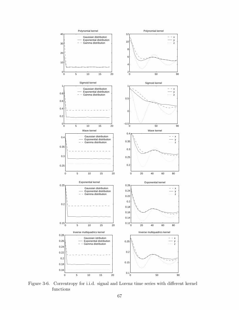
0 5 10 15 200
10
20
30
40Polynomial kernel
0 50 902
4
6
8
10
12Polynomial kernel
0 5 10 15 200
0.2
0.4
0.6
0.8
1Sigmoid kernel
0 50 90−0.5
0
0.5
1Sigmoid kernel
xyz
Gaussian distributionExponential distributionGamma distribution
xyz
Gaussian distributionExponential distributionGamma distribution
0 5 10 15 20
0.25
0.3
0.35
0.4
Wave kernel
0 20 40 60 80
0.2
0.25
0.3
0.35
0.4Wave kernel
0 5 10 15 200.15
0.2
0.25Exponential kernel
0 20 40 60 800.12
0.14
0.16
0.18
0.2
0.22
0.24
0.26Exponential kernel
xyz
Gaussian distributionExponential distributionGamma distribution
xyz
Gaussian distributionExponential distributionGamma distribution
0 5 10 15 20
0.16
0.18
0.2
0.22
0.24
0.26
0.28Inverse multiquadrics kernel
0 50 900.1
0.15
0.2
0.25
Inverse multiquadrics kernel
xyz
Gaussian istributionExponential distributionGamma distribution
Figure 3-6. Correntropy for i.i.d. signal and Lorenz time series with different kernelfunctions
67

λ = 2.5 for exponential kernel and θ = 0.7 for inverse multiquadrics kernel. The
correntropy functions for i.i.d. data of Gaussian, exponential and Gamma distributions
and Lorenz time series are plotted using different kernel function in Fig. 3-6. Notice that
all the kernel functions except polynomial kernel can separate different PDF data. The
sigmoid kernel fails to detect the nonlinear coupling embedded in Lorenz time series.
The wave, exponential and inverse multiquadrics kernels exhibit reasonable performance
compared to Gaussian kernel.
3.2 Frequency-Domain Analysis
We have already presented the definitions and properties of correntropy and centered
correntropy functions in the previous sections. If we view the correntropy and centered
correntropy functions as generalized correlation and covariance functions, certainly
we can proceed to the frequency-domain analysis. Similar to the conventional (power)
spectral density function defined for a wide-sense stationary random processes, we can
also define (correntropy) spectral density function for a correntropy-sense stationary
random processes. Fourier transformation techniques offer an alternative approach to the
time-domain analysis of correntropy for random processes.
Definition: Given a correntropy-sense stationary random process xt, t ∈ T with
centered correntropy function U(τ), the correntropy spectral density function is defined by
P (ω) =
∫ ∞
−∞U(τ)e−jωτdτ, (3–42)
whenever the integral exists. In other word, the correntropy spectral density function is
the Fourier transform of the centered correntropy function.
The variable ω in Eq. (3–42) is usually called the radian frequency and is measured
in radians per second. The frequency ω/2π, denoted as f , is referred to as the “usual”
frequency and measured in hertz(Hz). To convert an expression for the correntropy
spectral density as a function of ω into an expression for the same spectral density as a
function of f , one needs to replace ω by 2πf . Formally, the correntropy spectral density as
68

a function of frequency in Hz is defined by
P (f) =
∫ ∞
−∞U(τ)e−j2πfτdτ. (3–43)
Since P (ω) = FU(τ), we can obviously define the inverse transform of the
correntropy spectral density function, U(τ) = F−1P (ω), as
U(τ) =
∫ ∞
−∞P (ω)ejωτdω/2π (3–44)
=
∫ ∞
−∞P (f)ej2πfτdf. (3–45)
In particular, when the time lag τ = 0, the correntropy spectral spectral density function
becomes
E[κ(xt, xt)]− ExtExt [κ(xt, xt)] = E[‖Φ(xt)‖2]− ‖E[Φ(xt)]‖2 = U(0)
=1
2π
∫ ∞
−∞P (ω)e0dω
=1
2π
∫ ∞
−∞P (ω)dω =
∫ ∞
−∞P (f)df. (3–46)
This equation shows that the difference between the expectation of norm square and
norm square of the expectation of the nonlinearly transformed random process is the total
area under the correntropy spectral density function P (f) of the process. In second-order
random processes analysis, the power in the random process is the total area under the
power spectral density function. By the similar approach, we define the difference between
the expectation of norm square and norm square of the expectation of the nonlinearly
transformed random process, in other word, the centered correntropy at zero lag U(0), as
the correntropy power. From a geometrical perspective, U(0) can also be considered as
“generalized” variance, or “generalized” power, of the nonlinearly transformed random
process in the feature space. Physically, P (ω) represents the density of correntropy
power at frequency ω radians/sec, and P (f) plays the same role for frequency in Hz.
The correntropy power in any frequency band is obtained by integrating the correntropy
69

spectral density function over the range of frequencies that build up the band. Specifically,
the correntropy power in a frequency band from ω1 to ω2 radians/sec, or from f1 to f2 Hz,
is defined as
1
2π
∫ ω2
ω1
P (ω)dω =
∫ f2
f1
P (f)df. (3–47)
The correntropy spectral density function for a correntropy-sense stationary random
process satisfies the following properties:
Property 1: P (ω) = P (−ω), for all ω.
Because U(τ) = U(−τ) for a correntropy-sense stationary random process, we then
have
P (ω) =
∫ ∞
−∞U(τ)e−jωτdτ =
∫ ∞
−∞U(−λ)e+jωλdλ
=
∫ ∞
−∞U(λ)e−j(−ω)λdλ = P (−ω). (3–48)
Property 2: P (ω) = [P (ω)]∗, for all ω.
[P (ω)]∗ denotes the complex conjugate of P (ω). To prove this property, notice that
[P (ω)]∗ =
[∫ ∞
−∞U(τ)e−jωτdτ
]∗=
∫ ∞
−∞U(τ)[e−jωτ ]∗dτ
=
∫ ∞
−∞U(τ)e+jωτdτ =
∫ ∞
−∞U(τ)e−j(−ω)τdτ
= P (−ω) = P (ω). (3–49)
This property shows that the correntropy spectral density function is real.
Property 3: P (ω) ≥ 0, for all ω.
70

Observe that for any T ≥ 0,
0 ≤ E
∥∥∥∥∫ T
0
(Φ(xt)− E[Φ(xt)])e−jωtdt
∥∥∥∥2
= E
⟨[∫ T
0
(Φ(xt)− E[Φ(xt)])e−jωtdt
],
[∫ T
0
(Φ(xs)− E[Φ(xs)])e−jωsds
]∗⟩
= E
∫ T
0
∫ T
0
〈Φ(xt)− E[Φ(xt)], Φ(xs)− E[Φ(xs)]〉 e−jω(t−s)dtds
=
∫ T
0
∫ T
0
U(t− s)e−jω(t−s)dtds.
Hence, this last double integral is nonnegative. Since T ≥ 0, certainly, T−1 is also greater
than 0, and this results in
T−1
∫ T
0
∫ T
0
U(t− s)e−jω(t−s)dtds ≥ 0 (3–50)
for all T ≥ 0. We make a change-of-variable transformation in Eq. (3–50) by letting
t − s = τ . The transformation maps the original region of integration (t, s) : 0 ≤t ≤ T, 0 ≤ s ≤ T onto the region (t, τ) : 0 ≤ t ≤ T, t − T ≤ τ ≤ t. In other
word, the original region of square is changed into a parallelogram, which can also be
decomposed into two regions with G1 = (t, τ) : τ ≤ t ≤ T, 0 ≤ τ ≤ T and
G2 = (t, τ) : 0 ≤ t ≤ T + τ,−T ≤ τ ≤ 0. Then Eq. (3–50) can be rewritten as the sum
of an integral over the region G1 and an integral over the region G2 as follows:
T−1
∫ T
0
∫ T
0
U(t− s)e−jω(t−s)dtds
= T−1
∫ T
0
[∫ T
τ
U(τ)e−jωτdt
]dτ +
∫ 0
−T
[∫ T+τ
0
U(τ)e−jωτdt
]dτ
= T−1
∫ T
0
(T − τ)U(τ)e−jωτdτ +
∫ 0
−T
(T + τ)U(τ)e−jωτdτ
=
∫ T
−T
(T − |τ |)T
U(τ)e−jωτdτ. (3–51)
71

Let us define the function UT (τ) as
UT (τ) =
[1− |τ |
T
]U(τ), |τ | ≤ T
0, |τ | > T(3–52)
Then for any fixed τ , we have
limT→∞
UT (τ) = U(τ). (3–53)
Therefore, the limit of Eq. (3–51) becomes
limT→∞
∫ T
−T
(T − |τ |)T
U(τ)e−jωτdτ = limT→∞
∫ ∞
−∞UT (τ)e−jωτdτ
=
∫ ∞
−∞lim
T→∞UT (τ)e−jωτdτ
=
∫ ∞
−∞U(τ)e−jωτdτ = P (ω). (3–54)
The interchange of order of the limit and the integration is validated by the dominated
convergence theorem [21]. Eq. (3–51) and Eq. (3–54) established that P (ω) is the limit of
a sequence of nonnegative numbers for any ω, and the limit of a sequence of nonnegative
numbers must be nonnegative. Consequently, P (ω) ≥ 0.
72

CHAPTER 4CORRENTROPY ANALYSIS BASED ON RKHS APPROACH
From the definitions of correntropy and centered correntropy functions, we know
that there are two reproducing kernel Hilbert spaces embedded in the correntropy and
centered correntropy functions. The first RKHS is induced by the symmetric positive
definite data independent kernel functions, like the Gaussian kernel, Sigmoid kernel and
others Eq. (3–36) - Eq. (3–41). These kernel functions nonlinearly transform the original
random processes into a high dimensional RKHS, which is called feature space. The linear
operations on the transformed random processes will become nonlinear operations on the
original random processes when mapped back by the inverse nonlinear transformation.
The second RKHS is induced by the symmetric positive definite data dependent
correntropy and centered correntropy functions directly. Unlike the conventional
autocorrelation and covariance functions that operate directly on the original random
processes and determine data dependent RKHS, correntropy and centered correntropy
operate on the expectation of nonlinearly transformed random processes, hence induce
reproducing kernel Hilbert spaces that are very different from the ones determined by data
independent kernel functions and conventional autocorrelation and covariance functions.
The inclusion of data independent kernel functions inside the expectation operation makes
the correntropy and centered correntropy functions different from kernel functions and
expectation operation alone. This also changes the dynamics of the RKHS induced by the
correntropy and centered correntropy and makes it unique.
In this chapter, we investigate the correntropy and centered correntropy functions
from a geometrical perspective by analyzing the reproducing kernel Hilbert spaces induced
by them directly and the one by kernel functions alone. These two approaches to analyze
the correntropy and centered correntropy will lead us to a better understanding of the
geometrical structure of the RKHS induced by kernel functions, correntropy and centered
correntropy respectively.
73

By the Mercer’s theorem, any symmetric positive definite functions possess an
eigen-decomposition. Even without the explicit knowledge of the eigen-functions and
eigen-values, kernel methods solve problems which can be expressed in terms of inner
product because the evaluation of the inner product is equivalent to the value of kernel
function. In this chapter, we present a new method to explicitly build the RKHS with
Gaussian kernel based on polynomial functions. A knowledge of the bases that construct
the RKHS offer a potential applications of RKHS beyond the inner product.
4.1 RKHS Induced by the Kernel Function
By the Mercer’s theorem in chapter 1 Eq. (1–14), any symmetric positive definite
function κ(xt, xs) can be rewritten as an inner product between two vectors in the feature
space, i.e.,
κ(xt, xs) =∞∑
k=0
λkϕk(xt)ϕk(xs)
= 〈Φ(xt), Φ(xs)〉 (4–1)
Φ : xt 7→√
λkϕk(xt), k = 1, 2, . . . , and t ∈ T.
where λk and ϕk are eigen-values and orthogonal eigen-functions for the kernel κ(·, ·)respectively. The nonlinear transformation Φ maps the random process xt : t ∈ T into
another random process Φ(xt) : t ∈ T in the high-dimensional feature space, which is a
reproducing kernel Hilbert space induced by the kernel according to the Moore-Aronzajn
theorem Eq. (1–2). The construction of RKHS based upon the eigen-values and
eigen-functions λk and ϕk follows the same approach from Eq. (1–14) to Eq. (1–20)
by substituting the autocorrelation function R(t, s) with kernel function κ(xt, xs). Notice
that if isotropic kernel functions are used, specifically the Gaussian kernel Eq. (3–36),
wave kernel Eq. (3–39), exponential kernel Eq. (3–40) and inverse multiquadrics kernel
Eq. (3–41), then the norm of transformed random process ‖Φ(xt)‖2 is a constant equals
to κ(0). This shows that the transformed random process Φ(xt) : t ∈ T resides
on the sphere. The isotropic kernel functions transform the random processes such
74

that the instant power become constant. This approach offers potential applications in
communications and signal processing.
The data independent kernel functions include Gaussian kernel, Sigmoid kernel and
others Eq. (3–36) - Eq. (3–42). These data independent kernel functions are embedded
inside the correntropy and centered correntropy functions. An analysis of correntropy and
centered correntropy from kernel perspective offers a new insight.
4.1.1 Correntropy Revisited from Kernel Perspective
According to the inner product expression in Eq. (4–1), we can rewrite the correntropy
in terms of the nonlinear mapping Φ as
V (t, s) = E[〈Φ(xt), Φ(xs)〉]. (4–2)
Likewise the centered correntropy can also be expressed as
U(t, s) = E[〈Φ(xt), Φ(xs)〉]− 〈E[Φ(xt)], E[Φ(xs)]〉
= E [〈Φ(xt)− E[Φ(xt)], Φ(xs)− E[Φ(xs)]〉] (4–3)
It can be seen that the correntropy function is a “conventional” correlation function
for the transformed random process in the high-dimensional RKHS. While the centered
correntropy is nothing but the correntropy for the zero mean (centered) random process
Φ(xt)− E[Φ(xt)] : t ∈ T. This way of defining the generalized correlation and covariance
functions follows the same spirit of the standard correlation and covariance functions.
The high order statistics for any random process in the input space turns out to be the
“second-order” statistics in the feature space. Kernel-based learning algorithms employ the
nonlinear mapping Φ to treat nonlinear algorithms in a linear way if the problems can be
expressed in terms of inner product [49]. This suggests that we can deal with nonlinear
systems efficiently and elegantly in a linear fashion when applying the correntropy and
centered correntropy functions.
75

In fact, all the previous properties of correntropy and centered correntropy functions
in section 2.1 can be derived in a kernel framework. For example, property 3 can be shown
that V (t, t) = E[‖Φ(xt)‖2] which means that V (t, t) is nothing but the expectation of norm
square of transformed random process. The centered correntropy at zero lag U(t, t) can be
rewritten as
U(t, t) = E [〈Φ(xt)− E[Φ(xt)], Φ(xt)− E[Φ(xt)]〉]
= E[‖Φ(xt)− E[Φ(xt)]‖2]
= E[‖Φ(xt)‖2]− ‖E[Φ(xt)]‖2 (4–4)
Therefore, the centered correntropy can be viewed as the expectation of the norm square
of zero-mean (centered) transformed random process or the generalized covariance of
transformed random process. Similarly, property 4 can be cast in terms of the nonlinearly
transformed random process. The inequality can be re-expressed as
E[〈Φ(xt), Φ(xs)〉] <√
E[‖Φ(xt)‖2]E[‖Φ(xs)‖2],
which is called the generalized Cauchy-Schwarz inequality in the reproducing kernel
Hilbert space.
From chapter 3.1, we know that if the random process is pair-wise independent then
the correntropy at non-zero lags becomes the information potential and the centered
correntropy at non-zero lags reduces to zero. Under this condition, the nonlinear
transformed random process becomes “uncorrelated” in the feature space. The condition
of pair-wise independence in the original input space implies pair-wise uncorrelatedness in
the feature space, but not vice versa. This offers correntropy and centered correntropy a
wide range of potential applications in machine learning and signal processing.
The kernel function perspective to correntropy and centered correntropy suggests
that we can treat the nested kernel function inside the expectation operator as an implicit
nonlinear transformation that maps the original random process into the RKHS induced
76
by the kernel function, where the transformed random process resides on the sphere if
isotropic kernel functions are used. Then correntropy and centered correntropy functions
are nothing but “generalized” autocorrelation and covariance functions of the nonlinearly
transformed random process. This nonlinear transformation of random processes brings
a range of advantages, as what have been demonstrated in chapter 2, but also poses
challenges about operations on those transformed random processes since only the inner
product of the transformed random processes in known without any knowledge of the
individual nonlinear transformations. A method of explicit construction of the nonlinear
functionals would alleviate the problem.
4.1.2 An Explicit Construction of a Gaussian RKHS
The Mercer’s theorem does not explicitly provide the basis ϕ that builds the RKHS.
Rather it only offers the inner product of the eigen-functions because it is sufficient for
the statistical learning problems which can be expressed in terms of inner products.
One of the most fundamental issues in learning problems is the selection of the data
representation. In kernel-based learning algorithms, this translates into the choice of the
functionals, or the appropriate feature space RKHS. The reason is that the nonlinear
mapping has a direct impact on the kernel and thus, on the solution of the given learning
problems. Different kernels (polynomial, sigmoid, Gaussian) very likely will result in
different performances. The functional form of RKHS is still of great interest to optimize
performance and to get an insight into the appropriateness of the data representation.
Ultimately, this will allow us to utilize the RKHS structure and expand the class of
algorithms, beyond inner products, that can be developed in kernel space. The advantage
of kernel-based learning algorithms becomes also a disadvantage. The general question
of how to select the ideal kernel for a given problem remains an open issue. Recently,
there have been attempts to explicitly construct an RKHS. A. Rakotomamonjy et al.
proposed a method of building an RKHS and its associated kernels by means of frame
theory [78]. Any vector in that RKHS can be represented by linear combination of the
77

frame elements. But a frame is not necessary linear independent although it results in
stable representation.
In this section, we take the polynomial space approach to construct explicitly
an RKHS associated with one of the most popular kernels, the Gaussian kernel. By
transforming a generalized Fock space [45] with a positive operator, we build an RKHS
associated with Gaussian kernel. The functionals, are explicitly given by the polynomials.
Unlike the Mercer’s theorem approach, these functional are not necessary orthornomal.
More importantly, we can gain control over the dimension of the RKHS by means of
selecting the polynomial degree. The simulation suggests that the effective dimension of
RKHS with Gaussian kernel is relatively small.
The definitions of functionals and inner product of a general Hilbert space are given.
Then, a kernel function is imposed on this general Hilbert space to make it a reproducing
kernel Hilbert space. This approach of building an RKHS with polynomials can also be
found in [45], which is called generalized Fock space. Our contribution is that it is an
RKHS associated with Gaussian kernel that we explicitly construct by introducing new
definitions of functionals and kernel function.
First we construct an inner product space H by defining functionals and inner
product. The evaluation of functional f at any given x is given by
f(x) = e− x2
2σ0
n∑
k=0
fk
k!xk, (4–5)
where σ0 is a constant and (n + 1)-tuple (f0,f1, . . . , fn ) are the coefficients which
uniquely characterize the polynomial f . Then the inner product between any two
functionals f and h can be specified in the form
< f, h >=n∑
k=0
σk
k!fkhk, (4–6)
78

where fk and hk are coefficients for f and h respectively and σ = (σ0, σ1, . . . , σn) is a set
of positive constants chosen a priori. It can be easily seen that this inner product space His complete thus forming a Hilbert space.
In order to make H a reproducing kernel Hilbert space, we impose a kernel function κ
on H in the following form
κ(x, y) = e−x2+y2
2σ0
n∑
k=0
1
k!σk
(xy)k. (4–7)
It can be verified that the Hilbert space H, equipped with such κ, is a reproducing
kernel Hilbert space and the kernel function κ(x, ·) is a reproducing kernel because of the
following two properties of κ(x, y):
1. κ(x, y) as a function of y belongs to H for any fixed x because we can rewrite κ(x, y)
as
κ(x, ·)(y) = e− y2
2σ0
n∑
k=0
(xk
σk· e− x2
2σ0 )
k!yk (4–8)
i.e., the constants (xk/σk · e−x2
2σ0 ), k = 0, 1, . . . , n become the coefficients fk, k =
0, 1, . . . , n in the definition of f , and thus
κ(x, ·) ∈ H. (4–9)
2. Given any f ∈ H, the inner product between reproducing kernel and f yields the
function itself,
< κ(x, ·), f > =n∑
k=0
σk
k!(xk
σk
e− x2
2σ0 ) · fk
= e− x2
2σ0
n∑
k=0
fk
k!xk = f(x). (4–10)
This is so called reproducing property.
The RKHS constructed above has the freedom to choose the degree of functionals,
i.e., the dimension n of the kernel space H. The most interesting case is that we might
79

extend it to an infinite-dimensional RKHS provided that the norm of functional is finite as
n → ∞, i.e., given a sequence of positive weighting constants satisfying certain conditions
σ = (σ0, σ1, . . . ),
‖ f ‖2=< f, f >=∞∑
k=0
σk
k!f 2
k < ∞. (4–11)
Then the functionals, inner product and reproducing kernel in H will be defined by Eq.
(4–5), Eq. (4–6) and Eq. (4–7) with n = ∞.
In the special situation of weights
σk = σk0 , k = 1, 2, . . . (4–12)
where σ0 is a fixed positive constant, then the reproducing kernel Eq. (4–7) in the
infinite-dimensional RKHS becomes
κ(x, y) = e−x2+y2
2σ0
∞∑
k=0
1
k!
(xy
σ0
)k
= e−x2+y2
2σ0 exyσ0
= e− (x−y)2
2σ0 , (4–13)
which is the Gaussian kernel used widely in machine learning, function approximation,
density estimation, support vector machine, and etc. The constant σ0 turns out to be the
kernel width. It controls the norm length of those functionals in RKHS. i.e., the spread of
nonlinear mapped data sample in feature space.
Comparing this method with Mercer’s theorem, we notice that there are two major
differences between them.
1. First, we have given an explicit expression for the functionals in the RKHS
associated with Gaussian kernel in terms of polynomials while Mercer’s theorem
never does that. We can get the exact evaluations for those functionals at each point
80

in the RKHS. This enables us to know exactly the structure of the RKHS associated
with the Gaussian kernel.
2. Second, the functionals we constructed above are not necessary an orthonormal
basis, while the Mercer’s theorem is realized by orthonormalizing the RKHS. This
perspective provides also a general alternative to build an RKHS from known
functionals besides from Mercer’s theorem.
3. Third, we can have control of the dimension of the RKHS by means of selecting the
polynomial degrees n in Eq. (4–7).
The method we constructed an RKHS enables us to have the explicit expression of
the functional in RKHS associated with Gaussian kernel. Hence we can exactly know
the nonlinear mapping Φ used in the kernel-based learning algorithm and so operate
directly with the transformed data to extend the algorithms beyond inner products.
Furthermore, as we have the control of the dimension of the RKHS H, this might help the
computational complexity issue in kernel-based learning algorithms through approximation
of Gaussian kernel by polynomials as indicated in equation Eq. (4–7).
The previous way of explicitly constructing an RKHS by means of polynomial
functions was employed by De Figueiredo [45] which is based on the Fock space. The idea
of Fock space was first proposed by Fock in [79] to be used in quantum mechanics, where
quantum states are described in the way of passing from one single object to collections of
objects. More recently Figueiredo introduced an “arbitrarily weighted Fock space”, which
was called generalized Fock space in [45]. The space is equipped with an appropriate
weighted inner product, thus forming an RKHS. The proposed RKHS has been used in
liearn/nonlinear system and signal analysis, where a number of problems are involving
approximation and inversion of nonlinear functions/functionals, and nonlinear operators.
In the univariate case, a generalized Fock space F n is an RKHS, where the functionals f ,
81

inner product and kernel function F are defined as follows respectively,
f(u) =n∑
k=0
fk
k!uk, (4–14)
< f, h >F =n∑
k=0
σk
k!fkhk, (4–15)
F (u, v) =n∑
k=0
1
k!σk
(uv)k, (4–16)
where the real (n + 1)-tuple (f0,f1, . . . , fn ) completely characterizes f , σ = (σ0, σ1,. . . ,
σn) is a set of positive weighting constants which are chosen a priori according to the
problems under consideration. It can be shown that this generalized Fock space is an
RKHS. Similar to the RKHS H we constructed above, the generalized Fock space F n
has the freedom of choosing the space dimension. The interesting case is that when the
space becomes infinite dimensional while the norm of the functional satisfying the same
condition Eq. (4–11) as n → ∞. Then the kernel function F (u, v), defined by Eq. (4–16),
will become an exponential kernel as n →∞
κ(x, y) = exyσ0 , (4–17)
given the same weights constraint as Eq. (4–12).
It can be noticed that there are similarity and difference between the RKHS H and
the generalized Fock space F n. The definitions for the inner product inside the two spaces
are the same, while the functionals and kernel function are different. The relationship of
the two spaces H and F n is connected by a theorem in [2], which states that if H1 and
H2 are two reproducing kernel Hilbert spaces of the same definitions of inner product,
then there exits a positive operator with bound not greater than 1 that transforms H1
into H2 ⊂ H1. Comparing the definitions of functionals for two spaces, we can see that
the e−x2/2σ0 plays the role of a positive operator with bound not greater than 1, thus
transforming the generalized Fock space F n into H such that H ⊂ F .
82

0 5 10 15 20 25 3010
−35
10−30
10−25
10−20
10−15
10−10
10−5
100
Order n
Squ
are
Err
or
Figure 4-1. Square error between a Gaussian kernel and the constructed kernel in Eq.(4–7) versus the order of polynomials
We present a simple simulation here to show the effectiveness of approximation of the
polynomial functionals to the Gaussian kernel. In the simulation, we calculate the square
error between the Gaussian kernel and the proposed kernel in Eq. (4–7) of order n. The
kernel width is chosen to be 1, and the range of the calculated data is from -5 to 5. The
Fig. 4-1 plots the square error versus order n. The line becomes flat at order 11 is due to
the computation precision of MATLAB. The figure suggests that the effective dimension of
the RKHS with Gaussian kernel is relatively small. With only order 11, we can effectively
approximate the Gaussian kernel by polynomials. This also indicates that for practical
purpose it is sufficient to work with much smaller dimensional space instead of infinite
dimensional space for a Gaussian kernel in kernel-based learning algorithms.
4.2 RKHS Induced by Correntropy and Centered Correntropy Functions
We have seen that the kernel function nested inside the correntropy and centered
correntropy functions uniquely induces a reproducing kernel Hilbert space. The nonlinear
83

transformation Φ maps the original random processes into the high-dimensional RKHS
where the transformed random processes appear on a sphere if isotropic kernel function
is used. The correntropy and centered correntropy can be carried out by operating
on those transformed random processes. However, the correntropy and centered
correntropy functions are symmetric non-negative definite themselves, hence determine
two reproducing kernel Hilbert spaces as well. This perspective is in the same spirit of
RKHS in statistical signal processing, where the autocorrelation and covariance functions
are symmetric non-negative definite thus induce reproducing kernel Hilbert space (refer to
the review in chapter 1.2). All the linear statistical signal processing using autocorrelation
and covariance functions can be also treated as functional operations in RKHS. But the
RKHS induced by correntropy and centered correntropy functions is different from the
one induced by conventional autocorrelation and covariance functions. The RKHS by
conventional autocorrelation and covariance functions is based on second order random
processes, hence suitable for the Gaussian processes. While the RKHS by correntropy and
centered correntropy function includes the high order statistical information of random
processes, hence goes beyond the Gaussian processes. It is conjectured that RKHS by
correntropy and centered correntropy functions might encompass a large class of processes.
From the other perspective, the RKHS by conrrentropy and centered correntropy is also
different from the one by kernel functions. One obvious characteristic is that RKHS
by correntropy and centered correntropy is data dependent while the RKHS by kernel
function is data independent. The inclusion of kernel function inside the expectation
operator makes the correntropy and centered correntropy functions unique. It departs
from the conventional RKHS induced by the autocorrelation and covariance functions
used in statistical signal processing and also the data independent kernel functions used in
kernel machine learning. In this section, we analyze the geometry of RKHS by correntropy
and centered correntropy functions.
84

4.2.1 Geometry of Nonlinearly Transformed Random Processes
Given a random process xt : t ∈ T, we can construct another nonlinearly
transformed random process Φ(xt) − E[Φ(xt)] : t ∈ T, where Φ is the nonlinear
mapping associated with the kernel function Eq. (4–1). The reason to work with the
zero-mean nonlinearly transformed random process shall become clear shortly. Let us
define a linear manifold spanned by the random process Φ(xt) − E[Φ(xt)] : t ∈ T,denoted as L (Φ(xt)− E[Φ(xt)] : t ∈ T), to be the set of all random variables ξ that can be
written as the form
ξ =n∑
i=1
ci (Φ(xti)− E[Φ(xti)]) , (4–18)
for some integer n, real constants c1, . . . , cn, and t1, . . . , tn ∈ T. In other words,
L (Φ(xt)− E[Φ(xt)] : t ∈ T) contains all finite linear combinations of the random variables
Φ(xt) − E[Φ(xt)] : t ∈ T. Close the set in Eq. (4–18) topologically according to the
convergence in the mean using the norm
‖ξ − ζ‖ =√
E [‖ξ − ζ‖2] (4–19)
and denote the set of all linear combinations of random variables and its limit points
by L2 (Φ(xt)− E[Φ(xt)] : t ∈ T). In other words, L2 (Φ(xt)− E[Φ(xt)] : t ∈ T) consists
of all random variables in the linear manifold L (Φ(xt)− E[Φ(xt)] : t ∈ T), together
with all random variables ξ such that there exists a sequence of random variables ξn in
L (Φ(xt)− E[Φ(xt)] : t ∈ T) converging to ξ, in the sense that ‖ξ − ξn‖ =√
E [‖ξ − ξn‖2]
→ 0 as n → 0.
It is well known from the theory of quadratically integrable functions that
L2 (Φ(xt)− E[Φ(xt)] : t ∈ T) forms a Hilbert space if the inner product is the one
corresponding to the norm in Eq. (4–19), namely
〈ξ, ζ〉 = E[〈ξ, ζ〉]. (4–20)
85

Figure 4-2. two vectors in the subspace S
Then by the definition of crosscorrentropy Eq. (3–8), we have
〈ξ, ζ〉 = E[〈ξ, ζ〉]
= E[〈Φ(x)− E[Φ(x)], Φ(y)− E[Φ(y)]〉]
= E[κ(x, y)]− ExEy[κ(x, y)] = U(x, y). (4–21)
In other words, the inner product in L2 (Φ(xt)− E[Φ(xt)] : t ∈ T) is the centered
correntropy function of the original random variables. This definition will bridge the
space L2 (Φ(xt)− E[Φ(xt)] : t ∈ T) and the RKHS induced by the centered correntropy
function.
Now let us define a “generalized” deviation of any random variable ξ in
L2 (Φ(xt)− E[Φ(xt)] : t ∈ T) as
σ(ξ) =√
E[‖ξ‖2] = ‖ξ‖
=√
E[〈Φ(x)− E[Φ(x)], Φ(x)− E[Φ(x)]〉]
=√
E[κ(x, x)]− ExEx[κ(x, x)] =√
U(x, x). (4–22)
86

Consider the subspace S spanned by two random variables x1 and x2 (we drop the
time index here for simplicity without any ambiguity):
S = c1(Φ(x1)− E[Φ(x1)]) + c2(Φ(x2)− E[Φ(x2)]) . (4–23)
Then it makes sense to talk about the angle φ between two vectors ξ1 and ξ2 in S (see Fig.
4-2). By plane trigonometry, we have
σ2(ξ1 − ξ2) = σ2(ξ1) + σ2(ξ2)− 2σ(ξ1)σ(ξ2) cos φ, (4–24)
which is the same as
‖ξ1 − ξ2‖2 = ‖ξ1‖2 + ‖ξ2‖2 − 2〈ξ1, ξ2〉
= ‖ξ1‖2 + ‖ξ2‖2 − 2‖ξ1‖‖ξ2‖ cos φ. (4–25)
Consequently, we have
cos φ =〈ξ1, ξ2〉‖ξ1‖‖ξ2‖ =
U(x1, x2)√U(x1, x1)U(x2, x2)
. (4–26)
The quantity measures the angle between two “vectors” in the subspace S of
L2 (Φ(xt)− E[Φ(xt)] : t ∈ T). In particular, if two vectors are orthogonal, then φ is 90.
If two vectors are in same direction, then φ is 0. Now we are in a position to define the
“generalized” correlation coefficient for any two random variables.
Definition: Given any two random variables x and y, we define a “generalized”
correlation coefficient, named correntropy coefficient as
η =U(x, y)√
U(x, x)U(y, y), (4–27)
where U(x, y) is the centered correntropy function for x and y, and U(x, x) and U(y, y) are
centered correntropy functions for variables themselves.
This definition of correntropy coefficient is in the same spirit of traditional correlation
coefficient, where the standard covariance function has been replaced by “generalized”
87

covariance function, centered correntropy Eq. (3–8), and the standard deviation functions
has been replaced by “generalized” deviation function, square root of centered correntropy
with respect to itself Eq. (4–22). However the difference is striking. Conventional
correlation coefficient only measures the second order similarity between two original
random variables, hence it only requires second order statistics in order to attain 0,
i.e., two random variables are uncorrelated. While the correntropy coefficient measures
high order similarity between two original random variables or “second order similarity”
between two nonlinearly transformed random variables in L2 (Φ(xt)− E[Φ(xt)] : t ∈ T),
therefore it needs high order statistics to attain 0. In fact, by the property 4 in chapter
2.1, the value of correntropy coefficient is between -1 and 1. If two original random
variables are independent, i.e., two nonlinearly transformed random variables by Φ are
“uncorrelated” in RKHS induced by kernel function, then the correntropy coefficient
reduces to 0, which means the two vectors in L2 are orthogonal. If two random variables
are the same, the correntropy coefficient is 1, which means the two vectors are in same
direction. This also explains the reason why we use centered correntropy functions,
not correntropy fucntions, in the definition of correntropy coefficient. The correntropy
coefficient will never attain 0 if correntropy functions are used because V (x, y) is always
greater than 0. The pre-processing of making random processes zero mean is vital to many
conventional statistical signal processing. In our context, since we do not have explicit
knowledge of the mean of nonlinearly transformed random processes, we have to rely on
centered correntropy functions.
Substituting the definition of centered correntropy Eq. (3–8) and approximating the
ensemble average by sample mean, we can obtain an estimate of correntropy coefficient
88

directly from data,
η =
1
N
N∑i=1
κ(xi, yi)− 1
N2
N∑i=1
N∑j=1
κ(xi, yj)
√√√√κ(0)− 1
N2
N∑i=1
N∑j=1
κ(xi, xj)
√√√√κ(0)− 1
N2
N∑i=1
N∑j=1
κ(yi, yj)
, (4–28)
where 1N2
∑Ni=1
∑Nj=1 κ(xi, yj) is called cross information potential between x and y [55],
1N2
∑Ni=1
∑Nj=1 κ(xi, xj) and 1
N2
∑Ni=1
∑Nj=1 κ(yi, yj) are again the information potential
for x and y respectively. This observation suggests a connection between the correntropy
coefficient and the Cauchy-Schwartz independence measure in Eq. (1–34) because both
of them use the information theoretic learning concepts to measure the independence
of two random variables. Moreover, the Cauchy-Schwartz independence measure is an
approximation to the Kullback-Leibler divergence [55], this also suggests the correntropy
coefficient is related to mutual information. These connections need further investigation
in the future work.
4.2.2 Representation of RKHS by Centered Correntropy Function
We have analyzed the geometry of L2 (Φ(xt)− E[Φ(xt)] : t ∈ T), where an inner
product of any two vectors is defined in Eq. (4–21) which turns out to be the centered
correntropy function for the original random processes. In this section, we proceed to
prove that there exist a congruence map between L2 (Φ(xt)− E[Φ(xt)] : t ∈ T) and RKHS
induced by centered correntropy function. Therefore it is sufficient to study the Hilbert
space L2 (Φ(xt)− E[Φ(xt)] : t ∈ T) in this perspective.
First because the centered correntropy function U(t, s) is non-negative definite, it
uniquely determine a reproducing kernel Hilbert space by Moore-Aronszajn Theorem. We
can apply Mercer’s theorem to obtain an eigen-decomposition for the centered correntropy
function as
U(t, s) =∞∑
k=0
θkψk(t)ψk(s) = 〈Ψ(t), Ψ(s)〉, (4–29)
89

where θk and ψk are eigen-values and eigen-functions for the centered correntropy function
respectively.
Then we can define a function g on T as the form of
g(t) =∞∑
k=0
θkakψk(t), (4–30)
where the sequence ak, k = 1, 2, . . . satisfies the following condition
∞∑
k=0
θka2k < ∞. (4–31)
Let H(U) be the set composed of functions g(·) which can be represented in the form
Eq. (4–30) in terms of eigenfunctions ψk and eigenvalues θk of the centered correntropy
function U(t, s). Furthermore we might define an inner product of two functions in H(U)
as
〈g1, g2〉 =∞∑
k=0
θkakbk, (4–32)
where g1 and g2 are of form Eq. (4–30) and ak, bk satisfy property Eq. (4–31). One might
as well show H(U) is complete. Let gn(t) =∑∞
k=0 θka(n)k ψk(t) be a Cauchy sequence
in H(U) such that each sequence a(n)k , n = 1, 2, . . . converges to a limit point ak.
Hence the Cauchy sequence converges to g(t) =∑∞
k=0 θkakψk(t) which belongs to H(U).
Therefore H(U) is a Hilbert space. H(U) has two important properties which make it a
reproducing kernel Hilbert space. First, let U(t, ·) be the function on T with value at s
in T equal to U(t, s), then by the Mercer’s Theorem eigen-expansion for the covariance
function Eq. (4–29), we have
U(t, s) =∞∑
k=0
θkakψk(s), ak = ψk(t). (4–33)
Therefore, U(t, ·) ∈ H(U) for each t in T. Second, for every function g(·) ∈ H(U) of form
given by Eq. (4–30) and every t in T,
〈g, U(t, ·)〉 =∞∑
k=0
θkakψk(t) = g(t). (4–34)
90

By the Moore-Aronszajn Theorem, H(U) is a reproducing kernel Hilbert space with
U(t, s) as the reproducing kernel. It follows that
〈U(t, ·), U(s, ·)〉 =∞∑
k=0
θkψk(t)ψk(s) = U(t, s). (4–35)
Thus H(U) is a representation of the random process xt : t ∈ T with centered
correntropy function U(t, s). One may define a congruence G form H(U) onto
L2 (Φ(xt)− E[Φ(xt)] : t ∈ T) such that
G (U(t, ·)) = Φ(xt)− E[Φ(xt)]. (4–36)
The congruence G can be explicitly represented as
G (g) =∞∑
k=0
akξk, (4–37)
where the set of ξk is an orthogonal random variables belong to L2(Ω,F , P ) and g is any
element in H(U) in the form of Eq. (4–30).
This way of proceed from the L2 (Φ(xt)− E[Φ(xt)] : t ∈ T) to the RKHS induced
by the centered correntropy function is in the same spirit of the method to build RKHS
induced by traditional covariance function from the L2(xt, : t ∈ T) [20, 25]. However we
now deal with the nonlinearly transformed random processes via the Φ.
4.3 Relation Between Two RKHS
There are three spaces we have analyzed so far in this chapter. The first one is the
reproducing kernel Hilbert space induced by the data independent kernel function κ(·, ·),where the nonlinearly transformed random processes reside on the sphere if isotropic
kernel functions are used. The inner product in this RKHS is defined as the kernel
function κ(·, ·). The second space is the L2 (Φ(xt)− E[Φ(xt)] : t ∈ T) which is built
upon the RKHS induced by kernel functions by including all the linear combination of
“zero-mean” nonlinearly transformed random process Φ(xt) − E[Φ(xt)] : t ∈ T and
its limit points. An inner product is defined in this space as the form of Eq. (4–21),
91

which turns out to be the centered correntropy function for the original random processes.
Consequently, L2 (Φ(xt)− E[Φ(xt)] : t ∈ T) is complete and thus forms a Hilbert space.
The last space is the reproducing kernel Hilbert space induced by the centered correntropy
function directly. The inner product is defined as the centered correntropy function, the
Mercer kernel. It is proved that there exists an isometric isomorphism (congruence) map
between the RKHS induced by the centered correntropy function and the Hilbert space
L2 (Φ(xt)− E[Φ(xt)] : t ∈ T). By isometry, it means the inner product definitions for two
spaces are the same. By isomorphism, it means there exists a one-to-one mapping between
two spaces. It is sufficient to study the RKHS determined by the centered correntropy
function by considering the Hilbert space L2 (Φ(xt)− E[Φ(xt)] : t ∈ T). Then the relation
among these three spaces become clear. The kernel operator inside the correntropy
function induces a reproducing kernel Hilbert space. The expectation operator induces
another RKHS which is built upon the first RKHS through the Hilbert space L2 since
RKHS by centered correntropy function is congruence to L2.
This interpretation of three spaces involved in centered correntropy functions offers
insights into the geometric relationship among the different spaces. Certainly, there are
other ways to tackle the task and further investigations are required. First, we applied
Mercer’s theorem to non-negative definite centered correntropy function to come up
with an eigen-decomposition in the previous section. It would further our understanding
if we can gain knowledge of the basis. So it is desired that we might also apply what
we have propose in section 3.1.2 of explicit construction of RKHS by Gaussian kernel
function to build those basis for centered correntropy function explicitly. This will be
part of my future work. Second, what we have presented involves high dimensionality, be
it in RKHS by kernel function or in RKHS by centered correntropy function. The high
dimensionality has its own attractiveness but also poses challenges for data manipulation.
So another research direction is to propose a single dimensional nonlinear transformation
function such that the correlation function of those nonlinearly transformed functions is
92

the centered correntropy function, namely to seek a nonlinear function f such that for a
given random process xt : t ∈ T
E[f(xt)f(xs)] = U(t, s) = E[κ(xt, xs)]− ExtExs [κ(xt, xs)]. (4–38)
It is conjectured that this f function will implicitly embed the data distribution. As
has been pointed out random processes theorem, any give non-negative definite function
determines a Gaussian process such the correlation function for the Gaussian process
equals to that non-negative definite function [74]. It also suggests that this f function
might be related to the gaussianization technique.
93

CHAPTER 5CORRENTROPY DEPENDENCE MEASURE
One of the most important tasks in statistical analysis is to measure the degree of
dependence between random variables. There are numerous measures of dependence
in the literature, mostly based on the distance of the joint probability distribution of
the data and the product of the marginal probability distributions [80]. Some of the
most commonly used measures of bivariate dependence include but are not limited to
the correlation coefficient, Kendall’s τ , Spearmans’ ρs, maximal correlation coefficient,
monotone correlation coefficient, and others. The correlation based dependence measures
only characterize linear relationship between two random variables. [81] proposed a
nonlinear canonical correlation using symmetric nondecreasing functions to quantify
nonlinear dependence without any assumption on the distribution of the random variables.
The dependence measure is also closely related to the measure of amount of
information that one random variable contained about in the other. Because the more
dependent the random variables are, the more information about one ought to be given
by the other and vice versa. Several measures based on information theory have been
proposed in the literature. For example, the mutual information is one well-known
measure which can also be interpreted as the Kullback-Leibler divergence between the
joint probability density functions and the product of the marginal densities [82, 83]. It
turns out that the Kullback-Leibler divergence or mutual information is a special case of
the ϕ-divergence measure when a specific convex function ϕ is chosen [84]. On the other
hand, [58] generalized Shannon’s mutual information as a special norm in the probability
density function space. Silvey’s generalized coefficient [85] uses the Radon-Nikodym
derivative of joint distribution of random variables with respect to the product of their
marginal distributions. Other dependence measures based on information theory include
the relative entropy measure proposed by [86] and others. However Joe’s relative entropy
dependence measure, and almost all other entropies fail to be “metric” since they violate
94

the triangularity rule [87]. In order to overcome this limitation, [87] proposed a metric
measure of dependence to specify the degree of dependence in time series data.
Recently there has been considerable work on using functions in reproducing kernel
Hilbert space (RKHS) to quantify dependence. [52] introduced kernel dependence
functionals in the context of independent component analysis (ICA). The kernelized
canonical correlation is a kernelization of canonical correlation analysis with regularization
on the functionals. It can also be explained as a particular form of nonlinear canonical
correlation where the nonlinear functions have been chosen as functional evaluations in
RKHS [88] based on the representer theorem [49]. The kernel generalized variance is
an extension of kernelized canonical correlation by estimating the spectral norm of the
correlation operator between reproducing kernel Hilbert spaces in the entire spectrum
[52]. Instead of using correlation operator in RKHS, [89] proposed the kernel constrained
covariance and kernel mutual information based on the covariance operator. The kernel
constrained covariance estimates the spectral norm of the covariance operator between
RKHSs. It is been proved that the kernel constrained covariance is zero if and only if
the original random variables are independent provided that the kernel is universal. The
kernel constrained covariance can also be viewed as a maximal correlation coefficient
where the function space has been confined to the reproducing kernel Hilbert space. The
kernel mutual information incorporates the entire spectrum of the covariance operator
between RKHSs and becomes an upper bound of the mutual information estimated with
a Parzen window [89]. These dependence measures based on kernel methods have enjoyed
much success in independent component analysis [52, 88, 89], quantification of generalized
synchronization between chaotic signals [90], and other machine learning application areas.
With the abundance of dependence measures in the literature, one would naturally
ask which measure is best in characterizing the dependence information of the data.
Renyi proposed a set of postulates which should be fulfilled by a suitable dependence
measure [91]. The axiomatic framework by Renyi has drawn much attention ever since.
95

Many modifications, extensions and enrichments for these postulates have appeared in
the literature. One of the major criticisms was that these axioms are too strict for most
dependence measures to fulfill. It has been shown by [91] that out of various dependence
measures only the maximal correlation coefficient satisfied all these properties. The kernel
constrained covariance omits the deterministic dependence and upper bound conditions
in the axiomatic framework in order to efficiently estimate the quantity and apply it to
independent component analysis [89].
In this chapter, we define a new parametric correntropy function as a novel
dependence measure.
5.1 Parametric Correntropy Function
An important observation in the definition of the centered correntropy Eq. (3–8) is
that when two random variables are independent (fX,Y (x, y) = fX(x)fY (y)) the quantity
becomes zero but not vice versa. In order to make it a suitable dependence measure, we
modify the definitions of the centered correntropy and correntropy coefficient so that
it will satisfy the condition of attaining zero if and only if two random variables are
independent.
Definition (Parametric Centered Correntropy) Given two random variables x and y,
the parametric centered correntropy is defined as
Ua,b(x, y) = Ex,y[κ(ax, b + y)]− ExEy[κ(ax, b + y)]
=
∫∫
Ω
κ(ax, b + y)(fX,Y (x, y)− fX(x)fY (y))dxdy,
where fX,Y (x, y) is the joint probability density function (PDF) of random variables x and
y, fX(x) and fY (y) are the marginal PDFs respectively, Ω is the probability space and a
and b are parameters in R.
We present a lemma here stating that the parametric centered correntropy is zero for
all a and b if and only if x and y are independent. First, we employ the Fourier transform
96

for the shift-invariant real valued kernel function as
κ(z) =
∫eiαzµ(dα), (5–1)
where µ is a positive bounded measure. For simplicity we will also assume that the
probability measure µ has moments of all orders so that κ is infinitely differentiable. If the
tail of µ decays sufficiently fast κ can be extended to the entire line.
Lemma (Independence): Suppose the measure µ defining the kernel κ has
support in the entire line. Then Ua,b(x, y) = 0 for all a and b if and only if x and y
are independent.
Proof: The sufficient condition is straightforward. Assume Ua,b(x, y) = 0 for all a and b,
re-write the definition of the parametric centered correntropy as
Ua,b(x, y) =
∫∫
Ω
κ(ax− y − b) dFX,Y (x, y)− dFX(x)dFY (y)
=
∫∫
Ω
κ(ax− y − b)dQ(x, y), (5–2)
where FX,Y (x, y) is the joint cumulative distribution function (CDF), and FX(x) and
FY (y) are the marginal CDFs for x and y respectively. Need to show that dQ(x, y) = 0.
Ua,b(x, y) = 0 for all a and b means∫ ∫
eiα(ax−y)dQ(x, y)e−iαbµ(dα) = 0 for all a and b, in
particular for all b. Hence∫ ∫
eiα(ax−y)dQ(x, y) = 0 µ almost all α. Since support µ = R,
this holds for all α and a. This is easily written as∫
ei(αx+βy)dQ(x, y) = 0 for all α and β.
Conclusion dQ = 0. ¥
We can also parameterize the correntropy coefficient.
97

Definition (Parametric Correntropy Coefficient) Given two random variables x and
y, the parametric correntropy coefficient is defined as
ηa,b(x, y) =Ex,y[κ(ax, b + y)]− ExEy[κ(ax, b + y)]√
E[κ(ax, ax)]− ExEx[κ(ax, ay)]√
E[κ(b + y, b + y)]− EyEy[κ(b + x, b + y)]
=
∫∫
Ω
κ(ax, b + y)(fX,Y (x, y)− fX(x)fY (y))dxdy
√κ(0)−
∫
Ω
κ(ax, ay)fX(x)fX(y)dxdy
√κ(0)−
∫
Ω
κ(b + x, b + y)fY (x)fY (y)dxdy
,
(5–3)
where κ(0) is the value of kernel function when its argument is zero. The absolute value of
the parametric correntropy coefficient is bounded by 1.
Proof (Boundedness of parametric correntropy coefficient): By the eigen-decomposition
of the kernel function Eq. (4–1), we have
|Ex,y[κ(ax, b + y)]− ExEy[κ(ax, b + y)]|
=
∣∣∣∣∣Ex,y
[ ∞∑
k=0
λkϕk(ax)ϕk(b + y)
]− ExEy
[ ∞∑
k=0
λkϕk(ax)ϕk(b + y)
]∣∣∣∣∣
=∞∑
k=0
λk |E[ϕk(ax)ϕk(b + y)]− E[ϕk(ax)]E[ϕk(b + y)]|
=∞∑
k=0
λk |E (ϕk(ax)− E[ϕk(ax)])(ϕk(b + y)− E[ϕk(b + y)])|
≤∞∑
k=0
λk
√var(ϕk(ax))var(ϕk(b + y))
(|cov(XY )| ≤
√var(X)var(Y )
)
≤( ∞∑
k=0
λkvar(ϕk(ax))
)1/2 ( ∞∑
k=0
λkvar(ϕk(b + y))
)1/2
, (Cauchy − Schwartz inequality)
(5–4)
where
∞∑
k=0
λkvar(ϕk(ax)) =∞∑
k=0
λk
(E[ϕ2
k(ax)]− E2[ϕk(ax)]). (5–5)
98

The first term of Eq. (5–5) is
∞∑
k=0
λkE[ϕ2k(ax)] = E[
∞∑
k=0
λkϕ2k(ax)] = κ(0),
and the second term of Eq. (5–5) is
∞∑
k=0
λkE2[ϕk(ax)]
=∞∑
k=0
λk
(∫
Ω
ϕk(ax)fX(x)dx
)2
=∞∑
k=0
λk
(∫
Ω
ϕk(ax)fX(x)dx
)(∫
Ω
ϕk(ay)fX(y)dy
)
=
∫∫
Ω
( ∞∑
k=0
λkϕk(ax)ϕk(ay)
)fX(x)fX(y)dxdy
=
∫∫
Ω
κ(ax, ay)fX(x)fX(y)dxdy
= ExEx[κ(ax, ay)].
Therefore,∞∑
k=0
λkvar(ϕk(ax)) = κ(0)−∫∫
Ω
κ(ax, ay)fX(x)fX(y)dxdy. (5–6)
Likewise
∞∑
k=0
λkvar(ϕk(b + y)) = κ(0)−∫∫
Ω
κ(b + x, b + y)fY (x)fY (y)dxdy. (5–7)
Combining Eq. (5–4), Eq. (5–6) and Eq. (5–7) together, we obtain
|Ex,y[κ(ax, b + y)]− ExEy[κ(ax, b + y)]|
≤(
κ(0)−∫∫
Ω
κ(ax, ay)fX(x)fX(y)dxdy
)1/2 (κ(0)−
∫∫
Ω
κ(b + x, b + y)fY (x)fY (y)dxdy
)1/2
.
Hence the absolute value of the parametric correntropy coefficient is bounded by 1. ¥
5.2 Correntropy Dependence Measure
Based on the parametric correntropy coefficient developed in the previous section,
we formulate a novel dependence measure for two random variables. Renyi gave a set
99

of fundamental principles that a measure of statistical dependence Q(x, y) between two
random variables x and y should satisfy. These include
1. Q(x, y) is well defined,
2. 0 ≤ Q(x, y) ≤1,
3. Q(x, y) = 0 if and only if x and y are independent,
4. Q(x, y) = 1 if and only if y = f(x) or x = g(y), where f and g are Borel measurable
functions.
Renyi showed that one measure satisfying these constraints is
Q(x, y) = supf,g
corr(f(x), g(y)), (5–8)
where f(x) and g(y) must have finite positive variance, and f , g are Borel measurable.
We proposed a dependence measure based on the parametric correntropy coefficient
which satisfies all the desirable properties above.
Definition (Correntropy Dependence Measure) Given two random variables x and
y, the Correntropy Dependence Measure is defined as
Γ(x, y) = supa,b|ηa,b(x, y)|, (5–9)
where ηa,b(x, y) is the parametric correntropy coefficient Eq. (5–3).
The correntropy dependence measure is a suitable statistical measure which fulfills all
the fundamental conditions listed by Renyi.
Proof: First the measure Eq. (5–9) is well defined. Since |ηa,b(x, y)| is between 0 and
1 as proved above, certainly the supreme of |ηa,b(x, y)| is also bounded by 0 and 1. The
independence condition is also trivial. If x and y are independent, |ηa,b(x, y)| = 0, therefore
supa,b |ηa,b(x, y)| = 0. Since
0 ≤ |ηa,b(x, y)| ≤ supa,b|ηa,b(x, y)|,
100

if supa,b |ηa,b(x, y)| = 0, then |ηa,b(x, y)| = 0. Therefore x,y are independent. To check the
condition 4, consider the derivation in the boundedness proof Eq. (5–4). The equalities
achieve if and only if when
ϕk(ax)− E[ϕk(ax)] = α(ϕk(b + y)− E[ϕk(b + y)]), ∀k, (5–10)
and,
E[(ϕk(ax)− E[ϕk(ax)])2] = βE[(ϕk(b + y)− E[ϕk(b + y)])2], ∀k. (5–11)
In fact, both conditions Eq. (5–10) and Eq. (5–11) are equivalent. From the condition Eq.
(5–10), we obtain
ϕk(ax) = Bkϕk(b + y) + Ak, ∀k (5–12)
where Bk and Ak are two constant. Let
f(x) =∞∑
k=0
Ckϕk(ax) =∞∑
k=0
Ck(Bkϕk(b + y) + Ak) = g(y), (5–13)
then x = f−1(g(y)) since functional ϕk is continuous and invertible being the eigen-function
of the positive definite kernel. Therefore we conclude the proof. ¥
Unlike the statistical measure proposed by Renyi Eq. (5–8), the correntropy
dependence measure searches the parameter space for a supreme instead of the entire
function space. Compared to the kernel constrained covariance presented in [89], our
measure does not employ regularization technique because our optimization space
is the one dimensional parameter space. However the kernel constrained covariance
operates on the high-dimensional (possibly infinite dimensional) functional space, therefore
regularization is mandatory in order to make solution achievable. By selecting different
values of parameters a and b, the correntropy dependence measure offers a different scale
value of dependence between random variables x and y. The idea is similar to the concept
of wavelet which provides multi-resolution information about signal frequency.
101

CHAPTER 6CORRENTROPY PRINCIPAL COMPONENT ANALYSIS
Principal component analysis (also known as the Karhunen-Loeve transformation in
communication theory) is a powerful tool for feature extraction and data dimensionality
reduction in statistical pattern recognition and signal processing. It can be easily
performed by eigen-decomposition of the standard covariance matrix or by adaptive
algorithms that estimate principal components [92]. Principal component analysis or PCA
is really an affine transformation of the coordinate system such that the rate of decrease of
data variance is maximized. The projections of the data onto the new coordinate system
are called principal components. These projections represent the data optimally in a
least-square sense. In feature extraction, PCA transforms the data in such a way that a
small number of principal components can represent the data while retaining most of the
intrinsic variance of the data. These are sometimes called factors or latent variables of the
data [93].
While PCA yields a smaller dimensional linear subspace that best represents the full
data according to a minimum-square-error criterion, it might be a poor representation if
the data structure is non-Gaussian. Hence nonlinear component analysis may be needed.
There have been numerous attempts to define nonlinear components analysis in the latest
decades. Nonlinear PCA is generally seen as a nonlinear generalization of standard PCA
[92, 93]. The principal component is generalized from straight lines to curves. Principal
curves were proposed by Hastie [94] to define local directions that pass through the
high density parts of the data set. The principal curves are found through an iterative
algorithm that minimizes the conditional expectation of projections on the curves.
Kramer presented a nonlinear PCA based on auto-associative neural networks. The
auto-associative network performs identity mapping from the input data to the output by
minimizing the square error [95]. Recently, Scholkopf et al applied kernel methodology to
obtain a nonlinear form of PCA [50]. This so called Kernel PCA is one of the kernel-based
102

learning algorithms reviewed in Chapter 1.3. The Kernel PCA nonlinearly maps the
original input data into an infinite dimensional reproducing kernel Hilbert space by the
data independent kernel and solves the eigen-decomposition of the Gram matrix of the
input data in a high-dimensional feature space. The Gram matrix has a dimension given
by the number of samples N . The data projections onto the principal directions of the
Gram matrix, i.e. the inner product in feature space, are carried out by means of kernel
functions in the input space. While the utilization of Mercer kernels provides a tractable
way to compute principal components in the high-dimensional feature space, there are
still problems of interpretation and computation of the large dimensional Gram matrix.
Indeed, the number of eigenfunctions of the Gram matrix is dependent on the number of
data samples N , not the size of the data space L. Moreover computing Gram matrices for
millions of samples in a small, let us say, two dimensional space becomes wasteful.
In this chapter, we propose a new nonlinear PCA technique based on the correntropy
function, called correntropy PCA. The correntropy function quantifies the similarity
between the L different components of the L dimensional input data vector (or the
time structure in a time series) using the statistical data distribution. The correntropy
also utilizes a kernel methodology, but in a different form: by applying the kernel to
pairs of data vector components, a random vector (or stochastic process) is nonlinearly
transformed into a high dimensional function space where the similarity between the
components of the transformed random variables (or stochastic process) can be measured
by the conventional covariance function. The eigen-decomposition of the covariance
of the transformed data yields the principal directions of the nonlinearly transformed
data. These linear principal directions in feature space correspond to nonlinear principal
directions in the input space. These projections can be efficiently computed by utilizing
the correntropy function. That means, if one has one million samples in a two dimensional
space, it is only necessary to solve a two dimensional eigenvector problem on a matrix
103

whose entries are computed from one million samples. In many applications this is a
tremendous computational saving.
Given a set of zero mean vector observations xj, j = 1, . . . , N , xj ∈ RL,∑N
j=1 xj = 0,
correntropy PCA seeks a direction in the feature space such that the variance of the data
projected onto this direction is maximized. Unlike the kernel method which transforms
data into a feature space sample by sample, correntropy PCA maps data component-wise
into a feature space, i.e., the RKHS associated with the centered correntropy function. By
the equation Eq. (4–29),
Ψ : RL 7→ F
x 7→ [Ψ(x1), Ψ(x2), · · · , Ψ(xL)] ,
where xi denotes the ith component of the original input data sample x. This nonlinear
mapping transforms the component-wise data into a high dimensional RKHS which
is associated with the centered correntropy function. By the definition of centered
correntropy function, we have
< Ψ(xi), Ψ(xj) > = U(xi, xj) = Exi,xj[κ(xi, xj)]− Exi
Exj[κ(xi, xj)] (6–1)
=1
N
N∑
k=1
κ(xik, xjk)− 1
N2
N∑
k=1
N∑m=1
κ(xik, xjm), ∀ i, j = 1, 2, ..., L,
where xik is the ith component of the kth input data sample. The expectation runs over all
the data samples.
Then the covariance matrix of the transformed data in the feature space is given by
C =1
L
L∑i=1
Ψ(xi)ΨT (xi)
We now have to find the eigenvalues λ ≥ 0 and non-zero eigenvectors satisfying
Cq = λq.
104

All the solutions q must lie in the span of Ψ(x1), . . . , Ψ(xL), i.e., we q is the form of linear
combination of all the Ψ(x1), . . . , Ψ(xL),
q =L∑
i=1
βiΨ(xi) (6–2)
And we may instead consider the set of equations,
< Ψ(xk), Cq >=< Ψ(xk), λq >, ∀ k = 1, . . . , L. (6–3)
Combining equations Eq. (6–2) and Eq. (6–3), we get
< Ψ(xk),1
L
L∑j=1
Ψ(ji)ΨT (ji) ·
L∑i=1
βiΨ(xi) >
=1
L
L∑j=1
L∑i=1
βi < Ψ(xk), Ψ(xj) >< Ψ(xj), Ψ(xi) >
= λ
L∑i=1
βi < Ψ(xk), Ψ(xi) >, ∀ k = 1, . . . , L. (6–4)
By equation Eq. (6–1), we can define an L× L centered correntropy matrix U by
Uij : = E[κ(xi, xj)]− ExiExj
[κ(xi, xj)] (6–5)
=1
N
N∑
k=1
κ(xik, xjk)− 1
N2
N∑
k=1
N∑m=1
κ(xik, xjm),
∀ i, j = 1, 2, ..., L.
Let k in Eq. (6–4) runs from 1 to L, and write the result in matrix form, we can get
U2β = LλUβ, (6–6)
where β denotes the column vector with entries β1, . . . , βL. It can be shown that the
solutions of equation Eq. (6–6) are equivalent to the solutions to the following eigenvalue
problem,
Uβ = Lλβ, (6–7)
for nonzero eigenvalues.
105

For the purpose of principal component extraction, we need to compute the
projections onto the eigenvectors q in the feature space. Let x be a test point, the
projection of x onto the principal direction mapped back to input space is given by
P (x) =L∑
i=1
βi1
N
N∑j=1
κ(xij, xi), (6–8)
this is so called a nonlinear principal component.
In summary, we need to take the following steps to compute the nonlinear principal
components: (1) compute the correntropy matrix V by equation Eq. (6–5), where the
expected value is substituted by the average, (2) compute its eigenvectors and eigenvalues
through SVD, and (3) compute the projections of a test point onto the eigenvectors by Eq.
(6–8).
We will present two experimental results to show the effectiveness of correntropy
PCA in finding nonlinear principal directions. The first experiment compares the standard
linear PCA and correntropy PCA to extract features from a two dimensional mixture of
Gaussian distributed data. Specifically, the probability density function is a mixture of
Gaussian modes with the following form
f(x) = 1/2(N (m1,Σ1) +N (m2,Σ2)),
where N (m1,Σ1) and N (m2,Σ2) are two Gaussian distributed data with the mean
vectors and variance matrices given by
m1 =
−1
−1
, Σ1 =
1 0
0 0.1
,
m2 =
1
1
, Σ2 =
0.1 0
0 1
.
In Fig. 6-1, we plot the contours of the data and of the largest eigenvalue directions
produced by linear PCA and correntropy PCA respectively. 200 samples are used and
106

−3 −2 −1 0 1 2
−2
−1
0
1
2
3
Linear PCA
X0
X1
−3 −2 −1 0 1 2
−2
−1
0
1
2
3
Correntropy PCA
X0X
1
Figure 6-1. Linear PCA versus correntropy PCA for a two-dimensional mixture ofGaussian distributed data
kernel size is chosen to be 2. The result confirms that linear PCA only provides the linear
directions that maximizes the variance. But since the underlying data is a mixture of
two Gaussian modes, linear PCA fails to consider the directions of the individual modes
but only averages these directions. On the contrary, correntropy PCA is more tuned to
the underlying structure of the data in the input space. correntropy PCA generates a
nonlinear principal direction that follows locally the directions of the individual modes so
that the variance of principal component projected onto this nonlinear curve is maximized.
The experiment shows that correntropy PCAis superior in describing the underlying
structure of the data when compared to the linear PCA method.
Our second experiment compared the kernel PCA, proposed by Scholkopf et al in
[50], with correntropy PCA. We use the same experiment setup as in [50] in order to
illustrate the performance of correntropy PCA. The data is two-dimensional with three
clusters(Gaussian distribution with standard deviation 0.1). The number of data sample
and the kernel size are chosen to be 90 and 0.1 respectively. Since the number of principal
107

−1 −0.5 0 0.5 1−0.5
0
0.5
1
1.5Eigenvalue=22.558
Ker
nel P
CA
−1 −0.5 0 0.5 1−0.5
0
0.5
1
1.5Eigenvalue=20.936
−1 −0.5 0 0.5 1−0.5
0
0.5
1
1.5Eigenvalue=1.794
Cor
rent
ropy
PC
A
−1 −0.5 0 0.5 1−0.5
0
0.5
1
1.5Eigenvalue=0.206
Figure 6-2. Kernel PCA versus correntropy PCA for a two-dimensional mixture ofGaussian distributed data
components for kernel PCA depends on the number of data samples, there are many
eigen-directions in feature space that are difficult to identify in the input space, so we plot
the two principal components with the largest eigenvalues from kernel PCA. However the
number of principal components for correntropy PCA is equal to the dimension of input
space, so there is no ambiguity. Fig. 6-2 shows that both kernel PCA and correntropy
PCA can extract the nonlinear principal components form the data. While kernel PCA
tends to find the local structure for a given data set as the contours circle around different
data clusters suggest, correntropy PCA seeks the underlying global structure of the data
set. The contour in the left bottom plot shows that correntropy PCA can be tuned to the
data structure by changing the kernel size in the Gaussian kernel, and locate the principal
direction.
In experiments comparing the performance of correntropy PCA with standard linear
PCA and kernel PCA for nonlinear feature extraction, we found two advantages of our
method. First, correntropy PCA can be more tuned to the underlying data structure
108

than linear PCA so that it can extract the nonlinear principal components from the data,
very much like principal curves. There is no ambiguity since the number of nonlinear
principal components is the same as the dimensionality of the input space. In kernel PCA
it is very difficult to choose the eigen-directions if we can not visualize the data, since
the eigenvectors project locally to the input space. Therefore, it is not easy to separate
major and minor components. Second, correntropy PCA has a tremendous computational
complexity advantage over kernel PCA. For example, in the second simulation, we only
need to compute an eigen-decomposition for a 2 × 2 matrix using correntropy PCA while
we have to do eigen-decomposition for a 90 × 90 matrix using kernel PCA. As the training
set increases, the computational complexity of kernel PCA will increase dramatically but
the size of the correntropy matrix remains the same.
In this chapter we applied correntropy concepts in principal component analysis. The
approach is based on finding the eigenvectors of the centered correntropy matrix (same
as the dimension of the data) unlike the Gram matrix used by other kernel methods,
where the dimension of the Gram matrix is dependent on the number of the data. Yet,
the final principle curves we get using this method adequately covers the data in the
direction of maximum spread (variance in the feature space). Since we are dealing with
a finite dimensional matrix, we get a number of principle curves equal to the dimension
of the data space, and at the same time the computational complexity is drastically
reduced compared to the kernel methods. In general this approach offers a new method
of analyzing data. The study also suggests that the concept of correntropy can be used
for de-correlating the data in the feature space (whitening), which can be applied in the
context of independent component analysis. The future research will apply correntropy
PCA to real data problem and also compare with other nonlinear principal component
analysis methods.
109

CHAPTER 7CORRENTROPY PITCH DETERMINATION ALGORITHM
7.1 Introduction
Pitch, or the fundamental frequency F0, is an important parameter of speech signals.
Accurate determination of pitch plays a vital role in acoustical signal processing and has
a wide range of applications in related areas such as coding, synthesis, speech recognition
and others. Numerous pitch determination algorithms (PDA) have been proposed in
the literature [96]. In general, they can be categorized into three classes: time-domain,
frequency-domain, and time-frequency domain algorithms.
Time-domain PDAs operate directly on the signal temporal structure. These include
but are not limited to zero-crossing rate, peak and valley positions, and autocorrelation.
The autocorrelation model appears to be one of the most popular PDAs for its simplicity,
explanatory power, and physiological plausibility. For a given signal xn with N samples,
the autocorrelation function R(τ) is defined as
R(τ) =1
N
N−1∑n=0
xnxn+τ , (7–1)
where τ is the delay parameter. For dynamical signals with changing periodicities, a
short-time window can be included to compute the periodicities of the signal within the
window ending at time t as
R(τ, t) =1
N
N−1∑n=0
xnxn+τwt,
where wt is an arbitrary causal window that confines the autocorrelation function into
a neighborhood of the current time. Other similar models can be obtained by replacing
the multiplication by subtraction (or excitatory by inhibitory neural interaction) in the
autocorrelation function such as the average magnitude difference function (AMDF) [97].
Cheveigne proposed the squared difference function (SDF) in [98] as
SDF(τ) =1
N
N−1∑n=0
(xn − xn+τ )2 . (7–2)
110

The weighted autocorrelation uses an autocorrelation function weighted by the inverse
of an AMDF to extract pitch from noisy speech [99]. All these PDAs based on the
autocorrelation function suffer from at least one unsatisfactory fact: the peak corresponding
to the period for a pure tone is rather wide [100, 101]. This imposes greater challenge for
multiple F0 estimation since mutual overlap between voices weakens their pitch cues, and
cues further compete with cues of other voices. The low resolution in pitch estimation
results from the fundamental time-frequency uncertainty principle [102]. To overcome
this drawback, Brown et al. presented a “narrowed” autocorrelation function to improve
the resolution of the autocorrelation function for musical pitch extraction [103]. The
“narrowed” autocorrelation function includes terms corresponding to delays at 2τ , 3τ , etc.,
in addition to the usual term with delay τ as
SL(τ) =1
N
N−1∑n=0
(xn + xn+τ + xn+2τ + · · ·+ xn+Lτ )2 . (7–3)
However it requires an increase in the length of the signal and less precision in time. It
also requires the a priori selection of the number of delay terms L .
Frequency-domain PDAs estimate pitch by using the harmonic structure in the
short-time spectrum. Frequency-domain methodologies include component frequency
ratios, filter-based methods, cepstrum analysis and multi-resolution methods. Pitch
determination algorithms such as harmonic sieve [104], harmonic product spectrum
[105], sub-harmonic summation [106], and subharmonic to harmonic ratio [107] fall
into this category. Most frequency-domain pitch determination methods apply pattern
matching [108]. Others use nonlinear or filtering preprocessing to generate or improve
interpartial spacing and fundamental component cues. The frequency-domain PDAs have
the advantage of efficient implementation with fast Fourier transform and theoretical
strength of Fourier analysis. However one weakness is that they rely on the shape and size
of the analysis window. Selection and adjustment of analysis window remain a problem in
estimation.
111

The time-frequency approach splits the signal over a filter-bank, applies time-domain
methods to each channel waveform, and the results are aggregated over channels. The
summary, or “pooled”, autocorrelation functions across all channels provides pitch
information of the signal. Licklider first presented this idea as a pitch perception model
[109]. Later Lyon and Slaney further developed the methodology and called it cor-
relogram [110, 111]. The correlogram is the first stage processor in a computational
auditory scene analysis (CASA) system [112]. It has also been incorporated into a neural
oscillator to segregate double vowels and multipitch tracking [101, 113]. The strength
of correlogram in pitch estimation is that different frequency channels corresponding to
different signal sources of different pitches can be separated, which makes it useful in
multipitch estimation [101, 114]. Also individual channel weighting can be adapted to
compensate for amplitude mismatches between spectral regions [115].
On the other hand, autocorrelation and power spectrum based pitch determination
algorithms mentioned above only characterizes second-order statistics. In many applications
where non-Gaussianities and nonlinearities are present, these second-order statistical
methodologies might fail to provide all the information about the signals under study.
Higher-order statistics have been used in pitch determination. Moreno et al. applied
higher-order statistics to extract pitch from noisy speech [116]. But only diagonal third
order cumulants were used for simplicity and computational efficiency which is given by
c(k) =1
N
N−1∑n=0
xnxnxn+k, k = 0, · · · , N − 1.
And pitch is found by applying autocorrelation function to the cumulants c(k),
G(τ) =1
2N
N−1∑
k=−(N−1)
c(k)c(k + τ). (7–4)
112

In this chapter, we propose a new pitch determination algorithm based on the
correntropy function defined in the previous chapters,
V (τ) =1
N
N−1∑n=0
κ(xn, xn+τ ). (7–5)
The proposed pitch determination method is applied after the acoustical signal is
processed by an equivalent rectangular bandwidth (ERB) filter bank in the time domain.
The ERB filter bank acts as a cochlear model to transform a one dimensional acoustical
signal into a two dimensional map of neural firing rate as a function of time and place
[111]. The correntropy function for each channel is calculated and the summation across
all the channels provides the pitch information. As a novel “self-similarity” measure,
correntropy is able to offer much better resolution than the conventional autocorrelation
function in pitch estimation. Moreover, our pitch determination algorithm can segregate
double vowels without applying any complex model such as a neural oscillator [101].
7.2 Pitch Determination based on Correntropy
The structure of the correntropy definition seems very appropriate to quantify
similarity in time, in a manner that is biologically plausible, that is, it can be implemented
at neuronal level . Its argument is sensitive to differences in time instances as correlation,
but instead of being linear across differences, there is an intermediate nonlinear transformation
that gives more emphasis to values that are closer together. Neurons are known to be very
sensitive to time differences, but their highly nonlinear response may also emphasize
similarity at the close range. In the context of pitch determination, the correntropy
function might as well estimate the pitch information of the signal similar to the
autocorrelation function. However, compared to the autocorrelation function model,
our pitch determination algorithm based on the correntropy function offers much better
resolution and enhances the capacity of estimating multiple pitches. Since correntropy
creates many different harmonics of each resonance present in the original time series
due to the nonlinearity of the kernel function, it may also be useful for perceptual pitch
113

0 50 100 150 200 250Time (lag) / samples
Cor
rent
ropy
Nar
row
ed
corr
elat
ion
Cor
rela
tion
Figure 7-1. Autocorrelation, narrowed autocorrelation with L = 10 and correntropyfunctions of a sinusoid signal.
determination. To illustrate this, we compare the conventional autocorrelation Eq. (7–1),
narrowed correlation Eq. (7–3) and correntropy functions Eq. (7–5) for a simple sinusoid
signal. Fig. 7-1 plots three functions in the lag with respect to the delay lag in the time
domain. All three functions are able to peak at the same delay lag corresponding to the
period of the sinusoid signal. However it is evident that the peaks obtained from the
correntropy function are much narrower and sharper than those from the conventional
autocorrelation and narrowed autocorrelation functions. In Fig. 7-2, we present the
Fourier transform of each function. The ordinary autocorrelation function only exhibits
one harmonic and the narrowed autocorrelation produces 10 harmonics which is equal
to the number of terms L used in Eq. (7–3). The correntropy function places even more
energy at higher harmonics in frequency. The narrowness of correntropy function in the
time domain implies the rich harmonics present in the frequency domain. This is due to
the nonlinear exponential function included in the definition of the correntropy function.
It should also be noticed that there is a connection between the correntropy function
Eq. (7–5) and the square difference function Eq. (7–2). The correntropy function also
uses inhibitory neural interaction model instead of excitatory one with a Gaussian kernel
function, but it nonlinearly transforms the subtraction of the signals by the exponential
114

0 5 10 15 20 25 30 35 40Frequency (Hz)
Cor
rent
ropy
Nar
row
ed
corr
elat
ion
Cor
rela
tion
Figure 7-2. Fourier transform of autocorrelation, narrowed autocorrelation with L = 10and correntropy functions of a sinusoid signal.
function. From another perspective, the correntropy function includes the scaled square
different function as an individual term for k = 1 in the summation of Eq. (3–11). But it
contains more information with other higher-order moment terms.
Our pitch determination algorithm first uses cochlear filtering to peripherally
process the speech signal. This is achieved by a bank of 64 gammatone filters which
are distributed in frequency according to their bandwidths [117]. The impulse response of
a gammatone filter is defined as
q(t) = tn−1e−2πat cos(2πf0t+ψ),
where n is the filter order with center frequency at f0 Hz, ψ is phase, and a is bandwidth
parameter. The bandwidth increases quasi-logarithmically with respect to the center
frequency. The center frequencies of each filter are equally spaced on the equivalent
rectangular bandwidth scale between 80 Hz and 4000 Hz [118]. This creates a cochleagram,
which is a function of time lag along the horizontal axis and cochlear place, or frequency,
along the vertical axis. The cochlear separates a sound into broad frequency channels
while still contains the time structure of the original sound. It has served as a peripheral
115

0 2 4 6 8 10 12Time (lag) /ms
Figure 7-3. Correlogram (top) and summary (bottom) for the vowel /a/.
pre-process in the computational auditory scene analysis (CASA) model [112], and used
extensively in pitch determination [101, 119].
The periodicity analysis is done by computing the correntropy function at the output
of each cochlear frequency channel,
Vi(τ) =1
N
N−1∑n=0
κ(xin, xi
n+τ ), (7–6)
where i stands for channel number and zn is the cochlear output. The kernel bandwidth
is determined using Silverman’s rule [120]. The time lag τ is chosen long enough to
include the lowest expected pitch. Generally it is set at least 10ms throughout the
paper. In this way, a picture is formed with horizontal axis as correntropy lags and
vertical axis as cochlear frequency. We name it correntropy-gram, which literally means
“pictures of correntropy”. If a signal is periodic, strong vertical lines at certain correntropy
lags appear in the correntropy-gram indicating times when a large number of cochlear
116

0 2 4 6 8 10 12Time (lag) /ms
Figure 7-4. Autocorrelation (top) and summary (bottom) of third order cumulants for thevowel /a/.
channels are firing synchronously. While the horizontal bands signify different amounts
of energy across frequency regions. The correntropy-gram is similar to the correlogram in
structure but different in content. In order to reduce the dynamic range for display in the
correntropy-gram, the correntropy functions should be normalized such that the zero lag
value is one as given by the following formula,
Ci(τ) =
1
N
N−1∑n=0
κ(xin, xi
n+τ )−1
N2
N−1∑n,m=0
κ(xin, xi
m+τ )
√√√√V (0)− 1
N2
N−1∑n,m=0
κ(xin, x
im)
√√√√V (0)− 1
N2
N−1∑n,m=0
κ(xin+τ , x
im+τ )
,
where V (0) is the value of correntropy when lag τ = 0. The numerator is called the
centered correntropy which takes out the mean value of the transformed signal in the
RKHS. C(τ) is also called correntropy coefficient that has been applied to detect nonlinear
dependence among multichannel biomedical signals [121].
117

0 2 4 6 8 10 12Time (lag) /ms
Figure 7-5. Narrowed autocorrelation (top) and summary (bottom) for the vowel /a/.
In order to emphasize pitch related structure in the correntropy-gram, the correntropy
functions are summed up across all the channels to form a “pooled” or “summary”
correntropy-gram,
W (τ) =∑
i
Vi(τ).
The summary correntropy-gram measures how likely a pitch would be perceived at a
certain time lag. The pitch frequency can be obtained by inverting the time delay lag. In
our experiment, the summary of correntropy functions is first normalized by subtracting
the mean and dividing by the maximum absolute value. The position of pitch can be
picked by various peak-picking algorithms to identify local maximum above the pre-defined
threshold. Here we calculate the first derivative and mark the position when the value
changes from positive to negative as a local maximum.
Compared to the conventional correlogram model [101, 119], [122], our pitch detector
is able to locate the same period information as the correlogram, but has much narrower
118

0 2 4 6 8 10 12Time (lag) /ms
Figure 7-6. Correntropy-gram (top) and summary (bottom) for the vowel /a/.
peaks. Hence the proposed method enhances the resolution of pitch determination.
Furthermore, since the correlogram estimates the likelihood that a pitch exists at a certain
time delay, the summary correlogram may generate other “erroneous” peaks besides
the one corresponding to the pitch period [111]. while the summary correntropy-gram
suppresses values that are dissimilar at all other time delays by the exponential decay
of the Gaussian function and only peaks at the one corresponding to the pitch period.
For mixtures of concurrent sound sources with different fundamental frequencies, the
summary correlogram usually fails to detect multiple pitches without further nonlinear
post-processing. But the summary correntropy-gram is able to show peaks at different
periods of each source. These characteristics of the proposed method suggest a superiority
of the correntropy function over the autocorrelation function in pitch determination.
Moreover, the computational complexity of our method, whether the correntropy
function Eq. (7–6) or the correntropy coefficient Eq. (7–7), remains similar to the
119

0 2 4 6 8 10 12Time (lag) /ms
Figure 7-7. Correlogram (top) and summary (bottom) for a mixture of vowels /a/ and/u/.
correlogram. Although there are double summations in the correntropy coefficient, the
computational complexity can be reduced to O(N log N) using the Fast-Gauss transform
[123]. However, the ”narrowed” autocorrelation function increases computational
complexity by including more delay terms.
7.3 Experiments
In this section, we present three experiments to validate our method. In the first
two simulations, we compare our method with the conventional autocorrelation function
[119], the third order cumulants function [116], and the narrowed autocorrelation function
[103] in determining pitches for a single speaker and two combined speakers uttering
different vowels. The synthetic vowels are produced by Slaney’s Auditory Toolbox [124].
For a fair comparison, we did not apply any post-processing on the correlogram as was
used in [119]. The conventional autocorrelation function Eq. (7–1), autocorrelation of
third order cumulants functions Eq. (7–4), narrowed autocorrelation functions Eq. (7–3)
120

0 2 4 6 8 10 12Time (lag) /ms
Figure 7-8. Third order cumulants (top) and summary (bottom) for a mixture of vowels/a/ and /u/.
and correntropy functions Eq. (7–6) are presented after the same cochlear model. In the
third experiment, the proposed method is tested using Bagshaw’s database which is a
benchmark for testing PDAs [125].
7.3.1 Single Pitch Determination
Fig. 7-3 to Fig. 7-6 present the pitch determination results for a single synthetic
vowel /a/ with fundamental frequency at 100Hz. The upper plots are the images of
correlation functions, autocorrelations of third order cumulants, narrowed autocorrelations,
and correntropy functions after the same cochlear model respectively. The bottom
figures are the summaries of those four images. The kernel size σ in the Gaussian kernel
has been chosen to be 0.01 (we will discuss further kernel size selection in Sec. 8.3)
and L = 10 in the narrowed autocorrelation function Eq. (7–3). The conventional
autocorrelation, third order cumulants and narrowed autocorrelation are all able to
produce peaks at 10ms corresponding to the pitch of the vowel. But they also generate
121

0 2 4 6 8 10 12Time (lag) /ms
Figure 7-9. Narrowed autocorrelations (top) and summary (bottom).
other erroneous peaks which might confuse pitch determination. On the contrary, the
summary of correntropy-gram provides only one single and narrow peak at 10ms which
is the pitch period of the vowel. And the peak is much narrower than those obtained
from other methods. The correntropy-gram clearly shows a single narrow stripe across all
the frequency channels which concentrates most of the energy. It is the indication of the
fundamental frequency.
The fine structure of hyperbolic contours can also be clearly seen in the correntropy-gram.
Its power spectrum energy spreads equally at all the harmonics. The rows of white spots
across the correntropy-gram reflect the periodic structure. Particularly, the second
harmonic shows two peaks during the time interval when the fundamental frequency
exhibits one. This fine structure is the result of correntropy’s ability to contain all the
harmonics of signal. However, the correlogram yields a much wider spread of energy across
the frequency channels. The image with the autocorrelations of the third order cumulants
122

0 2 4 6 8 10 12Time (lag) /ms
Figure 7-10. Correntropy-gram (top) and summary (bottom) for a mixture of vowels /a/and /u/.
fail to present such structures. Although, the image of the narrowed autocorrelation
functions is able to show some hyperbolic contours, the white vertical stripe at the
fundamental frequency is much wider than that of the correntropy-gram and there are
other white spots in the high frequency channels. These result in the wide peak at 10ms
and other erroneous peaks in the summary of the narrowed autocorrelation functions.
Our proposed method clearly outperforms the conventional autocorrelation function,
third order cumulants method and narrowed autocorrelation function in single pitch
determination case.
7.3.2 Double Pitches Determination
In this example, we consider pitch determination for a mixture of two concurrent
synthetic vowels with /a/ (F0 = 100 Hz) and /u/ (F0 = 126 Hz) which are separated
by four semitones. We compare the same four methods as the experiment above to
123

0 0.1 0.2 0.3 0.4 0.5 0.6 0.7 0.8 0.9 10
0.1
0.2
0.3
0.4
0.5
0.6
0.7
0.8
Probability of false alarm
Pro
babi
lity
of d
etec
tion
correntropynarrowed correlationcorrelationcumulants
Figure 7-11. The ROC curves for the four PDAs based on correntropy-gram,autocorrelation, narrowed autocorrelation (L = 15), and autocorrelationof 3rd order cumulants in double vowels segregation experiment.
demonstrate that the correntropy function is able to determine two pitches presented in
the mixture of two vowels.
Fig. 7-7 to Fig.7-10 present the simulation results. The correlogram method result
shown in Fig. 7-7 only shows one peak corresponding to the pitch of the vowel /a/ while
no indication of the other vowel /u/ at time of 7.9ms is provided. The summary of
correlogram resembles that of single vowel case in Fig. 7-3. The third order cumulants
method in Fig. 7-8 fails to detect two pitches in the mixture signal. Although there
are two small peaks at 10ms and 7.9ms which correspond to the two pitch periods
respectively, their amplitudes are not large enough to be reliably detected. In Fig. 7-9,
the summary of narrowed autocorrelation functions with L = 15 is able to produce only
one peak at 10ms corresponding to the pitch period of vowel /a/, but there is no peak
at 7.9ms. There are white spots in the low frequency channels in the image of narrowed
autocorrelation functions which are the indications of the second vowel /u/. However,
the amplitude is too small compared with that of vowel /a/ and the information is lost
in the summary plot. A complex neural network oscillator has been used to separate the
124

0 0.25 0.5 1 2 40
10
20
30
40
50
60
70
80
F0 difference (semitones)
Bot
h vo
wel
s co
rrec
t (%
)
correntropyneural oscillator
Figure 7-12. The percentage performance of correctly determining pitches for both vowelsfor proposed PDA based on correntropy function and a CASA model.
channels dominated by different voices, and the summaries of individual channels are able
to produce peaks corresponding to different vowels [101].
On the other hand, our method is able to detect two pitches from the mixture of two
vowels. The kernel size σ is set to 0.07 in this experiment. The correntropy-gram in Fig.
7-10 shows a white narrow stripe across high frequency channels at 10ms corresponding
to the pitch period of the vowel /a/. These channels have center frequencies close to
the three formant frequencies of vowel /a/ (F1 = 730Hz, F2 = 1090Hz, F3 = 2440Hz).
The hyperbolic structure can still be seen in the high frequency channels, but the lower
frequency channels have been altered by the presence of vowel /u/. The three high energy
white spots appear along the frequency channels centered at 300Hz which is the first
formant of vowel /u/. The second white spot locates at 7.9ms matches the pitch period of
vowel /u/. In the summary of correntropy-gram, the first peak at 10ms corresponds to the
pitch period of vowel /a/. It is as narrow as the one in the single vowel case in Fig. 7-6.
The second peak appears at 8.2ms which is only 4Hz off the true pitch frequency (126Hz).
It is much less than the 20% gross error pitch determination evaluation criterion [126]
or 10Hz gross error [99]. The second peak is also much wider than the one at 10ms. The
125

0 2 4 6 8 10 12Time (lag) /ms
σ = 1
σ = 0.1
σ = 0.01
σ = 0.001
Figure 7-13. Summary of correntropy functions with different kernel sizes for a singlevowel /a/.
amplitude for the peak at 8.2ms is also smaller than that of peak at 10ms since the energy
ratio is 5.2 times higher for vowel /a/. The pitch shift and peak broadening phenomenon
is due to the fact that vowel /a/ dominates the mixture signal and it generates spurious
peaks which blur that of vowel /u/. However, it is remarkable that our method, with
the proper kernel size, is able to detect two pitches while all other algorithms fail in this
experiment. This simulation clearly demonstrates the superiority of our method over the
conventional correlogram, third order cumulants and narrowed correlation approaches for
multipitch determination.
7.3.3 Double Vowels Segregation
To further investigate the performance of the proposed PDA, we generate a set
of three vowels: /a/, /u/ and /i/ using Slaney’s Auditory Toolbox. Each vowel is
synthesized on 5 pitches corresponding to differences of 0.25, 0.5, 1, 2 and 4 semitones
from 100Hz, and the duration is 1s each. For every mixture of double vowels, one is always
with the fundamental frequency at 100Hz, and the other constituent can be any vowel
at any pitch value. In total, we have 45 mixtures of different combinations of vowels
with different pitch values (3 vowels × 3 vowels × 5 pitches). The detection functions
from each of four methods above have been normalized to 0 and 1. A threshold varies
126

between 0 and 1 to decide the peaks. If the difference between the detected pitch and
reference is within a certain tolerance, the right pitch is detected. Since the minimum
distance in this experiment is 0.25 semitone from 100Hz, which is 1.45 Hz, we select the
tolerance to be 0.725Hz. Fig. 7-11 plots the ROC curves for the four pitch determination
algorithms based on correntropy function, autocorrelation, narrowed autocorrelation and
autocorrelation of third order cumulants. It clearly shows that our method outperforms
the other three in double-vowel pitch detection. However, none is able to get 100%
detection. Notice that the ROC curve for correntropy function contains many points of
zero probability of false alarm, up to 45% of correct detection. This is due to the fact
that correntropy function is able to suppress other erroneous peaks which are away from
pitch positions and concentrate energy around fundamental frequencies. The performance
of autocorrelation and third order cumulants are below 50% detection rate, irrespective
of the number of false alarms generated, which means that most often the second largest
peak is an harmonic of the highest pitch. This is not surprising since both functions fail to
present two peaks for most mixtures in this experiment.
We also present the vowel identification performance to examine the discriminating
ability of correntropy function at different semitones for the mixture of double vowels.
In the experiment, the threshold is chosen such that the first two peaks are detected.
We compare our results with a computational auditory scene analysis (CASA) model
with a network of neural oscillators [101] in Fig. 7-12. The CASA model outperforms
our method at 0.25, 0.5 and 0.5 semitones of F0 differences since it uses a sophisticated
network of neural oscillators to assign different channels from ERB filter bank outputs
to different vowels. Our method is just based on the simple summary function of
correntropy-gram. The closer the two fundamental frequencies of two vowel become, the
harder for correntropy function to produce two distinct peaks corresponding to different
pitches. However, our method obtains comparable results to CASA model at 2 and 4
semitones of F0 differences. It suggests that our simple model is able to produce similar
127

0 2 4 6 8 10 12Time (lag) /ms
σ = 1
σ = 0.3
σ = 0.07
σ = 0.001
Figure 7-14. Summary of correntropy functions with different kernel sizes for a mixture ofvowels /a/ and /u/.
results for double vowel segregation of 2 and 4 semitones of F0 differences compared to
the sophisticated CASA model. This certainly shows our technique is very promising.
7.3.4 Benchmark Database Test
We test our pitch determination algorithm with Bagshaw’s database [125]. It contains
7298 males and 16948 females speech samples. The groundtruth pitch is estimated at
reference points based on laryngograph data. These estimates are assumed to be equal
to the perceived pitch. The signal is segmented into 38.4ms duration centered at the
reference points in order to make the comparisons between different PDAs fair. The
sampling frequency is 20kHz. The kernel size is selected according to Silverman’s rule for
different segments. We use equation Eq. (7–7) to calculate the normalized correntropy
functions such that the summary correntropy function at zero lag is unit. Since the pitch
range for male speaker is 50-250 Hz and 120-400 Hz for female speaker, the PDA searches
local maximums from 2.5 ms above in the summary correntropy function. We set the
threshold to be 0.3 by trial and error so that every local maximum which exceeds 0.3 will
be detected as a pitch candidate.
Table 7-1 summarizes the performance of various PDAs which are taken from [126],
[127]. The performance criterion is the relative number of gross error. A gross error occurs
128

Table 7-1. Gross error percentage of PDAs evaluation
Male FemalePDA High Low High Low Weighted
(%) (%) (%) (%) Mean (%)
HPS 5.34 28.20 0.46 1.61 11.54SRPD 0.62 2.01 0.39 5.56 4.95CPD 4.09 0.64 0.61 3.97 4.63FBPT 1.27 0.64 0.60 3.35 3.48IPTA 1.40 0.83 0.53 3.12 3.22PP 0.22 1.74 0.26 3.20 3.01
SHR 1.29 0.78 0.75 1.69 2.33SHAPE 0.95 0.48 1.14 0.47 1.55eSRPD 0.90 0.56 0.43 0.23 0.90
Correntropy 0.71 0.42 0.35 0.18 0.71
when the estimated fundamental frequency is more than 20% off the true pitch value.
The percent gross errors by gender and by lower or higher pitch estimates with respect
to the reference are given in Table 7-1. The weighted gross error is calculated by taking
into account the number of pitch samples for each gender. It clearly shows that for this
particular database correntropy based PDA outperforms others.
7.4 Discussions
In all the previous experiments, a specific kernel size σ in the Gaussian kernel Eq.
(3–3) needs to be selected by the user (free parameter). Actually, the kernel size plays an
important role in the performance of our method since it determines the scale at which
the similarity is going to be measured. It has been shown that kernel size controls the
metric of the transformed signal in the RKHS [65]. If the kernel size is set too large, the
correntropy function approaches the conventional correlation function and fails to detect
any nonlinearity and higher order statistics intrinsic to the data; on the other hand, if
the kernel size is too small, the correntropy function loses its discrimination ability. One
practical way to select the kernel size is given by the Silverman’s rule [120]
σ = 0.9AN−1/5,
129

where A is the smaller value between standard deviation of data samples and data
interquartile range scaled by 1.34, and N is the number of data samples.
To illustrate the effect of different kernel sizes, we simulate the summary of
correntropy functions for the same experiments setup in Sec. 8.2 with different kernel
sizes in Fig. 7-13 and Fig. 7-14. It can be seen that if the kernel size is large, σ = 1 here,
the summaries of correntropy functions approach those of correlation functions shown in
Fig. 7-3 and Fig. 7-7. As kernel size approaches the kernel size given by Silverman’s rule,
σ = 0.01 for the single vowel /a/ case and σ = 0.07 for a mixture of /a/ and /u/, the
summary of correntropy functions starts to present a large and narrow peak corresponding
to the pitch of vowel /a/ and show the other vowel /u/. If the kernel size is too small,
σ = 0.001 here, the summary of correntropy functions loses its ability to present two
vowels. This is shown in the bottom plot of Fig. 7-14.
7.5 Conclusion
A novel pitch determination algorithm is proposed based on the correntropy function.
The pitch estimator computes the correntropy functions for each channel of an ERB filter
bank, and adds across all the channels. Simulations on single and double vowel cases
show that the proposed method exhibits much better resolution than the conventional
correlation function, third order cumulants method and narrowed correlation function in
single and double pitches determination. This suggests that correntropy can discriminate
better pitch when two different speakers speak in the same microphone. This is essential
in computational auditory scene analysis (CASA). Although these results are preliminary
and much further work is needed to evaluate the methods, this technique seems promising
for CASA. The automatic selection of the kernel size or of a multiple kernel size analysis
need to be further investigated to automate the pitch determination algorithm. The
future work also includes incorporating correntropy-gram channel selection to enhance the
discriminating ability of proposed method in multiple pitches determination. A benchmark
database test for various PDAs shows that the proposed PDA outperforms some others
130

with available results for this dataset. Since correntropy creates many different harmonics
of each resonance present in the original time series due to the nonlinearity, it may also be
useful for perceptual pitch determination.
131

CHAPTER 8CORRENTROPY COEFFICIENT AS A NOVEL SIMILARITY MEASURE
In this chapter, we apply the proposed correntropy coefficient (4–27) to characterize
the similarity between multi-channel signals. Preliminary experiments with simulated data
and multichannel electroencephalogram (EEG) signals during behavior studies elucidate
the performance of the new measure versus the well established correlation coefficient.
8.1 Introduction
Quantification of dynamical interdependence in multi-dimensional complex systems
with spatial extent provides a very useful insight into their spatio-temporal organization.
In practice, the underlying system dynamics are not accessible directly. Only the
observed time series can help decide whether two time series collected from the system
are statistically independent or not and further elucidate any hidden relationship
between them. Extracting such information becomes more difficult if the underlying
dynamical system is nonlinear or the couplings among the subsystems are nonlinear and
non-stationary.
There has been extensive research aimed at detecting the underlying relationships
in multi-dimensional dynamical systems. The classical methodology employs a linear
approach, in particular, the cross correlation and coherence analysis [128]. Cross
correlation measures the linear correlation between two signals in the time domain,
while the coherence function specifies the linear associations in the frequency domain by
the ratio of squares of cross spectral densities divided by the products of two auto-spectra.
There have been several extensions of correlation to more than two pairs of time series
such as directed coherence, directed transfer functions and partial directed coherence [129].
Unfortunately, linear methods only capture linear relationships between the time series,
and might fail to detect nonlinear interdependencies between the underlying dynamical
subsystems.
132
Nonlinear measures include mutual information and state-space methods. One
technique is the generalized mutual information function [130]. However, a large quantity
of noise-free stationary data is required to estimate these measures based on information
theory, which restricts their applications in practice. Another method is the phase
synchronization where the instantaneous phase using Hilbert transforms is computed
and interdependence is specified in terms of time-dependent phase locking [131]. The
state-space methodologies include similarity-index and synchronization likelihood. The
similarity-index technique and its modifications compute the ratio of average distances
between index points, their nearest neighbors and their mutual nearest ones [132, 133].
Stam et al. proposed the synchronization likelihood to offer a straightforward normalized
estimate of the dynamical coupling between interacting systems [134]. There are several
drawbacks associated with these techniques based on state space embedding. Estimating
the embedding dimension of times series corrupted by measurement noise for a valid
reconstruction, searching a suitable neighborhood size and finding a constant number
of nearest neighbors are a few of many constraints that severely affect the estimation
accuracy.
In this chapter, we use the correntropy coefficient Eq. (4–27) as a novel similarity
measure to quantify the inter-dependencies among multi-channel signals. In practice, the
estimate of correntropy coefficient Eq. (4–28) is calculated between two time series of
interests to measure the similarity.
8.2 Experiments
We test the correntropy coefficient on simulated data set and real world EEG signals
in the experiments.
8.2.1 Two Unidirectionally Coupled Henon maps
First, we test two unidirectionally coupled Henon maps which has been extensively
used to validate many synchronization measure in the literature [133, 134]. We apply
the correntropy coefficient in detecting nonlinear interdependence of two unidirectionally
133

coupled Henon maps defined as
x1(n + 1) = 1.4− x21(n) + bxx2(n) (8–1)
x2(n + 1) = x1(n) (8–2)
for the driver, represented as system X, and
y1(n + 1) = 1.4− [Cx1(n) + (1− C)y1(n)]y1(n) + byy2(n) (8–3)
y2(n + 1) = y1(n) (8–4)
for the response, represented as system Y. System X drives system Y with nonlinear
coupling strength C. C ranges from 0 to 1 with 0 being no coupling and 1 being complete
coupling. Parameters bx and by are both set to 0.3 as canonical values for the Henon map
when analyzing identical systems, and to 0.3 and 0.1 respectively for nonidentical ones.
For each coupling strength, we discard the first 10000 iterated time series as transient
and obtain the next 500 data points for experiments. The correntropy coefficient η is
calculated between the first component of system X, x1, and the first component of system
Y, y1.
In the following simulations, we aim to address these questions: (1) whether
correntropy coefficient increases when the coupling strength C between X and Y for
both identical and nonidentical systems increases; (2) How robust is correntropy coefficient
to different level measurement noises in driver, response and both systems? (3)How
sensitive is correntropy coefficient to time dependent sudden change in the dynamics
of interacting systems due to coupling strength? (4) Can correntropy coefficient detect
nonlinear coupling between driver and response? (5) How is correntropy coefficient
affected by kernel size and data length?
8.2.1.1 Variation of Correntropy Coefficient with Coupling Strength
First in Fig. 8-1, we plot the averaged correntropy coefficient η as a function of
coupling strength C for identical map (bx = by = 0.3) and nonidentical map (bx = 0.3
134
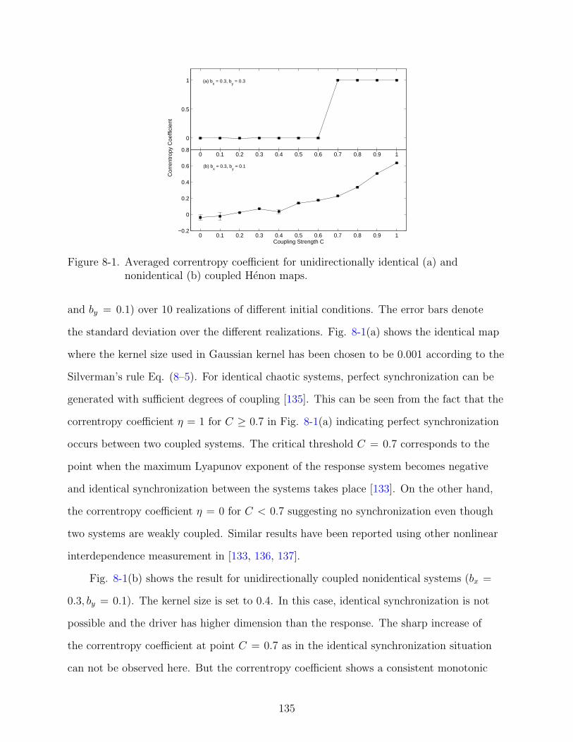
0 0.1 0.2 0.3 0.4 0.5 0.6 0.7 0.8 0.9 1−0.2
0
0.2
0.4
0.6
0.8
Coupling Strength C
0 0.1 0.2 0.3 0.4 0.5 0.6 0.7 0.8 0.9 1
0
0.5
1 (a) bx = 0.3, b
y = 0.3
(b) bx = 0.3, b
y = 0.1
Cor
rent
ropy
Coe
ffici
ent
Figure 8-1. Averaged correntropy coefficient for unidirectionally identical (a) andnonidentical (b) coupled Henon maps.
and by = 0.1) over 10 realizations of different initial conditions. The error bars denote
the standard deviation over the different realizations. Fig. 8-1(a) shows the identical map
where the kernel size used in Gaussian kernel has been chosen to be 0.001 according to the
Silverman’s rule Eq. (8–5). For identical chaotic systems, perfect synchronization can be
generated with sufficient degrees of coupling [135]. This can be seen from the fact that the
correntropy coefficient η = 1 for C ≥ 0.7 in Fig. 8-1(a) indicating perfect synchronization
occurs between two coupled systems. The critical threshold C = 0.7 corresponds to the
point when the maximum Lyapunov exponent of the response system becomes negative
and identical synchronization between the systems takes place [133]. On the other hand,
the correntropy coefficient η = 0 for C < 0.7 suggesting no synchronization even though
two systems are weakly coupled. Similar results have been reported using other nonlinear
interdependence measurement in [133, 136, 137].
Fig. 8-1(b) shows the result for unidirectionally coupled nonidentical systems (bx =
0.3, by = 0.1). The kernel size is set to 0.4. In this case, identical synchronization is not
possible and the driver has higher dimension than the response. The sharp increase of
the correntropy coefficient at point C = 0.7 as in the identical synchronization situation
can not be observed here. But the correntropy coefficient shows a consistent monotonic
135

0 0.2 0.4 0.6 0.8 1
0
0.05
0.1
(a)
0 0.2 0.4 0.6 0.8 1
0
0.01
0.02
(b)
0 0.2 0.4 0.6 0.8 1
0
0.05
0.1
(c)
Cor
rent
ropy
Coe
ffici
ent
0 0.2 0.4 0.6 0.8 1
0
0.02
0.04
(d)
0 0.2 0.4 0.6 0.8 1
0
0.02
0.04
0.06(e)
0 0.2 0.4 0.6 0.8 1
0
0.05
0.1
(f)
response + noise (SNR = 10dB)
driver + noise (SNR = 10dB)
response + noise (SNR = 10dB)
response + noise (SNR = 1dB)
driver + noise (SNR = 1dB)
driver + noise (SNR = 10dB) response + noise (SNR = 1dB) driver + noise (SNR = 1dB)
Coupling Strength C
Figure 8-2. Influence of different noise levels on correntropy coefficient.
increase with respect to coupling strength except for the region 0.1 < C < 0.3. The local
hump in this region can also be seen in [133, 134, 137]. It is suggested that the cause is
most likely due to the local minimum of the maximum Lyapunov exponent [133, 138] in
this region.
8.2.1.2 Robustness Against Measurement Noise
A good interdependence measure should be robust against noise. Next, we analyze
the robustness of correntropy coefficient when time series are contaminated with noise.
There are two types of noise in general: intrinsic noise and addictive measurement noise.
We only consider measurement noise here which does not perturb the inherent dynamics
of systems. Independent realizations of white noise are added to driver, response and both
systems separately. The signal-to-noise (SNR) ratio is set to be 10dB and 1dB respectively
to test the performance of correntropy coefficient at different noise intensity. 500 data
samples are used to calculated the correntropy coefficient, averaged over 20 realizations.
Fig. 8-2 plots the correntropy coefficient for unidirectionally coupled identical Henon
map (bx = by = 0.3) with white noise in response, driver and both systems. Kernel size
is chosen to be 0.04 for SNR = 10dB and 0.08 for SNR = 1dB respectively. Notice that
the correntropy coefficient curves with noise become less smooth than that of noise-free
136

0 0.2 0.4 0.6 0.8 1
0
0.04
0.08(a)
0 0.2 0.4 0.6 0.8 1−0.05
0
0.05
0.1
0.15
(b)
0 0.2 0.4 0.6 0.8 1
0
0.05
0.1(c)
Cor
rent
ropy
Coe
ffici
ent
0 0.2 0.4 0.6 0.8 1−0.05
0
0.05
0.1
0.15
(d)
0 0.2 0.4 0.6 0.8 1
0
0.02
0.04
0.06(e)
0 0.2 0.4 0.6 0.8 1
0
0.05
0.1
(f)
Coupling Strength C
response + noise (SNR = 10dB) response + noise (SNR = 1dB)
driver + noise (SNR = 10dB) driver + noise (SNR = 1dB)
response + noise (SNR = 10dB)
driver + noise (SNR = 10dB) response + noise (SNR = 1dB) driver + noise (SNR = 1dB)
Figure 8-3. Influence of different noise levels on correntropy coefficient.
one, but the sharp increase at C = 0.7 is still obvious for both noise intensities. When
noise level is high (SNR = 1dB), the correntropy coefficient curve is more zigzag than
that of 10dB case, however it can still detect increases in the coupling strength. The
figure also suggests that whether noise is added into driver, response or both system, the
performance of correntropy coefficient is very similar. Fig. 8-3 presents the results for
non-identical Henon map (bx = 0.3 and by = 0.1) with white noise in response, driver
and both systems. Kernel size is selected to 0.05 for SNR = 10dB and 0.2 for SNR = 1dB
respectively. The values of the correntropy coefficients at different coupling strength are
averaged over 20 independent realizations. In both levels of noise case, the correntropy
coefficients consistently increase with respect to coupling strength. Also the effect of noise
in response, driver or both systems does not make big differences. Notice that the local
hump around the region 0.2 < C < 0.4 is still observable for all cases. These results show
that the correntropy coefficient is fairly robust even in the case of considerably noisy data.
8.2.1.3 Sensitivity to Time-dependent Dynamical Changes
Next we test how sensitive the correntropy coefficient is to time dependent sudden
change in the dynamics of interacting systems due to coupling strength. In experiment,
change in coupling strength can cause sudden change in the dynamics of interacting
137

50 150 250 350−0.1
0
0.1
0.3
50 150 250 350−0.2
0
0.2
0.4
0.6
0.8
1
Cor
rent
ropy
Coe
ffici
ent
(a) bx = 0.3, b
y = 0.3
(b) bx = 0.3, b
y = 0.1
Time t
Figure 8-4. Time dependent of correntropy coefficient.
systems, which basically generates non-stationarity in time series. To study such transient
dynamical phenomenon, both identical (bx = by = 0.3) and non-identical (bx = 0.3 and
by = 0.1) Henon maps are considered here. Dynamical systems are coupled only during
a single epoch and otherwise uncoupled for both cases [134, 137]. We set the coupling
strength C = 0 for n ≤ 10150 and n ≥ 10250 and C = 0.8 for 10150 < n < 10250.
Only 400 data samples are plotted after the first 10000 data are discarded as transient.
The sliding window used to compute the correntropy coefficient is chosen to contain
8 data. Kernel size is set to 0.2 for identical map and 0.3 for non-identical map. The
results are averaged over 20 independent realizations of different initial conditions ranging
0 to 1. Fig. 8-4 plots the correntropy coefficient curves for identical and non-identical
maps. In uncoupled regions, η fluctuates around 0.01 baseline for identical map and
0.001 for non-identical map. A sharp and clear increase occurs at t = 150 when 0.8
coupling strength between systems X and Y is introduced, and there is a sharp and
clear decrease in η falling off back to the baseline level when coupling strength between
two systems reduces to zero at t = 250. The interval where η is noticeably higher than
the baseline level matches nicely to the coupling interval. This phenomenon is observed
both in identical and non-identical Henon maps. Therefore, the correntropy coefficient
138

00.2
0.40.6
0.81
10−5
10−3
10−1
101
−0.2
0
0.2
0.4
0.6
0.8
1
1.2
coupling strength C
corr
entr
opy
coef
ficie
nt
kernel width σ
Figure 8-5. Effect of different kernel width on correntropy coefficient for unidirectionallycoupled identical Henon maps.
is potentially able to detect sudden change in the coupling between two interacting
dynamical systems with a high temporal resolution, which makes this measure suitable for
non-stationary data sets.
8.2.1.4 Effect of Kernel Width
We have discussed the importance of the kernel width in the performance of the
correntropy coefficient because it is a parametric measure in previous section. Here we
demonstrate this on unidirectionally coupled identical and non-identical Henon maps. Fig.
8-5 shows the correntropy coefficient curves of different kernel width for unidirectionally
coupled identical Henon map. When the kernel width is chosen too large, σ = 0.1, 0.5,
1, in this case, correntropy coefficient produces erroneous results in the unsynchronized
region 0 < C < 0.7. The results for non-identical Henon map are presented in Fig. 8-6.
It can be seen that if kernel width is too small, the increase of the correntropy coefficient
with respect to the coupling strength is not as obvious as those of suitable kernel width (σ
= 0.4 here). While the kernel width is too larger, the results of the correntropy coefficient
approach to those of conventional correlation coefficient. In both figures, we see that the
correntropy coefficients can either increase or decrease as the kernel width increases. These
observations are consistent with our theoretical analysis in previous section.
139

00.2
0.40.6
0.81
0
1
2
3
4−0.2
0
0.2
0.4
0.6
0.8
1
1.2
coupling strength Ckernel width σ
corr
entr
opy
coef
ficie
nt
Figure 8-6. Effect of different kernel width on correntropy coefficient for unidirectionallycoupled non-identical Henon maps.
8.2.1.5 Ability to Quantify Nonlinear Coupling
To demonstrate that correntropy coefficient η is able to detect the nonlinear coupling
between systems X and Y, we first compare our measure with the conventional correlation
coefficient and one of the well-known nonlinear synchronization measure, similarity
index in [133], on identical Henon maps. Fig. 8-7 shows the correlation coefficient, the
correntropy coefficient and the similarity index as functions of coupling strength C.
The correntropy coefficient generates exactly the same result as the similarity index.
On the other hand the conventional correlation coefficient performs erratically in the
unsynchronized region C < 0.7. This clearly demonstrates that the correntropy coefficient
outperforms the correlation coefficient in characterization of nonlinear coupling between
two dynamical systems. Compared to the similarity index, the correntropy coefficient has
the advantage of avoiding estimating embedding dimension, choosing nearest neighborhood
and other problems associated with state space embedding method [133, 139]. The
computational complexity of the correntropy coefficient is still manageable, and the kernel
size is easy to estimate.
We also use multivariate surrogate data to further investigate that the correntropy
coefficient is sensitive to nonlinear coupling. Prichard et al. introduced surrogate method
140

0 0.1 0.2 0.3 0.4 0.5 0.6 0.7 0.8 0.9 1
0
0.5
1
Coupling Strength C
0
0.5
1
0
0.5
1Correlation coefficient
Correntropy coefficient
Similarity Index
Figure 8-7. Comparison of correlation coefficient, correntropy coefficient and similarityindex.
in [140]. This method has been applied to detect nonlinear structure in time series.
Basically, to generate multivariate surrogate data, first the Fourier transform is applied to
each of time series, then a common random number is added to each of the phases and an
inverse Fourier transform is applied. The resulting time series have identical power spectra
and cross power spectra as the original time series, but any nonlinear coupling among the
time series has been destroyed. In simulation, we use TISEAN package [141] to generate
19 realizations of the surrogate data for the time series x1(t) in Eq. (8–1) and y1(t) in Eq.
(8–3) for each different coupling strength for the unidirectionally coupled non-identical
Henon map. Then we compute the correntropy coefficient for both the original and the
surrogate data with respect to different coupling strength. Fig. 8-8 plots the correntropy
coefficient curve for the original data and the mean value of 19 correntropy coefficients
for the surrogate data with the corresponding maximal and minimal values as error bars.
To quantify the significance level, we calculate the Z-Score as Z =|vorig−µsurr|
σsurrwhere vorig
is the correntropy coefficient value for the original data, µsurr and σsurr are the mean
and the standard deviation for the surrogate data respectively. Table 8-1 presents the
Z-Score values for different coupling strength. With the exception of C = 0.2 and 0.4,
the Z-Score values are significantly larger than 1.96 which means the nonlinear coupling
141

0 0.1 0.2 0.3 0.4 0.5 0.6 0.7 0.8 0.9 1−0.1
0
0.1
0.2
0.3
0.4
0.5
0.6
0.7
0.8Original DataSurrogate Data
Coupling Strength C
Cor
rent
ropy
Coe
ffici
ent
Figure 8-8. Comparison of the correntropy coefficient for the original data and thesurrogate data for unidirectionally coupled non-identical Henon map.
has been detected with a probability p < 0.05. These results clearly demonstrates that
the correntropy coefficient is sensitive to the nonlinearity of the dependence between two
coupled systems.
8.2.2 EEG Signals
In the second experiment, we applied the correntropy coefficient to real EEG signals.
The electrical potentials on the surface of the scalp of a human subject were measured and
recorded with the NeuroScan EEG system (NeuroScan Inc., Compumedics, Abbotsford,
Australia). A 64-channel cap was used with electrode locations according to the extended
international 10/20 system and with a linked-earlobe reference. Horizontal and vertical
electrooculogram (HEOG and VEOG) signals were also recorded for artifact rejection
using two sets of bipolar electrodes. The data sampling rate was fixed at 1000Hz and the
online band-pass filter range was set to be maximally wide between 0.05Hz and 200Hz.
Subjects were presented repeatedly (200 times) with uni-modal auditory and visual
stimuli delivered in the central visual and auditory spaces simultaneously and with the
same strength to the left/right eyes and ears, as well as with simultaneous cross-modal
combinations. For the purpose of this study, only the uni-modal data was used. The visual
142

Table 8-1. Z-score for the surrogate data
C 0 0.1 0.2 0.3 0.4 0.5 0.6 0.7 0.8 0.9 1Z Score 6.943 4.472 1.622 4.585 0.773 7.658 9.908 16.699 12.268 22.588 19.895
stimuli consisted of 5x5 black and white checkerboards presented for 10ms, while the
auditory stimuli were 2000Hz tones with durations of 30ms. The time interval between the
stimuli in any of the experimental conditions was random between 1500ms and 2000ms.
Following standard eye-movement artifact rejection procedures and segmentation into
single epochs with alignment at the onset of the stimuli, all artifact-free epochs were
averaged and normalized to zero mean and unit variance and low-pass filtered at 0-40Hz
for further analysis. We then applied the correntropy coefficient to the averaged data to
quantify the bilateral synchronization or couplings among the corresponding sensory areas
of the brain. In order to test whether the correntropy coefficient was able to detect any
nonlinear couplings in the EEG signals, the results were compared to the conventional
correlation coefficient. A window size of 20ms data is used to calculate both measures
corresponding to the duration of a single dipole activation in the cortex [142]. The kernel
width σ in Gaussian kernel used in correntropy coefficient was chosen to be 0.4.
Fig. 8-9 (a) and (b) show plots of the correlation and correntropy coefficients for
the auditory areas of the brain as a function of time after the subject was exposed only
to the audio stimuli. Several bilaterally-symmetrical pairs of electrodes were selected
in the vicinity of the auditory cortex , so that both measures were computed for pairs
FC5-FC6, FC3-FC4, C5-C6, C3-C4, CP5-CP6, CP3-CP4. As shown in Fig. 8-9 (a)
and (b), there are two distinct time intervals 0-270ms and 270-450ms in the auditory
response. Both correlation and correntropy coefficients drop at 270ms. This suggests that
both measures are able to detect the changes in inter-hemispheric synchronization of the
auditory regions. However, as the electrodes are chosen in different locations away from
the auditory cortex, it is expected that during the synchronization phase (0-270ms) the
synchronization measures for different pairs should be different. Fig. 8-9 (a) shows that
143

0 50 100 150 200 250 300 350 400 450
0
0.5
1
Time/ms
Co
rre
ntr
op
y C
oe
ffic
ien
t
250 450
0
0.5
1
Co
rre
latio
n C
oe
ffic
ien
t
FC5−FC6FC3−FC4C5−C6C3−C4CP5−CP6CP3−CP4
(a)
(b)
Figure 8-9. Comparison of correlation coefficient and correntropy coefficient insynchronization detection among auditory cortex for audio stimuli EEG signal.
the correlation coefficients for all 6 pairs are grouped together and are unable to detect
the difference in activation, while Fig. 8-9 (b) suggests that the correntropy coefficient can
differentiate successfully the synchronization strength among different areas of the cortex
above the left and right auditory regions. Notably, as expected from previous studies,
pairs FC5-FC6 and FC3-FC4 exhibit stronger synchronization strength than the others,
while most posterior pairs CP5-CP6 and C5-C6 have weaker synchronization strength.
Also the synchronization patterns reveal lateral similarity in time for the pairs FC5-FC6
and FC3-FC4, for CP5-CP6 and C5-C6, and for CP3-CP4 and C3-C4. Furthermore the
correntropy coefficients for pairs C5-C6, C3-C4 and CP3-CP4 peak simultaneously at 90ms
which corresponds to the first mean global field power (MGFP) peak of the EEG signal.
144

0 100 200 300 400 500 600
0
0.5
1
Time/ms
300 600
0
0.5
1
O1−O2PO7−PO8PO5−PO6P7−P8P5−P6P3−P4
Co
rre
latio
n C
oe
ffic
ien
tC
orr
en
tro
py C
oe
ffic
ien
t
(a)
(b)
Figure 8-10. Comparison of correlation coefficient and correntropy coefficient incharacterization of synchronization among occipital cortex for visual stimulusEEG signal.
These differences indicate that the correntropy coefficient is more sensitive and is able to
extract more information as a synchronization measure than the conventional correlation
coefficient.
We also compared both measures when applied to the visual cortical areas. The
measures are presented in Fig. 8-10 as a function of time when the subject is exposed
only to visual stimuli. Again, a window size of 20ms data is used to compute both
the correlation and the correntropy coefficients, and the kernel width σ is again set to
0.4 as in the previous case. We also chose bilaterally symmetrical pairs of electrodes
O1-O2, PO7-PO8, PO5-PO6, P7-P8, P5-P6 and P3-P4. In Fig. 8-10 (b) the correntropy
coefficients for all pairs except for O1-O2 show similar synchronization patterns. The
145

correntropy coefficient increases at first, then reaches a peak around 275ms, after which
it drops to lower levels. The maximum values of the correntropy coefficients around
275ms correspond to the peak P1 in the visual evoked potential [143]. As expected
the synchronization between occipital channels O1 and O2 has the maximum strength
and stays high until it decreases around 350ms. Thus the correntropy coefficient shows
that the extra-striate visual networks become increasingly recruited and synchronized
until about 275ms after the stimulus onset, while the primary visual cortex is highly
synchronous for a longer period of time, until about 350ms after onset. The channels pair
P7 and P8 exhibits the weakest synchronization strength since it is located the farthest
away from the primary visual cortex compared to other electrode pairs. On the other
hand, the correlation coefficients for most channel pairs group together and display the
same level of synchronization until its sharp decrease at around 500ms (except for P7-P8).
The synchronization between P7 and P8 has irregular patterns with a local minimum
around 200ms. This comparison clearly demonstrates that also in this case the correntropy
coefficient measure outperforms the correlation coefficient in the quantification of the EEG
signal coupling between the bilateral occipital regions of the brain in response to visual
stimuli.
8.3 Discussions
In this section, we explore more details about the correntropy coefficient both in
theoretical analysis and practical implementation such as the geometrical interpretation,
connections to information theory, the important role of the kernel size, and the scaling
factor of time series.
8.3.1 Kernel Width
The variance of the Gaussian kernel function is normally called kernel width or kernel
size. The kernel size should be considered a scale parameter controlling the metric in the
projected space. From the geometrical perspective, the kernel size decides the length of
each of the nonlinearly transformed vectors and the angle between them in the RKHS
146

HU because ‖Ψ(x)‖ =√
κ(0)− 1N2
∑Ni=1
∑Nj=1 κ(xi, xj). It can be easily seen that the
vector length monotonically decreases as the kernel width increases, while the centered
crosscorrentropy exhibits more complex pattern since it also depends on the nature of
the relationship between two random variables. The kernel width controls the ability of
the centered correntropy to capture the nonlinear couplings intrinsic in the signals. If
the kernel width is too large, the correntropy coefficient loses the ability to detect the
nonlinearity and approaches the conventional correlation coefficient; when the kernel
width is too small, the nonlinear transformations Φ in Eq. (4–3) and Ψ in Eq. (4–29)
cannot interpolate between data points. This can also be verified to apply the Taylor
series expansion to the Gaussian kernel where the kernel width appears as the weighting
parameter in both second and higher order moments. The effect of the kernel size on
different order moments is scaled by the power up to 2k where k is the moment order.
When the kernel size is too large, the contribution of higher order statistics decays rapidly
and the centered crosscorrentropy approaches the conventional crosscovariance function;
on the other hand, when the kernel size is too small, the effect of higher order moments
overweighs the second order one. An appropriate kernel size should maintain the balance
of second order and higher order statistics of the signal.
Therefore a good choice of the kernel parameter is crucial for obtaining the good
performance of the proposed method. There are two ways of handling the selection of
kernel size. One is to seek an optimal kernel size. The cross-validation has been one of
the mostly used methods in machine learning field to choose an appropriate kernel width.
Other approaches include the Silverman’s rule of thumb which is given by [120]:
σ = 0.9AN−1/5, (8–5)
where A is the smaller value between standard deviation of data samples and data
interquartile range scaled by 1.34, and N is the number of data samples. The Silverman’s
rule is easy to use to choose a good kernel size, hence we will set the kernel width
147

according to Eq. (8–5) throughout the paper. Alternatively, the kernel size can be
thought as a scale parameter that provides different looks to the dependence among the
variables. Just like in wavelets, the kernel size is able to analyze the dependencies at
different resolutions. Since many real world signals are very complex, this multi-resolution
analysis may elucidate better the relationships.
8.3.2 Scaling Effect
Because the nonlinear transformations Φ in Eq. (4–3) and Ψ in Eq. (4–29) are
nonlinear, any scaling of the original random variables results in different performance
of the correntropy coefficient. Unlike the conventional correlation coefficient which
is insensitive the amplitude scaling of the signals and only measures the similarity of
the signals through the time, the correntropy coefficient measures both the time and
amplitude similarities between two signals. Therefore, in certain applications, it is vital
to normalize both signals before applying the correntropy coefficient. For example, the
amplitudes of EEG signals are highly dependent on the different electrode impedances. It
is important to normalize all channels of EEG signals to the same dynamical range.
8.4 Conclusion
In this chapter, we apply the correntropy coefficient as a novel nonlinear interdependence
measure. Due to a positive definite kernel function, the correntropy coefficient implicitly
maps the original random variables or time series into an infinite dimensional reproducing
kernel Hilbert space which is uniquely induced by the centered crosscorrentropy function
and essentially computes the cosine of the angle between the two transformed vectors.
Orthogonality in RKHS HU corresponds to independence between original random
variables. Comparisons between the correntropy coefficient and the conventional
correlation coefficient on simulated two unidirectionally coupled Henon maps time
series and EEG signals collected from sensory tasks clearly illustrate that the correntropy
coefficient is able to extract more information than the correlation coefficient in quantification
of synchronization between interacting dynamical systems.
148

CHAPTER 9CONCLUSIONS AND FUTURE WORK
9.1 Conclusions
In this dissertation, we have analyzed the recently proposed correntropy function [65]
and presented a new centered correntropy function from Time-domain and frequency-domain
approaches. It is demonstrated that correntropy and centered correntropy functions not
only capture the time and space structures of signals, but also partially characterize the
high order statistical information and nonlinearity intrinsic to signals. Correntropy and
centered correntropy functions have rich geometrical structures. Correntropy is positive
definite and centered correntropy is non-negative definite, hence by Moore-Aronszajn
theorem they uniquely induce reproducing kernel Hilbert spaces. Correntropy and
centered correntropy functions combine the data dependent expectation operator and data
independent kernels to form another data dependent operator. One perspective to work
with correntropy and centered correntropy functions is to treat them as “generalized”
correlation and covariance functions on nonlinearly transformed random signals via the
data independent kernel functions. Those nonlinearly transformed signals appear on the
sphere in the RKHS induced by the kernel functions if isotropic kernel functions are used.
The other perspective is to directly work with the RKHS induced by the correntropy
and centered correntropy functions directly. Now the nonlinearly transformed signals
in the RKHS is no longer stochastic but rather deterministic. The RKHS induced by
the correntropy and centered correntropy functions includes the expectation operator
as embedded vectors. The two views further our understandings of correntropy and
centered correntropy functions in geometrical perspective. The two reproducing kernel
Hilbert spaces induced by kernel functions and correntropy functions respectively represent
stochastic and deterministic functional analysis.
The correntropy dependence measure is proposed based on the correntropy coefficient
as a novel statistical dependence measure. The new measure satisfies all the fundamental
149

desirable properties postulated by Renyi. We apply the correntropy concept in pitch
determination, and nonlinear component analysis. The correntropy coefficient is also
employed as a novel similarity measure to quantify the inder-dependencies of multi-channel
signals.
9.2 Future work
As we have provide a new methodology to explicitly construct a reproducing kernel
Hilbert space induced by the data independent kernel functions, we would like to apply
the same methodology to construct the RKHS induced by the data dependent correntropy
function directly. This shall allow us to analyze the functional basis that consists of the
RKHS. Moreover, if we can have an explicit expression for those functionals, then we can
develop algorithms that are not restricted to the inner product. We have only test our
correntropy PCA algorithms on artificial data sets. It is desired to apply the algorithms to
real data set. Some of the future work might includes
1. applying the parametric correntropy coefficient in detecting nonlinear coupling for
EEG signal,
2. investigating the relationship between the higher order statistics and correntropy,
3. applying correntropy pitch determination algorithm in multiple pitches tracking.
150

LIST OF REFERENCES
[1] N. Aronszajn, “The theory of reproducing kernels and their applications,” Cam-bridge Philosophy Soceity Proceedings, vol. 39, pp. 133–153, 1943.
[2] N. Aronszajn, “Theory of reproducing kernels,” Transactions of the AmericanMathemathical Society, vol. 68, no. 3, pp. 337–404, 1950.
[3] A. Povzner, “On a class of hilbert function spaces,” Dokl. Akad. Nauk. SSSR, vol.68, pp. 817–820, 1949.
[4] A. Povzner, “On some applications of a class of hilbert function spaces,” Dokl.Akad. Nauk. SSSR, vol. 74, pp. 13–16, 1950.
[5] M. G. Krein, “Hermitian-positive kernels on homogeneous spaces,” AmericanMathematical Society Translation, vol. 2, no. 34, pp. 69–164, 1963.
[6] E. Hille, “Introduction to general theory of reproducing kernels,” Rocky MountainJournal of Mathematics, vol. 2, pp. 321–368, 1972.
[7] H. Meschkowski, Hilbert Spaces with Kernel Function, Springer-Verlag, Berlin, 1962.
[8] H. S. Shapiro, Topics in Appproximation Theory, Springer-Verlag, Berlin, 1971.
[9] S. Saitoh, Theory of Reproducing Kernels and its Applications, Pitman researchnotes in mathematics series. Longman Scientific & Technical, Essex,UK, 1988.
[10] P. J. Davis, Interpolation and Approximation, Dover, New York, 1975.
[11] S. Bergman, The Kernel Function and Conformal Mapping, American MathematicalSociety, New York, 1950.
[12] L. Schwartz, “Hilbert subspaces of topological vector spaces and associated kernels,”Journal of Analysis Mathematics, vol. 13, pp. 115–256, 1964.
[13] J. Mercer, “Functions of positive and negative type, and their connection with thetheory of integral equations,” Philosophical Transactions of the Royal Society ofLondon, vol. 209, pp. 415–446, 1909.
[14] E. H. Moore, “On properly positive hermitian matrices,” Bulletin of the AmericanMathematical Society, vol. 23, no. 59, pp. 66–67, 1916.
[15] Salomon Bochner, “Hilbert distances and positive definite functions,” The Annals ofMathematics, vol. 42, no. 3, pp. 647–656, July 1941.
[16] I. J. Schoenberg, “Metric spaces and positive definite functions,” Transactions of theAmerican Mathemathical Society, vol. 44, pp. 522–536, 1938.
[17] I. J. Schoenberg, “Positive definite functions on spheres,” Duke Math. J., vol. 9, pp.96–108, 1942.
151

[18] J. Stewart, “Positive definite functions and generalizations, an historical survey,”Rocky Mountain Journal of Mathematics, vol. 6, no. 3, pp. 409–434, September 1976.
[19] D. Alpay, Ed., Reproducing Kernel Spaces and Applications, Birkhauser Verlag,Germany, 2003.
[20] U. Grenander, Abstract Inference, John Wiley & Sons, New York, 1981.
[21] E. Kreyszig, Introductory Functional Analysis with Applications, John Wiley & Sons,New York, 1978.
[22] A. N. Kolmogorov, “Stationary sequences in Hilbert space,” Bull. Math. Univ.Moscow, vol. 2, no. 6, 1941.
[23] M. Loeve, “Stochastic prcesses and brownina motion,” in Second Order RandomFuntions, P. Levy, Ed., p. 365. Cauthier-Villars, Paris, 1948.
[24] M. Loeve, Probability Theory II, Springer-Verlag, Berlin, 4th edition, 1978.
[25] E. Parzen, “Statistical inference on time series by Hilbert space methods,” TechnicalReport 23, Statistics Department, Stanford University, 1959.
[26] E. Parzen, “Statistical inference on time series by RKHS methods,” in Proc.12th Biennial Seminar Canadian Mathematical Congress, R. Pyke, Ed., Montreal,Canada, 1970, pp. 1–37.
[27] E. Parzen, “An approach to time series analysis,” The Annals of MathematicalStatistics, vol. 32, no. 4, pp. 951–989, December 1961.
[28] E. Parzen, “Extraction and detection problems and reproducing kernel Hilbertspaces,” SIAM Journal on Control, vol. 1, pp. 35–62, 1962.
[29] E. Parzen, Time Series Analysis Papers, Holden-Day, San Francisco, CA, 1967.
[30] J. Hajek, “On linear statistical problems in stochastic processes,” CzechoslovakMathematical Journal, vol. 12, pp. 404–444, 1962.
[31] T. Kailath, “RKHS approach to detection and estimation problems–part I:Deterministic signals in gaussian noise,” IEEE Transactions on InformationTheory, vol. IT-17, no. 5, pp. 530–549, September 1971.
[32] T. Kailath and H. Weinert, “An RKHS approach to detection and estimationproblems–part II: Gaussian signal detection,” IEEE Transactions on InformationTheory, vol. IT-21, no. 1, pp. 15–23, January 1975.
[33] T. Kailath and D. Duttweiler, “An RKHS approach to detection and estimationproblems–part III: Generalized innovations representations and a likelihood-ratioformula,” IEEE Transactions on Information Theory, vol. IT-18, no. 6, pp. 730–745,November 1972.
152

[34] D. Duttweiler and T. Kailath, “RKHS approach to detection and estimationproblems–part IV: Non-gaussian detection,” IEEE Transactions on InformationTheory, vol. IT-19, no. 1, pp. 19–28, January 1973.
[35] D. Duttweiler and T. Kailath, “RKHS approach to detection and estimationproblems–part V: Parameter estimation,” IEEE Transactions on InformationTheory, vol. IT-19, no. 1, pp. 29–37, January 1973.
[36] T. Hida and N. Ikeda, “Analysis on hilbert space with reproducing kernel arisingfrom multiple wiener integral,” in Proc. 5th Berkely Symp. on MathematicalStatistics and Probability, L. LeCam and J. Neyman, Eds., 1967, vol. 2, pp. 117–143.
[37] G. Kallianpur, “Advances in probability and related topics,” in The Role ofReproducing Kernel Hilbert Spaces in the Study of Gaussian Processes, P. Ney, Ed.,vol. 2, pp. 49–83. Marcel Dekker, New York, 1970.
[38] T. Hida, “Canonical representations of gaussian processes and their applications,”Kyoto Univ. Coll. Sci. Mem., vol. A33, pp. 109–155, 1960.
[39] G. M. Molchan, “On some problems concerning brownian motion in levy’s sense,”Theory of Probability And Its Applications, vol. 12, pp. 682–690, 1967.
[40] L. Pitt, “A markov property for gaussian processes with a multidimensionalparameter,” Archive for Rational Mechanics and Analysis, vol. 43, pp. 367–391,1971.
[41] H. L. Weinert, “Statistical methods in optimal curve fitting,” Communications inStatistics, vol. B7, no. 4, pp. 417–435, 1978.
[42] C. De Boor and R. E. Lynch, “On splines and their minimum properties,” Journalof Mathematics and Mechanics, vol. 15, pp. 953–969, 1966.
[43] L. L. Schumaker, “Fitting surfaces to scattered data,” in Approximation Theory II,G.G. Lorentz, C. K. Chui, and L.L. Schumaker, Eds., pp. 203–268. Academic Press,New York, 1976.
[44] G. Wahba, Spline Models for Observational Data, vol. 49, SIAM, Philadelphia, PA,1990.
[45] Rui J.P. DeFigueiredo, “A generalized fock space framework for nonlinear systemand signal analysis,” IEEE Transactions on Circuits and Systems, vol. CAS-30, no.9, pp. 637–647, September 1983.
[46] V. N. Vapnik, The Nature Statistical Learning Theory, Springer, New York, 1999.
[47] V. N. Vapnik, Statistical Learning Theory, John Wiley & Sons, New York, 1998.
[48] F. Rosenblatt, “The perceptron: A probabilistic model for information storage andorganization in the brain,” Psychological Review, vol. 65, no. 6, pp. 386–408, 1958.
153

[49] B. Scholkopf and A. Smola, Learning with kernels, MIT Press, Cambridge, MA,2002.
[50] B. Scholkopf, A. Smola, and K.-R. Muller, “Nonlinear component analysis as akernel eigenvalue problem,” Neural Computation, vol. 10, pp. 1299–1319, 1998.
[51] J. Weston B. Scholkopf S. Mika, G. Ratsch and K.-R. Muller, “Fisher discriminantanalysis with kernels,” in Proc. Neural Networks for Signal Processing IX, NewJersey, 1999, vol. 2, pp. 41–48.
[52] F. R. Bach and M. I. Jordan, “Kernel independent component analysis,” Journal ofMachine Learning Research, vol. 3, pp. 1–48, 2002.
[53] Thomas M. Cover, “Geometrical and statistical properties of systems of linearinequalities with applications in pattern recognition,” IEEE Transactions onElectronic Computers, vol. EC-14, no. 3, pp. 326–334, June 1965.
[54] T. Evgeniou, T. Poggio, M. Pontil, and A. Verri, “Regularization and statisticallearning theory for data analysis,” Computational Statistics and Data Analysis, vol.38, pp. 421–432, 2002.
[55] J. C. Principe, D. Xu, and J. W. Fisher, “Information theoretic learning,” inUnsupervised Adaptive Filtering, S. Haykin, Ed., pp. 265–319. John Wiley & Sons,2000.
[56] K. E. Hild, D. Erdogmus, and J. C. Principe, “Blind source separation using Renyi’smutual informaiton,” IEEE Signal Processing Letter, vol. 8, no. 6, pp. 174–176, 2001.
[57] D. Erdogmus and J. C. Principe, “Generalized information potential criterion foradaptive system training,” IEEE Transactions on Neural Networks, vol. 13, no. 5,pp. 1035–1044, 2002.
[58] A. Renyi, “On measures of entropy and information,” in Selected paper of A. Renyi,vol. 2, pp. 565–580. Akademiai Kiado, Budapest, Hungary, 1976.
[59] D. Erdogmus and J. C. Principe, “An error-entropy minimization algorithm forsupervised training of nonlinear adaptive systems,” IEEE Transactions on SignalProcessing, vol. 50, no. 7, pp. 1780–1786, July 2002.
[60] E. Parzen, “On estimation of a probability density function and mode,” The Annalsof Mathematical Statistics, vol. 33, no. 3, pp. 1065–1076, September 1962.
[61] M. G. Genton, “Class of kernels for machine learning: A statistics perspective,”Journal of Machine Learning Research, vol. 2, pp. 299–312, 2001.
[62] S. Kullback and R. A. Leibler, “On information and sufficiency,” The Annals ofMathematical Statistics, vol. 22, no. 1, pp. 79–86, 1951.
154

[63] D. Xu, J. C. Principe, J. W. Fisher, and H. C. Wu, “A novel measure forindependent component analysis,” in Proceedings of the IEEE InternationalConference on Acoustics, Speech, and Signal Processing(ICASSP), 1998, vol. 2, pp.12–15.
[64] R. Jenssen, D. Erdogmus, J. C. Principe, and T. Eltoft, “The laplacian PDFdistance: A cost function for clustering in a kernel feature space,” in Advancesin Neural Information Processing Systems (NIPS). 2004, pp. 625–632, MIT Press,Cambridge.
[65] I. Santamaria, P. Pokharel, and J. C. Principe, “Generalized correlation function:Definition, properties, and application to blind equalization,” IEEE Transactions onSignal Processing, vol. 54, no. 6, pp. 2187–2197, 2006.
[66] P. P. Pokharel, R. Agrawal, and J. C. Principe, “Correntropy based matchedfiltering,” in Proc. Machine Learning for Signal Processing, Mystic, USA, 2005.
[67] K.-H. Jeong and J. C. Principe, “The correntropy MACE filter for imagerecognition,” in Proceedings of the International Workshop On Machine Learn-ing for Signal Processing(MLSP), Maynooth, Ireland, 2006, pp. 9–14.
[68] P. P. Pokharel, J. Xu, D. Erdogmus, and J. C. Principe, “A closed form solutionfor a nonlinear Wiener filter,” in Proceedings of the IEEE International Conferenceon Acoustics, Speech, and Signal Processing(ICASSP), Toulouse, France, May 2006,vol. 3, pp. 720–723.
[69] S.-I. Amari and H. Nagaoka, Methods of Information Geometry, AMS and OxfordUniversity Press, Providence, RI, 2000.
[70] B. Pistone and C. Sempi, “An infinite-dimensional geometric structure on the spaceof all probability measures equivalent to a given one,” The Annals of Statistics, vol.23, no. 5, pp. 1543–1561, 1995.
[71] C. R. Rao, “Information and accuracy attainable in the estimation of statisticalparameters,” Bulletin of the Calcutta Mathematical Society, vol. 37, pp. 81–91, 1945.
[72] T. Jebara, R. Kondor, and A. Howard, “Probability product kernels,” Journal ofMachine Learning Research, vol. 5, pp. 819–844, 2004.
[73] T. Jebara and R. Kondor, “Bhattarcharyya and expected likelihood kernels,” inProceedings of Annual Conference on Learning Theory, Washington D.C., 2003.
[74] M. B. Pursley, Random Processes in Linear Systems, Prentice Hall, New Jersey,2002.
[75] L. Ljung, System Identification: Theory for the User, Prentice-Hall, EnglewoodCliffs, NJ, 1987.
155

[76] Rui J.P. DeFigueiredo and Y. Hu, “Volterra equations and applications,” inOn Nonlinear Filtering of Non-Gaussian Processes Through Volterra Series,C. Corduneanu and I.W. Sandberg, Eds., pp. 197–202. Gordon and Breach Science,2002.
[77] R.F. Engle, “Autoregressive conditional heteroscedasticity with estimates of thevariance of united kingdom inflation,” Econometrica, vol. 50, pp. 987–1007, 1982.
[78] A. Rakotomamonjy and S. Canu, “Frames, reproducing kernels, regularization andlearning,” Journal of Machine Learning Research, vol. 6, pp. 1485–1515, 2005.
[79] V. Fock, “Konfigurationsraum und zweite quantelung,” Z. Phys., vol. 75, pp.622–647, 1932.
[80] D. Drouet Mari and S. Kotz, Correlation and Depedence, Imperieal College Press,London, 2001.
[81] J. Dauxiois and G. M. Nkiet, “Nonlinear canonical analysis and independence tests,”The Annals of Statistics, vol. 26, no. 4, pp. 1254–1278, 1998.
[82] C. B. Bell, “Mutual information and maximal correlation as measures ofdependence,” The Annals of Mathematical Statistics, vol. 33, no. 2, pp. 587–595,1962.
[83] T. Cover and J. Thomas, Elements of Information Theory, Wiley, New York, 1991.
[84] A. C. Micheas and K. Zografos, “Measureing stochastic dependence usingϕ-divergence,” Journal of Multivariate Analysis, vol. 97, pp. 765–784, 2006.
[85] S. D. Silvey, “On a measure of association,” The Annals of Mathematical Statistics,vol. 35, no. 3, pp. 1157–1166, 1964.
[86] H. Joe, “Relative entropy measures of multivariate dependence,” Journal of theAmerican Statistical Association, vol. 84, no. 405, pp. 157–164, 1989.
[87] C. W. Granger, E. Maasoumi, and J. Racine, “A dependence metric for possiblynonlinear processes,” Journal of Time Series Analysis, vol. 25, no. 5, pp. 649–669,2004.
[88] P. L. Lai and C. Fyfe, “Kernel and nonlinear canonical correlation analysis,”International Journal of Neural Systems, vol. 10, no. 5, pp. 365–377, 2000.
[89] A. Gretton, R. Herbrich, A. Smola, O. Bousquet, and B. Scholkopf, “Kernel methodsfor measuring independence,” Journal of Machine Learning Research, vol. 6, pp.2075–2129, 2005.
[90] H. Suetani, Y. Iba, and K. Aihara, “Detecting generalized synchronization betweenchatoic signals: A kernel-based approach,” Journal of Physics A: Mathematical andGeneral, vol. 39, pp. 10723–10742, 2006.
156

[91] A. Renyi, “On measure of dependence,” Acta Mathematica Academiae ScientiarumHungaricae, vol. 10, pp. 441–451, 1959.
[92] K. I. Diamantaras and S. Y. Kung, Principal Component Neural Networks: Theoryand Applications, John Wiley & Sons, New York, 1996.
[93] I.T. Jolliffe, Principal Component Analysis, Springer, New York, 2nd edition, 2002.
[94] T. Hastie and W. Stuetzle, “Principle curves,” Journal of the American StatisticalAssociation, vol. 84, no. 406, pp. 502–516, June 1989.
[95] M. A. Kramer, “Nonlinear principal component analysis using autoassociative neuralnetworks,” AIchE Journal, vol. 37, pp. 233–243, 1991.
[96] W. J. Hess, Pitch Determination of Speech Signals, Springer, New York, 1993.
[97] M. J. Ross, H. L. Shaffer, A. Cohen, R. Freudberg, and H. J. Manley, “Averagemagnitude difference function pitch extractor,” IEEE Transactions on Acoustics,Speech, and Signal Processing, vol. ASSP-22, no. 5, pp. 353–362, October 1974.
[98] A. de Cheveigne, “Cancellation model of pitch perception,” The Journal of theAcoustical Society of America, vol. 103, no. 3, pp. 1261–1271, March 1998.
[99] T. Shimarura and H. Kobayashi, “Weighted autocorrelation for pitch extraction ofnoisy speech,” IEEE Transactions on Speech and Audio Processing, vol. 9, no. 7, pp.727–730, October 2001.
[100] A. de Cheveigne, “Pitch and the narrowed autocoindidence histogram,” in Proc.Intl. Conf. of Music Perception and Cognition, Kyoto, Japan, 1989, pp. 67–70.
[101] G. J. Brown and D. Wang, “Modelling the perceptual segregation of double vowelswith a network of neural oscillators,” Neural Networks, vol. 10, no. 9, pp. 1547–1558,1997.
[102] Leon Cohen, Time-Frequency Analysis, Prentice Hall, New Jersey, 1995.
[103] J. C. Brown and M. S. Puckette, “Calculation of a “narrowed” autocorrelationfunction,” The Journal of the Acoustical Society of America, vol. 85, pp. 1595–1601,1989.
[104] H. Duifhuis, L. Willems, and R. Sluyter, “Measurement of pitch in speech: Animplementation of goldstein’s theory of pitch perception,” The Journal of theAcoustical Society of America, vol. 71, pp. 1568–1580, 1982.
[105] M. R. Schroeder, “Period histogram and product spectrum: New methods forfundamental frequency measurement,” The Journal of the Acoustical Society ofAmerica, vol. 43, pp. 829–834, 1968.
[106] D. J. Hermes, “Measurement of pitch by subharmonic summation,” The Journal ofthe Acoustical Society of America, vol. 83, no. 1, pp. 257–264, 1988.
157

[107] X. Sun, “A pitch determination alogirithm based on subharmonic-to-harmonicration,” in Proc. 6th Intl Conf. of Spoken Language Processing, Beijing, China, 2000,vol. 4, pp. 676–679.
[108] A. de Cheveigne, “Pitch perception models,” in Pitch - Nerual Coding andPerception, C. Plack, A. Oxenham, R. Fay, and A. Popper, Eds. Springer-Verlag,New York, 2005.
[109] J. C. R. Licklider, “A duplex theory of pitch perception,” Experientia, vol. 7, pp.128–134, 1951.
[110] R. Lyon, “Computational models of neural auditory processing,” in Proceedingsof the IEEE International Conference on Acoustics, Speech, and Signal Process-ing(ICASSP), San Diego, USA, 1984, pp. 41–44.
[111] M. Slaney and R. F. Lyon, “On the importance of time - a temporal representationof sound,” in Visual Representations of Speech Signals, M. Cooke, S. Beet, andM. Crawford, Eds., pp. 95–116. John Wiley & Sons, 1993.
[112] D. Wang and G. J. Brown, Eds., Computational Auditory Scene Analysis - Princi-ples, Algorithms, and Applications, John Wiley & Sons, New Jersey, 2006.
[113] M. Wu, D. Wang, and G. J. Brown, “A multipich tracking algorithm for noisyspeech,” IEEE Transactions on Speech and Audio Processing, vol. 11, no. 3, pp.229241, 2003.
[114] R. Meddis and M. Hewitt, “Modeling the identification of concurrent vowelswith different fundamental frequencies,” The Journal of the Acoustical Society ofAmerica, vol. 91, pp. 233–245, 1992.
[115] A. de Cheveigne, “Multiple f0 estimation,” in Computational Auditory SceneAnalysis - Principles, Algorithms, and Applications, D. Wang and G. J. Brown, Eds.,pp. 45–79. John Wiley & Sons, New Jersey, 2006.
[116] A. Moreno and J. Fonollosa, “Pitch determination of noisy speech using higherorder statistics,” in Proceedings of the IEEE International Conference on Acoustics,Speech, and Signal Processing(ICASSP), San Francisco, USA, March 1992, pp.133–136.
[117] R. D. Patterson, J. Holdsworth, I. Nimmo-Smith, and P. Rice, “SVOS final report,part B: Implementing a gammatone filterbank,” Applied Psychology Unit Report2341, 1988.
[118] B. R. Glasberg and B. C. Moore, “Derivation of auditory filter shapes fromnotched-noised data,” Hearing Research, , no. 47, pp. 103–138, 1990.
[119] M. Slaney and R. F. Lyon, “A perceptual pitch detector,” in Proceedings ofthe IEEE International Conference on Acoustics, Speech, and Signal Process-ing(ICASSP), Albuquerque, USA, 1990, pp. 357–360.
158

[120] B. W. Silverman, Density Estimation for Statistics and Data Analysis, Chapmanand Hall, New York, 1986.
[121] J.-W. Xu, H. Bakardjian, A. Cichocki, and J. C. Principe, “A new nonlinearsimilarity measure for multichannel biological signals,” in Proceedings of theInternational Joint Conference on Neural Networks(IJCNN), Orlando, FL USA,2007.
[122] R. Meddis and M. Hewitt, “Virtual pitch and phase sensitivity of a computer modelof the auditory periphery: I. pitch indentification,” The Journal of the AcousticalSociety of America, vol. 89, pp. 2866–2882, 1991.
[123] S. Han, S. Rao, and J. C. Principe, “Estimating the information potential with thefast gauss transform,” in Proceedings of International Conference on IndependentComponent Analysis and Blind Source Separation(ICA), Charleston, SC, USA, 2006,LNCS 3889, pp. 82–89.
[124] M. Slaney, ,” Malcolm Slaney’s Auditory Toolbox to implement auditory models andgenerate synthetic vowels. Available online at http://www.slaney.org/malcolm/pubs.html.
[125] P. Bagshaw, ,” Paul Bagshaw’s database for evaluating pitch determinationalgorithms. Available online at http://www.cstr.ed.ac.uk/research/projects/fda.
[126] P. Bgashw, S. Hiler, and M. Jack, “Enhanced pitch tracking and the processing of f0contours for computer and intonation teaching,” in Proc. European Conf. on SpeechComm., 1993, pp. 1003–1006.
[127] A. Camacho and J. Harris, “A pitch estimation algorithm based on the smoothharmonic average peak-to-valley envelope,” in Proc. Intl. Symp. on Circuits andSystems, New Orleans, USA, May 2007.
[128] J. C. Shaw, “An introduction to the coherence function and its use in EEG signalanalysis,” Journal of Medical Engineering & Technology, vol. 5, no. 6, pp. 279–288,1981.
[129] E. Pereda, R. Quian Quiroga, and J. Bhattacharya, “Nonlinear multivariate analysisof neurophysiological signals,” Progress in Neurobiology, vol. 77, pp. 1–37, 2005.
[130] B. Pompe, “Measuring statistical dependencies in a time series,” Journal ofStatistical Physics, vol. 73, pp. 587–610, 1993.
[131] M. G. Rosenblum, A. S. Pikovsky, and J. Kurths, “Phase synchronization of chaoticoscillators,” Physical Review Letters, vol. 76, no. 11, pp. 1804–1807, 1996.
[132] J. Arnhold, P. Grassberger, K. Lehnertz, and C. E. Elger, “A robust method fordetecting interdependencies: Application to intracranially recorded eeg,” Physica D,vol. 134, pp. 419–430, 1999.
159

[133] R. Quian Quiroga, J. Arnhold, and P. Grassberger, “Learning driver-responserelationships from synchronization patterns,” Physical Review E, vol. 61, no. 5, pp.5142–5148, May 2000.
[134] C. J. Stam and B. W. van Dijk, “Synchronization likelihood: an unbiased measureof generalized sysnchronization in multivariate data sets,” Physica D, vol. 163, pp.236–251, 2002.
[135] L. M. Pecora and T. L. Carroll, “Synchronization in chaotic systems,” PhysicalReview Letters, vol. 64, no. 8, pp. 821–825, 1990.
[136] A. Schmitz, “Measuring statistical dependence and coupling of subsystem,” PhysicalReview E, vol. 62, pp. 7508–7511, 2000.
[137] J. Bhattacharya, E. Pereda, and H. Petsche, “Effective detection of coupling in shortand noisy bivariate data,” IEEE Transactions on Systems, Man and Cybernetics B, ,no. 1, pp. 85–95, February 2003.
[138] S. J. Schiff, P. So, T. Chang, R. E. Burke, and T. Sauer, “Detecting dynamicalinterdependence and generalized synchrony through mutual prediction in a neuralensemble,” Physical Review E, vol. 54, pp. 6708–6724, 1996.
[139] H. Kantz and T. Schreiber, Nonlinear Time Series Analysis, Cambridge UniversityPress, Cambridge, UK, 1997.
[140] D. Prichard and J. Theiler, “Generating surrogate data for time series with severalsimultaneously measured variables,” Physical Review Letters, vol. 73, no. 7, pp.951–954, 1994.
[141] T. Schreiber and A. Schmitz, “Surrogate time series,” Physica D, vol. 142, pp.346–382, 2000.
[142] K. Kotani, Y. Kinomoto, M. Yamada, J. Deguchi, M. Tonoike, K. Horii,S. Miyatake, T. Kuroiwa, and T. Noguichi, “Spatiotemporal patterns ofmovement-related fields in stroke patients,” Neurology & clinical neurophysiol-ogy, vol. 63, pp. 1–4, 2004.
[143] F. Di Russo, A. Martinez, M. I. Serono, S. Pitzalis, and S. A. Hillyard, “Corticalsources of the eearly components of the visual evoked potential,” Human BrainMapping, vol. 15, pp. 95–111, 2001.
160

BIOGRAPHICAL SKETCH
Jianwu Xu was born in Wenzhou, China on December 7, 1979. He received his
Bachelor of Engineering in Electrical Engineering from Zhejiang University, Hangzhou,
China, in June 2002. Since October 2002, he has been working towards his Ph.D. in the
Electrical and Computer Engineering Department at University of Florida, under the
supervision of Dr. Jose Principe with support from Alumni Graduate Fellowship from
University of Florida and NSF grant ECS-0601271. During the summer of 2006, he visited
RIKEN Brain Science Institute in Tokyo, Japan and worked with Dr. Andrzej Cichocki
on EEG synchronization in the Laboratory for Advanced Brain Signal Processing. His
current research interests broadly include information theoretic learning, adaptive signal
processing, control and machine learning. He is a member of IEEE, Tau Beta Pi and Eta
Kappa Nu.
161