
Nonlinear physics (solitons, chaos, discrete breathers)
181
Nonlinear physics (solitons, chaos, discrete breathers) N. Theodorakopoulos Konstanz, June 2006
Transcript of Nonlinear physics (solitons, chaos, discrete breathers)

Nonlinear physics(solitons, chaos, discrete breathers)
N. Theodorakopoulos
Konstanz, June 2006

Contents
Foreword vi
1 Background: Hamiltonian mechanics 11.1 Lagrangian formulation of dynamics . . . . . . . . . . . . . . . . . . . . . . . 11.2 Hamiltonian dynamics . . . . . . . . . . . . . . . . . . . . . . . . . . . . . . . 1
1.2.1 Canonical momenta . . . . . . . . . . . . . . . . . . . . . . . . . . . . 11.2.2 Poisson brackets . . . . . . . . . . . . . . . . . . . . . . . . . . . . . . 21.2.3 Equations of motion . . . . . . . . . . . . . . . . . . . . . . . . . . . . 21.2.4 Canonical transformations . . . . . . . . . . . . . . . . . . . . . . . . . 21.2.5 Point transformations . . . . . . . . . . . . . . . . . . . . . . . . . . . 3
1.3 Hamilton-Jacobi theory . . . . . . . . . . . . . . . . . . . . . . . . . . . . . . 31.3.1 Hamilton-Jacobi equation . . . . . . . . . . . . . . . . . . . . . . . . . 31.3.2 Relationship to action . . . . . . . . . . . . . . . . . . . . . . . . . . . 41.3.3 Conservative systems . . . . . . . . . . . . . . . . . . . . . . . . . . . . 41.3.4 Separation of variables . . . . . . . . . . . . . . . . . . . . . . . . . . . 51.3.5 Periodic motion. Action-angle variables . . . . . . . . . . . . . . . . . 51.3.6 Complete integrability . . . . . . . . . . . . . . . . . . . . . . . . . . . 6
1.4 Symmetries and conservation laws . . . . . . . . . . . . . . . . . . . . . . . . 61.4.1 Homogeneity of time . . . . . . . . . . . . . . . . . . . . . . . . . . . . 71.4.2 Homogeneity of space . . . . . . . . . . . . . . . . . . . . . . . . . . . 71.4.3 Galilei invariance . . . . . . . . . . . . . . . . . . . . . . . . . . . . . . 71.4.4 Isotropy of space (rotational symmetry of Lagrangian) . . . . . . . . . 7
1.5 Continuum field theories . . . . . . . . . . . . . . . . . . . . . . . . . . . . . . 81.5.1 Lagrangian field theories in 1+1 dimensions . . . . . . . . . . . . . . . 81.5.2 Symmetries and conservation laws . . . . . . . . . . . . . . . . . . . . 8
1.6 Perturbations of integrable systems . . . . . . . . . . . . . . . . . . . . . . . . 9
2 Background: Statistical mechanics 112.1 Scope . . . . . . . . . . . . . . . . . . . . . . . . . . . . . . . . . . . . . . . . 112.2 Formulation . . . . . . . . . . . . . . . . . . . . . . . . . . . . . . . . . . . . . 11
2.2.1 Phase space . . . . . . . . . . . . . . . . . . . . . . . . . . . . . . . . . 112.2.2 Liouville’s theorem . . . . . . . . . . . . . . . . . . . . . . . . . . . . . 122.2.3 Averaging over time . . . . . . . . . . . . . . . . . . . . . . . . . . . . 122.2.4 Ensemble averaging . . . . . . . . . . . . . . . . . . . . . . . . . . . . 122.2.5 Equivalence of ensembles . . . . . . . . . . . . . . . . . . . . . . . . . 132.2.6 Ergodicity . . . . . . . . . . . . . . . . . . . . . . . . . . . . . . . . . . 13
3 The FPU paradox 153.1 The harmonic crystal: dynamics . . . . . . . . . . . . . . . . . . . . . . . . . 153.2 The harmonic crystal: thermodynamics . . . . . . . . . . . . . . . . . . . . . 163.3 The FPU numerical experiment . . . . . . . . . . . . . . . . . . . . . . . . . . 17
i

Contents
4 The Korteweg - de Vries equation 204.1 Shallow water waves . . . . . . . . . . . . . . . . . . . . . . . . . . . . . . . . 20
4.1.1 Background: hydrodynamics . . . . . . . . . . . . . . . . . . . . . . . 204.1.2 Statement of the problem; boundary conditions . . . . . . . . . . . . . 214.1.3 Satisfying the bottom boundary condition . . . . . . . . . . . . . . . . 214.1.4 Euler equation at top boundary . . . . . . . . . . . . . . . . . . . . . . 224.1.5 A solitary wave . . . . . . . . . . . . . . . . . . . . . . . . . . . . . . . 234.1.6 Is the solitary wave a physical solution? . . . . . . . . . . . . . . . . . 24
4.2 KdV as a limiting case of anharmonic lattice dynamics . . . . . . . . . . . . . 244.3 KdV as a field theory . . . . . . . . . . . . . . . . . . . . . . . . . . . . . . . 25
4.3.1 KdV Lagrangian . . . . . . . . . . . . . . . . . . . . . . . . . . . . . . 254.3.2 Symmetries and conserved quantities . . . . . . . . . . . . . . . . . . . 264.3.3 KdV as a Hamiltonian field theory . . . . . . . . . . . . . . . . . . . . 27
5 Solving KdV by inverse scattering 285.1 Isospectral property . . . . . . . . . . . . . . . . . . . . . . . . . . . . . . . . 285.2 Lax pairs . . . . . . . . . . . . . . . . . . . . . . . . . . . . . . . . . . . . . . 285.3 Inverse scattering transform: the idea . . . . . . . . . . . . . . . . . . . . . . 295.4 The inverse scattering transform . . . . . . . . . . . . . . . . . . . . . . . . . 29
5.4.1 The direct problem . . . . . . . . . . . . . . . . . . . . . . . . . . . . . 295.4.2 Time evolution of scattering data . . . . . . . . . . . . . . . . . . . . . 315.4.3 Reconstructing the potential from scattering data (inverse scattering
problem) . . . . . . . . . . . . . . . . . . . . . . . . . . . . . . . . . . 325.4.4 IST summary . . . . . . . . . . . . . . . . . . . . . . . . . . . . . . . . 34
5.5 Application of the IST: reflectionless potentials . . . . . . . . . . . . . . . . . 355.5.1 A single bound state . . . . . . . . . . . . . . . . . . . . . . . . . . . . 355.5.2 Multiple bound states . . . . . . . . . . . . . . . . . . . . . . . . . . . 36
5.6 Integrals of motion . . . . . . . . . . . . . . . . . . . . . . . . . . . . . . . . . 395.6.1 Lemma: a useful representation of a(k) . . . . . . . . . . . . . . . . . 395.6.2 Asymptotic expansions of a(k) . . . . . . . . . . . . . . . . . . . . . . 395.6.3 IST as a canonical transformation to action-angle variables . . . . . . 41
6 Solitons in anharmonic lattice dynamics: the Toda lattice 426.1 The model . . . . . . . . . . . . . . . . . . . . . . . . . . . . . . . . . . . . . . 426.2 The dual lattice . . . . . . . . . . . . . . . . . . . . . . . . . . . . . . . . . . . 43
6.2.1 A pulse soliton . . . . . . . . . . . . . . . . . . . . . . . . . . . . . . . 446.3 Complete integrability . . . . . . . . . . . . . . . . . . . . . . . . . . . . . . . 456.4 Thermodynamics . . . . . . . . . . . . . . . . . . . . . . . . . . . . . . . . . . 46
7 Chaos in low dimensional systems 487.1 Visualization of simple dynamical systems . . . . . . . . . . . . . . . . . . . . 48
7.1.1 Two dimensional phase space . . . . . . . . . . . . . . . . . . . . . . . 487.1.2 4-dimensional phase space . . . . . . . . . . . . . . . . . . . . . . . . . 507.1.3 3-dimensional phase space; nonautonomous systems with one degree
of freedom . . . . . . . . . . . . . . . . . . . . . . . . . . . . . . . . . . 517.2 Small denominators revisited: KAM theorem . . . . . . . . . . . . . . . . . . 527.3 Chaos in area preserving maps . . . . . . . . . . . . . . . . . . . . . . . . . . 53
7.3.1 Twist maps . . . . . . . . . . . . . . . . . . . . . . . . . . . . . . . . . 537.3.2 Local stability properties . . . . . . . . . . . . . . . . . . . . . . . . . 547.3.3 Poincare-Birkhoff theorem . . . . . . . . . . . . . . . . . . . . . . . . . 557.3.4 Chaos diagnostics . . . . . . . . . . . . . . . . . . . . . . . . . . . . . 557.3.5 The standard map . . . . . . . . . . . . . . . . . . . . . . . . . . . . . 587.3.6 The Arnold cat map . . . . . . . . . . . . . . . . . . . . . . . . . . . . 637.3.7 The baker map; Bernoulli shifts . . . . . . . . . . . . . . . . . . . . . . 64
ii
Contents
7.3.8 The circle map. Frequency locking . . . . . . . . . . . . . . . . . . . . 667.4 Topology of chaos: stable and unstable manifolds, homoclinic points . . . . . 67
8 Solitons in scalar field theories 698.1 Definitions and notation . . . . . . . . . . . . . . . . . . . . . . . . . . . . . . 69
8.1.1 Lagrangian, continuum field equations . . . . . . . . . . . . . . . . . . 698.2 Static localized solutions (general KG class) . . . . . . . . . . . . . . . . . . . 71
8.2.1 General properties . . . . . . . . . . . . . . . . . . . . . . . . . . . . . 718.2.2 Specific potentials . . . . . . . . . . . . . . . . . . . . . . . . . . . . . 728.2.3 Intrinsic Properties of kinks . . . . . . . . . . . . . . . . . . . . . . . . 738.2.4 Linear stability of kinks . . . . . . . . . . . . . . . . . . . . . . . . . . 74
8.3 Special properties of the SG field . . . . . . . . . . . . . . . . . . . . . . . . . 758.3.1 The Sine-Gordon breather . . . . . . . . . . . . . . . . . . . . . . . . . 758.3.2 Complete Integrability . . . . . . . . . . . . . . . . . . . . . . . . . . . 76
9 Atoms on substrates: the Frenkel-Kontorova model 779.1 The Commensurate-Incommensurate transition . . . . . . . . . . . . . . . . . 78
9.1.1 The continuum approximation . . . . . . . . . . . . . . . . . . . . . . 789.1.2 The special case ε = 0: kinks and antikinks . . . . . . . . . . . . . . . 799.1.3 The general case ε > 0: the soliton lattice . . . . . . . . . . . . . . . . 79
9.2 Breaking of analyticity . . . . . . . . . . . . . . . . . . . . . . . . . . . . . . . 839.2.1 FK ground state as minimizing periodic orbit of the standard map . . 849.2.2 Small amplitude motion . . . . . . . . . . . . . . . . . . . . . . . . . . 859.2.3 Free end boundary conditions . . . . . . . . . . . . . . . . . . . . . . . 85
9.3 Metastable states: spatial chaos as a model of glassy structure . . . . . . . . 86
10 Solitons in magnetic chains 8810.1 Introduction . . . . . . . . . . . . . . . . . . . . . . . . . . . . . . . . . . . . . 8810.2 Classical spin dynamics . . . . . . . . . . . . . . . . . . . . . . . . . . . . . . 88
10.2.1 Spin Poisson brackets . . . . . . . . . . . . . . . . . . . . . . . . . . . 8810.2.2 An alternative representation . . . . . . . . . . . . . . . . . . . . . . . 89
10.3 Solitons in ferromagnetic chains . . . . . . . . . . . . . . . . . . . . . . . . . . 9010.3.1 The continuum approximation . . . . . . . . . . . . . . . . . . . . . . 9010.3.2 The classical, isotropic, ferromagnetic chain . . . . . . . . . . . . . . . 9110.3.3 The easy-plane ferromagnetic chain in an external field . . . . . . . . 96
10.4 Solitons in antiferromagnets . . . . . . . . . . . . . . . . . . . . . . . . . . . . 9910.4.1 Continuum dynamics . . . . . . . . . . . . . . . . . . . . . . . . . . . . 9910.4.2 The isotropic antiferromagnetic chain . . . . . . . . . . . . . . . . . . 10110.4.3 Easy axis anisotropy . . . . . . . . . . . . . . . . . . . . . . . . . . . . 10210.4.4 Easy plane anisotropy . . . . . . . . . . . . . . . . . . . . . . . . . . . 10510.4.5 Easy plane anisotropy and symmetry-breaking field . . . . . . . . . . . 106
11 Solitons in conducting polymers 11011.1 Peierls instability . . . . . . . . . . . . . . . . . . . . . . . . . . . . . . . . . . 110
11.1.1 Electrons decoupled from the lattice . . . . . . . . . . . . . . . . . . . 11011.1.2 Electron-phonon coupling; dimerization . . . . . . . . . . . . . . . . . 111
11.2 Solitons and polarons in (CH)x . . . . . . . . . . . . . . . . . . . . . . . . . . 11411.2.1 A continuum approximation . . . . . . . . . . . . . . . . . . . . . . . . 11411.2.2 Dimerization . . . . . . . . . . . . . . . . . . . . . . . . . . . . . . . . 11611.2.3 The soliton . . . . . . . . . . . . . . . . . . . . . . . . . . . . . . . . . 11711.2.4 The polaron . . . . . . . . . . . . . . . . . . . . . . . . . . . . . . . . . 119
iii
Contents
12 Solitons in nonlinear optics 122
12.1 Background: Interaction of light with matter, Maxwell-Bloch equations . . . 12212.1.1 Semiclassical theoretical framework and notation . . . . . . . . . . . . 12212.1.2 Dynamics . . . . . . . . . . . . . . . . . . . . . . . . . . . . . . . . . . 123
12.2 Propagation at resonance. Self-induced transparency . . . . . . . . . . . . . . 12312.2.1 Slow modulation of the optical wave . . . . . . . . . . . . . . . . . . . 12312.2.2 Further simplifications: Self-induced transparency . . . . . . . . . . . 125
12.3 Self-focusing off-resonance. . . . . . . . . . . . . . . . . . . . . . . . . . . . . 12612.3.1 Off-resonance limit of the MB equations . . . . . . . . . . . . . . . . . 12612.3.2 Nonlinear terms . . . . . . . . . . . . . . . . . . . . . . . . . . . . . . 12712.3.3 Space-time dependence of the modulation: the nonlinear Schrodinger
equation . . . . . . . . . . . . . . . . . . . . . . . . . . . . . . . . . . . 12812.3.4 Soliton solutions . . . . . . . . . . . . . . . . . . . . . . . . . . . . . . 129
13 Solitons in Bose-Einstein Condensates 132
13.1 The Gross-Pitaevskii equation . . . . . . . . . . . . . . . . . . . . . . . . . . . 13213.2 Propagating solutions. Dark solitons . . . . . . . . . . . . . . . . . . . . . . . 132
14 Unbinding the double helix 134
14.1 A nonlinear lattice dynamics approach . . . . . . . . . . . . . . . . . . . . . . 13414.1.1 Mesoscopic modeling of DNA . . . . . . . . . . . . . . . . . . . . . . . 13414.1.2 Thermodynamics . . . . . . . . . . . . . . . . . . . . . . . . . . . . . . 135
14.2 Nonlinear structures (domain walls) and DNA melting . . . . . . . . . . . . . 13914.2.1 Local equilibria . . . . . . . . . . . . . . . . . . . . . . . . . . . . . . . 14014.2.2 Thermodynamics of domain walls . . . . . . . . . . . . . . . . . . . . . 142
15 Pulse propagation in nerve cells: the Hodgkin-Huxley model 144
15.1 Background . . . . . . . . . . . . . . . . . . . . . . . . . . . . . . . . . . . . . 14415.2 The Hodgkin-Huxley model . . . . . . . . . . . . . . . . . . . . . . . . . . . . 144
15.2.1 The axon membrane as an array of electrical circuit elements . . . . . 14515.2.2 Ion transport via distinct ionic channels . . . . . . . . . . . . . . . . . 14615.2.3 Voltage clamping . . . . . . . . . . . . . . . . . . . . . . . . . . . . . . 14615.2.4 Ionic channels controlled by gates . . . . . . . . . . . . . . . . . . . . . 14615.2.5 Membrane activation is a threshold phenomenon . . . . . . . . . . . . 14815.2.6 A qualitative picture of ion transport during nerve activation . . . . . 14815.2.7 Pulse propagation . . . . . . . . . . . . . . . . . . . . . . . . . . . . . 148
16 Localization and transport of energy in proteins: The Davydov soliton 151
16.1 Background. Model Hamiltonian . . . . . . . . . . . . . . . . . . . . . . . . . 15116.1.1 Energy storage in C=O stretching modes. Excitonic Hamiltonian . . . 15116.1.2 Coupling to lattice vibrations. Analogy to polaron . . . . . . . . . . . 151
16.2 Born-Oppenheimer dynamics . . . . . . . . . . . . . . . . . . . . . . . . . . . 15216.2.1 Quantum (excitonic) dynamics . . . . . . . . . . . . . . . . . . . . . . 15216.2.2 Lattice motion . . . . . . . . . . . . . . . . . . . . . . . . . . . . . . . 15316.2.3 Coupled exciton-phonon dynamics . . . . . . . . . . . . . . . . . . . . 153
16.3 The Davydov soliton . . . . . . . . . . . . . . . . . . . . . . . . . . . . . . . . 15316.3.1 The heavy ion limit. Static Solitons . . . . . . . . . . . . . . . . . . . 15316.3.2 Moving solitons . . . . . . . . . . . . . . . . . . . . . . . . . . . . . . . 155
iv

Contents
17 Nonlinear localization in translationally invariant systems: discrete breathers 15717.1 The Sievers-Takeno conjecture . . . . . . . . . . . . . . . . . . . . . . . . . . 15717.2 Numerical evidence of localization . . . . . . . . . . . . . . . . . . . . . . . . 159
17.2.1 Diagnostics of energy localization . . . . . . . . . . . . . . . . . . . . . 16017.2.2 Internal dynamics . . . . . . . . . . . . . . . . . . . . . . . . . . . . . 160
17.3 Towards exact discrete breathers . . . . . . . . . . . . . . . . . . . . . . . . . 161
A Impurities, disorder and localization 164A.1 Definitions . . . . . . . . . . . . . . . . . . . . . . . . . . . . . . . . . . . . . . 164
A.1.1 Electrons . . . . . . . . . . . . . . . . . . . . . . . . . . . . . . . . . . 164A.1.2 Phonons . . . . . . . . . . . . . . . . . . . . . . . . . . . . . . . . . . . 165
A.2 A single impurity . . . . . . . . . . . . . . . . . . . . . . . . . . . . . . . . . . 165A.2.1 An exact result . . . . . . . . . . . . . . . . . . . . . . . . . . . . . . . 165A.2.2 Numerical results . . . . . . . . . . . . . . . . . . . . . . . . . . . . . . 168
A.3 Disorder . . . . . . . . . . . . . . . . . . . . . . . . . . . . . . . . . . . . . . . 169A.3.1 Electrons in disordered one-dimensional media . . . . . . . . . . . . . 169A.3.2 Vibrational spectra of one-dimensional disordered lattices . . . . . . . 169
Bibliography 173
v

Foreword
The fact that most fundamental laws of physics, notably those of electrodynamics and quan-tum mechanics, have been formulated in mathematical language as linear partial differentialequations has resulted historically in a preferred mode of thought within the physics com-munity - a “linear” theoretical bias. The Fourier decomposition - an admittedly powerfulprocedure of describing an arbitrary function in terms of sines and cosines, but nonethelessa mathematical tool - has been firmly embedded in the conceptual framework of theoreticalphysics. Photons, phonons, magnons are prime examples of how successive generations ofphysicists have learned to describe properties of light, lattice vibrations, or the dynamics ofmagnetic crystals, respectively, during the last 100 years.
This conceptual bias notwithstanding, engineers or physicists facing specific problems inclassical mechanics, hydrodynamics or quantum mechanics were never shy of making par-ticular approximations which led to nonlinear ordinary, or partial differential equations.Therefore, by the 1960’s, significant expertise had been accumulated in the field of nonlin-ear differential and/or integral equations; in addition, major breakthroughs had occurred onsome fundamental issues related to chaos in classical mechanics (Poincare, Birkhoff, KAMtheorems). Due to the underlying linear bias however, this substantial progress took unusu-ally long to find its way to the core of physical theory. This changed rapidly with the adventof electronic computation and the new possibilities of numerical visualization which accom-panied it. Computer simulations became instrumental in catalyzing the birth of nonlinearscience.
This set of lectures does not even attempt to cover all areas where nonlinearity has provedto be of importance in modern physics. I will however try to describe some of the basicconcepts mainly from the angle of condensed matter / statistical mechanics, an area whichprovided an impressive list of nonlinearly governed phenomena over the last fifty years -starting with the Fermi-Pasta-Ulam numerical experiment and its subsequent interpretationby Zabusky and Kruskal in terms of solitons (“paradox turned discovery”, in the words ofJ. Ford).
There is widespread agreement that both solitons and chaos have achieved the status oftheoretical paradigm. The third concept introduced here, localization in the absence of dis-order, is a relatively recent breakthrough related to the discovery of independent (nonlinear)localized modes (ILMs), a.k.a. “discrete breathers”.
Since neither the development of the field nor its present state can be described in termsof a unique linear narrative, both the exact choice of topics and the digressions necessary todescribe the wider context are to a large extent arbitrary. The latter are however necessaryin order to provide a self-contained presentation which will be useful for the non-expert, i.e.typically the advanced undergraduate student with an elementary knowledge of quantummechanics and statistical physics.
Konstanz, June 2006
vi

1 Background: Hamiltonian mechanics
Consider a mechanical system with s degrees of freedom.
The state of the mechanical system at any instant of time is described by the coordinatesQi(t), i = 1, 2, · · · , s and the corresponding velocities Qi(t).
In many applications that I will deal with, this may be a set of N point particles whichare free to move in one spatial dimension. In that particular case s = N and the coordinatesare the particle displacements.
The rules for temporal evolution, i.e. for the determination of particle trajectories, aredescribed in terms of Newton’s law - or, in the more general Lagrangian and Hamiltonianformulations. The more general formulations are necessary in order to develop and/or makecontact with fundamental notions of statistical and/or quantum mechanics.
1.1 Lagrangian formulation of dynamics
The Lagrangian is given as the difference between kinetic and potential energies. For aparticle system interacting by velocity-independent forces
L(Qi, Qi) = T − V (1.1)
T =12
s∑
i=1
miQ2i
V = V (Qi, t) .
where an explicit dependence of the potential energy on time has been allowed. Lagrangiandynamics derives particle trajectories by determining the conditions for which the actionintegral
S(t, t0) =∫ t
t0
dτL(Qi, Qi, τ) (1.2)
has an extremum. The result isd
dt
∂L
∂Qi
=∂L
∂Qi(1.3)
which for Lagrangians of the type (1.2) becomes
miQi = − ∂V
∂Qi(1.4)
i.e. Newton’s law.
1.2 Hamiltonian dynamics
1.2.1 Canonical momenta
Hamiltonian mechanics, uses instead of velocities, the canonical momenta conjugate to thecoordinates Qi, defined as
Pi =∂L
∂Qi
. (1.5)
1
1 Background: Hamiltonian mechanics
In the case of (1.2) it is straightforward to express the Hamiltonian function (the totalenergy) H = T + V in terms of P ’s and Q′s. The result is
H(Pi, Qi) =s∑
I=1
P 2i
2mi+ V (Qi) . (1.6)
1.2.2 Poisson brackets
Hamiltonian dynamics is described in terms of Poisson brackets
A,B =s∑
i=1
∂A
∂Qi
∂B
∂Pi− ∂A
∂Pi
∂B
∂Qi
(1.7)
where A, B are any functions of the coordinates and momenta. The momenta are canonicallyconjugate to the coordinates because they satisfy the relationships
1.2.3 Equations of motion
According to Hamiltonian dynamics, the time evolution of any function A(Pi, Qi, t) isdetermined by the linear differential equations
A ≡ dA
dt= A,H+
∂A
∂t. (1.8)
where the second term denotes any explicit dependence of A on the time t. Application of(1.8) to the cases A = Pi and A = Qi respectively leads to
Pi = Pi, HQi = Qi, H (1.9)
which can be shown to be equivalent to (1.4). The time evolution of the Hamiltonian itselfis governed by
dH
dt=
∂H
∂t
(=
∂V
∂t
). (1.10)
1.2.4 Canonical transformations
Hamiltonian formalism important because the “symplectic”structure of equations of motion(from Greek συµπλεκω = crosslink - of momenta & coordinate variables -) remains invari-ant under a class of transformations obtained by a suitable generating function (“canoni-cal”transformations). Example, transformation from old coordinates & momenta P, Q tonew ones p, q, via a generating function F1(Q, q, t) which depends on old and new coor-dinates (but not on old and new momenta - NB there are three more forms of generatingfunctions - ):
Pi =∂F1(q, Q, t)
∂Qi
pi = −∂F1(q,Q, t)∂qi
K = H +∂F1
∂t(1.11)
2
1 Background: Hamiltonian mechanics
new coordinates are obtained by solving the first of the above eqs., and new momenta byintroducing the solution in the second. It is straightforward to verify that the dynamicsremains form-invariant in the new coordinate system, i.e.
pi = pi,Kqi = qi, K (1.12)
anddK(p, q, t)
dt=
∂K(p, q, t)∂t
. (1.13)
Note that if there is no explicit dependence of F1 on time, the new Hamiltonian K is equalto the old H.
1.2.5 Point transformations
A special case of canonical transformations are point transformations, generated by
F2(Q, p, t) =∑
i
fi(Q, t)pi ; (1.14)
New coordinates depend only on old coordinates - not on old momenta; in general new mo-menta depend on both old coordinates and momenta. A special case of point transformationsare orthogonal transformations, generated by
F2(Q, p) =∑
i,k
aikQkpi (1.15)
where a is an orthogonal matrix. It follows that
qi =∑
k
aikQk
pi =∑
k
aikPk . (1.16)
Note that, in the case of orthogonal transformations, coordinates transform among them-selves; so do the momenta. Normal mode expansion is an example of (1.16).
1.3 Hamilton-Jacobi theory
1.3.1 Hamilton-Jacobi equation
Hamiltonian dynamics consists of a system of 2N coupled first-order linear differential equa-tions. In general, a complete integration would involve 2N constants (e.g. the initial valuesof coordinates and momenta). Canonical transformations enable us to play the followinggame:1 Look for a transformation to a new set of canonical coordinates where the newHamiltonian is zero and hence all new coordinates and momenta are constants of the mo-tion.2 Let (p, q) be the set of original momenta and coordinates in eqs of previous section,1Hamilton-Jacobi theory is not a recipe for integration of the coupled ODEs; nor does it in general lead to
a more tractable mathematical problem. However, it provides fresh insight to the general problem, in-cluding important links to quantum mechanics and practical applications on how to deal with mechanicalperturbations of a known, solved system.
2Does this seem like too many constants? We will later explore what independent constants mean inmechanics, but at this stage let us just note that the original mathematical problem of integrating the2N Hamiltonian equations does indeed involve 2N constants.
3
1 Background: Hamiltonian mechanics
(α, β) the set of new constant momenta and coordinates generated by the generating func-tion F2(q, α, t) which depends on the original coordinates and the new momenta. The choiceof K ≡ 0 in (1.11) means that
∂F2
∂t+ H(q1, · · · qs;
∂F2
∂q1, · · · , ∂F2
∂qs; t) = 0 . (1.17)
Suppose now that you can [miraculously] obtain a solution of the first-order -in generalnonlinear-PDE (1.17), F2 = S(q, α, t). Note that the solution in general involves s constantsαi, i = 1, · · · , s. The s + 1st constant involved in the problem is a trivial one, because ifS is a solution, so is S + A, where A is an arbitrary constant.
It is now possible to use the defining equation of the generating function F2
βi =∂S(q, α, t)
∂αi(1.18)
to obtain the new [constant] coordinates βi, i = 1, · · · , s; finally, “turning inside out”(1.18)yields the trajectories
qj = qj(α, β, t) . (1.19)
In other words, a solution of the Hamilton-Jacobi equation (1.17) provides a solution of theoriginal dynamical problem.
1.3.2 Relationship to action
It can be easily shown that the solution of the Hamilton-Jacobi equation satisfies
dS
dt= L , (1.20)
or
S(q, α, t)− S(q, α, t0) =∫ t
t0
dτ L(q, q, τ) (1.21)
where the r.h.s involves the actual particle trajectories; this shows that the solution of theHamilton-Jacobi equation is indeed the extremum of the action function used in Lagrangianmechanics.
1.3.3 Conservative systems
If the Hamiltonian does not depend explicitly on time, it is possible to separate out the timevariable, i.e.
S(q, α, t) = W (q, α)− λ0t (1.22)
where now the time-independent function W (q) (Hamilton’s characteristic function) satisfies
H
(q1, · · · qs;
∂W
∂q1, · · · , ∂W
∂qs
)= λ0 , (1.23)
and involves s− 1 independent constants, more precisely, the s constants α1, · · ·αs dependon λ0.
4

1 Background: Hamiltonian mechanics
1.3.4 Separation of variables
The previous example separated out the time coordinate from the rest of the variablesof the HJ function. Suppose q1 and ∂W
∂q1enter the Hamiltonian only in the combination
φ1
(q1,
∂W∂q1
). The Ansatz
W = W1(q1) + W′(q2, · · · , qs) (1.24)
in (1.23) yields
H
(q2, · · · qs;
∂W′
∂q2, · · · , ∂W
′
∂qs; φ1
(q1,
∂W1
∂q1
))= λ0 ; (1.25)
since (1.25) must hold identically for all q, we have
φ1
(q1,
∂W1
∂q1
)= λ1
H
(q2, · · · qs;
∂W′
∂q2, · · · , ∂W
′
∂qs; λ1
)= λ0 . (1.26)
The process can be applied recursively if the separation condition holds. Note that cycliccoordinates lead to a special case of separability; if q1 is cyclic, then φ1 = ∂W
∂q1= ∂W1
∂q1, and
hence W1(q1) = λ1q1. This is exactly how the time coordinate separates off in conservativesystems (1.23).
Complete separability occurs if we can write Hamilton’s characteristic function - in someset of canonical variables - in the form
W (q, α) =∑
i
Wi(qi, α1, · · · , αs) . (1.27)
1.3.5 Periodic motion. Action-angle variables
Consider a completely separable system in the sense of (1.27). The equation
pi =∂S
∂qi=
∂Wi(qi, α1, · · · , αs)∂qi
(1.28)
provides the phase space orbit in the subspace (qi, pi). Now suppose that the motion in allsubspaces (qi, pi), i = 1, · · · , s is periodic - not necessarily with the same period. Note thatthis may mean either a strict periodicity of pi, qi as a function of time (such as occurs inthe bounded motion of a harmonic oscillator), or a motion of the freely rotating pendulumtype, where the angle coordinate is physically significant only mod 2π. The action variablesare defined as
Ji =12π
∮pidqi =
12π
∮dqi
∂Wi(qi, α1, · · · , αs)∂qi
(1.29)
and therefore depend only on the integration constants, i.e. they are constants of the motion.If we can “turn inside out”(1.29), we can express W as a function of the J ’s instead of theα’s. Then we can use the function W as a generating function of a canonical transformationto a new set of variables with the J ’s as new momenta, and new “angle”coordinates
θi =∂W
∂Ji=
∂Wi(qi, J1, · · · , Js)∂Ji
. (1.30)
5

1 Background: Hamiltonian mechanics
In the new set of canonical variables, Hamilton’s equations of motion are
Ji = 0
θi =∂H(J)
∂Ji≡ ωi(J) . (1.31)
Note that the Hamiltonian cannot depend on the angle coordinates, since the action coordi-nates, the J ’s, are - by construction - all constants of the motion. In the set of action-anglecoordinates, the motion is as trivial as it can get:
Ji = const
θi = ωi(J) t + const . (1.32)
1.3.6 Complete integrability
A system is called completely integrable in the sense of Liouville if it can be shown to haves independent conserved quantities in involution (this means that their Poisson brackets,taken in pairs, vanish identically). If this is the case, one can always perform a canonicaltransformation to action-angle variables.
1.4 Symmetries and conservation laws
A change of coordinates, if it reflects an underlying symmetry of physical laws, will leave theform of the equations of motion invariant. Because Lagrangian dynamics is derived from anaction principle, any such infinitesimal change which changes the particle coordinates
qi → q′i = qi + εfi(q, t)qi → q′i = qi + εfi(q, t) (1.33)
and adds a total time derivative to the Lagrangian, i.e.
L′ = L + εdF
dt, (1.34)
will leave the equations of motion invariant. On the other hand, the transformed Lagrangianwill generally be equal to
L′(q′i, q′i) = L(q′i, q′i)
= L(qi, qi) +s∑
i=1
[∂L
∂qiεfi +
∂L
∂qiεfi
]
= L(qi, qi) +s∑
i=1
[d
dt
(∂L
∂qi
)εfi +
∂L
∂qiεfi
]
= L(qi, qi) +s∑
i=1
d
dt
(∂L
∂qifi
)
and therefore the quantitys∑
i=1
∂L
∂qifi − F (1.35)
will be conserved.
Such underlying symmetries of classical mechanics are:
6

1 Background: Hamiltonian mechanics
1.4.1 Homogeneity of time
L′ = L(t + ε) = L(t)+ εdL/dt, i.e. F = L; furthermore, q′i = qi(t + ε) = qi + εqi, i.e. fi = qi.As a result, the quantity
H =s∑
i=1
∂L
∂qiqi − L (1.36)
(Hamiltonian) is conserved.
1.4.2 Homogeneity of space
The transformation qi → qi + ε (hence fi = 1) leaves the Lagrangian invariant (F = 0). Theconserved quantity is
P =s∑
i=1
∂L
∂qi(1.37)
(total momentum).
1.4.3 Galilei invariance
The transformation qi → qi − εt (hence fi = −t) does not generally change the potentialenergy (if it depends only on relative particle positions). It adds to the kinetic energy aterm −εP , i.e. F = −∑
miqi. The conserved quantity is
s∑
i=1
miqi − Pt (1.38)
(uniform motion of the center of mass).
1.4.4 Isotropy of space (rotational symmetry of Lagrangian)
Let the position of the ith particle in space be represented by the vector coordinate ~qi.Rotation around an axis parallel to the unit vector n is represented by the transformation~qi → ~qi + ε ~fi where ~fi = n× ~qi. The change in kinetic energy is
ε∑
i
~qi · ~f i = 0 .
If the potential energy is a function of the interparticle distances only, it too remains invariantunder a rotation. Since the Lagrangian is invariant, the conserved quantity (1.35) is
s∑
i=1
∂L
∂~qi
· ~fi =s∑
i=1
mi~qi · (n× ~qi) = n · ~I ,
where
~I =s∑
i=1
mi(~qi × ~qi) (1.39)
is the total angular momentum.
7
1 Background: Hamiltonian mechanics
1.5 Continuum field theories
1.5.1 Lagrangian field theories in 1+1 dimensions
Given a Lagrangian in 1+1 dimensions,
L =∫
dxL(φ, φx, φt) (1.40)
where the Lagrangian density L depends only on the field φ and first space and time deriva-tives, the equations of motion can be derived by minimizing the total action
S =∫
dtdxL (1.41)
and have the formd
dt
(∂L∂φt
)+
d
dx
(∂L∂φx
)− ∂L
∂φ= 0 . (1.42)
1.5.2 Symmetries and conservation laws
The form (1.42) remains invariant under a transformation which adds to the Lagrangiandensity a term of the form
ε∂µJµ (1.43)
where the implied summation is over µ = 0, 1, because this adds only surface boundary termsto the action integral. If the transformation changes the field by δφ, and the derivatives byδφx, δφt, the same argument as in discrete systems leads us to conclude that
∂L∂φ
δφ +∂L∂φx
δφx +∂L∂φt
δφt = ε
(dJ0
dt+
dJ1
dx
)(1.44)
which can be transformed, using the equations of motion, to
d
dt
(∂L∂φt
)δφ +
∂L∂φt
δφt +d
dx
(∂L∂φx
)δφ +
∂L∂φx
δφx = ε
(dJ0
dt+
dJ1
dx
)(1.45)
Examples:
1. homogeneity of space (translational invariance)
x → x + ε
δφ = φ(x + ε)− φ(x) = φxε
δφt = φt(x + ε)− φt(x) = φxtε
δφx = φx(x + ε)− φx(x) = φxxε
δL =dLdx
δx =dLdx
ε ⇒ J1 = L , J0 = 0 . (1.46)
Eq. (1.45) becomes
d
dt
(∂L∂φt
)φx +
∂L∂φt
φxt +d
dx
(∂L∂φx
)φx +
∂L∂φx
φxx =dLdx
(1.47)
ord
dt
(∂L∂φt
φx
)+
d
dx
(∂L∂φx
φx − L)
= 0 ; (1.48)
8
1 Background: Hamiltonian mechanics
integrating over all space, this gives∫
dx∂L∂φt
φx ≡ −P (1.49)
i.e. the total momentum is a constant.
2. homogeneity of time
t → t + ε
δφ = φ(t + ε)− φ(t) = φtε
δφt = φt(t + ε)− φt(t) = φttε
δφx = φx(t + ε)− φx(t) = φxtε
δL =dLdt
δt =dLdt
ε ⇒ J0 = L , J1 = 0 . (1.50)
Eq. (1.45) becomes
d
dt
(∂L∂φt
)φt +
∂L∂φt
φtt +d
dx
(∂L∂φx
)φt +
∂L∂φx
φtx =dLdt
(1.51)
ord
dt
(∂L∂φt
φt − L)
+d
dx
(∂L∂φx
φt
)= 0 ; (1.52)
integrating over all space, this gives∫
dx
[∂L∂φt
φt − L]≡ H (1.53)
i.e. the total energy is a constant.
3. Lorentz invariance
1.6 Perturbations of integrable systems
Consider a conservative Hamiltonian system H0(J) which is completely integrable, i.e. itpossesses s independent integrals of motion. Note that I use the action-angle coordinates,so that H0 is a function of the (conserved) action coordinates Jj . The angles θj are cyclicvariables, so they do not appear in H0.
Suppose now that the system is slightly perturbed, by a time-independent perturbationHamiltonian µH1(µ ¿ 1) A sensible question to ask is: what exactly happens to the integralsof motion? We know of course that the energy of the perturbed system remains constant -since H1 has been assumed to be time independent. But what exactly happens to the others− 1 constants of motion?
The question was first addressed by Poincare in connection with the stability of theplanetary system. He succeeded in showing that there are no analytic invariants of theperturbed system, i.e. that it is not possible, starting from a constant Φ0 of the unperturbedsystem, to construct quantities
Φ = Φ0(J) + µΦ1(J, θ) + µ2Φ2(J, θ) , (1.54)
where the Φn’s are analytic functions of J, θ, such that
Φ,H = 0 (1.55)
9

1 Background: Hamiltonian mechanics
holds, i.e. Φ is a constant of motion of the perturbed system. The proof of Poincare’stheorem is quite general. The only requirement on the unperturbed Hamiltonian is that itshould have functionally independent frequencies ωj = ∂H0/∂Jj . Although the proof itselfis lengthy and I will make no attempt to reproduce it, it is fairly straightforward to seewhere the problem with analytic invariants lies.
To second order in µ, the requirement (1.55) implies
Φ0 + µΦ1 + µ2Φ2,H0 + µH1 = 0Φ0,H0+ µ (Φ1,H0+ Φ0,H1) + µ2 (Φ2,H0+ Φ1,H1) = 0 .
The coefficients of all powers must vanish. Note that the zeroth order term vanishes bydefinition. The higher order terms will do so, provided
Φ1, H0 = −Φ0,H1 (1.56)Φ2, H0 = −Φ1,H1 .
The process can be continued iteratively to all orders, by requiring
Φn,H0 = −Φn+1,H1 . (1.57)
Consider the lowest-order term generated by (1.57). Writing down the Poisson bracketsgives
s∑
j=1
(∂Φ1
∂θi
∂H0
∂Ji− ∂Φ1
∂Ji
∂H0
∂θi
)= −
s∑
j=1
(∂Φ0
∂θi
∂H1
∂Ji− ∂Φ0
∂Ji
∂H1
∂θi
). (1.58)
The second term on the left hand side and the first term on the right-hand side vanishbecause the θ’s are cyclic coordinates in the unperturbed system. The rest can be rewrittenas
s∑
j=1
ωi(J)∂Φ1
∂θi=
s∑
j=1
∂Φ0
∂Ji
∂H1
∂θi. (1.59)
For notational simplicity, let me now restrict myself to the case of two degrees of freedom.The perturbed Hamiltonian can be written in a double Fourier series
H1 =∑
n1,n2
An1,n2(J1, J2) cos(n1θ1 + n2θ2) . (1.60)
Similarly, one can make a double Fourier series ansatz for Φ1,
Φ1 =∑
n1,n2
Bn1,n2(J1, J2) cos(n1θ1 + n2θ2) . (1.61)
Now apply (1.59) to the case Φ0(J) = J1. Using the double Fourier series I obtain
B(J1)n1,n2
=n1
n1ω1 + n2ω2An1,n2 , (1.62)
which in principle determines the first-order term in the µ expansion of the constant ofmotion J ′1 which should replace J1 in the new system. It is straightforward to show, usingthe same process for J2, that the perturbed Hamiltonian can be written in terms of the newconstants J ′1 as
H = H0(J ′1, J′2) +O(µ2) . (1.63)
Unfortunately, what looks like the beginning of a systematic expansion suffers from a fatalflaw. If the frequencies are functionally independent, the denominator in (1.62) will in gen-eral vanish on a denumerably infinite number of surfaces in phase space. This however meansthat Φ1 cannot be an analytic function of J1, J2. Analytic invariants are not possible. Allintegrals of motion - other than the energy - are irrevocably destroyed by the perturbation.
10

2 Background: Statistical mechanics
2.1 Scope
Classical statistical mechanics attempts to establish a systematic connection between micro-scopic theory which governs the dynamical motion of individual entities (atoms, molecules,local magnetic moments on a lattice) and the macroscopically observed behavior of matter.
Microscopic motion is described - depending on the particular scale of the problem - eitherby classical or quantum mechanics. The rules of macroscopically observed behavior underconditions of thermal equilibrium have been codified in the study of thermodynamics.
Thermodynamics will tell you which processes are macroscopically allowed, and can es-tablish relationships between material properties. In principle, it can reduce everything -everything which can be observed under varying control parameters ( temperature, pres-sure or other external fields) to the “equation of state”which describes one of the relevantmacroscopic observables as a function of the control parameters.
Deriving the form of the equation of state is beyond thermodynamics. It needs a link tomicroscopic theory - i.e. to the underlying mechanics of the individual particles. This linkis provided by equilibrium statistical mechanics. A more general theory of non-equilibriumstatistical mechanics is necessary to establish a link between non-equilibrium macroscopicbehavior (e.g. a steady state flow) and microscopic dynamics. Here I will only deal withequilibrium statistical mechanics.
2.2 Formulation
A statistical description always involves some kind of averaging. Statistical mechanics isabout systematically averaging over hopefully nonessential details. What are these detailsand how can we show that they are nonessential? In order to decide this you have to lookfirst at a system in full detail and then decide what to throw out - and how to go about itconsistently.
2.2.1 Phase space
An Hamiltonian system with s degrees of freedom is fully described at any given time if weknow all coordinates and momenta, i.e. a total of 2s quantities (=6N if we are dealing withpoint particles moving in three-dimensional space). The microscopic state of the systemcan be viewed as a point, a vector in 2s dimensional space. The dynamical evolution of thesystem in time can be viewed as a motion of this point in the 2s dimensional space (phasespace). I will use the shorthand notation Γ ≡ (qi, pi, i = 1, s) to denote a point in phasespace. More precisely, Γ(t) will denote a trajectory in phase space with the initial conditionΓ(t0) = Γ0. 1
1Note that trajectories in phase space do not cross. A history of a Hamiltonian system is determined bydifferential equations which are first-order in time, and is therefore reversible - and hence unique.
11

2 Background: Statistical mechanics
2.2.2 Liouville’s theorem
Consider an element of volume dσ0 in phase space; the set of trajectories starting at timet0 at some point Γ0 ∈ dσ0 lead, at time t to points Γ ∈ dσ. Liouville’s theorem assertsthat dσ = dσ0. (invariance of phase space volume). The proof consists of showing that theJacobi determinant
D(t, t0) ≡ ∂(q, p)∂(q0, p0)
(2.1)
corresponding to the coordinate transformation (q0, p0) ⇒ (q, p), is equal to unity. Usinggeneral properties of Jacobians
∂(q, p)∂(q0, p0)
=∂(q, p)∂(q0, p)
· ∂(q0, p)∂(q0, p0)
=∂(q)∂(q0)
∣∣∣∣p=const
· ∂(p)∂(p0)
∣∣∣∣q=const
(2.2)
and
∂D(t, t0∂t
∣∣∣∣t=t0
=s∑
i=1
(∂qi
∂qi+
∂pi
∂pi
)∣∣∣∣∣t=t0
=s∑
i=1
(∂2H
∂qi∂pi− ∂2H
∂pi∂qi
)= 0 , (2.3)
and noting that D(t0, t0) = 1, it follows that D(t, t0) = 1 at all times.
2.2.3 Averaging over time
Consider a function A(Γ) of all coordinates and momenta. If you want to compute its long-time average under conditions of thermal equilibrium, you need to follow the state of thesystem over a long time, record it, evaluate the function A at each instant of time, and takea suitable average. Following the trajectory of the point in phase space allows us to definea long-time average
A = limT→∞
1T
∫ T
0
dtA[Γ(t)] . (2.4)
Since the system is followed over infinite time this can then be regarded as a true equilibriumaverage. More on this later.
2.2.4 Ensemble averaging
On the other hand, we could consider an ensemble of identically prepared systems andattempt a series of observations. One system could be in the state Γ1, another in the stateΓ2. Then perhaps we could determine the distribution of states ρ(Γ), i.e. the probabilityρ(Γ)δΓ, that the state vector is in the neighborhood (Γ, Γ + δΓ). The average of A in thiscase would be
< A >=∫
dΓρ(Γ)A(Γ) (2.5)
Note that since ρ is a probability distribution, its integral over all phase space should benormalized to unity: ∫
dΓρ(Γ) = 1 (2.6)
A distribution in phase space must obey further restrictions. Liouville’s theorem states thatif we view the dynamics of a Hamiltonian system as a flow in phase space, elements ofvolume are invariant - in other words the fluid is incompressible:
d
dtρ(Γ, t) = ρ,H+
∂
∂tρ(Γ, t) = 0 . (2.7)
12

2 Background: Statistical mechanics
For a stationary distribution ρ(Γ) - as one expects to obtain for a system at equilibrium -
ρ,H = 0 , (2.8)
i.e. ρ can only depend on the energy2. This is a very severe restriction on the forms ofallowed distribution functions in phase space. Nonetheless it still allows for any functionaldependence on the energy. A possible choice (Boltzmann) is to assume that any point onthe phase space hypersurface defined by H(Γ) = E may occur with equal probability. Thiscorresponds to
ρ(Γ) =1
Ω(E)δ H(Γ)− E (2.9)
whereΩ(E) =
∫dΓ δ H(Γ)− E (2.10)
is the volume of the hypersurface H(Γ) = E. This is the microcanonical ensemble. Otherchoices are possible - e.g. the canonical (Gibbs) ensemble defined as
ρ(Γ) =1
Z(β)e−βH(Γ) (2.11)
where the control parameter β can be identified with the inverse temperature and
Z(β) =∫
dΓe−βH(Γ) (2.12)
is the classical partition function.
2.2.5 Equivalence of ensembles
The choice of ensemble, although it may appear arbitrary, is meant to reflect the actualexperimental situation. For example, the Gibbs ensemble may be “derived”- in the sensethat it can be shown to correspond to a small (but still macroscopic) system in contactwith a much larger “reservoir”of energy - which in effect holds the smaller system at a fixedtemperature T = 1/β. Ensembles must - and to some extent can - be shown to be equivalent,in the sense that the averages computed using two different ensembles coincide if the controlparameters are appropriately chosen. For example a microcanonical average of a functionA(Γ) over the energy surface H(Γ) = ε will be equal with the canonical average at a certaintemperature T if we choose ε to be equal to the canonical average of the energy at thattemperature, i.e. < A(Γ) >micro
ε =< A(Γ) >canonT if ε =< H(Γ) >canon
T .
If ensembles can be shown to be equivalent to each other in this sense, we do not need toperform the actual experiment of waiting and observing the realization of a large numberof identical systems as postulated in the previous section. We can simply use the mostconvenient ensemble for the problem at hand as a theoretical tool for calculating averages. Ingeneral one uses the canonical ensemble, which is designed for computing average quantitiesas functions of temperature.
2.2.6 Ergodicity
The usage of ensemble averages - and therefore of the whole edifice of classical statisticalmechanics - rests on the implicit assumption that they somehow coincide with the morephysical time averages. Since the various ensembles can be shown to be equivalent (cf.2or - in principle - on other conserved quantities; in dealing with large systems it may well be necessary to
account for other macroscopically conserved quantities in defining a proper distribution function.
13

2 Background: Statistical mechanics
above), it would be sufficient to provide a microscopic foundation for the ensemble mostdirectly accessible to Hamiltonian dynamics, i.e. the microcanonical ensemble. The ergodichypothesis states that
limT→∞
1T
∫ T
0
dtA [Γ(t)] =1
Ω(E)
∫dΓ δ H (Γ)− EA(Γ) (2.13)
i.e. that time averages and microcanonical averages coincide. This requires that as a pointΓ moves around phase space, it spends - on the average - equal times on equal areas ofthe energy hypersurface (recall that the phase point must stay on the energy hypersurfacebecause H(Γ) is a constant of the motion. This seems like a strong & rather nonobviousassertion; Boltzmann had a rough time when he tried to sell it as a plausible basis for theemerging theory of statistical mechanics.
One of the reasons why (2.13) appears implausible was a theorem proved by Poincare whichstated that if a Hamiltonian system is bounded, its trajectory in phase space - although notallowed to cross itself - will return arbitrarily close to any point already traveled, providedone waits long enough. Therefore, even statistically improbable microstates may recur. Thecatch is that Poincare recurrence times for rare events in large systems are of order eN andmay easily exceed the age of the universe[1].
In fact, ergodicity was later shown by Birkhoff to hold if the energy surface cannot bedivided in two invariant regions of nonzero measure (i.e. regions such that the trajectoriesin phase space always remain in one of them). The energy surface is then called metricallyindecomposable. One way this decomposition could occur might be if further integrals ofmotion are present.
14

3 The FPU paradox
3.1 The harmonic crystal: dynamics
Consider a chain of N point particles, each of unit mass. Each of the particles is coupled toits nearest neighbor via a harmonic spring of unit strength; let Qi be the displacement ofthe ith particle; the Hamiltonian (1.6) is
H(P, Q) =12
N∑
i=1
P 2i +
12
N∑
i=0
(Qi+1 −Qi)2
, (3.1)
where the canonical momenta are Pi = Qi and the end particles are held fixed, i.e. Q0 =QN+1 = 0 (NB: N degrees of freedom).
The Fourier decomposition
Qi =
√2
N + 1
N∑
λ=1
sin(
iπλ
N + 1
)Aλ
Pi =
√2
N + 1
N∑
λ=1
sin(
iπλ
N + 1
)Bλ (3.2)
is a canonical transformation (cf. above) to a new set of coordinate and momenta Aλ, Bλ.(NB: exercise, check properties, orthogonality, trigonometric sums, boundary conditionssatisfied). In this new set of coordinates, the Hamiltonian can be written as
H =N∑
λ=1
Hλ ≡ 12
N∑
λ=1
(B2
λ + Ω2λA2
λ
)(3.3)
where
Ω2λ = 4 sin2
πλ
2(N + 1)
. (3.4)
This is a case of a separable Hamiltonian, where Hamilton-Jacobi theory can be triviallyapplied, i.e.
12
(∂Wλ
∂Aλ
)2
+12Ω2
λA2λ = ελ ∀ λ = 1, · · · , N. (3.5)
where each ελ is a constant representing the energy stored in the λth normal mode. Thesubstitution
Aλ =√
2ελ
Ωλsin θλ (3.6)
transforms (3.5) to∂Wλ
∂θλ=
2ελ
Ωλcos2 θλ . (3.7)
The corresponding action variable
Jλ =12π
∮BλdAλ =
12π
∮∂Wλ
∂AλdAλ (3.8)
15

3 The FPU paradox
can now be evaluated as
Jλ =12π
2ελ
Ωλ
∫ 2π
0
dθλ cos2 θλ =ελ
Ωλ(3.9)
by integrating over a full cycle of the substitution variable θλ. The Hamiltonian can berewritten in terms of the action variables
H =∑
λ
ελ =∑
λ
ΩλJλ (3.10)
The angle variables conjugate to the action variables can be found from (1.30
θλ =∂Wλ(Aλ, Jλ)
∂Jλ. (3.11)
It can be shown explicitly that θj = θj .
The Hamiltonian equations in action-angle variables are
Jλ = 0
θλ =∂H
∂Jλ= Ωλ , (3.12)
i.e. the Ωλ’s are the natural frequencies of the normal modes. Note that we did not needthe explicit form of the solution of the Hamilton-Jacobi equation to derive this.
More explicitly, the time evolution of the normal mode coordinates is
Aλ(t) =(
2Jλ
Ωλ
)1/2
sin(Ωλt + θ0
λ
), (3.13)
with an analogous expression for the momenta Bλ.
In the action-angle representation, the 2N constants of integration are the N actionvariables Jλ and the N initial phases θ0
λ.
3.2 The harmonic crystal: thermodynamics
The average energy of the harmonic chain at any given temperature T is given by thecanonical average
< H >=1Z
∫dΓe−H(Γ)/T H(Γ) , (3.14)
where Z is the partition function
Z(T ) =∫
dΓe−H(Γ)/T . (3.15)
It is possible to transform the integrals in both numerator and denominator of (3.14) toaction-angle coordinates (cf. previous section). Because of the separability property of theHamiltonian, the denominator splits into product over all N normal modes
Z =N∏
λ=1
Zλ (3.16)
16

3 The FPU paradox
where
Zλ =∫ ∞
0
dJλ
∫ 2π
0
dθλe−ΩλJλ/T
=2πT
Ωλ(3.17)
whereas the numerator transforms to is a sum of the form
N∑
λ=1
∏
λ′ 6=λ
Zλ′
Nλ (3.18)
where
Nλ =∫ ∞
0
dJλ
∫ 2π
0
dθλe−ΩλJλ/T ΩλJλ
=2πT 2
Ωλ. (3.19)
It follows that
< H >=N∑
λ=1
< ελ >=N∑
λ=1
Nλ/Zλ =N∑
λ=1
T = NT , (3.20)
i.e. each the average energy which corresponds to each degree of freedom is equal to T(equipartition property).
The “statistical mechanics of the harmonic chain” has a fundamental flaw: althoughcanonical averages are straightforward to obtain, there is obviously no basis for assumingergodicity - in the presence of N integrals of motion. Now, this might not be a seriousproblem if one could argue that a tiny generic perturbation, as might arise from e.g. a smallnonlinearity of the interactions, could drive the system away from complete integrability,and into an ergodic regime. If this turned out to be the case, one could still argue that thecomputed canonical averages reflect the intrinsic thermodynamic properties of the harmonicchain, in the “programmatic” sense of statistical mechanics. Fermi, Pasta and Ulam decidedto put this implicit assumption to a numerical test.
3.3 The FPU numerical experiment
Fermi, Pasta and Ulam (FPU[2]) investigated the Hamiltonian
H(P,Q) =12
N−1∑
i=1
P 2i +
12
N−1∑
i=0
(Qi+1 −Qi)2 +
α
3
N−1∑
i=0
(Qi+1 −Qi)3
, (3.21)
where the canonical momenta are Pi = Qi and the end particles are held fixed, i.e. Q0 =QN = 0. Their work - undertaken as a suitable “test” problem for one of the very firstelectronic computers, the Los Alamos “MANIAC”- is considered as the first numerical ex-periment. In other words, it is the first case where physicists observed and analyzed thenumerical output of Newton’s equations, rather than the properties of a mechanical systemdescribed by these same equations.
The dynamics of the Hamiltonian (3.21) was studied as an initial value problem; the initialconfiguration was a half-sine wave Qi = sin(iπ/N), with N = 32 and all particles at rest;the nonlinearity parameter was chosen as α = 1/4. Energy was thus pumped at the lowest
17
3 The FPU paradox
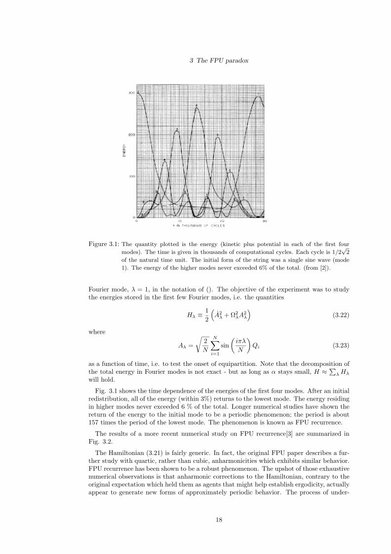
Figure 3.1: The quantity plotted is the energy (kinetic plus potential in each of the first four
modes). The time is given in thousands of computational cycles. Each cycle is 1/2√
2
of the natural time unit. The initial form of the string was a single sine wave (mode
1). The energy of the higher modes never exceeded 6% of the total. (from [2]).
Fourier mode, λ = 1, in the notation of (). The objective of the experiment was to studythe energies stored in the first few Fourier modes, i.e. the quantities
Hλ ≡ 12
(A2
λ + Ω2λA2
λ
)(3.22)
where
Aλ =
√2N
N∑
i=1
sin(
iπλ
N
)Qi (3.23)
as a function of time, i.e. to test the onset of equipartition. Note that the decomposition ofthe total energy in Fourier modes is not exact - but as long as α stays small, H ≈ ∑
λ Hλ
will hold.
Fig. 3.1 shows the time dependence of the energies of the first four modes. After an initialredistribution, all of the energy (within 3%) returns to the lowest mode. The energy residingin higher modes never exceeded 6 % of the total. Longer numerical studies have shown thereturn of the energy to the initial mode to be a periodic phenomenon; the period is about157 times the period of the lowest mode. The phenomenon is known as FPU recurrence.
The results of a more recent numerical study on FPU recurrence[3] are summarized inFig. 3.2.
The Hamiltonian (3.21) is fairly generic. In fact, the original FPU paper describes a fur-ther study with quartic, rather than cubic, anharmonicities which exhibits similar behavior.FPU recurrence has been shown to be a robust phenomenon. The upshot of those exhaustivenumerical observations is that anharmonic corrections to the Hamiltonian, contrary to theoriginal expectation which held them as agents that might help establish ergodicity, actuallyappear to generate new forms of approximately periodic behavior. The process of under-
18

3 The FPU paradox
Figure 3.2: FPU recurrence time, divided by N3 vs a scaling variable R = α(E/N)1/2N2 where
E/N ≈ [πB/(2N)]2 is the energy density. Typical values used by FPU correspond to
R À 1. The asymptotic regime is well described by the relationship Tr/N3 = R−1/2
(from Ref. [3]).
standing the source of this behavior - also known as the FPU paradox - and relating it toother manifestations of nonlinearity [4] has led to a profound change in theoretical physics.
19

4 The Korteweg - de Vries equation
4.1 Shallow water waves
Original context: Wave motion in shallow channels, cf. Scott-Russell1
Mathematical description due to Korteweg and deVries (KdV [6]). The equation arises inwide variety of physical contexts (e.g. plasma physics, anharmonic lattice theory). Hence itcounts as one of the “canonical” soliton equations.
Long waves (typical length l) in a shallow channel l À h.
Small amplitude (¿ h) waves (weak nonlinearity)
Two-dimensional fluid flow (motion in lateral dimension of channel neglected)
x: horizontal direction, y: vertical direction
4.1.1 Background: hydrodynamics
Fluid velocity~V ≡ ux + vy (4.1)
Equations of (Eulerian) incompressible fluid dynamics
• continuity equation∇ · ~V = 0 (4.2)
• Euler equation∂~V
∂t+ (~V · ∇)~V = −1
ρ∇p + ~g (4.3)
where ~g = −gy plus
• irrotational flow (no vortices)
∇× ~V = 0 ⇒ ~V = ∇Φ . (4.4)
Using vector identity
(~V · ∇)~V =12∇V 2 − ~V × (∇× ~V ) (4.5)
in (4.3) (only first term survives due to (4.4) ), and (4.4) in (4.2) transforms hydrodynamicsequations to1“I was observing the motion of a boat which was rapidly drawn along a narrow channel by a pair of horses,
when the boat suddenly stopped - not so the mass of water in the channel which it had put in motion; itaccumulated round the prow of the vessel in a state of violent agitation, then suddenly leaving it behind,rolled forward with great velocity, assuming the form of a large solitary elevation, a rounded, smoothand well-defined heap of water, which continued its course along the channel apparently without changeof form or diminution of speed. I followed it on horseback, and overtook it still rolling on at a rate ofsome eight or nine miles an hour, preserving its original figure some thirty feet long and a foot to a footand a half in height. Its height gradually diminished, and after a chase of one or two miles I lost it inthe windings of the channel. Such, in the month of August 1834, was my first chance interview with thatsingular and beautiful phenomenon which I have called the Wave of translation.”[5]
20

4 The Korteweg - de Vries equation
1. continuity4Φ = 0 , (4.6)
2. Euler∂Φ∂t
+12(∇Φ)2 +
p
ρ+ gy = 0 . (4.7)
4.1.2 Statement of the problem; boundary conditions
The above eqs (4.6) and (4.7) must now be solved subject to the boundary conditions
1. bottom: no vertical motion of the fluid
v(x, y = 0) = 0 ∀x (4.8)
2. top: free surface defined asy = h + η(x, t). (4.9)
Velocity of free boundary coincides with fluid velocity,
dy
dt=
∂η
∂t+
∂η
∂x
dx
dthence
v =∂η
∂t+
∂η
∂xu (4.10)
holds at the free surface.
The solution will involve two steps: first, find a general class of solutions of (4.6) whichsatisfy the bottom BC (4.8), and then use this general class to determine the height profile(4.9) by demanding that the Euler equation (4.7) be satisfied at the free surface, where p = 0holds. The Euler equation can then be used to determine the pressure at any point.
4.1.3 Satisfying the bottom boundary condition
Consider the general form of an expansion (the height O(h) is small in a sense which willbe made precise below) of the type
u = f(x) + f1(x)y + f2(x)y2 + f3(x)y3 + · · ·v = g1(x)y + g2(x)y2 + g3(x)y3 + · · · . (4.11)
The conditions ∂u∂y = ∂v
∂x and ∂u∂x = −∂v
∂y imposed by (4.6) can now be written, respectively,as
f1 + 2f2y + 3f3y2 = g1xy + g2xy2 (4.12)
andfx + f1y + f2y
2 = −g1 − 2g2y − 3g3y2 (4.13)
from which
f1 = 0 (4.14)2f2 = g1x (4.15)3f3 = g2x (4.16)
21

4 The Korteweg - de Vries equation
and
fx = −g1 (4.17)f1x = −2g2 (4.18)f2x = −3g3 (4.19)
follow. Using the second set in the first, results in f1 = 0, 2f2 = −fxx, 2f3 = −1/2f1xx(= 0);it follows that g2 = 0 and g3 = −1/3f2x = 1/3!fxxx. Collecting terms,
u = f − 12fxxy2 +O(y4) (4.20)
v = −fxy +13!
fxxxy3 . (4.21)
4.1.4 Euler equation at top boundary
Set p = 0 in (4.7) and differentiate with respect to x:
∂u
∂t+
12
∂
∂x(u2 + v2) + g
∂η
∂t= 0 . (4.22)
The problem is now to solve the system of coupled differential equations (4.22) and (4.10)using the expressions (4.20) and (4.21). Key: follow the scale of variation of the physicalquantities involved. First note that if the water height is not much different from h (smallnonlinearity), it will be useful to set
η = εhη (4.23)
Note ε is not a parameter of the problem. It simply serves as a “tag” to let us keeptrack of scales. At the end we will have to check the consistency of the assumptions andapproximations made.
According to our assumption, the length scale on which the fluid profile varies along the xdirection is of the order l À h. In order to incorporate this assumption in the approximation,I define a rescaled variable via
x = lx . (4.24)
Dimensional consideration determine a natural velocity scale c =√
gh. The motion shouldbe slow with respect to that scale - in agreement with small amplitude variations of theprofile. In other words, we expect u ¿ c. Note that from the leading orders of (4.20) and(4.21)it follows that v is typically of order h/l ≡ δ smaller than u. It is therefore reasonableto rescale
f = εcf (4.25)u = εcu (4.26)v = δεcv . (4.27)
Finally I use a rescaled timet = t l/c . (4.28)
With these rescalings, keeping lowest order terms, i.e. of O(ε) and O(δ2), the rescaledequations (4.20) and (4.21) become - on the surface -
u = f − 12δ2fxx (4.29)
v = −(1 + εη)fx +16δ2fxxx ; (4.30)
22

4 The Korteweg - de Vries equation
accordingly, the top boundary condition (4.10) and the Euler equation (4.22) transform to
fx + ηt + ε(f η)x − 16δ2fxxx = 0 (4.31)
ft + ηx +ε
2(f2)x − 1
2δ2fxxt = 0 . (4.32)
First we note that in the absence of nonlinearity (ε = 0) and dispersion (δ = 0), freewave propagation with unit velocity (in dimensionless units) occurs; in that (zeroth) order,f = η. But of course this is hypothetical because δ and ε are not parameters of the problem- they just help us keep track of things! However, the zeroth order approximation is usefulin the sense that it suggests a coordinate transformation which absorbs the fastest timedependence; let
ξ = x− t (4.33)τ = εt . (4.34)
Keeping terms to first order in ε and δ2, we use the property
ηx = ηξ (4.35)ηt = −ηξ + ητ ε (4.36)
(which holds for f as well) transform the system (4.32) to
fξ − ηξ + εητ + ε(η2)ξ − 16δ2ηξξξ = 0 (4.37)
−fξ + ηξ + εητ +ε
2(η2)ξ +
12δ2ηξξξ = 0 . (4.38)
where we have used the property f = η in terms which contain ε or δ2 factors. The sum of(4.38) is
2εητ +32ε(η2)ξ +
13δ2ηξξξ = 0 . (4.39)
The three terms in (4.39) will be of the same order if δ2 = O(ε), i.e. if the nonlinearitybalances the dispersion. We choose ε = δ2/6. Note that the choice must be tested at theend to check whether it satisfies the original requirements (small amplitude, long waves).With this choice and the substitution η = 4φ I arrive at the “canonical” KdV form,
φτ + 6φφξ + φξξξ = 0 . (4.40)
4.1.5 A solitary wave
At this stage, without recourse to advanced mathematical techniques, it is possible to followthe path of KdV and look for special, exact, propagating solutions of (4.40) of the type φ(s),where s = ξ − λτ . (4.40) becomes
−λφs + 3(φ2)s + φsss = 0 (4.41)
which has an obvious first integral
−λφ + 3φ2 + φss = const. (4.42)
If we are looking for solutions which vanish at infinity (lims→∞ φ(s) = 0 and lims→∞ φs(s) =0) the constant will be zero, i.e.
φss = λφ− 3φ2 =d
dφ(12λφ2 − φ3) (4.43)
23

4 The Korteweg - de Vries equation
Multiplying both sides by 2φs we can integrate once more, obtaining
φ2s = λφ2 − 2φ3 (4.44)
where the integration constant must vanish once again (cf. above). Note that, if a solutionexists, the parameter λ must be > 0 and φ < λ/2. Taking the square root of (4.44) andinverting the fractions I obtain
ds = ± dφ
φ√
λ− 2φ(4.45)
which can be integrated directly, resulting in
φ(s) =λ
2 cosh2[√
λ2 (s− s0)
] (4.46)
where s0 is an arbitrary constant. (The plus sign in (4.45) has been chosen for s < s0 andthe minus for s > s0).
Note that the properties of the propagating solution (4.46) - except for its initial position,which is determined by s0 - are all governed by a single parameter. If the velocity λ isgiven, the amplitude is fixed at λ/2 and the spatial extent at 2λ−1/2. In other words - in thecanonical units of (4.40) - a slow pulse will also have a small amplitude and a large spatialextent.
4.1.6 Is the solitary wave a physical solution?
Eq. (4.46 ) is an exact, propagating, pulse-like solution of (4.40). But is it an acceptablesolution of the original problem? In other words, is the surface profile of low amplitude and isit a long wave? To do this, we have to go back to the original variables, and convince ourselvesthat (4.46) generates (some) acceptable solutions for the original problem (Exercise)
4.2 KdV as a limiting case of anharmonic lattice dynamics
Consider the 1-d anharmonic chain; atomic displacements are denoted by un; neighboringatoms of mass m interact via anharmonic potentials of the type
V (r) =12kr2 +
13kbr3 (4.47)
where r is the distance between nearest neighbors. The equations of motion are
mqn = − ∂
∂qn[V (qn+1 − qn) + V (qn − qn−1]) (4.48)
= k(qn+1 + qn−1 − 2qn)− kb[−(qn+1 − qn)2 + (qn − qn−1)2]= k(qn+1 + qn−1 − 2qn)− kb(qn+1 + qn−1 − 2qn)(qn+1 − qn−1) .
If the displacements do not vary appreciably on the scale of the lattice constant a, we canuse a continuum approximation; keeping terms of fourth order in the lattice constant,
mq ≡ qtt = ka2qxx + ka4 24!
qxxxx + kba2qxx 2aqx ,
where x = na is the continuum space variable; defining c2 = ka2/m, this can be written as
1c2
qtt − qxx =112
a2qxxxx + 2αqxqxx , (4.49)
24

4 The Korteweg - de Vries equation
where α = ab provides a dimensionless measure of the anharmonicity.
I now look for solutions which vary smoothly in space, i.e. over a typical length of manylattice spacings, and where the main time dependence is contained in the wave equationpart, i.e. of the form
q(ξ, τ) ≡ q(εx− ct
a, δω0t) , (4.50)
where ω0 = c/a =√
k/m, ε ¿ 1 and δ ¿ ε; the exact dependence of δ on ε will be fixedlater.
The relevant derivatives transform according to
qx =ε
aqξ
qxx =( ε
a
)2
qξξ
qxxx =( ε
a
)3
qξξξ
qtt = ω20
(ε2qξξ − 2εδqξτ +O(δ2)
).
Using them in (4.49) gives
2δqξτ +112
ε3qξξξξ + 2αqξqξξ = 0 , (4.51)
which, after a rescalingqξ(=
a
εqx) = − ε
4αaφ (4.52)
and setting 2
δ =124
ε3
can be reduced to the canonical KdV form
φτ − 6φφξ + φξξξ = 0 . (4.53)
Note that the rescaling of length, i.e. the value of the small parameter ε is still a matter offree choice, depending on the (initial) conditions of the problem.
The above analysis shows that one may legitimately suspect that nonlinear propagatingsolitary waves will be generic in anharmonic lattices, at least for certain parameter ranges.Again, one has to make sure that the solutions found from solving the KdV equation (4.53)are appropriate for the original problem (4.49) (check consistency of approximations made).
4.3 KdV as a field theory
4.3.1 KdV Lagrangian
The KdV equationut − 3(u2
x)x + uxxx = 0 (4.54)
can be derived from the Lagrangian
L =∫
dxL(φ, φt, φx, φxx) (4.55)
2note that this guarantees δ ¿ ε as demanded above.
25
4 The Korteweg - de Vries equation
where
L =12φxφt − φ3
x −12φ2
xx . (4.56)
Note that because the Lagrangian density depends on the second derivative of the field,(1.42) contain an extra term
− d2
dx2
(∂L
∂φxx
). (4.57)
Minimization of the action leads to the field equations of motion
φxt − 3(φ2x)x + φxxxx = 0 (4.58)
which reduces to (4.54) upon the substitution
φx = u . (4.59)
Continuous symmetries of the Lagrangian will again give rise to an equation like (1.44), withan extra term
∂L∂φxx
δφxx (4.60)
on the left-hand side. The above modifications generate an extra contribution
∂L∂φxx
δφxx − d2
dx2
(∂L
∂φxx
)δφ (4.61)
to the left-hand side of (1.45).
4.3.2 Symmetries and conserved quantities
For some infinitesimal transformations (cf. section ) one can verify explicitly that δφxx =d2δφ/dx2. If this is the case, the integral over all space of the extra contribution (4.61) caneasily be seen to vanish (repeated integration by parts of either of the two terms). In thiscase, the standard symmetries are reflected in the same standard conservation (with thesame densities of conserved quantities), as in section .... .
Translational invariance in space
Conservation of the total momentum
P = −∫ ∞
−∞dx
∂L∂φt
φx = −12
∫ ∞
−∞dx φ2
x = −12
∫ ∞
−∞dx u2 . (4.62)
Translational invariance in time
Conservation of the total energy
H =∫ ∞
−∞dx
(∂L∂φt
φt − L)
= −∫ ∞
−∞dx
(12φ2
xx + φ3x
)
= −∫ ∞
−∞dx
(12u2
x + u3
). (4.63)
26
4 The Korteweg - de Vries equation
Conservation of mass
The symmetry φ → φ + ε generates δφ = ε, and all other variations are zero. From (1.45),conservation of
M =∫ ∞
−∞dx
∂L∂φt
=12
∫ ∞
−∞dx φx =
12
∫ ∞
−∞dx u , (4.64)
the total “mass”, is deduced.
Galilei invariance
The transformation x → x− εt, φ(x, t) → φ(x− εt)− εx (or in terms of the u-field, u(x, t) →u− ε, generates (cf. section ....)
x → x− εt
δφ = φ(x− εt)− φ(x)− εx = −εtφx − εx
δφt = φt(x− εt)− φt(x) = −εtφxt
δφx = φx(x− εt)− φx(x)− ε = −εtφxx − ε
δL =dLdx
δx = −dLdx
εt ⇒ J1 = −tL , J0 = 0 . (4.65)
Owing to δφxx = (δφ)xx there are no extra terms in the conserved currents. Eq. (1.45)applies. Since δφx = (δφ)x the two last terms in the left-hand side of (1.45) combine toform a total space derivative; similarly, because of δφt = (δφ)t, the first two terms combineto form a total time derivative, i.e. the conserved density is
∂L∂φt
δφ/ε =12φx(−tφx − x) , (4.66)
or, integrating over all space, and dividing by the total mass M ,
X =1M
∫ ∞
−∞dx x
u
2=
P
Mt + const. (4.67)
which expresses the fact that the center of mass moves at a constant velocity.
4.3.3 KdV as a Hamiltonian field theory
27
5 Solving KdV by inverse scattering
5.1 Isospectral property
Given the KdV equationut − 6uux + uxxx = 0 (5.1)
and a well behaved initial condition u(x, 0), which vanishes at infinity, it is possible todetermine the time evolution u(x, t) in terms of a general scheme, which is known as inversescattering theory.
The scheme is based on the following particular property of (5.1):
Given the linear operatorL(t) = −∂2
xx + u(x, t) (5.2)
whose parametric time dependence is governed by (5.1), and the associated eigenvalue equa-tion
L(t)ψj(x, t) = λj(t)ψj(x, t) , (5.3)
it can be shown thatdλj
dt= 0 . (5.4)
5.2 Lax pairs
The “isospectral” property can be formulated somewhat more generally: Suppose we canconstruct a linear, self-adjoint operator B = B†, dependent on u and such that
iLt ≡ idL
dt≡ i lim
∆→0
L(t + ∆)− L(t)∆
= [L,B] (5.5)
holds as an operator identity, i.e.
iLtf = [L,B]f ∀f ⇔ (5.1) . (5.6)
The operators L and B are then called a Lax pair. The time evolution of L is governed by
L(t) = U(t)L(0)U† (5.7)
whereU = eiBt . (5.8)
Consider (5.3) at t = 0, and apply the operator U(t) to both sides from the left, i.e.
U(t)L(0) U†(t)U(t)ψj(0) = λj(0)U(t)ψj(0) (5.9)
where, in addition I have inserted a factor U†U = 1. It can be recognized immediately thatthe l.h.s. of (5.9) and (5.3) are identical, provided
ψj(t) = U(t)ψj(0) , (5.10)
28

5 Solving KdV by inverse scattering
and that, in order for the r.h.sides to coincide, I must have
λ(t) = λ(0) ∀t (5.11)
(isospectral property).
The form of the operator B in the KdV case is
B = 4i∂3xxx − 3i (u∂x + ∂xu) (5.12)
(verify explicitly (5.6).
5.3 Inverse scattering transform: the idea
The isospectral property tentatively suggests that it might possible to proceed as follows:
• solve the linear problem (5.3) at time t = 0, i.e. determine the eigenvalues λj andthe eigenfunctions ψj(x, 0) from the known u(x, 0).
• determine the evolution of the eigenfunctions from (5.10) at a later time t.
• try to solve the “inverse problem” of determining the “potential” u(x, t) from theknown spectra and eigenfunctions at the time t.
In fact, the last step is the well known problem of inverse scattering theory in quantummechanics, where physicists had tried to extract information on the nature of interparticleinteractions from analyzing particle scattering data. The one-dimensional problem (corre-sponding to a spherically symmetric potentials in 3 dimensions) was completely solved inthe 1950’s (Gel’fand, Levitan & Marchenko). I will present the solution below, but beforedoing that, let me outline some broad features:
“Scattering data”in the mathematical sense are the asymptotic properties of the solutionof the associated linear problem, i.e. the properties far from the source of scattering, wherethe potential is effectively zero. What GLM have shown is that you can reconstruct thepotential from the scattering data. Furthermore, it turns out that the operator B takesan especially simple form in the asymptotic limit, which allows us to write down an exact,analytic formula for the time evolution of scattering data. Evolution of the scattering datais the easy part of the game. But then if I only need scattering data at time t, and I knowhow these data evolve in time, all the input I need is the scattering data for the potentialu(x, 0). This is exactly the program of the inverse scattering transform (IST). Because it isbased only on the asymptotic part of the solution of the associated linear problem, it canbe written down in closed form. I summarize the IST program schematically:
1. determine the scattering data S of the linear problem (5.3) at time t = 0, from theknown u(x, 0).
2. determine the evolution of the scattering data S(t) at a later time t from the asymptoticfrom of the operator B.
3. do the inverse problem at time t, i.e. determine the potential u(x, t) from the knownscattering data S(t).
5.4 The inverse scattering transform
5.4.1 The direct problem
This is just a summary of properties known from elementary quantum mechanics.
29

5 Solving KdV by inverse scattering
Jost solutions
The linear eigenvalue problem[− ∂
∂x2+ u(x)
]ψ(x) = k2ψ(x) (5.13)
has, in general, a discrete and a continuum spectrum, corresponding to imaginary and realvalues of k respectively. For real k there are in general two linearly independent solutions.Such a linearly independent set is provided by the Jost solutions:
f1(x, k) ∼ eikx x →∞f2(x, k) ∼ e−ikx x → −∞ . (5.14)
The Jost solutions of (5.13) satisfy the integral equations
f1(x, k) = eikx −∫ ∞
x
dx′G(x, x′)f1(x′, k)
f2(x, k) = e−ikx +∫ x
−∞dx′G(x, x′)f2(x′, k) (5.15)
where
G(x, x′) =sin k(x− x′)
ku(x′) . (5.16)
Eqs. (5.15) can be analytically continued to the upper half plane of complex k. Someinformation on the analytic properties can be obtained by considering the lowest iteration,where we substitute f1(x′, k) = eikx′ in the r.h.s. of the first equation. This gives
f1(x, k) ≈ eikx −∫ ∞
x
dx′eik(x′−x) − e−ik(x′−x)
2iku(x′)eikx′
≈ eikx − eikx 12ik
∫ ∞
x
dx′ 1− e2ik(x′−x)u(x′) (5.17)
which can be thought of as the beginning of a systematic expansion in inverse powers of k.Note that since x′ − x > 0, the exponential will be convergent in the upper-half plane of k;therefore, if the potential vanishes sufficiently rapidly at infinity, I estimate
g1(x, k) ≡ f1(x, k)− eikx ∼ eikxh(x, k) (5.18)
where h vanishes as 1/k for high values of k.
The propertyf2(x, k) = a(k)f1(−k, x) + b(k)f1(k, x) . (5.19)
will be useful.
For bound states, corresponding to k = iκ, the Jost solutions are degenerate.
Asymptotic scattering data
The asymptotic (scattering) data of (5.3) is defined as follows:
• discrete spectrum (bound states)
λn = −κ2n n = 1, · · · , N , (5.20)
30

5 Solving KdV by inverse scattering
where κn > 0;
ψn(x) = f1(x, k) ∼ e−κnx x →∞= Cnf2(x, k) ∼ Cneκnx x → −∞ . (5.21)
I will also need the normalization integral of each bound state
1αn
=∫ ∞
−∞dxψ2
n(x) =∫ ∞
−∞dxf2
1 (x, iκn) (5.22)
• continuous spectrum (scattering states)
λ(k) = k2 −∞ < k < ∞ . (5.23)
The “physical ”scattering states corresponding to waves incident from the right, are
ψ(x, k) ∼ e−ikx + R(k)eikx x →∞∼ T (k)e−ikx x → −∞ . (5.24)
where R(k), T (k) are, respectively, the reflection and transmission coefficients, whichsatisfy
|R(k)|2 + |T (k)|2 = 1 .
The Jost solutions are related to the physical solution (5.24) via
ψ(x, k) = T (k)f2(x, k) = f1(x,−k) + R(k)f1(x, k) ∀x. (5.25)
This identifies a(k) = 1/T (k) and b(k) = R(k)/T (k).
The complete set of scattering data for any one dimensional potential of a Schroedinger-typeequation is
S ≡ [κn, Cn, αn, n = 1 · · · , N ; T (k), R(k)]. (5.26)
In fact, for the purposes of performing the inverse scattering transform I will only need thereduced set 1
S ≡ [κn, αn, n = 1 · · · , N ; R(k)] (5.27)
5.4.2 Time evolution of scattering data
I promised this will be the easy part. The operator B has the property
lim|x|→±∞
= B∗ = 4i∂3xxx . (5.28)
Since∂
∂tψj(x, t) = iBψj(x, t) (5.29)
holds for all eigenfunctions, we can apply in the asymptotic regime, where B ∼ B∗.
• In the case of a discrete eigenfunction, this gives
ψn(x) ∼ e−κnx+4κ3nt x →∞
∼ Cneκnx−4κ3nt x → −∞ , (5.30)
1Note that if scattering theory is to make sense, the potential must be vanishing at (±)infinity. I have notspecified the minimal exact mathematical conditions which satisfy this demand.
31

5 Solving KdV by inverse scattering
or, in keeping with the agreed normalization of the type (5.21), I multiply with a factore−4κ3
nt, and obtain
ψn(x) ∼ e−κnx x →∞∼ Cn(t)eκnx x → −∞ , (5.31)
withCn(t) = Cn(0)e−8κ3
nt . (5.32)
• In the case of Jost solutions I obtain
f1(k, x) ∼ eikx+4ik3t x →∞f2(k, x) ∼ e−ikx−4ik3t x → −∞ ; (5.33)
the physical solution therefore evolves according to
ψ(k, x) ∼ e−ikx−4ik3t + R(k)eikx+4ik3t x →∞∼ T (k)e−ikx−4ik3t x → −∞ ,
or, multiplying both by a factor e4ik3t, to keep the standard normalization of ()
ψ(k, x) ∼ e−ikx + R(k, t)eikx x →∞∼ T (k)e−ikx x → −∞ ,
whereR(k, t) = R(k)e8ik3t . (5.34)
The scattering data evolve according to (5.32) and (5.34). The transmission coefficient T (k)stays constant in time.
5.4.3 Reconstructing the potential from scattering data (inversescattering problem)
Reconstruction of the potential from scattering data is an old problem in quantum me-chanics. A complete solution has been given in one dimension, subject to fairly generalconditions, by Gelfand and Levitan [7] and Marchenko[8]. Reviews by Faddeyev[9] andScott[10]. Definition of the problem: Given the eigenvalue equation
[− d2
dx2+ u(x)
]ψ(x) = k2ψ(x) (5.35)
determine u(x) from scattering data in the form of eqs. (5.27).
Fourier transforms of the g(x, k) functions
gj(x, y) =12π
∫ ∞
−∞dk e−ikygj(x, k) , (5.36)
where j = 1, 2, with an inverse
gj(x, k) =∫ ∞
−∞dy eiky gj(x, y) . (5.37)
Note that, due to the analytic properties of f1 (cf. (5.18), which allows to close the contourof (5.36) from above without finding any singularities)
g1(x, y) = 0 if y < x . (5.38)
Similarly,g2(x, y) = 0 if y > x . (5.39)
32

5 Solving KdV by inverse scattering
Relating g1(x, x) to the potential u(x)
The starting point is to recognize that(
∂2
∂x2+ k2 − u
)g1(x, k) =
(∂2
∂x2+ k2 − u
)(f1(x, k)− 1) = u(x)eikx ; (5.40)
multiplying both sides by e−iky/2π and integrating over all k, I obtain(
∂2
∂x2− ∂2
∂y2− u(x)
)g1(x, y) = u(x) δ(x− y) ; (5.41)
defining new variables ζ = (x + y)/2, η = y − x, I use ∂2x − ∂2
y = 2∂η∂ζ , to transform (5.41)to
−2∂2
∂η∂ζg1
(ζ − η
2, ζ +
η
2
)− u
(ζ − η
2
)g1
(ζ − η
2, ζ +
η
2
)
= u(ζ − η
2)δ(−η) ,
which can be integrated over an interval of length ε around η = 0. The result is
−2∂
∂ζg1(ζ, ζ)− εu(ζ)g1(ζ, ζ) = −u(ζ) , (5.42)
which in the limit ε → 0 becomes
u(x) = −2d
dxg1(x, x) (5.43)
where I have reverted to the original variables.
Relating g1(x, y) to the scattering data
Define Fourier transforms
T (y) =∫ ∞
−∞
dk
2πe−iky[T (k)− 1] (5.44)
R(y) =∫ ∞
−∞
dk
2πeikyR(k) . (5.45)
Rewrite (5.25) as
T (k)f2(x, k) = f1(x,−k) + R(k)[f1(x, k)− eikx + eikx
]; (5.46)
adding −f2(x, k) to both sides and adding and subtracting e−ikx to the right hand side gives
(T (k)− 1) f2(x, k) = g1(x,−k)− g2(x, k) + R(k)g1(x, k) + R(k)eikx ; (5.47)
multiplying both sides by eiky/2π and integrating over all k produces∫ ∞
−∞
dk
2πeiky [T (k)− 1] f2(x, k) = g1(x, y)− g2(x, y) +
∫ ∞
−∞dy′ R(y + y′) g1(x, y′) + R(x + y) (5.48)
Lemma: T (k) has only simple poles
33

5 Solving KdV by inverse scattering
It can be shown that the transmission coefficient T (k) is analytic in the upper half plane,including the real axis, except for simple poles which correspond to the bound states, i.e. atk = iκn. In the neighborhood of such a pole
T (k) ≈ iCnαn
k − iκn, (5.49)
where1
αn=
∫ ∞
−∞dx[f1(x, iκn)]2 (5.50)
is the normalization integral of the bound state.
Using the above lemma, it is possible to compute the integral in the left-hand side of(5.48) by closing the contour from above. The contribution from each bound state is
2πie−κnyi12π
Cnαn f2(x, iκn) = −αn e−κnyf1(x, iκn)
= −αn e−κnyg1(x, iκn)− αn e−κn(x+y)
where I have used the fact that Jost states are degenerate if k = κn (cf. Eq. (5.21)).Moreover, I only need (5.48) for x ≤ y, since otherwise g1(x, y) = 0. Defining a combinedkernel which incorporates all scattering data,
K(z) = R(z) +N∑
n=1
αn e−κnz , (5.51)
I finally obtain
g1(x, y) + K(x + y) +∫ ∞
−∞dy′ K(y + y′) g1(x, y′) = 0 if x ≤ y (5.52)
g1(x, y) = 0 if x > y (5.53)
(Gel’fand, Levitan, Marchenko equation).
5.4.4 IST summary
In order to solve the initial value problem of the KdV equation (5.1) we proceed as follows:
• Extract initial scattering data for the associated linear problem (5.13),
κn, αn;n = 1 · · · , N, R(k),−∞ < k < ∞ (5.54)
from potential u(x) at time 0.
• Define the scattering kernel at time t:
K(z; t) =∫ ∞
−∞
dk
2πeikz+8ik3tR(k) +
N∑n=1
αn e−κnz+8κ3nt . (5.55)
• Solve the Gel’fand, Levitan, Marchenko equation for x ≤ y,
g1(x, y; t) + K(x + y; t) +∫ ∞
x
dy′ K(y + y′; t) g1(x, y′; t) = 0 . (5.56)
• Extract the limitu(x, t) = −2
d
dxg1(x, x+; t) . (5.57)
Note that (i) I have explicitly included the parametric dependence on time, and (ii)the normalization integral αn has a time dependence such that the product Cnαn staysconstant (cf. time-independence of the transmission coefficient).
34
5 Solving KdV by inverse scattering
5.5 Application of the IST: reflectionless potentials
Suppose the scattering kernel (5.51) contains only bound states, i.e. R(k) = 0. This wouldcorrespond to a reflectionless potential in the original quantum mechanical context. In thiscase it turns out that I can systematically derive a whole class of solutions to the originalKdV equation by just solving the GLM equation (5.56) and taking the appropriate limit(5.57).
5.5.1 A single bound state
The scattering kernel has the form
K(z; t) = αe−κz+8κ3t . (5.58)
I will look for solutions of (5.56) which are separable, i.e.
g1(x, y; t) = e−κy h(x, t) ; (5.59)
with the above Ansatz, (5.56) tranforms to
h(x, t) + αe8κ3t
[e−κx + h(x, t)
∫ ∞
x
dy′e−2ky′]
= 0 ;
inserting the expression for the integral, (2κ)−1e−2κx, and setting α = 2κe2δ, I obtain
h(x, t)[1 + e2δe−2κx+8κ3t
]= −αe−κx+8κ3t
g1(x, y; t) = −2κe−κ(x+y)+8κ3t+2δ
1 + e−[2κx−8κ3t−2δ];
the limiting form for y = x is
g1(x, x; t) = −2κ1
1 + e2[κx−4κ3t−δ];
it follows that
u(x; t) = −2d
dxg1(x, x; t) = − 2κ2
cosh2[κ(x− 4κ2t)− δ](5.60)
which is identical to the solitary wave (4.46), if we identify λ in (4.46) with 4κ2 in (5.60).
Comments:
• the velocity of the wave corresponds (to within a factor of -4) to the eigenvalue of theassociated problem.
• The velocity coincides with the ratio P/M (cf. symmetries conservation laws; showthis (exercise)).
• Note that I made no attempt to guess the form of the wave. The form was “imposed” bythe separation ansatz (5.59), i.e. it is “built-in” in the association of the KdV equationwith the linear eigenvalue problem. This will be useful in the next subsection, whereI will try to construct solutions that correspond to multiple bound states.
• It is of course possible to treat the “proper” initial value problem. Starting with anylocalized potential which may support a bound state, one can perform the IST steps.Exercise: do this (i) for an attractive delta function potential −µδ(x), and (ii) for apotential of the type −N(N + 1)sech2x, where N is an integer; (hint: in case (ii) theform of the solution is an example of the case discussed in the next subsection).
35
5 Solving KdV by inverse scattering
5.5.2 Multiple bound states
Again, I will restrict myself to the case where the reflection coefficient vanishes. The scat-tering kernel has the form
K(z; t) =N∑
i=1
αi(t) e−κiz . (5.61)
where αi(t) = αie8κ3
i t carries the time dependence. A generalized form of the separationansatz (5.59)
g1(x, y; t) =N∑
i=1
e−κiy hi(x, t) (5.62)
transforms the GLM equation (5.56) to
N∑
i=1
e−κiy hi(x, t) + αi(t)e−κix +N∑
j=1
αi(t)κi + κj
e−(κi+κj)xhj(x, t) = 0 ,
which must hold for all y > x; hence, in nonsymmetric matrix form,
N∑
j=1
Aijhj(x, t) = Ci(x, t) (5.63)
where
Aij(x, t) = δij +αi(t)
κi + κje−(κi+κj)x (5.64)
andCj(x, t) = −αi(t)e−κix . (5.65)
Thus
hj =1
det Adet
A11 A12 · · · C1 A1 j+1 · · ·A21 A22 · · · C2 A2 j+1 · · ·· · · · · C3 · · · ·
···
. (5.66)
where the jth column in the matrix A has been substituted by the vector C; it follows that
g1(x, x) =1
detA
N∑
j=1
det
A11 A12 · · · C1e−κjx A1 j+1 · · ·
A21 A22 · · · C2e−κjx A2 j+1 · · ·
· · · · · C3e−κjx · · · ····
; (5.67)
note however that, since
dAij
dx= −αie
−(κi+κj)x = Cie−κjx ,
this is equivalent to
g1(x, x) =d
dxln det A . (5.68)
36

5 Solving KdV by inverse scattering
At this stage it is convenient to introduce the symmetrized form of the matrix A, obtainedby A = DAD−1, where Dij = (αi)−1/2δij , i.e.
Aij(x, t) = δij +(αiαj)1/2
κi + κje−(κi+κj)x , (5.69)
whereupon
u(x, t) = −2d2
dx2ln det A (5.70)
where I have reintroduced the time dependence, with the understanding that it arises solelyfrom the αi s.
Application: N = 2, the two-soliton solution
In the case N = 2
det A = 1 +α1
2κ1e−2κ1x +
α1
2κ1e−2κ2x +
α1α2
4κ1κ2
(κ1 − κ2
κ1 + κ2
)2
e−2(κ1+κ2)x
or, settingκ1 − κ2
κ1 + κ2≡ e−∆ , αj ≡ 2κj e2θj+∆ , (5.71)
det A = 1 + e−2(κ1x−θ1−∆2 ) + e−2(κ2x−θ2−∆
2 ) + e−2[(κ1+κ2)x−(θ1+θ2)] . (5.72)
Note that now the time dependence is carried by the θj ’s, i.e.,
θj → θj(t) = θ0j + 4κ3
j t (5.73)
In order to extract the asymptotic behavior of u(x, t) at early and late times, I proceed asfollows: Assume κ1 > κ2 without loss of generality. Then as, t → −∞, at sufficiently earlytimes, it is possible to satisfy the double inequality
θ1
κ1¿ θ2
κ2.
It is easy to see that, unless x ≈ θ1κ1
or x ≈ θ2κ2
, the 2nd derivative of the expression (5.72)will be vanishingly small. This is true
• for x À θ2κ2
, because the last three terms vanish, leaving det A = 1
• for x ¿ θ1κ1
, because, although the three last terms are all exponentially large, the lastone will be dominant. This leaves ln det A ∝ x and the second derivative vanishes.
• for θ1κ1¿ x ¿ θ2
κ2the second term will be exponentially small, and the third term be
much larger than the last. Again, ln det A ∝ x and the second derivative vanishes.
This leaves the cases where x is appreciably near either θ1κ1
or θ2κ2
. In the first case, thecontributions to (5.72) come from the 3rd and 4th terms, i.e.
det A ≈ e−2(κ2x−θ2−∆2 )
[1 + e−2(κ1x−θ1+
∆2 )
],
or,
ln det A ≈ −2(κ2x− θ2 − ∆2
)− (κ1x− θ1 +∆2
) + ln[2 cosh(κ1x− θ1 +
∆2
)]
,
37

5 Solving KdV by inverse scattering
-5
0
5
0.0
0.5
t
κ1=2
κ2=1
θ1
0/κ1= -2.
θ2
0/κ2= -1.
x
-5 0 5
-0.2
0.0
0.2
0.4
0
1.000
1.950
3.000
4.000
5.000
6.000
7.000
8.000
x
t
Figure 5.1: The two-soliton solution [−u(x, t)] of the KdV equation as a function of space and time.
Left panel: a 3-d plot shows the collision of the two solitons. Right panel: a contour
plot of the same function; note the asymptotic motion of the local maxima and the
phase shifts as a result of the interaction.
and henceu(x, t) ≈ −2κ2
1 sech2(κ1x− θ1 +∆2
) if x ≈ θ1/κ1
Similarly, it can be shown that
u(x, t) ≈ −2κ22 sech2(κ2x− θ2 − ∆
2) if x ≈ θ2/κ2 .
Combining the above, and reintroducing the explicit time dependence, I can write that
u(x, t) ∼ −22∑
j=1
κ2j sech2(κjx− 4κ3
j t− θ0j ±
∆2
) if t → −∞ , (5.74)
where the upper sign holds for j = 1, and the lower for j = 2. The above analysis can berepeated almost verbatim for asymptotically late times and leads to
u(x, t) ∼ −22∑
j=1
κ2j sech2(κjx− 4κ3
j t− θ0j ∓
∆2
) if t →∞ . (5.75)
The above equations describe the soliton property in a mathematically exact fashion. As wefollow the evolution from very early to very late times, we see the larger - and faster - localcompression reach the smaller - and slower - , interact with it in an apparently intricatefashion, and then disengage itself and resume its motion with the same velocity. Both wavesmaintain shape, amplitude and speed. The interaction does however leave a signature. Thecenter of mass of each wave becomes slightly displaced; the fastest by an amount of ∆/κ1
38
5 Solving KdV by inverse scattering
(forwards), the slower by an amount of −∆/κ2 (backwards). Note that because the massof each soliton is proportional to κj , the center of mass of the combined two-soliton systemmoves at a constant speed before and after the two-soliton collision. This type of elastic,transparent interaction which leaves velocities unchanged and results only in spatial shifts2
is characteristic of soliton bearing systems, and accounts for their remarkable dynamicalproperties.
The analysis can be generalized to the N−soliton solution. It can be shown that phaseshifts are pairwise additive, i.e. the total phase shift of any soliton as a result of its interactionwith the other N − 1 solitons is the sum of the N − 1 phase shifts resulting from the N − 1collisions.
Fig. 5.1 exhibits graphically the dependence of the two-soliton solution on space and time.
5.6 Integrals of motion
It is possible to deal with integrals of motion in a systematic fashion, by following theanalytic structure of the scattering data. Recall that the transmission coefficient does notcarry any time dependence under the IST, i.e. it can be treated as a constant of the motion!
5.6.1 Lemma: a useful representation of a(k)
Given the fact that a(k) (recall that a is the inverse of the transmission coefficient) hassimple zeros in the upper half of the complex plane, the following identity holds:
ln a(k) =1
2πi
∫ ∞
−∞dk′
ln |a(k′)|2k′ − k
+N∑
j=1
ln
(k − kj
k − k∗j
)(5.76)
(cf. appendix ...).
5.6.2 Asymptotic expansions of a(k)
The asymptotic expansion
ln a(k) ∼∞∑
n=1
Jn
(2ik)n(5.77)
holds for |k| > max|kj |.Multiply both sides of (5.77) by kl−1/(2πi) and integrate over a circle of radius R >
max|kj | centered at the origin of the complex k-plane. The only term which survives inthe sum is that with j = l, hence
(2i)−lJl =1
2πi
∮dk kl−1 ln a(k) ;
performing the dk integration in the first term of (5.76) generates a contribution −k′ l−1.The second term can be integrated by parts and generates contributions from all poles. Thisresults in
Jl
(2i)l= − 1
2πi
∫ ∞
−∞dk kl−1 ln |a(k)|2 +
N∑
j=1
1l
(k∗ l
j − klj
). (5.78)
2the term “phase shifts” is generically applicable.
39

5 Solving KdV by inverse scattering
So far this has been general. Applying to the KdV equation, I set kj = iκj ; note that theterms in the discrete sum vanish if l is even. Due to the reflection symmetry |a(k)| = |a(−k)|,the integrals vanish as well for even l. This leaves
J2m+1
22m+1= −(−1)m
∫ ∞
−∞dk k2m ln |a(k)|2 + 2
N∑
j=1
κ2m+1j
2m + 1. (5.79)
In what follows, I will relate the Jls - which are by definition constants of the motion, sincethey only depend on a(k) and bound state eigenvalues - to the family of conserved quantitiesgenerated in the previous section, independently of the IST.
From the general property of the Jost functions
f2(x, k) = a(k)f1(x,−k) + b(k)f1(x, k) (5.80)
I deduce that if Imk > 0lim
x→∞[f2(x, k)eikx
]= a(k) . (5.81)
This is because in the limit of large positive x the first term in (5.80), f1(x,−k) ∼ e−ikx isexponentially large and the second f1(x,−k) ∼ e−ikx is exponentially small. On the otherhand,
limx→−∞
[f2(x, k)eikx
]= 1 . (5.82)
holds by definition. Knowledge of the two limits allows me to define
σ(x) =d
dx
[ln
f2(x, k)eikx
]=
f ′2f2
+ ik (5.83)
with the property ∫ ∞
−∞dx σ(x) = ln a(k) . (5.84)
Now we can use the fact that f2 is a solution of the associated linear problem, to derivea differential equation for σ in terms of u. To do this I multiply both sides of (5.83) anddifferentiate with respect to x. This gives
f ′′2 + ikf ′2 = f ′2σ + f2σ′ ,
oruf2 − k2f2 + ikf ′2 = f ′2σ + f2σ
′ ;
substituting f ′2 = (σ − ik)f2 generates
σ′ − 2ikσ + σ2 − u = 0 (5.85)
a nonlinear ordinary first order differential equation of the Ricatti type.
I can now try to generate an asymptotic solution of the Ricatti equation (5.85),
σ(x, k) ∼∞∑
n=1
σn(x, k)(2ik)n
(5.86)
where I note that, because of (5.77) and (5.84),∫ ∞
−∞dx σn(x) = Jn . (5.87)
40

5 Solving KdV by inverse scattering
Indeed, I note that the asymptotic ansatz (5.86) in (5.85) generates the recurrence relation-ships
σn+1(x) =d
dxσn(x) +
n−1∑
j=1
σj(x)σn−j(x) , n = 2, 3, · · · (5.88)
with σ1(x) = −u(x). This generates a countable infinity of conserved densities. The firstfew are
σ2 = ux (5.89)σ3 = −uxx + u2 (5.90)σ4 = −uxxx + 2(u2)x (5.91)σ5 = −uxxxx + (u2)xx + u2
x + 2uuxx − 2u3 . (5.92)
Note that the even σn’s are total derivatives, i.e. they generate trivial, vanishing integrals;we know this, since the corresponding Jn’s vanish. The first few odd σn’s generate the mass,momentum, and energy integrals of section ....
5.6.3 IST as a canonical transformation to action-angle variables
It can be shown [] that the inverse scattering transform is a canonical transformation fromthe original field variables to action-angle variables. The scattering data of the IST arein essence action-angle variables. This demonstrates the KdV Hamiltonian system is com-pletely integrable.
41
6 Solitons in anharmonic latticedynamics: the Toda lattice
The Toda lattice [11] is a unique example of a nonlinear discrete particle system which iscompletely integrable. Although the property of complete integrability is certainly a singularfeature due to the peculiarity of the lattice potential, the model has been extremely usefulas a theoretical laboratory for the exploration of a number of novel concepts and phenomenarelated to loss-free supersonic pulse propagation.
6.1 The model
The Hamiltonian
H =∑
n
p2
n
2m+ φ(qn − qn−1)
(6.1)
whereφ(r) =
a
b
e−br + br − 1
(6.2)
describes a chain of N particles with equal mass m, which interact via nearest-neighborrepulsive potential of exponential form. The range of the potential is given by 1/b andits strength by a/b. The linear term in the potential represents an external force which isnecessary to achieve confinement. Important limiting cases of (6.2) are:
• the harmonic limita →∞, b → 0, ab → k
which leads to
φ(r) =12kr2 ;
• the hard-sphere limitb →∞
(i.e. the range approaches zero) with a finite, which leads to
φ(r) = 0 if r > 0= ∞ if r < 0 .
I will, from now on, set a = 1, b = 1, m = 1. Units will be reintroduced when appropriate.
The equations of motion are
qn = pn
pn = e−(qn−qn−1) − e−(qn+1−qn) (6.3)
42

6 Solitons in anharmonic lattice dynamics: the Toda lattice
6.2 The dual lattice
Consider the variablesrn = qn − qn−1
which describe the difference in displacements of neighboring sites. Differentiating bothsides with respect to time gives
r1 = q1 − q0
r2 = q2 − q1
rj = qj − qj−1 .
Summing left and right sides separately gives allows me to express the velocity coordinatesas
qj =j∑
l=1
rl , (6.4)
where I have assumed q0 = 0. The total kinetic energy is
T =12
N∑n=1
(n∑
l=1
rl
)2
.
If I now define new momentum variables, conjugate to the rn coordinates, via
sj =∂T
∂rj= r1 + · · ·+ rj
+ r1 + · · ·+ rj+1
+ · · ·+ r1 + · · ·+ rN ,
the sj ’s will satisfysj − sj+1 = r1 + · · · rj = qj (6.5)
and therefore I can rewrite the kinetic energy as
T =12
N∑
j=1
(sj+1 − sj)2
Since the total potential energy is clearly only a function of the rn’ s,
∑n
φ(rn) ,
this process has defined a new canonically conjugate set of variables. Following Toda [11]we view this set as describing a new lattice, “dual” to the original. The equations of motionare
sj = −∂H
∂rj= −φ′(rj)
rj =∂H
∂sj= 2sj − sj+1 − sj−1 (6.6)
and describe - by construction - the same dynamics as the original equations of motion (6.3).
43

6 Solitons in anharmonic lattice dynamics: the Toda lattice
-10 -5 0 5 10-1.0
-0.8
-0.6
-0.4
-0.2
0.0
0 2 4 6 8 101E-9
1E-7
1E-5
1E-3
0.1
10
rn
n
α=1 δ/α=0 -3.5 -7.25
-rn
n
Figure 6.1: The local compression corresponding to a Toda soliton (6.13). The value of α is equal
to 1. The three curves represent different choices of the phase δ. Inset: the dependence
of −rn vs n on a logarithmic scale for the case δ = 0.
Now it is possible to eliminate either the sn’s or the rn’s from (6.6). In the first case Iobtain
rn = 2e−rn − ern+1 − ern−1 (6.7)
and in the second1 + Sn = e−2Sn+Sn+1+Sn−1 (6.8)
where
Sn =∫ t
0
dt′sn(t′) . (6.9)
Note that owing to (6.6),qn = Sn − Sn+1 . (6.10)
6.2.1 A pulse soliton
A special solution of (6.8) is
Sn(t) = ln cosh(αn∓ βt− δ) (6.11)
where α > 0, δ is an arbitrary constant, and β = sinhα. Differentiating with respect totime, I obtain
sn(t) = ∓β tanh(αn∓ βt− δ) (6.12)
and therefore
e−rn = 1 +β2
cosh2(αn∓ βt− δ). (6.13)
This special solution corresponds to a supersonic, compressional pulse soliton moving withthe velocity
v = ±β
α= ± sinhα
α.
The form of the pulse is shown in Fig. 6.1.
44
6 Solitons in anharmonic lattice dynamics: the Toda lattice
Mass of the soliton
The total mass carried by the soliton can be shown - using (6.11) - to be
M =∑
j
rj = limn→∞
(qn − q−n) = −2α . (6.14)
Momentum of the soliton
The total lattice momentum carried by the soliton can be shown - using (6.12) - to be
P =∑
j
qj = limn→∞
(sn − s−n) = ∓2β = Mv . (6.15)
Energy of the soliton
The total energy of the soliton is given by
12
∑n
(sn+1 − sn)2 +∑
n
(e−rn − 1
)+
∑rn .
The sum of the first two terms can be shown to be sinh 2α; the third sum we recognize asthe soliton mass. Thus
E = sinh 2α− 2α (6.16)
6.3 Complete integrability
Define new coordinates in terms of the original positions and momenta
an =12e−
12 (qn−qn−1)
bn = −12pn . (6.17)
Using the original equations of motion, I obtain
bn = −12pn = 2(a2
n+1 − a2n) (6.18)
and
ln(2an) = −12(qn − qn−1)
an
an= −1
2(pn − pn−1)
an = an(bn − bn−1) . (6.19)
Note that decaying boundary conditions at (plus or minus) infinity correspond to an → 1/2,bn → 0. This allows for a constant value of the displacement q (cf. the pulse solution of theprevious section). Now one can directly verify that the set of equations is equivalent to thecondition
idL
dt= [B, L] , (6.20)
45

6 Solitons in anharmonic lattice dynamics: the Toda lattice
where
L =
· · · · · · · · · · · · · · · · · ·· · · bn−1 an 0 0 · · ·· · · an bn an+1 0 · · ·· · · 0 an+1 bn+1 an+2 · · ·· · · 0 0 an+2 bn+2 · · ·· · · · · · · · · · · · · · · · · ·
(6.21)
and
B = i
· · · · · · · · · · · · · · · · · ·· · · 0 an−1 0 0 · · ·· · · −an−1 0 an 0 · · ·· · · 0 −an 0 an+1 · · ·· · · 0 0 −an+1 0 · · ·· · · · · · · · · · · · · · · · · ·
(6.22)
are tridiagonal matrices which form a Lax pair. In other words, the Toda lattice withdecaying boundary conditions can be completely integrated using the inverse scatteringtransform. Details can be found in [11].
This means that there are multisoliton solutions, and that Toda solitons have all the niceproperties of exact solitons which we encountered in the KdV example (e.g. elastic scatteringwhich only results in phase shifts etc).
6.4 Thermodynamics
The partition function of the Toda chain
Z =∫ (
N∏
i=1
dpidqi
)e−βH ,
where β is the inverse temperature, can be factorized into two contributions, ZK and ZP ,coming from the kinetic and potential energy respectively. The integration over momentumvariables gives a product of N identical integrals,
ZP =(∫ ∞
−∞dp e−βp2/2
)N
=(
2π
β
)N/2
whereas the integration over position coordinates gives
ZK =∫ ∞
−∞
(N∏
i=1
dqi
)e−β
∑N
i=1φ(qi−qi−1)
=∫ ∞
−∞
(N∏
i=1
dri
)e−β
∑N
i=1φ(ri)
=(∫ ∞
−∞dr e−βφ(r)
)N
=(
eβ
∫ ∞
0
dy yβ−1e−βy
)N
=[eββ−βΓ(β)
]N(6.23)
where the substitution y = e−r has been made. Combining terms I obtain the free energyper site
f = − 1N
1β
ln Z = −1 + ln β − 1β
ln Γ(β) +12β
lnβ
2π(6.24)
46

6 Solitons in anharmonic lattice dynamics: the Toda lattice
At low temperatures, β À 1, one can use the Stirling approximation to the gamma function
Γ(z) ∼ e−zzz−1/2√
2π
(1 +
112z
+ · · ·)
(6.25)
and obtainf ∼ 1
βln
β
2π− 1
12β2+ · · · (6.26)
where the first term is identified as the free energy per site of a harmonic chain, and the sec-ond is the leading term of a systematic asymptotic expansion in powers of the temperature.
47

7 Chaos in low dimensional systems
7.1 Visualization of simple dynamical systems
7.1.1 Two dimensional phase space
Linear stability analysis
Consider the following general dynamical system consisting of two coupled differential equa-tions.
~x = ~F (~x) , (7.1)
where F1(x1, x2), F2(x1, x2) are arbitrary, in general nonlinear functions of x1, x2. Note that(7.1) does not necessarily represent a mechanical system. It could for example represent acoupled system of prey-predator species with populations x1 and x2 respectively, for which
F1(x1, x2) = rx1 − kx1x2
F2(x1, x2) = −sx2 + k′x1x2 (7.2)
(Lotka-Volterra equation). In the absence of interaction, the prey and predator populationswill, respectively, grow and die off, at exponential rates (Malthus model of population bi-ology). Interaction creates new possibilities. Note first that for x∗1 = s/k′, x∗2 = r/k, theright-hand side of (7.2) vanishes. The two populations may coexist stably at these levels.Suppose however that you are dealing with fish populations, and some outside agent, with-out the power to modify the biological parameters, simply removes a part of one - or both -populations. If the perturbation is large, we would have to solve the full system (7.1) withthe new set of initial conditions. For small perturbations however, it is possible to makesome general statements about the system’s behavior in terms of linear stability analysis.
Consider a state of the system near the fixed point, i.e.
~x = ~x∗ + δ~x(t) . (7.3)
If δ~x(t) is sufficiently small, we may expand (7.1) around the fixed point, and obtain
d
dtδ~x(t) = M δ~x(t) (7.4)
where
Mij =(
∂Fi
∂xj
)
~x=~x∗.
The ansatz δ~x(t) = exp(λt)~f leads to the eigenvalue equation
M~f = λ~f , (7.5)
A perturbation which has a nonzero component along an eigenvector with positive eigenvaluewill grow exponentially. On the other hand, if both eigenvalues are negative, the system willbe stable in all directions around the fixed point. The various possibilities are summarizedas follows:
48

7 Chaos in low dimensional systems
• λ1, λ2 real.If λ1λ2 < 0 we have a saddle (stable in one direction, unstable in the other); in thespecial case λ1 + λ2 = 0, the saddle is called a hyperbolic fixed point.If λ1λ2 > 0 we have a node. A node is stable if both eigenvalues are negative, andunstable if both eigenvalues are positive.
• If λ1, λ2 are complex conjugates we have a focus. A focus will be stable or unstableaccording to whether the real part of λ is negative or positive, respectively. If λ1, λ2
are pure imaginary we have an elliptic fixed point.
The undamped harmonic oscillator
q = p
p = −ω20q (7.6)
Elliptic fixed point at p = 0, q = 0. Eigenvalues are λ1,2 = ±iω0. Because there is aconserved quantity (Hamiltonian), orbits in phase space are one dimensional (ellipses).
The damped harmonic oscillator
q = p
p = −ω20q − γp (7.7)
The fixed point at p = 0, q = 0 is either a stable focus (if γ < 2ω0), or a stable node (ifγ = 2ω0). There is no conserved quantity; orbits in phase space have a spiral form.
The pendulum
H(p, q) =12p2 − ω2
0 cos q (7.8)
q = p
p = −ω20 sin q (7.9)
There are fixed points at p = 0, q = kπ, where k = 0,±1,±2, · · ·. The points at even k areelliptic, the ones at odd k are hyperbolic. Orbits in phase space are again one-dimensional,due to energy conservation. They are either bounded (near a fixed point), or unbounded.A special orbit (separatrix) separates the two types of motion. The separatrix connects twohyperbolic fixed points.
The bistable potential
H(p, q) =12p2 +
12(1− q2)2 (7.10)
q = p
p = (1− q2)q (7.11)
There are fixed points at p = 0, q = 0 (hyperbolic), and p = 0, q = ±1 (elliptic). Motionis bounded but has a different topology according to the value of the energy. The differenttypes of motion are separated by a particular orbit (separatrix).
49

7 Chaos in low dimensional systems
7.1.2 4-dimensional phase space
The dynamics of a Hamiltonian system with two degrees of freedom
H =12(p2
x + p2y) + V (q1, q2) (7.12)
is formulated in terms of a system of 4 coupled differential equations which are first orderin time:
q1 = p1
q2 = p2
p1 = −∂V (q1, q2)∂q1
p2 = −∂V (q1, q2)∂q2
. (7.13)
In a generic Hamiltonian system only the energy is conserved. If for some reason there is afurther constant of motion, orbits will lie on a 2-dimensional torus. In the generic case, phasespace orbits will be on the energy shell, i.e a 3-d hypersurface. It is possible to visualize thiswith the help of Poincare surfaces of section, i.e. by projecting the energy hypersurface onthe q1 = 0 plane. A Poincare surface of section - briefly, Poincare cut -, consists of points(q2, p2 on a plane, taken at q1 = 0, p1 > 0. A cut of a 2-d torus would be a continuouscurve. A cut of a generic 3-d hypersurface would fill a portion of the plane. Evidence ofsuch “filling” in systems which are perturbed away from an integrable limit, is interpretedas “breaking of the torus”. This is what Hamiltonian chaos is all about.
The Henon-Heiles Hamiltonian
H =12(p2
x + p2y) +
12(x2 + y2) + x2y − 1
3y3 , (7.14)
originally proposed as a model for integrable behavior in galactic motion [12], was a milestonein the study of Hamiltonian chaos. The equipotential surfaces, shown in Fig. 7.1, suggestits usefulness as a model for triatomic molecules.
-2 -1 0 1 2-2.0
-1.5
-1.0
-0.5
0.0
0.5
1.0
1.5
2.0
-2.000
-0.5000
0
0.06250
0.1667
1.000
2.500
4.000
5.500
7.000
8.500
10.00
x
y
-1.0 -0.5 0.0 0.5 1.0-0.6
-0.4
-0.2
0.0
0.2
0.4
0.6
0.8
1.0
y
xFigure 7.1: Left: equipotential surfaces of the Henon-Heiles Hamiltonian; right: details of the
region of bounded motion, E = 1/30, 1/15, 1/10, 2/15, 1/6 (outer surface).
Fig. 7.2 shows Poincare cuts obtained at increasing energies. At E = 1/12 - which is not asmall energy! - the motion is almost entirely regular (note however the seeds of irregularity
50
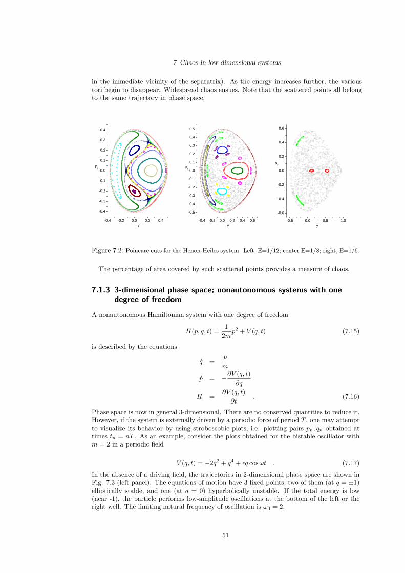
7 Chaos in low dimensional systems
in the immediate vicinity of the separatrix). As the energy increases further, the varioustori begin to disappear. Widespread chaos ensues. Note that the scattered points all belongto the same trajectory in phase space.
-0.4 -0.2 0.0 0.2 0.4
-0.4
-0.3
-0.2
-0.1
0.0
0.1
0.2
0.3
0.4
py
y-0.4 -0.2 0.0 0.2 0.4 0.6
-0.5
-0.4
-0.3
-0.2
-0.1
0.0
0.1
0.2
0.3
0.4
0.5
py
y-0.5 0.0 0.5 1.0
-0.6
-0.4
-0.2
0.0
0.2
0.4
0.6
py
y
Figure 7.2: Poincare cuts for the Henon-Heiles system. Left, E=1/12; center E=1/8; right, E=1/6.
The percentage of area covered by such scattered points provides a measure of chaos.
7.1.3 3-dimensional phase space; nonautonomous systems with onedegree of freedom
A nonautonomous Hamiltonian system with one degree of freedom
H(p, q, t) =1
2mp2 + V (q, t) (7.15)
is described by the equations
q =p
m
p = −∂V (q, t)∂q
H =∂V (q, t)
∂t. (7.16)
Phase space is now in general 3-dimensional. There are no conserved quantities to reduce it.However, if the system is externally driven by a periodic force of period T , one may attemptto visualize its behavior by using stroboscobic plots, i.e. plotting pairs pn, qn obtained attimes tn = nT . As an example, consider the plots obtained for the bistable oscillator withm = 2 in a periodic field
V (q, t) = −2q2 + q4 + εq cos ωt . (7.17)
In the absence of a driving field, the trajectories in 2-dimensional phase space are shown inFig. 7.3 (left panel). The equations of motion have 3 fixed points, two of them (at q = ±1)elliptically stable, and one (at q = 0) hyperbolically unstable. If the total energy is low(near -1), the particle performs low-amplitude oscillations at the bottom of the left or theright well. The limiting natural frequency of oscillation is ω0 = 2.
51

7 Chaos in low dimensional systems
The other two panels of Fig. 7.3 show what happens when a periodically varying field isturned on. The frequency of the field ω = 1.92 is chosen to lie near ω0. At low amplitudesof the driving field and reasonably low energies, a stroboscopic plot of motion is not funda-mentally different from the corresponding plot at the conservative limit ε = 0; the particlestays confined near the top of the potential well. As the driving amplitude increases, theparticle escapes the well and performs a chaotic motion in the vicinity of the separatrix ofthe conservative limit (right panel).
-1 0 1
-2
-1
0
1
2
p
x
-1.0-0.5000.501.01.52.02.0
-1 0 1
-2
-1
0
1
2
p
x
ϖ=1.92ε=0.01
-1 0 1
-2
-1
0
1
2
p
x
ϖ=1.92ε=0.1
Figure 7.3: Stroboscobic plot of the dynamics of (7.17) for ω = 1.92 and 0 < t < 2000 (after
[13]). The left panel shows the contours of phase space trajectories of the unperturbed,
conservative system; note the separatrix at E = 0, which separates bounded from
unbounded motion. Initial conditions were p = 0 and q = 0.24, corresponding to
E = −0.112, an energy near the top of the potential well. The middle panel, at
ε = 0.01, shows that the particle remains trapped in the well. The right panel, at
ε = 0.1, illustrates the escape from the well, and the “breaking of the torus” which
occurs near the separatrix.
7.2 Small denominators revisited: KAM theorem
Recall there was a problem of small denominators; if you start with an integrable Hamilto-nian H0(J1, J2) and functionally independent frequencies ωi = ∂H0/∂Ji and perturb it witha small perturbation µH1(J1, J2, θ1, θ2) then Poincare showed that there are no analytic in-variants of the perturbed system H0 +µH1. Is chaos inevitable? The answer is more or lessyes. Is chaos imminent and overwhelming, even for a small perturbation? The answer is no -as we have seen from circumstantial evidence in the Henon-Heiles Hamiltonian. Kolmogorov,Arnold and Moser (KAM) showed that, if the Hessian of the unperturbed Hamiltonian isnondegenerate, i.e.
det(
∂2H0
∂Ji∂Jj
)= det
(∂ωi
∂Jj
)6= 0 , (7.18)
a torus of the H0 Hamiltonian with frequencies ωi survives, slightly deformed, in the per-turbed system, provided
|n1ω1 + n2ω2| ≥ K(ε)||n1|+ |n2||α ∀ n1, n2 (7.19)
where α > 2 and K(ε) depend on the particulars of the problem. Tori which do not fulfillthis condition may break up. The destroyed tori constitute a dense set. Yet they have avery small measure. Most tori survive. It is possible to understand this using an analogy
52

7 Chaos in low dimensional systems
with the length obtained by excluding from the line continuum a small neighborhood, sayε/n3, around every rational number m/n (recall that the rationals form a dense set). Themeasure of the continuum deleted is
∞∑n=1
n∑m=1
ε
n3=
∞∑n
ε
n2=
π2
6ε . (7.20)
Although irrationals do not form a dense set, they make most of the measure of real numbers.In this sense, almost all tori survive the addition of a small (in practice: even a moderatelylarge) perturbation. Eventually however, as the perturbation grows, chaos ensues.
Note I have used the language of systems with two degrees of freedom just for simplicity.In fact, the KAM theorem holds for an arbitrary number of degrees of freedom, under theconditions described above.
7.3 Chaos in area preserving maps
7.3.1 Twist maps
The twist map allows direct visualization of a Hamiltonian system with two degrees of free-dom, moving on a torus. Let J1, J2 be the action coordinates, and θ1, θ2 the correspondingangle coordinates. Make a Poincare cut each time θ2 = 0 mod 2π. This will by definition beevery τ = 2π/ω2 seconds, where ω2 = ∂H0/∂J2. Then plot the coordinates ρ =
√2J1 and
φ = θ1 on a plane. The points will lie on a circle. I can express the successive values of theangle coordinate on the cut by the sequence
φn+1 = φn + ω1τ
or, more generally, in terms of the winding number w = ω1/ω2
ρn+1 = ρn
φn+1 = φn + 2πw(ρn) (7.21)
where I have explicitly allowed all possible J1’s and hence all possible radii. For a givenenergy this fixes J2, so that the winding number is only a function of ρ. In shorthandnotation this will be (
ρn+1
φn+1
)= T0
(ρn
φn
), (7.22)
where T0 stands for the unperturbed twist map.
Now if the winding number can be expressed as a rational fraction r/s, the cut will becomposed of s points (s-cycle). If not, we have quasiperiodic motion; the cut fills the circledensely.
We would like to find out what happens under a perturbation. This is described below(Poincare-Birkhoff theorem). For the moment, let me just describe what a perturbed mapwill look like - and how to get it. In general,
ρn+1 = ρn + εf1(ρn, φn)φn+1 = φn + 2πw(ρn) + εf2(ρn, φn) (7.23)
where I must choose the functions f1 and f2 such that the map represents a Hamiltonian flow,i.e. it should be a canonical transformation. This can be achieved by using an appropriate
53
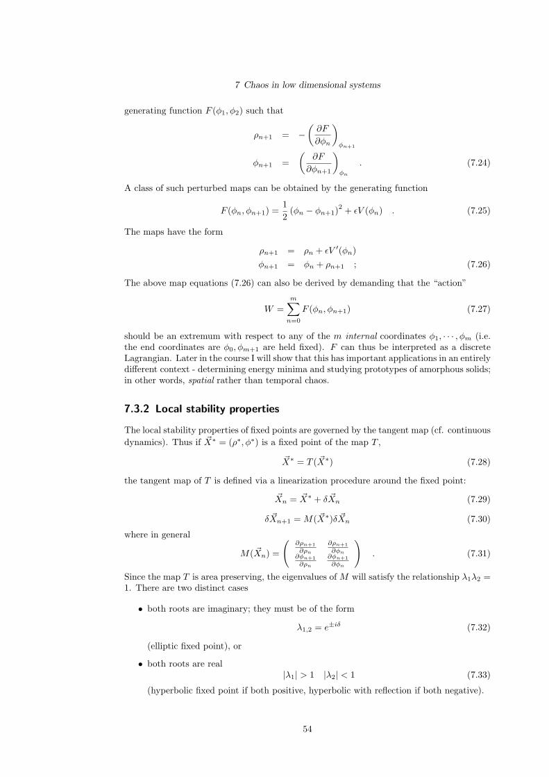
7 Chaos in low dimensional systems
generating function F (φ1, φ2) such that
ρn+1 = −(
∂F
∂φn
)
φn+1
φn+1 =(
∂F
∂φn+1
)
φn
. (7.24)
A class of such perturbed maps can be obtained by the generating function
F (φn, φn+1) =12
(φn − φn+1)2 + εV (φn) . (7.25)
The maps have the form
ρn+1 = ρn + εV ′(φn)φn+1 = φn + ρn+1 ; (7.26)
The above map equations (7.26) can also be derived by demanding that the “action”
W =m∑
n=0
F (φn, φn+1) (7.27)
should be an extremum with respect to any of the m internal coordinates φ1, · · · , φm (i.e.the end coordinates are φ0, φm+1 are held fixed). F can thus be interpreted as a discreteLagrangian. Later in the course I will show that this has important applications in an entirelydifferent context - determining energy minima and studying prototypes of amorphous solids;in other words, spatial rather than temporal chaos.
7.3.2 Local stability properties
The local stability properties of fixed points are governed by the tangent map (cf. continuousdynamics). Thus if ~X∗ = (ρ∗, φ∗) is a fixed point of the map T ,
~X∗ = T ( ~X∗) (7.28)
the tangent map of T is defined via a linearization procedure around the fixed point:
~Xn = ~X∗ + δ ~Xn (7.29)
δ ~Xn+1 = M( ~X∗)δ ~Xn (7.30)
where in general
M( ~Xn) =
(∂ρn+1∂ρn
∂ρn+1∂φn
∂φn+1∂ρn
∂φn+1∂φn
). (7.31)
Since the map T is area preserving, the eigenvalues of M will satisfy the relationship λ1λ2 =1. There are two distinct cases
• both roots are imaginary; they must be of the form
λ1,2 = e±iδ (7.32)
(elliptic fixed point), or
• both roots are real|λ1| > 1 |λ2| < 1 (7.33)
(hyperbolic fixed point if both positive, hyperbolic with reflection if both negative).
54

7 Chaos in low dimensional systems
Periodic motion (s− cycles in the form ~X∗1 , ~X∗
2 , · · · , ~X∗s ) is represented by fixed points of
the T s map,~X∗
j = T s( ~X∗j ) j = 1, 2, · · · , s . (7.34)
The stability of the s-cycle (7.34) is governed by the eigenvalues of the product matrix
M (s) = M( ~X∗s )M( ~X∗
s−1) · · ·M( ~X∗1 ) .
Note that, since the determinant of each one of the terms in the above product is unity,detM (s) = 1. The classification of stability properties is therefore exactly the same (ellipticvs hyperbolic cycles) as in the case of fixed points (cf. above).
7.3.3 Poincare-Birkhoff theorem
The unperturbed twist map with a rational winding number w = r/s will generate an s-cyclewhose points lie on a circle C. This will happen no matter where one starts on the circle.In this sense, every point the circle will be a fixed point of the unperturbed T s
o map,
T so C = C . (7.35)
Note that this differs from the generic situation of an irrational winding number; the circlewith a radius which corresponds to an irrational winding number maps onto itself - but itspoints are not fixed points of any finite repeated application of the map. What happensunder the influence of a perturbation? In order to see this, consider two neighboring circles,C+, with a slightly larger, irrational winding number w+, and C− with a slightly smaller,irrational winding number w−. Under application of the same unperturbed twist map, C+
will be slightly twisted - with respect to C -in the positive (counterclockwise) direction, sincew+ > w; similarly C− will be slightly twisted in the negative (clockwise) direction, sincew− < w. These relative opposite twists of the circles survive under the perturbed twistmap T s
ε - although their form may be distorted. By a continuity argument it is possibleto construct a “zero twist” curve R. If I now apply the map T s
ε to R, the resulting curvewill be distorted with respect to R only in the radial direction (zero twist). Because themap is area preserving, there should, in general, be an even number of intersections, 2ks(exceptions are possible in cases where the curve T s
ε R might tangentially touch the curveR). These intersections are the only fixed points which survive from the original invariantcircle C in the presence of a perturbation. Of the 2ks fixed points, half are elliptically stableand half hyperbolically unstable; elliptic and hyperbolic fixed points come in pairs and theyalternate. This is the Poincare-Birkhoff theorem.
7.3.4 Chaos diagnostics
Power spectra
Given a suitably averaged time-dependent quantity f(t), it is possible to define its powerspectrum
I(ω) =12π
∫ ∞
−∞dteiωtf(t) . (7.36)
If the “signal” is periodic in time, i.e. if f(t) = f(t + T ), it is possible to express it as aFourier series
f(t) =∞∑
n=−∞αne−inΩt (7.37)
55

7 Chaos in low dimensional systems
Figure 7.4: Illustration of the Poincare-Birkhoff theorem. (a) upper left: the unperturbed map:
a circle C with a rational winding number w, along with neighboring circles C+, C−
with irrational winding numbers w+(positive twist), w− (negative twist). (b) upper
right: the perturbed map; outer and inner curve represent, respectively, the slightly
deformed versions of C+, C−. The intermediate curve R is a zero-twist curve obtained
by the requirement of continuity. (c) lower right: tR(continuous curve) and its T sε map
(dashed curve). In this case s = 2. There is no twist under the action of the map,
just pulling and pushing along the radial direction. There is a total of 4 intersections,
corresponding to a stable and an unstable 2-cycle. Following the arrows, it is possible
to determine which points are elliptic and which are hyperbolic. Note that the small
arrows outside R are all pointing in the outward direction (positive twist), and those
inside R in the negative direction (negative twist). (d) a more abstract view of the
elliptic and hyperbolic 2-cycles.
where Ω = 2π/T . It follows that the spectrum
I(ω) =∞∑
n=−∞αnδ(ω − nΩ) (7.38)
will be composed of a series of δ-peaks situated at the fundamental frequency and its higherharmonics.
One can generalize this to the case of a multiply periodic motion - which would be moreapt to describe motion on on a torus. In this case of a doubly periodic motion f(t) is
56

7 Chaos in low dimensional systems
described by a double Fourier expansion
f(t) =∞∑
n1=−∞
∞∑n2=−∞
αn1,n2e−i(n1Ω1+n2Ω2)t (7.39)
and the spectrum
I(ω) =∞∑
n1=−∞
∞∑n2=−∞
αn1,n2δ(ω − n1Ω1 − n2Ω2) , (7.40)
forms peaks at all sum and difference frequencies. Under ideal conditions (cf. Fig. 7.5) it
0.0 0.1 0.2 0.3 0.410-8
10-7
10-6
1x10⁻⁵
ϖ/2π
Pow
er s
pect
ra
0.0 0.1 0.2 0.3 0.410-8
10-7
10-6
1x10⁻⁵
1x10⁻⁴
ϖ/2π
Pow
er s
pect
ra
0.0 0.1 0.2 0.3 0.410-8
10-7
10-6
1x10⁻⁵
ϖ/2π
Pow
er s
pect
ra
Figure 7.5: Power spectra of py(t) for quasiperiodic (left and center panels) and chaotic (right
panel) trajectories of the Henon-Heiles system at energy E = 1/8. In the case of
quasiperiodic motion (left) it is possible to make a detailed identification of the five
peaks in terms of two fundamental torus frequencies at f1 = 0.16 and f2 = 0.12, their
second harmonics, and the difference f1 − f2 = 0.04. A similar assignment can be
made in the case of the center panel. Chaotic spectra (right panel) are characterized
by broader, noisier features.
should of course be possible to distinguish regularity from chaos by its spectral signatures.In the former case the spectrum is periodic or quasiperiodic, in the latter case there isa lot of noise, perhaps accompanied by broad peaks. In practice however, the intrinsiclimitations of obtaining useful power spectra from finite numerical (or experimental) data,renders spectral information somewhat limited as a sole criterion of deciding whether a givenprocess is chaotic or not.
Lyapunov exponents
Lyapunov exponents quantify the usual defining property of deterministic chaos, which isthe sensitive dependence on initial conditions. Consider a certain trajectory of the - notnecessarily area-preserving - N -dimensional map T
~Xj+1 = T ( ~Xj) j = 0, · · ·n− 1, (7.41)
and a “neighboring” trajectory, which starts at ~X0 + δ ~X0. The difference between the twotrajectories after the first iteration can be expressed in terms of the tangent map:
δ ~X1 = M( ~X0)δ ~X0 ;
57

7 Chaos in low dimensional systems
after the second iteration it will be
δ ~X2 = M( ~X1)δ ~X1 = M( ~X1)M( ~X0)δ ~X0 ,
and after n iterations
δ ~Xn = M( ~Xn−1)M( ~Xn−2) · · ·M( ~X0)δ ~X0
= Λn( ~X0, · · · , ~Xn−1)δ ~X0 , (7.42)
where the N ×N matrix Λ is the nth root of the product of all n tangent maps involved inthe trajectory; in general, Λ will have N eigenvalues λα(n), α = 1, · · ·N , which will dependon the order of iteration n. The Lyapunov exponents are defined as
σi = limn→∞
ln |λα(n)| α = 1, · · · , N. (7.43)
Note that in general there are as many Lyapunov exponents as the dimensionality of themap. If the map is area preserving, they come in pairs, i.e. for each positive exponent, anegative exponent with the same magnitude must occur. This corresponds to expandingand shrinking directions; It is obvious from (7.42) that, if we order Lyapunov exponents indecreasing order
σ1 > σ2 > · · ·σN (7.44)
the largest (positive) exponent will eventually dominate the right hand side of (7.42). Thiswill happen even if there is a vanishingly small component of δ ~X0 in the direction of theeigenvector of Λ which corresponds to σ1. The norm ||δ ~Xn|| will grow exponentially aseσ1n. This is exactly the physical content of “sensitive dependence on initial conditions”.Lyapunov exponents provide a measure of just how sensitive this dependence is.
Note: here I have defined Lyapunov exponents in the context of maps. If time permits, Iwill present the definitions - and computational procedures - for dynamical systems governedby differential equations, i.e. Hamiltonian or dissipative dynamics.
7.3.5 The standard map
kicked pendulum, kicked rotator
Consider the nonautonomous Hamiltonian system defined by a kicked pendulum, wheregravity acts in bursts, every τ seconds:
H =p2
2− K
(2π)2cos(2πq)
∞∑n=−∞
δ(t− nτ) (7.45)
where p is the angular momentum and 2πq the angle, referred to the perpendicular direction(cf. H-atom in electric field.)
The equations of motion are
p = −∂H
∂q= −K
2πsin(2πq)
∞∑n=−∞
δ(t− nτ)
q =∂H
∂p.
The first equation implies that p is constant, except at times t = nτ , when it changes by adiscrete step. Defining
pn = limε→0
p(nτ − ε) ,
58

7 Chaos in low dimensional systems
I can integrate in the neighborhood of t = nτ , set τ = 1 and obtain what is known as thestandard map
pn+1 = pn − K
2πsin(2πqn)
qn+1 = qn + pn+1 . (7.46)
Eqs. 7.46 belong to the general class (7.26) of area preserving twist maps. In the following,the coordinates pn, qn will be understood as mod1, unless stated otherwise.
Fixed points
The map (7.46) has two fixed points:
• p∗ = 0, q∗ = 0, which is elliptic, and
• p∗ = 0, q∗ = 1/2, which is hyperbolic .
(NB: the published literature has adopted a variety of conventions; one of them has a differentsign in the Hamiltonian; this amounts to a shift of q by 1/2)
Summary of results
At small values of K (cf. Fig. 7.6) there is no sign of chaos. We observe the tori whichsurround the elliptic fixed point, which extend up to the separatrix which leaves off the hy-perbolic fixed point. Furthermore, we observe a large number of “horizontal” tori - meaningthat they run all the way from left to right; these tori are the slightly deformed versionsof the original irrational tori of the unperturbed system, which have survived the pertur-bation. Finally, the structure which emanates from the period 2 cycle, around the centerof the picture, is visible. This resonant torus is broken; according to the Poincare-Birkhofftheory, we observe a period 2 island chain, and the hyperbolic fixed points nested betweenthem.
0.0 0.2 0.4 0.6 0.8 1.00.0
0.2
0.4
0.6
0.8
1.0
p
q
K=0.5
0.0 0.2 0.4 0.6 0.8 1.00.0
0.2
0.4
0.6
0.8
1.0
p
q
K=0.8
Figure 7.6: Trajectories of the standard map at K = 0.5 (left panel), K = 0.8 (right panel).
As the perturbation increases, more and more near-resonant horizontal tori break up.Chaos develops around the separatrices of the leading resonances (hyperbolic fixed point
59

7 Chaos in low dimensional systems
0.0 0.2 0.4 0.6 0.8 1.00.0
0.2
0.4
0.6
0.8
1.0
p
q
K=0.9716354
0.0 0.2 0.4 0.6 0.8 1.00.0
0.2
0.4
0.6
0.8
1.0
p
q
K=1.1716354
Figure 7.7: Trajectories of the standard map at K = Kc = 0.9716354 (left panel), K = 1.17 (right
panel).
and in the crossings between period 2 island chain). The survival of a torus depends on“how irrational”- its winding number is. In order to see what this means, look at thecontinued fraction representation of an irrational number
w = a0 +1
a1 + 1a2+···
≡ a0; a1, a2, · · · , (7.47)
where the integers ai satisfy a0 ≥ 0 and ai > 1 ∀i ≥ 1. An n-th order approximationw = rn/sn can be generated by the sequence
rn = anrn−1 + rn−2
sn = ansn−1 + sn−2 (7.48)
with r−2 = 0, r−1 = 1, s−2 = 1, s−1 = 0.
Eq. (7.48) implies thatsn+1 > an+1sn . (7.49)
It follows that|w − rn
sn| < 1
snsn+1<
1an+1s2
n
. (7.50)
Thus, if an+1 is large, the nth approximation is a good one. An example is
π = 3; 7, 15, 1, 292, · · ·which leads to π = 3.14159265 · · · ≈ r3/s3 = 355/113 = 3.14159292, good to 7 digits.Conversely, the representation
√2 = 1; 2, 2, 2, 2, · · ·
leads to√
2 = 1.414213 · · · ≈ r3/s3 = 17/12 = 1.41666 · · ·, which has an error in the 4thdigit. In this sense, the golden mean
√5 + 12
= 1; 1, 1, 1, 1, · · · (7.51)
and its inverse √5− 12
= 0; 1, 1, 1, 1, · · · (7.52)
60

7 Chaos in low dimensional systems
can be considered as the “most irrational” numbers. Therefore, the non-resonant torus witha winding number equal to the inverse golden mean, is expected to be the last to break.
The disappearance of the last, “golden mean” torus at K = Kc = 0.9716354 (cf. Fig.7.7, left panel)is a key event in the nonlinear scenario. It signals the transition from localto widespread chaos. The following aspects deserve special attention:
• breaking of analyticity: As K approaches the critical value Kc, the deformation of thetorus increases dramatically. The following procedure [14] makes it possible to followthe torus’ shape and detailed properties. First observe, following Greene [15], thatan instability of a torus with irrational winding number w can be associated with theinstability of an sn →∞ cycle, where sn is defined in terms of the sequence rn/sn usedto approximate w. Thus, rather that try to construct a torus directly, it is possible todetermine successive cycles and their thresholds of instability.
It useful to introduce the Moser representation (parametrization) [14]
qj = tj + u(tj) , (7.53)
appropriate to any cycle with a rational winding number w; here tj = jw = jr/s. Theproperty qj = qj+s implies
u(tj) = u(tj + 1) mod 1 . (7.54)
Note that the periodic function u(t) - which can be shown to be odd - is only definedon a rational set t = tj = jr/s, but this set becomes more and populous as s isincreased. Fig. 7.8 shows the dependence of u(t), evaluated for an s = 4181 cyclewhich approximates the torus with a golden mean winding number, as a function ofK. Note how the function becomes less and less smooth as Kc is approached.
• self similarity: Fig. 7.8 shows the shape of the KAM golden-mean torus at two non-critical K’s and at K = Kc. Note the detailed view of the non-smooth function.The detailed numerics [14] allows the conjecture of self-similarity; in other words, thevalleys and hills of the curve repeat themselves at all possible scales of numerical ob-servation. In this sense, KAM torus disappearance resembles a critical phenomenon.Self-similarity is very well demonstrated in the frequency spectra. The odd functionu(t) can be represented in a Fourier series
u(t) =∞∑
f=1
Af sin 2πft
The product fAf is shown in Fig. 7.9 as a function of f , for the same values of K asin Fig. 7.8. Note the presence of more and more peaks as the critical value of K isapproached. At K = Kc self similar behavior occurs, with primary peaks occurring atthe Fibonacci numbers.
• Arnold diffusion: A picture of the widespread chaos which occurs at higher valuesof the nonlinear parameter K > Kc is given in Fig. 7.7) (right panel). Unless apoint starts in the immediate neighborhood of the elliptic fixed point, or the veryfew islands, it will typically generate a chaotic orbit which may diffuse over a largetwo-dimensional area of phase space. This diffusive behavior can be quantitativelycharacterized as follows.
Suppose we relax the mod 1 condition on the momentum p in (7.46). In other wordswe allow the phase space to be a cylinder of perimeter 1 and look at the quantity
D = limn→∞
[(pj+n − pn)2
2n
], (7.55)
61

7 Chaos in low dimensional systems
0.0 0.2 0.4 0.6 0.8 1.0
0.55
0.60
0.65
0.70
p
q
0.337 0.338 0.339 0.340
0.676910
0.676912
0.676914
p
q
0.674534
0.674536
0.674538
0.0 0.1 0.2 0.3 0.4 0.50.00
0.02
0.04
0.06
0.120 0.125 0.130
0.0460
0.0465
u
t
Figure 7.8: The torus with a winding number approximately equal to the inverse of the golden
mean W ∗ = (√
5 − 1)/2, at K = 0.5, 0.9, Kc. The curves shown are actually sets of
discrete points belonging to cycles of order s = 4181 with a rational winding number
w = r/s = 2584/4181 which differs from W ∗ by less than 3 × 10⁻⁸. I. Left panel: the
torus in the (p, q) plane. II. Center panel: a detailed view of the same torus in the
cases K = .9 (right y-scale) and K = Kc (left y-scale). III. Right panel: the function
u(t) which describes the torus of the standard map in parametric form. Again, the
curve shown is actually obtained from an 4181-cycle which approximates the irrational
winding number W ∗. Note how the function changes from smooth at K = 0.5, to
somewhat bumpy at K = 0.9, to very bumpy at K = Kc. The inset shows a detailed
view of the critical curve, which suggests self-similar behavior (After [14]).
2 8 32 128 512 20480.00
0.01
0.02
0.03
0.04
0.05
f|A(f)|
f
2 8 32 128 512 20480.00
0.01
0.02
0.03
0.04
0.05
f|A(f)|
f
2 8 32 128 512 20480.00
0.01
0.02
0.03
0.04
0.05
f|A(f)|
f
Figure 7.9: Fourier coefficients of the function u(t), which describes parametrically the torus with
with a golden mean winding number, at K = 0.5, 0.9, Kc. The quantity plotted is
f |Af |. The curve at K = Kc (right panel), with primary contributions at the Fibonacci
numbers, suggests self-similar behavior (after [14]).
which describes the coefficient of diffusion in momentum space.
As long as K < Kc, the existence of even a single torus presents a topological barrierto diffusion1. D should vanish.
1this is no more the case in higher dimensions! Arnold diffusion is generic in higher dimensionality becausetori can be bypassed.
62

7 Chaos in low dimensional systems
In the opposite limit K À Kc, we can estimate the diffusion coefficient as follows.From (7.46)
pj+n = pj − K
2π
j+n−1∑
l=j
sin(2πql) (7.56)
and hence
(pj+n − pj)2 =(
K
2π
)2 j+n−1∑
l,l′=j
sin(2πql) sin(2πql′) . (7.57)
Now, since qj+1 = qj + pj+1 mod 1, if pj+1 is large, qj+1 is essentially random, i.e.uncorrelated to qj . The only correlations which survive are from terms l′ = l. Onthe average, the double sum will therefore be equal to n/2 (the 1/2 factor from theaverage value of sin2). Therefore
D ≈(
K
4π
)2
if K À Kc . (7.58)
In the case where K slightly exceeds Kc, Chirikov has estimated
D ∝ (K −Kc)2.56
. (7.59)
• Cantori: (7.59) makes clear that, even beyond the stochasticity threshold, diffusiondoes not proceed uninhibited. At values slightly above Kc the diffusion constant is infact very close to zero. It appears that some barriers to diffusion persist after all KAMtori have been broken.
Resistance to diffusion can be related to a particular class of orbits with irrationalwinding numbers, which do not fully cover a one-dimensional curve (Fig. 7.10), butleave a countable set of open intervals empty - i.e. they form a Cantor set. Because ofthis property they were named cantori by Percival. The existence of cantori as isolatedregular orbits embedded in a sea of chaos is remarkable. We will deal with them againin Chapter 9, in the context of solid state theory.
An excellent review of the transport properties of Hamiltonian maps has been writtenby Meiss [16].
7.3.6 The Arnold cat map
The area preserving map
xn+1 = xn + yn mod 1yn+1 = xn + 2yn mod 1 (7.60)
has a tangent map
M =(
1 11 2
)(7.61)
which does not depend on the coordinates. The eigenvalues of the map are
λ1,2 =12
(3±
√5)
(7.62)
and the Lyapunov exponents σ1 = ln λ1 = −σ2. There is a single, hyperbolic fixed pointat x∗ = y∗ = 0. Neighboring trajectories everywhere diverge exponentially. All cycles areunstable. What happens to a cat thus mapped is shown in Fig. 7.11.
63
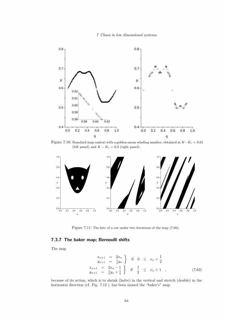
7 Chaos in low dimensional systems
0.0 0.2 0.4 0.6 0.8 1.00.4
0.5
0.6
0.7
0.8
0.58 0.60 0.620.58
0.59
0.60
0.61
0.62
p
q
0.0 0.2 0.4 0.6 0.8 1.00.4
0.5
0.6
0.7
0.8
p
q
Figure 7.10: Standard map cantori with a golden-mean winding number, obtained at K−Kc = 0.01
(left panel) and K −Kc = 0.3 (right panel).
0.0 0.2 0.4 0.6 0.8 1.00.0
0.2
0.4
0.6
0.8
1.0
y
x
0.0 0.2 0.4 0.6 0.8 1.00.0
0.2
0.4
0.6
0.8
1.0
y
x
0.0 0.2 0.4 0.6 0.8 1.00.0
0.2
0.4
0.6
0.8
1.0
y
x
Figure 7.11: The fate of a cat under two iterations of the map (7.60).
7.3.7 The baker map; Bernoulli shifts
The map
xn+1 = 2xn
yn+1 = 12yn
if 0 ≤ xn <
12
xn+1 = 2xn − 1yn+1 = 1
2yn + 12
if
12
≤ xn < 1 , (7.63)
because of its action, which is to shrink (halve) in the vertical and stretch (double) in thehorizontal direction (cf. Fig. 7.12 ), has been named the “baker’s” map.
64

7 Chaos in low dimensional systems
0.0 0.2 0.4 0.6 0.8 1.00.0
0.2
0.4
0.6
0.8
1.0
y
x
0.0 0.2 0.4 0.6 0.8 1.00.0
0.2
0.4
0.6
0.8
1.0
y
x
0.0 0.2 0.4 0.6 0.8 1.00.0
0.2
0.4
0.6
0.8
1.0
y
x
Figure 7.12: Evolution of the cat of Fig. 7.11 under three successive iterations of the baker’s map
(7.63).
• the map is fully reversible.
• just like the cat map, the baker’s map has a single, hyperbolic fixed point at x∗ =y∗ = 0.
• the tangent map is the same for any trajectory:
M =(
2 00 1/2
)(7.64)
does not depend on the coordinates. The eigenvalues of the map are λ1 = 2; λ2 = 1/2and the corresponding Lyapunov exponents σ1 = ln 2 = −σ2.
• mixing: The map has the mixing property.
• Bernoulli shifts: Let x0, y0 be represented in binary notation as
x0 = .a1a2 · · · ai · · ·y0 = .b1b2 · · · bi · · · (7.65)
where ai, bi = 0 or 1. A symbolic “back-to-back” representation of both coordinatescan be written as
X0 = (x0, y0) = · · · bi · · · b2b1.a1a2 · · · ai · · · . (7.66)
The first iteration, by doubling the x and halving the y produces
X1 = (x1, y1) = · · · bi · · · b2b1a1.a2 · · · ai · · · . (7.67)
i.e. shifts the decimal point by one position to the right.2 This process is called aBernoulli shift.Now look at a “coarse-grained” description of the sequence Xn mod 1, where theonly information retained is the first digit after the decimal point. For typical (i.e.irrational) x0, y0 this will be an aperiodic sequence of zeros and ones, i.e. a sequencewhich is essentially equivalent to the tossing of a coin. Note that this totally randombehavior has been obtained by coarse-graining of an entirely deterministic, reversiblemap. I will return to Bernoulli shifts in the next section, because they are a generalfeature of deterministic chaos.
2Convince yourselves that this is so by looking separately at the cases a1 = 0 and a1 = 1!
65

7 Chaos in low dimensional systems
7.3.8 The circle map. Frequency locking
The circle mapθn+1 = θn + Ω−K sin θn (7.68)
is a one-dimensional non-area-preserving map; I introduce it here in order to describe theprinciple behind frequency locking. In addition, the map exhibits KAM characteristics,breaking of rational tori etc (Arnold).
I will look at the winding number
R =12π
limn→∞
(θn − θ0
n
). (7.69)
In the integrable limit, K = 0, θn − θ0 = nw and therefore R = Ω. For K 6= 0
∂θn+1
∂θn= 1−K cos θn 6= 1 (7.70)
-2 0 2
-1
0
1
2
A''
A'AΩ/K
θ
Figure 7.13: Tangent bifurcation scheme for the fixed point of Eq. (7.71).
Consider first the fixed point, θn = θ∗ ∀n, corresponding to R = 0. From (7.68), thiswill happen if
Ω−K sin θ∗ = 0 . (7.71)
Eq. 7.71 has no solutions if |Ω| > K, two solutions if |Ω| < K (one corresponding to astable and the other to an unstable fixed point), and one solution if |Ω| = K. This behaviorcorresponds to a tangent bifurcation scenario (cf. Fig. 7.13 ). Note that the winding numberR will now be equal to zero not just for Ω = 0, but for any Ω < K.
An analogous situation occurs for R = 1/2, i.e. for a 2-cycle. In that case, the 2-cycleremains stable within a band Ω−1/2 < Ω < Ω+
1/2, where Ω±1/2 = π±K2/4, i.e. the band widthis ∆Ω1/2 = K2/2. More generally, a rational winding number R = P/Q will “lock in”tothat value for any Ω within a band of bandwidth
∆ΩP/Q ∝ KQ . (7.72)
This is the phenomenon of frequency locking. The total length of frequency locked intervalstends to zero as K → 0. Note the analogy with the breaking of KAM-tori (Arnold); irrationalwinding numbers occupy most of available phase space in the slightly perturbed system.Stable frequency-locked intervals in the Ω−K plane are shown in Fig. 7.14
For values K < 1 the winding number R will therefore exhibit frequency-locking stepsat various rational values of R; between those steps, there will be intervals where R will
66

7 Chaos in low dimensional systems
Figure 7.14: Frequency locking in the circle map. For any value of K > 0 there is a small band
of Ω values, of width ∆ΩP/Q, for which the winding number R locks to the rational
value P/Q. As long as K < 1, the total measure of such intervals is less than 1. At
K = 1, the total measure of locked-in frequency intervals is equal to unity. At values
K > 1, bands corresponding to different rational ratios begin to overlap (resonance
overlap). This is indicated by the dotted lines (from [17]).
Figure 7.15: The complete devil’s staircase at K = 1. Frequency locking takes place at all ra-
tionals.The inset shows that the staircase exhibits self-similarity at all scales (from
[17]).
depend linearly on Ω. This kind of behavior is represented pictorially by the “incompletedevil’s staircase”. At K = 1 there are steps at all rational numbers and no portions with afinite slope. Frequency-locked intervals now have measure 1. This is the “complete devil’sstaircase” (Fig. 7.15). For values K > 1 chaos occurs as the resonance regions depicted inFig. 7.14 begin to overlap. More details in [17].
7.4 Topology of chaos: stable and unstable manifolds,homoclinic points
The stable manifold of a cycle3 is the set of points such if the forward map is started fromone of them, further iterates will approach the cycle. Similarly, in the case of an invertiblemap, the unstable manifold of a cycle is the set of points such if the inverse (backward) mapis started from one of them, further iterates will approach the cycle.
3A fixed point of a map is a cycle of period 1; for systems with continuous dynamics it is straightforwardto generalize statements on cycles and apply them to periodic orbits.
67

7 Chaos in low dimensional systems
Stable and unstable manifolds cannot intersect themselves; however, they can intersecteach other. If the manifolds belong to the same hyperbolic fixed point, their intersectionsare called homoclinic points. If the manifolds belong to different hyperbolic fixed points, theintersections are called heteroclinic points. Fig. 7.16 shows what happens at a homoclinicpoint X0. Let X1, X2 be two successive iterates of the X0 along the stable manifold (s).Consider now the neighboring points Y0 on the unstable manifold (u). Because it is a“predecessors” of X0 (follow the arrows!), its iterate Y1 must find a place on the unstablemanifold prior to X1. In order to accommodate this requirement, the unstable manifold mustfold. Now, as the hyperbolic fixed point P is approached, the distance between iterates alongthe stable manifold decreases. The folds of the unstable manifold must lie closer and closerto each other. Because of the area preserving property (the crossed areas in the figure shouldbe equal), this makes the folds larger and larger in amplitude. Thus, if a single homoclinicpoint exists, an infinite sequence is generated. Fig. 7.16 (right panel) illustrates this in thecase of the hyperbolic fixed point of the standard map.
The complexity of the intersecting stable and unstable manifolds near hyperbolic fixedpoints lies at the heart of chaos in conservative systems. It was aptly recognized by itsdiscoverer, Poincare, with the fitting response “the complexity of this figure will be striking,and I shall not even try to draw it”.
0.47 0.48 0.49 0.50 0.51 0.52-0.01
0.00
0.01
0.02
0.03
p
q
K=0.5
Figure 7.16: Homoclinic points in the vicinity of a hyperbolic fixed point. Left: a schematic view
(cf. text); Right: the stable (red, thicker points) and unstable (black, thinner points)
manifolds of the hyperbolic fixed point of the standard map at a low value of the
nonlinearity parameter K = 0.5.
For more details consult the excellent textbooks available, e.g. by Ott [18] or Tabor [19].
68
8 Solitons in scalar field theories
8.1 Definitions and notation
8.1.1 Lagrangian, continuum field equations
Starting point: classical discrete Lagrangian
L =N∑
i=1
12Iφ2
i −mgl(1− cos φi)− 12K(φi+1 − φi)2
, (8.1)
Physical realization, e.g. coupled torsion pendula. Disks of radius l with moment of inertiaI and an extra mass m on the periphery. Terms represent, respectively:
• rotational kinetic energy
• potential energy of mass in gravitational field
• potential energy of coupling
Other physical realizations: arrays of Josephson junctions, one-dimensional magnets, ...
Equations of motion
Iφi = K(φi+1 + φi−1 − 2φi)−mgl sin φi (8.2)
Continuum approximation
•
φi±1 = φ(xi±1) ≈ φ(xi)± aφ′(xi) +12a2φ′′(xi)
where a is the distance between neighboring disks (lattice constant).
• xi → x (continuum space variable)
leads to
c20
∂2φ
∂x2− ∂2φ
∂t2= ω2
0 sin φ (8.3)
where c20 = Ka2/I, ω2
0 = mgl/I.
The Klein-Gordon class
Eq. 8.3 is a member of the wider class of Klein-Gordon(KG) field equations
c20φxx − φtt = ω2
0V ′(φ) (8.4)
where the on-site potential can be (examples)
69

8 Solitons in scalar field theories
•
V (φ) =12φ2
original Klein-Gordon (linear, QM ca 1930)•
V (φ) =18(1− φ2)2
known as φ4 (displacive phase transitions, continuum version of Ising model)•
V (φ) = 1− cos φ
known as Sine-Gordon (misnomer 1970, rhymes with Klein-Gordon); proposed earlierby Frenkel-Kontorova in context of dislocations, Skyrme in the 60s as a nonlinear fieldmodel for nucleons.
Of interest for characterization of on-site potential: vacuum state, defined by
V ′(φ0) = 0V ′′(φ0) > 0 (8.5)
As defined (dimensionless) all examples have V (φ0) = 0 and V ′′(φ0) = 1. Hence for smalldisplacements from φ0
V (φ− φ0) ≈ 12(φ− φ0)2 .
Note further that the 3 examples defined above have, respectively,
1. a single vacuum
2. two degenerate vacua
3. an infinite number of degenerate vacua.
The field equations (8.4) can also be directly derived from the continuous Lagrangian
L = A
∫dxL
where
L(φ, φx, φt) =12
(∂φ
∂t
)2
− 12c20
(∂φ
∂x
)2
− ω20V (φ)
is the Lagrangian density, and A defines the energy scale. In the SG example, A = I/a.
Symmetries and Conservation laws
Symmetries and conservation laws have been discussed in Section 1.4. In particular, theinvariance of the Lagrangian density with respect to space and time leads, respectively, tothe conservation of total momentum P and energy E. Furthermore, Lorentz invariance leadsto the conservation of angular momentum, which in 1+1 dimensional systems is simply
EX − Pt .
70

8 Solitons in scalar field theories
In the special case of P = 0 (localized field configurations with vanishing total momentum),this implies that the center of energy remains fixed. This is the relativistic analog of thecenter-of-mass theorem of Newtonian dynamics. It turns out to be quite useful in solitondynamics.
Furthermore, Lorentz invariance implies that if φ(x) is a solution of (8.4), so is φ(γ(x−vt)),where γ = (1−v2/c2
0)−1/2 and |v| < c0. In other words, any static solution can be “Lorentz-
boosted”.
8.2 Static localized solutions (general KG class)
8.2.1 General properties
The vacuum
Note that the vacuum (or vacua) is always a solution of the equations of motion (8.4).
Other solutions
I look for static, localized solutions - which may then be Lorentz-boosted. The startingpoint is
c20φxx = ω2
0V ′(φ)
or, in dimensionless form,d2φ
dξ2=
dV
dφ(8.6)
where d = c0/ω0 and ξ = x/d. Multiplying both sides of (8.6) by dφ/dξ, I obtain
12
d
dξ
[(dφ
dξ
)2]
=dV
dξ
which has a first integral
12
(dφ
dξ
)2
= V + const.
For solutions which are localized, i.e.
limξ±∞
dφ
dξ= 0 (8.7)
and
limξ±∞
V = V (φ0) = 0
the integration constant vanishes. A second integral can then be formally written as
ξ − ξ0 = ±∫ φ
φ0
dφ′1√
2V (φ′). (8.8)
71
8 Solitons in scalar field theories
8.2.2 Specific potentials
The linear KG case
In the linear KG case, V (φ) = φ2/2 (8.8) becomes
ξ − ξ0 = ±∫ φ
dφ′1φ′
= ± ln φ
or
φ = e±(ξ−ξ0)
which, although it formally satisfies the original field equation, is not a localized solution inthe sense of (8.7). Therefore it is not a physical solution.
The φ4 kink
In the φ4 case (8.8) becomes
ξ − ξ0 = ±∫ φ
dφ′1
12 (1− φ′ 2)
= ±2 arctanh φ
or
φK(x) = ± tanh(
x− x0
2d
), (8.9)
where x0 = ξ0d . The upper sign corresponds to a kink, the lower to an antikink. Bothsolutions interpolate between the two degenerate vacua.
The SG kink
In the SG case (8.8) becomes
ξ − ξ0 = ±∫ φ
dφ′1√
2(1− cosφ′)
= ±∫ φ
dφ′1
2 sin φ′2
= ln tanφ
4
or
φK(x) = 4 arctan exp±x− c0t− x0
d . (8.10)
The solution with the upper sign interpolates between φ0 = 0 and φ0 = 2π, the one withthe lower sign conversely.
72

8 Solitons in scalar field theories
8.2.3 Intrinsic Properties of kinks
Topological charge
Kinks (and antikinks) interpolate between distinct, degenerate vacua. They are known astopological solitons. The conserved quantity
Q =∫ ∞
−∞dx
dφ
dx= φ(∞)− φ(−∞) (8.11)
is known as topological charge. A φ4 kink has topological charge 1, an antikink −1. A SGkink has topological charge 2π, an antikink −2π.
Rest energy of a kink
The total energy can be obtained from the Hamiltonian density
H = A
12
(∂φ
∂t
)2
+12c20
(∂φ
∂x
)2
+ ω20V (φ)
. (8.12)
For a static kink, the first term is zero, and the second and third terms are equal (cf. above).Thus
EK ≡ Mc20 = Ac2
0
∫ ∞
−∞dx
(∂φ
∂x
)2
= Ac20
1d
∫ ∞
−∞dξ
(∂φ
∂ξ
)2
= Ac20
1d
∫ φ2
φ1
dφ∂φ
∂ξ
or
M =A
d
∫ φ2
φ1
dφ√
2V (φ) . (8.13)
Note that we do not need the explicit form of the kink solution in order to calculate therest mass. In the case of the φ4 field, this gives M = 4A/3d. In the case of the SG field,M = 8A/d.
Energy and momentum of a moving kink: classical wave-particle duality
The energy of the moving kinkφK (γ(x− vt))
whereγ =
1√1− v2
c20
can be directly computed from the full Hamiltonian density. It is
E(v) = Mc20γ . (8.14)
The momentum can be computed from (1.49) and is equal to
P (v) = Mγv . (8.15)
73
8 Solitons in scalar field theories
The energy-momentum relationship
E2 = P 2c20 + M2c4
0
is also satisfied.
The fact that kink and antikink solutions satisfy the usual relativistic kinematic relationswhich ordinarily hold for mass points suggests that these classical localized fields may, formany practical purposes, be effectively treated like particles. The remarkable property ofparticle-wave duality at a classical level suggests that soliton-bearing classical Lagrangiansmight be good candidates for the construction of nonlinear quantum field theories.
8.2.4 Linear stability of kinks
Consider small displacements around a static kink solution of the KG class. The total space-and time-dependent field is written as
φ(x, t) = φK(x) + χ(x, t) (8.16)
where χ will be regarded as a small quantity. Keeping only linear terms in χ leads to
c20χxx − χtt = ω2
0 V ′′(φK) χ .
Using a separation of variables ansatz
χ(x, t) =∑
j
αjeiωjtfj(x) (8.17)
leads to the eigenvalue equation
−d2fj
dξ2+ V ′′(φK)fj(ξ) = Ω2
jfj(ξ) (8.18)
where I have again introduced the dimensionless space variable ξ = x/d, and Ωj = ωj/ω0.
Eq. (8.18) is has the form of a Schrodinger equation. The effective potential is the secondderivative of V , evaluated at φ = φK . Because φK asymptotically approaches the vacuumfield values, the effective potential (Draw!) approaches V ′′(φ0) which with our conventionshas the value 1. Possible eigenstates of (8.18) may then be
• localized (bound), with Ω2 < 1 or
• extended (scattering) states, with Ω2 > 1 .
Linear stability requires thatΩ2
j ≥ 0 . (8.19)
Bound states. The zero frequency (Goldstone) mode
The functionf0 =
dφK
dξ(8.20)
is always an eigenstate of (8.18), associated with the eigenvalue 0. One can see this bynoting that satisfying
−φK,ξξξ + V ′′(φK)φK,ξ = 0
74

8 Solitons in scalar field theories
is equivalent to satisfyingd
dξ[−φK,ξξ + V ′(φK)] = 0.
But the brackets are identically zero for a kink solution.
The zero-frequency (or translational) mode, named after Goldstone, reflects the invarianceof the kink solution under translations. Note in this context that the integration constantξ0 (cf. above) does not enter the expression for the rest-energy. A kink (or antikink) canbe translated in space at zero energy cost. A kink solution centered at zero has the sameenergy with a kink solution centered at α. If α is small, the latter can be obtained from theformer by Taylor expansion
φK(ξ − α) ≈ φK(ξ)− αdφK
dξ
which is why dφK/dξ must be an eigenstate of (8.18).
The Goldstone mode must be the eigenstate with the lowest Ω2j value. One can see this
from the fact that, since kinks are monotonic functions in space, dφK/dξ has no nodes.
Other bound states may or may not exist, depending on the details of the effective po-tential. For example, the SG kink has no further bound states. The φ4 kink has a furtherlocalized mode, with an internal oscillation frequency .... and an eigenfunction ....
Scattering states. Phase shifts
In general, scattering states consist of an incident, a transmitted and a reflected wave.The effective potentials which correspond to both the SG and the φ4 kink have the specialproperty that they are reflectionless. In other words, the eigenfunctions corresponding toextended states with frequencies
Ω2q = 1 + q2 (8.21)
have the asymptotic formlim
x±∞fq(ξ) ∼ eiqξ±iδ(q)/2 . (8.22)
The total phase shift δ(q) describes the net effect of the interaction between an incidentphonon plane wave and a static kink.
Note that the above property is asymptotic. The exact form of extended eigenstates maybe significantly distorted in the neighborhood of the kink. For example, in the SQ case
fq(ξ) = (iq + tanh ξ) eiqξ ,
from whichδ(q) = 2 arctan
1q
follows.
8.3 Special properties of the SG field
8.3.1 The Sine-Gordon breather
The SG field equations admit a family of special localized solutions with an internal oscilla-tion
φbr(x, t) = 4 arctan[ρ
sin ω(t− t0)cosh[(x− x0)/λ]
](8.23)
75

8 Solitons in scalar field theories
-6 -4 -2 0 2 4 6
-3
-2
-1
0
1
2
3
φ
x/d
µ=π/4
-20 -15 -10 -5 0 5 10 15 20-7
-6
-5
-4
-3
-2
-1
0
1
2
3
4
5
6
7
φ
x/d
µ=π/2.001
Figure 8.1: Left: multiple snapshots of a SG breather with intermediate amplitude. Right: a very
slow breather with µ = π/2.001 which looks like a bound kink-antikink pair (of course
if you observe the very slow oscillation over an extremely long period of time you will
note the periodic motion). The snapshots are taken at times which are very far apart
from the point of view of the laboratory observer: ±π/(2ω0 cos µ) and ±π/(16ω0 cos µ).
where ω = ω0 cos µ, ρ = tan µ, λ = d/ sin µ and 0 < µ < π/2. The constants x0, t0are arbitrary and can be shown to generate two Goldstone modes (cf. above), related,respectively, to spatial and temporal translations. The solution is known as a “breather”and the form shown is in its rest frame. It can be Lorentz-boosted by applying the Lorentztransformations. The rest energy of a breather is
E0br = 2Mc2
0 sinµ . (8.24)
In the limit of µ ¿ 1 the breather reduces to a phonon. In the limit of µ → π/2 thefrequency of oscillation approaches zero, the energy approaches Mc2
0, and the breather looksvery much like a bound kink-antikink pair.
The breather is a singular feature of the SG field theory. Continuum field equations withother potentials of the KG class do not exhibit time-periodic, spatially localized solutions.
8.3.2 Complete Integrability
The SG field equation with decaying boundary conditions can be completely integrated usingthe inverse scattering transform. Details in ....
76

9 Atoms on substrates: theFrenkel-Kontorova model
The Frenkel-Kontorova (FK) model [20] is an attempt to describe structures of adsorbedlayers which have to reflect two competing periodicities, that of the substrate and that ofthe adatoms. The total potential energy is assumed to be
Φ =C
2
∑n
(xn+1 − xn − a)2 + V0
∑n
(1− cos
2πxn
b
), (9.1)
where xn is the position of the nth atom, a, b are the natural periodicities of adatoms andsubstrate, respectively, and C, V0 are material constants denoting the strength of the twopotentials. The first term in (9.1) describes the harmonic interactions between the adatoms,whereas the second term models the periodic template provided by the substrate.
I will use a dimensionless description of all relevant quantities. Let δ = (a − b)/b be the“mismatch” between the two competing length scales; let further
xn = bn + bφn (9.2)
denote the breakup of the displacement of the nth atom into a part which follows thesubstrate and a “rest”. The dimensionless potential energy is then given by
Φ =Φ
Cb2=
12
∑n
(φn+1 − φn − δ)2 +1
(2πλ)2∑
n
(1− cos 2πφn) , (9.3)
where λ =(Cb2/V0
)1/2/(2π) is the dimensionless coupling constant.
The equilibria of (9.3), defined by
∂Φ∂φn
= 0 ∀n , (9.4)
are given in terms of the second-order recurrence equations
φn+1 + φn−1 − 2φn =1
2πλ2sin 2πφn . (9.5)
Eq. (9.5) is equivalent to the two-dimensional standard map discussed in Section 7.3.5. Thismeans that we should in general expect to find ground and metastable states of (9.1) whichexhibit all the complexity encountered there - and discussed in the general context of adynamical system - where the index n stood for a discrete time. In particular, we expect tofind phase locking. i.e. adatoms and substrate “locked” into lattice periodicities whose ratiosare rational numbers. Furthermore, we expect to find metastable, chaotic configurations athigher values of the nonlinearity (low values of the coupling constant λ).
We begin by looking at the absolute minimum of (9.3) for weak nonlinearities and, morespecifically, at the first transition between a commensurate and an incommensurate phase.In order to do this, we will always compare the energy of a local extremum defined by (9.5)with the energy
Φ0 =12Nδ2 (9.6)
77

9 Atoms on substrates: the Frenkel-Kontorova model
of the reference stateφn = 0 ∀n
where N is the total number of substrate atoms.
9.1 The Commensurate-Incommensurate transition
9.1.1 The continuum approximation
If the coupling is strong, λ À 1, it is possible to make a continuum approximation φn → φ(n);in this case (9.5) becomes, to leading order,
d2φ
dn2=
12πλ2
sin 2πφ , (9.7)
which is known as the Sine-Gordon equation (cf. Chapter 8). Eq. 9.7 has a first integral(
dφ
dn
)2
=1
2π2λ2(− cos 2πφ + const) ,
which can be rewritten, by setting the constant equal to 1 + 2ε and taking the square root,as
dn
dφ= ± 1
g(φ), (9.8)
whereg(φ) =
1πλ
√sin2 πφ + ε . (9.9)
Eq. 9.8 can be integrated again, in the form
n− ν = ±J(φ) = ±∫ φ
0
dφ
g(φ)(9.10)
where ν is a further constant of integration1.
The total energy: an intermediate result
The total energy associated with the solution (9.10) is
Φε =∫
dn
12
(dφ
dn
)2
+1
(2πλ)2(1− cos 2πφ)
− δ
∫dn
dφ
dn+
12Nδ2
or, measured from the reference energy (9.6),
∆Φε = Φε − Φ0 =∫ φ2
φ1
dφg(φ)− ε
2π2λ2N − δ(φ1 − φ2) , (9.11)
where φ2,1 = limn→±∞ φ(n), and I have also used the fact that φ(n) is a monotonic functionof n (cf. below).1A further substitution k2 = (1 + ε)−1, χ = (φ− 1/2)π and u = (n− ν)/(kλ) transforms (9.10) to
u = ±F (k, χ)
where F (k, χ) is the elliptic integral of the second kind. The latter equation can be formally inverted as
χ = am(k,±u)
where am is the elliptic Jacobian amplitude[21]. In these lectures I will follow [22] and present a “no-prerequisites” description of the C-I transition.
78

9 Atoms on substrates: the Frenkel-Kontorova model
9.1.2 The special case ε = 0: kinks and antikinks
If ε = 0, (9.8) admits soliton solutions of the kink/antikink type,
φ(n) =2π
arctan e±(n−ν)/λ . (9.12)
The total energy of a kink (or antikink) is, according to (9.11),
∆Φkink =2
π2λ− δ , (9.13)
where I have used ε = 0 and g(φ) = (πλ)−1 sin πφ. Note that the energy is negative, i.e. thekink is formed spontaneously, if
δ > δc =2
π2λ. (9.14)
9.1.3 The general case ε > 0: the soliton lattice
Let me now look at some general properties of (9.10). In the following, I will choose theupper sign; the analysis can be inverted for the lower sign. Note first that the integrandis positive, therefore J(φ) is a monotonic, and hence invertible function. This is formallyexpressed by
φ(n) = J−1 (n− ν) . (9.15)
Furthermore, since g(φ) = g(φ + 1), it follows that
J(φ + 1) =∫ φ
0
dφ
g(φ)+
∫ φ+1
φ
dφ
g(φ)
= J(φ) +∫ 1
0
dφ
g(φ)= n− ν + L (9.16)
where L is defined as the value of the definite integral in the second line2
L = 2∫ 1/2
0
dφ
g(φ). (9.17)
Consequently,φ(n) + 1 = J−1 (n− ν + L) = φ (n + L) (9.18)
i.e., each time the index n is increased by L, the field variable φ, which measures the deviationfrom the reference phase - the phase perfectly matched to the substrate -, increases by one.
In the limit ε ¿ 1, the dominant contribution to L comes from φ near zero. It is possibleto obtain the leading-order contribution to L by approximating
g(φ) ≈ 1λ
max(φ, φc)
where φc = ε1/2/π. This results inL ∼ −λ ln
ε
A(9.19)
2In the elliptic integral notation of the previous footnote
L = 2λkK
where K = F (k, π/2) is the complete elliptic integral of the first kind.
79
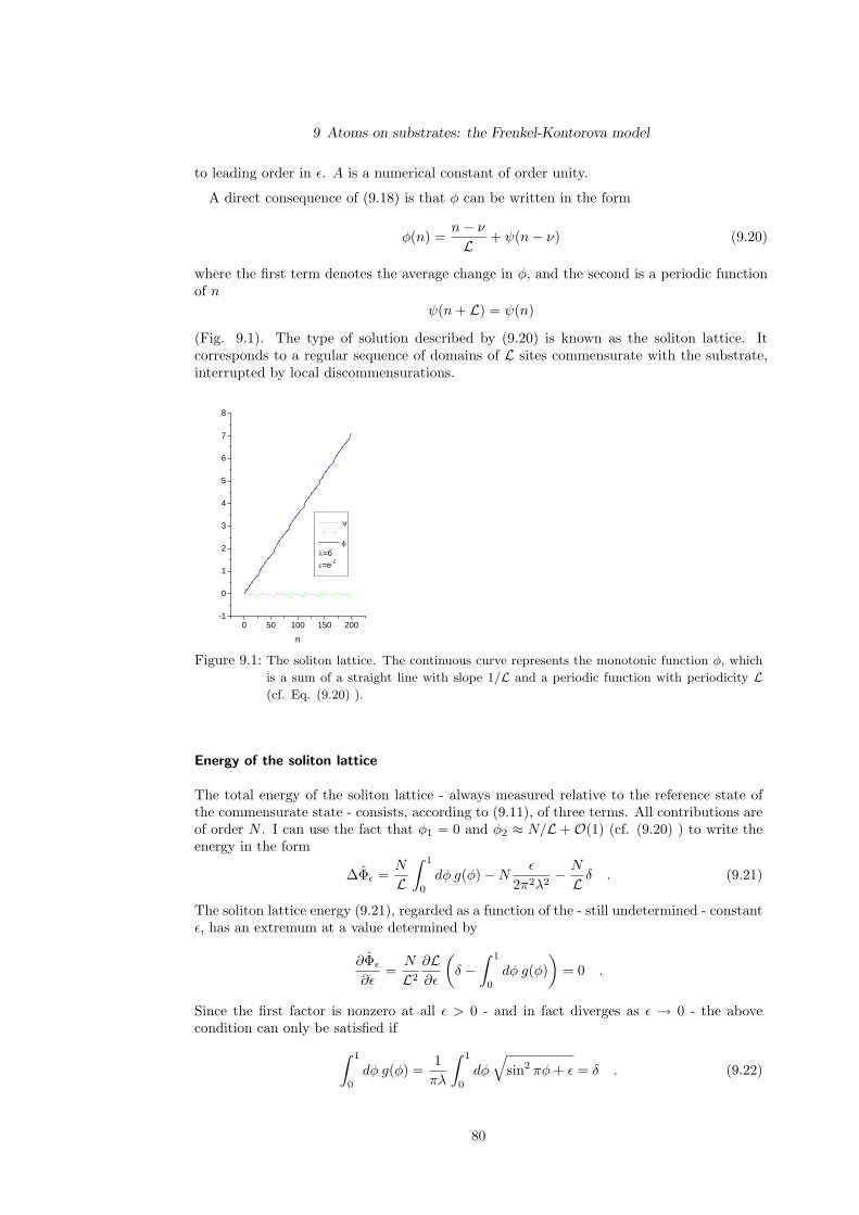
9 Atoms on substrates: the Frenkel-Kontorova model
to leading order in ε. A is a numerical constant of order unity.
A direct consequence of (9.18) is that φ can be written in the form
φ(n) =n− ν
L + ψ(n− ν) (9.20)
where the first term denotes the average change in φ, and the second is a periodic functionof n
ψ(n + L) = ψ(n)
(Fig. 9.1). The type of solution described by (9.20) is known as the soliton lattice. Itcorresponds to a regular sequence of domains of L sites commensurate with the substrate,interrupted by local discommensurations.
0 50 100 150 200-1
0
1
2
3
4
5
6
7
8
n
ψ φ
λ=6ε=e-2
Figure 9.1: The soliton lattice. The continuous curve represents the monotonic function φ, which
is a sum of a straight line with slope 1/L and a periodic function with periodicity L(cf. Eq. (9.20) ).
Energy of the soliton lattice
The total energy of the soliton lattice - always measured relative to the reference state ofthe commensurate state - consists, according to (9.11), of three terms. All contributions areof order N . I can use the fact that φ1 = 0 and φ2 ≈ N/L+O(1) (cf. (9.20) ) to write theenergy in the form
∆Φε =N
L∫ 1
0
dφ g(φ)−Nε
2π2λ2− N
L δ . (9.21)
The soliton lattice energy (9.21), regarded as a function of the - still undetermined - constantε, has an extremum at a value determined by
∂Φε
∂ε=
N
L2
∂L∂ε
(δ −
∫ 1
0
dφ g(φ))
= 0 .
Since the first factor is nonzero at all ε > 0 - and in fact diverges as ε → 0 - the abovecondition can only be satisfied if
∫ 1
0
dφ g(φ) =1
πλ
∫ 1
0
dφ
√sin2 πφ + ε = δ . (9.22)
80

9 Atoms on substrates: the Frenkel-Kontorova model
The above condition can be used to determine the value of ε = ε(δ) which, for a givenmismatch, gives an extremum of the soliton lattice energy. In order to determine the natureof the extremum we must first look at the second derivative
∂2Φε
∂ε2
∣∣∣∣∣ε=ε(δ)
= − 12(πλ)2
N
L∂L∂ε
∣∣∣∣ε=ε(δ)
.
In view of (9.19), the sign of the second derivative is positive. The local minimum thusdetermined will always have a lower energy than the reference state, by an amount
∆Φε = −Nε
2π2λ2(9.23)
(noting that the first and the third terms in (9.21) cancel out).
It should however be noted that (9.22) has a solution for ε only for such δ > δc, wherethe critical value of δ is the same as that derived in the context of the energetic stabilityof the single kink. In other words, at mismatches δ < δc, the commensurate state will stillbe favored. Once this critical value is exceeded however, not only becomes the spontaneouscreation of a single kink energetically possible, but the whole structure of a soliton lattice -a new, incommensurate phase -, acquires a macroscopic energetic advantage and is formedspontaneously.
Relationship between ε and δ
In order to to derive the explicit relationship between ε and δ, I must go back to (9.22). Fornotational simplicity let me from now on drop the bar from the ε. I first note that
dδ
dε=
12π2λ2
L(ε) ;
using the general expression
δ − δc =∫ ε
0
dεdδ
dε
and the leading-order result (9.19), I obtain
δ − δc = − 12π2λ
ε lnε
Ae
or, in reduced dimensionless form,
δ − δc
δc= −1
4ε ln
ε
Ae. (9.24)
Discommensurations repel each other
Using this relationship, it is possible to express the energy of the incommensurate phase perdiscommensuration as
∆Φε
N/L =1
2π2λε ln
ε
A
= −(δ − δc) +δc
4ε
= −(δ − δc) +8
π2λe−L/λ . (9.25)
The first term in the last line is exactly the energy (9.13) of an isolated kink. The sec-ond term, which is always positive, expresses the repulsive energy of interaction betweenneighboring discommensurations.
81

9 Atoms on substrates: the Frenkel-Kontorova model
The mean interatomic spacing
The mean interatomic spacing, defined by
a = limn→∞
xn − x0
n,
can now be calculated for the incommensurate phase. It is equal to
a = b
(1 +
1L
),
which corresponds to a winding number
r =a
b∼ 1− 1
λ ln δ−δc
δc
(9.26)
to leading order. Note that, as the mismatch approaches the critical value from above, themean spacing approaches b continuously. A singularity at critical mismatch appears in thesecond order derivative of the energy with respect to the length L = Na (check this!, ex-ercise). The commensurate-incommensurate transition is a therefore a “second order”phasetransition in the language of statistical mechanics.
Free vs. fixed-end boundary conditions
I have up to now considered free-end boundary conditions. In other words: given the materialparameters (coupling constant λ and mismatch δ) we look for the energy minimum, whichin turn determines the winding number (9.26). It is of course possible to consider fixed-endboundary conditions, in which the positions of the end atoms are held fixed. More precisely,the relevant quantity for a system of N atoms is the difference φN −φ0. Holding it constantcorresponds to fixing the winding number, i.e. the density of discommensurations L/N .The parameter ε is then determined by (9.19). The energy can be directly computed from(9.21) and the end result has exactly the form of the last line in (9.25). The interpretationis also the same: the soliton lattice has an energy which consists of contributions of theindividual discommensurations and of an interaction part, arising from the mutual repulsionof neighboring discommensurations. Note however that since we are in effect fixing thesoliton lattice, the expression for the energy is valid for any value of the misfit parameter.If δ < δc this means that the extra positive energy must be supplied in order to maintainthe fixed-end boundary conditions.
Phasons
The soliton lattice has a further important property which I have not discussed up to now.Its energy, (9.25), is independent of the integration constant ν, defined in 9.10). This meansthat the whole soliton lattice configuration can be translated by an arbitrary amount withoutan energy cost. As has been discussed in Section 8.2.4 in the context of single kinks, thistranslational invariance implies the existence of a zero-frequency (Goldstone) mode in thespectrum of linearized excitations around the exact soliton lattice configuration. Let meexamine this in some detail:
Up to now we have only looked at equilibrium properties which are determined by theminima of the total potential energy (9.3). The dynamics of the FK model is governed bythe equations of motion
φn = φn+1 + φn−1 − 2φn − 12πλ2
sin 2πφn , (9.27)
82

9 Atoms on substrates: the Frenkel-Kontorova model
or, in the continuum approximation,
∂2φ
∂t2− ∂2φ
∂n2= − 1
2πλ2sin 2πφn , (9.28)
where the time is measured in units of (m/C)1/2.
Linearization of (9.28) around the static soliton lattice configuration φs(n − ν) = (n −ν)/L+ ψ(n− ν),
φ(x, t) = φs(n− ν) +∑
q
e−iωqtfq(n) , (9.29)
leads to a Schroedinger-like equation for the fq’s
−d2fq
dn2+
1λ2
cos(2πφs) fq = ω2qfq . (9.30)
The effective potential of (9.30) has the periodicity L of the soliton lattice. Consequently,the Bloch/Floquet theorem applies to the eigenfunctions:
fq(n) = eiqnFq(n) whereFq(n) = Fq(n + L) (9.31)
Now the eigenfunction corresponding to the Goldstone mode is
dφs
dn=
1L + ψ′(n− ν)
and is therefore periodic in n with period L. By comparison with (9.31) we conclude thatit must correspond to q = 0 and that F0(n) = dφs/dn.
Note the contrast with the situation encountered in the context of localized kinks; in thatcase the zero-frequency mode was a discrete state in the spectrum. Now it is part of aband. In fact, the spectrum ωq consists of (i) a low-q region, starting at zero and reachingout to π/L, with a linear dependence of ωq, and (ii) a high-q region, i.e. at wavelengthsshorter than the the distance L between discommensurations, which is dominated by theshort-range properties of the soliton lattice, which are effectively those of the commensuratephase. Region (i) gives rise to the so called phason branch of excitations, region (ii) to theoptical phonon branch of the commensurate phase. The two branches are separated by afrequency gap.
9.2 Breaking of analyticity
The treatment of the FK model up to now has been based on the continuum approximation,which will break down at values of λ ≤ 1. It is then necessary to treat the equilibria of thepotential energy in terms of the second-order recurrence equation (9.5), i.e. to go back tothe standard map of Section 7.3.5. When applying results from that section, it should benoted that the correspondence is qn → φn−1/2 and K → λ−2. The next section will mostlytreat the case of fixed end points. The implications for the physically relevant case of freeboundary conditions will be treated somewhat heuristically.
83

9 Atoms on substrates: the Frenkel-Kontorova model
9.2.1 FK ground state as minimizing periodic orbit of the standard map
Rational winding numbers
If the ends are held so that the average interatomic distance is a rational multiple of thesubstrate periodicity (in the language of the standard map this corresponds to a rationalwinding number), i.e.
φN − φ0
N= w =
r
s,
where r, s are integers, the energy minimum (ground state) will be an (r, s) orbit of thestandard map, i.e. an s−cycle such that φs+1−φ1 = r. This corresponds to a commensuratestate and holds for any value of the nonlinearity.
Irrational winding numbers
The nontrivial part is of course what happens for irrational values of the winding numberw. In this case, Aubry [23] has proved the following fundamental results:
• for K < Kc (corresponding to λ > λc = K−0.5c = 1.014491), the ground state is
quasiperiodic, of the formφn = tn − α + u(tn − α) (9.32)
where tn = wn and the hull function is periodic with period 1, u(t) = u(t + 1) andanalytic in t. The ground state of the FK chain thus corresponds to a torus trajectoryof the standard map. This result effectively generalizes (9.20). As K approaches Kc,and successive KAM tori break, the hull function becomes more and more bumpy(cf. Fig. 7.8). Aubry describes this behavior as a phase transition due to breaking ofanalyticity. Indeed,
• for K > Kc (corresponding to λ < λc = K−0.5c = 1.014491), the ground state is still
quasiperiodic, given uniquely by (9.32). However, it now corresponds to a cantorusof the standard map (cf. Fig. 7.10). Accordingly, the corresponding hull functiondevelops discontinuities (Fig. 9.2, left and center panels).
0.0 0.2 0.4
0.00
0.05
0.10
u
t
0.0 0.2 0.4 0.6 0.8 1.0
0.0
0.2
0.4
0.6
0.8
1.0
u+t
t
0 20 40 60 80 1000.0
0.5
1.0
1.5
2.0
0 2 4 6 8 100.0
0.1
0.2
0.3
0.4
0.5 ω
j
Figure 9.2: Left panel: the hull function, as represented by an 89-cycle rational approximation
of a cantorus for K = Kc + 0.3. Center panel: the function u(t) + t allows -within
this finite approximation- a better view of the gaps. Right panel: the phonon spectra
corresponding to this ground state. Note that the minimal frequency is nonzero (inset).
84

9 Atoms on substrates: the Frenkel-Kontorova model
9.2.2 Small amplitude motion
Small amplitude motion around the ground state is described by linearizing the equationsof motion (9.27) around the ground state, i.e.
φn(t) = φGSn +
∑q
f (j)n e−iωjt
which leads to the eigenvalue equation∑
n
hmnf (j)n = ω2
j f (j)m (9.33)
where
hmn =∂2Φ
∂φn∂φm(9.34)
and the second derivatives are evaluated at the ground state positions defined by (9.32).The eigenvalues of the Hessian matrix correspond to the squares of the eigenfrequencies oflocal oscillations (phonon spectra).
We have seen in section 7.3.1 and in the beginning of the present chapter that all tra-jectories of the standard map correspond to local extrema of the potential energy functionΦ. Local extrema can be classified according to the properties of the eigenvalues of (9.33).If a single eigenvalue is negative, the extremum is unstable (maximum in at least one di-rection). If all eigenvalues are positive it is a local minimum, i.e. in general a metastableconfiguration. A zero eigenvalue (Goldstone mode) indicates an invariance of the energywith respect to a particular motion. We saw an example of this in the case of the solitonlattice - which was a stable configuration (a ground state of the FK chain) in the continuumapproximation. In fact the spectra of torus-like ground states obtained below the thresholdof analyticity breaking always include such a zero-frequency mode, indicating that the totalenergy is invariant with respect to a change of phase; the whole arrangement can slide freely.Above that threshold, the atomic arrangement of adatoms becomes “pinned” . Pinning isreflected in the phonon spectrum which develops a gap near zero frequency (cf. Fig. 9.2,right panel). Peyrard and Aubry [24] performed extensive numerical studies of the transitionby breaking of analyticity and demonstrated that the gap frequency vanishes as the thresh-old is approached. More specifically, they determined that the minimal frequency scales asa power of K −Kc,
ωmin ∝ (K −Kc]χ
where 1 < χ < 1.03.
9.2.3 Free end boundary conditions
The picture which emerges for the physically relevant case of free-end boundary conditionsis the following: The average interparticle distance a as a function of the misfit parameteris characterized by locked-in, flat regions, at rational winding numbers, which correspond tocommensurate phases. As long as the nonlinearity is below threshold, these flat regions areinterrupted by intervals of continuous variation of a with δ, which correspond to irrationalwinding numbers (incommensurate phases); the function a(δ) forms an incomplete devil’sstaircase. At the threshold of analyticity breakup, there are steps at every rational valuesof the ratio a/b, separated by discontinuities. This is the complete devil’s staircase (cf. thesimilar analysis of phase locking in the case of the circle map in section 7.3.8). Numericalresults [25] are summarized in Fig. 9.3.
85

9 Atoms on substrates: the Frenkel-Kontorova model
Figure 9.3: Left panel: Phase diagram (winding number vs. misfit parameter) for the FK model.
The numbers represent values of the locked-in winding number. Unlabeled regions
contain additional structure. Right panel: winding number as a function of misfit
parameter for the FK model at K = 1, showing a devil’s staircase structure (from
[25]).
9.3 Metastable states: spatial chaos as a model of glassystructure
Chaotic trajectories of the standard map - which proliferate beyond the threshold of ana-lyticity breakup - have a special significance in the context of the FK model. A lot of themcorrespond to unstable extrema. On the other hand, a great number of them (of order eN )represent local minima, i.e. metastable states. The number and the energy distribution of
Figure 9.4: Left panel: The number of metastable equilibrium states vs. their energy per site
(measured from the ground state energy). Bands are shown for K = 5 (6 upper
segments) and K = 2 (5 lower segments); horizontal dashed lines show the border
between energy bands. Right panel: Band energy spectrum of the same equilibria vs.
K (upper scale) and the phonon gap (lower scale); bands are marked by filled areas
corresponding to a given K value (from [26]).
these metastable states have been recently computed [26]. They were found to bundle inenergy bands. The left panel of Fig. 9.4 shows the bands and their populations for K = 2and K = 5 and a golden mean winding number. The energies lie very close to the groundstate. For example, in the case of K = 2, the lowest energy band has an energy per site of10−13 (in dimensionless units). The right panel shows the relationship of energy bands tothe ground state. Since the ground state is a cantorus, it is characterized by a nonzero Lya-
86
9 Atoms on substrates: the Frenkel-Kontorova model
pounov exponent - which is itself proportional to the minimal frequency of small oscillationsfound in the previous section. Small perturbations in the displacements of the boundarysites - while still compatible with the fixed winding number - generate an exponentially largenumber of extra trajectories branching out of the cantorus with energies exponentially closeto that of the cantorus.
The type of energy landscape described above is characteristic of disordered condensedmatter systems, such as glasses or globular proteins. In this sense, the FK model providesconsiderable insight regarding the interplay of nonlinearity and disorder.
87
10 Solitons in magnetic chains
10.1 Introduction
Anisotropic exchange interactions between localized magnetic moments cause many mag-netic materials to assume an effectively one-dimensional character. Within a certain rangeof temperatures, interactions along chains of magnetic atoms can be far more significantthan interactions across chains. It is then possible to describe material properties (staticsand dynamics) in terms of a one-dimensional Hamiltonian
H = −J∑
n
~Sn · ~Sn+1 + A∑
n
(Szn)2 − µ~B ·
∑n
~Sn . (10.1)
Here, ~Sn is the spin which resides at the n-th magnetic site, J the exchange interaction(positive for a ferromagnet, negative for an antiferromagnet), A the anisotropy (“easy-plane”- if A > 0 and “easy-axis”- if A < 0), and ~B the external magnetic field. Themagnetic moment of the n-th spin is, following the standard notation, equal to µ~Sn.
A typical example of a magnetic chain capable of supporting nonlinear excitations isCsNiF3 in the paramagnetic regime T > TNeel = 2.65K, with parameters S = 1, J/kB =23.6K, A/kB = 4.5K, µ = gµB with a gyromagnetic ratio g = 2.28 (µB = is the Bohrmagneton) [27].
For some applications it is possible to neglect the explicit quantum nature of the spinoperators. In this case, ~Sn will be treated as a classical spin vector of length S (rather thanthe technically correct [S(S + 1)]1/2.
10.2 Classical spin dynamics
10.2.1 Spin Poisson brackets
Spin is an intrinsically quantum phenomenon. The way to deal with it at a classical level isby associating an appropriate Poisson bracket algebra directly with spin angular momentumvectors ~In
f, g = εαβγ∂f
∂Iαn
∂g
∂Iβn
Iγn (10.2)
where εαβγ is the antisymmetric Levi-Civita tensor (=1 if αβγ is a cyclic permutation, -1 if anticyclic, and zero otherwise) and the Einstein summation convention over repeatedsymbols is implied. A special case of (10.2) is
Iαm, Iβ
n = εαβγδmnIγn (10.3)
where δmn = 1 if m = n and 0 otherwise.
The Poisson bracket algebra defined above can be used to generate Hamiltonian dynamics
Iαn = Iα
n ,H = −εαβγIβn
∂H
∂Iγn
, (10.4)
88

10 Solitons in magnetic chains
or, in vector form,~In = −~In × ∂H
∂~In
.
I will mostly deal with dimensionless spin vectors defined as ~Sn = ~In/h; for these, theequations of motion take the form
~Sn = − 1h
~Sn × ∂H
∂~Sn
. (10.5)
Note that the Poisson brackets (10.3) can be obtained from the standard spin commutationrelations by using the correspondence principle. Note further that, independently of thedetails of the spin Hamiltonian, according to (10.5), the norms of all vectors |~Sn| remainconstant in time.
Introducing the one-dimensional Hamiltonian (10.1) into (10.5) results in
~Sn =J
h~Sn × (~Sn+1 + ~Sn−1)− 2
A
h(~Sn · z)~Sn × z − γ ~B × ~Sn (10.6)
where µ = hγ and z is a unit vector in the z-direction.
We will deal with various special cases of (10.6), which governs the nonlinear dynamics ofa broad class of one-dimensional spin chains.
10.2.2 An alternative representation
The polar form of the spin angular momentum vector ~In of length I
Ixn = I sin θn cosφn
Iyn = I sin θn sinφn
Izn = I cos θn (10.7)
can be used to provide an alternative representation of spin dynamics. The transformation
Pn = Izn = I cos θn
qn = arctan(
Iyn
Ixn
)= φn (10.8)
can be shown to be canonical, i.e. it preserves Poisson brackets:
εαβγ∂f
∂Iαn
∂g
∂Iβn
Iγn =
∑n
[∂f
∂qn
∂g
∂Pn− ∂f
∂Pn
∂g
∂qn
](10.9)
holds for any pair of functions f, g. The P ’s and q’s are canonically conjugate sets ofcoordinates and momenta, in the sense that
qm, Pn = δmn (10.10)
(with any of the two expressions of Poisson brackets). The two representations are equivalent- and so are the resulting dynamics. In the polar representation the dynamics takes the usualsymplectic form
qn = qn,H =∂H
∂Pn
Pn = Pn, H = −∂H
∂qn. (10.11)
89
10 Solitons in magnetic chains
Again, I will use the dimensionless polar variable
pn = Pn/h = S cos θn ;
the equations of motion then take the form
hqn =∂H
∂pn
hpn = −∂H
∂qn. (10.12)
10.3 Solitons in ferromagnetic chains
10.3.1 The continuum approximation
If the exchange constant J in (10.1) is positive, and in the absence of anisotropy and externalfields, spins will tend to a parallel ordering. This is exactly true at zero temperature. Itdefines a ferromagnetic ground state Sz
n = S, Sxn = Sy
n = 01. At reasonably low temperatures,where thermal motion does not prevail, it is plausible to assume that spin orientations donot vary wildly from site to site. Thus, although the spin vector may be far from the“reference” state (0, 0, 1), it will still make sense to write down a continuum approximation.This approximates sites n by a continuous index variable, n → x, and individual spins by acontinuum field, ~Sn → ~S(x). Sums over n are approximated by integrals, with the rule
∑n
· · · →∫
dx
a· · ·
where a is the lattice constant. Spins at neighboring sites can be obtained by Taylor expan-sion
~Sn±1 → ~S(x± a) ≈ ~S(x)± a~S′(x) +12a2~S′′(x) + · · ·
where the primes denote derivatives with respect to x. According to the above rules,
~Sn · ~Sn+1 → |~S(x)|2 + a~S(x) · ~S′(x) +12a2~S(x) · ~S′′(x) .
The first term is the constant norm of the spin vector field. The second term is proportionalto the derivative of the constant norm, therefore vanishes. The third term can be integratedby parts over all space (the contribution from the boundary vanishes identically). Theresulting continuum version of the Hamiltonian (10.1) is
H =12Ja
∫dx
(∂~S
∂x
)2
+A
a
∫dx S2
z −µ
a~B ·
∫dx ~S . (10.13)
The spin equations of motion (10.6) reduce, in the continuum limit, to
~S =Ja2
h~S × ~S′′ − 2A
h
(~S · z
) (~S × z
)− γ ~B × ~S . (10.14)
Comment: (10.14) may also be obtained by taking the continuum limit of (10.4). Thecorrespondence is
∂
∂~Sn
→ aδ
δ~S(x)1Note that the choice of the z direction is at this stage - with the full rotational invariance of the exchange
interaction - entirely arbitrary.
90
10 Solitons in magnetic chains
where the right-hand side corresponds to a functional derivative. (10.4) becomes
~S(x) = −a
h~S(x)× δH
δ~S(x)
which, if we insert the functional derivative
δH
δ~S(x)= −Ja~S′′ +
A
a
(~S · z
)z − µ
a~B ,
reproduces (10.14).
In what follows, I will also need the continuum limit of the alternative (polar) spin repre-sentation.
p(x) = Sz(x), , q(x) = arctanSy
Sx
The Hamiltonian (10.13) can be transformed directly to the polar variables if we note that
S′x2 + S′y
2 =(pp′)2
S2 − p2+ (S2 − p2)q′2 .
The result is
H =12Ja
∫dx
S2
S2 − p2p′2 + (S2 − p2) q′2
+A
a
∫dx p2 − µ
aB
∫dx
√S2 − p2 cos q , (10.15)
where I have chosen to take the x-axis of the spin vector parallel to the magnetic field.
10.3.2 The classical, isotropic, ferromagnetic chain
The isotropic ferromagnetic chain is described by the Hamiltonian (10.1) with A = 0. Iwill choose the z direction along the magnetic field. The classical spin dynamics in thecontinuum limit are described by (10.14). In polar canonical variables these transform to
p =Ja2
h
[(S2 − p2)q′
]′
q = −Ja2
h
[S2p′′
S2 − p2+
S2p p′2
(S2 − p2)2+ p q′2
]− µB
h.
In the following I will use dimensionless units, i.e. measure lengths in units of the latticeconstant and times in units of h/(JS). The magnetic field will be denoted by the dimension-less quantity b = µB/(JS). Finally, I set p → Sp. The equations of motion in dimensionlessform are
p =[(1− p2)q′
]′
q = − p′′
1− p2− p p′2
(1− p2)2− p q′2 − b . (10.16)
91

10 Solitons in magnetic chains
Soliton solutions
I look for bounded propagating solutions of the type
p = p(x− vt)q = Ωt + q(x− vt) (10.17)
where the extra term allows for an overall precession around the z axis. In addition toboundedness, the solution should decay at infinity, and approach the ferromagnetic groundstate p → 1
The equations of motion transform to the following system of coupled ODEs:
−vp′ = (1− p2)q′′ − 2pp′q′ =[(1− p2)q′
]′
Ω− vq′ = − p′′
1− p2− p p′2
(1− p2)2− p (q′)2 − b (10.18)
We note that the upper equation has a first integral, which we write as
q′ = −v(p− p0)1− p2
(10.19)
- where p0 is a constant to be chosen later - and use to eliminate q from the lower equation.After rearranging some terms I obtain
p′′
1− p2+
p p′2
(1− p2)2= −v2 (p− p0)(1− p0p)
(1− p2)2− Ω
where Ω = Ω + b. Multiplying this by 2p′ produces a complete derivative on the left-handside:
(p′2
1− p2
)′= −2v2 (p− p0)(1− p0p)p′
(1− p2)2− 2Ωp′
= −2v2
[p20 − 2p0p + 12(1− p2)
]′− 2Ωp′
which can be integrated to give
p′2
1− p2= −v2 p2
0 − 2p0p + 12(1− p2)
− 2Ωp + p1
where p1 is a new integration constant.
Now the requirement of boundedness, applied to the derivative q′ as p → 1, demands (cf.(10.19)) that p0 = 1. As a consequence,
(p′)2 = (1− p)[(1 + p)(p1 − 2Ωp)− v2
]. (10.20)
An analytically favorable choice of the integration constant p1 can be made by demandingthat the brackets vanish at p = 1. This means taking
p1 = 2Ω + v2
and results in (dp
dx
)2
= (1− p)2[2Ω(1 + p)− v2
]. (10.21)
92
10 Solitons in magnetic chains
Note that, in order for the right-hand side to be positive at least for some values of p, theconditions Ω > 0 and v2 < 4Ω must hold. I therefore set
v = 2Ω1/2 cosα
2(10.22)
and obtain2Ω1/2 dx
dp= ± 1
(1− p)(p− cosα)1/2
which can be formally integrated as
2Ω1/2(x− x0) =∫ p
cos α
dp1
(1− p)(p− cos α)1/2
=21/2
sin α2
tanh−1
[(p− cos α)1/2
21/2 sin α2
],
or, after some rearrangement,
p(x) = 1− 2 sin2 α
2sech2
Ω1/2 sin
α
2(x− vt− x0)
. (10.23)
Inserting (10.23) in (10.19) gives
q′ =v/2
1− sin2 α2 sech2
Ω1/2 sin α
2 (x− x0)
which can be integrated to give
q = q0 + Ωt +v
2(x− vt− x0) + tan−1
tan
α
2tanh[Ω1/2 sin
α
2(x− vt− x0)]
(10.24)
-where I have reverted to the original dynamical variable q.
Eqs. (10.23) and (10.24) describe a soliton with an internal degree of freedom: in additionto its overall translational motion with velocity v, the soliton is characterized by a nonuni-form internal precession of each spin with respect to the z-axis (Fig. ). The soliton solutioncontains two independent parameters, the internal precession frequency and α, which com-pletely determine the soliton dynamics. In particular, the translational velocity is given by(10.22), the soliton spatial extent is (in units of the lattice constant a)
Γ =1
Ω1/2 sin α2
and the amplitude - as defined by the maximum deviation of p from the ferromagneticallyordered state p = 1 -
A = 2 sin2 α
2.
In addition, the soliton solution contains the arbitrary constants x0, q0 which specify, re-spectively, the initial position and internal phase.
Soliton magnetization
The total magnetization carried by the soliton - measured, in units of h, with respect to theferromagnetically ordered state - is
M =∑
n
(Szn − S)
= S
∫ ∞
−∞dx (p− 1)
= −4Ssin α
2
Ω1/2. (10.25)
93

10 Solitons in magnetic chains
In what follows, it will prove useful to express the soliton’s translational velocity in termsof M , i.e.
v =4S
|M | sin α
=4JS2a
h|M | sinα , (10.26)
where in the second line I have reintroduced the physical units.
Soliton energy
I will restrict myself to the case of vanishing external field B = 0. In this case Ω = Ω. Theenergy density is, from (10.15) and (10.17),
12JS2
p′2
1− p2+ (1− p2)q′2 ,
or, using (10.21) and (10.19),JS2Ω(1− p)
which integrates to
E = 4JS2Ω1/2 sinα
2
= 16JS3 1|M | sin
2 α
2. (10.27)
where in the second line I have eliminated the precession frequency in favor of the magne-tization.
It turns out that the set of dynamical variables M and
P = 2hSα/a (10.28)
are a better choice for describing the dynamics of the soliton. This becomes clear by lookingat the derivative (
∂E
∂P
)
M
=4JS2a
h· sin α
|M | = v ,
which indicates that P can be interpreted as the canonical momentum conjugate to theposition of the soliton.
Semiclassical quantization
Systems which are classically integrable may be quantized according to the Bohr-Sommerfeldscheme, which demands that the total action along a closed orbit must be a multiple ofPlanck’s constant
J =∑
j
∮pjdqj = nh (10.29)
where pj , qj is a set of canonically conjugate coordinates and momenta.
The canonically conjugate polar spin coordinates defined in subsection 10.2.2 may be usedin the above quantization condition after an appropriate correction for their dimensions.Since polar spin coordinates are dimensionless an extra factor h must be added to the left-hand side of the action (cf. the extra factor h which appears in the equations of motion
94

10 Solitons in magnetic chains
(10.12) ). Furthermore, since in this section we have made the substitution p → Sp, thequantization condition over a motion which is periodic with period T reads
Sh∑
j
∫ T
0
dt pj qj = nh
or, going to the continuum limit (with the length measured in units of the lattice constant),∫ N/2
−N/2
dx
∫ T
0
dt (p− 1) q =2πn
S. (10.30)
Note that I have used p−1 rather than p, since I am interested in the properties of a localizedsoliton excitation, which approaches p → 1 as x → ±∞.
There are two types of periodic motion associated with the soliton:
• The first is related to the translational motion. In other words, the soliton runsaround the chain (which is in this case subjected to periodic boundary conditions)with a period T = N/v. This is best viewed in a coordinate system which rotates withangular velocity Ω around the z-axis. In this case
q = −vq′ = −v2 11 + p
and the left-hand side of (10.30) becomes
−v2
∫ N/v
0
dt
∫ N/2
−N/2
dxp− 11 + p
= v2
∫ N/v
0
dt Ω−1/2
∫ ∞
−∞dξ 2 sin
α
2· sech2ξ
2− 2 sin2 α2 sech2ξ
= v2Ω−1/2 sinα
2· N
v·∫ ∞
−∞dρ
1cosh ρ + cosα
= N Ω−1/2 2Ω1/2 cosα
2sin
α
2· 2α
sin α= 2Nα .
In terms of P , the canonical momentum of the soliton given by (10.28), the quantiza-tion condition reads
P ≡ hK = 2πn
Nah (10.31)
which is the usual quantization condition for the momentum of a free particle subjectto periodic boundary conditions.
• The second type of periodic motion is related to the precession around the symmetryaxis. In this case I consider a coordinate system moving with the soliton translationalvelocity v. Then
q = Ω
p = 1− 2 sin2 α
2· sech2
[Ω1/2 sin
α
2· x
]
and the left-hand side of (10.30) becomes
−Ω∫ 2π/Ω
0
dt
∫ N/2
−N/2
dx 2 sin2 α
2· sech2
[Ω1/2 sin
α
2· x
]
95

10 Solitons in magnetic chains
= −Ω2π
Ω2 · sin α
2· Ω−1/2 · 2
= 2πM
S(10.32)
and the quantization condition simply expresses the fact that
M = m .
In order to complete the semiclassical quantization scheme, I rewrite the relation betweenenergy and canonical momentum, or, as is more usual in condensed matter physics, thewavevector K. Equation (10.27) now reads
E = 16JS3 1|M | sin
2
(Ka
2S
). (10.33)
In the special case S = 1/2, the above expression coincides with the exact quantum me-chanical result found by Bethe, using the Bethe-Ansatz, for bound states of M magnons2.
10.3.3 The easy-plane ferromagnetic chain in an external field
Weak out-of-plane motion: the Sine-Gordon limit
I will consider the case of strong anisotropy. The spin vectors are then approximatelyconfined to the xy plane. The z component is small, so we can readily assume p ¿ S andset p′ ∼ 0 in (10.15). The continuum Hamiltonian becomes
H =12JaS2
∫dx q′2 +
A
a
∫dx p2 − µ
aBS
∫dx cos q . (10.34)
Inserting the relevant functional derivatives
δH
δp(x)= 2
A
ap
δH
δq(x)= −JaS2q′′ +
µBS
asin q (10.35)
into the equations of motion, I obtain
q =a
h
δH
δp(x)=
2A
hp
p = −a
h
δH
δq(x)=
Ja2S2
h− µBS
hsin q (10.36)
from which I can eliminate p and get a differential equation which is of second order in spaceand time for q:
∂2q
∂t2− c2 ∂2q
∂x2= −ω2
0 sin q (10.37)
wherec =
√2AJ
aS
h
and
ω0 =√
2AµBS
h.
2From a more modern perspective, bound states of magnons should be appropriately called quantumsolitons
96

10 Solitons in magnetic chains
We recognize (10.37) as the SG equation. We have derived it under the assumption of stronganisotropy. Moreover, in order for (10.37) to provide a meaningful approximation to the truedynamics of discrete spins, the length scale defined by (10.37)
d =c0
ω0=
(J
µBS
)1/2
a
should be considerably larger that the lattice constant. The inequality
B ¿ J
µS
therefore defines the physical range of allowed magnetic fields consistent with contiuum SGdynamics.
Making use of the first of the equations of motion (10.36) I can write the total energy asa function of the field q only:
H = ε0
∫dx
12
(∂q
∂t
)2
+12
c20
(∂q
∂x
)2
+ ω20 cos q
. (10.38)
where ε0 = JaS2/c20. This allows me to effectively ignore the out-of-plane motion and deal
with q as if it were a single scalar field with an effective Lagrangian density
L = ε0
12
(∂q
∂t
)2
− 12
c20
(∂q
∂x
)2
− ω20 cos q
- which results in the SG dynamics and the total energy (10.38). Note however that thisshould not be misunderstood to imply a vanishing out-of-plane motion.
Dynamical structure factor
The quantity
Iαα(k, t) =1N
∑m,n
eik(m−n)a < Smα (t)Sn
α(0) > ,
where the brackets denote a thermodynamic average over a canonical ensemble, measuresthe spatial Fourier transform of time-dependent correlations of the α-component of spins.Its temporal Fourier transform is the dynamical structure factor (DSF)
Iαα(k, ω) =∫ ∞
−∞
dt
2πe−iωtIαα(k, t)
=1a
∫dt
2π
∫dx ei(kx−ωt) < Sα(x, t)Sα(0, 0) > , (10.39)
where in the second line I have made use of the system’s translational invariance and, inaddition, taken the continuum limit. The DSF can be experimentally deduced from inelasticneutron scattering experiments which detect k and hω, as the change in the neutron’smomentum and energy, respectively.
In the case of weak out-of-plane motion, the xx DSF can be written in terms of the q-fieldas
Ixx(k, ω) =S2
a
∫dt
2π
∫dx ei(kx−ωt) < cos q(x, t) cos q(0, 0) > .
97

10 Solitons in magnetic chains
DSF calculation for a dilute gas of solitons
In the limit of weak out-of-plane motion, spin dynamics is effectively governed by the SGequation. Now the dynamics of the SG field equation, a completely integrable system,is truly exceptional. For decaying boundary conditions it implies that solitons have anessentially infinite lifetime. At a finite temperature (therefore finite energy density) theexact mathematics is somewhat more subtle, but there are good reasons to believe in theexistence of a soliton gas. At low temperatures, such a kink (or antikink)-like soliton gaswould consist of almost non-interacting particles of mass
M =8dε0 = 8J
(S
c0
)2a
d,
velocity-dependent energy
E(v) = Mc20γ ≡ Mc2
0
(1− v2
c20
)−1/2
≈ Mc20 +
12Mv2 + · · ·
(with the second expression valid at low velocities) and displacement field (cf. )
cos q(x, t) = 1− 2 sech2
γ(x− vt− x0)
d
where x0 is a constant specifying the soliton position at time t = 0. The last equation impliesthat, far from the soliton position, spins are oriented along the ferromagnetic reference state.Only within a distance d from the soliton do spins deviate appreciably from that referencestate. Now if the soliton gas is dilute, i.e. the density is much smaller than a/d, then it isvery improbable that two solitons will be at the same place at the same time. We can thenassume that
cos q(x, t) ≈ 1− 2∑
j
sech2
γj(x− vjt− x0
j )d
where the sum runs over all solitons of the gas.
The correlation function
< cos q(x, t) cos q(0, 0) > = 1− 2∑
j
< sech2
γj(x− vjt− x0
j )d
>
− 2∑
j
< sech2
γjx
0j
d
> (10.40)
+ 4∑
i,j
< sech2
γj(x− vjt− x0
j )d
sech2
γjx
0i
d
>
consists of four terms. The first three are constant in time and space and therefore generatecontributions to the DSF only at zero momentum and energy transfer. The same holds forthat part of the fourth term which comes from terms i 6= j and can be factorized into space-and time-independent averages. The only contribution to the DSF at nonzero k and ω willcome from the i = j part of last term (incoherent scattering) and - after averaging - is thesame for all solitons. The sum over j generates a factor equal to the total number of solitonsNs.
The averaging operation involves averaging over all initial positions and velocities of thejth soliton. The initial positions are uniformly distributed (remember that there is no
98
10 Solitons in magnetic chains
energy cost involved in moving a SG kink from one position to another). The velocities aredistributed according to the Boltzmann distribution appropriate for a one-dimensional gas.In the limit of low temperatures, relativistic corrections can be neglected and
P (v) = Ce−βMv2
2 , (10.41)
where β = 1/(kBT ) and C = (βM/2π)1/2. Symbolically, the averaging operation can bedenoted as
< · · · >=1L
∫dx0 dv P (v) · · · .
The resulting DSF
Ns
L
∫dt
2πdx0 dv dx e−i(kx−ωt)P (v) < sech2
γj(x− vt− x0)
d
sech2
γjx
0
d
>
is a quadruple integral. Setting ξ = x − vt − x0 allows the integration over x0 and ξ to bereadily performed, resulting in
ns
∫dt
2πdv ei(kvt−ωt) P (v)
[f
(kd
γ
)]2
wheref(κ) =
∫ ∞
−∞dx e−iκxsech2x
is the soliton form factor and ns = Ns/L the density of solitons. The time integral generatesa delta function of v−ω/k which then enables us to perform the integration over velocities.The resulting DSF is
I(k, ω) = ns1k
[f
(kd
γ
)]2
P (ω
k)
where γ = (1 − (ω/c0k)2)−1/2. At low temperatures kBT ¿ Mc20, where the velocity
distribution is well approximated by (10.41), this is well approximated by the Gaussiancentral peak (CP)
I(k, ω) = nsπ−1/2
Γk[f(kd)]2 e−ω2/Γ2
k
with a width
Γk =(
2kBT
M
)1/2
k .
The observed CP width in CsNiF3 is consistent with the above predictions [27].
10.4 Solitons in antiferromagnets
10.4.1 Continuum dynamics
The starting point is the spin Hamiltonian (10.1) and the resulting equations of motion(10.6) with J < 0.
In the following, I will use A = 2δ|J |; the dimensionless measure of the anisotropy will beassumed to be small. Consider first the case A = 0, B = 0. If zero-point classical fluctuationsare neglected, the ground state of the isotropic antiferromagnet at zero external field is theNeel state,
~Sn = ±(−1)nSn
99
10 Solitons in magnetic chains
where besides the rotational degeneracy (arbitrary direction of the unit vector n), there isan “even-odd” degeneracy. If A denotes “up” and B denotes “down”, both ABABAB · · ·and BABABA · · · are possible ground states with the same energy. The existence of twodegenerate “vacua” makes antiferromagnets a priori good candidates as soliton bearing sys-tems.
I will define new vector fields which are well suited to describe the situation at low temper-atures, i.e. not too far from the ground state. Note that this will not exclude large amplitudefluctuations; however, I will make the demand that the various field configurations shouldvary smoothly in space. Let
~φn =1
2S(~S2n+1 − ~S2n)
~ln =12(~S2n+1 + ~S2n) . (10.42)
The new fields satisfy the properties
~φn ·~ln = 0 (10.43)
and
|~φn|2 +1S2|~ln|2 = 1 . (10.44)
If field configurations vary smoothly in space, it is possible to use a continuum field approx-imation ~φn → ~φ(x) with field values at neighboring sites (note that a neighboring site of thenew field is at a distance 2a apart!)
~φn±1 ∼ ~φ(x)± 2a~φ ′(x) +12(2a)2~φ ′′(x) ,
and a similar expansion for ~l(x). Note however that the two fields do not have the samestatus. At the Neel state, it is obvious that |~l| = 0, whereas |~φn| = 1. In fact, a consistentfield expansion treats ~l as a small quantity, of the order of ~φ′. Therefore, terms of secondorder in ~l will be dropped. Under these conditions, the normalization condition (10.44) isexhausted by the ~φ field, which will henceforth be treated as a vector of unit length.
It is a tedious but straightforward - and necessary - exercise to use the inverse relations
~S2n = ~ln − S~φn
~S2n+1 = ~ln + S~φn (10.45)
and express the total Hamiltonian in the form
H =∫
dxH
where the Hamiltonian density is given in terms of the new vector fields:
H =1
2gc
c2
∣∣∣∣~φ ′ −2
aS~l
∣∣∣∣2
+ c2∣∣∣~φ ′
∣∣∣2
− 2ω21δ
∣∣∣~φ⊥∣∣∣2
− 4γω1
S~B ·~l
(10.46)
The first two terms come from the isotropic exchange term; the third term comes from theanisotropy - note that ~φ⊥ = ~φ−(~φ · z)z is the transverse component of the ~φ-field; the fourthterm comes from the interaction with the magnetic field. The new constants are related tothe old as follows: g = 2/(hS), ω1 = 2|J |S/h, c = ω1a.
100

10 Solitons in magnetic chains
The total magnetization can be expressed (in units of h) as3
~M =∑
n
~Sn
=∫
dx
2a2~l(x) . (10.47)
The next step is to obtain the dynamics of the coupled vector fields by differentiating bothsides of (10.42), using the dynamics defined in (10.6), and rewriting the results in terms ofthe new fields:
~φ = c~φ×(
~φ ′ − 2aS
~l
)− γ ~B × ~φ (10.48)
~l = c(~l × ~φ
)′+ caS ~φ× ~φ ′′ − ω1δS(~φ · z)~φ× z − γ ~B ×~l (10.49)
In deriving (10.48), I have further dropped anisotropy terms which are first order in ~l, if theanisotropy is small, they are negligible compared to the leading, first term in the right-handside of (10.48).
The above coupled first-order equations determine in principle the spin dynamics of thenew variables4. It is however possible to perform a further reduction by recognizing that~l is completely determined by ~φ and its derivatives (i.e. it is a slave variable). This canbe easily seen by forming the vector product of both sides of (10.48) with ~φ. After somerearrangements,
2c
aS~l = ~φ× ~φ + c~φ ′ + γ
[~B − ( ~B · ~φ)~φ
], (10.50)
which can be used to eliminate ~l from (10.49). The result is
~φ×[~φ− c2~φ ′′ + 2ω2
1δ(~φ · z)z + 2γ ~B × ~φ + γ2 ~B( ~B · ~φ)]
= 0 . (10.51)
In what follows, it will be useful to exploit (10.50) in order to eliminate the slave variable ~lfrom (10.46). The result is5
H =1
2gc
|~φ|2 − c2|~φ ′|2 − 2ω2
1δ |φ⊥|2 + γ2( ~B · ~φ)2
(10.52)
I will now consider some special cases.
10.4.2 The isotropic antiferromagnetic chain
If δ = 0 and B = 0, (10.51) is equivalent to the dynamics of the field theory defined by theLagrangian density
L0 =1
2gc
(|~φ|2 − c2|~φ ′|2
)(10.53)
subject to the constraint |~φ|2 = 1. This is the relativistically invariant nonlinear sigmamodel, which has been employed as a toy model in quantum chromodynamics. Furthermore,3Note that, strictly speaking, this holds for an even number of spins. An odd number of spins will generate
a contribution from the boundary.4It should be noted that the equations preserve exactly both the normalization |~φ|2 = 1 and the orthogo-
nality property ~φ ·~l = 0.5Strictly speaking, the result in the brackets of (10.52) omits an irrelevant constant −γ2 ~B · ~B and a total
derivative term −2γ2 ~B · ~φ′, which only generates contributions from the boundaries.
101

10 Solitons in magnetic chains
a Wick rotation shows it to correspond to the Hamiltonian of the two-dimensional classicalantiferromagnet.
The Hamiltonian density obtained from the field theory (10.53)
H =1
2gc
(|~φ|2 + c2|~φ ′|2
)(10.54)
is the same as the sum of the first two terms in (10.52).
Note: it possible to add to the Lagrangian density (10.53) a term
L∗ =1g
θ
2πS~φ ·
(~φ× ~φ ′
). (10.55)
This so called topological term of the Lagrangian does not influence the classical equationsof motion. This is because it generates a contribution to the action which depends only ongeneral topological properties of the field; in the simplest of cases, one can see, using a polarrepresentation p = φz, q = arctan(φy/φx) that
Q =14π
∫dtdx ~φ ·
(~φ× ~φ ′
)
=14π
∫dtdx
(∂p
∂t
∂q
∂x− ∂q
∂t
∂p
∂x
)
=14π
∫dtdx
∂(p, q)∂(x, t)
=14π
∫ 1
−1
dp
∫ 2π
0
dq
= 1 ; (10.56)
in general, the Pontryagin index Q of the vector field tells us how many times the vectorsweeps the unit sphere as dxdt sweeps two-dimensional space-time. The resulting contribu-tion to the action
W ∗ =∫
dx dt L∗ ,
a constant, cannot modify the classical equations of motion, which are determined by theaction derived from the Lagrangian density L0. It may however be relevant for quantumphenomena. Noting in this context that 2/gS = h and θ = 2πS 6 we obtain
W ∗
h= 2πSQ (10.57)
which hints that whether or not the extra term is relevant for quantum mechanics may welldepend on whether S is a half-integer or an integer, respectively.
10.4.3 Easy axis anisotropy
Consider the case of easy axis anisotropy δ = − 12 (ω0/ω1)
2.
The dynamics of the vector field ~φ (10.51) is equivalent to the Lagrangian field theory
L =1
2gc
(|~φ|2 − c2|~φ ′|2 − ω2
0 |~φ⊥|2)
(10.58)
6The choice θ = 2πS is mandated by the requirement that the canonical momentum conjugate to ~φ,
~π = ∂(L0 + L∗)/∂~φ should form a “triad” with ~l and ~φ, i.e π = h/a~l × ~φ and h/a~l = ~φ × ~π; the choiceθ = 2πS in (10.48) with B = 0 satisfies the first of these requirements; the second, which is a natural
feature of a Hamiltonian theory, guaranteeing the right form for ~l, the generator of infinitesimal rotations,is then automatically satisfied.
102
10 Solitons in magnetic chains
subject to the constraint |~φ|2 = 1. Note that the anisotropy term does not destroy Lorentzinvariance. The simplest way to lift the constraint is to introduce polar coordinates
α = arccos φz
β = arctan(φy/φx)
where 0 ≤ α ≤ π and 0 ≤ φ < 2π. The Lagrangian density (10.58) can then be written as
L =1
2gc
[α2 + sin2 α β2 − c2
(α′2 + sin2 α β′2
)− ω2
0 sin2 α]
. (10.59)
The corresponding energy density is given by (10.52) as
H =1
2gc
[α2 + sin2 α β2 + c2
(α′2 + sin2 α β′2
)+ ω2
0 sin2 α]
. (10.60)
The resulting equations of motion are
α′′ − 1c2
α =12
ω20 − β2
c2sin 2α
1c2
∂
∂t
(sin2 α β
)=
∂
∂x
(sin2 α β′
). (10.61)
The vacua
I first determine the spatially and temporally uniform solutions. These are α = 0, π/2, π andβ = β0 (arbitrary). By inspection of (10.60) it can be seen that only α = 0, π correspond to- degenerate - energy minima (vacua), whereas α = π/2 corresponds to an energy maximum.
Kinks and antikinks
I next look for solutions which satisfy β = ω (uniform precession of the φ vector around thez-axis) and α = 0; the latter restriction can later be lifted because I can always Lorentz-boosta static solution. The second equation is satisfied identically; the first reduces to
α′′ =ω2
0 − ω2
2c2sin 2α , (10.62)
which is a Sine-Gordon equation for the field 2α and a length scale R = c/√
ω20 − ω2. It has
a first integral
R2(α′)2 = −12
cos 2α + const
and can therefore support soliton solutions which interpolate from one vacuum (α = 0 tothe other (α = π). This implies the choice of the constant equal to 1/2, therefore
Rα′ = ± sin α
andα = 2arctan e±(x−x0)/R ,
or,
sinα = sechx− x0
R
cosα = ∓ tanhx− x0
R, (10.63)
where x0 is an arbitrary constant.
The solitons are π-kinks, going from α = 0 at x → −∞ to π at x → ∞ (and thecorresponding antikinks).
103
10 Solitons in magnetic chains
The total magnetization of the π-kink
Introducing (10.50) into (10.47), we obtain the following general expression for the magne-tization, valid for ~B = 0:
~M =S
2c
∫dx
(~φ× ~φ + c~φ′
)
The z-component of the magnetization will then be
Mz =S
2c
∫dx
[(φxφy − φyφx
)+ cφ′z
]
= − S
2c
∫dx sin2 α β +
S
2cos α|∞−∞
= m∓ S (10.64)
where the limits of integration have been extended to infinity, since we assume that the spinconfigurations approach one of the two Neel states at infinity. The second term will thenbe equal to -S for a kink and S for an antikink. This is a contribution which is entirelyindependent of the structural details of the kink. The “extra” magnetization will be
m = − S
2cω
∫ ∞
−∞dx sech2 x− x0
R
= − S
2cω · 2R
= − ω√ω2
0 − ω2S . (10.65)
The total energy of the π-kink
Introducing the form of the kink solution into the expression for the energy density (10.60)gives
H =1
2gc
[sin2 α ω2 + c2 sin2 α
R2+ ω2
0 sin2 α
]
=ω2
0
gcsech2 x− x0
R
which gives a total kink energy
E =∫ ∞
−∞dxH
=ω2
0
gc2R
=2g
ω20√
ω20 − ω2
. (10.66)
It is possible to express ω in terms of the kink magnetization m using (10.65). This givesthe energy of the kink as a function of magnetization
E = hω0
√S2 + m2 (10.67)
where I have made use of g = 2/(hS). The last form, along with (10.65), is eminentlyuseful for developing a semiclassical quantization approach where m would take integer orhalf-integer values.
104

10 Solitons in magnetic chains
10.4.4 Easy plane anisotropy
A positive value of the anisotropy parameter δ favors spin orientations along the xy-plane.Setting
δ =12
(ω0
ω1
)2
implies a change of sign ω20 → −ω2
0 in the effective Lagrangian density (10.59), which nowreads
L =1
2gc
[α2 + sin2 α β2 − c2
(α′2 + sin2 α β′2
)+ ω2
0 sin2 α]
, (10.68)
the energy density (10.60), and the equations of motion (10.61).
Although the spatially and temporally uniform solutions are the same as in the case ofthe easy-axis anisotropy, their role is reversed. There is only one stable energy minimum atα = π/2 and maxima at α = 0, π. Looking for solutions with α = 0 and β = ω leads to
α′′ = −12
1R2
sin 2α
where now
R2 =c2
ω2 + ω20
.
This is a SG equation for the field 2(π/2− α). We can write down the solution by makingthe substitution α → π/2− α in (10.63):
cosα = sechx− x0
R
sinα = ∓ tanhx− x0
R, (10.69)
where x0 is again an arbitrary constant.
Note that this type of solution does not interpolate between degenerate vacua. It drivesthe system out of the only available vacuum at x ¿ x0, leads it to the energy maximum atx = x0 and returns it to the vacuum as x À x0. The associated energy density is
H =1
2gc
[sin2 α ω2 +
(c2
R2+ ω2
0
)cos2 α
]
and will therefore lead, from the first term, to a total energy proportional to the size of thesystem, as long as ω 6= 0. If we restrict ourselves to finite-energy solutions ω must vanish,i.e. β = β0. The characteristic length becomes R = c/ω0 and the energy density
H =1
2gc2ω2
0 sech2[ω0
c(x− x0)
],
which integrates to a total kink energy
E =2g
ω0 = hω0S (10.70)
Inspection of (10.64) shows that both the bulk and the boundary contributions to themagnetization vanish.
105

10 Solitons in magnetic chains
10.4.5 Easy plane anisotropy and symmetry-breaking field
In the case of easy-plane anisotropy
δ =12
(ω0
ω1
)2
and nonzero magnetic field, it is possible to satisfy the equations of motion (vanishingbrackets in (10.51) ) by constructing a field theory based on the effective Lagrangian density
L =1
2gc
|~φ|2 − c2|~φ ′|2 − ω2
0 |~φ⊥|2
+ LB , where
LB =1
2gc
−γ2( ~B · ~φ)2 + 2γ ~B · (~φ× ~φ)
. (10.71)
Two comments are in order here concerning the second term in the second line. First,this is the most general scalar that can be constructed from the magnetic field and thefield vector ~φ and its derivatives, consistent with the property of time reversal invariance~B → − ~B, ~φ → −~φ. Second, that although the term is crucial for the dynamics -it generatesthe fourth term in the brackets in (10.51)-, it does not contribute to the energy, which isquadratic in the magnetic field (cf. (10.52) ).
I will consider the case in which the magnetic field is in the x-direction, i.e. it serves tobreak the easy-plane symmetry.
It is straightforward to derive the complete spin dynamics in polar coordinates. Theycorrespond to those of the previous subsection, with additional terms which come from thefield dependent part of the Lagrangian
LB =1
2gc
−γ2B2 sin2 α cos2 β − 2γB sinβ α− γB sin 2α cosβ β
.
The equations of motion in polar coordinates are:
α− c2α′′ − 12
sin 2α(β2 + ω20) = 2γB cos β sin2 α β − 1
2γ2B2 sin 2α cos2 β
∂
∂t(sin2 αβ)− c2 ∂
∂x(sin2 αβ′) = −γB cosβ α +
12γ2B2 sin2 α sin 2β (10.72)
I will also need the total energy density (10.52), which in polar coordinates reads
H = Hexch +Hanis +HB , where
Hexch =1
2gc
[α2 + sin2 α β2 + c2
(α′2 + sin2 α β′2
)]
Hanis = − ω20
2gcsin2 α
HB =(γB)2
2gcsin2 α cos2 β . (10.73)
The vacua
Spatially and temporally uniform solutions of (10.72) must satisfy the conditions
sin 2α[ω2
0 − γ2B2]
= 0
sin2 α sin 2β = 0 . (10.74)
106

10 Solitons in magnetic chains
If we look at the total energy of such a uniform state as a function of the field,
E = −L1
2gcsin2 α
(ω2
0 − γ2B2 cos2 β)
we see that the energy minimum, which is at α = π/2 at zero magnetic field, shifts toα = 0, π if the field exceeds the critical value Bc = ω0/γ. At moderate fields B < Bc, theminimal energy configuration will be at α = π/2, β = ±π/2.
The kinks
If the anisotropy is nonvanishing, we can assume that the out-of-plane motion will be weak.As long as α ∼ π/2, the second equation of motion will reduce to
∂2β
∂t2− c2 ∂2β
∂x2=
12γ2B2 sin 2β (10.75)
which is a Sine-Gordon equation for the angle π − 2β. It admits static (and Lorentz-boostable) kink and antikink solutions of the form
π − 2β = arctan e±(x−x0)/d
where d = c/(γB). Alternatively, we can write
cos β = sech(
x− x0
d
)
sin β = ± tanh(
x− x0
d
). (10.76)
which gives an energy density
12gc
(c2β′2 − ω2
0 + γ2B2 cos2 β)
and a total kink rest energy (measured from the vauum)
E0 = 2c
gd= hSγB = µSB .
Out-of-plane corrections
Corrections which arise from the weak out-of-plane motion may be estimated by consideringthe first of the equations of motion (10.72) which for α ∼ π/2 (so that the second space andtime derivatives can be neglected) gives
cos α(β2 + ω2
0 − γ2B2 cos2 β)
= 2γB cosβ β
For a static kink configuration, the first term on the left-hand-side vanishes7 and the thirdis at most (in the vicinity of the kink) of order γ2B2. At moderate fields B < Bc this leavesthe second term as the dominant one; hence
α =π
2+
2γB
ω20
cosβ β
which is the analog of the first of eqs (10.36) for the easy-plane ferromagnet and can be usedto estimate e.g. out-of.plane corrections to the kink energy.7Note that this estimate is even better for moving kinks, since the first term then partially cancels the
third.
107

10 Solitons in magnetic chains
The dynamical structure factors
The xx spectra< cos(x, t) cos(0, 0) >
give rise to a DSF similar to that of the ferromagnet with easy-plane anisotropy and magneticfield in the x-direction - except for a slightly different form factor due to the sech ratherthan sech2 function.
The yy spectra can be approximated by
< sin(x, t) sin(0, 0) >≈< σ(x, t)σ(0, 0) >
where σ = ±1. The approximation suggests that they act as “registers” of a spin flip everytime a soliton comes by. More precisely, we can approximate
σ(x, t) = σ(x, 0)(−1)N1(t) ,
where N1(t) is the number of times a soliton passes through the point x during the timeinterval (0, t), and
σ(x, 0) = σ(0, 0)(−1)N2(x) ,
where N2(x) is the number of solitons which are in the segment (0, x) at any given time.
The dynamical correlation can then be calculated, using the Poisson statistics whichcharacterize the spin flips, to be
< σ(x, t)σ(0, 0) >= e−2[N1(t) + N2(x)] .
The averages are straightforward to estimate:
• N2(x) is simply equal to 2ns|x|, where ns is the density of kink-type solitons (andns = ns the density of antisolitons).
• The average number of solitons passing through a point during a given time interval oflength t is given by nsu|t|, where u is the average thermal speed of solitons. If solitonscan be thought of as forming an ideal (Boltzmann) gas (cf. the analogous discussionof the ferromagnetic case in section 10.3.3) then u = (2kBT/M)1/2. This should ofcourse be multiplied by a factor of 2, to account for the antisolitons.
Putting everything together,
< σ(x, t)σ(0, 0) >= e−4ns|x|−4nsu|t|
and henceI(k, ω) =
π
k2 + Γ2k
π
ω2 + Γ2ω
(10.77)
whereΓk = 4ns
and
Γω = 4(
2kBT
M
)1/2
ns
According to the above, the main temperature and magnetic field dependence of both widthscomes from the soliton density which, in the appropriate temperature range, has a charac-teristic exponential dependence
ns ∝ e−E0/kBT .
Since the kink rest energy is proportional to the magnetic field, we expect the leading Band T dependence of the width to scale with B/T . This is borne out by experiments [28]on TMMC (cf. Fig. 10.1).
108

10 Solitons in magnetic chains
Figure 10.1: Energy and wavevector width of the central peak of TMMC. (from [28]).
109

11 Solitons in conducting polymers
11.1 Peierls instability
This is not an attempt to cover the general subject of electronic transport properties ofpolymers. A good place to start learning about the physical properties, the chemistry and thetechnological significance of semiconducting and metallic polymers is Alan Heeger’s Nobellecture[29]. The theoretical and experimental background on solitons in conducting polymershas also been reviewed by Heeger, Kivelson, Schrieffer and Su [30]. Here I will only try toconvey the main ideas about the Peierls instability, which turns a one-dimensional metallicchain into an insulator, and about how the resulting structures, if the proper conditions ofenergy degeneracy are met, can support solitons and polarons.
The exemplary substance for the present discussion is trans-polyacetylene, (CH)x. Theschematic structure shows that the backbone consists of carbon atom bonds which are neithersingle nor double. For large chains, where the end points are irrelevant, the picture of theelectronic structure is relatively simple: each carbon atom contributes a single pz electron tothe π- band. These electrons have a tendency to delocalize. One can express this in termsof a tight-binding model Hamiltonian
H0 = −∑ns
tn,,n+1
(c†n+1scns + c†nscn+1s
), (11.1)
where the cns’s denote creation and annihilation operators for electrons of spin s at the nthsite, and the hopping parameters tn,n+1 correspond to the π-electron transfer integrals.
11.1.1 Electrons decoupled from the lattice
In the absence of any coupling to the underlying lattice, the hopping parameters can beassumed to have a constant value, t0. The Hamiltonian H0 is then diagonal in Fourierspace, i.e.
H0 = −∑qs
εqc†qscqs , (11.2)
where
cqs =1√N
N∑n=1
eiqancns ; q =2π
a
n
N, n = −N
2+ 1, · · · , N
2− 1,
N
2, (11.3)
N is the number of sites and a the lattice constant, and
εq = 2t0 cos qa (11.4)
The resulting band structure is shown in unfolded and folded form in Fig. . The point tonote is that of the total N allowed values of q, N/2 lead to states of negative energy; sinceevery state can be doubly occupied (spin up/down), and there is a total of N π-electrons, thenegative energy states are all occupied, and the positive energy states are empty. Since thereis no gap between them, the one-dimensional tight-binding electronic system is metallic.
110

11 Solitons in conducting polymers
11.1.2 Electron-phonon coupling; dimerization
Suppose that the carbon atoms in the backbone are slightly displaced from their referencepositions. Let the displacement of the nth carbon atom be yn. It is reasonable to assumethat if the distance from the nth to the n + 1st atom decrease, the probability amplitudefor electron hopping should increase; for small relative displacements
tn,n+1 = t0 − α(yn+1 − yn) (11.5)
should hold. Furthermore, the atomic displacements contribute to a lattice deformationenergy
HL =12K
∑n
(yn+1 − yn)2 . (11.6)
In principle, the lattice atoms also contribute a kinetic energy term. In the framework ofthe Born-Oppenheimer approximation, we will treat the slow motion of atoms as classical;in essence we want to compare the electronic energies of various lattice configurations. Thekinetic energy of these configurations can be neglected in a first approximation.
The possibility of dimerization
I examine configurations with alternating bond lengths, i.e.
yn = (−1)ny0 .
I define new creation and annihilation operators appropriate to the folded Brillouin zone,
cks = aks if |k| < kF
cks = bk−sgn(k)kF s if |k| > kF
which restricts k-values to be smaller than kF = π/(2a). The tight-binding Hamiltonian -which now includes the interaction of the electrons with the lattice - can now be written as
H0 =∑qs
εq
[a†qsaqs − b†qsbqs
]+ i∆q
[b†qsaqs − a†qsbqs
](11.7)
with ∆q = ∆0 sin qa and ∆0 = 4αy0.
In addition, the lattice deformation contributes
HL =12NK4y2
0
to the total energy.
Diagonalization of the electronic Hamiltonian
The Hamiltonian (11.7) can be diagonalized via a Bogoliubov transformation
aks = α∗ksAks − βksBks
bks = β∗ksAks + αksBks (11.8)
where αks, βks are c-numbers, satisfying the relationship |αks|2+ |βks|2 = 1, and chosen suchas to satisfy the anticommutation relations Aks, A
†ks = 1 and Bks, B
†ks = 1; all other
111

11 Solitons in conducting polymers
anticommutators must vanish; furthermore, αks can be chosen to be real and positive. Theprocedure leads to
αks =1√2
[1− εq
Eq
]
βks =i√2
[1 +
εq
Eq
],
where
Eq =√
ε2q + ∆2q = 2t0
√1− (1− z2) sin2 qa , (11.9)
with z = ∆0/2t0, and a two-band diagonal Hamiltonian:
H0 =∑qs
Eq
[A†qsAqs −B†
qsBqs
]. (11.10)
The energy bands now form a gap of width 2∆0 at the Brillouin zone edge (cf. Fig. 11.1).
In order to see whether this instability will materialize spontaneously, it is necessary tocompute the total ground state energy and compare it with that of the undimerized state.The ground state energy of H0 is
−2∑
q
Eq = 2Na
2π2t0
∫ π/2a
−π/2a
dq
√1− (1− z2) sin2 qa
= −N4π
t0
∫ π/2
0
dx
√1− (1− z2) sin2 x
= −N4π
t0 E(z)
where E(z) is the complete elliptic integral of the second kind. In addition, the dimerizedconfiguration includes a contribution
H0 = 2Nt01
πλz2 ,
from the lattice deformation, where
λ =4π
α2
Kt0
is the dimensionless electron-phonon coupling constant. Collecting terms and using thesmall-z expansion of the elliptic integral,
E(z) ≈ 1 +12z2
(ln
4|z| −
12
)
I obtain a total energy per site
E0(z) = −4t0π
1 +
12z2
(ln
4|z| −
12− 1
λ
).
Subtracting the energy E0(0) of the undimerized state gives
∆E0(z) = −2t0π
z2
(ln
4|z| −
12− 1
λ
)(11.11)
112

11 Solitons in conducting polymers
-1 0 1
-1
0
1 z=0.2
ener
gy
qa/π-0.2 0.0 0.2
-0.002
0.000
0.002
0.004
λ=0.4
∆E0/(4t
0)
z
Figure 11.1: Left panel: electronic spectra of the undimerized (dotted curve) and dimerized (dashed
curve) cases of the SSH model; the energy is in units of 2t0. The Peierls gap is formed
at the edge of Brillouin zone. Right panel: the energy (11.11) of dimerization as a
function of the dimensionless parameter z.
as the energetic advantage of dimerization. Fig. 11.1 shows that the dimerization energyhas a double well structure, with minima at z = ±z0 = ±4e−1−1/λ. This corresponds to aband gap 2∆0 at the BZ edge (Peierls gap). Expressed as a fraction of the total bandwidth,
2∆0
4t0= z0 = 4e−1−1/λ (11.12)
Note the non-analytic dependence of the energy gap on the electron-phonon coupling con-stant, which bears a formal similarity to the Cooper pair condensation energy in supercon-ductivity. Of course the effect here is the opposite. Switching on the electron-phonon inter-action brings about a spontaneous lattice distortion1 and turns a putative one-dimensionalmetal into an insulator (Peierls instability).
The double minimum structure of the dimerization potential (11.11) makes plausible theexistence of kink-like solitons, i.e. nonlinear configurations of the coupled electron-phononsystem which “interpolate” between the two degenerate vacua. It turns out that these arenot the only nonlinear configurations possible. The full arguments will be presented in thenext section.
1in the (CH)x case the lattice distortion corresponds to the formation of alternating single and doublebonds.
113
11 Solitons in conducting polymers
11.2 Solitons and polarons in (CH)x
11.2.1 A continuum approximation
The original theoretical treatment of solitons in polyacetylene was given by Su, Schrieffer andHeeger [31], who wrote down the electron-phonon Hamiltonian of the previous section (SSHHamiltonian). Here, I will present an alternative formulation, due to Takayama, Lin-Liuand Maki (TLM) [32], which has the advantage of being more tractable analytically.
The objective of the theory is to look for exact, nonlinear configurations of the electron-phonon theory. Assuming that any such configurations are obtainable as smooth spatialvariations from the basic dimerization pattern (note the analogy with antiferromagneticsolitons!), it is reasonable to write down the Ansatz
cn = eikF naun − ie−ikF navn
for the operator cn; the idea is that we can approximate the operators un, vn by continuumfield operators, i.e. un →
√au(x); this translates
cn, c†n′ = δn,n′ −→ u(x), u†(x′) = δ(x− x′)
and
un+1 −→√
a
[u + a
∂u
∂x
]
u†n+1 −→√
a
[u† − a
∂u†
∂x
].
The lattice distortion also forms a smooth variation with respect to the dimerization pattern,
yn = (−1)n 14α
∆(x) .
Furthermore, it should be clear that only the electrons which are near the Fermi level maycontribute to the physics; for k ≈ kF I can approximate the dispersion relation (measuringk from kF ) by
−2t0 cos[(k ± kF )a] = ±2t0 sin ka ≈ ±2t0ka ≈ ±vF k ,
where hvF = 2at0.
Under these assumptions, the electronic part of the SSH Hamiltonian, including theelectron-phonon interactions, transforms to
H0 =∫
dxΨ†(x)[−ihvF σ3
∂
∂x+ ∆(x)σ1
]Ψ(x) (11.13)
where
σ3 =(
1 00 −1
)
σ1 =(
0 11 0
)
are Pauli matrices, and
Ψ(x) =(
u(x)v(x)
).
The lattice part is
HL =ω2
Q
2g2
∫dx∆2(x) (11.14)
114

11 Solitons in conducting polymers
where, conforming to standard field theoretic notation, ω2Q = 4K/M and g = 4α(a/M)1/2.
I now look for the ground state of the Hamiltonian, allowing for any smooth deformation∆(x) of the lattice. Using standard second-quantized notation for the operators
u(x) =∑
l
ul(x)Al
v(x) =∑
l
vl(x)Bl
I try to find the set of normalized one-electron states
Ψl(x) =(
ul(x)vl(x)
).
and the deformation field ∆(x) which minimizes the ground state energy
< 0|H|0 >=∑
l
∫dxΨ∗l (x)
[−ihvF σ3
∂
∂x+ ∆(x)σ1
]Ψl(x) +
ω2Q
2g2
∫dx∆2(x) .
This is a variational problem subject to the constraints imposed by the normalization ofone-electron states ∫
dx Ψ∗l (x)Ψl(x) = 1 ∀ l ;
it can be worked out by unrestricted minimization of
< 0|H|0 > −∑
l
εl
∫dxΨ∗l (x)Ψl(x)
and subsequent determination of the Lagrange multipliers to fit the normalization constraint.The procedure leads to the Bogoliubov-de Gennes equations, first derived in the context ofthe theory of superconductivity:
(−ihvF σ3
∂
∂x+ ∆(x)σ1
)Ψl(x) = εlΨl(x)
∑
l
Ψ∗l (x)Ψl(x) +ω2
Q
g2∆(x) = 0 (11.15)
or, in component form,
−ihvF∂
∂xul + ∆(x)vl = εlul
ihvF∂
∂xvl + ∆(x)ul = εlvl
∑
l
[u∗l vl + ulv∗l ] +
ω2Q
g2∆(x) = 0 . (11.16)
The first of (11.15) comes from extremization with respect to the electronic wave functionΨ∗l (x), and the second from extremization with respect to the displacement field ∆(x). Prac-tically, one treats ∆(x) as a parameter, describing a class of displacements, e.g. dimerization,soliton-like pattern, etc., and computes the total energy corresponding to the particular dis-placement class,
E =∑
l
∫dx Ψ∗l (x) εl Ψl(x) +
ω2Q
2g2
∫dx ∆2(x)
=∑
l
εl +ω2
Q
2g2
∫dx ∆2(x) ; (11.17)
115

11 Solitons in conducting polymers
note that the sum runs over all occupied states (factor 2 from spin implicit!).
It will prove useful to recast the electronic part of the BdG equations by defining f(±)l =
ul ± ivl, as
−ihvF f(−) ′l + i∆f
(−)l = εlf
(+)l
−ihvF f(+) ′l − i∆f
(+)l = εlf
(−)l . (11.18)
If εl 6= 0, it is possible to use the first of these equations to express f (+) in terms of f (−);inserting the result in the second equation gives
[h2v2
F
∂2
∂x2+ ε2l −∆2(x)− hvF
∂∆(x)∂x
]f
(−)l (x) = 0 . (11.19)
11.2.2 Dimerization
The continuum theory describes the Peierls instability. This can be seen by inserting aconstant displacement field ∆ in (11.19). The solutions are plane waves
f (−)q (x) = Nqe
iqx
withεq = ±
√∆2 + (hvF q)2 ,
and Nq a normalization constant to be determined. The total energy (electronic groundstate plus deformation energy) is
2∑
q
εq +ω2
Q
2g2L∆2
where the factor 2 comes from the spin states and L is the length of the chain. In order toobtain the excess energy due to dimerization we must subtract the energy of the uniformstate. This gives a dimerization energy
E(∆) = −2L
2π
∫ Λ
−Λ
dq[√
∆2 + (hvF q)2 − hvF |q|]
+L∆2
πλhvF(11.20)
where, in the first term we have used∑
q · · · → L2π
∫dq · · · and introduced a cutoff to treat
ultraviolet divergences, and in the second term we have used the dimensionless couplingconstant λ = 2
πvF hg2
ω2Q
. Introducing the dimensionless variable z = hvF q/∆, we obtain
E(∆) = −2L
π
∆2
hvF
∫ zm
0
dz[√
1 + z2 − z]
+L∆2
πλhvF
= −2L
π
∆2
hvF
12
[zm
√1 + z2
m + ln(zm +
√1 + z2
m
)− z2
m
]+
L∆2
πλhvF
≈ −2L
π
ΛW
∆2
[12− 1
λ+ ln
W
∆
](11.21)
where zm = hvF Λ/∆ = W/(2∆) in terms of the bandwidth W = 2hvF Λ which comes withthe finite cutoff. The approximation should hold as long as the gap is small compared tothe bandwidth. The dimerization energy (11.21) has a minimum at
∆0 = We−1/λ ,
corresponding to a lowering of the total energy by an amount −L∆20/(2πhvF ). The ground
state will therefore be dimerized - just as in the discrete version of the model -. The gapwhich opens at the Fermi level is 2∆0. This is the energy scale - needed to create anelectron-hole pair - with which other, nonlinear elementary excitations should be compared.
116

11 Solitons in conducting polymers
0
0v
u
ener
gy
q
Figure 11.2: Electronic energy bands in the dimerized state of the TLM model (u, v); also shown
are the bands in the undimerized case (dotted straight lines). The electronic energy
spectra in the discrete lattice (SSH) case (dashed curves) are shown for comparison;
note that the negative wavevectors of Fig. 11.1 have been translated by an amount
2π/a in order to bring the gap at zero wavevector.
11.2.3 The soliton
The Bogoliubov-de Gennes equations turn out to be exactly solvable for the class of latticedeformations described by
∆(x) = ∆0 tanhx
ξ.
The tanh Ansatz, introduced in (11.19) gives−∆2
0ξ20
∂2
∂x2+ ε2l −∆2
0 + ∆20
(1− ξ0
ξ
)sech2 x
ξ
f
(−)l (x) = 0 , (11.22)
where ξ0 = hvF /∆0 is a length characteristic of the dimerized state. The above equationis analytically solvable in terms of hypergeometric functions. Here, I will only show thesolution in the special case where the characteristic width of the kink ξ is equal to ξ0
2. Inthis special case, the sech2 term in (11.22) disappears, and the solutions are plane waves,
f (−)q (x) = Nqe
iqx
withεq = ±∆0
√1 + ξ2
0q2 ,
i.e. the f(−)q solutions are identical with those of the exactly dimerized state. However, in
the case of the tanh deformation, the f(+)q solution derived from (11.18) is
f (+)q =
hvF q + i∆(x)εq
f (−)q
= ±qξ0 + i tanh x
ξ0√1 + ξ2
0q2Nqe
iqx (11.23)
2It turns out [32] that this produces the soliton with the minimal energy
117

11 Solitons in conducting polymers
where the ± refers to the sign of the energy. At |x| À ξ0 this is effectively a plane wave;however, there is a phase difference:
limx→−∞
f (+)q (x) ∝ eiqx−iδ(q)/2
limx→+∞
f (+)q (x) ∝ eiqx+iδ(q)/2 (11.24)
where δ(q)/2 = arctan(1/qξ0).
In addition, we can now investigate whether the BdG equations (11.18) admit zero-energysolutions (something that could be immediately excluded in the dimerized case). It can bereadily seen that this is the case here, with
f (−) = coshx
ξ0
f (+) = sechx
ξ0.
The f (−) state is not normalizable; but the f (+) is a legitimate localized state with energyexactly at midgap. I will return to its interpretation shortly.
The modifications in the electronic spectrum, i.e. the phase shift δ(q) of the extendedstates and the appearance of a localized state at midgap, have important physical conse-quences. Phase shifts are important because, as I first discussed in the context of scalar fieldtheories, they modify the density of states in q-space. Let us recall: if we demand periodicboundary conditions on a chain of length L, the phase of the wave function on the left endshould differ from the phase on the right end by a multiple of 2π. Thus
qnL = 2πn (n = 0,±1, · · ·) if ∆ = 0 (11.25)
q′nL + δ(q′n) = 2πn (n = 0,±1, · · ·) if ∆ = ∆0 tanhx
ξ0(11.26)
For large L, this means that the wavevector q of an electronic state is shifted by an amountq′n − qn = −δ(qn)/L. This is true with one exception. Eq. (11.26) has no solutions ifn = 0. In other words the zero wavevector state does not exist in the presence of the soliton.How does this modify the energy of the coupled electron-phonon system, compared with theenergy of the [dimerized] ground-state? The energy difference to be calculated is
2 · 12
∑
n 6=0
(εq ′n − εqn
)+ 0− ε0
+
1πλhvF
∫dx
(∆2
0 tanh2 x−∆20
).
The first term comes from the shift in electronic states discussed above. Note that allcontributions refer to occupied states, i.e. states of negative energy. The factor 2 comesfrom taking the spin into account. The factor 1/2 is there because electronic states arelinear superpositions of f
(−)q and f
(+)q and only the latter are shifted compared to the
pure dimerized state. The sum does not include the n = 0 state. The term in curlybrackets expresses the absence of the zero wavevector state from the deformed state - andits presence in the dimerized state. The second term is the change in the elastic energy dueto the deformation. Finally, note that the midgap state does not appear in this calculationbecause it has zero energy.
Transforming the sum into an integral, using a Taylor expansion εq′ − εq ≈ ε′q(q′ − q) =−ε′qδ(q)/L, and noting that ε′ and δ are both odd functions of q, I obtain a soliton energy
Es =L
2π2
∫ Λ
0+dq ε′q
−δ(q)L
− ε0 − 2πλ
∆0
118

11 Solitons in conducting polymers
= − 1π
εqδ(q)∣∣∣∣Λ
0+
+1π
∫ Λ
0+dq εqδ
′(q) + ∆0 − 2πλ
∆0
≈ ∆0
π
[2√
1 + Λ2ξ20
Λξ0− π
]+
2∆0ξ0
π
∫ Λ
0+
dq√1 + q2ξ2
0
+ ∆0 − 2πλ
∆0
≈ 2π
∆0 +2π
∆0 ln(2Λξ0)− 2πλ
∆0
=2π
∆0 , (11.27)
where the approximation signs mean leading terms in cutoff-dependent quantities. Withinthe general context of continuum theory, the expression obtained is exact.
Let me summarize what has been derived: A lattice deformation of a tanh type (kink)can exist in the coupled electron-phonon system. It modifies the electronic spectrum taking“half a state” away from the top of the valence band (the q = 0 state corresponding toone of the two branches of solutions) and creating a localized state (localized around thecenter of the kink) at midgap. What remains in the Fermi sea consists of paired states, i.e.both spin up and spin down states are occupied. However, the localized state at midgap isunpaired. Therefore, the soliton excitation (which should be understood to consist of thelattice deformation, the localized state at midgap, and the small shifts in q-values of statesin the Fermi sea, the so-called “backflow”) has a spin 1/2 and a charge 0 (owing to overallelectrical neutrality). The energy 2∆0/π needed to create a soliton is less than ∆0. Or, interms of what really happens: The energy 4∆0/π needed to create a kink-antikink pair ofsolitons is less than the 2∆0 needed to create an electron-hole pair. This is why solitons areof practical importance in determining the conductivity of polyacetylene.
A further comment: it is in principle possible to feed an extra electron at the mid-gapstate, thus obtaining a charged object with Q = −|e| and spin 0. Or one can removethe electron from the midgap state, creating a soliton with positive charge and zero spin.This is the physical principle behind doping in polyacetylene and the unusual spin/chargerelationships observed experimentally.
11.2.4 The polaron
The soliton solution interpolates from the ABAB.. to the BABA... dimerization pattern. Isit possible to have a local deformation which starts off at the ABAB... dimerization pattern,make a possibly large change, perhaps go off to the BABA... pattern and return to theoriginal ABAB... pattern? In other words, can we find deformation patterns of the type
∆(x) = ∆0 − C tanh[κ(x + x0)]− tanh[κ(x− x0)]which will solve the BdG equations? A way to achieve this would be to adjust the parametersso that the effective potential term in (11.19) should be a pure sech2 term. Indeed, aftersome rearrangements, it turns out that the choice C = ∆0 tanh(2κx0) leads to
∆2 + hvF ∆′ = ∆20 − ∆2
0 tanh(2κx0) [tanh(2κx0) + κξ0)] sech2[κ(x + x0)]− ∆2
0 tanh(2κx0) [tanh(2κx0)− κξ0)] sech2[κ(x− x0)] .
It is possible to make either one of the two sech2 functions disappear; the choice which leadsto an attractive effective potential is
tanh(2κx0) = κξ0 . (11.28)
As long as κ does not exceed 1/ξ0, this condition will specify an x0 as a function of κ. Letme therefore denote acceptable parameter values as κ = ξ−1
0 sin θ. The effective potential
119

11 Solitons in conducting polymers
now has a single-well form,
∆2 + hvF ∆′ = ∆20
1− 2κ2ξ2
0 sech2[κ(x + x0)]
(11.29)
with which I may recast (11.19), using the dimensionless variable y = κ(x + x0) and thedimensionless eigenvalue rl = (ε2l −∆2
0)/(∆0κξ0)2 , as[− ∂2
∂y2− 2 sech2y
]f
(−)l (y) = rlf
(−)l (y) . (11.30)
Localized eigenstates of the BdG equations
The recasting is useful in order to recognize the prefactor in the potential as n(n + 1) withn = 1, which gives a single localized eigenfunction at rl = −1, corresponding to
εb = ±∆0
√1− κ2ξ2
0 = ±∆0 cos θ .
Note that the bound states - provided they exist, which we still have to establish by findingacceptable values of κ (or θ)- is not at midgap. Returning to the original units, I write thebound state eigenfunction as
f(−)b (x) = Nb sech[κ(x + x0)] (11.31)
and from the BdG equation ...
f(+)b (x) = ±iNb sech[κ(x− x0)] (11.32)
where the ± sign matches the sign of the energy. The u − v eigenstates corresponding tothe two energies ±∆0 cos θ are
u±b (x) =Nb
2[sechκ(x + x0)± i sechκ(x− x0)]
v±b (x) =Nb
2[i sechκ(x + x0)± sechκ(x− x0)] . (11.33)
Their form shows that there is equal probability for the localized electron to be near x0 or−x0.
Extended eigenstates of the BdG equations
The extended states of the BdG equations are
f (−)q (x) = Nq [−iq + κ tanh κ(x + x0)] eiqx
f (+)q (x) = ±Nq
qξ0 + i√1 + q2ξ2
0
[−iq + κ tanh κ(x− x0)] eiqx
where again the ± sign matches the sign of the energy. The phase shift, in both cases, is
δ(q) = 2 arccotq
κ. (11.34)
It is shown in Fig. . It runs, just like in the soliton case, from zero to −π, makes a jumpat q = 0 from −π to π, and then drops off to zero as q approaches infinity. The similaritywith the soliton case is deceptive. This phase shift is really the entire physical shift of theeigenfunction - not of half the eigenfunction. Both f ′s are phase-shifted by this amount(therefore the physical eigenstates u and v as well). As a result, the q = 0 state disappearsentirely (not by a half!) from the valence band. There is, just like in the soliton case, abackflow in the Fermi sea, which redistributes q-vectors as a result of the phase shift.
120

11 Solitons in conducting polymers
The total energy
The states which appear in the gap can in principle be occupied singly, doubly, or not at all.But because the energies of the localized states are now nonzero, this will affect the totalenergy of the object. Let n+, n− = 0, 1, 2 be, respectively, the populations of the ±∆0 cos θlocalized energy state. The total energy will again consist of an electronic part
2 ·∑
n6=0
(εq ′n − εqn
)+ (n+ − n−)∆0 sin θ − (−2∆0)
and a lattice deformation part. After some calculations analogous to the ones for the soliton,this sums up to
Ep
∆0=
4π
sin θ +4π
[π
2− θ +
π
4(n+ − n−)
]cos θ
Considered as a function of θ, the total energy has a minimum at
θ0 =π
4(n+ − n− + 2) .
The energy of the polaron
Ep =4π
∆0 sin θ0 (11.35)
will therefore depend on the occupation of the gap states. The following cases can bedistinguished:
• n− − n+ = 2. We would expect this to be the lowest energy state of the polaron,where the two electrons excluded from the valence band end up, paired, in the lowestlocalized state (n− = 2, n+ = 0). This state has θ0 = 0, i.e. κ = 0, Ep = 0. Thelowest localized state in reality has returned to the valence band. The deformationcorresponds to a constant ∆0. This “polaron” is really nothing but the pure dimerizedstate.
• n+ = n−, θ0 = π/2. The energy is 4∆0/π, the separation x0 becomes infinite. This isreally a kink/antikink pair with its components entirely separated.
• n− − n+ = 1, θ0 = π/4. It follows that κξ0 = 2−1/2. The resulting separation x0
is finite, x0/ξ0 = arctanh(2−1/2)/(21/2). The energy is equal to 2√
2/π∆0 ≈ 0.9∆0.There are two ways to form this polaron: either by n− = 2, n+ = 1, i.e. the lower boundstate is doubly, and the upper singly occupied, which makes it a charged excitationwith an unpaired spin (Q = −|e|, S = 1/2); or by n− = 1, n+ = 0, i.e. the lower boundstate is singly occupied and the upper is empty; this would be a “hole”polaron, withQ = |e|, S = 1/2. Note that the spin/charge relationships of the polaron are the sameas in ordinary electrons and holes. However, the energy to create a pair of polarons isabout 10% lower than that required to create an electron/hole pair.
There are no other possibilities. What the various combinations of the second case imply interms of donor/acceptor character and spin/charge properties is summarized in Fig. ..
121

12 Solitons in nonlinear optics
12.1 Background: Interaction of light with matter,Maxwell-Bloch equations
12.1.1 Semiclassical theoretical framework and notation
The propagation of electromagnetic waves through a material (gaseous) medium is modeled,at a semiclassical level, as follows:
• The medium is considered as an assembly of quantum-mechanical two-level systems(2LS) described by a Hamiltonian
H0 =12hω0
(1 00 1
)
with basis states
| ↑>=(
10
), | ↓>=
(10
)
and a general (mixed) state
|Ψ >=(
αβ
)= α| ↑> +β| ↓> .
The density of 2LS is n0. Each 2LS carries an electric dipole moment. The corre-sponding dipole moment operator is
p = ~q
(0 11 0
).
• The electromagnetic field is treated at a classical level. The electric field, propagatingalong the x-direction, satisfies Maxwell’s wave equation
(∂2
∂t2− c2 ∂2
∂x2
)~E(x, t) = −4π
∂2
∂t2~P (x, t) (12.1)
where the polarization is given by
~P = n0 < Ψ|p|Ψ >= n0~q (α∗β + β∗α)︸ ︷︷ ︸=2Re(α∗β)≡P+
. (12.2)
• The 2LSs interact with electromagnetic radiation via a dipole interaction
H1 = −~p · ~E .
122

12 Solitons in nonlinear optics
12.1.2 Dynamics
The quantum mechanical wavefunction evolves in time according to
ih∂
∂t|Ψ >= (H0 + H1) |Ψ > ,
or, in component form,
ihα =hω0
2α− (~q · ~E)β (12.3)
ihβ = − hω0
2β − (~q · ~E)α . (12.4)
LetP− = i (α∗β + β∗α) = 2Im(α∗β)
andZ = P+ + iP− = 2α∗β
andN = |α|2 − |β|2 .
Then one can explicitly verify that
ihZ = −hω0Z − 2(~q · ~E)N ,
or, taking real and imaginary parts,
∂P+
∂t= −ω0P− (12.5)
∂P−∂t
= ω0P+ +2h
(~q · ~E)N . (12.6)
Moreover, multiplying (12.3) by α∗, (12.4) by β∗, taking the real part of sum of the twoequations, we obtain
∂N∂t
= − 2h
(~q · ~E)P− (12.7)
The triad of eqs (12.5), (12.6), (12.7) for the real functions P−, P+, N is equivalent to thepair of eqs (12.3), (12.4) for the two complex amplitudes α, β. This is because the complexamplitudes have a constant normalization, which we choose as unity:
|α|2 + |β|2 = 1
The system of equations (12.1) - with the right hand side given by
~P = n0~q P+ = −n0ω0~q P− = −n0ω20~q P+ − 2
hn0ω0(~q · ~E)~qN (12.8)
- , (12.5), (12.6) and (12.7) are known as the Maxwell-Bloch (MB) equations. They wereoriginally derived in the context of nuclear magnetic resonance (with the correspondenceSx ↔ P+, Sy ↔ P−, Sz ↔ N ).
12.2 Propagation at resonance. Self-induced transparency
12.2.1 Slow modulation of the optical wave
At resonance, the carrier (optical) frequency of the electromagnetic wave coincides with thefrequency of the 2LS:
ω = ω0
123

12 Solitons in nonlinear optics
We look for solutions of the MB equations of the form
E =h
qE cos(kx− ω0t + φ︸ ︷︷ ︸
Ψ
) (12.9)
where k = ω0/c and E , φ are slowly varying functions of x, t; furthermore, we are taking thefield to be polarized in the z-direction and ~q = qz. Using the transformation
P+ = Q cosΨ + PsinΨ (12.10)P− = P cosΨ−Q sinΨ (12.11)
one can rewrite (12.5), (12.6), respectively, as
cosΨ(
∂Q∂t
+ P ∂φ
∂t
)+ sin Ψ
(∂P∂t
−Q∂φ
∂t
)= 0
cosΨ(
∂P∂t
−Q∂φ
∂t
)− sinΨ
(∂Q∂t
+ P ∂φ
∂t
)= 2EN cosΨ .
The above equations can be further simplified if we (i) multiply the first by sin Ψ, the secondby cosΨ and then add them, or (ii) multiply the first by cos Ψ, the second by sin Ψ and thensubtract them. The result is
∂P∂t
−Q∂φ
∂t= 2EN cos2 Ψ
∂Q
∂t+ P ∂φ
∂t= −EN sin 2Ψ
or, averaging over a period 2π/ω0 of the (fast) carrier wave,
∂P∂t
−Q∂φ
∂t= EN (12.12)
∂Q∂t
+ P ∂φ
∂t= 0 . (12.13)
Similarly, (12.7) can be rewritten as
∂N∂t
= −2E cosΨ (−Q sin Ψ + P cosΨ)
which averages to∂N∂t
= −EP . (12.14)
Finally, keeping only the first term in (12.8) - a valid approximation as long as ω0 À E -,transforms the field equation (12.1) to
(∂
∂t+ c
∂
∂x
)(∂
∂t− c
∂
∂x
)E cosΨ = 2c α′ (Q cosΨ + P sin Ψ) , (12.15)
where
α′ =2πn0q
2ω0
hc.
At resonance, the left hand side of (12.15) simplifies considerably. We recognize(
∂
∂t− c
∂
∂x
)E cosΨ ≈ 2ω0E sinΨ
124
12 Solitons in nonlinear optics
and (∂
∂t+ c
∂
∂x
)E sin Ψ =
(∂E∂t
+ c∂E∂x
)sin Ψ + cos Ψ
(∂φ
∂t+ c
∂φ
∂x
).
Combining these, and matching sine and cosine terms in (12.15) results in
∂E∂t
+ c∂E∂x
= cα′P (12.16)
E(
∂φ
∂t+ c
∂φ
∂x
)= cα′Q . (12.17)
The set of 5 equations (12.12), (12.13), (12.14), (12.16), (12.16) describes the slow modula-tion of the coupled wave-medium system variables P,Q,N , E , φ.
12.2.2 Further simplifications: Self-induced transparency
In the approximation of vanishing phase
φ = 0
(12.17) implies Q = 0. This leaves a reduced set of three equations
∂P∂t
= EN∂N∂t
= −EP∂E∂t
+ c∂E∂x
= cα′P ,
where the first two have an obvious first integral,
N 2 + P2 = const
This suggests the parametrization
P = ± sinσ , N = ± cos σ ,
which in turn implies, from the first two equations,
E =∂σ
∂t;
the last equation, (∂
∂t+ c
∂
∂x
)∂σ
∂t= ±cα′ sin σ
can be cast into a more useful form by introducing new space and time coordinates
ξ = α′x
τ = t− x
c.
The transformed version∂2σ
∂ξ∂τ= ± sin σ (12.18)
is a form of the Sine-Gordon(SG) equation.
125

12 Solitons in nonlinear optics
Propagating solutions. Slowing down of light
The SG equation is completely integrable. It is known to admit multisoliton solutions. HereI will restrict myself to some of the properties of single solitons. A property of (12.18) isthat it admits solutions of the form σ(z), where
z = aτ − ξ
a= a
(t− x
c− α′x
a2
)(12.19)
and a is an arbitrary constant (a−1 will be identified as the pulse duration). Introducingthis type of solution Ansatz to (12.18) leads to
d2σ
dz2= ± sinσ . (12.20)
Before I discuss the properties of the solution, let me note that (12.19) can be furtherrewritten in the form
z = a(t− x
v
)
with1v
=1c
+α′
a2(12.21)
which implies that light will be slowed down.
The 2π pulse
The choice of the lower sign in (12.20) leads to the well-known kink/antikink solutions ofthe SG equation,
σ = 4 arctan e±(z−z0) .
The resulting field is
E =∂σ
∂τ= a
dσ
dz= ± 2a
cosh[a(t− xv − t0)]
and satisfies the sum-rule∫ ∞
−∞dt E(x, t) =
∫ ∞
−∞dτ
∂σ
∂τ= σ(∞)− σ(−∞) = 2π . (12.22)
The 2LS inversion
N = − cos σ = −1 +2
cosh2[a(t− xv − t0)]
.
starts off at −1 as t → −∞, increases up to 1 as the pulse reaches the 2LS, and then returnsto −1 as t →∞. Thus, the electromagnetic wave brings about a temporary inversion of the2LS; as the pulse travels further however, the 2LS becomes deexcited and gives the energyback to the field. No net absorption of energy occurs. This is the phenomenon of self-inducedtransparency.
12.3 Self-focusing off-resonance.
12.3.1 Off-resonance limit of the MB equations
Off-resonance propagation occurs when the carrier frequency of the optical wave is muchlower than the eigenfrequency of the 2LS:
ω ¿ ω0 (12.23)
126

12 Solitons in nonlinear optics
In this case, the field does not cause inversion, i.e. the MB equations hold with N ≈ −1. Thedominant time dependence of the polarization vector is determined by the carrier frequencyof the wave, hence
~P ≈ −ω2 ~P
andP+ ≈ −ω2P+ .
On the other hand, (12.5) and (12.6) with N ≈= −1 imply that
P+ = −ω20P+ +
2ω0
h~q · ~E
i.e. (1− ω2
0
ω2
)P+ =
2ω0
h~q · ~E
and, making use of the off-resonance condition (12.23),
P+ = −2ω2
hω0~q · ~E (12.24)
P+ =2
hω0~q · ~E . (12.25)
Inserting (12.24) in the field equation (12.1) yields(
∂2
∂t2− c2 ∂2
∂x2
)~E(x, t) =
8πn0
hω0ω2(~q · ~E)~q .
Up to now, we implicitly assumed that all 2LS carry the same dipole moment. This isof course not quite true. Even if the magnitude of the dipole moment is the same (anassumption which we will make), the random orientation of 2LS in a medium implies adistribution of values for each component. If the field is polarized along the z-direction,what really enters the right-hand-side of the field equation is an orientational average of q2
z .Therefore, (
∂2
∂t2− c2 ∂2
∂x2
)E =
8πn0 < q2z >
hω0ω2E . (12.26)
Modulation of the carrier wave
We will again look for solutions of the form
E(x, t) = Ec cos(kx− ωt) + Es sin(kx− ωt) (12.27)
where ω = ck and Ec, Es are slowly varying functions of x, t. In this context, the slowlyvarying modulation of the field responds only to “averages” over the fast phase. Thus, forexample, the short-time average of the square of the field (over a period 2π/ω) will be
E2 =12
(E2c + E2
s
). (12.28)
12.3.2 Nonlinear terms
The orientational average of the square of the z-component of the dipole moment
< q2z >=< cos2 θ > q2
127

12 Solitons in nonlinear optics
is defined as
< cos2 θ >=
∫ 1
−1d cos θ cos2 θ e−βH1
∫ 1
−1d cos θ e−βH1
(12.29)
where
H1 = −~p · ~E = −qzEP+ = − 2q2z
hω0E2 = − 2q2
hω0E2 cos2 θ ,
β is the inverse temperature, and I have made use of (12.25). Furthermore, since I aminterested in slow wave modulation, it is legitimate to substitute the square of the field byits time average over a period of the carrier wave, using (12.28). Defining
ρ = βq2
hω0
(E2c + E2
s
)
I can rewrite< cos2 θ >=
∂
∂ρln I(ρ)
where
I(ρ) =∫ 1
−1
dx eρx2 ≈ 2(
1 +13ρ +
12· 15ρ2 +O(ρ3)
),
where the expansion is valid in the limit of low fields and/or high temperatures, ρ ¿ 1. Inthis limit
ln I(ρ) ≈ ln 2 +13ρ +
(110− 1
18
)ρ2
< cos2 θ > ≈ 13
(1 +
415
ρ
). (12.30)
and the wave equation (12.26) can be rewritten as
(∂2
∂t2− c2 ∂2
∂x2
)E =
[G0 + G2
(E2c + E2
s
)]ω2E . (12.31)
with
G0 =8π
3n0q
2
hω0
G2 =415
βq2
hω0G0 .
12.3.3 Space-time dependence of the modulation: the nonlinearSchrodinger equation
Consider the complex modulational field
φ = Ec + iEs .
Then, ifF = φe−i(kx−ωt)
the following properties hold:E = ReF
|F |2 = |φ|2 = E2c + E2
s
128

12 Solitons in nonlinear optics
Therefore, if F satisfies(
∂2
∂t2− c2 ∂2
∂x2
)F =
(G0 + G2 |F |2
)ω2 F , (12.32)
ReF will satisfy the original field equation (12.31). It is therefore sufficient to look forsolutions of (12.32).
Now examine the left hand side of (12.32). First note that
(∂
∂t+ c
∂
∂x
)F = e−i(kx−ωt)
(∂
∂t+ c
∂
∂x
)φ
and therefore(
∂
∂t− c
∂
∂x
)(∂
∂t+ c
∂
∂x
)F = e−i(kx−ωt)
(∂2
∂t2− c2 ∂2
∂x2
)φ + 2iω
(∂
∂t+ c
∂
∂x
)φ
.
This allows me to rewrite (12.32) as(
∂2
∂t2− c2 ∂2
∂x2
)φ + 2iω
(∂
∂t+ c
∂
∂x
)φ =
(G0 + G2 |φ|2
)ω2 φ (12.33)
which involves only the modulating field φ.
Eq. (12.33) is still exact. If we restrict ourselves to slow modulations, the second timederivative should be small and might be dropped. In this case, introducing new dimensionlessvariables
ξ = kx− ωt , τ =12ωt
transforms (12.33) toiφτ = φξξ +
(G0 + G2 |φ|2
)φ .
Introducingφ = G
−1/22 exp(−iG0t) φ
eliminates the first term in the parentheses and rescales the rest, leading to
iφτ = φξξ + |φ|2φ , (12.34)
the canonical form of the nonlinear Schrodinger (NLS) equation.
12.3.4 Soliton solutions
The NLS equation can be integrated exactly, for arbitrary initial conditions (meaning: suit-ably vanishing at plus and minus infinity), by the inverse scattering transform. This meansthat it admits multisoliton pulses as exact solutions - a fact of potentially vast technologi-cal significance. The interested reader is referred to the specialized literature. Here, I willrestrict myself to a heuristic derivation of the single pulse solution.
I look for solutions of (12.34) of the form
φ = ue−iθ
with u, θ real. Real and imaginary terms lead, respectively, to
uτ + 2uξθξ + uθξξ = 0−uθτ + uξξ − uθ2
ξ + u3 = 0 .
129
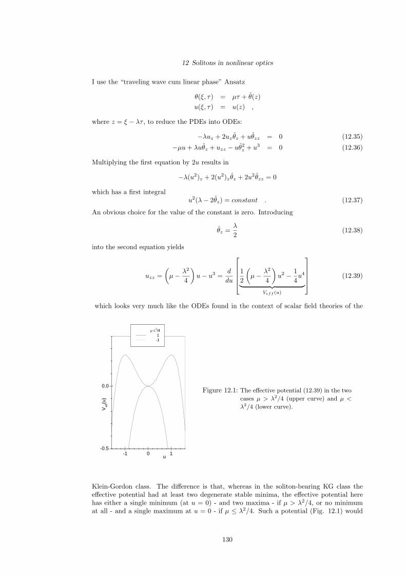
12 Solitons in nonlinear optics
I use the “traveling wave cum linear phase” Ansatz
θ(ξ, τ) = µτ + θ(z)u(ξ, τ) = u(z) ,
where z = ξ − λτ , to reduce the PDEs into ODEs:
−λuz + 2uz θz + uθzz = 0 (12.35)
−µu + λuθz + uzz − uθ2z + u3 = 0 (12.36)
Multiplying the first equation by 2u results in
−λ(u2)z + 2(u2)z θz + 2u2θzz = 0
which has a first integralu2(λ− 2θz) = constant . (12.37)
An obvious choice for the value of the constant is zero. Introducing
θz =λ
2(12.38)
into the second equation yields
uzz =(
µ− λ2
4
)u− u3 =
d
du
12
(µ− λ2
4
)u2 − 1
4u4
︸ ︷︷ ︸Veff (u)
(12.39)
which looks very much like the ODEs found in the context of scalar field theories of the
-1 0 1-0.5
0.0
Vef
f(u)
u
µ-λ2/4 1 -1
Figure 12.1: The effective potential (12.39) in the two
cases µ > λ2/4 (upper curve) and µ <
λ2/4 (lower curve).
Klein-Gordon class. The difference is that, whereas in the soliton-bearing KG class theeffective potential had at least two degenerate stable minima, the effective potential herehas either a single minimum (at u = 0) - and two maxima - if µ > λ2/4, or no minimumat all - and a single maximum at u = 0 - if µ ≤ λ2/4. Such a potential (Fig. 12.1) would
130

12 Solitons in nonlinear optics
of course be entirely unphysical in the context of field theory, because of the instability atlarge displacements. Here there is no such physical restriction. A soliton-like solution canoccur as long as there is a single, locally stable minimum; it will lead the system from thelocal minimum out to either one of the maxima and back to to the local minimum. Notethat this implies that, in the first integral of (12.39),
u2z = 2Veff (u) + const
the constant vanishes. This leads to the formal second integral
z − z0 = ±∫
du1√
2V (u)
and the bounded solutions
u(z) = ± κ sechκ(z − z0)√
2(12.40)
where I have used the more appropriate constant
κ = +
√2
(µ− λ2
4
).
Note that since I have up to now introduced two arbitrary constants (in addition to thearbitrary phase z0), I can take any value of κ > 0 and λ; µ will then have the fixed (andpositive) value
µ =κ2
2+
λ2
4.
To conclude, I note that from (12.38)
θ =λ
2z + θ0 (12.41)
where θ0 is an arbitrary phase. Collecting terms, and returning to the original space-timevariables,
u(ξ, τ) = ± κ sechκ(ξ − λτ − z0)√
2(12.42)
θ(ξ, τ) =λ
2
ξ −
(λ
2− κ2
λ
)τ
+ θ0 (12.43)
Note that envelope amplitude and phase propagate with different velocities, ve = λ andvph = λ/2− κ2/λ, respectively.
131

13 Solitons in Bose-EinsteinCondensates
13.1 The Gross-Pitaevskii equation
Starting point: Gross-Pitaevskii equation [33, 34] for the weakly interacting Bose gas (par-ticles of mass m):
ih∂
∂tΨ0 =
− h2
2m∇2 + Vext(~r) + g|Ψ0|2
Ψ0 (13.1)
where
• Ψ0(~r, t) is the condensate wave function; the condensate density is then
n(~r) = |Ψ0|2 .
• g = 4πh2a/m the coupling constant, with
• a the s-wave scattering amplitude (low-energy characteristic of the effective potential).
• the external potential, typically of the form
Vext(~r) = α(x2 + y2) + λz2 (13.2)
describes a cylindrically symmetric magnetic trap.
In the limit λ ¿ α, I look for solutions which depend only on z; these must satisfy
ih∂
∂tΨ0 =
− h2
2m
∂2
∂z2+ g|Ψ0|2
Ψ0 (13.3)
which I recognize as the nonlinear Schrodinger equation. A useful quantity is the character-istic length defined by
ξ2 =h2
2mgn=
18πan
(13.4)
where n is the average condensate density.
13.2 Propagating solutions. Dark solitons
I look for propagating solutions of the form
Ψ0 =√
ne−iµt/hφ(ζ)
whereζ =
z − vt
ξ
and µ = gn is the chemical potential. I will treat the case g > 0 (repulsive interaction).
132
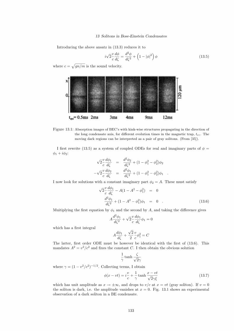
13 Solitons in Bose-Einstein Condensates
Introducing the above ansatz in (13.3) reduces it to
i√
2v
c
dφ
dζ=
d2φ
dζ2+
(1− |φ|2
)φ (13.5)
where c =√
gn/m is the sound velocity.
Figure 13.1: Absorption images of BEC’s with kink-wise structures propagating in the direction of
the long condensate axis, for different evolution times in the magnetic trap, tev. The
moving dark regions can be interpreted as a pair of gray solitons. (From [35]).
I first rewrite (13.5) as a system of coupled ODEs for real and imaginary parts of φ =φ1 + iφ2:
√2v
c
dφ1
dζ=
d2φ2
dζ2+ (1− φ2
1 − φ22)φ2
−√
2v
c
dφ2
dζ=
d2φ1
dζ2+ (1− φ2
1 − φ22)φ1 .
I now look for solutions with a constant imaginary part φ2 = A. These must satisfy√
2v
c
dφ1
dζ−A(1−A2 − φ2
1) = 0
d2φ1
dζ2+ (1−A2 − φ2
1)φ1 = 0 . (13.6)
Muitiplying the first equation by φ1 and the second by A, and taking the difference gives
Ad2φ1
dζ2+√
2v
c
dφ1
dζφ1 = 0
which has a first integral
Adφ1
dζ+√
22
v
cφ2
1 = C
The latter, first order ODE must be however be identical with the first of (13.6). Thismandates A2 = v2/c2 and fixes the constant C. I then obtain the obvious solution
1γ
tanhζ√2γ
where γ = (1− v2/c2)−1/2. Collecting terms, I obtain
φ(x− vt) = iv
c+
1γ
tanhx− vt√
2γξ(13.7)
which has unit amplitude as x → ±∞, and drops to v/c at x = vt (gray soliton). If v = 0the soliton is dark, i.e. the amplitude vanishes at x = 0. Fig. 13.1 shows an experimentalobservation of a dark soliton in a BE condensate.
133

14 Unbinding the double helix
14.1 A nonlinear lattice dynamics approach
14.1.1 Mesoscopic modeling of DNA
Background: thermodynamic phase transitions
Transitions between different states of matter (e.g. the transition from the paramagnetic tothe ferromagnetic phase, or the liquid-gas transition) are reflected in singularities of the ther-modynamic functions (free energy, entropy etc). The modern theory of critical phenomenadeveloped by Fisher, Kadanoff and Wilson during the 1960’s and 70’s has demonstrated thatthe essential features of such mathematical singularities depend only on a few “relevant”degrees of freedom of the underlying Hamiltonian. As a consequence, substantial effort hasbeen made by researchers in developing and studying appropriately reduced descriptions,“minimal” models of many complex phenomena related to transformations between differentstates of matter.
Figure 14.1: Melting of poly(dI)-poly(dC) (after [36]).
Experiment suggests DNA denaturation is a sharp phase transition
The thermal denaturation of DNA (also known as DNA melting) consists of the unbindingof the double helix into the two component strands. There is no breaking of covalent bondsalong the chain, and the transition is in principle reversible. In the case of DNA chainswhich are long (of the order of N ≈ 104 base pairs) and homogeneous (i.e. all base pairsare identical), the transition, as observed by the difference in UV absorption spectra, canbe very sharp (Fig. 14.1). It is then perfectly reasonable to assume that the underlyingphenomenon would be an exact phase transition in the thermodynamic limit N → ∞ andattempt to model it accordingly.
134
14 Unbinding the double helix
Mesoscopic modeling: 1 degree of freedom per base pair
A reduced, mesoscopic description of DNA consists of assigning a single continuous, “trans-verse” degree of freedom yn to the nth base pair, corresponding to the distance betweenthe two bases which comprise the pair. The energy related to this degree of freedom has itsphysical origin in the hydrogen bonds which are responsible for pair binding. Accordingly,it is modeled by a Morse potential
V (y) = D(e−ay − 1)2
where D is an average measure of the binding energy and 1/a a length which characterizes therange of the hydrogen bonding. The tendency of successive base pairs to “stack” (“stacking”interaction) can be modeled by assuming that they are bound together by springs. Forsimplicity, I will assume these springs to be harmonic.
The total Hamiltonian will then be of the form [37]
H =∑
n
[p2
n
2µ+
12µω2
0(yn+1 − yn)2 + V (yn)]
, (14.1)
where µ is the reduced mass corresponding to the base pair, pn = µyn is the canonicalmomentum conjugate to yn and µω2
0 a measure of the strength of the stacking interaction.
Note that this minimal modeling makes no reference to the helical structure of themolecule. Although generalizations to that effect have been formulated, it should be bornein mind that this type of modeling makes no attempt to describe structural details of theDNA molecule. Its scope begins and ends with capturing essential observed macroscopicfeatures at and very near the denaturation point.
14.1.2 Thermodynamics
The classical thermodynamics of H is described by the canonical partition function
Z =∫ N∏
n=1
dpndyne−βH . (14.2)
which factorizes into a product of Gaussian integrals over the momentum variables,
ZK = (2πµ/β)N/2 , (14.3)
and a nontrivial configurational part
ZP =∫ (
N∏n=1
dyn
)T (y1, y2) · · ·T (yN−1, yN )T (yN , yN+1) , (14.4)
where
T (x, y) = e−β
[µω2
02 (y−x)2+V (x)
]. (14.5)
The transfer integral formalism: definitions and notation
Consider the eigenvalue problem defined by the asymmetric kernel T (the kernel can be easilysymmetrized but need not be so; in fact, working with the asymmetric kernel is technically
135

14 Unbinding the double helix
advantageous in examining the validity of some approximations, cf. below):∫ ∞
−∞dy T (x, y) ΦR
ν (y) = ΛνΦRν (x) (14.6)
∫ ∞
−∞dy T (y, x) ΦL
ν (y) = ΛνΦLν (x) , (14.7)
where left and right eigenstates have been assumed to be normalized; note that the normal-ization integral is
∫dxΦL
ν (x)ΦRν (x). Orthogonality∫ ∞
−∞dx ΦL
ν (x) ΦRν′(x) = δνν′ (14.8)
and completeness ∑ν
ΦLν (x) ΦR
ν (y) = δ(x− y) (14.9)
relationships are assumed to hold. I will further use the notation
Λν = e−βεν (14.10)
(sensible as long as the eigenvalues are nonnegative).
Relationship between Z and the spectrum of T
The integrand of (14.4), as written down has a problem: it includes a reference to thedisplacement yN+1 of the N + 1st particle, which has not yet been defined. For a largesystem, this is best remedied by means of periodic boundary conditions (PBC), i.e. bydemanding that yN+1 = y1. Alternatively, the integration may be extended to one morevariable, dyN+1, with the simultaneous introduction of a factor δ(yN+1− y1) to take care ofPBC. This however is the same as the sum in the left-hand-side of (14.9). I then obtain
ZP =∑
ν
∫dy1 · · · dyN+1ΦL
ν (y1)︸ ︷︷ ︸ T (y1, y2) · · ·T (yN , yN+1)ΦRν (yN+1)︸ ︷︷ ︸ . (14.11)
The braces make clear that I can perform the integral over dyN+1 and obtain a factorΛνΦR
ν (yN+1), using the defining property of right-hand eigenfunctions. The process can berepeated N times, each time giving a further factor Λν and a right eigenfunction with anargument whose index is smaller by one. At the end, I am left with
ZP =∑
ν
∫dy1ΦL
ν (y1)ΛNν ΦR
ν (y1) =∑
ν
ΛNν . (14.12)
In the thermodynamic limit, ZP is dominated by the largest eigenvalue Λ0 or, equivalently,the lowest ε0:
limN→∞
1N
ln ZP = lnΛ0 = −βε0 (14.13)
The order parameter
< yi > =1
ZP
∫dy1 · · · dyNT (y1, y2) · · ·T (yi−1, yi)yi
T (yi, yi+1) · · ·T (yN , yN+1)
≡ 1ZP
∑ν
∫dy1 · · · dyN+1ΦL
ν (y1) T (y1, y2) · · ·T (yi−1, yi)︸ ︷︷ ︸i−1
yi
T (yi, yi+1) · · ·T (yN , yN+1)︸ ︷︷ ︸N−i+1
ΦRν (yN+1) , (14.14)
136

14 Unbinding the double helix
after insertion of a complete set of states (cf. above); the braces denote the number oftimes I can perform an integration and obtain, respectively, a right eigenfunction with anargument smaller by one, or a left eigenfunction with an argument larger by one, as well asa factor Λν . The remaining integral must be performed explicitly:
< yi > =1
ZP
∑ν
ΛNν Mνν
≈ M00 (14.15)
where the second line is exact in the thermodynamic limit, and I have used the abbreviation
Mνµ =∫ ∞
−∞dyΦL
ν (y)yΦRµ (y) . (14.16)
The spectrum of T: Gradient-expansion approximation; analogy with quantummechanics
Suppose that the displacement field does not change appreciably over a lattice constant.This is certainly reasonable at low temperatures. Note that this does not exclude largedisplacements per se. Nonlinearity is explicitly allowed, but the displacement field must besmooth. The assumption is certainly reasonable at low temperatures.
I set y = x + z, ΦR → φ and rewrite (14.6) as
e−β[εν−V (x)]φν(x) =∫ +∞
−∞dz e−
12 βµω2
0z2
φν(x) + zφ′ν(x) +12z2φ′′ν(x)
=[
2π
βµω20
]1/2 φν(x) +
12βµω2
0
φ′′ν(x)
(14.17)
where higher terms in the gradient expansion have been neglected and the Gaussian integralshave been performed; this is meaningful as long as the width of the Gaussians is smallerthan the range of the Morse potential, i.e.
βµω20/a2 > 1 . (14.18)
The factor in front of the r.h.s. of (14.17) can be absorbed in the eigenvalue by definingεν = εν + 1/(2β)] ln[2π/(βµω2
0)]. Now, for many practical purposes, when it comes tocalculating matrix elements, the relevant magnitude of ε − V (x) is D, the depth of theMorse well (or some other characteristic energy in the case of another potential). The keyto this statement is that one does not need to consider large negative values of x, whereV (x) is huge, because at such x, both the exact eigenfunction Φ and its approximation φcan be expected to be negligible. If then βD ≤ 11 it is reasonable to expand the exponentialand keep only the first term. Dividing both sides by β, I obtain a Schrodinger-like equation,
− 12µ(βω0)2
φ′′ν(x) + [V (x)− εν ]φν(x) = 0 . (14.19)
Before continuing the discussion of (14.19) and its properties, I pick up the bits and pieces(cf (14.2), (14.3), (14.13) ) of the thermodynamic free energy (per site)
f = − 1βN
ln(ZKZP ) ≡ − 1β
ln(
2π
βω0
)+ f , (14.20)
1Note that, in connection with (14.18), this defines a temperature window D < kBT < µω20/a2 for the
validity of the overall approximation scheme.
137

14 Unbinding the double helix
where f = ε0. The first term in (14.20) is the free energy of the small oscillations (transversephonons in this context). It is a term smooth in temperature (constant specific heat!) andtherefore irrelevant to any phase transition. Any nontrivial physics is hidden in the secondterm, which is identical with the the smallest eigenvalue of (14.19).
A couple of comments are in order. First, (14.19) would be a literal (i.e. quantum-mechanical) Schrodinger equation, if I substituted 1/(βω0) by h. I will come back to thatpoint. Second, I can get a dimensionless potential (and eigenvalue) by dividing both sidesof (14.19) by D. In other words, the relevant dimensionless parameter is
δ2 =
2µa2h2 · D (quantum mechanics)
2µβ2ω20
a2 · D (statistical mechanics).(14.21)
In terms of δ, the bound state spectrum of (14.19) is given [38] by
εn
D= 1−
[1− n + 1/2
δ
]2
n = 0, 1, ..., int(δ − 1/2) . (14.22)
There is at least one bound state if δ > 1/2. For 1 ≥ δ > 1/2 there is exactly one boundstate. And if δ becomes equal to, or smaller than 1/2, there is no bound state at all. Thevalue δc = 1/2 is ”critical”. In quantum mechanical language, if a particle has a masswhich is lighter than a critical mass µc = h2a2/(8D), it cannot be confined in the Morsewell. Quantum fluctuations will drive it out2.
Thermodynamic free energy
In the context of statistical mechanics, δc corresponds, via (14.21), to a critical temperatureTc = 2(ω0/a)
√2µD. The free energy is given by
f
D=
1 T > Tc
1−(1− T
Tc
)2
T < Tc ,
(14.23)
where in the upper line I have made use of the fact that the bottom of the continuum partof the spectrum is at ε = D. The free energy f is non-analytic at T = Tc, where its secondderivative is discontinuous (i.e. there is a jump in the specific heat). This corresponds to asecond order transition, according to the Ehrenfest classification scheme3.
The order parameter. DNA melting as a thermodynamic instability
In order to gain some further insight into the physics involved4 it is useful to examine theaverage displacement (14.15), determined by the ground-state (GS) eigenfunction
φ0(x) = e−ζ/2 ζδ−1/2 (14.24)2This is a general property of asymmetric one-dimensional wells; symmetric wells will support a particle
in a bound state, no matter how low its mass.3Note that the term “second order” is meant literally in this case, not just as a metaphor for the absence
of a latent heat (for which the term ”continuous transition” would be appropriate).4The mathematical analogy between the behavior of the spectral gap which occurs in a point (d = 0)
system and the singularity in the free energy of a classical chain (d = 1) is an example of a deeper analogywhich relates quantum to thermal fluctuations; the formal correspondence h ↔ 1/(βω0) manifests a far-reaching analogy between d-dimensional quantum mechanics and (d +1)-dimensional classical statisticalmechanics. The analogy is most fruitful at d = 1, because of the interplay and the richness of exactavailable results which based either in the transfer-matrix approach of 2-dimensional classical statisticsor on the Bethe-Ansatz developed for 1-d quantum spin systems.
138

14 Unbinding the double helix
where ζ = 2δe−ax. It is straightforward to see that, as T approaches Tc from below, theeigenfunction extends towards larger and larger positive values of x:
φ0(x) ∝ e−λx (14.25)
where
λ =1
δ − δc(14.26)
is a (transverse) characteristic length which measures the spatial extent of the GS eigen-function. As a consequence, we can estimate that < y >, which is dominated by the largevalues of the argument, will also behave as
< y >∼ (δ − δc)−1 ∼(
1− T
Tc
)−1
. (14.27)
As the critical temperature is approached from below, particles cease to be confined to theminimum of the Morse well. They perform larger and larger excursions to the flatter partof the potential. At Tc the transition is complete; the average transverse displacement isinfinite. Particles move, on the average, on the flat top of the Morse potential. Unwinding(“melting”) of the DNA has occurred.
In the language of critical phenomena < y > is the order parameter. In ordinary phasetransitions, where one goes from an ordered to a disordered phase, the order parameter mvanishes at the transition point, i.e m ∝ (Tc−T )β with a positive critical exponent β5. DNAmelting is really an instability - rather than an “order-disorder” transition. It is thereforenot surprising that the corresponding critical exponent β extracted from (14.27) is negative(-1).
Experimental data on DNA denaturation do not deliver < y > directly. The “experimentalorder parameter” is the helical fraction, i.e. the probability that a given base pair is stillbound; technically one uses an (instrumentation-dependent) cutoff y0 and measures P (y >y0, T ). For the model presented here, this function approaches zero smoothly (linearly) asT → Tc, independently of the choice of y0.
14.2 Nonlinear structures (domain walls) and DNA melting
In discussing how adsorbed atoms arrange themselves on a substrate, we examined a num-ber of possibilities: a uniform structure, commensurate with the substrate, and a solitonlattice. We found that the commensurate-incommensurate phase transition occurred whenthe mismatch between the competing lattice periodicities made the soliton lattice energet-ically favored. The DNA denaturation - as described within the model Hamiltonian (14.1)- is a thermal, not a parametric instability. Nonetheless, it will prove useful to examine theexistence and properties [39] of competing nonlinear structures of (14.1).
In this section I will use dimensionless variables ayn → yn; the energy will be measuredin units of D. The total potential energy will then be
Φ =N∑
n=0
[1
2R(yn+1 − yn)2 + V (yn)
](14.28)
where R = D/(Ka2) is a dimensionless coupling constant.
5not to be confused with the inverse temperature; this is the standard notation of critical phenomena
139
14 Unbinding the double helix
14.2.1 Local equilibria
Definition
Local equilibria are defined by static solutions of the equations of motion, i.e. by extrema
∂Φ∂yn
= 0 ∀n. (14.29)
of the total potential energy. Their spatial patterns, for a given boundary condition y0 =0, yN+1 = L are described by a second-order difference equation
yn+1 − 2yn + yn−1 + RV ′(yn) = 0 ∀n = 1, · · ·N . (14.30)
Fixed point
There is only one fixed pointyn = 0 ∀n
of the map. Note however that it is compatible only with the boundary condition L = 0.Note further that the energy associated with the fixed point configuration is zero.
Stability criteria
The stability of equilibria is governed by the spectra of the corresponding N × N Hessianmatrix
hij =∂2Φ
∂yi∂yj(14.31)
where the derivative is evaluated at the extrema defined by (14.30). Let Λν , ν = 1, · · · , Ndenote the eigenvalues of the matrix h. If, for a given extremum, the eigenvalues are allpositive, then the extrema is a local minimum. If they are all negative it is a local maximum.If some are negative and some are positive it is a local saddle point. I will not discuss theinteresting marginal case where an eigenvalue vanishes, since it does not arise in the contextof this particular problem.
Picturing and classifying equilibria
What do these equilibria look like? A picture can be given by looking at the full set ofsolutions of (14.30), without fixing the value of L, and then choose the ones that correspondto the boundary condition yN+1 = L. This can be done by noting that (14.30) for unspecifiedL is equivalent to all realizations of the two-dimensional map
pn+1 = pn + RV ′(yn)yn+1 = yn + pn+1 , (14.32)
where n = 1, · · · , N , y1 = p1 + y0, y0 = 0 and p1 is unspecified. The set of all orbits of themap thus derived is shown in Fig (14.2). Note that there are two kinds of orbits. Stable ones(drawn with full points) and saddles (drawn with open points), where all but one eigenvaluesof the Hessian are positive. It is then possible to isolate those orbits which correspond to agiven L. They are shown in Fig. (14.2.1). We note that they start off at a value very closeto zero, remain there for a few sites, and then suddenly “take” off with a constant linearslope. The equilibria pictured here represent in some sense “interpolations” - or domainwalls (DWs - between the bound (y ≈ 0) and the unbound (y À 1) phase.
140

14 Unbinding the double helix
0 1 2 3 4 5 60
10
20
30
40
50
4 5
43
44
45
y
p
Figure 14.2: The unstable manifold of the FP
of the map (14.32) for R = 10.1
and N = 28. Black squares belong
to stable equilibria, red open circles
belong to unstable equilibria. The
horizontal line at y = 44 demon-
strates the multivaluedness of the
manifold as a function of y (4 sta-
ble and 3 unstable equilibria with
that value of y; details in the in-
set). The vertical lines are drawn
at pmin and pmax, the minimal and
maximal asymptotic slopes of DWs
(from [39].
0 5 10 15 20 25 30
0
20
40
60
80
4.0 4.5 5.0 5.535.5
36.0
36.5
37.0
E
yn
n
p
Figure 14.3: The 8 stable equilibria correspond-
ing to N = 28, y0 = 0, yN+1 = L =
80. Not shown are 7 unstable equi-
libria enmeshed between the stable
ones. Inset: total energies for both
stable (black squares) and unstable
(red open circles) equilibria. The
continuous curve corresponds to a
theoretical estimate which does not
distinguish between stable and un-
stable equilibria (cf. text); (from
[39]).
Configuration of lowest energy for a given L 6= 0.
For a given slope p of the unbound segment, there are L/p unbound sites. The excess energyfrom them is
E(p) =(
p2
2R+ 1
)L
p
and has a minimum at p = p∗ = (2R)1/2. Thus, the minimum energy required to create aDW at a given L is
E∗(L) =(
2R
)1/2
L . (14.33)
As long as this energy is not available, the system will, if left to itself, prefer the equilibriumavailable at the fixed point. In order to maintain the transverse displacement L, one mustapply an external force
f =dE∗(L)
dL=
(2R
)1/2
. (14.34)
This is exactly what happens in single-molecule experiments which achieve mechanical DNAdenaturation or, as commonly called, DNA unzipping.
141

14 Unbinding the double helix
0 10 20 30
0
1
2
Λν
ν
N=32, L=100 0 *
Figure 14.4: Eigenvalue spectra of the Hessians
for (i) the fixed point (open squares)
and (ii) the DW with minimal en-
ergy (open circles) for L = 100. In
both cases N = 32. The DW’s
spectrum consists of bands of opti-
cal and acoustic phonons, localized
respectively in the bound and un-
bound portions of the chain, and a
single local mode in the gap; both
bands are well described (to order
O(1/L)) by the corresponding free
phonon dispersion curves (dotted);
(from [39]).
14.2.2 Thermodynamics of domain walls
At any finite temperature, we will have to consider the competition of the two possiblestructures: the one corresponding to the fixed point, and the corresponding to the DW withthe least energy. Strictly speaking, in the latter case we are considering the totality of allpossible values of L.
Free energy associated with a given minimum
For small displacements around any given local minimum yn, i.e.
yn = yn + un
the total potential energy will be given, to quadratic order in the displacements, by
Φ(u) ≈ E(y) +12
∑
i,j
hijuiuj ,
where E(y) is the energy of the local minimum.
The associated configurational part of the partition function will be
Z(y) = e−βE(y)
∫ ∞
−∞
(N∏
m=1
dum
)e− β
2
∑i,j
hijuiuj
= e−βE(y)N∏
ν=1
(2π
βΛν
)1/2
(14.35)
where the product runs over all eigenvalues of the Hessian. Note that the eigenvalues must bestrictly positive, not just nonnegative. The free energy associated with any given minimumwill then be
F (y) = −T ln Z(y) = E(y)− T
2
N∑ν=1
ln(
2π
βΛν
)(14.36)
Comparison of free energies
The spectra of (i) the fixed point and (ii) the stable DW with the minimal energy at somefinite L are shown in Fig. 14.2.2.
142

14 Unbinding the double helix
Now consider the difference in free energies between the DW with the minimal energy atsome finite L and the fixed point
∆F (L) = E∗(L)− T
2
N∑ν=1
ln(
Λ0ν
Λ∗ν
)(14.37)
where the star in the superscript denotes the DW and the 0 the fixed point.
The second term represents the difference in entropies. Formation of the DW generates again in entropy. The quantity
12
N∑ν=1
ln(
Λ0ν
Λ∗ν
)≡ L
p∗σ(R)
is generally proportional to the number L/p∗ of unbound sites. The extra entropy comesexclusively from the unbound part. It is due to the fact that the acoustic phonons whichlive in the unbound region have lower frequencies than the optical phonons which live in thebound state defined by fixed point.
Combining terms, the difference in free energy can be written as
∆F (L) = [2− Tσ(R)]L
p∗(14.38)
which becomes zero atTc(R) =
2σ(R)
(14.39)
and negative at higher temperatures. Thus, if the temperature is raised beyond Tc(R) a DWof any length can be formed spontaneously - since it generates a net gain in free energy.Denaturation can occur spontaneously.
Alternatively, we may look at the derivative
p =dF (L)
dL= [2− Tσ(R)]
1p∗
(14.40)
which represents the unzipping force at a finite temperature T . Spontaneous thermal de-naturation is, in this sense, equivalent to the vanishing of the unzipping force.
For not too large values of R, the proportionality constant is
σ(R) = ln(√
R/2 +√
1 + R/2)
. (14.41)
In the continuum limit, R ¿ 1, this gives a Tc = 2(2/R)1/2, which is exactly the criticaltemperature found in Section 14.1.2.
In summary, what I have presented in this lecture is an alternative picture of the DNAinstability, based on the underlying, competing nonlinear equilibrium structures (domainwalls vs. fixed point). The results suggest that the domain wall, via the entropic gain itgenerates, can overcome the energetic cost of its production. In other words, spontaneousformation of a DW at the instability temperature is what really “drives” DNA denaturation.
143

15 Pulse propagation in nerve cells: theHodgkin-Huxley model
15.1 Background
The physics of electric pulse propagation in nerve cells [40] has a long and interesting history.Helmholtz measured the signal velocity on a frog’s sciatic nerve in 1850. Bernstein succeededshortly thereafter (1868) in detecting the complete shape of the pulse, the action potentialV (t) as a function of time. The concept of a nerve cell, or neuron as an independentfunctional unit was established through extensive anatomical studies by Ramon y Cajal inthe beginning of the twentieth century. Typically, a neuron (Fig. 15.1) consists of an inputcollecting part with a dendritic structure (dendrites), a cell nucleus, and an output fiber(axon) which transports and relays the signals. The membrane of the nerve cell, whose
Figure 15.1: A nerve cell.
existence was experimentally confirmed by Fricke in the 1920’s, is permeable to K+ andNa+ ions. If the nerve is at rest, the inner and outer surfaces of the membrane carry,respectively, net negative and positive electric charges. The corresponding resting potential(Ruhepotential) Vin − Vout is of the order of 50mV .
15.2 The Hodgkin-Huxley model
A significant breakthrough in our understanding of pulse propagation in nerve cells is dueto experimental and theoretical work done by Hodgkin and Huxley (HH) in the 1950’s onthe giant1 axon of the Atlantic squid (Loligo pealei).
1The diameter of the squid’s axon is of the order of 1.5mm, which is about 50 times as thick as that ofmost animals, including humans.
144
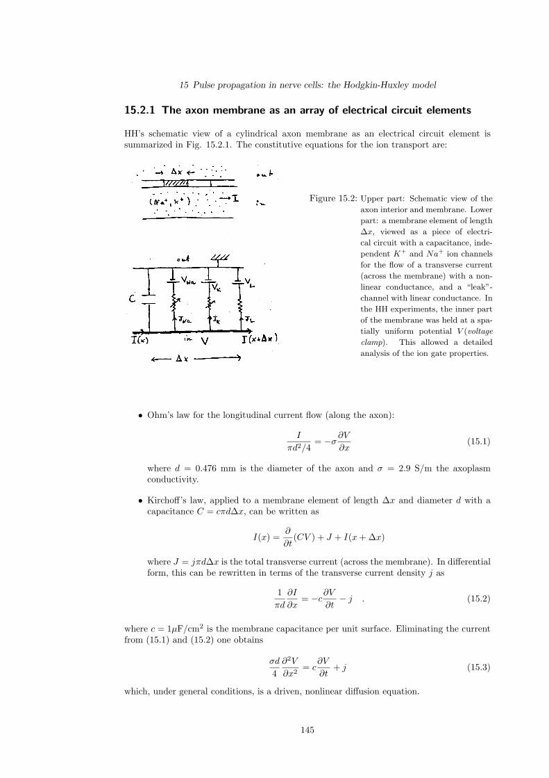
15 Pulse propagation in nerve cells: the Hodgkin-Huxley model
15.2.1 The axon membrane as an array of electrical circuit elements
HH’s schematic view of a cylindrical axon membrane as an electrical circuit element issummarized in Fig. 15.2.1. The constitutive equations for the ion transport are:
Figure 15.2: Upper part: Schematic view of the
axon interior and membrane. Lower
part: a membrane element of length
∆x, viewed as a piece of electri-
cal circuit with a capacitance, inde-
pendent K+ and Na+ ion channels
for the flow of a transverse current
(across the membrane) with a non-
linear conductance, and a “leak”-
channel with linear conductance. In
the HH experiments, the inner part
of the membrane was held at a spa-
tially uniform potential V (voltage
clamp). This allowed a detailed
analysis of the ion gate properties.
• Ohm’s law for the longitudinal current flow (along the axon):
I
πd2/4= −σ
∂V
∂x(15.1)
where d = 0.476 mm is the diameter of the axon and σ = 2.9 S/m the axoplasmconductivity.
• Kirchoff’s law, applied to a membrane element of length ∆x and diameter d with acapacitance C = cπd∆x, can be written as
I(x) =∂
∂t(CV ) + J + I(x + ∆x)
where J = jπd∆x is the total transverse current (across the membrane). In differentialform, this can be rewritten in terms of the transverse current density j as
1πd
∂I
∂x= −c
∂V
∂t− j . (15.2)
where c = 1µF/cm2 is the membrane capacitance per unit surface. Eliminating the currentfrom (15.1) and (15.2) one obtains
σd
4∂2V
∂x2= c
∂V
∂t+ j (15.3)
which, under general conditions, is a driven, nonlinear diffusion equation.
145

15 Pulse propagation in nerve cells: the Hodgkin-Huxley model
15.2.2 Ion transport via distinct ionic channels
According to HH, the transverse current per unit length consists of distinct ionic components,and a “leakage” current
j = jNa + jK + jL (15.4)
with
jNa = GNa gNa (V − VNa)jK = GK gK (V − VK)jL = GL (V − VL) , (15.5)
where VNa = 115 mV , VK = −12 mV are the electrochemical potentials for Na and K ionsrespectively, and VL = 10.6 mV is adjusted so that the total current j vanishes if V = 0.Note that this condition really corresponds to the rest state, i.e. V = Vin − Vout + 65mV .The electrochemical potentials of the squid axon are fairly typical: the corresponding valuesfor the frog’s sciatic nerve are VNa = 122mV , VK ≈ 0mV . The Gi’s are linear conductances,GNa = 120 mS cm−2, GK = 36 mS cm−2, GL = 0.3 mS cm−2.
Finally, the gi’s are nonlinear dimensionless functions of the potentials, to be discussedbelow.
15.2.3 Voltage clamping
In order to study the details of nonlinear transport, HH developed an experimental technique,called space clamping. The technique consisted of piercing the axon with a thin metallicelectrode, so that the inside of the membrane could be held at a spatially uniform potential.In this case, using (15.3),(15.4) and (15.5), one obtains
c∂V
∂t= GNa gNa (V − VNa) + GK gK (V − VK) + GL (V − VL) . (15.6)
Voltage clamping was a further technical development which made it possible to controlthe uniform voltage at any desired level. Clamping was a major conceptual breakthroughin the electrophysics of nerve cells because it facilitated a detailed analysis of experimentaldata and made possible the extraction of crucial information on the unknown functions gi.
15.2.4 Ionic channels controlled by gates
The experimental findings of HH led them to conclude that the two ionic channels arecontrolled by gates. Moreover, a phenomenological description of the data could be only beachieved by postulating the existence of different types of gates. Thus
gK = n4 (15.7)gNa = m3h (15.8)
where m,n, h ∈ [0, 1] are gating functions.
Gating functions
The value of any gating function p corresponds to the probability that the correspondinggate is in its “open” state. The time evolution of any gating function is governed by afirst-order ordinary differential equation
dp
dt= α(1− p)− βp = −p− p0
τ(15.9)
146

15 Pulse propagation in nerve cells: the Hodgkin-Huxley model
-50 0 50 100
0.0
0.5
1.0
-50 0 50 1000.1
1
10
100
n0
m0
h0
V (mV)
τn
-1
τm
-1
τh
-1
mse
c-1
V
Figure 15.3: The HH gating functions at equilibrium. n0
and m0 are of the activation type, h0 is of
the deactivation type. Inset: the inverse re-
laxation times which correspond to the gating
functions. Note that the m-gate is consider-
ably faster than either the n or the h gates.
where αdt is the probability that the closed gate will open within the time dt, and βdt theprobability that the open gate will close during the same time interval. Both α and β are, ingeneral, nonlinear functions of the membrane potential V . The second form of the equation,where the new parameters are defined as
1τ
= α + β
p0 =1
1 + βα
, (15.10)
shows clearly that the gating function approaches an equilibrium value p0(V ) for any givenmembrane potential within a characteristic time τ(V ).
Gates are classified as either of the activation type, if
limV→∞
p(V ) = 1 ,
or of the deactivation type, iflim
V→∞p(V ) = 0 .
HH gate parameters
The gating function n which controls the flow of K+ ions is of the activation type, with
αn =0.01(10− V )
e10−V
10 − 1, βn = 0.125e−
V80 . (15.11)
Here αn and βn are measured in msec−1, V in mV.
The flow of Na+ is controlled by both an activation-type gate m, with
αm =0.1(25− V )
e25−V
10 − 1, βm = 4e−
V18 , (15.12)
and a deactivation-type gate h, with
αh = 0.07e−V20 , βh =
1
e30−V
10 + 1. (15.13)
The corresponding values of the gating functions at equilibrium are shown in Fig. 15.2.4.
147

15 Pulse propagation in nerve cells: the Hodgkin-Huxley model
15.2.5 Membrane activation is a threshold phenomenon
The solutions of the HH equations under space-clamping conditions for a variety of initialmembrane potentials are shown in Fig. 15.4. A spike always forms, provided that the initialstimulus is above a certain threshold ∼ 6.5mV. The spike amplitude and width are roughlyindependent of the initial stimulus.
0 2 4 6 8 10 12
-20
0
20
40
60
80
100
120
V (
mV
)
t (msec)
V(0) (mV) 90 60 30 15 10 7 6 5
Figure 15.4: The membrane potential as a function of time
for a variety of initial stimuli. Note that a
spike will always form if the initial stimulus
is above a certain threshold; amplitude and
width of the spike are roughly independent of
the strength of the stimulus. The threshold
lies between 6 and 7 mV.
15.2.6 A qualitative picture of ion transport during nerve activation
On the basis of the HH model, the following qualitative picture emerges for the temporalevolution of the action potential during nerve activation (cf. Fig. 15.2.6:
• At zero membrane potential, m0(0) = 0.053, h0(0) = 0.596; the product m3h is verysmall, hence the Na+ current will be very small. Since n0(0) = 0.318, the K+ currentwill also be small.
• As the membrane voltage is turned on, the m-gate of the Na+ channel is rapidlyactivated (cf. Fig. 15.2.4), within a characteristic time 0.2 − 0.4 msec. Sodium ionsflow into the axon.
• As V approaches the electrochemical potential of sodium, VNa = 115 mV , the influxof sodium ions becomes small.
• At high values of V the h-gate becomes deactivated. The Na+ channel closes withina characteristic relaxation time of 1− 8 msec.
• While this happens, the slower potassium gate n becomes activated, with a charac-teristic time of 2 − 5 msec. K+ ions begin to flow out of the axon. The membranedepolarizes.
15.2.7 Pulse propagation
It is now possible to look for propagating solutions of the nonlinear diffusion equation (15.3),i.e. solutions of the form V (x − vt); since electrodes are usually placed at a fixed point in
148
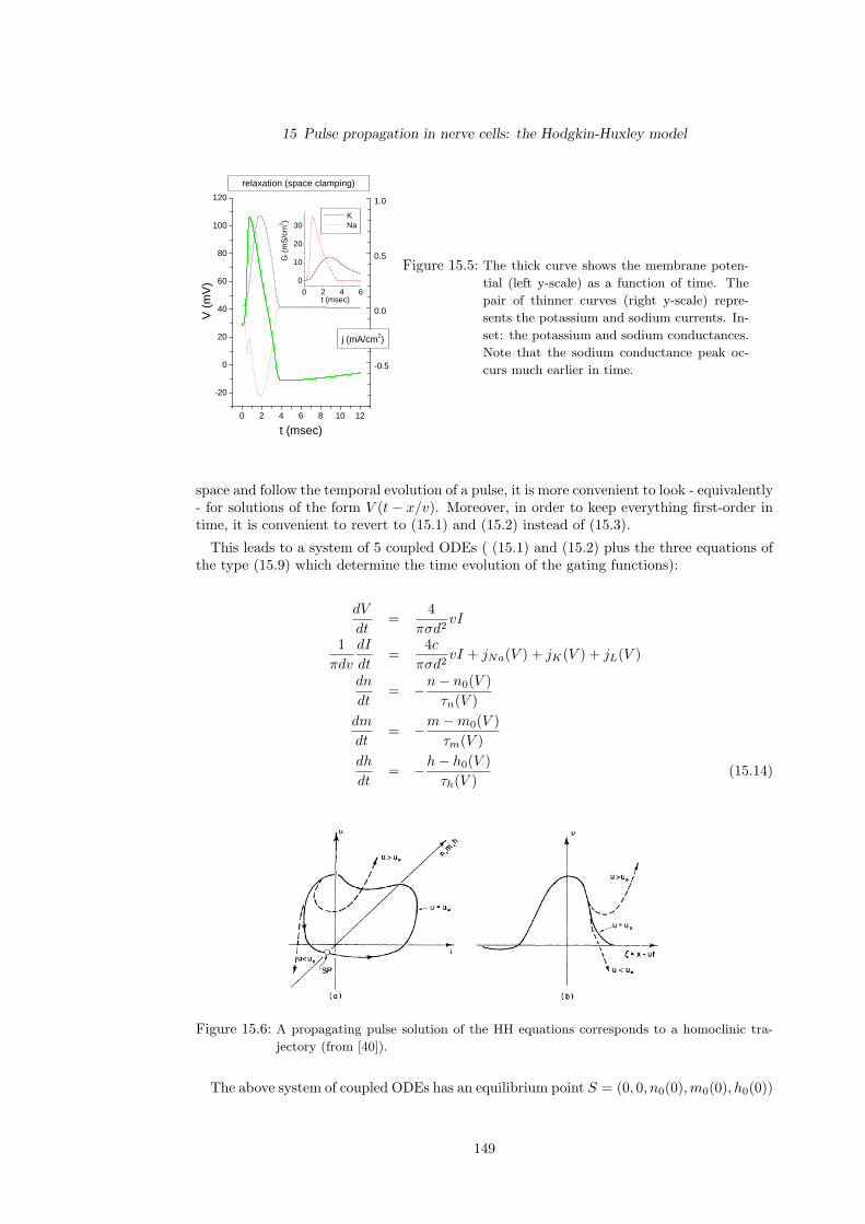
15 Pulse propagation in nerve cells: the Hodgkin-Huxley model
0 2 4 6 8 10 12
-20
0
20
40
60
80
100
120
0 2 4 6
0
10
20
30
V (
mV
)
t (msec)
relaxation (space clamping)
-0.5
0.0
0.5
1.0
j (mA/cm2)
G (
mS
/cm
2 )
t (msec)
K Na
Figure 15.5: The thick curve shows the membrane poten-
tial (left y-scale) as a function of time. The
pair of thinner curves (right y-scale) repre-
sents the potassium and sodium currents. In-
set: the potassium and sodium conductances.
Note that the sodium conductance peak oc-
curs much earlier in time.
space and follow the temporal evolution of a pulse, it is more convenient to look - equivalently- for solutions of the form V (t − x/v). Moreover, in order to keep everything first-order intime, it is convenient to revert to (15.1) and (15.2) instead of (15.3).
This leads to a system of 5 coupled ODEs ( (15.1) and (15.2) plus the three equations ofthe type (15.9) which determine the time evolution of the gating functions):
dV
dt=
4πσd2
vI
1πdv
dI
dt=
4c
πσd2vI + jNa(V ) + jK(V ) + jL(V )
dn
dt= −n− n0(V )
τn(V )dm
dt= −m−m0(V )
τm(V )dh
dt= −h− h0(V )
τh(V )(15.14)
Figure 15.6: A propagating pulse solution of the HH equations corresponds to a homoclinic tra-
jectory (from [40]).
The above system of coupled ODEs has an equilibrium point S = (0, 0, n0(0),m0(0), h0(0))
149

15 Pulse propagation in nerve cells: the Hodgkin-Huxley model
in the five-dimensional space (V, I, n, m, h). A pulse-like solution vanishes as t → ±∞. Itcorresponds to a homoclinic trajectory in the 5-dimensional space. This is shown schemati-cally in Fig. 15.6, where the three dimensions m,n, h are collapsed onto one. The trajectorystarts off at S at t = −∞; for a generic value of v it will eventually wander off to unboundedvalues of voltage and/or current. If v has the “right” value, it will return to S in the limitt → ∞. With the HH parameters, this occurs for two values of v. The first, v = 18.8
Figure 15.7: Propagating pulse solutions of the HH equations (from [40]).
m/sec, corresponds to a stable pulse with an amplitude of approximately 90 mV. The sec-ond, v = 5.7 m/sec, corresponds to an unstable pulse with a smaller amplitude (Fig. 15.7).The velocity of the stable pulse is comparable to the measured velocity, 21.2 m/sec, of thesquid’s action potential.
150
16 Localization and transport of energyin proteins: The Davydov soliton
16.1 Background. Model Hamiltonian
16.1.1 Energy storage in C=O stretching modes. Excitonic Hamiltonian
Davydov’s proposal [41] was an attempt to deal with localization and transport of energy inalpha-helical proteins. He viewed the three strands of the alpha helix as roughly independentone-dimensional chains, and assumed that energy from ATP hydrolysis (0.42 eV) could beconveniently stored in the C=O (Amide-I) stretching vibration. He then argued that if theenergy had to hop from one site to the next, following a linear (excitonic) model Hamiltonian
Hexc =∑
n
E0B
†nBn − J
(B†
n+1Bn + B†nBn+1
), (16.1)
where the Bn’s are boson operators representing the C=O stretching mode at the nthsite, and J represents the hopping parameter, it would very soon (in the order of a fewpicoseconds) be dissipated due to linear dispersion - and thus cease to be available wherereally needed, e.g. for muscular contraction.
16.1.2 Coupling to lattice vibrations. Analogy to polaron
Davydov then speculated whether the “self-trapping” effect, which had been proposed byLandau in 1933 in the context of electrons coupled to the lattice, and known in solid-statephysics as the polaron, could be applicable in the bosonic system (16.1). We have alreadydealt with a similar situation in conjugated polymers, where the coupling to the latticevibrations produces stable, propagating excitations (solitons and polarons).
Lattice vibrations are acoustic phonons represented by the Hamiltonian
Hph =∑
n
p2n
2M+
12k
∑n
(un+1 − un)2 (16.2)
where un is the displacement of the nth site from its equilibrium position, M is the massassociated with each unit of the alpha-helix, and k is a spring constant associated with thelongitudinal motion along the chain.
Coupling of the exciton modes to the lattice vibrations may occur because the energystored at a given site changes with the distance between adjacent sites, i.e. with the lengthof the hydrogen bond connecting the nth to the n + 1st site of the strand
E0 → E0 + χ(un+1 − un) .
The above coupling generates an interaction Hamiltonian of the form
Hint = χ∑
n
(un+1 − un)B†nBn . (16.3)
The total Hamiltonian is the sum of the three terms
H = Hexc + Hph + Hint . (16.4)
151

16 Localization and transport of energy in proteins: The Davydov soliton
16.2 Born-Oppenheimer dynamics
The dynamics of the coupled exciton-phonon system described by the Hamiltonian (16.4)can be considerably simplified if we make use of the Born-Oppenheimer approximation.This is not an unreasonable assumption, since acoustic vibrations are slow compared to theexcitonic modes. It allows us to treat the lattice displacements as classical variables andsimplifies the mathematical computations.
16.2.1 Quantum (excitonic) dynamics
For a given set of lattice displacements un we denote the excitonic wave function by
|Ψ >=∑
n
αn(t)B†n|0 > (16.5)
where |0 > is the bosonic vacuum state and the amplitudes αn(t) depend parametrically onthe lattice configuration un. Normalization of the quantum state demands that
∑n
|αn|2 = 1 . (16.6)
The time evolution proceeds according to the time-dependent Schrodinger equation
ih∂
∂t|Ψ >= H|Ψ > (16.7)
where H = Hexc + Hint is the quantum part of the Hamiltonian (remember, at this stageHph is just a c-number!); with the Ansatz (16.5) the Schrodinger equation (16.7) can bewritten as a set of coupled equations for the complex amplitudes
ih∂αn
∂t= E0αn + χ(un+1 − un)αn − J(αn+1 + αn−1) . (16.8)
The total energy
The expectation value of the excitonic part of the energy can be expressed in terms of theamplitudes as
< Ψ|H|Ψ >=∑
n
[E0 + χ(un+1 − un)] α∗nαn − J∑
n
α∗n(αn+1 + αn−1) . (16.9)
The total energy of a given exciton-phonon configuration un, αn is
ε =< Ψ|H|Ψ > +Hph(un) . (16.10)
The limiting case χ = 0
In the limiting case χ = 0, (16.8) reduces to
ih∂αn
∂t= E0αn − J(αn+1 + αn−1) , (16.11)
which has plane wave solutions of the form
α(q)n (t) =
1√N
ei(qx− εqh t) (16.12)
152

16 Localization and transport of energy in proteins: The Davydov soliton
with total energyεq = E0 − 2J cos qa ≡ hωq (16.13)
where the a is the lattice constant (the distance between successive sites along a single strandof the helix). These plane waves are the excitons which, according to Davydov, would exhibitdispersion over a time scale much too short to be relevant for biological energy transport.
The group velocity of excitons is given by
vg =∂ωq
∂q= 2
Ja
hsin qa . (16.14)
In the long-wavelength limit the exciton energy takes the form
εq = E0 − 2J +h2
4Ja2v2
g . (16.15)
We identify
m∗ =h2
2Ja2
as the exciton’s effective mass.
16.2.2 Lattice motion
The dynamics of the classical lattice coordinates is described by
Mun = − ∂
∂un
(Hph+ < Ψ|H|Ψ >
)
= k(un+1 + un−1 − 2un) + χ(|αn|2 − |αn−1|2) . (16.16)
16.2.3 Coupled exciton-phonon dynamics
It will prove convenient to define a new complex amplitude via
αn = φne−ih (E0−2J)t .
This allows us to rewrite (16.8) and (16.16) as
ihφn = −J(φn+1 + φn−1 − 2φn) + χ(un+1 − un)φn (16.17)
andMun = k(un+1 + un−1 − 2un) + χ(|φn|2 − |φn−1|2) (16.18)
respectively.
The general problem of coupled phonon-exciton dynamics involves the solution of theabove set of coupled ODEs.
16.3 The Davydov soliton
16.3.1 The heavy ion limit. Static Solitons
In the limit M → ∞ we may assume that ions do not move. This allows us to set theleft-hand side of (16.18) equal to zero, whereupon
un+1 − un = −χ
k|φn|2 , (16.19)
153

16 Localization and transport of energy in proteins: The Davydov soliton
which transforms (16.17) to
ihφn = −J(φn+1 + φn−1 − 2φn)− χ2
k|φn|2φn , (16.20)
and the total energy (16.10) to
∑n
E0|φn|2 − J∑
n
φ∗n(φn+1 + φn−1)− χ2
2k
∑n
|φn|4 . (16.21)
The continuum approximation
If the amplitudes vary smoothly from site to site, we can approximate the set of discretevariables φn by a continuum field φ(x). The dynamics (16.20) takes the form of thecontinuum field equation
iφτ + φxx +1σ0|φ|2φ = 0 , (16.22)
where σ0 = kJ/χ2 and I have introduced the dimensionless time τ = Jt/h.
We recognize (16.22) as the nonlinear Schrodinger (NLS) equation. In section 12.3.4 wederived a family of one soliton solutions of the form
|φ(x)| = √σ0 κ sech
κ(x− vτ)√2
with arbitrary κ and v. In the present context, since we assumed that ions do not move, vmust vanish. Furthermore, the normalization condition
∫ ∞
−∞dx |φ(x)|2 = 1
fixes the value of κ = 1/(2√
2σ0).
Form of the soliton
The exact form of the static soliton is given by
φ(x) =1√8σ0
sechx
4σ0eiτ/(16σ2
0) .
Note that the spatial extent of the soliton (in units of the lattice constant) is of the orderof 4σ0. With the standard parameter values [42] σ0 is estimated to be between 1.6 and 7.4;this appears to justify the use of the continuum approximation.
Energy considerations
The total energy of the soliton can be calculated from (16.21). The first term in (16.21)contributes E0. In the second term, we can use a Taylor expansion which produces acontribution
−2J + J
∫ ∞
−∞dx |φ′|2 = −2J +
χ4
48Jk2.
Finally, the third term produces a contribution
−χ2
2k
∫ ∞
−∞dx |φ|4 = − χ4
24Jk2.
154

16 Localization and transport of energy in proteins: The Davydov soliton
Collecting terms, I obtain the total energy of a static soliton
ε(v = 0) = E0 − 2J − χ4
48Jk2(16.23)
which lies below the excitonic band (16.13). Thus the soliton is expected to be a morestable excitation (cf. the similar argument made with the SSH kink, or the TLM polaron inconjugated polymers).
16.3.2 Moving solitons
It is straightforward to generalize the analysis of the previous subsection to the case ofmoving solitons. The system of coupled ODEs (16.17) and (16.18) can be written in thecontinuum limit as
ihφt + Jφxx − χuxφ = 0Mutt − kuxx + χ
(|φ|2)x
= 0 . (16.24)
If we look for propagating solutions of the type u(x − vt), the second equation has a firstintegral,
M(v2 − c2)ux = χ|φ|2
where Mc2 = k and I have assumed boundary conditions decaying at infinity to set theintegration constant equal to zero. The last equation, when introduced into the first of(16.24) yields
ih
Jφt + φxx +
1σ|φ|2φ = 0 (16.25)
which contains only the φ field. The parameter σ = σ0(1−v2/c2) now depends on the solitonvelocity. Again, we recognize (16.25) as the NLS equation, with a family of normalized (cf.above) solutions
φ(x, t) = ψ(x, t) eiθ
where
ψ(x, t) =1√8σ
sech(
x− vt− x0
4σ
)
θ =(
J
16hσ2+
h
4Jv2
)t +
hv
2Jx + θ0 .
The moving Davydov soliton is a coherent localized excitation which couples the quantum(excitonic) to the vibrations of the underlying lattice. Note that the above analysis is onlyvalid for positive σ. This restricts soliton velocities to v < c.
Energy of the moving soliton
Again, it is possible to calculate the total energy involved in the coupled exciton-phononsystem. The contributions can be read off (16.10) in the continuum limit:
ε(v) = E0 − 2J + J
∫dx |φ′|2 + χ
∫dx ux|φ|2 +
k
2
∫dx u2
x +M
2
∫dx u2
t
= E0 − 2J + J
∫dx
(ψ′2 + θ2
xψ2)− J
∫dx
σ|φ|4
+12J
σ0
σ
∫dx
σ|φ|4 +
12J
σ0
σ
v2
c2
∫dx
σ|φ|4
155

16 Localization and transport of energy in proteins: The Davydov soliton
≈ E0 − 2J + J
∫dx
(ψ′2 + θ2
xψ2)− J
2
∫dx
σψ4 + J
v2
c2
∫dx
σψ4
+O(v4/c4)
≈ E0 − 2J + J
(1
48σ2+
h2v2
4J2
)− J
24σ2+
J
12σ2
v2
c2
≈ E0 − 2J − χ4
48Jk2+
12m∗
sv2 +O(v4/c4) (16.26)
where the sum of the first three terms is the energy (16.23) of the static soliton and
m∗s = m∗
(1 +
Mχ4
6h2k3
)(16.27)
is the soliton’s effective mass (where I have reintroduced the lattice constant a in order torestore the proper units to m∗).
156

17 Nonlinear localization intranslationally invariant systems:discrete breathers
The existence of localized states in condensed matter systems has traditionally been associ-ated with the presence of impurities and disorder, i.e. with material behavior which breaksthe translational invariance of the perfect crystal. One of the major discoveries of the lasttwo decades in nonlinear science is that localization may also occur as a consequence ofnonlinearity in pure, translationally invariant systems of any dimensionality. A key con-tribution to this field was made by Sievers and Takeno [43] who proposed the existenceof “intrinsic localized modes” in anharmonic crystals. I will first present their argument,which is approximate and makes use of the “rotating-wave approximation”(RWA). I will thenpresent further evidence for the existence of nonlinear localized excitations - called “discretebreathers” by some authors - based on numerical calculations by Flach and coworkers [44]and give a plausibility argument which underlies the exact mathematical proof given byMacKay and Aubry [45]. For more details consult the review articles by Flach [46] andAubry [47].
17.1 The Sievers-Takeno conjecture
The starting point is the one-dimensional Hamiltonian which describes nearest-neighboratoms coupled via nonlinear springs; the anharmonicity is quartic:
H =∑
n
[p2
n
2M+
12K2(un+1 − un)2 +
12K4(un+1 − un)4
](17.1)
I try to solve the equations of motion
Mun = K2(un+1 + un−1 − 2un) + K4[(un+1 − un)3 + (un−1 − un)3] (17.2)
using the “rotating-wave approximation”, known from the theory of nuclear magnetic reso-nance. The idea is to make the Ansatz
un = α(ξne−iωt + ξ∗neiωt) (17.3)
and neglect fast oscillations which occur from terms of order e−3iωt. In the spirit of theRWA, such oscillations presumably average to zero over the time scales of interest, definedby the inverse of the frequency ω. I will further assume that the ξn’s are real, so that I keeptrack of the e−iωt terms only. Note that there are no terms of order e±2iωt. The Ansatzresults in a second order recurrence equation for the amplitudes:
2ξn − ξn+1 − ξn−1 + λ[(ξn − ξn+1)3 + (ξn − ξn−1)3
]=
ω2
Jξn (17.4)
where J = K2/M and λ = 3K4α2/K2. The value of J can be set equal to unity without
loss of generality.
157
17 Nonlinear localization in translationally invariant systems: discrete breathers
I now rewrite (17.4) as
[ω2δmn −Dmn]ξn = Vn(ξn−1, ξn, ξn+1) (17.5)
whereVn(ξn−1, ξn, ξn+1) = λ
[(ξn − ξn+1)3 + (ξn − ξn−1)3
]
the matrix elements Dmn = 2 if m = n, Dmn = −1 if m = n ± 1 and Dmn = 0 otherwisedescribe the dynamical matrix of the harmonic chain with nearest neighbor springs. Now wehave used the inverse of the matrix ω2I−D in discussing the problem of a single impurity.The matrix
(ω2 −D
)−1
mn= G(|m− n|, ω2) =
1N
∑q
e−iq(m−n)
ω2 − ω2q
, (17.6)
where the sum runs over all eigenvectors of the dynamical matrix, is known as the latticeGreen function. In the particular case we are discussing here, ω2
q = 2(1− cos q) and G hasbeen shown, for frequencies above the band, i.e, ω2 > 4, to be of the form
G(n, ω2) = (−1)|n|1ω2
g(n) , where
g(n) = (1− y)−1/2
2y
[1− 1
2y − (1− y)1/2
]|n|
∼(y
4
)|n|, (17.7)
where y = 4/ω2 and the last line gives the leading order asymptotic expansion for y ¿ 1.
Use of the lattice Green function allowed Sievers and Takeno to rewrite (17.5) as
ξm =∑
n
G(m− n, ω2)Vn(ξn−1, ξn, ξn+1) (17.8)
and exploit the rapid convergence properties of the sum in the r.h.s. of (17.8) which resultsfrom the exponential decay of the Green functions. Let us see how this works in detail:
We look for symmetric solutions of the type
ξn = (−1)|n|ηn
with η0 = 1. 1 Because of (17.4), η0 and η1 are related by the equation
1 + η1 + λ(1 + η1)3 =12ω2 =
2y
. (17.9)
In terms of the η’s, (17.8) can be written as
ηm =λ
ω2
∞∑n=−∞
g(m− n) + g(m− n + 1) (ηn + ηn+1)3 ,
which can be further symmetrized by making use of the property g(−n) = g(n), to
ηm =(
2y− 1− η1
)g(m) +
14λy
∞∑n=1
Amn(ηn + ηn+1)3 m ≥ 1 , (17.10)
whereAmn = g(m− n) + g(m− n + 1) + g(m + n) + g(m + n + 1) .
1Note that this is permissible since the scale of the amplitude has already been fixed by α in the originalAnsatz (17.3),
158

17 Nonlinear localization in translationally invariant systems: discrete breathers
Note that the m = 0 equation (which I did not write down) is not really independent, since itmust be equivalent to (17.9). The system of coupled nonlinear equations (17.9) and (17.10)can in principle be solved numerically to yield the amplitudes and the eigenfrequency. Thenumerical procedure would presumably converge fast, due to the exponential decay of theAmn’s. In practice, only a few terms are expected to contribute to the sum.
However, one can already make some statements using the asymptotic properties of theGreen functions in the limit y ¿ 1.
To leading order in y, the m = 1 equation (17.10) gives
η1 ∼ 12
which can be used in (17.9) to compute the eigenvalue. The result
y =4ω2
=1
34 + 27
16λ
gives a consistent value of y À 1 if λ À 4/27. For sufficiently strong nonlinearities, onetherefore has
ω2 ∼ 3 +274
λ. (17.11)
17.2 Numerical evidence of localization
An illuminating picture of nonlinear localization as “local integrability” was obtained throughnumerical simulations by Flach and coworkers [44]. I summarize some of their findings.
The starting point is the one-dimensional Hamiltonian
H =∑
n
[p2
n
2+
12C(un+1 − un)2 + V (un)
](17.12)
with a moderately weak harmonic interparticle coupling strength C = 0.1 and a nonlinearon-site potential
V (u) = u2 − u3 +14u4 .
The equations of motion
un = C(un+1 + un−1 − 2un)− V ′(un) i = 0,±1, · · · ±N/2 (17.13)
were numerically integrated for a lattice of N = 3000 sites, subject to periodic boundaryconditions. The initial condition was spatially localized, i.e. all particles started at rest,un = 0 ∀n and all but one of them (at the n = 0 site) were at the equilibrium positionscorresponding to the absolute minimum of (17.12).
A measure of the energy density at the lth site is given by
el =12u2
l + V (ul) +C
4[(ul+1 − ul)2 + (ul − ul−1)2
]. (17.14)
Note that the sum over all el’s is by definition a conserved quantity, the total energy.
159

17 Nonlinear localization in translationally invariant systems: discrete breathers
Figure 17.1: The temporal evolution of e(5). The solid line shows the total energy. In the inset,
the energy distribution around the central site, measured for 1000 < t < 1150 (from
[44] ).
17.2.1 Diagnostics of energy localization
An empirical diagnosis of localization can be made in terms of the quantities
e(2m+1) =m∑−m
el , (17.15)
which provide a measure of the energy residing in the first 2m + 1 central sites. If these canbe shown to remain constant over long periods of time, one may reasonably conjecture thepresence of a localized oscillation which keeps the energy around the central sites. Fig. 17.1describes the temporal evolution of e(5). There is some radiation, amounting to less than1% of the total energy, which occurs during the first few hundred time units. After thesetransients decay however, the energy stays remarkably constant.
17.2.2 Internal dynamics
It is possible to obtain additional information about the internal dynamics of the localizedoscillation by looking at the Fourier spectra of the few central sites. The numerical resultsare shown in Fig. 17.2. The spectra of the central site, l = 0, shows a dominant peak atω1 = 0.822. The spectra of the sites l = ±1 show a dominant peak at ω2 = 1.34. Allother peaks of both spectra can be obtained as sums or differences of these two fundamentalfrequencies. This remarkable result suggests that we are, in effect, dealing with a system oftwo degrees of freedom.
This suggestion can be tested in some more detail by looking at the reduced dynamicalsystem with two degrees of freedom
u0 = −V ′(u0) + 2C(u1 − u0) (17.16)u1 = −V ′(u1) + C(u0 − 2u1) (17.17)
which is obtained from the full dynamics (17.13) by assuming all particles with |l| > 1 toremain at rest, and exploiting the symmetry u−1 = u1.
160

17 Nonlinear localization in translationally invariant systems: discrete breathers
Figure 17.2: Fourier spectra of u0(t > 1000). Inset: spectra of u1. All peak frequencies are either
sums or differences of the two fundamental frequencies. (From [44] ).
Fig. 17.3 shows a Poincare cut of this reduced dynamical system. Note the presenceof regular motion (tori) embedded in a sea of chaos. Flach and coworkers [44] made, andtested, the following remarkable conjecture: If the frequencies of a torus lie outside thephonon band of the linearized version of (17.13), the torus should correspond to a localizedoscillation of the full system. Indeed, a choice of initial condition from the islands 1 or 2generates a localized oscillation in the full system (17.13). A choice from island 3, or froma chaotic trajectory, generates a nonlocalized pattern. This is shown in detail in Fig. 17.4.
17.3 Towards exact discrete breathers
Consider a Hamiltonian of the type (17.12) which describes a system of N weakly couplednonlinear oscillators. The spatial dimensionality is not important for the arguments whichfollow. Let the state of the system be described at any given time by the 2N -dimensionalvector
~X = x1, · · ·xN ; p1 · · · pN .
At zero coupling strength it is possible to excite a single oscillator at the lth site and leaveall other particles at rest. The motion of the system will be periodic, with a given period
161

17 Nonlinear localization in translationally invariant systems: discrete breathers
Figure 17.3: Poincare cut of the reduced dynamical system at E = 0.58. (From [44] ).
Figure 17.4: Temporal evolution of e(5) for a variety of initial conditions chosen according to their
properties in the reduced system. Localization occurs for 4 initial conditions chosen
from fixed points in islands 1 and 2 in Fig. 17.3, the larger torus in island 1, and
the torus in island 2 (solid lines). Initial conditions from the torus in island 3 (long-
dashed line), or from a chaotic trajectory (dashed-dotted line) lead to decaying e(5).
The upper short-dashed line shows the total energy of all simulations. (From [44] ).
T . I denote this by~X0(t) = ~X0(t + T ) .
Now consider what happens when a weak coupling is turned on. The time evolution of thesystem over a time T , generated by the full Hamiltonian, transforms any initial state vector~X(0) (denoted from now on as ~X for simplicity) to ~X(T ). Let
~F [ ~X] = ~X(T )− ~X
formally denote the operator which performs this time evolution.
Periodic orbits of the interacting system correspond to roots of the 2N coupled equations
~F [ ~X] = 0 . (17.18)
Since a weak coupling was assumed, it is not unreasonable to expect the initial condition~X0 of the decoupled system - which is known to lead to a periodic orbit there - to lie nearthe root of (17.18). We could then use this a starting point for a Newton-like iteration
162

17 Nonlinear localization in translationally invariant systems: discrete breathers
procedure2, i.e. proceed to construct a next iterate ~X1 near the original guess ~X0 bydemanding that
~F [ ~X1] = ~F [ ~X0] + M0 ·(
~X1 − ~X0)
= 0
where the elements of the 2N × 2N matrix M0 are given by
M0mn =
∂Fm
∂X0n
=∂Xm(T )
∂Xn
∣∣∣∣~X= ~X0
− δmn . (17.19)
This is equivalent to demanding
~X1 = ~X0 − [M0
]−1 ~F [ ~X0]
which can be continued as~Xj+1 = ~Xj − [
Mj]−1 ~F [ ~Xj ] (17.20)
until convergence to the “true” discrete breather is achieved. This can also be a practicalmethod to construct exact breather solutions to machine numerical accuracy. It is successful,provided that (a) the matrix M is invertible, and (b) that the breather frequency ωb = 2π/Thas no resonances of the type
nωb = ωq (17.21)
with the phonon band. Note that this generally allows breathers with frequencies above thephonon bands without any restrictions, but may impose severe limits to breathers whosefrequencies lie below a phonon band. For example, in the case of the Hamiltonian (17.12),breather frequencies must lie outside the frequency ranges
1 < nωb < (1 + 4C)1/2 n = 1, 2, 3, · · ·(cf. Fig. 17.5).
Figure 17.5: Forbidden frequency bands (in color) for DBs
in the case of the Hamiltonian (17.12). The
dotted line represents the linear phonon dis-
persion curve. Note that the bands with n > 5
merge, leaving no frequency region allowed for
DBs.
0 1 2 30.0
0.5
1.0
1.5
Fre
quen
cy
k
Details of the existence proof for discrete breathers can be found in Ref. [45].2The Newton procedure for locating roots of f(x) = 0 starts from a “guess” x0 with f(x0) not too far from
zero, and iterates successively,
xj+1 = xj −(
df
dx
)−1
x=xj
f(xj) .
Provided that the guess does not lead away from the true root, the procedure is rapidly (quadratically)convergent.
163

A Impurities, disorder and localization
In the following, I will try to illustrate, with the help of characteristic examples, how dis-order can lead to localization of eigenstates. The point is not to present exact criteria forlocalization; this would be beyond the scope of these lectures. Nonetheless, the simple ex-amples treated should make clear that (i) an isolated eigenstate, i.e. one which is outsidethe phonon (or electron, depending on the problem) bands, will tend to be localized, and(ii) the introduction of disorder will transform most eigenstates from extended to localizedones. In other words, these examples serve to illustrate the obvious, i.e. that breaking trans-lational invariance will introduce some degree of localization; at the same time, they remindus the basic condition for the existence of isolated localized states, i.e. that the frequency ofoscillation should lie outside any bands.
A.1 Definitions
A.1.1 Electrons
Consider a one-dimensional tight-binding electron Hamiltonian
H =∑
n
εnc†ncn − tn,n+1(c
†n+1cn + h.c)
(A.1)
where the on-site energies εn and the hopping amplitudes tn,n+1 may depend on the latticesite.
We look for eigenstates of (A.1)
H|Ψ >= E|Ψ >
in the subspace of one-electron states:
|Ψ >=∑
n
ψnc†n|0 > (A.2)
The amplitudes ψn must then satisfy the difference eigenvalue equation
−tn,n−1ψn−1 − tn,n+1ψn+1 + εnψn = Eψn . (A.3)
Limiting cases are
• the translationally invariant case tn = t0, εn = ε0∀n. The eigenstates are plane waves
ψ(q)n =
1√N
eiqn
with the corresponding eigenvalues
Eq = ε0 − 2t0 + 2t0(1− cos q)
.
• diagonal disorder tn,n+1 = t0 ∀n .
• off-diagonal disorder εn = ε0 ∀n .
• a single impurity of either type, e.g εn = ε0 if n 6= α, εα = ε′
.
164
A Impurities, disorder and localization
A.1.2 Phonons
Lattice vibrations in disordered harmonic lattices are described by the same mathematics.Consider the Hamiltonian
H =∑
n
p2n
2µn+
12
∑n
kn,n+1(xn+1 − xn)2 +12
∑n
vnx2n (A.4)
where, in general, masses and spring constants depend on the lattice site; note that I haveadded a harmonic on-site term. The coefficients vn will of course vanish in the usual harmonicchain with nearest-neighbor springs only.
The classical equations of motion corresponding to (A.4) are
µnxn = kn,n+1xn+1 + kn,n−1xn−1 − (kn,n+1 + kn,n−1 + vn)xn ; (A.5)
if we look for normal modes of (A.5) with the Ansatz
xn(t) =1õn
ψneiωt , (A.6)
the amplitudes must satisfy the difference eigenvalue equation
−tn,n−1ψn−1 − tn,n+1ψn+1 + εnψn = ω2ψn , (A.7)
where tn,n+1 = (µnµn+1)−1/2kn,n+1 and εn = (kn,n+1 + kn,n−1 + vn)/µn.
Limiting cases of interest are
• the translationally invariant case: kn,n+1 = k, µn = µ, vn = v ∀n. The eigenstatesare plane waves
ψ(q)n =
1√N
eiqn
with the corresponding eigenvalues
ω2q =
1µ
[v + 2k(1− cos q)] .
• mass disorder: kn,n+1 = k ∀n , µn random.
• spring disorder: µn = µ ∀n , kn random.
• a single impurity of either type, e.g µn = µ if n 6= α, µα = µ′
(isotopic massimpurity).
• on-site single impurity (corresponds to diagonal disorder at a single site): kn,n+1 =k, µn = µ, ∀n, vn = v if n 6= α, vα = v
′.
Note that in the most general case considered here, one has to diagonalize a tridiagonal N×Nreal symmetric matrix. This can be done with very efficient numerical techniques[48].
A.2 A single impurity
A.2.1 An exact result
The case of a lattice impurity which modifies only a single diagonal element of the dynamicalmatrix has been treated exactly by M. Lax [49] and provides substantial insight. I presentthe original derivation and elaborate on the special case of one dimension.
165
A Impurities, disorder and localization
Consider the more general problem where one knows the spectrum of a given dynamicalmatrix D,
Dij ej(p) = λ(p) ei(p) i = 1, · · ·N (A.8)
and is interested in the spectrum of a modified matrix D + B, where the modification B isof reduced dimensionality, i.e.
Brs 6= 0 only if r, s = 1, · · · k; k ¿ N.
Let ~ψ be an eigenvector of the modified matrix, corresponding to an eigenvalue Λ:
(Dij + Bij)ψj = Λψi
It follows that
(Λδij −Dij)ψi = Bijψj
ψi = (ΛI−D)−1ij Bjkψk
= (ΛI−D)−1ir Brsψs
=∑
p
e∗i (p) er(p)Λ− λ(p)
Brsψs (A.9)
where in the last line I have used the standard representation of the inverse of D in termsof its spectrum.
Let me now consider the special case where k = 1, i.e.
Bij = bδiαδjα
(on-site lattice impurity at the site α, cf. above). The condition (A.9) becomes
ψi = b∑
p
e∗i (p) eα(p)Λ− λ(p)
ψα . (A.10)
If the unperturbed matrix describes a translationally invariant system, the eigenvectors willbe plane waves, i.e.
ej(p) =1√N
ei~p·~Rj (A.11)
where ~p is the wavevector corresponding to the eigenvalue index p. (Note that up to nowthere are no restrictions to dimensionality.) Using the plane-wave form of the eigenvectors,I rewrite (A.10) as
ψi =b
N
∑p
e−i~p(~Ri−~Rα)
Λ− λ(p)ψα . (A.12)
which, for i = α, becomes1N
∑p
1Λ− λ(p)
=1b
. (A.13)
Locating states outside the band
Eq. (A.13) is an Nth order algebraic equation. It is straightforward to see that a rootmust exist between any pair of successive eigenvalues λ(p) < Λ < λ(p + 1). This providesN − 1 roots. The Nth root will therefore lie outside the band. In this case however, one
166
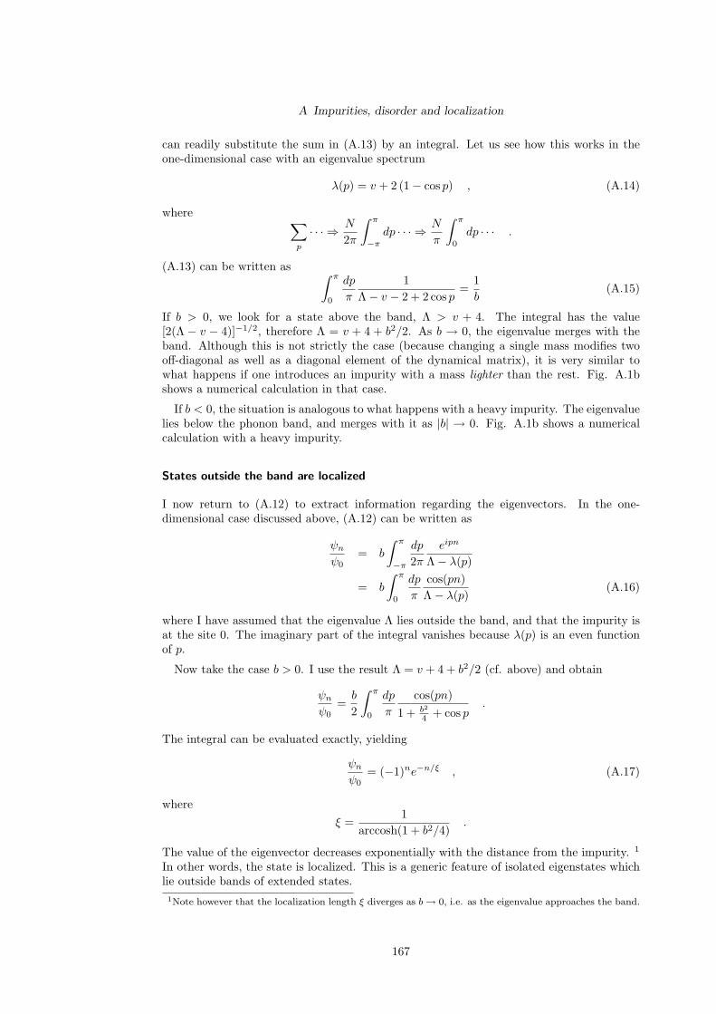
A Impurities, disorder and localization
can readily substitute the sum in (A.13) by an integral. Let us see how this works in theone-dimensional case with an eigenvalue spectrum
λ(p) = v + 2 (1− cos p) , (A.14)
where ∑p
· · · ⇒ N
2π
∫ π
−π
dp · · · ⇒ N
π
∫ π
0
dp · · · .
(A.13) can be written as ∫ π
0
dp
π
1Λ− v − 2 + 2 cos p
=1b
(A.15)
If b > 0, we look for a state above the band, Λ > v + 4. The integral has the value[2(Λ − v − 4)]−1/2, therefore Λ = v + 4 + b2/2. As b → 0, the eigenvalue merges with theband. Although this is not strictly the case (because changing a single mass modifies twooff-diagonal as well as a diagonal element of the dynamical matrix), it is very similar towhat happens if one introduces an impurity with a mass lighter than the rest. Fig. A.1bshows a numerical calculation in that case.
If b < 0, the situation is analogous to what happens with a heavy impurity. The eigenvaluelies below the phonon band, and merges with it as |b| → 0. Fig. A.1b shows a numericalcalculation with a heavy impurity.
States outside the band are localized
I now return to (A.12) to extract information regarding the eigenvectors. In the one-dimensional case discussed above, (A.12) can be written as
ψn
ψ0= b
∫ π
−π
dp
2π
eipn
Λ− λ(p)
= b
∫ π
0
dp
π
cos(pn)Λ− λ(p)
(A.16)
where I have assumed that the eigenvalue Λ lies outside the band, and that the impurity isat the site 0. The imaginary part of the integral vanishes because λ(p) is an even functionof p.
Now take the case b > 0. I use the result Λ = v + 4 + b2/2 (cf. above) and obtain
ψn
ψ0=
b
2
∫ π
0
dp
π
cos(pn)1 + b2
4 + cos p.
The integral can be evaluated exactly, yielding
ψn
ψ0= (−1)ne−n/ξ , (A.17)
whereξ =
1arccosh(1 + b2/4)
.
The value of the eigenvector decreases exponentially with the distance from the impurity. 1
In other words, the state is localized. This is a generic feature of isolated eigenstates whichlie outside bands of extended states.1Note however that the localization length ξ diverges as b → 0, i.e. as the eigenvalue approaches the band.
167
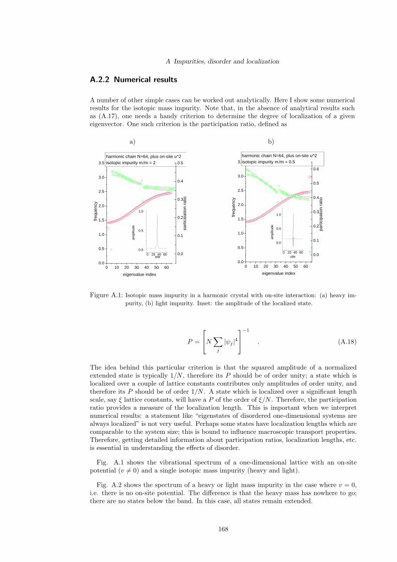
A Impurities, disorder and localization
A.2.2 Numerical results
A number of other simple cases can be worked out analytically. Here I show some numericalresults for the isotopic mass impurity. Note that, in the absence of analytical results suchas (A.17), one needs a handy criterion to determine the degree of localization of a giveneigenvector. One such criterion is the participation ratio, defined as
a) b)
0 10 20 30 40 50 600.0
0.5
1.0
1.5
2.0
2.5
3.0
3.5
0 20 40 600.0
0.5
1.0
part
icip
atio
n ra
tio
freq
uenc
y
eigenvalue index
harmonic chain N=64, plus on-site u^2isotopic impurity m'/m = 2
0.0
0.1
0.2
0.3
0.4
0.5
ampl
itude
site
0 10 20 30 40 50 600.0
0.5
1.0
1.5
2.0
2.5
3.0
3.5
0 20 40 60
0.0
0.5
1.0
part
icip
atio
n ra
tio
freq
uenc
y
eigenvalue index
harmonic chain N=64, plus on-site u^2isotopic impurity m'/m = 0.5
0.0
0.1
0.2
0.3
0.4
0.5
0.6
ampl
itude
site
Figure A.1: Isotopic mass impurity in a harmonic crystal with on-site interaction: (a) heavy im-
purity, (b) light impurity. Inset: the amplitude of the localized state.
P =
N
∑
j
|ψj |4−1
. (A.18)
The idea behind this particular criterion is that the squared amplitude of a normalizedextended state is typically 1/N , therefore its P should be of order unity; a state which islocalized over a couple of lattice constants contributes only amplitudes of order unity, andtherefore its P should be of order 1/N . A state which is localized over a significant lengthscale, say ξ lattice constants, will have a P of the order of ξ/N . Therefore, the participationratio provides a measure of the localization length. This is important when we interpretnumerical results: a statement like “eigenstates of disordered one-dimensional systems arealways localized” is not very useful. Perhaps some states have localization lengths which arecomparable to the system size; this is bound to influence macroscopic transport properties.Therefore, getting detailed information about participation ratios, localization lengths, etc.is essential in understanding the effects of disorder.
Fig. A.1 shows the vibrational spectrum of a one-dimensional lattice with an on-sitepotential (v 6= 0) and a single isotopic mass impurity (heavy and light).
Fig. A.2 shows the spectrum of a heavy or light mass impurity in the case where v = 0,i.e. there is no on-site potential. The difference is that the heavy mass has nowhere to go;there are no states below the band. In this case, all states remain extended.
168

A Impurities, disorder and localization
a) b)
0 10 20 30 40 50 600.0
0.5
1.0
1.5
2.0
2.5
0 20 40 60
-0.2
0.0
0.2
0.4
part
icip
atio
n ra
tio
freq
uenc
y
eigenvalue index
harmonic chain N=64isotopic impurity m'/m = 5inset: "most" localized EV
0.0
0.2
0.4
0.6
ampl
itude
site
0 10 20 30 40 50 600.0
0.5
1.0
1.5
2.0
2.5
0 20 40 60-0.5
0.0
0.5
1.0
part
icip
atio
n ra
tio
freq
uenc
y
eigenvalue index
harmonic chain N=64isotopic impurity m'/m = 0.5
0.0
0.1
0.2
0.3
0.4
0.5
0.6
0.7
ampl
itude
site
Figure A.2: as in previous figure, no on-site term. The light mass impurity does not generate a
localized state, because there are no states below the phonon band. Inset: right: the
localized state, left: the “most” localized state (the one with the lowest participation
ratio) is still an extended state.
A.3 Disorder
Here I show numerical results obtained for a selection of random distribution of potentialparameters.
A.3.1 Electrons in disordered one-dimensional media
Figs. A.3 and A.4 show one-electron spectra of disordered one-dimensional system (A.3).The disorder is of the diagonal type, i.e. the tn,n+1 = 1 and εn = 2 + Wrn, where rn is arandom number between −1/2 and 1/2, and and the strength of the disorder increases fromW = 1 to W = 4. Fig. A.5a is a histogram of the density of states for W = 2; Fig. A.5bis a histogram of participation ratios for W = 1, 2, 4. Note the drastic increase of localizedstates which occurs at W = 4.
A.3.2 Vibrational spectra of one-dimensional disordered lattices
Figs. A.6 and A.7 show the effect of mass disorder in the one-dimensional harmonic lattice.The masses are generated according to µi = eWri , where ri is a random number between−0.5 and 0.5 and the strength of the disorder is W = 4. Note the proliferation of localizedstates. Only the very lowest frequencies correspond to extended states.
169

A Impurities, disorder and localization
a) b)
0 20 40 60 80 100 120 140-1.0
-0.5
0.0
0.5
1.0
1.5
2.0
2.5
3.0
3.5
4.0
4.5
5.0
0 50 100-0.15
-0.10
-0.05
0.00
0.05
0.10
0.15
part
icip
atio
n ra
tiofreq
uenc
y
eigenvalue index
Schr discr,N=128, plus on-site u^2no disorder
0.50
0.55
0.60
0.65
0.70
0.75
0.80
ampl
itude
site
0 20 40 60 80 100 120 140-1.0
-0.5
0.0
0.5
1.0
1.5
2.0
2.5
3.0
3.5
4.0
4.5
5.0
0 50 100
0.0
0.5
part
icip
atio
n ra
tio
freq
uenc
y
eigenvalue index
0.0
0.1
0.2
0.3
ampl
itude
site
Figure A.3: Spectrum of one-electron states : (a) reference (no disorder), (b) diagonal disorder
W = 1.
a) b)
0 20 40 60 80 100 120 140-4
-2
0
2
4
6
8
80 100 120
0.0
0.5
part
icip
atio
n ra
tio
freq
uenc
y
eigenvalue index
0.00
0.02
0.04
0.06
0.08
0.10
0.12
0.14
0.16
0.18
0.20
0.22
0.24
0.26
0.28
0.30
ampl
itude
site
0 20 40 60 80 100 120 140-4
-2
0
2
4
6
8
90 95 100 105
0.0
0.5
1.0pa
rtic
ipat
ion
ratio
freq
uenc
y
eigenvalue index
0.00
0.02
0.04
0.06
0.08
ampl
itude
site
Figure A.4: Spectrum of one-electron states : (a) as in previous, W = 2, (b) W = 4.
170

A Impurities, disorder and localization
a) b)
-4 -2 0 2 4 6 80
2
4
6
8
10
12
14
16
18
num
ber
of s
tate
s
energy
W=2
0.0 0.1 0.2 0.30
20
40
60
80
100
num
ber
of s
tate
s
inv. partic.
W 1 2 4
Figure A.5: Spectrum of one-electron states : (a) Density of states W = 2, (b) Histogram of
participation ratios, W = 1, 2, 4.
a) b)
0 500 10000.0
0.5
1.0
1.5
2.0
2.5
3.0
3.5
4.0
4.5
5.0
410 420-0.5
0.0
0.5
1.0
1.5
part
icip
atio
n ra
tiofreq
uenc
y
eigenvalue index
harm latticemass disorder 4
0.0
0.1
0.2
0.3
0.4
ampl
itude
site
0 1 2 3 4 50
50
100
Num
ber
of s
tate
s
frequency
B
Figure A.6: Mass disorder in the harmonic lattice W=4 : (a) spectrum, and degree of localization,
(b) Frequency Histogram.
171

A Impurities, disorder and localization
a) b)
0.0 0.1 0.2 0.30
200
400
600
800
Num
ber
of s
tate
s
Inverse participation ratio
C
0.01 0.1 1 10
1E-3
0.01
0.1
Inv
part
icip
atio
n ra
tio
frequency
Figure A.7: Mass disorder in the harmonic lattice W=4 : (a) The vast majority of states are
localized. (b) A detailed view of localization vs. frequency: Localization lengths can
become significantly large at low frequencies. There is a low frequency regime where
theory predicts that the localization length grows as the inverse square of the frequency
(dotted line). At the very lowest frequencies this theoretically predicted localization
length is limited by finite size effects.
172

Bibliography
[1] P.Chr. Hemmer, L.C. Maximon and H. Wergeland, Phys. Rev. 111, 689 (1958).
[2] E. Fermi, J. Pasta and S. Ulam, Los Alamos report LA -1940 (1955), published inCollected papers of Enrico Fermi, E. Segre (Ed.), University of Chicago Press (1965).
[3] C.Y. Lin, S.N. Cho, C.G. Goedde and S. Lichter, Phys. Rev. Lett. 82, 259 (1999).
[4] J. Ford, Phys. Reports 213, 271 (1992).
[5] John Scott Russell, Report on Waves (Report of the fourteenth meeting of the BritishAssociation for the Advancement of Science, York, September 1844 (London 1845), pp311-390, Plates XLVII-LVII).
[6] D.J. Korteweg and G. deVries, Phil. Mag. [5], 39, 422 (1895).
[7] I.M. Gel’fand, B.M. Levitan, Amer. Math. Soc. Transl. 1, 253 (1955).
[8] Marchenko
[9] L.D. Faddeev, J. Math. Phys. 4, 72 (1963).
[10] A.C. Scott, F.V.F. Chu and D. McLaughlin, Proc. IEEE 61, 1473 (1973).
[11] M. Toda, Phys. Repts. (1975); Theory of nonlinear lattices, Springer (1988)
[12] M. Henon and C. Heiles, Astron. J. 69, 73 (1964).
[13] L.E. Reichl and W.M. Zheng, Phys. Rev. A 29, 2186 (1984).
[14] S.J. Shenker and L.P. Kadanoff, J. Stat. Phys. 27, 631 (1982).
[15] J.M. Greene, J. Math. Phys. 20, 1183 (1979).
[16] J.D. Meiss, Rev. Mod. Phys. 64, 795 (1992).
[17] M.H. Jensen, P. Bak and T. Bohr, Phys. Rev. A 30, 1960 (1984).
[18] E. Ott, Chaos in Dynamical Systems, Cambridge (2002).
[19] M. Tabor, Chaos and integrability in nonlinear dynamics, Wiley (1989).
[20] J. Frenkel and T. Kontorova, Phys. Z. Sowjet. 13, 1 (1938).
[21] F.C. Frank and J.H. van der Merwe, Proc. Roy. Soc. Lond. A198, 205 (1949).
[22] P.M. Chaikin and T.C. Lubensky, Principles of condensed matter physics, CambridgeUniversity Press (1995).
[23] S. Aubry in Solitons and Condensed Matter Physics (Eds. A.R. Bishop and T. Schnei-der), p. 264, Springer (1978); S. Aubry and P.Y. Le Daeron, Physica D 8, 381 (1983).
[24] M. Peyrard and S. Aubry, J. Phys. C 16, 1593 (1983).
173
Bibliography
[25] W. Chou and R.B. Griffiths, Phys. Rev. B 34, 6219 (1986).
[26] O.V. Zhirov, G. Casati and D.L. Shepelyansky, Phys. Rev. E 65, 026220 (2002).
[27] H.J. Mikeska and M. Steiner, Adv. Phys. 40, 191 (1991).
[28] J.P. Boucher, L.P. Regnault, J. Rossat-Mignaud, Y. Henry, J. Bouillot, W.G. Stirlingand F. Mezei, Physica B, 120, 141 (1983).
[29] A.J. Heeger, Rev. Mod. Phys. 73, 681 (2001).
[30] A.J. Heeger, S. Kivelson, J.R. Schrieffer and W.P. Su, Rev. Mod. Phys. 60, 781 (1988).
[31] W.P. Su, J.R. Schrieffer and A.J. Heeger, Phys. Rev. Lett. 42, 1698 (1979).
[32] H. Takayama, Y.R. Lin-Liu and K. Maki, Phys. Rev. B 21, 2388 (1980).
[33] L. Pitaevskii and S. Stringari, Bose-Einstein Condensation, Oxford University Press(2003).
[34] A.J. Leggett, Rev. Mod. Phys. 73, 307 (2001).
[35] S. Burger, K. Bongs, S. Dettmer, W. Ertmer, K. Sengstock, A. Sanpera, G. V. Shlyap-nikov and M. Lewenstein, Phys. Rev. Lett. 83, 5198 (1999).
[36] R.B. Inman and R.L. Baldwin, J. Mol. Biol. 8, 452 (1964).
[37] M. Peyrard and A.R. Bishop, Phys. Rev. Lett. 62, 2755 (1989).
[38] L.D. Landau and E.M. Lifshitz, Nonrelativistic Quantum Mechanics, Pergamon Press(1977).
[39] N. Theodorakopoulos, M. Peyrard and R.S. MacKay, Phys. Rev. Lett. 93, 258101(2004).
[40] A.C. Scott, Rev. Mod. Phys. 47, 487 (1975).
[41] A.S. Davydov, J. Theor. Biol. 38, 559 (1973).
[42] A.C. Scott, Phys. Reports 217, 1 (1992).
[43] A. Sievers and S. Takeno, Phys. Rev. Lett. 61, 970 (1999).
[44] S. Flach, C.R. Willis and E. Olbrich, Phys. Rev. E 49, 836 (1994).
[45] R.S. MacKay and S. Aubry, Nonlinearity 7, 1623 (1994).
[46] S. Flach and C.R. Willis, Phys. Reports 295, 181 (1998).
[47] S. Aubry, Physica D 216, 1 (2006).
[48] W.H. Press, B.P. Flannery, S.A. Teukolsky and W.T. Vetterling, Numerical Recipes inFORTRAN: The Art of Scientific Computing, Cambridge University Press (1992).
[49] M. Lax, Phys. Rev. 94, 1391 (1954).
174


![Chaos, Solitons and Fractals - Brown University · 328 F. Song, G.E. Karniadakis / Chaos, Solitons and Fractals 102 (2017) 327–332 incompressible flows [17,18] and for the fractional](https://static.fdocuments.net/doc/165x107/5f703e3061762a11ee05c214/chaos-solitons-and-fractals-brown-university-328-f-song-ge-karniadakis-.jpg)


