Nonlinear Modelling of Chemical Kinetics -Tuszynski
62
NONLINEAR MODELLING OF CHEMICAL KINETICS FOR THE ACID MINE DRAINAGE PROBLEMANDRELATED PHYSICAL TOPICS MEND Project 1.51.2 This work was done on behalf of MEND and sponsored by Environment Canada October 1993
-
Upload
andrequiroz2008 -
Category
Documents
-
view
223 -
download
2
Transcript of Nonlinear Modelling of Chemical Kinetics -Tuszynski

NONLINEAR MODELLING OF CHEMICAL KINETICS FOR THE ACID MINE DRAINAGE
PROBLEMANDRELATED PHYSICAL TOPICS
MEND Project 1.51.2
This work was done on behalf of MEND and sponsored by Environment Canada
October 1993

MEND PARTICIPANTS NEDEM
Association mini&e du Quebec
Atomic Energy Control Board BHP Minerals Limited
British Columbia Ministry of Energy, Mines and Petroleum Resources Brunswick Mining & Smelting
Cambior Inc.
Canada Centre for Mineral and Energy Technology Cape Breton Development Corporation
Centre de recherches minerales Cominco Limited
Den&n Mines Limited Echo Bay Mines Limited
Environment Canada Falconbridge Limited Fisheries and Oceans
Homestake Canada
Hudson Bay Mining and Smelting Company Limited INCO Limited
Indian and Northern Affairs Canada Lac Minerals
Les Mines Selbaie Les Ressources Aur Inc.
Manitoba Energy and Mines Ministere de 1’Energie et des Ressources du Qut%ec
Ministere de 1’Environnement et de la Faune du Qut%ec Minnova Ltd.
N.B. Coal
Natural Resources Canada
New Brunswick Department of Natural Resources and Energy Newfoundland and Labrador Department of Mines and Energy
Noranda Minerals Inc. Nova Scotia Department of Natural Resources
Ontario Ministry of Environment Ontario Ministry of Northern Development and Mines
Placer Dome Inc. Rio Algom Limited
Saskatchewan Environment and Resource Management Teck Corporation
The Mining Association of British Columbia The Mining Association of Canada
The Mining Association of Ontario Westmin Resources Limited
Associate P2wticipant.S Assods
Australian Nuclear Science & Technology Organization Ecole Polytechnique
European Commission
Geological Survey of Canada National Mine Land Reclamation Centre Norwegian Pollution Control Authority
Swedish National Environmental Protection Board
Laurentian University United States Bureau of Mines University of British Columbia
University of Waterloo University of Western Ontario
US Geological Survey
1994

NONLINEAR MODELLING OF CHEMICAL KINETICS
FOR THE ACID MINE DRAINAGE PROBLEM
AND RELATED PHYSICAL TOPICS
FINAL REPORT
Submitted to the
British Columbia Acid Mine
Drainage Task Force
bY
J.A. Tuszyriski’, M.L.A. Nip and D. Sept*
Department of Physics
University of Alberta
Edmonton, Alberta, T6G 251
* present address:
Institut fiir Theoretische Physik I
Heinrich-Heine Universit%t Diisseldorf
D-40225 Diisseldorf

Contents
S.ummary 2
1 Introduct ion 3
2 Nonlinear Chemical Kinetics 5 2.1 Homogeneous Media . . . . . . . . . . . . . . . . . . . . . . . . . . . . . . 5 2.2 Reactions in Porous Media . . . . . . . . . . . . . . . . . . . . . . . . . . . 9
3 The Chemical Processes in AMD 10 3.1 Introductory Comments ............................ 10 3.2 Acid Generation ................................. 10
3.3 Acid Neutralization ............................... 13
4 Modelling and Its Results 15 4.1 Acid Production (Homogeneous Medium) ...... ; ............ 15 4.2 Acid Production (Porous Medium) ...................... 18 4.3 Acid Neutralization Reactions ......................... 19
5 Discussion and F’uture Outlook 32 5.1 Summary and Conclusion ........................... 32
5.2 Future Outlook ................................. 34 5.3 Rocks: characterization and flow properties .................. 36
An Introductory Overview of Nonlinear Phenomena 42 A: Chaotic Behavior ................................ 42 B: Coupled Systems and Limit Cycles ...................... 43 C: Strange Attractors and Prediction Limitations ................ 46 D: F’ractals ..................................... 48 E: Percolation Process ............................... 50
F: Pattern Formation ............................... 51
Summary
The problem of Acid Mine Drainage (AMD) poses a significant environmental danger in British Columbia and other parts of the world involved in mining activities. Oxygena- tion reactions responsible for the chemical generation of acidity have been, by and large, identified. Thus far rather simplified modelling techniques have been used in the analysis of these complex reactions that possess feedback loops characteristic of chemical chaos systems. Our primary objective was to provide an in-depth study of the basic reactions in the AMD problem; to model the associated chemical kinetics and draw conclusions regarding the predictability of these nonlinear processes.
Having derived the constituent differential equations under several sets of conditions we have applied modern analytical and numerical techniques to investigate the regimes of behavior for both acid production and neutralization reactions. We have discussed important factors in the determination of predictable and unpredictable ranges of behavior which should be of much use in the prevention program. In the final two sections of the report an outlook has been given for the next logical steps in the modelling of chemical kinetics for the AMD problem. The report is supplemented with six Appendices that give the reader an overview of nonlinear phenomena.
2

Sommaire
Le probleme du drainage minier acide (DMA) pose un risque serieux de dommage environnemental en Colombie-Britannique et dans d’autres endroits au monde oti se pratiquent des activites li6es a l’exploitation mini&e. GCnQalement parlant, on a determine les reactions d’oxygenation qui resultent dans la production chimique d’acidite. Jusqu’a ce jour, des techniques de modelisation plutbt simples ont et6 utilisks pour analyser ces reactions complexes qui ont des boucles de retroaction qui caractkisent les systemes de chaos chimique. Notre premier objectif etait d’effectuer une etude exhaustive des reactions de base inherentes au probleme du DMA; d’elaborer un modele de la cinetique de reaction chimique qui lui est associke et de tirer des conclusions au sujet de la previsibilite de ces processus non likkires.
Apres avoir elabore dans diverses conditions les equations differentielles appropriees, nous avons utilise des techniques numeriques et analytiques modernes pour Ctudier les modes de comportement dans le cas de la production d’acide et celui des reactions de neutralisation. Nous avons examine les elements importants afin de determiner les modes de comportement previsibles et imprevisibles, susceptibles d’etre utilises aux fins du programme de prevention. Dans les deux derniers articles du rapport, nous donnons un apercu des nouvelles &apes logiques de la modelisation de la cinetique de reaction chimique du DMA. Le rapport comprend egalement six annexes qui donnent au lecteur un apercu des phenomenes non linkires.

Section 1
Introduction
One of the major sources of environmental concern related to mining in general, and to coal mining in particular, has been the so-called acid rock drainage (ARD). This term describes contamination resulting from waste rock materials which contain such sulphide minerals as, for example, pyrite and pyrrhotite. Natural oxygenation of sulphide minerals occurs in rock which is exposed to air and water. Acidic drainage, if not neutralized by such constituents as limestone and dolomite, may in general be generated [ARDPM] from the following sources: (a) underground workings, (b) open pit mine walls, (c) waste rock dumps, (d) ore stockpiles and (e) tailings impoundments. Once ARD formation has been initiated, the process is very difficulty to arrest. Of course, the presence of alkaline rocks may lead to a reduction in ARD by providing a neutralization potential. It should be mentioned that ARD is a world-wide problem in mining operations and its impact on the environment can be quite severe due to the toxicity of heavy metals and other products as has been witnessed, for example, in Norway.
It is, therefore, extremely important to understand the processes involved in the ARD formation so that protective measures can be taken early in time. The most cost-effective method of reducing the impact of ARD is accurate prediction. However, as will be dis- cussed later in this report, the complexity of the chemical reactions involved precludes an easy and simple approach to the problem of prediction. The chemical processes are not only strongly dependent on external conditions (such as the prevailing weather conditi- ons) and the geology of the terrain but, perhaps more importantly, they involve feedback loops making the problem inherently nonlinear. Competition between neutralization and
acid potential complicates the problem even more. To the best of our knowledge, most of the earlier models studied in this connection did not include this aspect in their analyses. A notable exception of modeling that included competition between acid generation and neutralization are the studies of Scharer et al. (1993) exploring models for tailings and Jaynes et al. (1984) in regard to coal spoils. We believe that any accurate model must account for this aspect to be successful.
This project has been chiefly concerned with the modelling of nonlinear kinetics of the chemical reactions present in both acid production and neutralization that are associated with the ARD processes. Since the conceptual framework involved is based on a range of novel scientific ideas, we have decided to include a section that deals exclusively with a pedestrian-level explanation of these important concepts. We discuss later in the text and in the Appendices nonlinear kinetic equations, phase-space descriptions, limit cycles, chaos and fractality, all of which are of significance to the problem studied. They will
3

SECTION 1. INTRODUCTION 4
play a key role in the modelling techniques employed later on to the chemistry of the ARD processes. The following section provides an overview of the ARD chemistry to the extent available in the literature on this topic. The main part of the report then follows and it addresses the questions of:
(a) Deriving the equations of chemical kinetics for both acid production and acid neutra- lization reactions. (The presence of reverse reactions and inflow-outflow conditions will be discussed separately in this context.)
(b) Solving th e d erived equations under a range of conditions that are model dependent.
(c) Setting up and solving kinetic equations that effectively include the porous nature of the rock medium.
The final section of the report is a discussion of the obtained results and of the need for further improvements in the modelling techniques. Of particular importance will be the requirement to account for the inhomogeneity of the medium. This will lead us to propose a modern approach that includes the fractal character of the porous rock structure.

Section 2
Nonlinear Chemical Kinetics
2.1 Homogeneous Media
In this subsection we develop our primary topic of interest, i.e. the modelling of nonlinear chemical reactions. The reader is referred to the Appendices for general information on the role of nonlinearity which may be necessary in order to properly analyze the complexity of the problem at hand. The important factor in our discussion will be the presence of autocatalytic reactions. As one of the simplest examples imaginable consider the reaction:
A+2B-%3B (2.1)
where k is the reaction rate and it is assumed that the reaction takes place in a continuous- flow stirred reactor as shown below.
input - Die
Figure 2.1: A schematic of a continuous-flow stirred reactor.
Denoting the concentrations of the chemical species A and B as a and 13, respectively, we find the relevant equations describing the time evolution of a(t) and b(t) as
da = -kab2 dt P-2)
5
SECTION 2. NONLINEAR CHEMICAL KINETICS 6
db = Icab2 dt
If we allow reverse reactions to take place at a rate k-7 so that the equilibrium constant for the formation of A from B is E = k-/k, i.e. we have [Gray (1988)]
k
(2.4) A+2B + 3B k-
the corresponding equations now take the form
da
dt= -Icab + k-b3
db
z = kab2 - k-b3
(2.3)
P-5)
P-6)
We note here that the terms on the right-hand sides above are proportional to the product of the concentrations corresponding to each type of the molecular species reacting.
An additional feature of these types of reactions may be the presence of flows through the tank. If the net outflow rate is Icf where:
kf = outflow rate/reactor
then the time evolution equations take the final form
volume
f$ = kf(a, - a) - kab’ + k-b3
2 = kf(b, - b) + kab’ - k-b3
(2.7)
V-8) where a, and b, represent reactant concentrations at the input port of the two species involved.
A very well studied example of a potentially chaotic chemical reaction is the Belousov- Zhabotinskii reaction [Baker et al. (1990)]
kf A+B+C
kr (2.9)
carried out in a container with a flow rate r for reactants A and B. The governiug equations are
dA
z= -kfAB + k,C - r(A - A,,) (2.10)
dB
dt= -kjAB + k,C - r(B - B,) (2.11)
dC
dt = +k,AB - k,C - rC (2.12)
where A, and B, are the respective reactant concentrations at the input port. If r = 0, the reaction proceeds to equilibrium. If r is large, the materials are exhausted from the
SECTION 2. NONLINEAR CHEMICAL KINETICS 7
container before they have time to react. However, for intermediate values of r the sy- stem exhibits both chaotic and time-periodic states. The important aspect to point out is the open nature of the reactor and the rate of flow r as a control parameter. Experi- mental studies confirming these predictions abound and they involve catalytic reactions, enzyme reactions and another important example, the decomposition of SO:-. They were observed both in homogeneous and surface catalytic reactions [Cvitanovid (1984)]. The important factors are the autocatalytic character of the reactions through a feedback mechanism [Glansdorff et al. (1971)] and the stirring process that maintains homogeneity.
Let us consider two more examples which are intended to illustrate different types of behavior. The three coupled reactions below [Glansdorff et al. (1971)] described by the reaction chain
h A+X + 2X
k -1
k2
X+Y + 2Y
k-2
(2.13)
(2.14)
and
Ic3 Y + E
k-s
(2.15)
include two autocatalytic steps (the first and second reactions) and an uncatalyzed con- version (the third step). The global reaction is A + E and the-equilibrium concentrations
are: A 0 k-lk-2k_~’ x ICI
3 eq = klk2k3 ’ =’ = G’ Yeq = +A. (2.16)
-1 -2
Neglecting the inverse reactions (ICI = k2 = kg = 0) gives the kinetic equations in the
form
g=kAX kXY dt ’ -2
(2.17)
g=kXY kY dt 2 -3.
Their analysis yields a single non-vanishing steady-state with
h x0=-; Y,= kl
kz gA
(2.18)
(2.19)
which supports stable periodic oscillations around this focus point. They are represented
x(t) = x0 + 2P; Y(t) = Y, + yl? (2.20)
with the oscillation frequency: w = Adm. However, a different picture emerges when we investigate the following system of four
reactions:
kr A + X (2.21)
k -1
SECTION 2. NONLINEAR CHEMICAL KlNETICS 8
kz 2X+Y + 3x
k-2
ks B+X + Y+D
k-3
(2.22)
(2.23)
and
k4 X + E (2.24)
k -4
where the second step is autocatalytic. The overall reaction is: A + B + E + D and the equilibrium conditions give
Xe, = r; hA y k-2k1 E kIk4 D kzk3
ep -1
=-A~A=~;~=~~ W-1
(2.25)
Assuming for simplicity that k1 = k2 = k3 = k., = 1 and k_1 = lx2 = k_3 = k_4 = k, we obtain the kinetic equations as
dX -=A+X2Y-BX-X+k(YD+E-X - dt
and
% = BX - X2Y + k(X3 - YD).
The steady-state solution is
x _ A+kE; o-
lsk
y_W+Bx o- Xz+kD ”
.X3) (2.26)
(2.27)
(2.28)
Normal mode analysis for these coupled equations leads to a new behavior characterized by an instability of periodic oscillations about the steady state beyond the critical value of B which is B, = 1 + A’. For B < B, a limit cycle replaces a focus point as a stable solution in a process called a bifurcation.
The behavioral patterns discovered by Prigogine and his associates are characteristic of a class of multidimensional vectorial evolution equations of the type
$ = f(x) (2.29)
where f(x) is a nonlinear function of x and x = (xl, x2,. . . , xn) represents the concen- trations involved. The objective in their study is to find stable attractors and determine possible bifurcations [Glass et al. (1988)]. Th e use of Lyapunov theory of stability is of great help.
These models have been extended to a much larger chain of coupled reactions, for example 7 in ref. 12. State-of-the-act computer codes can handle up to 20 coupled varia- bles but, in most cases, the main features can be obtained by studying several (typically three) skeleton reactions (e.g. the Oregonator). The observed behavior usually indicates the existence of periodic regimes with their basins of attraction as well as regions of chao- tic behavior and intermittency. Therefore, depending on the details of initial conditions and control parameters the system may or may not be predictable [Vidal et al. (1984)].
SECTION 2. NONLINEAR CHEMICAL KINETICS
2.2 Reactions in Porous Media
Very recently, applications of Prigogine’s theory have been extended to heterogeneous reactions in porous materials which is of particular importance to geochemistry [Kopelman (1986)]. The key to the modelling of such reactions is to evaluate the size of the effectively explored space per unit time, i.e. the efficiency of the random walker (reactant). The actual exploration volume of the random walker, denoted S, is a fractal object whose effective volume grows only (approximately) as V 2/3 where V is the diffusion space volume. Here, V = $m3 where r = Dt and D is the diffusion constant. If the molecules execute
coherent motion or if the exploration space is isotropic, then S - t and, as a result, the reaction rate Ic is constant since Ic - dS/dt. The latter quantity, dS/dt, is also referred to as the efficiency of the walker. However, for locally heterogeneous media (e.g. porous media), the exploration volume S is a function of time characterizing the medium. It was found through computer experiments that in general
s N td.12
where d, is the spectral dimension of the fractal medium. Consequently, the reaction rate is
k - t-h (2.31)
where h = l-%ifd,<2,andh= 0 if d, > 2. In particular, for a homogeneous medium, d = d, = 3 and h = 0 giving a constant reaction rate, as expected. It was also found [Kopelman (1986)] that in the case of a one-dimensional pore (d = d, = l), h = 4. More importantly, perhaps, for percolating clusters in both d 7 2 and d = 3, d, = 5 and
consequently h = i. The same is true for diffusion-limited aggregation and for a random fractal. In our applications to the AMD problem we will therefore use the latter result and assume in our simulations that k - t-‘13 in order to account for the porosity of the
medium.

Section 3
The Chemical Processes in AMD
3.1 Introductory Comments
Acid generation is caused by the exposure of rock containing sulphide minerals, principally pyrite (Fe&) to oxygen and water. This results in the production of acidity and elevated concentrations of sulphate and metals as a consequence of the oxidation of sulphur in the mineral to a higher oxidation state and the precipitation of ferric ion water hydroxide, if possible.
The ability of a particular rock sample to generate acidity is dependent on the relative content of acid generating minerals and acid consuming ones. The latter ones participate in the process of neutralization. Both acid generation and acid neutralization are complex multi-step chemical reactions with complicated behavior that depends on many external and internal factors. The net effect in the process of ARD is determined by the balance between (a) acid generation caused by the exposure of sulphide minerals in rock to air and water and (b) neutralization of acid upon contact with acid-consuming minerals.
The oxygenation reactions are often accelerated by biological activity which is very significant (see Fig. 3.1) but at this stage we will not attempt to include this aspect in our analysis. Crystalline substances which contain sulphur combined with a metal or a semi-metal but no oxygen are called sulphide minerals and below we list some of the most commonly found [Glansdorff et al. (1971)]: pyrite (FeSz) and pyrrhotite (Fei_,S) which play the most dominant role, as well as several less important sulphides such as marcarite (Fe&), smythite, greigite (FesSd), mackinawite (FeS), chalcocite (CUES), etc. In the analysis below we practically assume that only pyrite is responsible for AMD processes. The reactions triggered yield low pH water which can mobilize heavy metals contained in the waste rock and its surroundings. Through water transport the resultant drainage carries elevated metal levels and sulphate into the receiving environment.
3.2 Acid Generation
The main pathway to acid generation involves pyrite (Fe&) and its chemistry is known to occur through the following stages: [DARDTG v.l]
(1) direct oxidation of the sulphide mineral into dissolved iron, sulphate and hydrogen
Fe&(s) + :02(g) + Hz0 3 Fe2+ + 2s042- (4 + 2H+ (4 (34
10

SECTION 3. THE CHEMICAL PROCESSES IN AMD 11
1
0.8
0.6
0.4
0.2
C
Sulphide ‘Oxidation Rate (Normalized)
, / ~ \(“‘“‘“““’ .
*
.
I-
\
A . --_ 1, .
--- / --.___ -e--
I I I I I J
0 1 2 3 4 5 6 7
PH Figure 3.1: Sulphide oxidation as a function of pH following ref. 16.
which elevates acid of the water and thus lowers its pH.
(2) Provided the supply of oxygen in the environment is sufficient, ferrous iron oxidizes
to ferric iron
Fe2+ + $02(s) + H+(aq) k2 + Fe3+ + iH20.
k-2 (3.2)
(3) Ferric iron then precipitates as Fe(OH)3 at pH values above 2.3 to 3.5
Ic3 Fe3+ + 3H20 + Fe(OH), + 3H+ (3.3)
k-3
resulting in the lowering of pH.
(4) Any remaining amount of Fe3+ can be used to oxidize additional pyrite from the reaction (1) providing a feedback loop
Fe& + 14Fe3+ + 8H2O % 15Fe2+ + 2SOi-(aq) + lGH+(aq). (3.4)
This set of reactions (3.1), (3.2) and (3.3) can be graphically illustrated as shown in
Figure 3.2[DARDTG v.l].
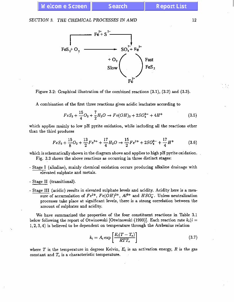
SECTION 3. THE CHEMICAL PROCESSES IN AMD 12
I Fss2-l FeS,+ 0, - SOi; Fe*+
+02
0
Fast
Slow FeS 2
Fe2 ’ .
Figure 3.2: Graphical illustration of the combined reactions (3.1), (3.2) and (3.3).
A combination of the first three reactions gives acidic leachates according to
Fe& + yO2 + SHzO + Fe(OH)s + 25’042- + 4H+ (3.5)
which applies mainly to low pH pyrite oxidation, while including all the reactions other than the third produces
Fe& + YOz + TFe3’ + 4 ‘7Hz0 + F Fe*+ + 2SO42- + 4 ‘7H+ (3.6)
which is schematically shown in the diagram above and applies to high pH pyrite oxidation. Fig. 3.3 shows the above reactions as occurring in three distinct stages:
- Stage I (alkaline), mainly chemical oxidation occurs producing alkaline drainage with
elevated sulphate and metals.
- Stage II (transitional).
- Stage III ( aci ic results in elevated sulphate levels and acidity. Acidity here is a mea- d )
sure of accumulation of Fe*+, Fe(OH) 2+ A13+ and HSOh. Unless neutralization ,
processes take place at significant levels, there is a strong correlation between the
amount of sulphates and acidity.
We have summarized the properties of the four constituent reactions in Table 3.1 below following the report of Otwinowski [Otwinowski (1993)]. Each reaction rate ki(i = 1,2,3,4) is believed to be dependent on temperature through the Arrhenius relation
ki = Aiexp [ EiE&oTo)] (3.7)
where T is the temperature in degrees Kelvin, E; is an activation energy, R is the gas constant and To is a characteristic temperature.

SECTION 3. THE CHEMICAL PROCESSES IN AMD 13
F%(a) + ‘4 Op + t$O - F.+2+ ~SQ-~+ 2H+ 4 .
fita+ sl_o- + SH+
.
i Fo +2 + l/,0,+ H+ - F.+’ + ‘/zH2Q
Log Ti +2
1 FeS# + 14F.+3+ t3fi20 LlSF. -2 + 2% 4
+ ld n
Figure 3.3: Stages in the formation of acid rock drainage following ref. 16.
3.3 Acid Neutralization
On the other hand, there exist several acid consuming minerals, such as calcite (CaCOs) and gibbsite (Af(OH3)) that neutralize the products of oxidation through the following types of reactions:
C&O&) + H+ + Ca*+(aq) + HCO,(aq) (3.8)
or
and
CaCOs(s) + 2H+ -+ Cu*+(uq) + H2C0,(uq) (3.9)
AZ(OH)3 + 3H+ + A13+ + 3H20. (3.10)
The balance between the two types of processes (acid production and acid neutralization) determines the net amount of acidity.
As was mentioned earlier, our interests lie in studying the kinetics of the chemical reactions discussed here and in the determination of the influence of both external condi- tions and internal composition on the overall rate of ARD. In the next section we derive

SECTION 3. THE CHEMICAL PROCESSES IN AMD
Rate
ICI = 2.83 x 10-gcm-1/2s-’ =.
clep~nds on pH
kzr = 1.66 x 10-gatm-‘s”
for pH 5 3.5; To = 25°C k = 4:: x low6 M-‘aim-‘s-’ for
pH < 2; To = 30°C k 23 =
, 1.33 x 10¹³M-2atm-1s-1 for
Activation Energy
Er = 57 f 7.5kJ/mol
E21 = 74 kJ/mol for pH < 3.5
~922 = 85 kJ/mol for
3.5 < pH < 5
E23 = 96 kJ/mol for
pH>5
E., = 90 kJ/mol.
14
pH-dependence
pH independent up to pH=7.
pH independent up to pH=3.5. first order w.r.t. OH- for
3.5 < pH < 5.
second order w.r.t. OH- for
pH > 5.
strongly pH dependent
complicated
Table 3.1: A summary of characteristic properties of the four reactions in eqs. (3.1)-(3.4) following Otwinowski (1993).
the equations governing the nonlinear chemical kinetics for both acid generation and acid neutralization processes. This will be followed by numerical modelling under a diverse
range of conditions.
. . .

Section 4
Modelling and Its Results
In this section we set up the equations for the chemical kinetics of the AMD problem and then provide a host of numerical results obtained under different conditions. We analyze separately the two groups of reactions, i.e.: (a) acid production and (b) neutralization
reactions. In the last subsection we deal with the issue of the modelling of chemical reactions occurring in porous media.
4.1 Acid Production (Homogeneous Medium)
The four reactions studied here are:
kr 2FeSz + 702 + 2HsO +
k-1
k2 4Fe2+ + 02 + 4H+ +
k-2
ks Fe3+ •t 3H20 +
k-3
h Fe& + 14Fe3+ + 8H2O +
k-4
2Fe2+ + 4SO,2- + 2H+ (4.1)
4Fe3+ + 2H20
Fe(OH)3 + 3H+
15Fe2+ + 2S02- + 16H+. 4
(4.2)
(4.3)
V-4)
For the sake of convenience we introduce the following notation for the concentrations of the chemical species present
X1 E [Fe&]; X2 G [Oz]; Xs z [HzO]; X4 G [Fe’+]; X5 E [SO,2-]; X6 G [H+]; X7 F [Fe3+]; X8 I [Fe(OH)a]
For all practical purposes the above reactions are not reversible due to the large free energy of reaction involved. Since our analysis did not become much more complicated by the inclusion of reverse reactions and we set out to investigate the most extreme role nonlinearity may play, we nonetheless performed several simulation with the presence of
15

SECTION 4. MODELLING AND ITS RESULTS 16
reverse reactions. Based on the discussion provided in the previous section we set up the
equations of chemical kinetics for these processes as follows: .
x, = -k X2X27X; - kdXlX;4Xi 1 1 (4.5)
.
x2 = -;klXTx,?X; - k2X,4X2X,4 (4.6)
23 = -k1X;X;X; + 2k2XjX2X; - k3X7X; - 8k4X1X;4X; (4.7) x4 = klX;X;X; - 4k2X;X2X; + 15k4X1X;4X~ (4.8) . x, = 2k1X;X;X; + 2k4X1X;4X; (4.9) . X6 = 11 k X2X,7X,2 - 4k2X,4X2X,4 + k3X7X; + 16k4XlX;4Xi (4.10)
X7 = 4k2X;X2X; - fk,X,X; - 14k4XrX;“X~ (4.11) .
x#J = W& (4.12)
Note that at this stage we have not included the possibility of either reverse reactions, or inflows into and outflows out of the system. The above equations automatically satisfy mass balance and we checked it numerically for all our solutions. We should make here an important qualification. The equations we derived above are only valid for elementary reactions. in reality, the stoichiometric coefficients imposed above can not be used a priori as the order of reactions for complex reactions. Hence, the order of reactions must be determined empirically. This effectively means that the approach we present here is simplified for the purpose of making the analysis easily tractable. It represents the most extreme scenario from the point of view of nonlinearity of the equations studied. However, at present we are unable to make the analysis more realistic for the lack of reliable experimental data.
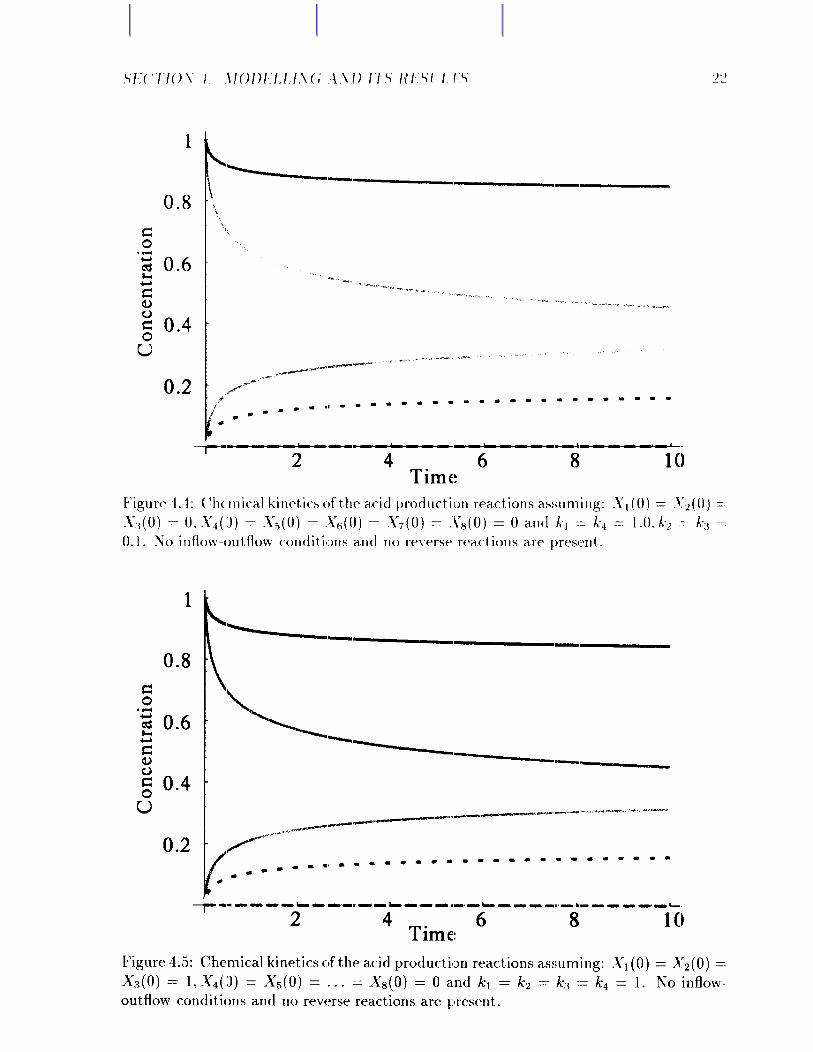
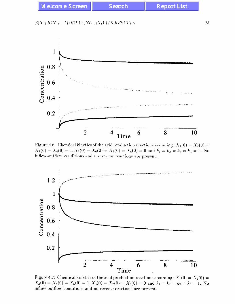
Having no precise knowledge regarding the reaction rates we have run several trial computations with a range of test values of both initial values of concentrations and reaction rate magnitudes. Our findings are illustrated in Figs. 4.1-4.8. In Fig. 4.1- 4.8 (and also further below) we have normalized the concentrations of all the chemical species {X1, . . . , Xs} to be within the 0 to 1 range, 0 meaning complete depletion and 1 complete saturation. This has been dictated by expediency and simplicity. We do not have precise knowledge of the abundances and reaction rates but at this stage we were mainly interested in qualitative behavior. The time variable is also scaled and is represented in
arbitrary units. However, in reality the time units will be those of the slowest reaction in the chain. Comparing with Figs. 5.1-5.4 we can make an educated guess and identify one time unit in our diagrams with approximately 10-15 days of real time. The initial
points (ie. those at t = 0) were selected in several possible ways in order to examine various feasible situations. For example, it was commonly assumed that FeS2, 02 and Hz0 are initially at their saturation levels while the remaining five species are, in the beginning, not present. As the reader may see from the figure captions, other possibilities were also considered. The reaction rates were all set at unity except for Fig. 4.4 where
k2 = k3 = 0.1 (with very little change in the qualitative behavior). The numerical codes used in these simulations are very reliable and give consistant, reproducible results. We have a measure of confidence in our findings and intend to perform more computations with different input data in the future. As the reader may easily appreciate, the problem is not computational in nature, but rests with obtaining a reliable set of empirically-based
input data.

SECTION 4. MODELLING AND ITS RESULTS 17
We have studied the above equations under a number of different conditions as well. What emerges, however, can be summarized as a rather smooth and regular tendency of all the chemical species involved to reach their equilibrium concentrations. This is the case whether we change the initial concentrations or vary the reaction rates for the various reactions. Therefore, at this stage of modelling complete predictability of these processes seems virtually guaranteed and no hallmarks of chaos or irregularity have been found.
In the next step of our investigation we attempted to find out if the behavior of the system significantly changes when reverse reactions are allowed to take place. To this end
we assumed that Ic_s # 0 and k-3 # 0 leaving k-1 = k_q = 0. The relevant equations are different and they now become
-klX;Xz’X; - k$&X;4X: (4.13)
-;klX,aX:x,2 - kzX,“XzX6” + ksX;X; (4.14)
-krX;X;X,2 + 2kzX,4XzX,4 - 3&i& - 8k,XrX:4X:
-2k2X;X; + 3k&X,3 (4.15)
klX;X;X; - 4kzX,4XzX, + 15k,X,X;4X: + 4k-sX;X: (4.16)
2klX;X;X; + 2k,X,X:4X,s (4.17)
k x2x;X; - 4k2X:X2X: + 3rc,X& + 16k4X1X:4X,8 1 1
+4k_2X;X,2 - 3k.e,X,X: (4.18)
4k2XiX2X,4 - ksX7X; - 14k4X1X;4X,8 - 4k_2X;X: + k-3X8X,3 (4.19) kzX,X; - k-.3X&,3 (4.20)
A sample result of our numerical simulation of this system is shown in Fig. 4.9 where we have exaggerated the effect somewhat by assuming that the reverse reaction rate is half of the forward rate. Nevertheless, what we obtained indicates a by and large smooth behavior and, again, a tendency towards equilibration . There is a short-lived period of non-monotonic behavior close to the beginning of the process but it rapidly gives way to the asymptotic trend towards equilibrium.
In the final stage of modelling the acid production processes we allow the presence of inflows into or outflows from the system. This applies to the abundances of water and oxygen. As a result, the only reactions that are affected by this change of prevailing conditions are
. x2 = -;klX;X;X; - k2X;X2X; + k_m2X;X; - f2(X2 - X2) (4.21)
Jts = -klX;X;X; + 2k2X,4X2X; - 2k_2X;X; - 3kzX7X,3
+3k_3X,X,3 - 8k4X,X;4X,8 - f2(Xs - Xs) (4.22)
where fs and fs are the mean flow rates for oxygen and water, respectively, while X2 and Xs represent the equilibrium values of the oxygen and water concentrations, respectively.
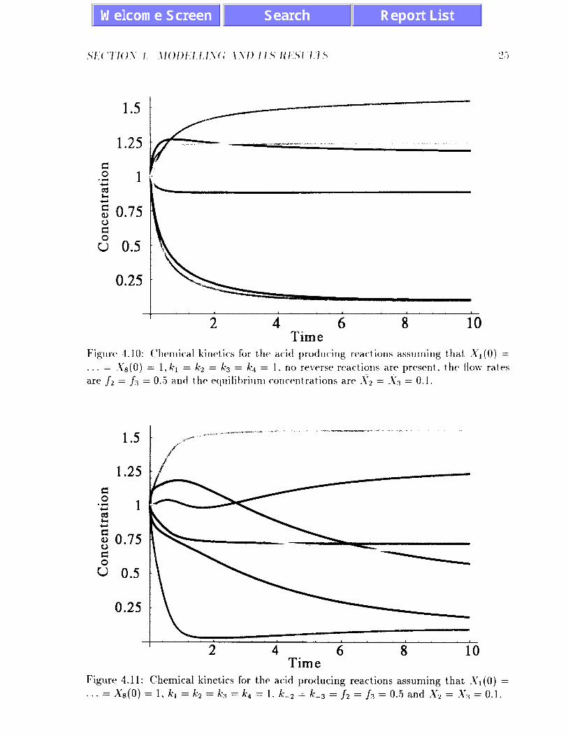
What follows is a selection of modelling results for a variety of initial conditions, reaction rates and flow rates. Fig. 4.10 illustrates the effect of flow rates on the the mica1 kinetics. It is assumed here that no reverse reactions are present. Note again the smoothness and regularity of the resultant behavior.

SECTION 4. MODELLING AND ITS RESULTS 18
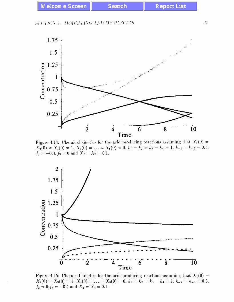
In Figs. 4.11-4.18 we illustrate the behavior when both reverse reactions and flow rates are nonzero. The first group of diagrams shows the chemical kinetics for positive flow rates (Figs. 4.11-4.13) while the second group (Figs. 4.13-4.18) allows one or both of the flow rates to be negative.
To summa&e our findings in this part we emphasize the very sensitive dependence of the chemical kinetics on the flow rates. This is evident for both positive and negative flow rates. In the former case, a drastic difference is clearly seen in the intermediate time range on going from Fig. 4.11 to Fig. 4.12 resulting from a change in the magnitudes of fs and fs. Asymptotically, however, positive flow rates result in a long-range smooth relaxation towards equilibrium concentrations. On the other hand, when one or two flow rates become negative, this leads to the emergence of divergent behavior in the associa ted generation of a given species. Simultaneously, the irregular, non-monotonic region of behavior is substantially extended in time.
4.2 Acid Production (Porous Medium)
As discussed in subsection 2.2, the net result of porosity in the medium where chemical reactions take place is that the reaction rates become strongly time dependent. It was argued earlier in this report that to effectively account for the porosity aspect of the medium, the chemical reaction studied must be assumed to have reaction rates such that [Kopelman (1986)]
ki = /+-‘I3 (i = 1,2,3,4). (4.23)
In order to study this effect we repeated our numerical modelling with the above conditions .
built into the coupled equations for chemical kinetics. Our results are summarized in Figs. 4.19-4.22:
What emerges from the diagrams above is an even more sensitive dependence on the flow rates for these reactions in a porous medium as compared to a homogeneous medium. Regions of transient non-monotonic behavior are extended in the time domain and much of the regularity has been removed. Strictly speaking, the long-time behavior presented in Figs. 4.20-4.22 contradicts the assumptions built into the model since some of the concentrations involved exceed their saturation values of one. One can deal with this by either further resealing or a change in the initial conditions or, finally, by restricting the time variable. It should also be added that all these diagrams involve inflow-outflow conditions and hence the total mass is not conserved within the system over time.
An interesting observation based on this set of simulations can be made that the
prevelence of monotonic growth or depletion characteristic of homogeneous models is here destroyed by the assumption that the medium is porous. The fractality of the rock (see discussion in Sec. 5.3) implies time-dependent reaction rates which lead to often non-monotonic chemical kinetics. It appears obvious, however, in view of earlier remarks that the scaling laws such as eq. (4.23) should have validity over a limited range of time, or conversely should be tempered by saturation factors.

SECTION4. MODELLINGANDITSRESULTS
4.3 Acid Neutralization Reactions
19
The main acid neutralization reactions are
CaCOs+H+ 3 Ca2++HCO;
CaC03+2H+ 3 Ca'++H&Os
AZ(OH)s+3H+ 3 A13++3Hz0
(4.24)
(4.25)
(4.26) (4.27)
where Ki, K2 and K3 axe the associated reaction rates. For simplicity, we have introduced the following symbols for the concentrations of the chemical species present:
Yr E [CaCOs]; Y2 G [H+]; y3 = [Ca2+]; I$ z [HCO,]; I$ = [H2C03]; yS s [Al(OH)s]; Y,= [AZ"+]; yS = [Hz01
Using the same technique as in the preceding subsections we derive the kinetic equa- tions for acid neutralization as
. Yi = .
Yz = .
Ys = .
Y4 = .
Ys = .
Ys = .
Yr = .
Ys =
-K,Y,Y, - K2YlY22 (4.28)
-KlYlY2 - 2K2YrY; - 3KsYeY; (4.29)
KI y,y2 + KzKY,~ (4.30)
KlKy2 (4.31)
K2W2 (4.32)
-K3YsY23 (4.33)
K3&Y,3 (4.34)
2K3YsY: (4.35)
This system is much simpler than the one for acid production and the order of non- linearities is also significantly reduced. In fact, due to their structure, the equations on Ys, Y4, Ys and Yr are effectively decoupled from the remaining three and the dynamics is governed by the equations on Yr, YZ and Ys; the other four concentrations are solely determined by the results from the interplay between Yr, Y2 and Ys. Not surprisingly, our numerical modelling of the acid neutralization reactions produced a very smooth and predictable behavior. This is illustrated on a sample result given in Fig. 4.23. We see that all the species concentrations follow monotonic curves to their equilibrium values. We conclude that the process of acid neutralization should be primarily determined by the abundance of CaC03, H+ and the equilibrium reaction rates. No indications ofnon- linear stochastic or chaotic behavior have been found and no challenges to the problem of predictability seem to be offered by this set of reactions. This is, of course, in contrast to the acid production reactions discussed above where a substantial amount of unpre- dictability exists due primarily to the two factors: (a) porosity of the medium and (b) flow rates of oxygen and water. Note that acid,neutralization reactions do not seem to be dynamically coupled to the reactions of acid production. It is probably safe to assume that pH oscillations that can be observed just prior to acid generation are a result of this setup. Thus, such oscillations could be considered a good-predictor of the onset of AMD
process.

3)
Xl FeS2
x6 H+
x8
(‘olor I,cgcnd for E’ig1lres ,l. 1 1.22.
4 6 8 10 Time
Figure 3.1: Chemical kinetics of the acid production reactions assuming: Sl(O) = X2(0) =
X3(O) = _Y7(0) = l._Y4(0) = S,(O) = X6(O) = ,Ys(O) = 0 and k-1 = k2 = k3 = k-4 = 1. No
inflow--outflow conditions a.nd no reverse rextions are present.
Con
cent
ratio
n 0
0 0
0 id
b
in
ia
0 C
I
1
0.2
. .__. ^__ _._ __-
4 Time
6 8 10
Figure 4.6: C’hemica.1 kinetics of t.hc acid production reactions assuming: .Y, (0) = .Yz(O) =
X3(0) = Xi,(O) = l._YS(O) = X6(0) = X7(0) = .Ys(O) = 0 and xj = x’2 = k-3 = k4 = 1. No
inflow-outflow conditions and no reverse react ions are present.
Time _
Figure 4.7: Chemical kinet,ics of the acid production rextions a.ssuming: S,(O) = S,(O) =
_Y3(0) = -Y*(O) = X5(O) = 1,X6(O) = _Y7(0) = A’s(O) = 0 and ATI = X:2 = !Q = kq = 1. No inflow-outflow conditions and no reverse react,ions are present.

i .-4 --ii -fi -
10 Time
Figure .4.8: Chemical kinetics of the acid production rmctions assunling: S,(O) = .4’*(O) =
X3(0) = _&j(O) = l,.&(O) = S,(O) = S;(O) = &q(O) = 0 and k, =r A-2 = x-3 = A.4 = 1. No j
inflowout flow conditions and no reverse react ions are presmt .
Figure 4.9: Chemical kinetics of the acid production reactions assuming t’hat lY1(0) =
. . . = _Y~(O) =l:k, =k2=k3=k4=1 arldk--2=k_-3=0.q5.
4 Time
6 8
.)- _.)
1.5
1.25
Ef .3 1 s b 2 0.75
2 w 0.5
0.25
Time Figure 4.10: (‘liemica kinetics for the a,cid producing rca.ct,ions a.ssuming t.hat -Y,(O) =
. . . = X8(0) = 1.k1 = ka = A.3 = A.4 = 1. no reverse rea.ctiolls xc present. the flow rates
are .fi = j-T = 0..5 and t,hc equilibrium concentrations are s, = _Y3 = 0.1.
0.25
~.,“.,,,,,,,,, ,, ,,*,, ,, 2 4 6 8 10
Time Figure 4.11: Chemical kinetics for the acid producing rea,ctions assurlling that, S,(O) =
. . . = .&(O) = 1. kl = k2 = kg = kd = 1, k-2 = k_g = f2 = f3 = 0.5 and .y, = A& = 0.1.

3
0.5
4 6 8 10 Time
Figure 1.12: (‘hemical kinetics for t>he acid producing reactions assuming t,hat .YI(0) =
. . . = &(O) = 1. k, = k-2 = ko = k-4 = 1. k-2 = k_:s = 0.5. j-2 = j-3 = 1.0 a.r1d
_y, = x3 = 0.5.
1
0.8
Figure 4.13: Chemical kinetics for the acid producing react,ions assuming tha.t ?r’l(O) =
X2(0) = X,(O) = 1, &(O) = . . . = X8(O) = 0. kl = k2 = k3 = k4 = 1. k_z = k_g = f;! = f3 = 0.5 and ?Lrz = _J?, = 0.1.
Time Figure 4.13: Cherrlic-al kinetics for t,hc acid producing rea.ctions assuming that *Y,(O) =
X2(0) = X3(0) = 1. X4(0) = . . . = .Ys( 0) = 0. xj = x.2 = I& = /Cd = 1 . k-2 = x*-:3 = 0..5.
FL = -0.4, jz3 = 0 a,nd X2 = X3 = 0.1.
2
1.75
1.5
2 1.25 ‘S z % 1
2 0.75
G 0.5
0.25
4 6 8 10 Time
Figure 4.15: Chemical kinetics for the acid producing reactions a.ssuming t,hat, .Y1(0) =
X2(0) = X3(0) = 1: S,(O) = . . . = &3(O) = 0. ccl = k2 = k‘s = k:4 = 1. k-2 = Ic-g = 0.5,
j’2 = O;fs = -0.4 and _y2 = .?, = 0.1.
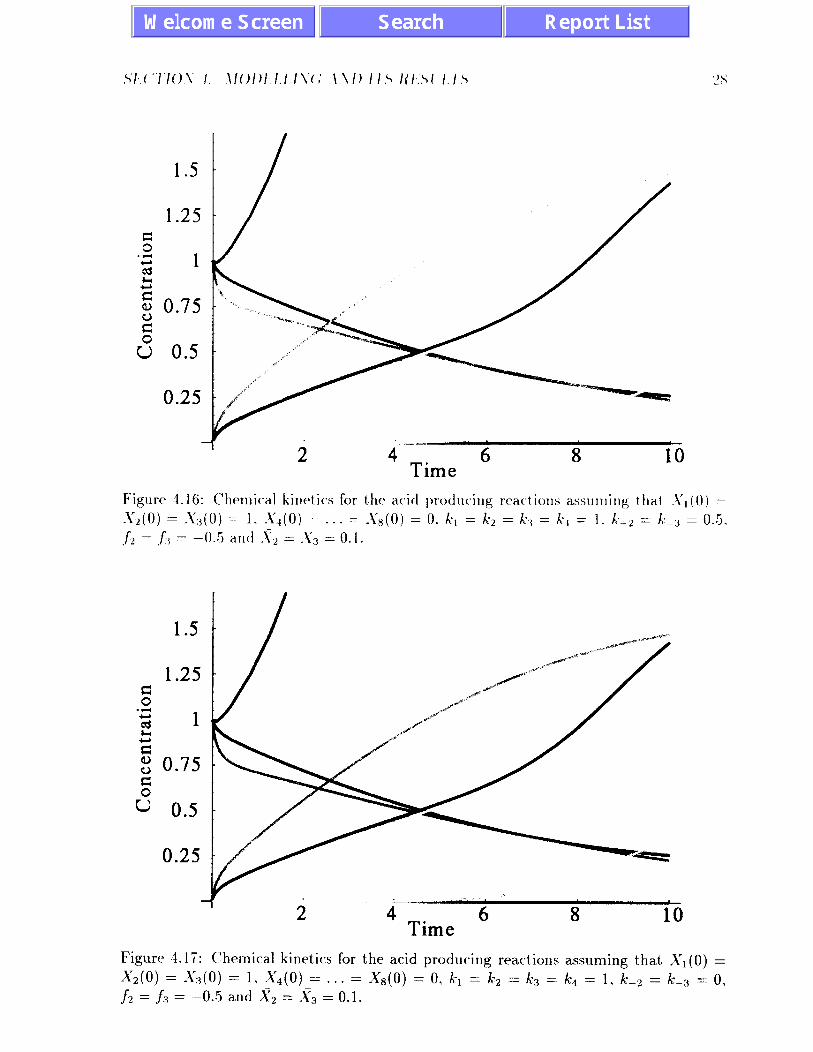
Figure 4.16: (‘llernical kiIlc>t its for the acid producing react ions a.ssuInirig that -Y,(O) =
X’;?(O) = &(O) = 1. S,(O) = . . . = ,& (0) = 0. I;, = A.2 = /$, = x.1 = 1 . k-2 = A.__3 = 0..5,
Ji = .j.. = -0..5 and .U, = .Ys = 0. I.
1.5
0.25
Figure 4.17: Chemical kinetics for the a.cid producing reactions assuming t’hat Sl(O) =
&(O) = X3(0) = 1, X4(0) = . . . = X8(O) = 0. kl = k2 = kg = k4 = 1. k_2 = k_3 = 0, fi = f3 = --0..5 and Xx = X3 = 0.1.

L’!)
Figure 1.18: Chemical kinetics for the acid producing reactions assunling tt1a.t S,(O) =
Sz(O) = X,(O) = 1. X,(O) = . . . = S,(O) = 0. A-1 = k2 = k-3 = k-4 = 1. k-2 = k-:3 = 0,
.f2 = -0.5. and .f3 = 0 a.nd .T:, = _Y:i = 0.1.
1
0.2
~.rrr=~rrr.r,rrrr.~r....~.~~~.~
2 4 Time
6 8 10
Figure 4.19: Chemical kinetics for the acid producing rexCons in a porous medium with
the assumption that, S,(O) = X2(0) = X3(0) = 1, X4(0) = . . . = X8(0) = 0. f2 = f3 = 0.5
and s2 = .??s x 0.5.

:io
2
1.5 s .d 5
-_._ l. _,.j . .
c
2 4 6 8 10 Time
Figure 4.20: C’hemical kinetics for t.he acid producing react,ions in a porous medium wit811
the a.ssrrrrrption that S,(O) = . . . = S,(O) = l..fi = J3 = O.:i and _Y2 = _I’:3 = 0.5.
2 4 6 Time
8 10
Figure 3.21: Chemical kinetics for the acid producing reactions in a porous medium with the assumption that A’,(O) = . . . = Xs(0) = 1, f2 = 0..5, f3 = -O.F, and .T2 = X3 = 0.5.

.S/..‘f “/‘/O.\ I \Io/)I:/./,I.~(; \ \I) 17,s /I/...SI -/./.s :I I
1.75
Figure 4.22: ~‘llemical kinetics for t,he xid producing reactions in a porous medium with
the assumption tha,t .X,(O) = . . . = S,( 0) = 1, &* = -0..5. & = 0.5 a.nd .Yz = xig = 0.*5.
Al(OH)
CaCO 3
HCO;
H2O
WO 3
At+
Time
Figure 4.23: Chemical kinetics of the acid neutralization process where we have assumed
that YI(0) = Y2(0) = &(O) = l,yy(O) = E;(O) = k’;(O) = IS_(O) = Ii(O) = 0, and that
I-I-~ = h =2 = hp:3 = 1.

Section 5
Discussion and Future Outlook
5.1 Summary and Conclusion
The present report has outlined the activity that has been undertaken within the frame- work of the above project.
First of all, a very extensive literature survey encompassing both geochemical analyses regarding the acid mine drainage problem and the relevant aspects of nonlinear chemical kinetics has been carried out. We have found detailed analyses regarding the primary chemical reactions involved in acid production. Qualitative aspects of chemical kinetics, such as which reactions are slow and which ones are fast can be readily found in the literature. Detailed characteristics in terms of activation energies and reaction rates were independently described by Dr. M. Otwinowski who submitted a parallel report.
In terms of nonlinear chemical kinetics we now have all the required information needed to solve the problem at hand. Several factors emerged as important theoretical considerations which were included in the numerical work described above. These are: (i) inflow-outflow ratios for water which will be strongly correlated with the porosity of the rock and seasonal variations such as rainfall, (ii) porosity of the medium, in contrast to the rather crude assumption about its homogeneity has been included in our model. Moreover, the inclusion of uncatalyzed reactions may be of importance in modelling, . We found that the effect of medium’s porosity and size distribution of the rock can be accounted for by introducing time-dependent reaction rates. The time dependence required takes the form of power laws with exponents that are functions of the fractal dimension. The latter, in turn, is a characteristic quantity defining the structure of the rock and must be determined experimentally first (see Sec. 5.3).
The second stage of our work consisted in analyzing in detail the chemical kinetics in the AMD problem. We have set up the kinetic equations for the concentrations of the compounds involved. Two groups of equations have been investigated separately. In the acid production stage we found 8 coupled differential equations (highly non- linear) for the concentrations of: Fe,!& 02, HZO, Fe2+, SO:-, H+, Fe3+ and Fe(OH)s and describing their time evolution. However, the last equation for Fe(OH)s is ef-
fectively decoupled from the rest making the system consist of 7 first-order ordinary
differential equations. One of the results of this stage of chemical activity enters into
the second stage, i.e. acid neutralization which is, otherwise, independent of the pre-
vious process. The acid neutralization stage involves 7 different concentrations, i.e.:
CaCOs, H+, Ca2+, HCO,, H2CO3, AZ(OH)3 and Al 3+ The seven kinetic equations we .
32
SECTION 5. DISCUSSION AND FUTURE OUTLOOK 33
have set up are also nonlinear but this time the problem is substantially reduced as four of the equations decouple from the rest. Thus, we obtained just 3 coupled equations. This part of the project has been completed by building mass balance into the equations, carrying out dimensional analysis to maximally simplify the mathematical problem at hand and looking for steady states. No interesting steady-state solutions appear to exist other than complete depletions of reactants.
The third part of the problem has been to set up the numerical machinery at our disposal. With the newly acquired Next Work Station (including a laser printer) and the great time involvement of the students MLAN and DS, the required numerical code has been written and tested and many results obtained. Our results can be summarized as follows. Although the kinetic equations derived are highly nonlinear, no hallmarks of bifurcations or chaotic dynamics were found thus far. This would indicate the question of predictability is perhaps not as comphcated as it could at first appear. However, we have also detected the presence of complex, non-monotonic behavior of the concentrations of the chemical species involved under special circumstances. This irregular behavior seems to be mainly affected by two factors:
(i) the porosity of the medium (ii) the presence of non-zero flow rates of oxygen and water.
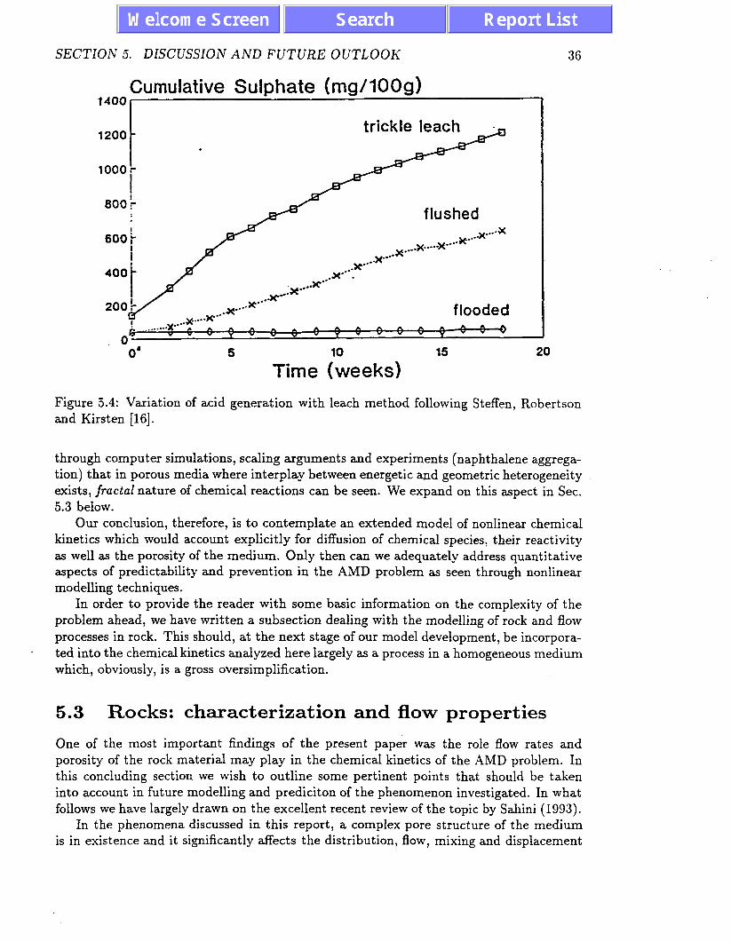
Thus, depending on the physical structure of the waste rock, specifically depending on the level of its inhomogeneity, the production of acid may follow a different course, being more regular in time for a more homogeneous medium than in a fractal-like distribu- tion of waste rocks. Moreover, the flow rates of oxygen and water affect the reactions very significantly and they are certainly related to both climatic changes (rainfall, hu- midity) as well as the waste rock shape and structure, especially vis a vis the exposure to oxygen. Support of this conclusion can be found in the work of Doepker and Drake
[Doepker et al.(1991)] h w ere significantly different effects of leaching have been obtained
between air-exposed and water-submerged tailings. Similarly, Steffen, Robertson and
Kirsten[RPWQM Rep. No. 1952011 h s ow a marked difference in the production of SO4
between flooded and unflooded test samples. In numerous cases sulphate production kinetics exhibits a smooth, relaxation-type
behavior with time. Test results shown by Steffen, Robertson and Kirtsten [RPWQM Rep. No. 1952011, Denholm and Hallan [Denholm (1991)], Bradham and Caruccio [Bradham et al.] and Fergusen and Morin [Ferguson et al.] all indicate largely regular time dependence of SO4 production and CaCOs dissolution. We have reproduced below some of the plots presented by these authors. This is consistent with the bulk of our
results. We should add a word of caution here regarding the predictability of AMD as based
on purely physico-chemical models. As can be seen from Fig. 3.1, the biological activity of microorganisms present in the environment adds a whole new dimension to the analysis and could effectively alter the end results in terms of the release time and the amount of acjd produced. What we wish to rather emphatically stress, however, is that in spite of the highly nonlinear characteristics of the chemical kinetics involved, the observed processes
are very regular. No hallmarks of chaos, quasi-periodicity or intermittency have been found. Thus these phenomena should be very easy to model and predict provided reliable input data are available in terms of initial concentrations, reaction rates, flow rates and
the structural properties of the medium. Therein lies the challenge of predictability and we believe that with steady progress in understanding the processes involved in AMD we
SECTION 5. DLSCUSSION AND FUTURE OUTLOOK 34
400
200
n -0 10 20 30 40 so 00 70 no 90 100 110
hmpla W*dt
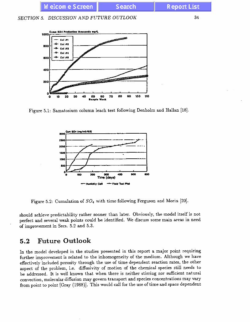
Figure 5.1: Samatosium column leach test following Denholm and Hallan [18].
Figure 5.2: Cumulation of SOS with time following Ferguson and Morin [20].
should achieve predictability rather sooner than later. Obviously, the model itself is not
perfect and several weak points could be identified. We discuss some main areas in need of improvement in Sets. 5.2 and 5.3.
5.2 Future Outlook
In the model developed in the studies presented in this report a major point requiring further improvement is related to the inhomogeneity of the medium. Although we have effectively included porosity through the use of time dependent reaction rates, the other aspect of the problem, i.e. diffusivity of motion of the chemical species still needs to
be addressed. It is well known that when there is neither stirring nor sufficient natural convection, molecular diffusion may govern transport and species concentrations may vary from point to point [Gay (1988)]. Th is would call for the use of time and space dependent

SECTION 5. DISCUSSLON AND FUTURE OUTLOOK 35
WEh
- CIN
0 60 100 150 Total Days
250
Figure 5.3: Plot of cumulative acidity for acidic weathering cells following Bradham and Caruccio [ 191.
concentration fields Xi(t, 2) and Yi (t, _) x in the acid production and acid neutralization reactions studied in this report.
We should mention that Davis and Hitchie [Davis et al. (1986)] have developed a series of models simulating diffusion into rock piles. The initial model, called the simple homogeneous model, simulated oxygen differences from the top of a pile downwards to oxidation sites. The model equations were solved assuming pseudo-steady -state diffusion
within the particles. However, this and all the subsequent models[Morin et al. (1990)] were based on a linear diffusion equation of the type:
Where D, is the effective diffusion constant, C is the oxygen concentration and R is the rate of Oz uptake. As demonstrated by Prigogine and many other reseachers [Glansdorff et al. (1971)], a more appropriate description for reaction-diffusion equations calls for the use of nonlinear coupled partial differential equations of the form
dll at = f(u) + DV’u (5.2)
where D is a diffusion constant [Kuramoto (1984)] and f( ) u is a nonlinear function coup- ling the species involved according to reaction kinetics. Depending on the particulars of the system, a reaction-controlled, a diffusion-controlled or an intermediate regime may prevail. Both oscillatory and chaotic temporal regimes may exist and spatial patterns show amazing complexity exhibiting propagating and standing wave behavior, rotating spiral formation[Henze et al. (1990)] as well as chemical turbulence. Bifurcations are known to occur resulting from unequal diffusion coefficients for the individual reactions. Importantly to our problem, observations of such behavior have been.made for heteroge- neous processes occurring at gas-solid and liquid-solid interfaces, e.g. catalytic oxidation
of CO on Pt (110) single crystal surfaces. In a recent study [Ertl (1991)] it was shown
SECTION 5. DISCUSSlON AND FUTURE OUTLOOK
Cumulative Sulphate (mg/lOOg) 1400
1200-
flushed
flooded
0’ 5
Time &eels) 15 20
36
Figure 5.4: Variation of acid generation with leach method following Steffen, Robertson and Kirsten [lS].
through computer simulations, scaling arguments and experiments (naphthalene aggrega- tion) that in porous media where interplay between energetic and geometric heterogeneity exists, fructal nature of chemical reactions can be seen. We expand on this aspect in Sec. 5.3 below.
Our conclusion, therefore, is to contemplate an extended model of nonlinear chemical kinetics which would account explicitly for diffusion of chemical species: their reactivity as well as the porosity of the medium. Only then can we adequately address quantitative aspects of predictability and prevention in the AMD problem as seen through nonlinear modelling techniques.
In order to provide the reader with some basic information on the complexity of the problem ahead, we have written a subsection dealing with the modelling of rock and flow processes in rock. This should, at the next stage of our model development, be incorpora- ted into the chemical kinetics analyzed here largely as a process in a homogeneous medium which, obviously, is a gross oversimplification.
5.3 Rocks: characterisation and flow properties
One of the most important findings of the present paper was the role flow rates and porosity of the rock material may play in the chemical kinetics of the AMD problem. In this concluding section we wish to outline some pertinent points that should be taken into account in future modelling and prediciton of the phenomenon investigated. In what follows we have largely drawn on the excellent recent review of the topic by Sahini (1993).
In the phenomena discussed in this report, a complex pore structure of the medium is in existence and it significantly affects the distribution, flow, mixing and displacement

SECTION 5. DISCUSSION AND FUTURE OUTLOOK 37
of fluids present. Various physical mechanisms play a role, such as heat and mass trans- fer, thermodynamic phase behavior, forces of viscosity, buoyancy, gravity and capillarity making the analysis especially demanding. For reactive fluids, the pore structure of the medium may even change due to the reactions of the fluid with the rock surface. A crucial point to emphasize here is that the analysis performed depends on several length scales over which the porous medium may or may not be regarded as homogeneous.
When there are inhomogeneities in the system that persist over various length scales, the overall behavior is dependent on transport processes (diffusion, conduction, convec- tion) and morphology. The general classes of porous media distinguished are: (a) micro- scopically disordered but macroscopically homogeneous (characterized by size-independent
transport properties) and, (b) macroscopically hetrogeneous (with several types of trans- port properties).
To model transport processes in porous media, two types of approaches have been adopted: (a) continuum models; and (b) discrete models. However, only in the past fifteen years have modern ideas from statistical physics been applied to flow, dispersion and displacement processes in porous rocks. Such concepts as percolation, fractality, self-similarity and pattern formation are only now being implemented in the procedures used. We will discuss some of the repercussions that follow in the discussion below. For example, the pore volume and pore surfaces of many reservoir rocks are fractal and hence classical laws of physics have to be significantly modified. For instance, Fick’s law of diffusion with a constant diffusity is no longer applicable to diffusion processes in fractal systems. Instead, the diffusion coefficient becomes time- and space-dependent.
Porosity of reservoir rocks, ie. the volume fraction of their open space, has either a primary or a secondary origin. Primary porosity is due to ,the original pore space of the rock while secondary porosity is due to the chemical and physical changes through reactions with water.
The geometry of rock describes the shapes and sizes of its pores or fractures. In a porous medium, the space between its particles are called voids, whereas if the particles themselves are porous, then the void spaces in the particles are called pores. Pores can be divided into two groups: (a) pore bodies where most of the porosity originates, and (b) pore throats which are the channels that connect pore bodies. In a network representation of the pore space, the pore bodies are shown as sites or nodes while throats represent bonds of the network.
The pore size distribution is defined as the probability density-function that gives the distribution of pore volume by an effective pore size. Four main methods of measuring pore-size distributions are: (a) mercury porosimetry; (b) adsorption-desorption experi- ments; (c) small-angle scattering and (d) nuclear magnetic resonance.
In Fig. 5.5 we have shown a comparison between several types of porous media and theoretical simulation results. Fig. 5.6 illustrates pore-size distibution functions of sample
rocks. Pore-space models are required for calculating transport coefficients, permeability k
and other dynamical properties of porous media. The simplest property of a porous medium is its porosity 4. Relationships between k and 4 have been over the years proposed and tested, but there cannot be any general relationship between k and 4 since there exist porous media with the same 4 but different k.
In recent years it has been demonstrated that rock and other porous media (see Fig.
5.7) have fractal properties. There are six basic methods of measuring fractal proper-

SECTION5. DISCUSSIONANDFUTUREOUTLOOK 38
Quartzitic Sandstone Grain Consolidation
(b) Crystalline Dolomite Gaussian
Figure 5.5: Comparison of mathematical models and actual porous media.
ties: (a) the box method; (b) adsorption studies; (c) chord-length measurements; (d)
correlation function measurements, (e) small angle scattering and (f) spectral methods. In addition to fractality of the pores, fractal properties also characterize hetrogeneous
and fractured rocks. Fractures provide high permeability patterns for fluid flows and can be parameterized by fracture aperture, ie. the volumetric flow rate through a fracture (as a
function of aperture cubed). Fractures in a network appear to have different characteristics than isolated fractures. It was found that the frequency of inverse aperture y as a function of inverse aperture follows a power law, indicating fractality. Fractured rock has fractal geometry and is scale independent so that it can be represented by a singe1 parameter, the fractal dimension D defined as
bdN) D = log(l/l) (5.3)
where Nl is the number of fractures of length 1 (see Fig. 5.8). A study of the literature indicates the existence of three classes of models of fractured
rocks: (a) the classical multiporosity model, (b) network models of fractured rocks (frac- ta1 models) and (c) multifractal models. Many recent results definitely demonstrate the relevance of fractal statistics to modelling hetrogeneous media and especially transport processes in them. Simulations taking into account fractality lead to substantial improve- ments in the predictions of process performance. Fractal properties of the medium require the use of scale- and time-dependent dispersion coefficients as, for example, is the case with the typically-used convective diffusion equation
g+<v>TC=D d2C
Lo + W’:C (5.4)

SECTlON 5. DISCUSSION AND FUTURE OUTLOOK
_-
go. NUGGET SANDSTONE
80. +=17J- K - 282 md
70.
EFFECTIVE PORE RADII (pm)
s 90. BAKER DOLOMnE
EFFECTIVE PORE RADII (p-W
TUSCARORA SANDSTONE cc)
K = 0.05 md
EFFECTIVE PORE RADI! (pm)
loo1 DRUM UMESTONE
8 go- +- 16.1%
$ 80- K = 0.01 md
WI
” 01 ,-I 100 50 10 5 1 .5 ,l .05
EFFECTIVE PORE RADII &J-W
Figure 5.6: Pore-size distribution of various rocks.
where < v > is the macroscopic mean velocity, C the mean concentration of fluid, T and L stand for transverse and longitudinal direction, respectively. It is the objective
of modern techniques to determine the dependence of DL and DT on the nature of the porous medium present. Monte Carlo simulations demonstrate that dispersion coefficients
are scale dependent and for fractal hetrogenities grow with the distance travelled.

SECTION 5. DISCUSSION AND FUTURE OUTLOOK 40
H COCONINO
Figure 5.7: Typical fractal plot for Coconino sandstone .
10.
10' %
102
Figure 5.8: Fractal plot of surface fracture pattern.

SECTION 5. DISCUSSION AND FUTURE OUTLOOK 41
Acknowledgements
The authors with to thank Mr. B. Godin for his encouragement and for providing them with copies of numerous articles and reports that introduced them to the problem of AMD and its modelling. We also acknowledge valuable input given by Dr. R.V. Nicholson which resulted in significant improvements to the quality of this report.

An Introductory Overview of Nonlinear Phenomena
In the past two decades we have witnessed the emergence of new scientific paradigms that are making a revolutionary impact on the developments in the natural sciences. Such concepts as chaos, strange attractors, limit cycles and fractals are gradually taking root in the vocabulary of leading-edge scientists. The field of chemical kinetics has been an integral part of this new nonlinear science since its beginning. In the sections that follow
we provide a non-specialist overview of the key concepts required in the sophisticated modelling of nonlinear chemical kinetics. We begin by introducing the idea of chaotic behavior. This is followed by a subsection on coupled systems and Emit cycles. The question of predictability arises naturally and here we give the example of the Lorenz system where predictability is completely impossible. Having introduced these general concepts we proceed to discuss their relevance to chemical kinetics. In order to describe chemical kinetics in porous media we then introduce the concept of a fractal and the associated ‘idea of percolation. The final subsection deals with an emerging paradigm called pattern formation.
A: Chaotic Behavior
In the last few decades, the deterministic viewpoint of modem science has been challen- ged by the discovery of unstable dynamic, conservative systems with totally unpredictable behavior. The majority of dynamic systems, until a few years ago, ‘were thought to be ruled by deterministic laws and their behavior totally predictable. Unstable systems were considered to be an exception to the rule. However, very simple conservative sy- stems exist with few degrees of freedom which show sensitive dependence on the initial conditions and exhibit regimes of chaotic behavior. Their evolution may become unpre-
dictable in spite of an arbitrarily large amount of information we may have about them. Through it all they are indeed subject to the deterministic laws of classical dynamics! The so-called deterministic chaos arises as a result of simple, well-defined mathematical algorithms or equations, such as the logistic map investigated extensively by M. Feigen- baum [Baker et al. (1990), Cvitanovit (1984)]. Thi s is a rather simple iterative equation,
i.e.
%+l = rxn(l - xn) (A-1)
where f in the range: 0 < r c 4 is called a control parameter. For values of r < 3, the results eventually converge to a steady state called an attractor. However, for values of r > 3, the resultant oscillation does not settle down and remains stable, i.e. the behavior is periodic. The two possible values of z,,(r) never converge and the curve zn(r) shows what
42
AN INTRODUCTORY OVERVIEW OF NONLINEAR PHENOMENA 43
we call a bifurcation. Higher values of the control parameter r produce further splitting and doubling of the periodicities involved. Each period doubling is a bifurcation. If one plots the increasing control parameter r horizontally and the variable z, vertically, we obtain Fig. A.l. Abruptly, at r = 3.58, the result for x,, no longer oscillates periodically but changes in a chaotic fashion. The splittings, which started coming faster and faster for r > 3, are now squeezed together and the growth rate seems to. take any value at random.
Although for the values of r above rc chaos and randomness seem to prevail, a further increase of the control parameter, which makes the system even more nonlinear, introduces windows of regularity among chaos which is called intermittency. Computer simulations of the logistic map readily demonstrate (see the inset of Fig. A.l) that the structure is infinitely deep and self-similar. Parts of it, when magnified, show identical patterns, ad infinitum. These patterns (though in this example they come from a one-dimensional system) are a very common characteristic of the dynamic behavior of nonlinear systems leading to chaos and complexity. Bifurcations with successive, infinite period doubling
define one of the possible routes to chaos [Baker et al. (199O)j.
B: Coupled Systems and Limit Cycles
III chemical applications, in particular, the use of a single quantity (such as the variable x,) is inadequate as concentrations of several reacting chemical species must be described as independent variables. Here, instead of the well-studied relaxation dynamics characterized by an exponential time evolution towards, a steady-state attractor, a completely new type of behavior may arise. Specifically, a pattern of oscillating growth or extinction processes of individual species may be observed to act as a stable attractor. Perhaps the simplest example of such a cyclic population evolution can be found in the Lotka-Volterra model of prey and predator competition. Consider as a simple illustration the populations of
wolves (predator) and rabbits (prey) living in an isolated geographic area (e.g. an island) to limit the influences of other factors. Starting with a large population of wolves we readily predict a demise of rabbits as they will soon become an easy prey for the roaming
wolves. However, as soon as the rabbit population is decimated, the wolves will face
starvation leading to a downturn in their numbers. This, in turn, will allow rabbits to repopulate as they face a diminishing population of starved out wolves. As a consequence, a new phase in the development appears with numerous rabbits but few wolves. That will, of course, lead to a rapid repopulation of wolves and we have thus completed one cycle. This pattern repeats itself periodically.
In mathematical terms, we denote the concentration of each species (for example one type of reacting molecules) using a scalar timdependent variable, say ri(t), with 1 5 i 5 n denoting the number of species present. The time evolution of the entire
system is then governed by coupled first order differential equations of the general type [GlansdorfI et al. (1971), Kuramoto (1984)]
dz, - = f=({x;; 1 I i 5 n}) dt (B.1)
where fa is in general a function of all the concentrations involved and it usually contains

AN INTRODUCTORY OVERVIEW OF NONUNEAR PHENOMENA 44
a7 . 4.a I control
parameter
Figure A.l: The logistic map and its properties

AN INT_UODUCTORY OVERVIEW OF NONLINEAR PHENOMENA 45
significant nonlinearities. Take for example the following simple system [Hale et al. (1991)]
dxl dt = x2 + 051(x: + xi)
and
- = Xl +ax2(x: +x22) dt
(B.2)
(B.3)
where a is an adjustable constant (a control parameter). In fact, depending on the nu- merical value of this constant, three completely different types of behavior arise for the
solution set: xl(t),xs(t). In Fig. B.l we have shown phase portraits in each case, i.e. plotted the trajectories of {xl(t), x2(t)} with time t taken as a running parameter. When a < 0 a stable focus x1 = 0, x2 = 0 is found so that ail initial conditions lead to a spiralling
down on the focus point. When a = 0 all the orbits are stable circles since the system
can be represented as a harmonic oscillator. Finally, for a > 0 an unstable focus appears and all orbits diverge to infinity.
Figure B.l: The three possible
and (B.3).
.
behaviors in phase space for the solutions of eqs. (B-2)
I. Prigogine [Prigogine et al. . (1968)] studied a trimolecular model for a reaction in an
open system that can be schematically described by the reaction chain
h A +
k -1
k2
B+X + k-2
ks 2X+Y i=?
k-3
kd X +
k-4
X (B-4)
Y+D P.5)
3x (B-6)
E (B.7)
where A, B, D, E, X and Y denote various molecules, ICI, k2, k3, kd stand for forward while k_l, k_2, k_3, k_., for reverse reaction rates. This system has been referred to as the

AN INTRODUCTORY OVERVIEW OF NONUNEAR PHENOMENA . 46
Brusselator. In subsection 2.1 of the main text we demonstrate in detail how to derive the associated kinetic equations for the concentrations of X and Y molecules, denoted here for consistency by 51 and z2, respectively. They result in
da 2 -g = 51x2 - bxI + u - x1
and dx2 -= dt
-xix2 + bxl.
W)
(B-9)
What Prigogine noticed solving these equations (see Fig. B.2) was the presence of a (periodic) closed orbit in the phase space (xl, x2) to which all the neighboring trajectories are attracted. He called it a limit cycle and demonstrated its ubiquitous applicability as a self-sustaining pattern of oscillatory behavior. Prigogine’s discovery was revolutionary enough to the field of chemical kinetics that he was awarded a Nobel Prize in Chemistry.
Figure B.2: Trajectories obtained by numerical integration for the Brusselator reactions (B.4)-(B.7) for (1) X=Y=O; (2) X=Y=l; (3) X=10; Y=O; (4) X=1; Y=3.
More complicated nonlinear systems may possess a number of attractors (either point- like or limit cycles) and their trajectories may tend to one or more of them depending on
the initial conditions, i.e. their location with respect to the basins of attraction present [Glass et al. (1988) 1.
It could at first appear that all attractors in nonlinear dynamical systems have rather regular geometries. However, a large class of systems were discovered which display
attractors whose geometry is so complicated that it defies description. This is partly why this new type of attractor was called a strange attractor. In the next Appendix we discuss this novel nonlinear phenomenon.
c: Strange Attractors and Prediction Limitations
The MIT meteorologist E. Lorenz worked in the early sixties on simple models of atmos- pheric convection which results due to the daily operation of the Sun’s rays. He managed to simplify the problem to a system of just three coupled differential equations given below
dX - = b(X - Y) dt (C.1)

AN INTRODUCTORY OVERVIEW OF NONLJNEAR PHENOMENA .
wher and the t lineu decel Lorer He nc seemi to be the in wings long t
W: which had ve
Wes around I
fashion. of the Lc intersect infinite I the attra somewha contradic finite spa infinitely
Brusselator. In subsection 2.1 of the main text we demonstrate in detail how to ( the associated kinetic equations for the concentrations of X and Y molecules, de here for consistency by zi and ~2, respectively. They result in
hl _- = x 2
df ’ x2 - bxl + a - x1
and dxz -= dt
-xfxz + bxl.
What Prigogine noticed solving these equations (see Fig. B.2) was the present (periodic) closed orbit in the phase space (xi, x2) to which all the neighboring trajc are attracted. He called it a limit cycle and demonstrated its ubiquitous applicat a self-sustaining pattern of oscillatory behavior. Prigogine’s discovery was revolu enough to the field of chemical kinetics that he was awarded a Nobel Prize in Chl
Figure B.2: Trajectories obtained by numerical integration for the Brusselator (B.4)-(B.7) for (1) X=Y=O; (2) X=Y=l; (3) X=10; Y=O; (4) X=1; Y=3.
More complicated nonlinear systems may possess a number of attractors (ei like or limit cycles) and their trajectories may tend to one or more of them de: the initial conditions, i.e. their location with respect to the basins of attract (Glass et al. (1988)].
It could at first appear that all attractors in nonlinear dynamical systems regular geometries. However, a large class of systems were discovered wl attractors whose geometry is so complicated that it defies description. This ir this new type of attractor was called a strange attractor. In the next Appendi this novel nonlinear phenomenon.
c: Strange Attractors and Prediction Limit
The MIT meteorologist E. Lorenz worked in the early sixties on simple mod pheric convection which results due to the daily operation of the Sun’s rays. to simplify the problem to a system of just three coupled differential equation
dX - = c(X - Y) dt

AN INTRODUCTORY OVERVIEW OF NONLJNEAR PHENOMENA 48
e&t concept mentioned earlier. The fractal nature of a strange attractor introduces with it a non-integer dimension. Point attractors are zero-dimensional, limit cycles are of dimension one (curves) and quasi-periodic attractors (tori) are two-dimensional (surfaces). Curiously, the dimensionality of a strange attractor, as in general is the case for a fractal object, is a real, non-integer number, say 1.74. A number like this can be obtained through a rigorous algorithmic limit finding procedure which will be discussed in the next section which deals specifically with fractals. Instead of the traditional time series analysis, phase space trajectories revea 1 the implicate order present in chaotic dynamics. Fig., C.2 schematically juxtaposes both ways of presenting data for a variety of modes of behavior.
steady state limit cycle period three strange attractor
time series
. phase ’ portraits
Figure C.2: ‘Time-series versus phase-space characteristics for several nonlinear modes of behavior.
D: Fractals
Many pattern forming systems, especially when they are far from thermodynamic equi- librium, exhibit a growth of forms which are of fractal nature [Feder (1988)]. Specific examples include:
(4
04
(4
(4
Dendritic solidification in an undercooled medium;
Viscous fingering phenomena which occur when two fluids of different viscosities penetrate each other;
Aggregation phenomena such as diffusion-limited aggregation; and
Electrodeposition patterns of ions onto an electrode.
Some of these examples are graphically illustrated in Fig. D.l. The basic property of all fractal objects is their self-similarity, i.e. when we cut a part ’
of the object and then magnify it, the resulting objects appear the same as (or at least very similar to) the original object. Another property of fractals, which actually earned them

AN ZNTRODUCTORY OVERVIEW OF NONLINEAR PHENOMENA
(a) snowflake
(c) s&ace discharge
Figure D.l: Examples of fractals in nature.
(b) viscous fingering
their name; is that their dimensionality is not an integer but in general a real number. In the simplest form, the so-called fractal dimension D is given by the relationship
V(R) - R* (D-1)
where V(R) is the volume of the region bounded by the interface whose radius is R. The notion of fiactual especially as it pertains to geometrical objects was principally introduced into science by B. Man delbrot. It was subsequently studied by many physicists and generalizations of the definition were proposed, including multi-fractality. In the physical context it is useful to distinguish two general classes of fiactals:
(a) deterministic where a simple iterative rule is present, e.g. involving a procedure to cut a part of the object at each stage and replace it with a fixed element, and
(b) random where a stochastic approach is used so that a given operation, e.g. aggre- gation event, is predicted, with a preselected probability level.
Fractal objects can also be constructed algorithmically in two- or three-dimensional spaces. Two famous examples of fractal objects existing on a plane are the so-called Sierpinski gasket and the Sierpinski carpet (see Fig. D.2):
In a more rigorous sense, a fractal is a set of points in space for which the se&led HausdorE-Besicovitch dimension D strictly exceeds the topological dimension &. While the topological dime nsion is always an integer (1,2 or 3), the fractal dimension D is never an integer but a real number. The latter quantity expresses the property of size scaling

AN INTRODUCTORY
(a) Sieqinski gasket
OVERVIEW OF NONL3NlZAR PHENOMENA
(b) Siefpinskl e
50
D In3 = ln2 = 1.58... D In8
= In3= 1.89.w
Figure D.2: Two examples of mathematical fractals.
with the distance from the centre of a fractal object. The f&ctal dimension presents a way of quantifying properties that otherwise would have no clear definition. It expresses the degree of roughness or irregularity of a fractal object. In Figs. D.1 and D.2 we have given the fractal dimensions of the objects illustrated there.
E: Percolation Process
The concept of percolation was originaI.Iy introduced to deal with the process of spreading of a fluid through a random medium, for example oil or water in the pore space of a rock. In genera, the underlying mechanism of randomness in the process can be of 2 different types: (a) the classical diffusion process introduces randomness to the fluid, aud (b) the percolation process introduces randomness to the medium’s structure.
A site percolation problem is based on a network of lattice sites which are either occupied (probability p) or vacant (probability 1 - p). Two nearest-neighbor sites are called connected if they are both occupied. One similarly d&es a connected cluster. There is a site percolation threshold p, above which au infinite cluster of connected sites spans the network. In addition, one also defines the following important characteristics:
(9
(ii)
(iii)
(iv)
(v)
the percolation probability P(p) which character&s the probability that, when the fraction of occupied bonds is p, a given site belongs to the infinite cluster of occupied bonds.
the accesible fraction X*(p) is the fraction of coducting bonds belonging to the infinite cluster.
the backbone fraction XB(p) is the fraction of conducting bonds in the infinite ciu- ster which participate in conduction (ffow).
the correlation length tP(p) is the radius of the connected clusters for p < pc and the length scale over which the percolating network is homogeneous for p > pc.
the average number of clusters of size S, n,(p)
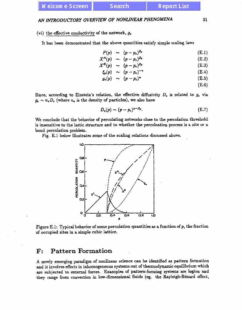
AN
(vi>
INTRODUCTORY OVERVIEW OF NONLINEAR PHENOMENA 51
the effective conductivity of the network, ge
It has been demonstrated that the above quantities satisfy simple scaling laws
P(P) - XA(P) - xw -
tPP(P> -
9ew -
(P - PcYP
(P - PJPP
(P - P2P
(P - PCY
(P - PC>’
Since, according to Einstein’s relation, the effective diffusivity D, is related to ge via ge N neDe (where n, is the density of particles), we also have
D,(p) - (p-~c)“+~. (E-7)
We conclude that the behavior of percolating networks close to the percolation threshold is insensitive to the lattic structure and to whether the percoloation process is a site or a
bond percolation problem. Fig. E.l below illustrates some of the scaling relations discussed above.
Figure E.l: Typical behavior of some percolation quantities as a function of p, the fraction of occupied sites in a simple cubic lattice.
F: Pattern Formation
A newly emerging paradigm of nonlinear science can be identified as pattern formation and it involves effects in inhomogeneous systems out of thermodynamic equilibrium which are subjected to external forces. Examples of pattern-forming systems are legion and they range from convection in low-dimensional fluids (eg. the Bayleigh-B&mud effect,
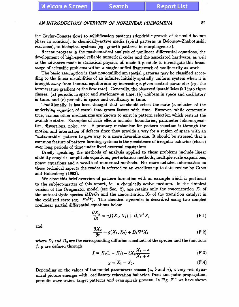
AN INTRODUCTORY OV~VZEW OF NONLINEAR PZ-ZENOUENA 52
the Taylor-Couette flow) to solidification patterns (dendridic growth of the solid helium phase in solution), to chemically-active media (spiral patterns in Belousov-Zhabotinskii reactions), to biological systems (eg. growth patterns in morphogenisis).
Recent progress in the mathematical analysis of nonlinear differential equations, the development of high-speed reliable numerical codes and the associated hardware, as well as the advances made in statistical physics, all made it possible to investigate this broad range of scientific problems within a single unified framework of nonlinearity at work.
The basic assumption is that nonequilibrium spatial patterns may be classified accor- ding to the linear instabilities of an infinite, initially spatially uniform system when it is brought away from thermal equilibrium by increasing a given control parameter (eg. the temperature gradient or the flow rate). Generally, the observed instabilities fall into three classes: (a) periodic in space and stationary in time, (b) uniform in space and oscillatory in time. and (c) periodic in space and oscillatory in time.
Traditionally, it has been thought that we should select the state (a solution of the underlying equation of state) that grows fastest with time. However, while commonly true, various other mechanisms are known to exist in pattern selection which restrict the available states. Examples of such effects include: boundaries, parameter inhomogenai-
ties, distortions, noise, etc.. A primary mechanism for pattern selection is through the motion and interaction of defects since they provide a way for a region of space with an “unfavorable” pattern to give way to a more favorable one. It should be stressed that a common feature of pattern-forming systems is the persistence of irregular bahavior (chaos) over long periods of time under fixed external constraints.
Briefly speaking, the methods of analysis applied to these problems include linear stability anaylsis, amplitude equations, perturbation methods,, multiple scale expansions, phase equations and a wealth of numerical methods. For more detailed information on these technical aspects the reader is referred to an excellent up-to-date review by Cross
and Hohenberg (1993). We close this brief overview of pattern formation with an example which is pertinent
to the subject-matter of this report, ie. a chemically active medium. In the simplest version of the Oregonator model (see Sec. 2), one retains only the concentration Xr of the autocatalytic species HBrOz and the concentration X2 of the transition catalyst in the oxidized state (eg. Fe3+). The chemical dynamics is described using two coupled nonlinear partial differential equations below
and
ax1 at = rf(& X2) + D1V2XI
ax2
-ar = g(& X2) + D2V2X2
(F.1)
(F.2) where Dr and D2 are the corresponding diffusion constants of the species and the functions
f, g are defined through X1-U
f=xl(1-xl)-bx2x1+a (F.3)
g=x, -x2. (F.4)
Depending on the values of the model parameters chosen (a, b and 7), a very rich dyna- mical picture emerges with: oscillatory relaxation bahavior, front and pulse propagation, periodic wave trains, target patterns and even spirals present. In Fig. F.l we have shown
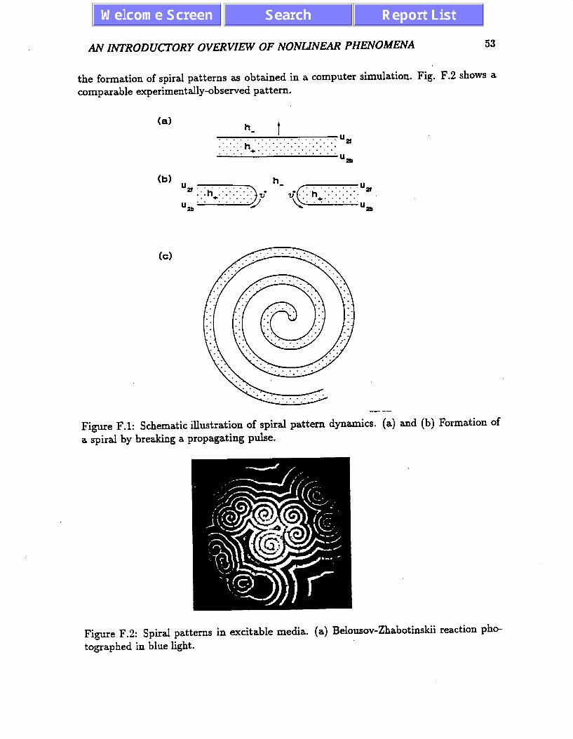
AN INTRODUCTORY OVERVIEW OF NONLJNEAR PHENOMENA 53
the formation of spiral patterns as obtained in a computer simulation. Fig. F.2 shows a comparable experimentally-observed pattern.
(a)
(b)
(4 . . . . . . . . . . . . . . . . . . . . . . . . CD3 . . _ . . . . . . . . . :‘ . . _-.
Figure F.l: Schematic illustration of spiral pattern dynamics. (a) a spiral by breaking a propagating pulse.
and 04 Formation of
Figure F.2: Spiral patterns in excitable media. (a) Belousov-Zhabotinskii reaction pho tographed in blue light.

List of Figures
2.1
3.1 3.2 3.3
4.1
4.2
4.3
4.4
4.5
4.6
4.7
4.8
4.9
A schematic of a continuous-flow stirred reactor. . . . . . . . . . . . . . . . 5
Sulphide oxidation as a function of pH following ref. 16. . . . . . . . . . . 11
Graphical illustration of the combined reactions (3.1), (3.2) and (3.3). . . . 12
Stages in the formation of acid rock drainage following ref. 16. . . . . . . . 13
Chemical kinetics of the acid production reactions assuming: X,(O) =
X2(0> = Xs(0) = X7(0) = 1,X4(0) = Xs(0) = X6(0) = Xs(0) = 0 and ICI = k2 = k3 = k4 = 1. No inflow-outflow conditions and no reverse
reactions are present. . . . . . . . . . . . . . . . . . . . . . . . . . . . . . . 20 Chemical kinetics of the acid production reactions assuming: X1(O) =
X2 (0) = Xs(0) = Xs(0) = 1,X4(0) = Xs(0) = X6(0) = XT(O) = 0 and kl = k2 = k3 = k4 = 1. No inflow-outflow conditions and no reverse
reactions are present. . . . . . . . . . . . . . . . . . . . . . . . . . . . . . . 21 Chemical kinetics of the acid production reactions assuming: X1(O) = X2(0) = . . . = X8(0) = 1 and ICI = k2 = ka = k4 = ‘1. No inflow-outflow conditions and no reverse reactions are present. . . . . . . . . . . . . . . . 21
Chemical kinetics of the acid production reactions assuming: Xl(O) =
X2 (0) = Xs(0) = 0,X4(0) = Xs(0) = Xs(0) = XT(O) = Xs(0) = 0 and kl = k4 = 1.0, k2 = kg = 0.1. No inflow-outflow conditions and no reverse reactions are present. . . . . . . . . . . . . . . . . . . . . . . . . . . . . . . 22 Chemical kinetics of the acid production reactions assuming: X1(O) = X2(0) = Xs(0) = 1,X4(0) = X5(0) = . . . = Xs(0) = 0 and kl = k2 = k.3 = k4 = 1. No inflow-outflow conditions and no reverse reactions are present. . 22
Chemical kinetics of the acid production reactions assuming: X,(O) = X2(0) = X3(O) = X4(O) = 1,X5(0) = X6(0) = XT(O) = X8(O) = 0 and ICI = k2 = k3 = k4 = 1. NO inflow-outflow conditions and no reverse
reactions are present. . . . . . . . . . . . . . . . . . . . . . . . . . . . . . . 23 Chemical kinetics of the acid production reactions assuming: X1(O) = X2(0) = Xs(0) = X4(0) = Xs(0) = 1,X6(0) = X7(0) = X*(O) = 0 and kl = k2 = k3 = k4 = 1. No inflow-outflow conditions and no reverse
reactions are present. . . . . . . . . . . . . . , . . . . . , . . . . . . . , . . 23 Chemical kinetics of the acid production reactions assuming: X1(O) = X2(0) = Xs(0) = Xc(O) = 1,X4(0) = Xs(0) = X7(0) = Xs(0) = 0 and ICI = k2 = kg = k4 = 1. No inflow-outflow conditions and no reverse
reactions are present. . . . . . . . . . . . . . . . . . . . . . . . . . . . . . . 24 Chemical kinetics of the acid production reactions assuming that Xl(O) = . . . = X8( 0) = 1, ICI = k2 = k3 = k4 = 1 and k-2 = k_3 = 0.5. . . . . . . . . 24
54

LIST OF FIGURES 55
4.10 Chemical kinetics for the acid producing reactions assuming that X,(O) = . . . = Xs(0) = l,lcr = IcZ = k3 = k4 = 1, no reverse reactions are present, the flow rates are fi = fs = 0.5 and the equilibrium concentrations are XZ=Xs=O.l. . . . . . . . . . . . . . . . . . . . . . . . . . . . . . . . . . 25
4.11 Chemical kinetics for the acid producing reactions assuming that X1(O) = . . . = X*(O) = 1, k1 = kz = kz = kd = 1, k_2 = k-3 = fi = f3 = 0.5 and XZ=Xs=O.l. . . . . . . . . . . . . . . . . . . . . . . . . . . . . . . . . . 25
4.12 Chemical kinetics for the acid producing reactions assuming that X1(O) = . . . = X*(O) = 1, ICI = k2 = k3 = kq = 1, k-2 = kq = 0.5, fi = f3 = 1.0 andXs=Xs=0.5.. . . . . . . . . . . . . . . . . . . . . . . . . . . . . . . 2G
4.13 Chemical kinetics for the acid producing reactions assuming that X1(O) = X2(O) = X3(O) = 1, X4(O) = .._. = J+(O) = 0, kl = kg = k3 = k4 = 1, k-2 = k-3 = f2 = f3 = 0.5 and X2 = Xs = 0.1. . . . . . . . . . . . . . . . . 26
4.14 Chemical kinetics for the acid producing reactions assuming that X,(O) = X2(0) = Xs(0) = 1, X4(0) = . . . = Xs(0) = 0, ICI = k2 = kg = k4 = 1, k-g = k_3 = 0.5, fi = -0.4, f3 = OandXz=Xs=O.l. . . . . . . . . . . . 27
4.15 Chemical kinetics for the acid producing reactions assuming that X1(O) = X2(0) = Xs(0) = 1, X4(0) = . . . = X8(O) = 0, k1 = kz = k3 = k4 = 1, k = k_3 = 0.5, f2 = O;fs = -0.4 and Xs = Xs = 0.1.
4.16 Ch?mical kinetics for the acid producing reactions assummg‘that XI(O) = ’ 27
X2(O) = Xa(0) = 1, X4(O) = . . . = Xs(0) T 0, kl = k2 = kg = k4 = 1, k_2 = k_3 = 0.5, fi = f3 = -0.5 and X, = Xs = 0.1. . . . . . . . . . . . . 28
4.17 Chemical kinetics for the acid producing reactions assuming that X1(O) = X2(O) = X3(O) = 1, X4(O) = . . . . = X*(O) = 0, ICI = kz = k3 = k4 = 1, k_z = k_3 = 0, fi = f3 = -0.5 and X, = Xs = 0.1. . . . . . . . . . . . . . 28
4.18 Chemical kinetics for the acid producing reactions assuming that X1(O) =
X2(0) = Xs(0) = 1, X4(0) = . . . = Xs(0) = 0, kl = k2 = k3 = k4 = 1,
k_p = k_3 = 0, f2 = -0.5, and f3 = 0 and Xz = X, = 0.1. . . . . . . . . . 29
4.19 Chemical kinetics for the acid producing reactions in a porous medium with the assumption that Xl(O) = X2(0) = Xs(0) = 1,X4(0) = . . . = Xs(0) = 0,fi=fs=0.5andXZ=Xs=0.5.. . . . . . . . . . . . . . . . . . . . . . 29
4.20 Chemical kinetics for the acid producing reactions in a porous medium with the assumption that X,(O) = . . . = Xs(0) = 1, fi = f3 = 0.5 and X,=X,=0.5. . . . . . . . . . . . . . . . . . . . . . . . . . . . . . . . . . 30
4.21 Chemical kinetics for the acid producing reactions in a porous medium with the assumption that Xl(O) = . . . = Xs(0) = 1, fi = 0.5, f3 = -0.5 andXs=Xs=0.5.. . . . . . . . . . . . . . . . . . . . . . . . . . . . . . . 30
4.22 Chemical kinetics for the acid producing reactions in a porous medium with the assumption that Xl(O) = . . . = Xs(0) = 1, fi = -0.5, f3 = 0.5 andXs=Xs=0.5.. . . . . . . . . . . . . . . . . . . . . . . . . . . . . . . 31
4.23 Chemical kinetics of the acid neutralization process where we have assumed that Y,(O) = Ys(0) = Ye(O) = l,Ys(O) = Yd(O) = Ys(0) = Y,(O) = Ys(0) = 0, and that Kr = K2 = Ks = 1. . . . . . . . . . . . . . . . . . . . . . . . . 31
5.1 Samatosium column leach test following Denholm and Hallan [18]. . . . . . 34 5.2 Cumulation of SO4 with time following Ferguson and Morin [20]. . . . . . 34

LIST OF FIGURES 5G
5.3
5.4
5.5 5.6 5.7 5.8 A.1 B.l
B.2
c.1 c.2
D.l D.2 E.l
F.l
F.2
Plot of cumulative acidity for acidic weathering cells following Bradham and Caruccio [19]. ................................ 35
Variation of acid generation with leach method following Steffen, Robertson and Kirsten [16]. ................................ 36
Comparison of mathematical models and actual porous media. ....... 38
Pore-size distribution of various rocks. .................... 39
Typical fractal plot for Coconino sandstone ................... 40
Fractal plot of surface fracture pattern. .................... 40
The logistic map and its properties ...................... 44
The three possible behaviors in phase space for the solutions of eqs. (B.2) and(B.3). .................................... 45
Trajectories obtained by numerical integration for the Brusselator reactions (B.4)-(B.7) for (1) X=Y=O; (2) X=Y=l; (3) X=10; Y=O; (4) X=1; Y=3. . 46
The strange attractor of Lorenz. ........................ 47
Time-series versus phase-space characteristics for several nonlinear modes of behavior. ................................... 48
Examples of fractais in nature. ......................... 49
Two examples of mathematical fractals. .................... 50
Typical behavior of some percolation quantities as a function of p, the fraction of occupied sites in a simple cubic lattice. .............. 51
Schematic illustration of spiral pattern dynamics. (a) and (b) Formation of a spiral by breaking a propagating pulse. ................. 53
Spiral patterns in excitable media. (a) Belousov-Zhabotinskii reaction pho- tographed in blue light. .... , ......................... 53

LIST OF FIGURES 56
5.3
5.4
5.5
5.6 5.7 5.8 A.1 B.l
B.2
c.1 c.2
D.l D.2 E.l
F.l
F.2
Plot of cumulative acidity for acidic weathering cells following Bradham and Caruccio [19]. . . . . . . . . . . . . . . . . . . . . . . . . . . . . . . . . 35 Variation of acid generation with leach method following Steffen, Robertson and Kirsten [16]. . . . . . . . . . . . . . . . . . . . . . . . : . . . . . . . . i3
Comparison of mathematical models and actual porous medra. . . . . . . .
Pore-size distribution of various rocks. . . . . . . . . . . . . . . . . . . . . 39 Typical fractal plot for Coconino sandstone . . . . . . . . . . . . . . . . . . . 40 Fractal plot of surface fracture pattern. . . . . . . . . . . . . . . . . . . . . 40 The logistic map and its properties . . . . . . . . . . . . . . . . . . . . . . 44 The three possible behaviors in phase space for the solutions of eqs. (B.2) and (B.3). . . . . . . . . . . . . . . . . . . . . . . . . . . . . . . . . . . . . . 45
Trajectories obtained by numerical integration for the Brusselator reactlons (B.4)-(B.7) for (1) X=Y=O; (2) X=Y=l; (3) X=10; Y=O; (4) X=1; Y=3. . 46
The strange attractor of Lorenz. . . . . . . . . . . . . . . . . . . . . . . . . 47 Time-series versus phase-space characteristics for several nonlinear modes of behavior. , . . . . . . . . . . . . . . . . . . . . . . . . . . . . . . . . . . 48
Examples of fractals in nature. . . . . . . . . . . . . . . . . . . . . . . . . . 49 Two examples of mathematical fractals. . . . . . . . . . . . . . . . . . . . . 50 Typical behavior of some percolation quantities as a function of p, the fraction of occupied sites in a simple cubic lattice. . . . . . . . . . . . . . . 51 Schematic illustration of spiral pattern dynamics. (a) and (b) Formation of a spiral by breaking a propagating pulse. . . . . . . . . . . . . . . . . . 53 Spiral patterns in excitable media. (a) Belousov-Zhabotinskii reaction pho tographed in blue light. . . . . , . . . . . . . . . . . . . . . . . . . . . . . . . 53

References
[ARDPM]
[Baker et al. (1990)]
[CvitanoviC (1984)]
[Glansdorff et al. (1971)]
[Kuramoto (1984)]
[Hale et al.’ (1991)]
[Prigogine et al. (1968)]
[Glass et al. (1988)]
[Feder (1988)]
[Gray (1988)l
[Richetti et al.]
[Vidal et al. (1984)]
[Kopelman (1986)]
[DARDTG v. l]
Acid Rock Drainage Prediction Manual (Department of Energy, Mines and Resources, Vancouver, 1990).
G.L. Baker and J.P. Gollub, Chaotic Dynamics (Cambridge Univ. Press, Cambridge, 1990).
P. CvitanoviC, Universality in Chaos (Adam Hilger Ltd. Bristol, 1984).
P. Glansdorff and I. Prigogine, Thermodynamic Theory of Structure, Stability and Fluctuations (Wiley-Interscience, Lon- don 1971).
Y. Kuramoto, Chemical Oscillations, Waves and Turbulence (Springer, Berlin, 1984).
J. Hale and H. Kocak, Dynamics and Bifurcations (Springer- Verlag, New York, 1991).
I. Prigogine and R. Lefevre, J. Chem. Phys. 48, 1695 (1968).
L. Glass and M.C. Mackey, From Clocks to Chaos (Princeton Univ. Press, Princeton, 1988).
J. Feder, Fractals (Plenum Press, New York, 1988).
P. Gray,“Instabilities and Oscillations in Chemical Reactions in Closed and Open Systems”, Proc. Roy. Sot. Lon. A 415, 1
(1988).
P. Richetti and A. Arneodo, The Periodic-Chaotic Sequences in Chemical Reactions: A Scenario Close to Homoclinic Condi- tion, preprint.
C. Vidal and A. Pecault (eds.) Non-Equilibrium Dynamics in Chemical Systems (Springer, Berlin, 1984).
R. Kopelman, J. Stat. Phys. 42, 185 (1986).
Draft Acid Rock Drainage Technical Guide Vol. 1 (British Co- lumbia Acid Mine Drainage Task Force, Vancouver, 1989).
57
REFERENCES 58
[RPWQM Rep. No. 1952011 Rock Pile Water Quality Modelling. Report No. 195201,
[Otwinowski (1993)]
[Denholm (1991)]
[Bradham et al.]
[Ferguson et al.]
[Henze et al. (1990)]
[Ertl (1991)]
[Davis et al. (1986)]
[Morin et aI. (199O)j
[Cross et al. (1993)]
[Sahini (1993)]
[Jaynes et al. (1984)]
[Scharer et al. (1993)]
[Doepker et al.( 1991)]
Steffen, Robertson and Kirsten, Oct. 1992.
M. Otwinowski, Quantitative Analysis of Chemical and Biolo- gical Kinetics for the Acid Mine Drainage Problem, preliminary progress report (1993).
E. Denholm and R. Hallan, a review of Acid Generation Rese- arch at the Samatosum Mine, in 1991 MEND Conference Pro- ceedings, Montreal, Sept. 16-18, 1991, Vol. 2, p.561.
W.S. Bradham and F.T. Caruccio. a Comparative Study of Tai- lings Analysis Using Acid Base Accounting, Cells, Columns and Soxhlets, ibidem, Vol.1, p.157.
K.D. Ferguson and K.A. Morin, The Prediction of Acid Rock Drainage - Lessons from the Data base, ibidem, Vol. 3, p.83.
C. Henze, E. Lugosi and A.T. Winfree, Can. J. Phys. 68, 683 (1990).
G. Ertl, Science 254, 1750 (1991).
G.B. Davis and A.I.M. Ritchie, Appl. Math. Model. 10, 314;
323 (1986).
K.A. Morin, E. Gevencher, C.E. Jones, D.E. Konasewich, J.R. Harries, Critical Literature Review of Acide Drainage From
Waste-Rock. Draft Report, May 1990.
M.C. Cross and P.C. Hohenberg, Rev. Mod. Phys. 65, 851 (1993).
M. Sahini, Rev. Mod. Phys. 65, 1393 (1993).
D.B. Jaynes, AS. Rogourski and H.B. Pionke, Water Resources Research 20, 233 (1984).
J.M. Scharer, R.V. Nicholson, B. Halbert and W.J. Snodgrass, A Computer Program to Assess Acid Generation in Pyritic Tai- lings, Proc. ACS Symposium of Environmental Geochemistry of Sulphide Oxidation (1993).
R.D. Doepker and P.L. Drake, Laboratory Study of Submer- ged Metal-Mine Tailings 3: Factors Influencing the Dissolution of Metals, Proc. Second Int. Conf. on the Abatement of Acid
Drainage, Vol 1 (1991)