arX

iv:1

703.

0116

4v1

[cs

.RO

] 3

Mar

201

7

Nonlinear Model Predictive Control for Multi-Micro Aerial Vehicle

Robust Collision Avoidance

Mina Kamel∗, Javier Alonso-Mora†, Roland Siegwart∗, and Juan Nieto∗

∗Authors are with the Autonomous Systems Lab, ETH Zurich†Author is with the Delft Center for Systems and Control, TU Delft

Abstract— Multiple multirotor Micro Aerial Vehicles (MAVs)sharing the same airspace require a reliable and robust collisionavoidance technique. In this paper we address the problemof multi-MAV reactive collision avoidance. A model-basedcontroller is employed to achieve simultaneously referencetrajectory tracking and collision avoidance. Moreover, we alsoaccount for the uncertainty of the state estimator and the otheragents position and velocity uncertainties to achieve a higherdegree of robustness. The proposed approach is decentralized,does not require collision-free reference trajectory and accountsfor the full MAV dynamics. We validated our approach insimulation and experimentally.

I. INTRODUCTION

As the miniaturization technology advances, low cost and

reliable MAVs are becoming available on the market with

powerful on-board computation power. Many applications

can benefit from the presence of such low cost systems such

as inspection and exploration [1], [2], surveillance for secu-

rity [3], mapping [4] or crop monitoring [5]. However, MAVs

are limited to short flight times due to battery limitation and

size constraints. Due to this limitation, creating a team of

MAVs that can safely share the airspace to execute a specific

mission will widen the range of applications where MAVs

can be used and will be beneficial for time-critical missions

such as search and rescue operations [6].

A crucial problem when multiple MAVs share the same

airspace is the risk of mid-air collision, because of this, a

robust method to avoid multi-MAVs collisions is necessary.

Typically, this problem is solved by planning collision-free

trajectory for each agent in a centralized manner. However,

this binds the MAVs to the pre-planned trajectory and limits

the adaptivity of the team during the mission: any change

in the task will require trajectory re-planning for the whole

team.

In this work we present a unified framework to achieve

reference trajectory tracking and multi-agent reactive col-

lision avoidance. The proposed approach exploits the full

MAV dynamics and takes into account the physical platform

limitations. In this way we fully exploit the MAV capabilities

and achieve agile and natural avoidance maneuvers compared

to classic approaches, where planning is decoupled from

trajectory tracking control. To this end, we formulate the

control problem as a constrained optimization problem that

we solve in a receding horizon fashion. The cost function of

the optimization problem includes a potential field-like term

that penalizes collisions between agents. While potential field

methods do not provide any guarantee and are sensitive to

Fig. 1: An instance of the experimental evaluation of multi-agentcollision avoidance proposed strategy.

tuning parameters, we introduce additional tight hard con-

straints to guarantee that no mid-air collisions will occur. The

proposed method assumes that each agent is broadcasting its

position and velocity on a common network. Additionally, to

increase the avoidance robustness, we use the state estimator

uncertainty to shape the collision term in the cost function

and the optimization constraints.

The contribution of this paper can be summarized as

follows:

i A unified framework for multi-agent control and collision

avoidance.

ii The incorporation of state estimator uncertainty and

communication delay for robust collision avoidance.

This paper is organized as follows: In Section II we present

an overview of existing methods for multi-agent collision

avoidance. In Section III we briefly present the MAV model

that will be considered in the controller formulation. In

Section IV we present the controller and discuss the state

estimator uncertainty propagation. Finally, in Section V we

present simulation and experimental results of the proposed

approach.

II. RELATED WORK

Many researchers have demonstrated successful trajectory

generation and navigation on MAVs in controlled envi-

ronment where obstacles are static, using external motion

capture system [7] or using on-board sensing [8]. Sampling

based planning techniques can be used to generate global

collision-free trajectories for single agent, taking into account

the agent dynamics [9] and static and dynamics obstacles in

the environment.

One way to generate collision-free trajectories for a team

of robots is to solve a mixed integer quadratic problem in a

centralized fashion as shown in [10]. A similar approach was

presented in [11] where sequential quadratic programming

techniques are employed to generate collision-free trajec-

tories for a team of MAVs. The aforementioned methods

lack real-time performance and do not consider unforeseen

changes in the environment.

Global collision-free trajectory generation methods limit

the versatility of the team of robots. In real missions, where

multiple agents are required to cooperate, the task assigned

to each agent might change according to the current situa-

tion, and reactive local trajectory planning methods become

crucial.

One of the earliest works to achieve reactive collision

avoidance for a team of flying robots in a Nonlinear Model

Predictive Control (NMPC) framework is the work presented

in [12] where a decentralized NMPC is employed to control

multiple helicopters in a complex environment with an arti-

ficial potential field to achieve reactive collision avoidance.

This approach does not provide any guarantees and has been

evaluated only in simulation. In [13] the authors present

various algorithms based on the Velocity Obstacles (VO)

concept to select collision-free trajectories from a set of

candidate trajectories. The method has been experimentally

evaluated on 4 MAVs flying in close proximity and including

human. However, the MAV dynamics are not considered

in this method, and decoupling trajectory generation from

control has various limitations as shown in the experimental

section of [13].

Among the attempts to unify trajectory optimization and

control is the work presented in [14]. The robot control

problem is formulated as a finite horizon optimal control

problem and an unconstrained optimization is performed at

every time step to generate time-varying feedback gains and

feed-forward control inputs simultaneously. The approach

has been successfully applied on MAVs and a ball balancing

robot.

In this work, we unify the trajectory tracking and collision

avoidance into a single optimization problem in a decen-

tralized manner. In this way, trajectories generated from a

global planner can be sent directly to the trajectory tracking

controller without modifications, leaving the local avoidance

task to the tracking controller.

III. MODEL

In this section we present the MAV model employed in

the controller formulation. We first introduce the full vehicle

model and explain the forces and moment acting on the

system. Next, we will briefly discuss the closed-loop attitude

model employed in the trajectory tracking controller.

1) System model: We define the world fixed inertial frame

I and the body fixed frame B attached to the MAV in the

Center of Gravity (CoG) as shown in Figure 2. The vehicle

configuration is described by the position of the CoG in the

inertial frame p ∈ R3, the vehicle velocity in the inertial

Bx

Bz

By

Fi

Ix

Iy

Iz

FT,i

Faero,i

v

v⊥

−mgIp,RIB

ni

Fi

Fig. 2: A schematic of MAV showing Forces and torques acting onthe MAV and aerodynamic forces acting on a single rotor. Inertialand CoG frames are also shown.

frame v, the vehicle orientation RIB ∈ SO(3) which is

parameterized by Euler angles and the body angular rate ω.

The main forces acting on the vehicle are generated from

the propellers. Each propeller generates thrust proportional

to the square of the propeller rotation speed niand angular

moment due to the drag force. The generated thrust FT,i and

moment Mi from the i− th propeller is given by:

FT,i = knn2i ez, (1a)

Mi = (−1)i−1kmFT,i, (1b)

where kn and km are positive constants and ez is a unit

vector in z direction. Moreover, we consider two impor-

tant effects that appear in the case of dynamic maneuvers.

These effects are the blade flapping and induced drag. The

importance of these effects stems from the fact that they

introduce additional forces in the x − y rotor plane, adding

some damping to the MAV velocity as shown in [15]. It is

possible to combine these effects as shown in [16], [17] into

one lumped drag coefficient kD .

This leads to the aerodynamic force Faero,i:

Faero,i = fT,iKdragRTIBv (2)

where Kdrag = diag(kD, kD, 0) and fT,i is the z component

of the i− th thrust force.

The motion of the vehicle can be described by the follow-

ing equations:

p = v, (3a)

v =1

m

(

RIB

Nr∑

i=0

FT,i −RIB

Nr∑

i=0

Faero,i + Fext

)

+

00−g

, (3b)

RIB = RIB⌊ω×⌋, (3c)

Jω = −ω × Jω +A

n21

...

n2Nr

, (3d)

where m is the mass of the vehicle and Fext is the external

forces acting on the vehicle (i.e wind). J is the inertia matrix,

A is the allocation matrix and Nr is the number of propellers.

2) Attitude model: We follow a cascaded approach as

described in [18] and assume that the vehicle attitude is

controlled by an attitude controller. For completeness we

quickly summarize their findings in the following paragraph.

To achieve accurate trajectory tracking, it is crucial for

the high level controller to consider the inner loop system

dynamics. Therefore, it is necessary to consider a simple

model of the attitude closed-loop response. These dynamics

can either be calculated by simplifying the closed loop

dynamic equations (if the controller is known) or by a

simple system identification procedure in case of an unknown

attitude controller (on commercial platforms for instance).

In this work we used the system identification approach to

identify a first order closed-loop attitude response.

The inner-loop attitude dynamics are then expressed as

follows:

φ =1

τ φ(kφφcmd − φ) , (4a)

θ =1

τ θ(kθθcmd − θ) , (4b)

ψ = ψcmd, (4c)

where kφ, kθ and τφ, τθ are the gains and time constant of

roll and pitch angles respectively. φcmd and θcmd are the

commanded roll and pitch angles and ψcmd is commanded

angular velocity of the vehicle heading.

The aforementioned model will be employed in the subse-

quent trajectory tracking controller to account for the attitude

inner-loop dynamics. Note that the vehicle heading angular

rate ψ is assumed to track the command instantaneously. This

assumption is reasonable as the MAV heading angle has no

effect on the MAV position.

IV. CONTROLLER FORMULATION

In this section we present the unified trajectory tracking

and multi-agent collision avoidance NMPC controller. First,

we will present the Optimal Control Problem (OCP). After-

wards we will discuss the cost function choice and the state

estimator uncertainty propagation to achieve robust collision

avoidance. Next, we will present the optimization constraints

and finally we will discuss the approach adopted to solve the

OCP in real-time on-board of the MAV.

A. Optimal Control Problem

To formulate the OCP, we first define the system state

vector x and control input u as follows:

x =[

pT vT φ θ ψ]T

(5)

u =[

φcmd θcmd Tcmd

]T(6)

Every time step, we solve the following OCP online:

minU ,X

∫ T

t=0

{Jx (x(t),xref (t)) + Ju (u(t),uref (t)) + Jc (x(t))} dt

+ JT (x(T ))

subject to x = f(x,u);

u(t) ∈ U

G(x(t)) ≤ 0

x(0) = x (t0) .(7)

where f is composed of Equations (3a), (3b) and (4).

Jx, Ju, Jc are the cost function for reference trajectory xref

tracking, control input penalty and collision cost function

and JT is the terminal cost function. G is a function that

represents the state constraint, and U is the set of admissible

control inputs. In the rest of this section, we will discuss the

details of the aforementioned OCP and discuss a method to

efficiently solve it in real-time.

B. Cost Function

In this subsection we discuss the components of the cost

function presented in (7). The first term Jx (x(t),xref (t))penalizes the deviation of the predicted state x from the

desired state vector xref in a quadratic sense as shown

below:

Jx (x(t),xref (t)) = ‖x(t)− xref (t)‖2

Qx(8)

where Qx � 0 is a tuning parameter. The state reference

xref is obtained from the desired trajectory. The second term

in the cost function is related to the penalty on the control

input as shown below:

Ju (u(t),uref(t)) = ‖u(t)− uref (t)‖2

Ru(9)

where Ru � 0 is a tuning parameter. The control input ref-

erence uref is chosen to achieve better tracking performance

based on desired trajectory acceleration as described in [19].

The collision cost Jc (x(t)) to avoid collisions with other

Nagents is given by:

Jc (x(t)) =

Nagents∑

j=1

Qc,j

1 + expκj (dj(t)− rth,j(t))

for j = 1, . . . , Nagents

(10)

where dj(t) is the Euclidean distance to the j−th agent given

by dj(t) = ‖p(t)− pj(t)‖2, Qc,j > 0 is a tuning parameter,

κj > 0 is a parameter that defines the smoothness of the

cost function and rth,j(t) is a threshold distance between

the agents where the collision cost is Qc,j/2. Equation (10)

is based on the logistic function, and the main motivation

behind this choice is to achieve a smooth and bounded

collision cost function. Figure 3 shows the cost function for

different κ parameters.

C. Constraints

The first constraint in (7) guarantees that the state evo-lution respects the MAV dynamics. To compensate for ex-ternal disturbances and modeling errors to achieve offset-free tracking, we employ a model-based filter to estimate

0 0.5 1 1.5 2 2.5 3distance [m]

0

0.2

0.4

0.6

0.8

1co

st

rth→

κ = 2κ = 4κ = 6κ = 10

Fig. 3: Logistic function based potential field for different smooth-ness parameter κ.

external disturbances Fext as described in details in [19].The second constraints addresses limitations on the controlinput as follows:

U =

u ∈ R3|

φmin

θmin

Tcmd,min

≤ u ≤

φmax

θmax

Tcmd,max

. (11)

The third constraint guarantees collision avoidance by

setting tight hard constraints on the distance between two

agents. The j − th row of the G matrix represents the

collision constraints with the j − th agent. This is given

by:

Gj(x) = −‖p(t)− pj(t)‖2

2+ r2min,j(t). (12)

where pj(t) is the position of the j − th agent at time t.These are non-convex constraints and G is continuous and

smooth. rmin,j is chosen to always be strictly less than rth,jto guarantee that the hard constraints are activated only if

the potential field in Equation (10) is not able to maintain

rmin,j distance to the j − th agent.

Finally, the last constraint in the optimization problem is to

fix the initial state x(0) to the current estimated state x(t0).

D. Agents Motion Prediction

Given that the approach presented in this work is based on

Model Predictive Control, it is beneficial to employ a simple

model for the other agents and use it to predict their future

behavior. The model we employ in this work is based on a

constant velocity model, but this can be replaced with more

sophisticated model, and we will consider this for future

work. Given the current position and velocity of the j − thagent pj(t0),vj(t0) we can predict the future positions of

the j − th agent along the prediction horizon as follows:

pj(t) = pj(t0) + vj(t0) (t− t0 + δ) . (13)

where δ is the communication delay that we compensate

for to achieve better prediction. δ is calculated based on the

difference between the timestamp on the message and the ar-

rival time. This is possible thanks to a clock synchronization

between the agents and a time server. The communication

delay compensation can be omitted if there is no clock

synchronization between agents. Additionally, to reduce the

noise sensitivity, we consider the velocity to be zero if it is

below a certain threshold vth.

E. Uncertainty Propagation

To account for the uncertainty in the state estimator and

the uncertainty of the other agents, to achieve higher level

of robustness, we propagate the estimated state uncertainty

to calculate the minimum allowed distance to the j − thagent rmin,j(t) and the threshold distance rth,j(t). In other

words, if the state is highly uncertain, we should be more

conservative on allowing agents to get closer to each other

by increasing rmin,j and rth,j at time t along the prediction

horizon. The uncertainty of the j−th agent’s position is prop-

agated using the model described in Equation (13), while the

self-uncertainty can be propagated with higher accuracy em-

ploying the system model described in Equations (3a), (3b)

and (4). In many previous works, the uncertainty propagation

is typically performed using the unscented transformation

when the system is nonlinear. In our case, given that we need

real-time performance, we choose to perform uncertainty

propagation based on an Extended Kalman Filter (EKF).

Given the current predicted state x(t0) with covariance

Σ(t0), we propagate the uncertainty by solving the following

differential equation:

Σ(t) = F (t)Σ(t)F (t)T (14)

with boundary condition Σ(0) = Σ(t0). F (t) is the state

transition Jacobian matrix. Using Equation (14) we compute

the j−th agent’s uncertainty and the self-uncertainty at time

t, namely Σj(t) and Σ(t). These values are employed to

calculate rmin,j(t) and rth,j(t) according to the following

Equations:

rmin,j(t) = rmin + 3σ(t) + 3σj(t),

rth,j(t) = rth + 3σ(t) + 3σj(t).(15)

where σ is the square root of the maximum eigenvalue of

the self-uncertainty Σ and σj is the square root of maximum

eigenvalue of the j−th agent’s uncertainty Σj . rmin and rthare constant parameters. We use the maximum eigenvalue

to reduce the problem of computing the distance between

two ellipsoids, which is more complex and time consuming,

to the computation of the distance between two spheres.

Approximating the uncertainty ellipsoid by the enclosing

sphere makes the bounds more conservative, especially if

the uncertainty is disproportionately large only in a particular

direction. Figure 4 illustrates the concept for 2 agents.

F. Implementation

A Multiple shooting technique [20] is employed to solve

(7). The system dynamics and constraints are discretized over

a coarse discrete time grid t0, . . . , tN within the time interval

[tk, tk+1]. For each interval, a Boundary Value Problem

(BVP) is solved, where additional continuity constrains are

imposed. An implicit RK integrator of order 4 is employed

to forward simulate the system dynamics along the interval.

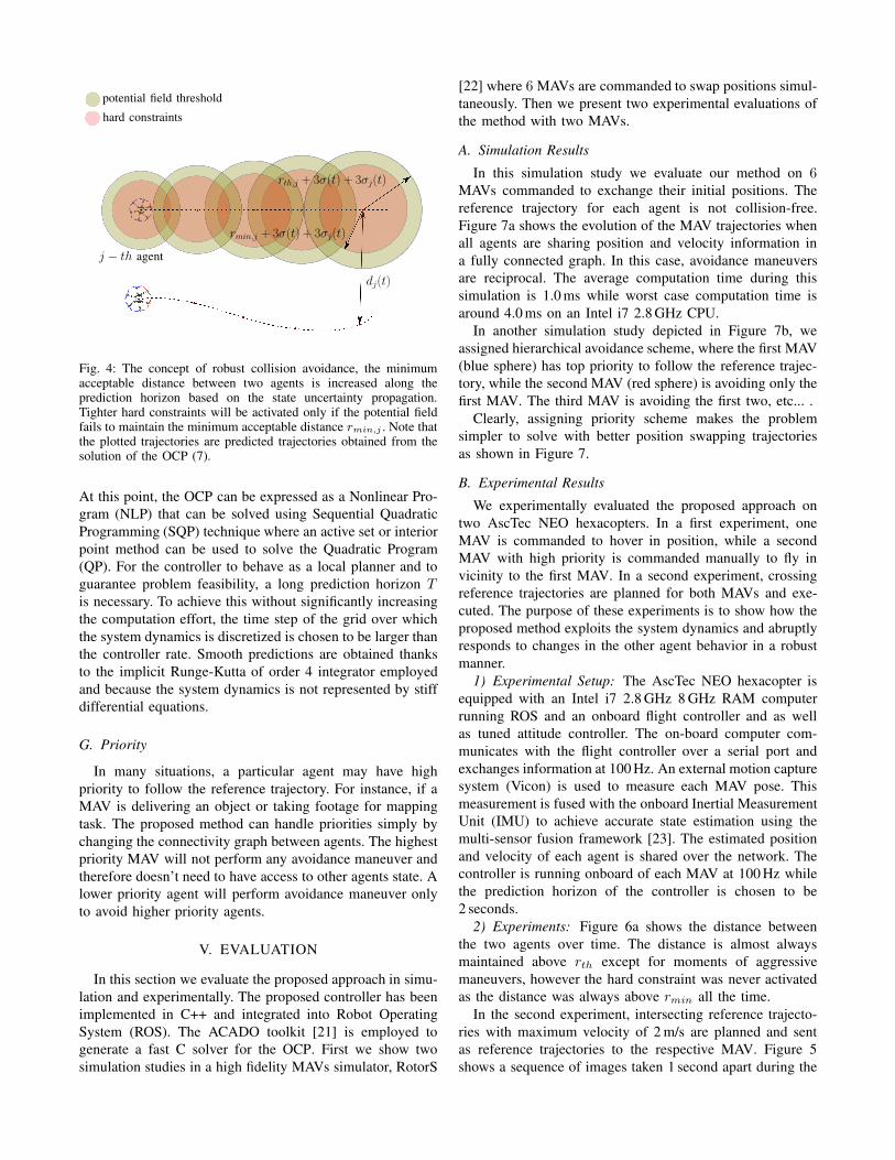
j − th agent

dj(t)

rmin,j + 3σ(t) + 3σj(t)

potential field threshold

hard constraints

rth,j + 3σ(t) + 3σj(t)

Fig. 4: The concept of robust collision avoidance, the minimumacceptable distance between two agents is increased along theprediction horizon based on the state uncertainty propagation.Tighter hard constraints will be activated only if the potential fieldfails to maintain the minimum acceptable distance rmin,j . Note thatthe plotted trajectories are predicted trajectories obtained from thesolution of the OCP (7).

At this point, the OCP can be expressed as a Nonlinear Pro-

gram (NLP) that can be solved using Sequential Quadratic

Programming (SQP) technique where an active set or interior

point method can be used to solve the Quadratic Program

(QP). For the controller to behave as a local planner and to

guarantee problem feasibility, a long prediction horizon Tis necessary. To achieve this without significantly increasing

the computation effort, the time step of the grid over which

the system dynamics is discretized is chosen to be larger than

the controller rate. Smooth predictions are obtained thanks

to the implicit Runge-Kutta of order 4 integrator employed

and because the system dynamics is not represented by stiff

differential equations.

G. Priority

In many situations, a particular agent may have high

priority to follow the reference trajectory. For instance, if a

MAV is delivering an object or taking footage for mapping

task. The proposed method can handle priorities simply by

changing the connectivity graph between agents. The highest

priority MAV will not perform any avoidance maneuver and

therefore doesn’t need to have access to other agents state. A

lower priority agent will perform avoidance maneuver only

to avoid higher priority agents.

V. EVALUATION

In this section we evaluate the proposed approach in simu-

lation and experimentally. The proposed controller has been

implemented in C++ and integrated into Robot Operating

System (ROS). The ACADO toolkit [21] is employed to

generate a fast C solver for the OCP. First we show two

simulation studies in a high fidelity MAVs simulator, RotorS

[22] where 6 MAVs are commanded to swap positions simul-

taneously. Then we present two experimental evaluations of

the method with two MAVs.

A. Simulation Results

In this simulation study we evaluate our method on 6MAVs commanded to exchange their initial positions. The

reference trajectory for each agent is not collision-free.

Figure 7a shows the evolution of the MAV trajectories when

all agents are sharing position and velocity information in

a fully connected graph. In this case, avoidance maneuvers

are reciprocal. The average computation time during this

simulation is 1.0 ms while worst case computation time is

around 4.0 ms on an Intel i7 2.8 GHz CPU.

In another simulation study depicted in Figure 7b, we

assigned hierarchical avoidance scheme, where the first MAV

(blue sphere) has top priority to follow the reference trajec-

tory, while the second MAV (red sphere) is avoiding only the

first MAV. The third MAV is avoiding the first two, etc... .

Clearly, assigning priority scheme makes the problem

simpler to solve with better position swapping trajectories

as shown in Figure 7.

B. Experimental Results

We experimentally evaluated the proposed approach on

two AscTec NEO hexacopters. In a first experiment, one

MAV is commanded to hover in position, while a second

MAV with high priority is commanded manually to fly in

vicinity to the first MAV. In a second experiment, crossing

reference trajectories are planned for both MAVs and exe-

cuted. The purpose of these experiments is to show how the

proposed method exploits the system dynamics and abruptly

responds to changes in the other agent behavior in a robust

manner.

1) Experimental Setup: The AscTec NEO hexacopter is

equipped with an Intel i7 2.8 GHz 8 GHz RAM computer

running ROS and an onboard flight controller and as well

as tuned attitude controller. The on-board computer com-

municates with the flight controller over a serial port and

exchanges information at 100 Hz. An external motion capture

system (Vicon) is used to measure each MAV pose. This

measurement is fused with the onboard Inertial Measurement

Unit (IMU) to achieve accurate state estimation using the

multi-sensor fusion framework [23]. The estimated position

and velocity of each agent is shared over the network. The

controller is running onboard of each MAV at 100 Hz while

the prediction horizon of the controller is chosen to be

2 seconds.

2) Experiments: Figure 6a shows the distance between

the two agents over time. The distance is almost always

maintained above rth except for moments of aggressive

maneuvers, however the hard constraint was never activated

as the distance was always above rmin all the time.

In the second experiment, intersecting reference trajecto-

ries with maximum velocity of 2 m/s are planned and sent

as reference trajectories to the respective MAV. Figure 5

shows a sequence of images taken 1 second apart during the

experiment 1. Figure 6b shows the distance between the two

MAVs over time. The hard constraint was never active since

the distance was always above rmin.

VI. CONCLUSIONS

In this paper we presented a multi-MAVs collision avoid-

ance strategy based on Nonlinear Model Predictive Control.

The approach accounts for state estimator uncertainty by

propagating the uncertainty along the prediction horizon to

increase the minimum acceptable distance between agents,

providing robust collision avoidance. Tight hard constraints

on the distance between agents guarantee no collisions if

the prediction horizon is sufficiently long. Moreover, by

changing the connectivity graph, it is possible to assign

priority to certain agents to follow their reference trajectories.

The approach has been evaluated in simulation with 6 agents

and in real experiments with 2 agents. Our experiments

showed that this collision avoidance approach results into

agile and dynamic avoidance maneuvers while maintaining

system stability at reasonable computational cost.

ACKNOWLEDGMENT

This work was supported by the European Union’s Hori-

zon 2020 Research and Innovation Programme under the

Grant Agreement No.644128, AEROWORKS.

REFERENCES

[1] K. Steich, M. Kamel, P. Beardsleys, M. K. Obrist, R. Siegwart,and T. Lachat, “Tree cavity inspection using aerial robots,” in 2016

IEEE/RSJ International Conference on Intelligent Robots and Systems

(IROS), October 2016.

[2] A. Bircher, M. Kamel, K. Alexis, H. Oleynikova, and R. Siegwart,“Receding horizon ”next-best-view” planner for 3d exploration,” in2016 IEEE International Conference on Robotics and Automation

(ICRA), May 2016, pp. 1462–1468.

[3] A. Girard, A. Howell, and J. Hedrick, “Border patrol and surveillancemissions using multiple unmanned air vehicles,” in Decision and

Control, 2004. CDC. 43rd IEEE Conference on, 2004.

[4] P. Oettershagen, T. J. Stastny, T. A. Mantel, A. S. Melzer, K. Rudin,G. Agamennoni, K. Alexis, R. Siegwart, “Long-endurance sensing andmapping using a hand-launchable solar-powered uav,” in Field and

Service Robotics, 10th Conference on, June 2015, (accepted).

[5] E. R. Hunt, W. D. Hively, S. J. Fujikawa, D. S. Linden, C. S. T.Daughtry, and G. W. McCarty, “Acquisition of nir-green-blue digitalphotographs from unmanned aircraft for crop monitoring,” Remote

Sensing, vol. 2, no. 1, pp. 290–305, 2010.

[6] P. Rudol and P. Doherty, “Human body detection and geolocalizationfor uav search and rescue missions using color and thermal imagery,”in Aerospace Conference, 2008 IEEE, 2008, pp. 1–8.

[7] N. Michael, D. Mellinger, Q. Lindsey, and V. Kumar, “The graspmultiple micro-uav testbed,” IEEE Robotics & Automation Magazine,vol. 17, no. 3, pp. 56–65, 2010.

[8] M. Burri, H. Oleynikova, M. W. Achtelik, and R. Siegwart, “Real-timevisual-inertial mapping, re-localization and planning onboard mavs inunknown environments,” in Intelligent Robots and Systems (IROS),

2015 IEEE/RSJ International Conference on. IEEE, 2015, pp. 1872–1878.

[9] E. Frazzoli, M. A. Dahleh, and E. Feron, “Real-time motion planningfor agile autonomous vehicles,” Journal of Guidance, Control, and

Dynamics, vol. 25, no. 1, pp. 116–129, 2002.

[10] A. Kushleyev, D. Mellinger, C. Powers, and V. Kumar, “Towards aswarm of agile micro quadrotors,” Autonomous Robots, vol. 35, no. 4,pp. 287–300, 2013.

1video available on http://goo.gl/RWRhmJ

[11] F. Augugliaro, A. P. Schoellig, and R. D’Andrea, “Generation ofcollision-free trajectories for a quadrocopter fleet: A sequential convexprogramming approach,” in Intelligent Robots and Systems (IROS),

2012 IEEE/RSJ International Conference on. IEEE, 2012, pp. 1917–1922.

[12] D. H. Shim, H. J. Kim, and S. Sastry, “Decentralized nonlinear modelpredictive control of multiple flying robots,” in Decision and control,

2003. Proceedings. 42nd IEEE conference on, vol. 4. IEEE, 2003,pp. 3621–3626.

[13] J. Alonso-Mora, T. Naegeli, R. Siegwart, and P. Beardsley, “Collisionavoidance for aerial vehicles in multi-agent scenarios,” Autonomous

Robots, vol. 39, no. 1, pp. 101–121, 2015.[14] M. Neunert, C. de Crousaz, F. Furrer, M. Kamel, F. Farshidian,

R. Siegwart, and J. Buchli, “Fast nonlinear model predictive controlfor unified trajectory optimization and tracking,” in Robotics and

Automation (ICRA), 2016 IEEE International Conference on. IEEE,2016, pp. 1398–1404.

[15] R. Mahony, V. Kumar, and P. Corke, “Multirotor aerial vehicles: Mod-eling, estimation, and control of quadrotor,” IEEE Robotics Automation

Magazine, vol. 19, no. 3, pp. 20–32, Sept 2012.[16] S. Omari, M. D. Hua, G. Ducard, and T. Hamel, “Nonlinear control

of vtol uavs incorporating flapping dynamics,” in 2013 IEEE/RSJ

International Conference on Intelligent Robots and Systems, Nov2013, pp. 2419–2425.

[17] M. Burri, J. Nikolic, H. Oleynikova, M. W. Achtelik, and R. Siegwart,“Maximum likelihood parameter identification for mavs,” in 2016

IEEE International Conference on Robotics and Automation (ICRA),May 2016, pp. 4297–4303.

[18] M. Blosch, S. Weiss, D. Scaramuzza, and R. Siegwart, “Visionbased mav navigation in unknown and unstructured environments,” inRobotics and automation (ICRA), 2010 IEEE international conference

on. IEEE, 2010, pp. 21–28.[19] M. Kamel, T. Stastny, K. Alexis, and R. Siegwart”, “”model predictive

control for trajectory tracking of unmanned aerial vehicles using robotoperating system”,” in ”Robot Operating System (ROS) The Complete

Reference”, A. Koubaa”, Ed. ”Springer Press”, “2017”, ”(to appear)”.[20] C. Kirches, The Direct Multiple Shooting Method for Optimal

Control. Wiesbaden: Vieweg+Teubner Verlag, 2011, pp. 13–29.[Online]. Available: http://dx.doi.org/10.1007/978-3-8348-8202-8 2

[21] B. Houska, H. Ferreau, and M. Diehl, “ACADO Toolkit – An OpenSource Framework for Automatic Control and Dynamic Optimization,”Optimal Control Applications and Methods, vol. 32, no. 3, pp. 298–312, 2011.

[22] F. Furrer, M. Burri, M. Achtelik, and R. Siegwart, Robot Operating

System (ROS): The Complete Reference (Volume 1). Cham: SpringerInternational Publishing, 2016, ch. RotorS—A Modular GazeboMAV Simulator Framework, pp. 595–625. [Online]. Available:http://dx.doi.org/10.1007/978-3-319-26054-9 23

[23] S. Lynen, M. W. Achtelik, S. Weiss, M. Chli, and R. Siegwart,“A robust and modular multi-sensor fusion approach applied to mavnavigation,” in Intelligent Robots and Systems (IROS), 2013 IEEE/RSJ

International Conference on. IEEE, 2013, pp. 3923–3929.

Fig. 5: A sequence of images during the cross trajectories experiments. The two MAVs are commanded to follow a non collision-freetrajectories with priority assigned to the MAV with the red hat. Images are taken 1 second apart starting from top left.

20 40 60 80 100 120 140 160

time [sec]

0

1

2

3

4

dis

tance [m

]

Manual flight experiment

distance between MAVs

rmin

rth

0 0.5 1 1.5 2 2.5 3

distance [m]

0

500

1000

1500

2000

2500

3000

co

unt

Histogram of MAVs distance

(a) The upper plot shows the distance between two MAVsover time during the manual flight experiment. One MAV iscommanded to hover in position while the other one is manuallycommanded to approach it with a priority assigned to themanually commanded MAV. rth is set to 1.2 m while the hardconstraint on the distance is set to rmin = 0.9 m. The lowerplot shows the histogram of the distance.

10 20 30 40 50 60

time [sec]

0

1

2

3

4

dis

tance [m

]

Cross reference trajectory flight experiment

distance between MAVs

rmin

rth

0 0.5 1 1.5 2 2.5 3 3.5

distance [m]

0

200

400

600

800

1000

1200

1400

co

unt

Histogram of MAVs distance

(b) The upper plot shows the distance between two MAVs overtime during the crossing trajectories experiment. rth is set to1.2 m while the hard constraint on the distance is set to rmin =0.9 m. The lower plot shows the histogram of the distance.

Fig. 6: Experimental results with two MAVs

(a) Trajectories of 6 MAVs during a position swapping simulation. The MAVs are represented by spheres, while dotted lines representthe reference trajectory provided to the controller. Solid lines represent the actual trajectory executed by each agent.

(b) Trajectories of 6 MAVs during a position swapping simulation with priority given to the first MAV (blue sphere). Dotted linesrepresent the reference trajectory provided to the controller. Solid lines represent the actual trajectory executed by each agent.

Fig. 7: Simulation results of 6 MAVs exchanging positions