Nonlinear Least-Squares Problems with the Gauss … Least-Squares Problems with the Gauss-Newton and...

Nonlinear Least-Squares Problems with theGauss-Newton and Levenberg-Marquardt

Methods

Alfonso Croeze1 Lindsey Pittman2 Winnie Reynolds1

1Department of MathematicsLouisiana State University

Baton Rouge, LA

2Department of MathematicsUniversity of Mississippi

Oxford, MS

July 6, 2012

Croeze, Pittman, Reynolds LSU&UoM

The Gauss-Newton and Levenberg-Marquardt Methods

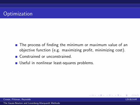
Optimization

The process of finding the minimum or maximum value of anobjective function (e.g. maximizing profit, minimizing cost).

Constrained or unconstrained.

Useful in nonlinear least-squares problems.



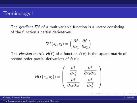
Terminology I

The gradient ∇f of a multivariable function is a vector consistingof the function’s partial derivatives:

∇f (x1, x2) =

(∂f

∂x1,∂f

∂x2

)The Hessian matrix H(f ) of a function f (x) is the square matrix ofsecond-order partial derivatives of f (x):

H(f (x1, x2)) =

∂f

∂x21

∂f

∂x1∂x2

∂f

∂x1∂x2

∂f

∂x22



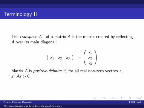
Terminology II

The transpose A> of a matrix A is the matrix created by reflectingA over its main diagonal:

(x1 x2 x3

)>=

x1x2x3

Matrix A is positive-definite if, for all real non-zero vectors z ,z>Az > 0.



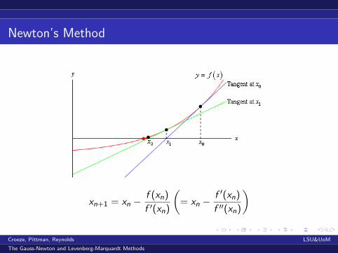
Newton’s Method

xn+1 = xn −f (xn)

f ′(xn)

(= xn −

f ′(xn)

f ′′(xn)

)



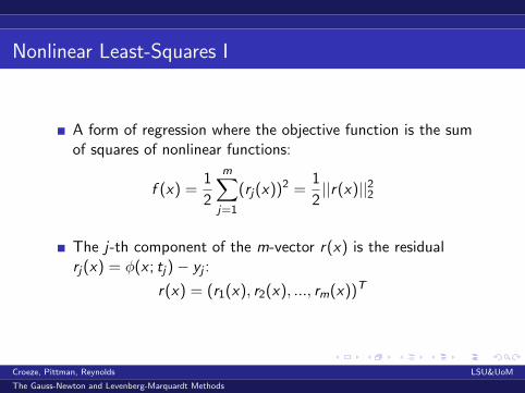
Nonlinear Least-Squares I

A form of regression where the objective function is the sumof squares of nonlinear functions:

f (x) =1

2

m∑j=1

(rj(x))2 =1

2||r(x)||22

The j-th component of the m-vector r(x) is the residualrj(x) = φ(x ; tj)− yj :

r(x) = (r1(x), r2(x), ..., rm(x))T



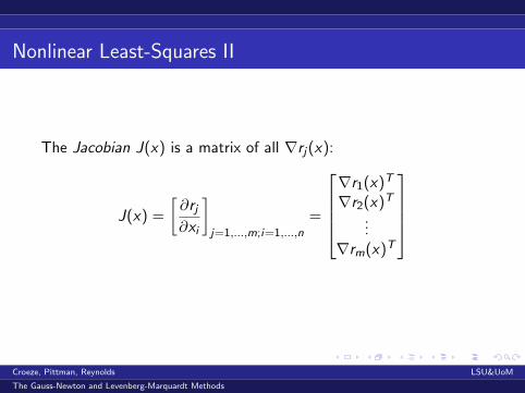
Nonlinear Least-Squares II

The Jacobian J(x) is a matrix of all ∇rj(x):

J(x) =

[∂rj∂xi

]j=1,...,m;i=1,...,n

=

∇r1(x)T

∇r2(x)T

...∇rm(x)T



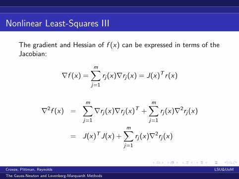
Nonlinear Least-Squares III

The gradient and Hessian of f (x) can be expressed in terms of theJacobian:

∇f (x) =m∑j=1

rj(x)∇rj(x) = J(x)T r(x)

∇2f (x) =m∑j=1

∇rj(x)∇rj(x)T +m∑j=1

rj(x)∇2rj(x)

= J(x)T J(x) +m∑j=1

rj(x)∇2rj(x)



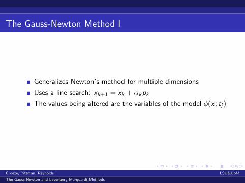
The Gauss-Newton Method I

Generalizes Newton’s method for multiple dimensions

Uses a line search: xk+1 = xk + αkpk

The values being altered are the variables of the model φ(x ; tj)



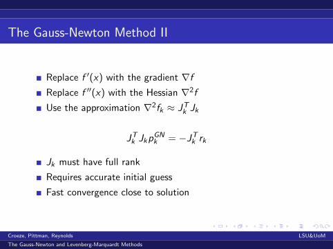
The Gauss-Newton Method II

Replace f ′(x) with the gradient ∇f

Replace f ′′(x) with the Hessian ∇2f

Use the approximation ∇2fk ≈ JTk Jk

JTk JkpGN

k = −JTk rk

Jk must have full rank

Requires accurate initial guess

Fast convergence close to solution



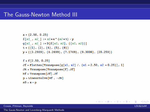
The Gauss-Newton Method III



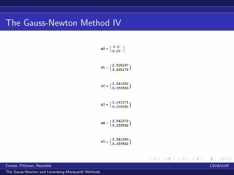
The Gauss-Newton Method IV



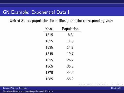
GN Example: Exponential Data I

United States population (in millions) and the corresponding year:

Year Population

1815 8.3

1825 11.0

1835 14.7

1845 19.7

1855 26.7

1865 35.2

1875 44.4

1885 55.9



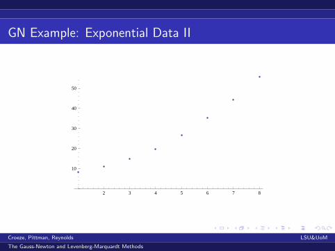
GN Example: Exponential Data II

2 3 4 5 6 7 8

10

20

30

40

50



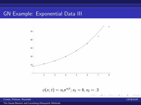
GN Example: Exponential Data III

2 3 4 5 6 7 8

10

20

30

40

50

φ(x ; t) = x1ex2t ; x1 = 6, x2 = .3



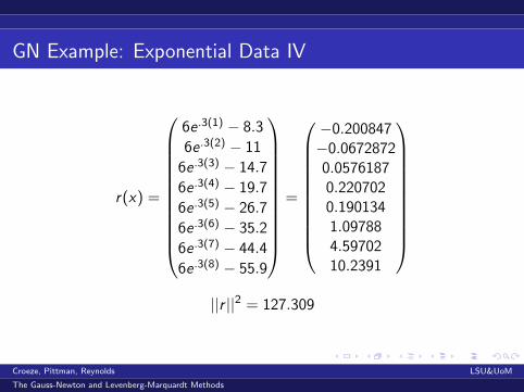
GN Example: Exponential Data IV

r(x) =

6e .3(1) − 8.3

6e .3(2) − 11

6e .3(3) − 14.7

6e .3(4) − 19.7

6e .3(5) − 26.7

6e .3(6) − 35.2

6e .3(7) − 44.4

6e .3(8) − 55.9

=

−0.200847−0.06728720.05761870.2207020.1901341.097884.5970210.2391

||r ||2 = 127.309



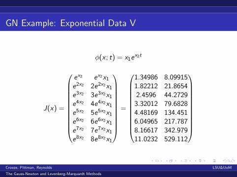
GN Example: Exponential Data V

φ(x ; t) = x1ex2t

J(x) =

ex2 ex2x1e2x2 2e2x2x1e3x2 3e3x2x1e4x2 4e4x2x1e5x2 5e5x2x1e6x2 6e6x2x1e7x2 7e7x2x1e8x2 8e8x2x1

=

1.34986 8.099151.82212 21.86542.4596 44.2729

3.32012 79.68284.48169 134.4516.04965 217.7878.16617 342.97911.0232 529.112



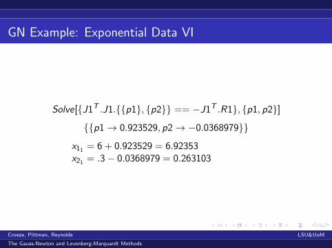
GN Example: Exponential Data VI

Solve[{J1T .J1.{{p1}, {p2}} == −J1T .R1}, {p1, p2}]

{{p1→ 0.923529, p2→ −0.0368979}}

x11 = 6 + 0.923529 = 6.92353x21 = .3− 0.0368979 = 0.263103



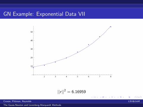
GN Example: Exponential Data VII

2 3 4 5 6 7 8

10

20

30

40

50

||r ||2 = 6.16959



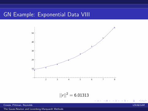
GN Example: Exponential Data VIII

2 3 4 5 6 7 8

10

20

30

40

50

||r ||2 = 6.01313



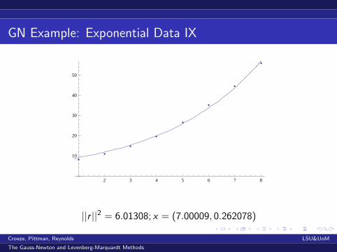
GN Example: Exponential Data IX

2 3 4 5 6 7 8

10

20

30

40

50

||r ||2 = 6.01308; x = (7.00009, 0.262078)



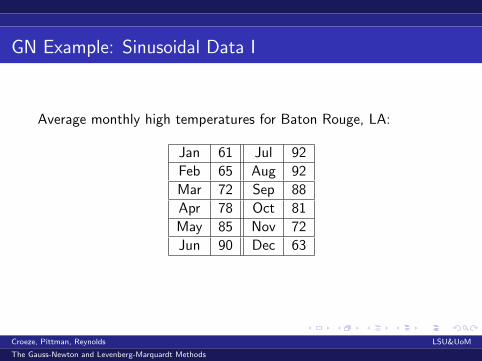
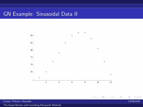
GN Example: Sinusoidal Data I

Average monthly high temperatures for Baton Rouge, LA:

Jan 61 Jul 92

Feb 65 Aug 92

Mar 72 Sep 88

Apr 78 Oct 81

May 85 Nov 72

Jun 90 Dec 63



GN Example: Sinusoidal Data II

2 4 6 8 10 12

65

70

75

80

85

90



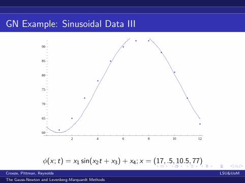
GN Example: Sinusoidal Data III

2 4 6 8 10 12

60

65

70

75

80

85

90

φ(x ; t) = x1 sin(x2t + x3) + x4; x = (17, .5, 10.5, 77)



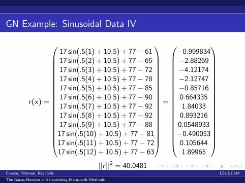
GN Example: Sinusoidal Data IV

r(x) =

17 sin(.5(1) + 10.5) + 77− 6117 sin(.5(2) + 10.5) + 77− 6517 sin(.5(3) + 10.5) + 77− 7217 sin(.5(4) + 10.5) + 77− 7817 sin(.5(5) + 10.5) + 77− 8517 sin(.5(6) + 10.5) + 77− 9017 sin(.5(7) + 10.5) + 77− 9217 sin(.5(8) + 10.5) + 77− 9217 sin(.5(9) + 10.5) + 77− 88

17 sin(.5(10) + 10.5) + 77− 8117 sin(.5(11) + 10.5) + 77− 7217 sin(.5(12) + 10.5) + 77− 63

=

−0.999834−2.88269−4.12174−2.12747−0.857160.6643351.84033

0.8932160.0548933−0.4900530.1056441.89965

||r ||2 = 40.0481



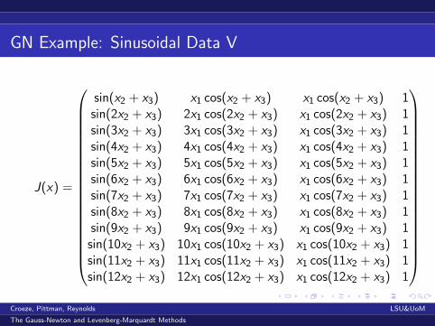
GN Example: Sinusoidal Data V

J(x) =

sin(x2 + x3) x1 cos(x2 + x3) x1 cos(x2 + x3) 1sin(2x2 + x3) 2x1 cos(2x2 + x3) x1 cos(2x2 + x3) 1sin(3x2 + x3) 3x1 cos(3x2 + x3) x1 cos(3x2 + x3) 1sin(4x2 + x3) 4x1 cos(4x2 + x3) x1 cos(4x2 + x3) 1sin(5x2 + x3) 5x1 cos(5x2 + x3) x1 cos(5x2 + x3) 1sin(6x2 + x3) 6x1 cos(6x2 + x3) x1 cos(6x2 + x3) 1sin(7x2 + x3) 7x1 cos(7x2 + x3) x1 cos(7x2 + x3) 1sin(8x2 + x3) 8x1 cos(8x2 + x3) x1 cos(8x2 + x3) 1sin(9x2 + x3) 9x1 cos(9x2 + x3) x1 cos(9x2 + x3) 1

sin(10x2 + x3) 10x1 cos(10x2 + x3) x1 cos(10x2 + x3) 1sin(11x2 + x3) 11x1 cos(11x2 + x3) x1 cos(11x2 + x3) 1sin(12x2 + x3) 12x1 cos(12x2 + x3) x1 cos(12x2 + x3) 1



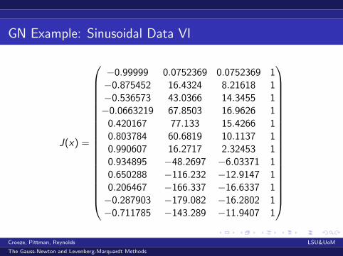
GN Example: Sinusoidal Data VI

J(x) =

−0.99999 0.0752369 0.0752369 1−0.875452 16.4324 8.21618 1−0.536573 43.0366 14.3455 1−0.0663219 67.8503 16.9626 1

0.420167 77.133 15.4266 10.803784 60.6819 10.1137 10.990607 16.2717 2.32453 10.934895 −48.2697 −6.03371 10.650288 −116.232 −12.9147 10.206467 −166.337 −16.6337 1−0.287903 −179.082 −16.2802 1−0.711785 −143.289 −11.9407 1



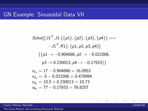
GN Example: Sinusoidal Data VII

Solve[{J1T .J1.{{p1}, {p2}, {p3}, {p4}} ==

−J1T .R1}, {p1, p2, p3, p4}]

{{p1→ −0.904686, p2→ −0.021006,

p3→ 0.230013, p4→ −0.17933}}

x11 = 17− 0.904686 = 16.0953x21 = .5− 0.021006 = 0.478994x31 = 10.5 + 0.230013 = 10.73x41 = 77− 0.17933 = 76.8207



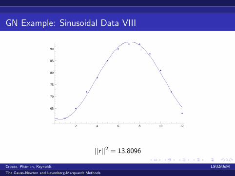
GN Example: Sinusoidal Data VIII

2 4 6 8 10 12

65

70

75

80

85

90

||r ||2 = 13.8096



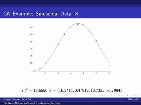
GN Example: Sinusoidal Data IX

2 4 6 8 10 12

65

70

75

80

85

90

||r ||2 = 13.6556; x = (16.2411, 0.47912, 10.7335, 76.7994)



Gradient Descent

xk+1 = xk − λk∇f (xk)

Quickly approaches the solution from a distance.

Convergence becomes very slow close to the solution.



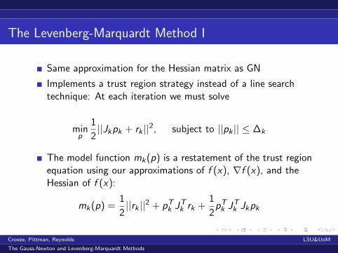
The Levenberg-Marquardt Method I

Same approximation for the Hessian matrix as GN

Implements a trust region strategy instead of a line searchtechnique: At each iteration we must solve

minp

1

2||Jkpk + rk ||2, subject to ||pk || ≤ ∆k

The model function mk(p) is a restatement of the trust regionequation using our approximations of f (x), ∇f (x), and theHessian of f (x):

mk(p) =1

2||rk ||2 + pT

k JTk rk +

1

2pTk JT

k Jkpk



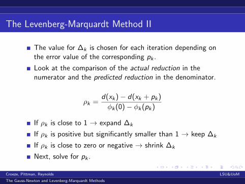
The Levenberg-Marquardt Method II

The value for ∆k is chosen for each iteration depending onthe error value of the corresponding pk .

Look at the comparison of the actual reduction in thenumerator and the predicted reduction in the denominator.

ρk =d(xk)− d(xk + pk)

φk(0)− φk(pk)

If ρk is close to 1 → expand ∆k

If ρk is positive but significantly smaller than 1 → keep ∆k

If ρk is close to zero or negative → shrink ∆k

Next, solve for pk .



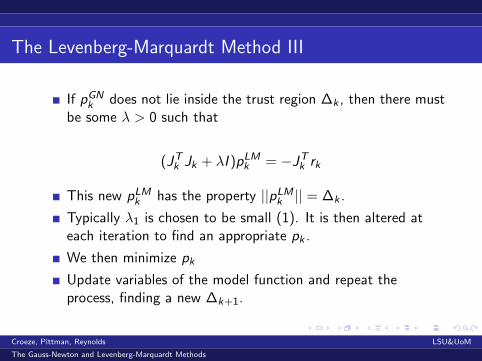
The Levenberg-Marquardt Method III

If pGNk does not lie inside the trust region ∆k , then there must

be some λ > 0 such that

(JTk Jk + λI )pLM

k = −JTk rk

This new pLMk has the property ||pLM

k || = ∆k .

Typically λ1 is chosen to be small (1). It is then altered ateach iteration to find an appropriate pk .

We then minimize pk

Update variables of the model function and repeat theprocess, finding a new ∆k+1.



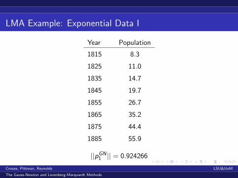
LMA Example: Exponential Data I

Year Population

1815 8.3

1825 11.0

1835 14.7

1845 19.7

1855 26.7

1865 35.2

1875 44.4

1885 55.9

||pGN1 || = 0.924266



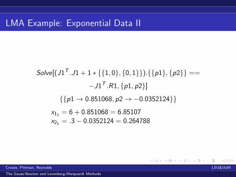
LMA Example: Exponential Data II

Solve[(J1T .J1 + 1 ∗ {{1, 0}, {0, 1}}).{{p1}, {p2}} ==

−J1T .R1, {p1, p2}]

{{p1→ 0.851068, p2→ −0.0352124}}

x11 = 6 + 0.851068 = 6.85107x21 = .3− 0.0352124 = 0.264788



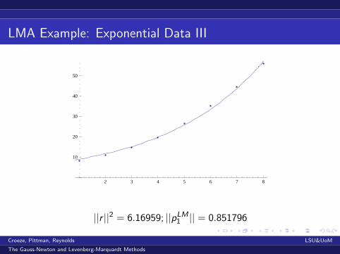
LMA Example: Exponential Data III

2 3 4 5 6 7 8

10

20

30

40

50

||r ||2 = 6.16959; ||pLM1 || = 0.851796



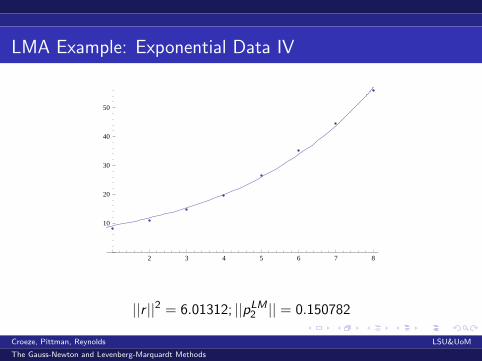
LMA Example: Exponential Data IV

2 3 4 5 6 7 8

10

20

30

40

50

||r ||2 = 6.01312; ||pLM2 || = 0.150782



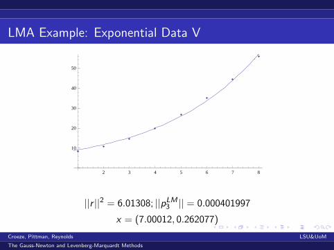
LMA Example: Exponential Data V

2 3 4 5 6 7 8

10

20

30

40

50

||r ||2 = 6.01308; ||pLM3 || = 0.000401997

x = (7.00012, 0.262077)



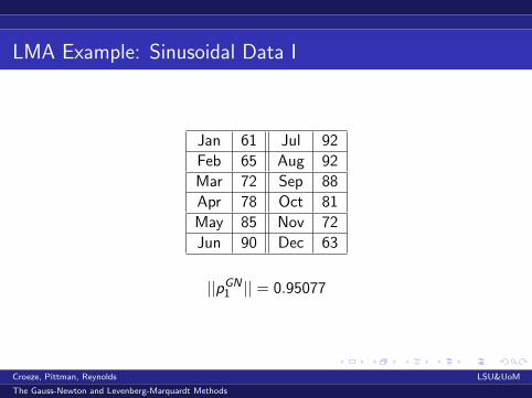
LMA Example: Sinusoidal Data I

Jan 61 Jul 92

Feb 65 Aug 92

Mar 72 Sep 88

Apr 78 Oct 81

May 85 Nov 72

Jun 90 Dec 63

||pGN1 || = 0.95077



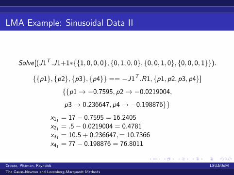
LMA Example: Sinusoidal Data II

Solve[(J1T .J1+1∗{{1, 0, 0, 0}, {0, 1, 0, 0}, {0, 0, 1, 0}, {0, 0, 0, 1}}).

{{p1}, {p2}, {p3}, {p4}} == −J1T .R1, {p1, p2, p3, p4}]

{{p1→ −0.7595, p2→ −0.0219004,

p3→ 0.236647, p4→ −0.198876}}

x11 = 17− 0.7595 = 16.2405x21 = .5− 0.0219004 = 0.4781x31 = 10.5 + 0.236647,= 10.7366x41 = 77− 0.198876 = 76.8011



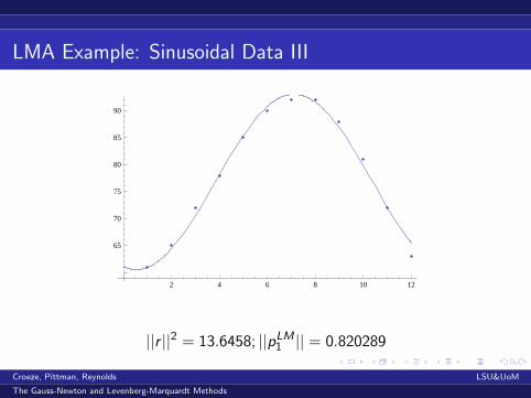
LMA Example: Sinusoidal Data III

2 4 6 8 10 12

65

70

75

80

85

90

||r ||2 = 13.6458; ||pLM1 || = 0.820289



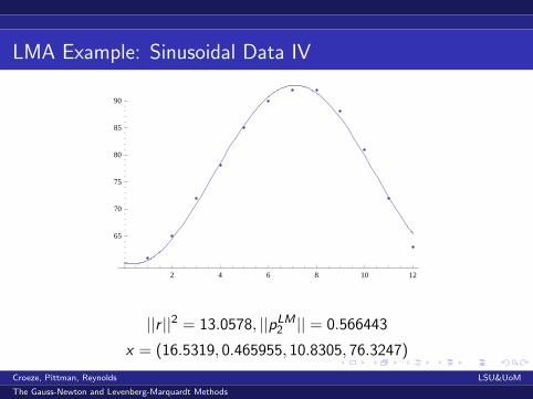
LMA Example: Sinusoidal Data IV

2 4 6 8 10 12

65

70

75

80

85

90

||r ||2 = 13.0578, ||pLM2 || = 0.566443

x = (16.5319, 0.465955, 10.8305, 76.3247)



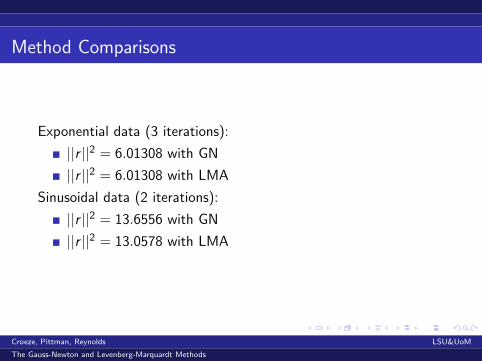
Method Comparisons

Exponential data (3 iterations):

||r ||2 = 6.01308 with GN

||r ||2 = 6.01308 with LMA

Sinusoidal data (2 iterations):

||r ||2 = 13.6556 with GN

||r ||2 = 13.0578 with LMA



Limitations

Both GN and LMA approximate ∇2f (x) by eliminating thesecond term involving ∇2r .

If the residual is large or the model does not fit the functionwell, other methods must be used.

Local minimum vs. global minimum



Bibliography I

”Average Weather for Baton Rouge, LA - Temperature andPrecipitation.” The Weather Channel. 28 June 2012(http://www.weather.com/weather/wxclimatology/monthly/graph/USLA0033)

Gill, Philip E.; Murray, Walter. Algorithms for the solution ofthe nonlinear least-squares problem. SIAM Journal onNumerical Analysis 15 (5): 977-992. 1978.

Griva, Igor; Nash, Stephen; Sofer Ariela. Linear and NonlinearOptimization. 2nd ed. Society for Industrial Mathematics.2008.

Nocedal, Jorge; Wright, Steven J. Numerical Optimization,2nd Edition. Springer, Berlin, 2006.



Bibliography II

”The Population of the United States.” University of Illinois.28 June 2012 (mste.illinois.edu/malcz/ExpFit/data.html).

Ranganathan, Ananth. ”The Levenberg-MarquardtAlgorithm.” Honda Research Institute, USA. 8 June 2004. 1July 2012 (http://ananth.in/Notes files/lmtut.pdf).



Acknowledgements

Dr. Mark Davidson

Dr. Humberto Munoz

Ladorian Latin



Nonlinear Least-Squares Problems with the Gauss … Least-Squares Problems with the Gauss-Newton and...

Documents

Transcript of Nonlinear Least-Squares Problems with the Gauss … Least-Squares Problems with the Gauss-Newton and...