NONLINEAR COMPUTATIONAL SOLID & …...NONLINEAR COMPUTATIONAL SOLID & STRUCTURAL MECHANICS...

NONLINEAR COMPUTATIONALSOLID & STRUCTURAL MECHANICS

Theoretical formulations, technologies and computationsPavia, May 5–9, 2014

Lecture 8. May 6, 2014

Inelastic constitutive behavior

at small strains

Ferdinando Auricchio

e-mail: [email protected]: http://www.unipv.it/compmech

F.Auricchio (UNIPV – IMATI) Computational inelasticity 1 / 70

Lecture goal

Lecture 8. Inelastic constitutive behavior

Inelasticity and plasticity models

Solution schemes (return map)

Integration of evolution equations

Operator split method and consistent tangent modulus

F.Auricchio (UNIPV – IMATI) Computational inelasticity January 8, 2015 2 / 70

Motivations

Perform a standard traction test ... for cyclic loading-loading

⋆ Distinguish between reversible (elastic) and irreversible (inelastic region)

⋆ Threshold stress limit between the two regions

⋆ Complex response under cyclic loading ( ... up to fatigue!)

Question: how is it possible to model such effects and compute with them


Overview I

General format for inelasticity as evolutionary models

Linear visco-elasticity

Visco-plasticity

J2 plasticity

More general plasticity models

Integration algorithm

Solution algorithm

⋆ Load conditions depend on time t

⋆ Dependence on time t not explicitly stated

⋆ Small deformation regime


Introduction: elastic vs inelastic I

Elastic material: stress is function only of strain, or, equivalentlyin case of no internal constraint, strain is function only of stress

εεε = εεε(σ)

Elastic material ⇒ constitutive response independentfrom process followed in reaching actual state

Elastic assumption is clearly an approximation of real material behavior, very close insome cases, rough in other cases

Thinking of strain as dependent variable, strain may depend not only on stress atcurrent time, but also on stress path followed to reach current state


Introduction: elastic vs inelastic IIWhenever path dependence is significant, material must be regarded as inelastic

Inelastic material: strain is function not only of stress, but alsoof other quantities, in general, indicated as internal variables, ξ

εεε = εεε(σ, ξ)

Internal variables ξ: a set of scalars, tensors, or whatever needed to properlydescribe material response

Since ξ are new variables, need to introduce extra equations, internal variableconstitutive equations, for example, in rate form (!)

ξ = g(σ, ξ)

i.e., through differential equations that determine rates in time (time derivatives)

Inelastic material:

εεε = εεε(σ, ξ)

ξ = g(σ, ξ)

Note: all quantities assumed to be function of time t: εεε = εεε(t), σ = σ(t), ξ = ξ(t)

Distinguish between external or control variables (εεε,σ) and internal variables (ξ)

Two equations in three unknowns: select independent control variable


Introduction: elastic vs inelastic III

Within small deformations, additive decomposition of strain

εεε = εεεe + εεε

i

where: εεεe : elastic strain, i.e. part of strain related to stress

through elastic relation or part of strain function onlyof stress, i.e. εεεe = εεεe(σ)

εεεi : inelastic strain, i.e. difference between total andelastic strain, i.e. εεεi = εεε− εεεe

Assume inelastic strain εεεi as internal variable

ξ = εεεi ⇒

εεε = εεε(σ,εεεi )

εεεi = g(σ,εεεi )

ξ = εεεi,β ⇒

εεε = εεε(σ,εεεi ,β)

εεεi = g1(σ,εεε

i,β)

β = g2(σ,εεεi,β)


Notation I

Split stress, σ, and strain, εεε, in deviatoric and volumetric components

σ = s+ pI

εεε = e +1

3θI

with

tr(s) = s : I = 0

tr(e) = e : I = 0and

p =1

3tr(σ) =

1

3σ : I

θ = tr(εεε) = εεε : I

where tr(•) : trace operator I: second rank identity tensor

Deviatoric-volumetric decomposition consistent with additive strain decomposition

εεεe = ee +

1

3θe I

εεεi = ei +

1

3θi I

and

e = ee + ei

θ = θe + θ

i

For any any second rank tensor a introduce Euclidean inner product (trace)

‖a‖ = [a : a]12 = [ tr(a · a) ] 12


Non-linear inelastic constitutive model I

Focus on a simple model

εεε = εεε(σ,εεεi )

εεεi = g(σ,εεεi)

GOAL: compute material model evolution/response under specific/generic loadingconditions (“virtual” experimental test)

Recall: all quantities assumed to be function of time t

Before computing model evolution, need to do several considerationsX Time-continuous setting: non-linear differential-algebraic eqs?? Time-discrete setting: integration in time → non-linear algebraic eqs?? Time-marching algorithm: solve non-linearity → advance in time

( discrete constitutive algorithm )

Start defining time-discrete setting


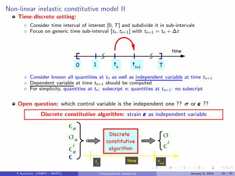
Non-linear inelastic constitutive model IITime-discrete setting:

Consider time interval of interest [0,T ] and subdivide it in sub-intervals Focus on generic time sub-interval [tn, tn+1] with tn+1 = tn +∆t

Consider known all quantities at tn as well as independent variable at time tn+1

Dependent variable at time tn+1 should be computed For simplicity, quantities at tn: subscript n; quantities at tn+1: no subscript

Open question: which control variable is the independent one ?? σ or εεε ??

Discrete constitutive algorithm: strain εεε as independent variable


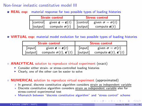
Non-linear inelastic constitutive model III

REAL exp: material response for two possible types of loading histories

Strain control Stress control

[control] given εεε = εεε(t) [control] given σ = σ(t)[output] compute σ(t) [output] compute εεε(t)

VIRTUAL exp: material model evolution for two possible types of loading histories

Strain control Stress control

[input] given εεε = εεε(t) [input] given σ = σ(t)[output] compute σ(t), εεεi (t) [output] compute εεε(t), εεεi(t)

ANALYTICAL solution to reproduce virtual experiment (exact) Consider either strain- or stress-controlled loading histories Clearly, one of the other can be easier to solve

NUMERICAL solution to reproduce virtual experiment (approximated)⋆ In general, discrete constitutive algorithm considers strain as independent variable⋆ Discrete constitutive algorithm considers strain as independent variable also for

stress-control experimental test⋆ Mismatch between “discrete constitutive algorithm” and “stress control” scheme


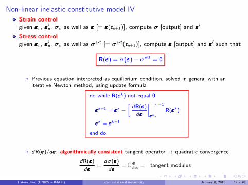
Non-linear inelastic constitutive model IV

Strain controlgiven εεεn, εεε

in, σn as well as εεε [= εεε(tn+1)], compute σ [output] and εεεi

Stress controlgiven εεεn, εεε

in, σn as well as σext [= σext(tn+1)], compute εεε [output] and εεεi such that

R(εεε) = σ(εεε)− σext = 0

Previous equation interpreted as equilibrium condition, solved in general with aniterative Newton method, using update formula

do while R(εεεk) not equal 0

εεεk+1 = εεεk −[

dR(εεε)

dεεε

∣

∣

∣

∣

εεεk

]

−1

R(εεεk)

εεεk = εεεk+1

end do

dR(εεε)/dεεε: algorithmically consistent tangent operator → quadratic convergence

dR(εεε)

dεεε=

dσ(εεε)

dεεε= C

tgdisc = tangent modulus


Non-linear inelastic constitutive model V

Compute fourth-order tangent tensor Ctgdisc, consistent (!!) with time-discrete model

dσ = Ctgdiscdεεε

Necessary in general to solve equilibrium problems

Point-wise (local) equilibrium. Assign a stress history σext(t). To compute strainhistory which produces the assigned stress history, solve equation

R(εεε) = σ(εεε)− σext = 0

where all quantities are assumed to be evaluated at time tn+1

Boundary-value (global) equilibrium. Assign a standard BVP with load and BCsvarying in time. Then at any time tn+1 solve the problem

R = Lint −Lext = 0

where Lint and Lext are respectively internal and external work with

R = Lint(εεε)− Lext =

∫

Ωδεεε : σ(εεε)dV −

∫

Ωδu : bdV = 0

and all field quantities are assumed to be evaluated at time tn+1

Concept of constitutive driver code


Non-linear inelastic constitutive model VI

To solve nonlinear residual equation R(εεε) = 0, often adopted iterative Newtonmethod

START with a tentative solution εεεk

CHECK if tentative solution εεεk is an effective solution, i.e. if R(εεεk) = 0 if YES, then exit If NOT, then UPDATE tentative solution

R(εεεk+1) ≈ 0

i.e.

R(εεεk+1) ≈ R(εεεk)+∂R

∂εεε

∣

∣

∣

∣

εεε=εεεk

(

εεεk+1 − εεεk)

= 0

hence

εεεk+1 = εεεk −[

∂R

∂εεε

]

−1

εεεk

R(εεεk)


Viscoelasticity I

GOAL: develop a model showing inelastic strain evolution and rate-dependency(standard viscoelastic model)

Consider the simplest case: isotropic linear viscoelastic material

Detail model time-continuous and time-discrete version

Due to model linearity, no special algorithm needed for time-discrete approach

Address tangent tensor consistent with discrete model


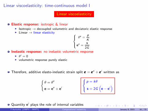
Linear viscoelasticity: time-continuous model I

Linear viscoelasticity

Elastic response: isotropic & linear Isotropic → decoupled volumetric and deviatoric elastic response Linear → linear elasticity

θe =p

K

ee =s

2G

Inelastic response: no inelastic volumetric response θi = 0 volumetric response purely elastic

Therefore, additive elasto-inelastic strain split εεε = εεεe + εεεi written as

θ = θe

e = ee + ei

p = kθ

s = 2G(

e− ei)

Quantity ei plays the role of internal variablesF.Auricchio (UNIPV – IMATI) Computational inelasticity January 8, 2015 16 / 70

Linear viscoelasticity: time-continuous model II

As internal-variable rate-equation, assume simplest linear relation

ei =1

2ηs− 1

λei

with η: material viscosity parameter λ: internal characteristic time

Accordingly, obtain the so-called linear isotropic viscoelastic model

p = Kθ

s = 2G(e− ei )

ei =1

2ηs− 1

λei

Algebraic-differential equations


Linear viscoelasticity: time-discrete counterpart and algorithmic solution I

Goal: develop time discrete counterpart for possible computer implementation

Since model is linear, no special algorithm should be used to obtain the solution

Tangent tensor consistent with discrete model is also addressed

tn and tn+1: two time values

tn+1 > tn and tn+1 first time of interest after tn

Minimize subscript appearance (make equations more readable)

an = a(tn) , a = a(tn+1)

with a any generic quantity

⋆ Quantity evaluated at time tn: subscript n

⋆ Quantity evaluated at time tn+1: no subscript

GOAL: develop a time marching procedure


Linear viscoelasticity: time-discrete counterpart and algorithmic solution II

IDEA: compute stress history from strain history (strain driven problem) Known / given: strain εεε at time tn+1 and solution at time tn

(

σn,εεεn, ein)

Unknown / to be computed: solution at time tn+1

Backward Euler formula to integrate rate equation in time

ei =1

2ηs− 1

λei ⇒ ei − ein

∆t=

1

2ηs− 1

λei

with ∆t = tn+1 − tn

Evaluate remaining equation at tn+1

Continuous-time vs discrete-time model equations

p = Kθ

s = 2G(e− ei )

ei =1

2ηs− 1

λei

⇒

p = Kθ

s = 2G(e− ei )

ei = ein +

[

1

2ηs− 1

λei]

∆t

(1)

Note: no subscript means evaluation at tn+1, e.g., s means s = s(tn+1)


Linear viscoelasticity: time-discrete counterpart and algorithmic solution III

Compute inelastic strain ei update as function of previous solution and current strain(RECALL: strain-driven process)

Combine 12 & 13

ei = α[

ein + βe]

(2)

where:

α =

[

1 +

(

2G

2η+

1

λ

)

∆t

]

−1

, β =2G

2η∆t

Compute stress update using 11 & 12 as well as updated inelastic strain

In conclusion

p = Kθ

ei = α[

ein + βe]

s = 2G(e− ei)


Linear viscoelasticity: time-discrete counterpart and algorithmic solution IV

Algorithmic-consistent tangent tensor Ctgdisc


Linearize deviatoric elastic relation and inelastic strain evolution equation

s = 2G(e− ei )

ei = α[

ein + βe]

⇒

ds = 2G(de− dei )

dei = αβde

Combine previous two relations

ds =[

2G(1− αβ)II]

de

Recalling stress volumetric-deviatoric split, get in compact notation

Ctgdisc = [K(I⊗ I) + 2G(1− αβ)Idev] (3)


Linear viscoelasticity: time-discrete counterpart and algorithmic solution V

Using a matrix notation

Ctgdisc =

[

K(1T1) + 2G(1− αβ)Idev

]

Recall

1 =

111000

, 1T1 =

1 1 1 0 0 01 1 1 0 0 01 1 1 0 0 00 0 0 0 0 00 0 0 0 0 00 0 0 0 0 0

, Idev =

2/3 −1/3 −1/3 0 0 0−1/3 2/3 −1/3 0 0 0−1/3 −1/3 2/3 0 0 00 0 0 1/2 0 00 0 0 0 1/2 00 0 0 0 0 1/2

Recall

σ = p1+ s , p =[

1T1]

σ , s = Idevσ


Linear viscoelasticity: time-discrete counterpart and algorithmic solution VI

Overall time-discrete solution algorithm

Given σn,εεεn, ein and εεε

Compute en, θn and eUpdate ei [ Eq. 2 ]Update s and p

Compute σ

Compute algorithmic tangent [ Eq. 3 ]Exit


Viscoplasticity I

Viscoplasticity

Simple inelastic material model based on internal variables so far considered

εεε = εεεe(σ) + εεε

i

εεεi = g(σ,εεεi )

Visco-elasticity: g linear/non-linear

Visco-plasticity: g strongly non-linear Strongly non-linear, i.e. elastic in a certain stress range ( elastic range )

history-dependent outside that range ( inelastic range ) Formally, assume existence of a continuous function F (σ, ξ) ( yield function ) s.t.

g(σ, ξ) = 0 when F ≤ 0

g(σ, ξ) 6= 0 when F > 0

F (σ, ξ) = 0 defines yield surface in stress space F (σ, ξ) ≤ 0 defines elastic region enclosed by yield surface

Plasticity: g strongly non-linear & very slow process In the limit, plasticity is rate-independent, i.e. results are independent of loading rate


Linear viscoplasticity: time-continuous model I

Linear viscoplasticity

Internal variable rate equation (Bingham model)

ei =1

2η〈‖s‖ − σy〉 n

where η: viscosity parameter σy : parameter representing yield surface radius ‖s‖: norm of deviatoric stress, i.e. ||s|| = √

s : s =√sij : sij

< • >: Macauley bracket or positive part function defined as

< x >=

x if x ≥ 0

0 if x < 0

n: direction of stress tensor

n =s

‖s‖

ei = 0 for ‖s‖ ≤ σy , i.e. F = ‖s‖ − σy = 0 yielding condition

Piecewise linear equations ⇒ explicit integration possible in some cases


Linear viscoplasticity: time-continuous model II

Limit function F = ‖s‖ − σy (von Mises type - second stress invariant)

Time-continuous model

p = Kθ

s = 2G(e− ei )

ei =1

2η〈‖s‖ − σy 〉 n


Linear viscoplasticity: time-continuous model III

Bingham model reproduces two main features of a large class of viscoplastic models

Fast loading conditions (˙||s|| → ∞): model response is elastic

Material does not have the time to develop rate-dependent effects

Slow loading conditions (˙‖s‖ → 0+): stress norm remains constant

Classical feature of models with rate equations in the form ξ = g(σ, ξ) and with awell-defined yield function, depending on stress only

In the case of yield functions, for slow loading conditions the problem solution tends tosatisfy the yield function F = 0


Linear viscoplasticity: time-discrete model/ algorithmic solution I

Non-linear model due to the positive part function ⇒ need a special algorithm tosolve time-discrete model

IDEA: compute stress history from strain history (strain driven problem) Known / given: strain εεε at time tn+1 and solution at time tn

(

σn,εεεn, ein)

Unknown / to be computed: solution at time tn+1

Backward Euler formula to integrate rate equation

Evaluate remaining equations at time tn+1


p = Kθ

s = 2G(e− ei )

ei =1

2η〈‖s‖ − σy〉 n

⇒

p = Kθ

s = 2G(e− ei )

ei = ein +∆t

2η〈‖s‖ − σy 〉 n

with ∆t = tn+1 − tn

System of algebraic highly non-linear equations, not easy to solve it


Linear viscoplasticity: time-discrete model/ algorithmic solution IITo solve non-linear algebraic problem consider a return map algorithm

Two-step algorithm based on elastic-predictor plastic-corrector procedure

STEP 1: compute a purely elastic trial state

STEP 2: check if trial state non-admissable,then apply inelastic correctioncomputed using trial state as initial condition

Rewrite deviatoric time-discrete problem in terms of trial state and unknown λ

s = 2G(e− ei)

ei = ein + λn

λ =∆t

2η〈‖s‖ − σy 〉

(4)


Linear viscoplasticity: time-discrete model/ algorithmic solution III

Trial state: assume no inelastic deformation in [tn, tn+1]

Assume ei = ein, λ = 0

Compute elastic trial state

λTR = 0

ei,TR = ein

sTR = 2G[

e− ein

]

(5)

Check trial state: if elastic trial state (i.e. ‖sTR‖ ≤ σy ) is admissible, then trial state does not violate model trial state represents solution at tn+1 following part of algorithm can be skipped

Inelastic correction: if trial state (‖sTR‖ > σy ) is non-admissible, then trial state does violate model hence a correction should be performed

Inelastic correction: if trial step is non admissible, step is necessarily inelastic


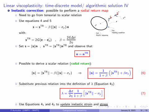
Linear viscoplasticity: time-discrete model/ algorithmic solution IVInelastic correction: possible to perform a radial return map

Need to go from tensorial to scalar relation

Use equations 4 and 5

s = sTR − β (‖s‖ − σy ) n

with:

sTR = 2G(e− ein) , β =2G∆t

2η Set s = ‖s‖n , sTR = ‖sTR‖nTR and observe that

n = nTR

Possible to derive a scalar relation (radial return):

‖s‖ = ‖sTR‖ − β (‖s‖ − σy ) ⇒ ‖s‖ =1

1 + β

(

‖sTR‖+ βσy

)

(6)

Substitute previous relation into the definition of λ (Equation 43)

λ =∆t

2η

1

1 + β

[

‖sTR‖ − σy

]

(7)

Use Equations 41 and 42 to update inelastic strain and stress


Linear viscoplasticity: time-discrete model/ algorithmic solution V

Algorithmic-consistent tangent tensor Ctgdisc


Linearize deviatoric elastic and inelastic strain evolution equations

s = 2G(e− ei )

ei = ein + λnTR

⇒

ds = 2G(de− dei )

dei = nTRdλ+ λdnTR

Linearize λ

λ =∆t

2η

1

1 + β

[

‖sTR‖ − σy

]

⇒ dλ = AdiscnTR : de

with:

Adisc =2G∆t

2η + 2G∆t

Recall

nTR =sTR

‖sTR‖ =sTR

[

(sTR : sTR)12

]


Linear viscoplasticity: time-discrete model/ algorithmic solution VI

Linearize nTR

dnTR =1

‖sTR‖[

I− (nTR ⊗ nTR)]

dsTR =N

TR

‖sTR‖dsTR

where:

NTR =

1

‖sTR‖[

I− (nTR ⊗ nTR)]

with NTR orthogonal projection on plane with unit normal nTR = n

NTRnTR = 0 and N

TRN

TR = NTR

Since dsTR = 2Gde, obtain

dnTR = 2GN

TR

‖sTR‖de


Linear viscoplasticity: time-discrete model/ algorithmic solution VII

Combining all previous relations

ds =[

2G(1− C)II + 2G (C − Adisc)(nTR ⊗ nTR)

]

de

with:

C =2Gλ

‖sTR‖

Recalling volumetric-deviatoric stress split, get algorithmic tangent tensor

Ctgdisc = K (I⊗ I) + 2G (1− C) Idev + 2G (C − Adisc)(n

TR ⊗ nTR)


Linear viscoplasticity: time-discrete model/ algorithmic solution VIII

Given σn,εεεn, ein and εεε

Compute en, θn and eCompute trial state [ Eq. 5 ]Check trial stateIf ( ‖sTR‖ > σy ) then

Plastic stepCompute λ [ Eq. 7 ]Update ei [ Eq. 4 ]Update s and p [ Eq. 4 ]Compute algorithmic tangent [ Eq. 28 ]

ElseElastic step

Update s and p with trial state [ Eq. 5 ]Compute elastic tangent

End ifCompute stress σ

Exit


Classical plasticity I

Classical plasticity

Classical plasticity theory is based on blanket assumption of “rate-independent” plasticity, i.e. inelastic deformation takes place only when:

F = 0 , F = 0

the latter known as consistency condition or persistence condition


Classical plasticity II

Conventional to indicate inelastic strain as εεεp

Additive strain decomposition written as

εεε = εεεe + εεε

p

Evolution function g written through a factor γ to emphasize that it is a rate factor(though not time derivative of a state variable γ)

Internal variable ξ evolves as

ξ = γh where

γ =1

H

⟨

F

⟩

if F = 0

γ = 0 if F < 0

with

F=∂F

∂σ: σ , H = −∂F

∂ξ: h

∂F/∂σ = ∇σF : gradient of yield function

F : projection of σ on yield surface normal H > 0: material hardening


J2 classical plasticity: time-continuous model I

A simple J2 plasticity model

Model assumptions:

Isotropic linear elastic response

Accordingly

θe =p

K, ee =

s

2G

Von Mises or J2 materials

Yield function F depends only on deviatoric stress norm ‖s‖ =√2J2

Accordingly

θp = 0 , εεεp = ep

No hardening mechanisms


J2 classical plasticity: time-continuous model II

Model equations

Standard part →

p = K θ

s = 2G (e− ep)

F = ‖s‖ − σy

Novelty part →

ep = γ n

γ ≥ 0 , F ≤ 0 , γF = 0

where in the order we have

volumetric elastic relation with p pressure, θ volumetric strain, K bulk modulus

deviatoric elastic relation with G shear modulus

von Mises yield function

⋆ deviatoric plastic strain evolution (associative plasticity)

n =∂F

∂s=

s

‖s‖

⋆ Kuhn-Tucker conditions (converting plastic problem to constrained optimization one)


J2 classical plasticity: time-discrete couterpart and integration algorithm I

Goal: develop time-discrete counterpart for numerical solution

Backward Euler to integrate evolutionary equation

Return map algorithm to solve non-linearity

Address elasto-plastic tangent tensor consistent with discrete algorithmic model

Let [0,T ] ⊂ R be a time interval

Focus on two time values, tn and tn+1, with tn+1 time value of interest after tn

To minimize subscript appearance (to make equations more readable)

an = a(tn) , a = a(tn+1)

→ Quantity evaluated at tn: subscript n

→ Quantity evaluated at tn+1: no subscript



J2 classical plasticity: time-discrete couterpart and integration algorithm II

IDEA: compute stress history from strain history (strain driven problem)Given strain εεε at tn+1 and solution at tn (i.e. σn, εεεn, e

in), compute solution at tn+1

Backward Euler integration formula for plastic strain evolution

ep = epn + λ n with λ =

∫ tn+1

tn

γ dt

Substitute into elastic constitutive relation

s = 2G [e− epn]− 2G λ n


ep = γ n

s = 2G [e− ep ]

F = ‖s‖ − σy

γ ≥ 0 , F ≤ 0 , γF = 0

⇒

ep = epn + λn

s = 2G [e− epn ] + 2Gλn

F = ‖s‖ − σy

λ ≥ 0 , F ≤ 0 , λF = 0

⋆ λ and n are unknown quantities to be computed by return map algorithm


J2 classical plasticity: time-discrete couterpart and integration algorithm III

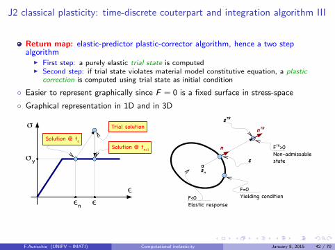
Return map: elastic-predictor plastic-corrector algorithm, hence a two stepalgorithm

First step: a purely elastic trial state is computed Second step: if trial state violates material model constitutive equation, a plastic

correction is computed using trial state as initial condition

Easier to represent graphically since F = 0 is a fixed surface in stress-space

Graphical representation in 1D and in 3D


J2 classical plasticity: time-discrete couterpart and integration algorithm IVTrial state: assume no plastic deformation in [tn, tn+1]

Assume ep = epn, λ = 0 Compute elastic trial state

λTR = 0

ep,TR = epn

sTR = 2G [e− epn ]

(8)

Check trial state: if elastic trial state (i.e. ‖sTR‖ ≤ σy ) is admissible, then trial state does not violate model trial state represents solution at tn+1 following part of algorithm can be skipped

Plastic correction: if trial state (‖sTR‖ > σy) is non-admissible, then trial state does violate model hence a correction should be performed enforce limit equation to compute discrete plastic rate λ


Discrete plastic parameter and plastic rate parameter I

Plastic correction: enforce limit equation F = 0 to compute discrete plastic rate λ Express elastic relation and plastic evolution in terms of trial state and λ

ep = epn + λn

s = 2G [e− epn ] + 2Gλn⇒

ep = ep,TR + λn

s = sTR − 2G λ n

Last relation implies n = nTR hence a scalar relation may be derived

‖s‖ = ‖sTR‖ − 2Gλ

Discrete form of limit equation can be enforced

F = ‖s‖ − σy = 0 ⇒ F =[

‖sTR‖ − 2Gλ]

− σy = 0

Discrete form of limit equation can be solved for λ

λLP =‖sTR‖ − σy

2G

Discrete plastic rate parameter λ computed solving a scalar equation


Discrete plastic parameter and plastic rate parameter II

Closest point projection of trial state onto limit surface F = 0 reduces to radialprojection

n = nTR


Discrete elasto-plastic tangent tensor I

Algorithmic-consistent tangent tensor Ddisc

⋆ Use of a consistent tangent tensor preserves quadratic convergence of a Newtonmethod, for example within incremental solution in a finite element scheme

⋆ Almost identical to visco-plasticity

Linearize deviatoric elastic and inelastic strain evolution

s = 2G(e− ep)

ep = epn + λnTR

⇒

ds = 2G(de− dep)

dep = nTRdλ+ λdnTR

Linearize sTR, ‖sTR‖, λ

sTR = 2G (e− epn)

‖sTR‖ =√sTR : sTR

λ =‖sTR‖ − σy

2G

⇒

dsTR = 2Gde

d‖sTR‖ =sTR

‖sTR‖ : dsTR

dλ =d‖sTR‖2G

dsTR = 2Gde

d‖sTR‖ = 2GnTR : de

dλ = nTR : de


Discrete elasto-plastic tangent tensor II

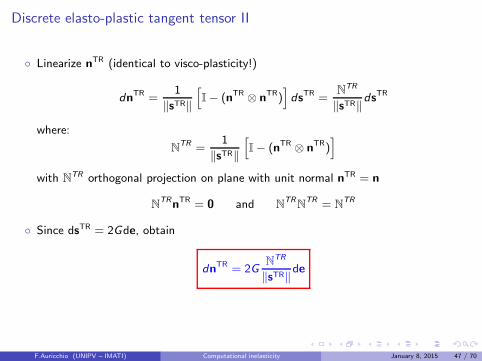
Linearize nTR (identical to visco-plasticity!)

dnTR =1

‖sTR‖[

I− (nTR ⊗ nTR)]

dsTR =N

TR

‖sTR‖dsTR

where:

NTR =

1

‖sTR‖[

I− (nTR ⊗ nTR)]


NTRnTR = 0 and N

TRN

TR = NTR

Since dsTR = 2Gde, obtain

dnTR = 2GN

TR

‖sTR‖de


Discrete elasto-plastic tangent tensor III

Accordingly, deviatoric elastic relation can be recast as follows

ds = 2G[

I− C NTR]

de− 2GnTRdλ

where:

C =2Gλ

‖sTR‖ Assume linearization of discrete limit equation in the form

dλ = Adisc[nTR : de]

with Adisc a scalar quantity (for LP Adisc = 1)

Accordingly, deviatoric elastic relation simplifies to

ds = 2G[

I− C NTR − Adisc

(

nTR ⊗ nTR)]

de


Discrete elasto-plastic tangent tensor IV

Combine with incremental elastic volumetric relation and obtain

dσ = Ddiscdεεε

Algorithmic elasto-plastic tangent tensor given by

Ddisc = K (I⊗ I) + 2G (1− C) Idev + 2G (C − Adisc)(n⊗ n)

⋆ Ddisc consistent with discrete model

⋆ Ddisc symmetric

⋆ Ddisc = Dcont when C LP = 0 or when load step reduces to zero


A slightly more general plasticity model I

Complexity of material response under cyclic conditions


A slightly more general plasticity model II

Lemaitre-Chaboche, Mechanics of Solid Materials, Cambridge University Press, 1990

Besson, Cailletaud, Chaboche, Forest, Non-Linear Mechanics of Materials Springer, 2010


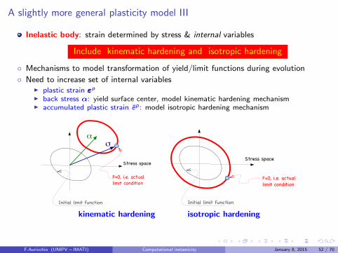
A slightly more general plasticity model III

Inelastic body: strain determined by stress & internal variables

Include kinematic hardening and isotropic hardening

Mechanisms to model transformation of yield/limit functions during evolution

Need to increase set of internal variables plastic strain εεεp

back stress α: yield surface center, model kinematic hardening mechanism accumulated plastic strain ep: model isotropic hardening mechanism

kinematic hardening isotropic hardening


J2 plasticity with linear hardening: time-continuous model I

A J2 plasticity model with simple (linear!) hardening

Model assumptions:

Isotropic linear elastic response

Accordingly

θe =p

K, ee =

s

2G

Von Mises or J2 materials

Yield function F depends only on deviatoric stress norm ‖s‖ =√2J2

Accordingly

θp = 0 , εεεp = ep

Simple hardening mechanisms

Linear kinematic Linear isotropic


J2 plasticity with linear hardening: time-continuous model II

Model equations

p = K θ

s = 2G (e− ep)

ep = γ n

Σ = s−α

α = Hkinep = Hkinγn

F = ‖Σ‖ − σy (ep)

σy(ep) = σy,0 + Hiso e

p

˙ep = ‖ep‖ = γ

γ ≥ 0 , F ≤ 0 , γF = 0

⋆ Still associative plasticity, in fact deviatoric plastic strain evolution

n =∂F

∂σ=

∂F

∂Σ=

Σ

‖Σ‖

Two new internal variable: back stress α and accumulative plastic strain ep

von Mises yield function now expressed in terms of the relative stress Σ


Linear hardening J2 plasticity: time-discrete and integration algorithm I

Goal: develop time-discrete counterpart for numerical solution

Backward Euler to integrate evolutionary equation

Return map algorithm to solve non-linearity

Address elasto-plastic tangent tensor consistent with discrete algorithmic model

Let [0,T ] ⊂ R be a time interval

Focus on two time values, tn and tn+1, with tn+1 time value of interest after tn

To minimize subscript appearance (to make equations more readable)

an = a(tn) , a = a(tn+1)

→ Quantity evaluated at tn: subscript n

→ Quantity evaluated at tn+1: no subscript



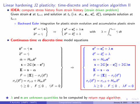
Linear hardening J2 plasticity: time-discrete and integration algorithm IIIDEA: compute stress history from strain history (strain driven problem)Given strain εεε at tn+1 and solution at tn (i.e. σn, εεεn, e

pn , e

pn ), compute solution at

tn+1

Backward Euler integration for plastic strain evolution and accumulative plastic strain

ep = γ n

˙ep = γ

⇒

ep = epn + λ n

ep = epn + λwith λ =

∫ tn+1

tn

γ dt


ep = γ n

˙ep = γ

α = Hkinep

s = 2G (e− ep)

Σ = s−α

F = ‖Σ‖ − σy (ep)

σy (ep) = σy,0 + Hiso e

p

γ ≥ 0 , F ≤ 0 , γF = 0

⇒

ep = epn + λ n

ep = e

pn + λ

α = Hkinep

s = 2G [e− epn ] + 2Gλn

Σ = s−α

F = ‖Σ‖ − σy(ep)


p

λ ≥ 0 , F ≤ 0 , λF = 0

⋆ λ and n are unknown quantities to be computed by return map algorithm


Linear hardening J2 plasticity: time-discrete and integration algorithm III

Return map: elastic-predictor plastic-corrector algorithm, hence a two stepalgorithm

First step: a purely elastic trial state is computed Second step: if trial state violates material model constitutive equation, a plastic

correction is computed using trial state as initial condition

Easier to represent graphically since F = 0 is a fixed surface in stress-space

Graphical representation in 1D and in 3D


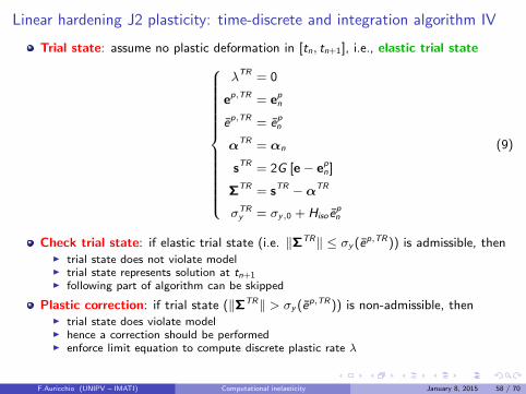
Linear hardening J2 plasticity: time-discrete and integration algorithm IV

Trial state: assume no plastic deformation in [tn, tn+1], i.e., elastic trial state

λTR = 0

ep,TR = epn

ep,TR = e

pn

αTR = αn

sTR = 2G [e− epn]

ΣTR = sTR −αTR

σTRy = σy,0 + Hiso e

pn

(9)

Check trial state: if elastic trial state (i.e. ‖ΣTR‖ ≤ σy (ep,TR)) is admissible, then

trial state does not violate model trial state represents solution at tn+1 following part of algorithm can be skipped

Plastic correction: if trial state (‖ΣTR‖ > σy (ep,TR)) is non-admissible, then

trial state does violate model hence a correction should be performed enforce limit equation to compute discrete plastic rate λ


Discrete plastic parameter and plastic rate parameter I

Plastic correction: enforce limit equation F = 0 to compute discrete plastic rate λ Express elastic relation and plastic evolution in terms of trial state and λ

ep = epn + λn

s = 2G [e− epn] + 2Gλn

Σ = s−α


p

⇒

ep = ep,TR + λn

s = sTR − 2G λ n

Σ = ΣTR − (2G + Hkin) λn

σy (ep) = σTR

y + Hisoλ

Last relation implies n = nTR hence a scalar relation may be derived

‖Σ‖ = ‖ΣTR‖ − (2G + Hkin)λ

Discrete form of limit equation can be enforced

F = ‖Σ‖ − σy = 0 ⇒ F =[

‖ΣTR‖ − (2G + Hkin)λ]

−(

σTRy + Hisoλ

)

= 0

Discrete form of limit equation can be solved for λ

λLP =‖ΣTR‖ − σTR

y

2G + Hiso + Hkin

Discrete plastic rate parameter λ computed solving a scalar equation


Discrete elasto-plastic tangent tensor I

Algorithmic-consistent tangent tensor Ddisc

⋆ Use of a consistent tangent tensor preserves quadratic convergence of a Newtonmethod, for example within incremental solution in a finite element scheme

⋆ Almost identical to visco-plasticity

Linearize deviatoric elastic and inelastic strain evolution

s = 2G(e− ep)

ep = epn + λnTR

⇒

ds = 2G(de− dep)

dep = nTRdλ+ λdnTR

We need to linearize nTR and λ

To linearize nTR, we need to linearize ΣTR , ‖ΣTR‖, λ


Discrete elasto-plastic tangent tensor II

Linearize ΣTR , ‖ΣTR‖, λ

sTR = 2G (e− epn)

‖ΣTR‖ =√

ΣTR : ΣTR

λ =‖ΣTR‖ − σy

2G + Hiso + Hkin

dsTR = 2Gde

d‖ΣTR‖ =ΣTR

‖ΣTR‖: dΣTR

dλ =1

2G + Hiso + Hkin

(

d‖ΣTR‖ − dσTRy

)

dsTR = 2Gde

d‖ΣTR‖ = 2GnTR : de

dλ = AdiscnTR : de

with Adisc =2G

2G + Hiso + Hkin


Discrete elasto-plastic tangent tensor III

Linearize nTR (identical to visco-plasticity!)

dnTR =1

‖ΣTR‖

[

I− (nTR ⊗ nTR)]

dΣTR =N

TR

‖ΣTR‖dΣTR

where:

NTR =

1

‖ΣTR‖

[

I− (nTR ⊗ nTR)]


NTRnTR = 0 and N

TRN

TR = NTR

Since dΣTR = dsTR = 2Gde, obtain

dnTR = 2GN

TR

‖ΣTR‖de


Discrete elasto-plastic tangent tensor IV

Accordingly, deviatoric elastic relation can be recast as follows

ds = 2G[

I− C NTR]

de− 2GnTRdλ

where:

C =2Gλ

‖ΣTR‖ Assume linearization of discrete limit equation in the form

dλ = Adisc[nTR : de]

with Adisc a scalar quantity

Accordingly, deviatoric elastic relation simplifies to

ds = 2G[

I− C NTR − Adisc

(

nTR ⊗ nTR)]

de


Discrete elasto-plastic tangent tensor V

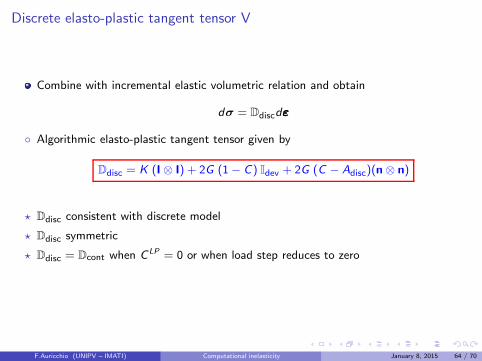
Combine with incremental elastic volumetric relation and obtain

dσ = Ddiscdεεε

Algorithmic elasto-plastic tangent tensor given by

Ddisc = K (I⊗ I) + 2G (1− C) Idev + 2G (C − Adisc)(n⊗ n)

⋆ Ddisc consistent with discrete model

⋆ Ddisc symmetric

⋆ Ddisc = Dcont when C LP = 0 or when load step reduces to zero


A more general plasticity model: time-continuous scheme I

A more general plasticity model

Model equations:


p

εεεe = εεε

e(σ)

F = f (σ)− σy

εεεp = γ

∂F

∂σ

γ ≥ 0 , F ≤ 0 , γF = 0

Model assumptions:

Additive strain decomposition

General elastic response

General yield function F

Associative flow rule

No hardening mechanisms


A more general plasticity model: time-continuous scheme II

Integration in time: standard backward Euler


p

εεεe = εεε

e(σ)

F = f (σ)− σy

εεεp = γ

∂F

∂σ

γ ≥ 0 , F ≤ 0 , γF = 0

⇒


p

εεεe = εεε

e(σ)

F = f (σ)− σy

εεεp = εεε

pn + λ

∂F

∂σ

λ ≥ 0 , F ≤ 0 , λF = 0

Solution algorithm: standard predictor-corrector (return map!)

Interesting to explore the plastic correction


A more general plasticity model: time-continuous scheme III

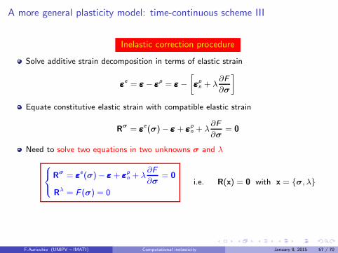
Inelastic correction procedure

Solve additive strain decomposition in terms of elastic strain

εεεe = εεε− εεε

p = εεε−[

εεεpn + λ

∂F

∂σ

]

Equate constitutive elastic strain with compatible elastic strain

Rσ = εεεe(σ)− εεε+ εεε

pn + λ

∂F

∂σ= 0

Need to solve two equations in two unknowns σ and λ

Rσ = εεεe(σ)− εεε+ εεε

pn + λ

∂F

∂σ= 0

Rλ = F (σ) = 0

i.e. R(x) = 0 with x = σ, λ


A more general plasticity model: time-continuous scheme IV

In general, non-linear system solved using some iterative method, e.g., Newton

R(xi+1) = 0 ⇒ R(xi ) +∂R

∂x

∣

∣

∣

∣

∣

i

∆x = 0

∂R

∂x= Ktg =

∂Rσ

∂σ

∂Rσ

∂λ

∂Rλ

∂σ

∂Rλ

∂λ

=

Del,tg + λ

∂2F

∂σ2

∂F

∂σ(

∂F

∂σ

)T

0

with Del,tg =

∂εεεe

∂σ


A more general plasticity model: time-continuous scheme V

Time-discrete consistent tangent

Linearize residual

R(x,εεε) = R(σ, λ,εεε) = 0 ⇒ dR =∂R

∂xdx+

∂R

∂εεεdεεε = 0

Solve wrt dx

dx = −[

∂R

∂x

]

−1∂R

∂εεεdεεε

Note that

Ktg =∂R

∂xand

∂R

∂εεε=

I

0

x =

σ

λ

Accordingly

∂σ

∂εεε=

([

∂R

∂x

]

−1)

11


Bibliography I

O.C. Zienkiewicz, R.L. Taylor, D.D. Fox, The Finite Element Method for Solid and Structural Mechanics.

Butterworth-Heinemann (2014)

J.C. Simo and T.J.R. Hughes, Computational inelasticity. Springer-Verlag (1998)

J.C. Simo, Topics on the numerical analysis and simulation of plasticity. In P. Ciarlet and J. Lions (Eds.),Handbook of numerical analysis, Volume III. Elsevier Science Publisher B.V. (1999)

E.A. de Souza Neto, D Peric, DRJ Owen, Computational methods for plasticity: theory and applications.Wiley (2008)


NONLINEAR COMPUTATIONAL SOLID & …...NONLINEAR COMPUTATIONAL SOLID & STRUCTURAL MECHANICS...

Documents

Transcript of NONLINEAR COMPUTATIONAL SOLID & …...NONLINEAR COMPUTATIONAL SOLID & STRUCTURAL MECHANICS...