Nonlinear collective phase dynamics of limit-cycle ...

Nonlinear collective phase dynamics

of limit-cycle oscillator lattices

Roland Lauter

Nonlinear collective phase dynamics

of limit-cycle oscillator lattices

Nichtlineare kollektive Phasendynamik

von Grenzzyklus-Oszillatoren auf Gittern

Der Naturwissenschaftlichen Fakultät

der Friedrich-Alexander-Universität Erlangen-Nürnberg

zur

Erlangung des Doktorgrades Dr. rer. nat.

vorgelegt von

Roland Lauter

aus Eichstätt

Als Dissertation genehmigtvon der Naturwissenschaftlichen Fakultätder Friedrich-Alexander-Universität Erlangen-Nürnberg

Tag der mündlichen Prüfung: 16.12.2016

Vorsitzender des Promotionsorgans: Prof. Dr. Georg KreimerGutachter: Prof. Dr. Florian MarquardtGutachter: Prof. Dr. Michael Schmiedeberg

Contents

1 Introduction: Effective phase models and coupled optomechanical systems 11.1 Effective phase models for nonlinear oscillators . . . . . . . . . . . . . . . . . . 11.2 Optomechanics of a single optical mode coupled to a single mechanical mode 4

1.2.1 The optomechanical interaction . . . . . . . . . . . . . . . . . . . . . . . 41.2.2 The classical equations of motion . . . . . . . . . . . . . . . . . . . . . . 71.2.3 Classical nonlinear dynamics . . . . . . . . . . . . . . . . . . . . . . . . 8

1.3 Optomechanical arrays . . . . . . . . . . . . . . . . . . . . . . . . . . . . . . . . . 101.4 Outline of this thesis . . . . . . . . . . . . . . . . . . . . . . . . . . . . . . . . . . 12

2 The Hopf-Kuramoto model for the mechanical phases in optomechanical arrays 152.1 The Hopf equations for a single optomechanical cell . . . . . . . . . . . . . . . 152.2 Derivation of the effective mechanical phase equations of an optomechanical

array . . . . . . . . . . . . . . . . . . . . . . . . . . . . . . . . . . . . . . . . . . . . 172.3 Previous results for the Hopf-Kuramoto model . . . . . . . . . . . . . . . . . . . 19

3 Relation to models of nonlinear dynamics and statistical physics 233.1 The Kuramoto model and synchronization . . . . . . . . . . . . . . . . . . . . . 233.2 The Kuramoto-Sakaguchi model and pattern formation . . . . . . . . . . . . . 263.3 The XY model and the Kosterlitz-Thouless transition . . . . . . . . . . . . . . . 30

4 Deterministic dynamics and pattern formation in the Hopf-Kuramoto model 354.1 Pattern phase diagram for two-dimensional arrays of coupled limit-cycle os-

cillators . . . . . . . . . . . . . . . . . . . . . . . . . . . . . . . . . . . . . . . . . . 364.1.1 Pattern formation . . . . . . . . . . . . . . . . . . . . . . . . . . . . . . . 374.1.2 Experimental implementation . . . . . . . . . . . . . . . . . . . . . . . . 424.1.3 Semi-analytical stability analysis of point defects . . . . . . . . . . . . . 434.1.4 Read-out of the mechanical resonator phase field . . . . . . . . . . . . 44

4.2 Pattern formation in one-dimensional arrays . . . . . . . . . . . . . . . . . . . . 464.2.1 Straight lines and jump defects in the case of overdamped dynamics . 464.2.2 Propagating zigzag structures in the Kuramoto-Sakaguchi model . . . 48

v

5 Stochastic dynamics and phase-field roughening in the Hopf-Kuramoto model 535.1 Slope selection in the overdamped dynamics of one-dimensional arrays . . . . 545.2 The influence of noise on the properties of spirals . . . . . . . . . . . . . . . . . 565.3 The Kardar-Parisi-Zhang model of surface growth . . . . . . . . . . . . . . . . . 625.4 From Kardar-Parisi-Zhang scaling to explosive desynchronization in arrays of

limit-cycle oscillators . . . . . . . . . . . . . . . . . . . . . . . . . . . . . . . . . . 655.4.1 Context and model . . . . . . . . . . . . . . . . . . . . . . . . . . . . . . . 655.4.2 Relation to the Kardar-Parisi-Zhang model . . . . . . . . . . . . . . . . . 685.4.3 Dynamics in one-dimensional systems . . . . . . . . . . . . . . . . . . . 695.4.4 Dynamics in two-dimensional systems . . . . . . . . . . . . . . . . . . . 745.4.5 Methods . . . . . . . . . . . . . . . . . . . . . . . . . . . . . . . . . . . . . 76

6 Conclusion and outlook 79

A Methods 83A.1 Study of the deterministic Hopf-Kuramoto model . . . . . . . . . . . . . . . . . 83A.2 Study of the stochastic Hopf-Kuramoto model . . . . . . . . . . . . . . . . . . . 87

Bibliography 93

List of publications 105

Abstract in German 107

Abstract

Coupled limit-cycle oscillators exhibit interesting collective phenomena, like synchroniza-tion and pattern formation. Effective models of the classical phase dynamics in these systemshave been very successful in describing these effects. Important examples are the canonicalKuramoto model and the Kuramoto-Sakaguchi model. In this thesis, we study a closely re-lated, slightly more general effective phase model, which we call Hopf-Kuramoto model. Wefocus on the phase dynamics in one-dimensional and two-dimensional lattices.

One central topic is the pattern formation in the deterministic model. As a main result,we present the pattern phase diagram for two-dimensional arrays. This diagram illustrateswhich patterns are relevant in the long-time dynamics, after starting from random initialconditions, in dependence on the parameters of the model. We examine details of impor-tant stationary and non-stationary patterns. This includes the shape and movement of spiralstructures, as well as their influence on correlations. Regarding one-dimensional systems, wefind smooth stationary patterns with characteristic defects and solitary-wave-like structuresin different limiting cases of our model.

Subsequently, we discuss the stochastic dynamics. We study the effects of noise on someof the patterns found in the deterministic case. We then continue with an analysis of a lim-iting case of the Hopf-Kuramoto model, the noisy Kuramoto-Sakaguchi model. For smoothphase fields, this model is related to the Kardar-Parisi-Zhang model of surface growth. Thisenables us to explain scaling properties of the phase field with time, as well as a suddendesynchronization process which we find in simulations.

As an example of a system where our model is applicable, we discuss future optomechan-ical arrays. Moreover, we show that the derivation of the Hopf-Kuramoto model is based onvery general assumptions about the dynamics of nonlinear oscillators close to their limit cy-cle. Hence, our results are relevant for a large class of experiments on arrays of locally coupledoscillators.

ix

Chapter 1

Introduction: Effective phase modelsand coupled optomechanical systems

1.1 Effective phase models for nonlinear oscillators

In this thesis, we investigate the classical phase dynamics of coupled nonlinear oscillators,which are driven individually into self-sustained oscillations. The essential building block ofsuch a system is a nonlinear oscillator to which energy is supplied by some driving mecha-nism. In a typical physical system, the oscillator will have some internal damping, for exam-ple because of friction. Hence, if the driving is weak, the oscillator will eventually come to arest. However, if the driving is strong enough, the internal damping can be overcome and theoscillator might move forever. This can lead to complicated, maybe even chaotic, behavior.

But there is also an important, simpler case, which we will focus on. That is, the oscilla-tor might eventually perform periodic motion. This means that it returns to the same statesover and over again, after some fixed time interval. Thus, if we start at one of these states,the trajectory in the phase space of the system will be closed. Moreover, we will only con-sider systems where close-by trajectories will converge to the periodic one. Then, this spe-cial, loop-like solution of the time evolution of our system is called a stable limit cycle. For amore rigorous definition of this term, see [1]. In the situation described above, we speak of aself-sustained oscillator or a limit-cycle oscillator.

Note that the famous harmonic oscillator does not constitute such a system: If its am-plitude is changed slightly, for example by a sudden kick, it will continue its motion on adifferent closed trajectory, see Fig. 1.1a. This changes if we consider the driven and dampedharmonic oscillator, see Fig. 1.1b: After a perturbation from the periodic trajectory, it will re-turn to this characteristic motion for long times. However, from a conceptual point of view,this is not a limit-cycle oscillator because the closed trajectory is not described by an au-tonomous system of differential equations (as the drive explicitly depends on time). One ofthe consequences of this is that the phase of the oscillator actually depends on the phase of

1

Chapter 1. Introduction: Effective phase models and coupled optomechanical systems

−0.2 0.0 0.2

−0.2

0.0

0.2

−0.2 0.0 0.2

−0.2

0.0

0.2

−2 0 2

−2

0

2a b c

mom

entu

m

position

limit cycle

Figure 1.1: Phase space portraits of different oscillators. (a) The classical harmonic oscillator.It performs periodic motion, see, for example, the red line. When the oscillator is perturbed(as indicated by the red arrows), it continues its motion in a different region of phase space(black and blue lines), even for very long times. Because the closed trajectories can be ar-bitrarily close to each other, we do not have a limit cycle here. (b) The driven and dampedharmonic oscillator. In the long-time limit, the oscillator will perform periodic motion, seethe red line. If the system is perturbed, it will return to that specific trajectory. Because ofthe fixed relation to the drive, we will actually find the system in the same state after a longtime (see blue and black dots) for any perturbation. The reason is that the system is not au-tonomous, which is why we do not speak of a limit cycle here. (c) The van der Pol oscillator.This is a typical nonlinear oscillator exhibiting a limit cycle (red line in the plot). After a per-turbation, the trajectories converge to this cycle, which indicates its stability. Because there isno preferred phase, we will in general find different states on the limit cycle after a long time(blue and black dots), associated with different phases. This illustrates the special role of thephase degree of freedom for limit-cycle oscillators.

the drive. Hence, for different perturbations, we will find the system in the same state after agiven long time. This is indicated by the overlapping blue and black dots in Fig. 1.1b.

In contrast, the phase of the periodic motion of a nonlinear oscillator might not dependon the (potentially existing) phase of the drive. Hence, this system actually offers a largerflexibility. Moreover, this property makes self-sustained oscillators very sensitive to influ-ences from the environment, because changes of the phase will not be reset by the drivingmechanism. For example, if we artificially change the phase of an isolated limit-cycle oscil-lator by an amount δϕ at some point in time, this change will persist forever and can alsobe detected a long time later. On the contrary, if the amplitude of the nonlinear oscillator ischanged slightly, that is if we move the system away from the limit cycle, the behavior is quitedifferent: The system will relax back to the periodic motion of the limit cycle, it will basically“forget” about the amplitude change. It is only because the phase dynamics might dependon the value of the amplitude that this process can still leave behind changes in the phase.

2

1.1. Effective phase models for nonlinear oscillators

Thus, we will in general find different states, characterized by different phases, after variousperturbations. This is illustrated by the blue and black dots in Fig. 1.1c, where we displayphase space portraits of a canonical nonlinear system, the Van der Pol oscillator.

So far, we did not specify exactly what the phase of an oscillator is. For the harmonic os-cillator and other two-coordinate systems with a circular trajectory in phase space, we cansimply identify the phase with the angular coordinate of the point in phase space which de-scribes the state of the system. For nonlinear oscillators, which can have very complicatedlimit cycles in phase space, it is more useful to define the phase in a more general way: On thelimit cycle, the phase is defined to grow linearly with time, such that it increases by 2π withinone period of the oscillation. This notion can be extended to the vicinity of the limit cycle,see [1] for the procedure. For circular limit cycles, this actually leads to the simple definitionof the phase mentioned before.

The discussion above illustrates that the phase is, in some sense, the most important andthe outstanding degree of freedom of a self-sustained oscillator. For this reason, one oftentries to reduce the description of such a physical system (in terms of equations of motion forits many degrees of freedom) to an effective description in terms of a differential equationfor the phase only. Of course, this effective equation still has to include indirect influenceson the phase, as they appear when some environment acts on the amplitude (which mightalso affect the phase dynamics, as mentioned above). Hence, the effective equation mightstill be highly nonlinear and hard to tackle. But in many cases, this is still better than tryingto understand the complicated dynamics of the full system.

This is particularly relevant if one does not study a single self-sustained oscillator, but in-stead tries to analyze the behavior of many such elements, which are coupled to each other.In this situation, the oscillators influence each other. For example, the phase of one oscilla-tor might affect the amplitude dynamics of another oscillator. In the complete description,this leads to a large set of coupled differential equations. Even in the simplest case wherewe only have to consider differential equations of first order in time, and where each oneof N oscillators is described only by its amplitude and phase, we still get 2N coupled equa-tions. Moreover, as we argued above, the amplitude dynamics might not be interesting at all.Hence, it makes sense to try to derive effective equations for the phases of coupled limit-cycleoscillators. This allows one to focus on the most prominent effects of the coupling.

One of these effects is that limit-cycle oscillators, which run at different natural frequen-cies when they are on their own, can actually agree on a common effective frequency whenthey are weakly coupled. This effect is called synchronization and has been found in manynatural and engineered systems [1]. In our context, it is important to note that roughly 40years ago, it was found out by Y. Kuramoto that this phenomenon can actually be under-stood by an effective phase model [2, 3]. Furthermore, coupled oscillators can not only adjusttheir rhythms, but also the relative phase values themselves. This is particularly interestingin locally coupled systems (called oscillator lattices, see also Fig. 5.5a), where regular phasepatterns can emerge. This phenomenon of pattern formation has been found in biological,chemical and physical systems, see [4]. In some cases, effective phase models can explain

3


this surprising self-organization.In this thesis, we will apply the ideas presented above to the physical system of coupled

optomechanical cells, which will be introduced in the following sections. First, we will showhow a single optomechanical cell can be driven into self-sustained oscillations. Arrangedon a regular lattice, these cells can form optomechanical arrays. If the cells are coupled toeach other, we have the situation described above, a set of coupled self-sustained oscillators.This enables us to derive an effective phase model, which we will call the Hopf-Kuramotomodel. As we will see, this model is actually applicable to a wide variety of coupled limit-cycle oscillators. It is the analysis of this model which is the main subject of this thesis. Inparticular, we will discuss effects in large lattices, in the context of two of the phenomenamentioned above, synchronization and pattern formation.

1.2 Optomechanics of a single optical mode coupled to a singlemechanical mode

In this section, we will present the canonical cavity optomechanical setup, which can be de-scribed as an interacting system of one optical and one mechanical mode. We will focus onthe classical aspects, in particular on the nonlinear dynamics of this system. As outlined inthe previous section, this is particularly relevant for us because we will find the possibility ofself-sustained oscillations.

1.2.1 The optomechanical interaction

When light is reflected from an object, it transfers momentum to that object. This can be un-derstood easily if we think of the individual photons bouncing off the surface: Each photoncarries momentum, directed in the propagation direction. After the reflection, this directionis different than before, and the difference in momentum has been transferred to the reflect-ing object because of momentum conservation. A change in momentum is equivalent to aforce. Hence, in other words, light exerts radiation pressure force on mechanical objects uponreflection. This effect is called the optomechanical interaction.

Under usual circumstances on earth, this effect is very tiny so that it does not play a role.For example, the mechanical object might be so heavy that its change in momentum is notrecognizable. Moreover, when light hits an object, there are other effects such as heating (be-cause of absorption), which might obscure the influence of the optomechanical interaction.This made it difficult to provide evidence for the existence of the radiation pressure force inearly experiments [5, 6]. In outer space, however, this force can actually have an importantimpact. For example, this leads to the fact that dust tails of comets point away from the sun,as was already recognized by Kepler [7]. Nowadays, there are first attempts to use the radia-tion pressure force for the impulsion of spacecraft with so-called “light sails”.

In laboratory systems, the optomechanical interaction can be engineered to become im-portant by using mechanical objects with small masses and very intense light sources. Typi-

4

1.2. Optomechanics of a single optical mode coupled to a single mechanical mode

laser drive

optical cavitymovable mirror

frequency !L resonance frequency!cav(x)

displacement x

Figure 1.2: The standard optomechanical setup. It consists of an optical cavity where oneend-mirror is movable. Its displacement x influences the resonance frequency of the cavityωcav(x). Usually, the cavity is driven by a laser with some frequency ωL. Because of the ra-diation pressure force, the resulting light field inside the cavity influences the position of themechanics. This is the origin of the cavity-optomechanical interaction.

cally, the mechanical element is a highly reflective mirror, mounted on some support, whichmeans that it can be treated as a harmonic oscillator. A monochromatic laser is usually takenas the light source, and it is enhanced by using a cavity, where one of the end-mirrors is themechanical element. For an illustration of this setup, see Fig. 1.2. Setups like this are con-sidered in the research field of cavity optomechanics. An important feature here is that themotion of the mechanical element now acts back on the light field because the resonancefrequency of the cavity depends on the position of the mechanics. This characteristic depen-dency appears not only in the simple cavity system described above, but also in many othermodern experiments with localized optical and mechanical modes, as we will see later. Thismakes the formalism of cavity optomechanics widely applicable. For comprehensive reviewsabout this field, see [8, 9].

We now want to go into more detail and quantify the features which were sketched above.A careful analysis of a cavity system like the one in Fig. 1.2 reveals that it is usually suffi-cient to focus on the interaction of one optical and one mechanical mode [10]. Each ofthose is described by a pair of annihilation and creation operators. For the optical cavitymode with frequency ωcav we use a, a†, for the mechanical mode with frequency Ωm wehave b, b†, where the mechanical position operator is x = xZPF(b + b†) with the zero-pointfluctuation amplitude xZPF = √ħ/2mΩm. The mass m is the mass of the mechanical ele-ment. In a more general setting, this can also be an effective mass of the relevant mode. Theoptomechanical interaction enters our analysis when we take into account the position de-pendence of the optical frequency, ωcav = ωcav(x). For small displacements x, the systemis well described if we just keep the leading terms in a Taylor expansion of this frequency,ωcav(x) ≈ωcav(0)+x(∂ωcav/∂x)(0). If we measure the displacement in terms of the zero-pointfluctuation amplitude, we see that the relevant coupling strength is g0 :=−xZPF(∂ωcav/∂x)(0).

5


This quantity is called the bare optomechanical coupling strength. It can be understoodas the frequency shift induced by a single phonon. In total, we get the following canonicalHamiltonian for cavity optomechanical systems,

H0 =ħωcav(0)a†a −ħg0a†a(b + b†)+ħΩmb†b + Hdrive. (1.1)

1This Hamiltonian is time-dependent because the driving part contains terms propor-tional to exp(±iωLt ), where ωL is the frequency of the driving laser. We apply the unitarytransformation U = exp(iωLa†at ) and neglect terms rotating at ±2iωLt to arrive at the time-independent Hamiltonian H = U H0U †+iħ∂U /∂t in a frame rotating with the laser frequency:

H =−ħ∆a†a +ħΩmb†b −ħg0a†a(b + b†), (1.2)

where ∆ = ωL −ωcav(0) is the detuning of the laser from the original resonance of the cavity.We have omitted an irrelevant, time-independent driving term. In typical scenarios, therewill also be dissipation and fluctuations. These effects are most easily taken into account onthe level of the equations of motion. This can be done by using a Lindblad master equationapproach or the input-output formalism, see also [8].

Note that the optomechanical interaction term (last term in Eq. (1.2)) contains three op-erators. Therefore, it leads to nonlinear equations of motion. The optomechanical couplingstrength g0 depends on the geometry and the parameters of the experiment in question. Inthe simple setup with the movable mirror (see Fig. 1.2), which was discussed above, it is givenby g0 = −(∂ωcav/∂x)(0)xZPF =ωcav(0)xZPF/L, where L is the original length of the cavity, cor-responding to the resonator position x = 0.

The optomechanical interaction leads to interesting effects, some of which we want todiscuss briefly here. For a more detailed discussion, see [8]. Because of the radiation pressure,the mechanical equilibrium position is changed if the cavity is filled with light. It can evenhappen that there are two different stable positions at a given laser intensity, correspondingto different light intensities inside the cavity. Besides, the spring constant of the mechanics ischanged. This phenomenon is called “optical spring effect”.

A very important effect is that the light field influences the damping rate of the mechani-cal oscillator. On one hand, an increase in this rate can actually be used to cool the mechani-cal mode. This has been exploited to bring mechanical modes close to their quantum groundstate, see the pioneering experiments [11–13]. On the other hand, the overall damping rateof the mechanics can also decrease, which implies heating. The damping can even becomenegative. We will discuss this case in more detail later.

In the phenomena discussed above, the light field manipulates the properties of the me-chanical element. Because lasers are well-developed, flexible tools, this already shows thatoptomechanical systems provide a very versatile platform for controlling mechanical motion.

1The following two paragraphs contain text from a previous, unpublished work of the author of this the-sis: Pattern Formation in Optomechanical Arrays, Minithesis for the “International Max Planck Research SchoolPhysics of Light”, November 2013.

6


Moreover, the light field, which is very sensitive to the mechanical motion, can be detectedprecisely with optical technology. This makes it possible to build high precision sensors forenvironmental effects acting on the mechanics, for example in accelerometers [14].

The optomechanical Hamiltonian, Eq. (1.2), actually describes a large variety of experi-mental setups. This includes cavity setups with one movable mirror (e.g. [15]), rigid cavitieswith a movable membrane inside (so-called membrane-in-the-middle setups, see e.g. [16]),whispering gallery mode resonators with at least one relevant mechanical mode (e.g. [17]),photonic crystals with co-localized optical and mechanical modes (so-called optomechani-cal crystals, see e.g. [18]), levitated spheres inside a cavity (e.g. [19]), microwave LC circuits(where one plate of the capacitor is movable, see e.g. [12]), and ultracold atoms (e.g. [20]).For more details, see [8]. All those systems are characterized (in the simplest case) by theinteraction of one optical and one mechanical mode. Hence, they can all form a so-calledoptomechanical cell, described by the optomechanical Hamiltonian in Eq. (1.2).

1.2.2 The classical equations of motion

In this thesis, we will focus on classical nonlinear dynamics. Therefore, we will now derive theclassical equations of motion of a single optomechanical cell.2 We start with the Heisenbergequations of motion for the operators a and b, which result from the Hamiltonian in Eq. (1.2).Moreover, we take into account the dissipation mechanisms and the associated fluctuationsin the system. For the optical mode, we have the total cavity decay rate κ. This is composed ofthe loss rate associated with the input, κex, and the internal loss rate κ0. The correspondingnoise operators are denoted as ain(t ) and fin(t ), respectively. Note that κ = κex +κ0. Forthe mechanics, we have the mechanical damping rate Γ, with the associated noise operatorbin(t ). Thus, it follows that

˙a = i

ħ[H , a

]+ . . . = i(∆+ g0(b + b†)

)a − κ

2a +p

κexain(t )+pκ0 fin(t ),

˙b = i

ħ[H , b

]+ . . . = (− iΩm − Γ2

)b + i g0a†a +

pΓbin(t ). (1.3)

These are equations in the framework of the input-output formalism, see [21] for the generalcontext and [8] for a more detailed description of optomechanical systems. Note that thetreatment here is correct in the limitΩm À Γ, which is typically relevant for optomechanicalsetups.

In this limit, we can get the classical version of Eqs. (1.3) by taking the expectation valueof both equations. We arrive at the classical equations of motion for the complex light ampli-

2The following two paragraphs contain text from a previous, unpublished work of the author of this the-sis: Pattern Formation in Optomechanical Arrays, Minithesis for the “International Max Planck Research SchoolPhysics of Light”, November 2013.

7


tude α(t ) = ⟨a(t )⟩ and the displacement x = 2xZPFRe(⟨b⟩) of the mechanical resonator,

α=[

i (∆+Gx)− κ

2

]α+p

κexαin,

mx =−mΩ2mx −mΓx +ħG|α|2, (1.4)

where we have introduced the frequency shift per displacement G = g0/xZPF. Here, αin rep-resents the laser drive of the cavity. We have neglected the noise terms. These could be keptto describe thermal noise or even quantum noise in a semiclassical approximation. We willdiscuss the effects of noise later in this thesis by a phenomenological approach.

The physical meaning and the origin of the different terms in Eqs. (1.4) can be understoodintuitively: The mechanical element is a damped harmonic oscillator, pushed by a (generallytime-dependent) force. This force is proportional to the squared modulus of the light am-plitude, which is just the light intensity inside the cavity. This dependency is what we wouldexpect for the radiation pressure force. The light amplitude α, on the other hand, is drivenby the external amplitude αin, scaled by the input decay rate κex. At the same time, the lightdecays out of the cavity with the total rate κ. Last but not least, the frequency of the lightamplitude, given by the expression in ordinary brackets, is influenced by the mechanical dis-placement x.

1.2.3 Classical nonlinear dynamics

In section 1.2.1, we have already discussed that the equilibrium position of the mechanics ischanged in the presence of a laser drive. A more dramatic effect appears if the drive is suf-ficiently strong: Then, the total mechanical damping rate can become negative. This meansthat the equilibrium position is rendered unstable. In this case, the nonlinearities in the sys-tem will become important. In the following, we will discuss the consequences in the contextof the classical equations of motion (1.4). For very large laser drive, there can be chaotic dy-namics, see [23–25]. We will not discuss this here. Instead, we focus on the case of a moderatelaser driving strength.

In this scenario, it can often be observed in simulations of Eqs. (1.4) that the mechanicsstarts to oscillate when the laser drive is suddenly turned on, see Fig. 1.3a. After some time,the oscillations will settle to a constant amplitude, which we call A. The light amplitude willactually perform oscillations at constant amplitude with the same frequency, so the wholeoptomechanical system moves periodically. Further analysis reveals that after a small pertur-bation, the system will relax back to these oscillations after some time. Hence, we actuallyfound the phenomenon described in section 1.1, a stable limit cycle. In other words, the op-tomechanical cell performs self-sustained oscillations. This was also found in experimentson optomechanical systems, see, for example, [23, 26, 27]. Note that in the experiment [26],the system was actually driven by a photothermal force.

The amplitude of the self-sustained oscillations depends on the parameters of the system.In optomechanical experiments, many parameters are usually set by the geometry of the sys-tem. The laser drive and detuning, however, can be varied easily to some extent. Hence, we

8


−50 0 50

−50

0

50

−0.5 0.0 0.5 1.0

4.0

4.5

5.0

5.5

6.0

0

76a

position x/xZPF

mom

entu

mx/x

ZPF

m

limit cycle

amplitude

A/xZPF

b

detuning /mdr

ivin

g st

reng

th↵

in/p

m

0

76 limit-cycle am

plitudeA

/x

ZPF

Figure 1.3: Classical nonlinear dynamics of an optomechanical cell. (a) The mechanical partof an optomechanical limit cycle in a simulation of Eqs. (1.4). The system was initialized at(x, x,α) = (0,0,0). From this state, it spirals outwards (black line). For long times, it performsperiodic, self-sustained oscillations on the limit cycle (red line). This behavior is similar tothe one displayed in Fig. 1.1c. The limit cycle shown here has a fixed amplitude A. Note thatthe center of the limit cycle is not at the origin because of the static resonator position shift,induced by the radiation pressure force. (b) The dependence of the limit cycle amplitude A onthe detuning and the strength of the driving laser. We see that there are parameter regimeswith and without self-sustained oscillations. Parameters are Γ = g0 = 0.03Ωm, κ = 0.3Ωm,κ0 = 0. The red cross marks the special parameter values of (a). For a similar plot, see [22].

show the dependence of the limit-cycle amplitude A on these two parameters in Fig. 1.3b,for fixed values of the other parameters. We see that there are parameter regions with self-sustained oscillations, and regions where the amplitude vanishes, which means that the me-chanics does not oscillate. If there are self-sustained oscillations, the amplitude generallyincreases with increasing laser driving strength. This might not be the case for more extremeparameters.

The data for the plot in Fig. 1.3b was obtained from long-time simulations of Eqs. (1.4)with the system at rest initially. For different initial conditions, one can end up on a differentlimit cycle or in a stationary state. The reason for this is that the system displays multistability.This was analyzed in detail in [28]. In our example of Fig. 1.3b, for a detuning of ∆/Ωm ≈−0.5 and strong laser drive (top left corner of the plot), the system comes to a halt in oursimulations. For appropriately chosen different initial conditions, however, it will performself-sustained oscillations.

In Fig. 1.3b, we see parameter regions where there are no self-sustained oscillations andregions where there are such oscillations. The transition between these two regions (when

9


a parameter is varied) is remarkable from a nonlinear dynamics point of view. It is foundthat a fixed point (the stationary, non-oscillatory state) loses stability and that a stable limitcycle emerges in the transition. Those are characteristic features of a “Hopf bifurcation”. See[8, 29, 30] for more details in the context of optomechanical systems.

The limit cycles of optomechanical cells that we find in simulations of Eqs. (1.4) are al-most circular, like in Fig. 1.3a. The center of the circle is offset by some amount in the x-direction. If we take that center as the origin of a shifted coordinate system, we can identifythe polar angleϕ as the limit cycle phase. At the same time, this gives the phase of the unper-turbed, sinusoidal self-sustained oscillations of the mechanics. Thus, in this case the phasegrows linearly with time. If the oscillator is perturbed by some external influence, however,the phase will perform more complicated dynamics. It is the collective dynamics of thosephases in the case of many coupled self-sustained optomechanical oscillators that we willstudy later in this thesis.

1.3 Optomechanical arrays

So far, we have discussed the optomechanical interaction of one optical and one mechanicalmode. Now, we want to turn our attention to situations where multiple optical and mechan-ical modes are relevant. Of course, this generalization allows for a large variety of possiblesetups and effects.

There is already a large number of theoretical studies about systems with a few modes. Welist a few examples in the following. A setup with two mechanical modes, coupled to the sameoptical mode, could be used to perform a back-action-evading measurement, see [31], or toentangle the mechanical modes, see [32]. Moreover, the sensitivity of mechanical displace-ment sensing could be improved by using several optical modes, coupled to a mechanicalmode, see [33]. If the optical and mechanical modes are coupled to waveguides, one couldeven build a traveling-wave phonon-photon translator, see [34]. In experiments, it has beenshown that phonon laser action can be achieved in a multimode setup, see [35]. Further-more, by coupling one mechanical mode to two optical modes, coherent wavelength conver-sion has been demonstrated, see [36] and also a similar experiment described in [37]. Withthe same coupling topology, the cooling of the mechanical mode has been improved signif-icantly, see [38]. More recently, two optomechanical cells have been coupled by a phononicwaveguide, which allows phonon routing, see [39].

In the examples above, only a few optical and mechanical modes were involved. If weconsider even more modes, a particularly relevant optomechanical multimode setup ariseswhen many optomechanical cells, in which one optical mode interacts with one mechanicalmode, are coupled to each other. This can be done, for example, by bringing them so closethat photons can tunnel from the optical mode of one cell to the optical mode of anothercell. Another possibility is to couple the optomechanical cells to a common optical waveg-uide, which effectively leads to a global coupling of all optical modes. Whenever several or

10

1.3. Optomechanical arrays

even many optomechanical cells are coupled (weakly) to each other, we call this an optome-chanical array.

These systems are important from a theoretical point of view because they can easily bedescribed as a sum of the well-known optomechanical Hamiltonians of several single cellswith some (usually simple) additional coupling terms. Moreover, they are expected to showrich many-body dynamics as in other physical systems where many nearly identical subsys-tems are coupled to each other. This, of course, also makes them very relevant for experi-ments. In addition, once single optomechanical cells are well understood and can be engi-neered with high precision, optomechanical arrays offer the next level of complexity, whichcan lead to further important insights and applications. All of this comes with the high flexi-bility and especially optical tunability of general optomechanical systems.

Optomechanical arrays have been studied mainly theoretically up to now. In our context,an important article is [30], where the collective dynamics was studied for the case where alloptomechanical cells are driven into self-sustained oscillations by their laser drives. Mostimportantly, the model that we investigate in this thesis was derived in this paper. Further-more, the relevance of the synchronization phenomenon for optomechanical arrays was rec-ognized. This phenomenon was also studied in a different coupling scheme in [40]. Othercollective effects were discussed in [41–43]. The first study of quantum many-body dynamicswas presented in [44]. More research was done on photon propagation [45, 46], heat transport[47], quantum state processing [48], topological effects [49–52], Dirac physics [53], dynami-cal gauge fields [54], and Anderson localization [55]. In many of these studies, the optome-chanical cells are considered to be arranged in a regular fashion and coupled directly onlyto closeby cells. For example, a one-dimensional array can be given as a linear chain, whiletwo-dimensional arrays can be defined by a square lattice or a honeycomb lattice. Later inthis thesis, we will mainly deal with such locally coupled arrays.

Optomechanical systems are nowadays built routinely on many platforms. Especially on-chip implementations lend themselves to scaling up to a large number of cells. However, it ischallenging to couple several optomechanical oscillators to each other and to read out theirdynamics. Nonetheless, researchers have succeeded in coupling two micromechanical [27]or nanomechanical [56, 57] oscillators efficiently and in observing their synchronization. In amore recent experiment, a first step was taken towards larger arrays by coupling up to sevenoptomechanical cells, see [58]. It can therefore be expected that much larger arrays will bebuilt in the near future. If the appropriate coupling structure is implemented, these systemswould be suitable for the observation of the phenomena discussed in this thesis.

In the experiments [27, 56–58], already mentioned above, all the optomechanical cellsof the array were driven into self-sustained oscillations. Then, effects which are related totheir phase dynamics, especially synchronization, were studied. This is exactly the situationdescribed in section 1.1 and envisioned in [30]. In this article, an effective phase model forthe collective dynamics of the phases of coupled optomechanical self-sustained oscillatorswas derived. In the article [44], this model was supplemented by an additional term. We willstudy the collective phase dynamics predicted by this model in this thesis. From the discus-

11


sion above, we can see that there is a large variety of effects that can turn up in optomechan-ical arrays. Hence, it is particularly relevant to have a simplified effective model for the caseof nonlinear classical oscillations in such systems. This will enable us to predict importantfeatures in the collective dynamics.

1.4 Outline of this thesis

This thesis is organized as follows. In chapter 2, we present the derivation of the model tobe studied in this work. This is the Hopf-Kuramoto model, an effective model for the phasedynamics of coupled limit-cycle oscillators. We will also discuss the previous research whichhas been conducted in this model.

In chapter 3, we put the Hopf-Kuramoto model into a broader context by reviewing re-lated models of nonlinear dynamics and statistical physics. This will include the originalKuramoto model with global coupling, which is the canonical phase model for the study ofthe synchronization of oscillators with disordered frequencies. Furthermore, we will discusspattern formation in the Kuramoto-Sakaguchi model of a large number of locally coupledphase oscillators. We will focus on two-dimensional arrays here and briefly discuss effects inlattices with identical oscillators and in lattices with disordered frequencies. We will identifytarget and spiral patterns as important features. As an example of a stochastic model, we willreview the XY model. This model shows a Kosterlitz-Thouless quasi-phase transition fromquasi-long-range order to short-range order for increasing noise strength. We will see thatthe unbinding of vortices is responsible for this phenomenon.

In chapter 4, we present our own research about the deterministic dynamics in the Hopf-Kuramoto model. The main result will be the pattern phase diagram for two-dimensional ar-rays. This diagram illustrates which patterns are found for long times when the system is ini-tialized with random initial conditions, in dependence on the parameter values of the model.We will also discuss in detail the properties of spiral structures, which play an important rolein a large parameter regime. This includes the spiral geometry and movement, and the influ-ence on correlations. Moreover, we will discuss pattern formation in one-dimensional arraysin some limiting cases of the Hopf-Kuramoto model.

In chapter 5, we include noise in our model and present our results about its impact in de-tail. First, we will show how the properties of the patterns discussed in chapter 4 are changedby the noise. Then, we show how the Hopf-Kuramoto model is related to an important modelof surface growth physics, the Kardar-Parisi-Zhang (KPZ) model. After briefly presenting themost important facts about this model, we will discuss which features carry over to the Hopf-Kuramoto model. We will find the typical KPZ scaling as well as deviations because of in-herent lattice instabilities. The implications for the phenomenon of synchronization will bestudied.

The main part of this thesis ends with a conclusion and an outlook in chapter 6. Somemore details about the methods that we used in the numerical simulations can be found inthe appendix A.

12

1.4. Outline of this thesis

13

Chapter 2

The Hopf-Kuramoto model for themechanical phases in optomechanicalarrays

In this chapter, we will review the derivation of an effective model for the mechanical phasesin an optomechanical array. This model will be called Hopf-Kuramoto model. We will startwith the description of the amplitude and phase dynamics of a single optomechanical cell insection 2.1. In section 2.2, we will derive the full model for an optomechanical array, beforewe present the results from previous research on this model in section 2.3.

2.1 The Hopf equations for a single optomechanical cell

In section 1.2.3, we have seen how a single optomechanical cell can be driven into self-sustained oscillations by an appropriately detuned, strong laser drive. The dynamics be-comes very simple in this case: The system just performs periodic oscillations on a limit cy-cle. In particular, the mechanical resonator has a fixed amplitude A, while its phase growslinearly with time, with some frequencyΩ. If the system is disturbed slightly by a weak forcepulse, it can be observed that the amplitude relaxes back to the limit-cycle amplitude A. In awide parameter regime, the slow dynamics of the relaxing amplitude is described well as anexponential process [59]. During the relaxation, the instantaneous frequency might changeslightly, which we can model as a dependence of the frequency on the amplitude.

Hence, the effective dynamics of the mechanical resonator on the limit cycle and close toit can be modeled by the following equations,

ϕ= −Ω(A),

A = −γ(A− A

), (2.1)

15

Chapter 2. The Hopf-Kuramoto model for the mechanical phases in optomechanical arrays

with the relaxation rate γ. Close to the Hopf bifurcation to the self-sustained oscillations, theparameters can be determined analytically from the underlying microscopic optomechanicalequations, see [30]. In general, however, this does not work. Moreover, it does not work for thecase of coupled cells [59]. Hence, we will consider γ and A as phenomenological parameters,as well as the amplitude dependence of the frequency,Ω(A). In numerical simulations, thesequantities can be determined by fits to the trajectories.

Starting from any state, Eqs. (2.1) will always lead the system back to the limit cycle forlong times. However, we can now just add an external force to these equations. Thereby, wecan model an external drive or the influence of the coupling to other cells. An external forceF (t ) is just the derivative of the momentum with respect to time, multiplied with the mass. Ifwe translate this to the change of the phase and the amplitude with time, we get, in total,

ϕ= −Ω(A)+ F (t )

mΩ(A)Acos(ϕ),

A = −γ(A− A)+ F (t )

mΩ(A)sin(ϕ). (2.2)

These equations describe the behavior of a limit-cycle oscillator under external forcing. Theyare called Hopf Equations [30]. They will be our starting point for the derivation of the ef-fective phase model for an array of coupled self-sustained optomechanical oscillators in thenext section.

For a single cell driven by an external periodic force, the Hopf equations correctly predictthe behavior of an optomechanical cell in a certain parameter regime [30]. Most notably, onecan observe phase locking to the external drive in a (triangular) region of parameter spacecalled “Arnold tongue”. This topic and also the differences between the microscopic optome-chanical equations and the Hopf equations, especially for coupled cells, are discussed in de-tail in [59].

The Hopf equations (2.2) are a very general model for self-sustained oscillators close totheir limit cycle. Therefore, they are expected to hold not only for optomechanical cells, butalso for other self-sustained oscillators. This is a big advantage of the Hopf equations andalso of the Hopf-Kuramoto model, which is derived from the Hopf equations and which wewill discuss in detail later in this thesis.

People also use other differential equations for modeling self-sustained oscillators phe-nomenologically. The most popular model is the Van der Pol oscillator, see also Fig. 1.1c.It has been used in its quantum version to study injection locking by an external drive [60],as well as synchronization of two oscillators [61]. To model electromechanical oscillators,the classical Van der Pol oscillator has been supplemented by a Duffing nonlinearity in [62].Then, the coupling to other oscillators has been included. The resulting equations can beused to derive phase equations for an array of self-sustained oscillators. This approach isvery similar to the derivation of the Hopf-Kuramoto model and leads to a similar set of equa-tions, see [62].

16

2.2. Derivation of the effective mechanical phase equations of an optomechanical array

2.2 Derivation of the effective mechanical phase equations of anoptomechanical array

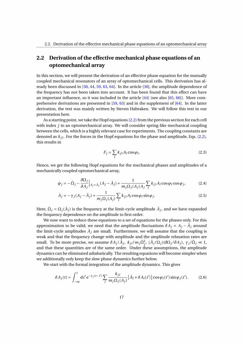
In this section, we will present the derivation of an effective phase equation for the mutuallycoupled mechanical resonators of an array of optomechanical cells. This derivation has al-ready been discussed in [30, 44, 59, 63, 64]. In the article [30], the amplitude dependence ofthe frequency has not been taken into account. It has been found that this effect can havean important influence, so it was included in the article [44] (see also [65, 66]). More com-prehensive derivations are presented in [59, 63] and in the supplement of [64]. In the latterderivation, the text was mainly written by Steven Habraken. We will follow this text in ourpresentation here.

As a starting point, we take the Hopf equations (2.2) from the previous section for each cellwith index j in an optomechanical array. We will consider spring-like mechanical couplingbetween the cells, which is a highly relevant case for experiments. The coupling constants aredenoted as k j l . For the forces in the Hopf equations for the phase and amplitude, Eqs. (2.2),this results in

F j =∑

lk j l Al cosϕl . (2.3)

Hence, we get the following Hopf equations for the mechanical phases and amplitudes of amechanically coupled optomechanical array,

ϕ j = − Ω j −∂Ω j

∂A j

∣∣∣A j=A j(A j − A j )+ 1

m jΩ j (A j )A j

∑l

k j l Al cosϕl cosϕ j , (2.4)

A j = −γ j (A j − A j )+ 1

m jΩ j (A j )

∑l

k j l Al cosϕl sinϕ j . (2.5)

Here, Ω j = Ω j (A j ) is the frequency at the limit-cycle amplitude A j , and we have expandedthe frequency dependence on the amplitude to first order.

We now want to reduce these equations to a set of equations for the phases only. For thisapproximation to be valid, we need that the amplitude fluctuations δA j = A j − A j aroundthe limit-cycle amplitudes A j are small. Furthermore, we will assume that the coupling isweak and that the frequency change with amplitude and the amplitude relaxation rates aresmall. To be more precise, we assume δA j /A j , k j l /m j Ω

2j , (A j /Ω j )(∂Ω j /∂A j ), γ j /Ω j ¿ 1,

and that these quantities are of the same order. Under these assumptions, the amplitudedynamics can be eliminated adiabatically. The resulting equations will become simpler whenwe additionally only keep the slow phase dynamics further below.

We start with the formal integration of the amplitude dynamics. This gives

δA j (t ) =ˆ t

−∞dt ′ e−γ j (t−t ′) ∑

l

k j l

m jΩ j (A j )

[Al +δAl (t ′)

]cosϕl (t ′)sinϕ j (t ′). (2.6)

17


It can be checked that this result solves Eq. (2.5) if it is reformulated in terms of the ampli-tude fluctuations. As a next step, we want to solve the integral in the equation above. Sincethe coupling only has a small influence on the phase dynamics, and because the amplitudedamping is smaller than the frequencies of the mechanical oscillations, we can replace thetime evolution of the phases in the integrand by the approximationϕ j (t ′) ≈ϕ j (t )−Ω j (t − t ′).Besides, we can neglect the second-order term containing k j lδAl . This results in the integral

δA j (t ) ≈ ∑l

k j l Al

m jΩ j (A j )

ˆ t

−∞dt ′ e−γ j (t−t ′) cos

[ϕl (t )−Ωl (t − t ′)

]sin

[ϕ j (t )−Ω j (t − t ′)

], (2.7)

which can be solved analytically. If we additionally assume that the frequency differences be-tween the oscillators are small,Ωl −Ω j ¿ γ j , we get the result for the amplitude fluctuations,

δA j ≈∑

l

k j l Al

m jΩ j (A j )

sin(ϕ j −ϕl )

2γ j, (2.8)

where we have also neglected fast oscillating terms.To make use of this result, we first rewrite the equations of motion of the phases, Eq. (2.4),

in terms of the amplitude fluctuations,

ϕ j ≈ −Ω j (A j )− ∂Ω j

∂A j

∣∣∣A j=A jδA j + 1

m jΩ j (A j )

∑l

k j l cosϕl cosϕ jAl

A j

(1+ δAl

Al− δA j

A j

). (2.9)

Now we insert the result for the amplitude fluctuations and keep only terms up to secondorder in the small parameters. In addition, we only keep slowly varying contributions byapproximating cosϕl cosϕ j ≈ 1

2 cos(ϕl −ϕ j ), cosϕl cosϕ j sin(ϕ j −ϕm) ≈ 14

sin(ϕl −ϕm)−

sin(ϕl +ϕm −2ϕ j ), and cosϕl cosϕ j sin(ϕl −ϕm) ≈ 1

4

sin(2ϕl −ϕ j −ϕm)−sin(ϕm −ϕ j )

. To

be consistent, we also have to consider the amplitude dependence of the frequency in thedenominator. However, this dependence would, overall, only produce higher order terms, sowe are left with the frequency at the steady state amplitude in the denominator. At last, weget

ϕ j = − Ω j +∂Ω j

∂A j

∣∣∣A j=A j

∑l

k j l Al

2γ j m j Ω jsin(ϕl −ϕ j )+∑

l

k j l Al

2m j Ω j A jcos(ϕl −ϕ j ) (2.10)

+∑l

∑m

k j l klm Al Am

8γ j m j Ω j A j ml Ωl Al

[sin(2ϕl −ϕm −ϕ j )− sin(ϕm −ϕ j )

]+∑

l

∑m

k j l k j m Al Am

8γ j m2j Ω

2j A2

j

sin(ϕm +ϕl −2ϕ j ).

This model will be called the general Hopf-Kuramoto model in the remainder of this thesis.The very general form given here still includes disorder in the parameters.

18

2.3. Previous results for the Hopf-Kuramoto model

In the following, we will assume that all oscillators are identical, so we can drop all indicesof the parameters, and that they are only coupled to their nearest neighbors, so k j l = k fornearest neighbors, and k j l = 0 for all other pairs. This reduces the sums to only run overnearest neighbor pairs, e.g. ⟨l , j ⟩. Furthermore, we absorb a trivial time evolution into thedefinition of the phase, ϕ j + Ωt →ϕ j . We define the parameters

C = k

2mΩ,

S1 = C A

γ

∂Ω

∂A

∣∣∣A=A , (2.11)

S2 = C 2

2γ.

This simplifies Eq. (2.10) to

ϕ j =C∑⟨l , j ⟩

cos(ϕl −ϕ j )+S1∑⟨l , j ⟩

sin(ϕl −ϕ j ) (2.12)

+S2

∑⟨l , j ⟩

∑⟨m,l⟩


]+ ∑⟨l , j ⟩

∑⟨m, j ⟩

sin(ϕm +ϕl −2ϕ j )

.

This model is what we call the Hopf-Kuramoto model. As we have seen in the derivation,it allows us to model the collective slow phase dynamics of coupled self-sustained oscilla-tors close to their individual limit cycles. Note that it only contains two parameters, namelythe ratios S1/C and S2/C . This makes it possible to cover a large portion of the parame-ter space with numerical simulations. Moreover, the coupling between the phases is onlythrough trigonometric functions of their phase differences. This simplicity allows some ana-lytical treatment in certain limiting cases, as we will see later. Besides, we can now relate thephysics of self-sustained optomechanical oscillators to other systems described by effectivephase equations. This will be discussed in the next chapter.

The Hopf-Kuramoto model is the main subject of interest in this thesis. We will presentresults about the pattern formation in one- and two-dimensional arrays in chapter 4. If theoptomechanical cells are subject to noise, for example laser shot noise, this can be modeledby complementing the right hand side of the Hopf-Kuramoto model with an additive noiseterm. This leads to interesting new effects, which will be discussed in chapter 5. These chap-ters will focus on effects in large arrays with local coupling. In the following section, we willpresent what is already known about the Hopf-Kuramoto model especially for small arraysand for global coupling.

2.3 Previous results for the Hopf-Kuramoto model

The general Hopf-Kuramoto model, Eq. (2.10), has been used for the study of optomechanicalsystems in the articles [30, 44]. Here, we want to review the most important results of thesepublications. More details can be found in [59, 63].

19


When the Hopf-Kuramoto model was introduced in [30], the change of the frequency withamplitude was not taken into account. This amounts to setting ∂Ω j /∂A j = 0 in Eq. (2.10) (orS1 = 0 in Eq. (2.12)). We will discuss now how the resulting model was then used to study thesynchronization of two dissimilar oscillators, which differ only in their natural frequencies.The frequency difference is denoted as δΩ = Ω2 −Ω1. This leads to the equation of motionfor the phase difference δϕ=ϕ2 −ϕ1,

δϕ= −δΩ− kδΩ

2mΩ2Ω1cosδϕ− k2(Ω2 + Ω1)2

8γm2Ω22Ω

21

sin2δϕ. (2.13)

If the frequency difference is small, δΩ¿ k/γm, the cosine term can be neglected and theequation is simplified further. It can then be seen that for sufficiently large coupling strength,the equation above has stationary solutions, δϕ = 0. This means that the phase differencebetween the oscillators stays fixed, the oscillators are strictly synchronized. In the limit dis-cussed here, the phase difference can either be close to 0 or π. This peculiar feature of bothin-phase and anti-phase synchronization can be traced back to the appearance of the factor2 in front of the phase difference in the equation above.

Those phenomena can be found in simulations of the microscopic optomechanical equa-tions of motion (see Eqs. (1.4)) for two coupled cells if the parameters are chosen correctly[30]. For sufficient coupling strength, the oscillators synchronize and the phase differencelocks to values close to 0 or π. Which of the two values is reached depends on the parametervalues and the initial conditions. To get a quantitative agreement between the microscopicsimulations and the effective phase model (2.13), in general the amplitude damping rate γhas to be kept as an adjustable parameter. Even if it is determined numerically from sim-ulations of single cells close to their limit cycle, the resulting value usually does not lead toconsistent results for coupled cells. This is explained in detail in [59]. The effective phasemodel fails to predict the behavior of coupled optomechanical cells in a regime where thereare large amplitude fluctuations. For the case of two cells, this happens in particular for largefrequency mismatch, δΩ> γ.

Also globally coupled arrays of optomechanical cells were studied before [30]. This kindof coupling can be realized with an extended optical mode with a large decay rate (κÀΩ j ).In numerical simulations of ten coupled optomechanical cells, it was found that for smallcoupling to the optical mode, the mechanical modes oscillate incoherently. This is reflectedin the fact that the order parameter χ = ⟨|N−1 ∑

j eiϕ j |2⟩ assumes values around 1/N , as itwould also be the case for uncoupled oscillators. Above a certain coupling strength, the orderparameter decreases because the coupling leads to anticorrelations in the phases. When thecoupling is increased even further, χ suddenly jumps to values close to one, indicating phaselocking with nearly identical phases. These features can also be found in simulations of theeffective phase model, Eq. (2.10) (again, with ∂Ω j /∂A j = 0 ). To get quantitative agreement,however, the parameter γ has to be used as a fit parameter, as it was the case for two coupledcells.

20

2.3. Previous results for the Hopf-Kuramoto model

The effective phase model was also used to study the influence of quantum noise on themany-body dynamics in optomechanical arrays, see [44]. First, semiclassical Langevin equa-tions for the mechanical mode and the optical mode were integrated on a two-dimensionallattice, for example with size 30×30. These equations contained an effective noise term witha fixed strength, given by the influence of quantum noise. As a result, for strong coupling thecorrelations decayed very slowly with distance. For weak coupling, however, the correlationsshowed a fast decay to zero. The transition from one behavior to the other happens very fastwith decreasing coupling strength. This is reflected in a rapid drop of the correlations for afixed distance when the coupling strength is changed.

This behavior was then compared to simulations of the effective phase model on a mean-field level. The mean-field equation of motion can be derived from the effective phase equa-tion (2.10) in a similar manner as for the Kuramoto model, see section 3.1. It is found thateach phase couples to the mean field Z = N−1 ∑

j eiϕ j , which in turn is determined by thephase values. In the presence of noise, the simulations reach a steady state, in which thecorrelations are evaluated. Qualitatively, the same results as for the Langevin equations areobtained: The correlations between two arbitrary phases show a rapid decrease for decreas-ing coupling strength around some “critical” value Kc. However, this value is underestimatedin the mean-field treatment. This is because the coupling appears to be stronger in the mean-field case than it is in the underlying, low-dimensional lattice model, where each cell is onlycoupled to a small number of nearest neighbors.

As we have seen in this section, the focus in the articles mentioned above was on thecomparison of the effective phase model to simulations of more microscopic equations ofmotion. In particular, synchronization of two coupled cells, in a globally coupled array andin a two-dimensional array subject to noise were studied in detail. It was found that theeffective phase model allows us to understand qualitatively many phenomena that appearfor coupled optomechanical cells. Furthermore, a close connection to the Kuramoto modelwas recognized. This model and some other relevant phase models will be reviewed in thenext chapter. This will set the stage for the further investigation of the Hopf-Kuramoto model,Eq. (2.12), which is the main topic of this thesis.

21

Chapter 3

Relation to models of nonlineardynamics and statistical physics

In this chapter, we will discuss some models which are closely related to the Hopf-Kuramotomodel. These models have been studied intensely in the past. We will present the aspectswhich are most important for the analysis of the Hopf-Kuramoto model in the following chap-ters of this thesis.

We will start with the classical Kuramoto model in section 3.1, describing synchronizationin an ensemble of globally coupled oscillators. In section 3.2, we will turn to the Kuramoto-Sakaguchi model with local coupling, where interesting pattern formation can be observed.Finally, in section 3.3, we will analyze a stochastic model, the XY model. This is particularly in-teresting because it shows a quasi-phase transition, the Kosterlitz-Thouless transition, whenthe noise strength is varied.

3.1 The Kuramoto model and synchronization

In 1975, Yoshiki Kuramoto proposed the following model to describe the phase dynamics ofN mutually coupled self-sustained oscillators [2],

ϕ j (t ) =ω j + S

N

N∑k=1

sin(ϕk −ϕ j ). (3.1)

This model is nowadays known as the Kuramoto model. A review of the research about thisand related models is given in [3]. In Eq. (3.1), we see that the oscillators have different nat-ural frequencies ω j and are all coupled to each other with the same coupling strength S/N .This kind of coupling is called global coupling. The coupling strength is scaled with the totalnumber of oscillators N in order to get reasonable results also in the thermodynamic limitN →∞. In this limit, the natural frequencies can be considered to be distributed accordingto some probability distribution g (ω j ).

23

Chapter 3. Relation to models of nonlinear dynamics and statistical physics

The coupling via the sine of the phase differences also shows up in one of the terms in theHopf-Kuramoto model, Eq. (2.12). Hence, it is instructive to study the effects of such a cou-pling. In particular, we are interested in the phenomenon of synchronization. We considertwo oscillators to be synchronized when their average frequencies Ω j (t ) are the same (or atleast very close to each other). The averaging is done over some time interval τ,

Ω j (t ) = 1

τ

ˆ t

t−τdt ′ϕ j (t ′). (3.2)

It turns out that for typical natural frequency distributions in the globally coupled Kuramotomodel, if there are synchronized oscillators, many of them have a similar phase (when takenmodulo 2π). Thus, it is helpful to study the behavior of the complex order parameter (ormean field)

Z =Reiψ = 1

N

N∑j=1

eiϕ j . (3.3)

This equation defines the real-valued, non-negative phase coherence R and the mean fieldphase ψ. A finite value of R hints at the coherence of some oscillators. It is possible to com-pute this quantity analytically for some special distributions g (ω j ), in the limit N →∞. Wewill explain the procedure in the following. For more details, see [1].

First, the equation of motion, Eq. (3.1), is rewritten with the help of the mean field,

ϕ j =ω j +SR sin(ψ−ϕ j ). (3.4)

We see that each oscillator is coupled to the mean field in the same way. This equation has tobe solved self-consistently together with Eq. (3.3).

Under the assumption that the mean field oscillates regularly with a constant amplitudeand a single frequency, it is found that there can be two groups of oscillators: One group,whose natural frequencies are close to the mean-field frequency, will synchronize to this fre-quency. The other group, with natural frequencies differing significantly from the mean-fieldfrequency, will not synchronize and oscillate incoherently. The contributions of both groupsto the mean field can be calculated. This gives an equation for the phase coherence R, whichcan be solved for some special natural frequency distributions.

One of those solvable cases is the Lorentzian distribution, with width γ and centeredaround zero,

g (ω j ) = 1

πγ(1+ω2

j /γ2) . (3.5)

In this case, there is a critical coupling strength Scrit = 2γ. For values of S below that threshold,the ratio of synchronized oscillators vanishes and the mean field is zero (and therefore alsothe phase coherence R). Above threshold, there are many synchronized oscillators. Their

24

3.1. The Kuramoto model and synchronization

ttime

phas

e '

j(t

)

0 10 20 0

10

20

2

0 10 200.0

0.5

1.0

0 20

0.5

R

coupling strength S/

phas

e co

here

nce

R

critical coupling strength

0 2 40.0

0.5

1.0

200 400−5

0

5

200 400 0

2

4

6

0

2

oscillator index j

effec

tive

frequ

.j/S

phas

em

od '

j(t

)2

synchronized oscillators

a b c

Figure 3.1: Synchronization in the Kuramoto model. (a) Initial time evolution of selectedphases in a simulation with 500 oscillators. It can be seen that after some time, two of theoscillators (blue and cyan curves) synchronize, while the other two (magenta and red curves)evolve with higher frequencies. For very short times, all oscillators evolve with their naturalfrequencies (dotted lines). The inset shows the build-up of the phase coherence R. The nat-ural frequencies were picked from a Lorentzian distribution and the coupling strength wasS/γ = 3. (b) Characteristics of the synchronized state at γt ≈ 300. A lot of oscillators havethe same effective frequency (top). Hence, those are all synchronized. The phases of the syn-chronized oscillators, when taken modulo 2π, are very similar (bottom). This leads to a finitephase coherence R. The oscillators are sorted by their natural frequencies and the ones from(a) are marked with colored crosses. (c) Dependence of the phase coherence R on the cou-pling strength. The analytical solution for infinitely many oscillators (red curve) predicts afinite value above a critical coupling strength Scrit = 2γ. The simulations with 500 oscillatorsup to time γt = 300 (black markers) agree qualitatively, but show finite-size and finite-timedeviations. The blue circle marks the simulation discussed in (a) and (b).

phase differences will actually be small. This leads to a finite phase coherence. The analyticalsolution is

R =√

1− 2γ

S, S > Scrit = 2γ. (3.6)

All the features discussed above can also be seen in simulations of Eq. (3.1). In Fig. 3.1, weshow results of simulations with 500 oscillators and random initial conditions. In Fig. 3.1a,where the coupling strength is chosen to be above threshold, we see that after initial tran-sients, some oscillators synchronize. On the same timescale, the phase coherence R buildsup (see inset).

In the top panel of Fig. 3.1b, we show the effective frequencies of the oscillators after atotal simulation time ofγt = 300. The oscillators are sorted by their natural frequencies on thehorizontal axis. We find that a lot of oscillators have the same effective frequency. Let us stress

25


that this is the characteristic feature of synchronization. The synchronization frequency isclose to zero, which is the center of the distribution from which the natural frequencies weredrawn. We computed the effective frequencies by averaging over the second half of the totalsimulation time.

The bottom panel shows a snapshot of the phase field, taken modulo 2π, close to the endof the simulation. We see that the synchronized oscillators have a very regular phase relation:The phase differences are small for oscillators with similar natural frequencies, while theybecome larger for an increasing mismatch. The unsynchronized oscillators with very smalland very large natural frequencies have no regular phase structure.

Finally, in Fig. 3.1c, we plot the phase coherence R at the end of simulations with differentcoupling strength S/γ. We see that the numerical results, which are shown by black markers,agree qualitatively with the red line of the analytical result, which was given in Eq. (3.6). How-ever, we also see deviations because of the limited simulation time and the finite number ofoscillators.

In conclusion, we have seen in this section that the Kuramoto-like coupling of oscillatorswith different natural frequencies can make them synchronize, i.e. agree on a common effec-tive average frequency. In particular, the Kuramoto model can be solved analytically for somefrequency distributions. For the Lorentzian distribution, it shows a simultaneous appearanceof synchronization and a finite phase coherence above a critical coupling strength.

We remark that the latter does not happen in general. There could be frequency distribu-tions where phase coherence appears without synchronization, or the other way around. Inthe next section, we will actually see that in a similar model, a perfectly synchronized systemcan have a vanishing phase coherence.

3.2 The Kuramoto-Sakaguchi model and pattern formation

The Kuramoto model, which was discussed in the previous section, captures many importantfeatures of synchronization. However, it can not reproduce the behavior of some cells inliving systems, which oscillate faster when they are coupled to each other than when they areisolated. With that in mind, H. Sakaguchi and Y. Kuramoto proposed to introduce a phase lagα into the coupling function [67, 68] (see also Eq. (2.34) in [69]),

ϕ j (t ) =ω j + K

N

N∑k=1

sin(ϕk −ϕ j +α). (3.7)

This model is called Kuramoto-Sakaguchi model. Later it was argued that it actually describesthe phase dynamics of an array of Josephson junctions [70].

For the globally coupled system as described by Eq. (3.7), a study similar to the one in theoriginal Kuramoto model, which was described in the previous section, can be conducted. Atleast for sufficiently small values of the phase lagα, a transition from an unsynchronized (andincoherent) regime to a synchronized regime (with finite phase coherence) can be found [67].

26

3.2. The Kuramoto-Sakaguchi model and pattern formation

The relevant parameter is again the ratio of the coupling strength to the width of the naturalfrequency distribution.

The Kuramoto-Sakaguchi model is very important for our study of the Hopf-Kuramotomodel, Eq. (2.12), because it contains the sine and the cosine coupling functions. This can beseen when we use C /S1 = tan(α) and S2

1+C 2 = K 2. When we additionally restrict the couplingto include only the nearest neighbors, we get

ϕ j (t ) =ω j +C∑⟨k, j ⟩

cos(ϕk −ϕ j )+S1∑⟨k, j ⟩

sin(ϕk −ϕ j ). (3.8)

The model with this local coupling was already studied in [68]. It was observed that phasepatterns form, particularly in two-dimensional lattices.

Pattern formation is an interesting phenomenon, which has been studied intensely, seethe review article [4]. Usually, as in our case, one studies a set of deterministic nonlinear (par-tial) differential equations. To be more precise: “An aim of theory is to describe solutions ofthe deterministic equations that are likely to be reached starting from typical initial condi-tions and to persist at long times” [4]. In this spirit, we will now discuss the most prominentexamples of patterns in the two-dimensional Kuramoto-Sakaguchi model.

In the simplest case, where the disorder in natural frequencies is not too drastic, and theparameter C (or correspondingly,α) is not too large, the system will always reach a stationarystate. With this expression we mean that the phase velocities of all sites are equal: ϕ j = ϕk forall pairs j ,k. However, the phase relations between the oscillators can be non-trivial and willlead to the patterns mentioned above.

We want to start by discussing target patterns, see Fig. 3.2a and b. Those are patternswhere the phase increases (or decreases) linearly with the radial distance from some point,which is the target center. These patterns usually form when a region that has a significantlydifferent frequency from the rest of the array entrains the whole array. It depends on themodel parameters whether a slower or a faster region can entrain the rest of the array. In ourexample of Fig. 3.2a, where we used positive parameters S1 and C , the central 25 oscillators(forming a 5×5 square) have a lower natural frequency, which leads to the formation of thetarget pattern.

The mechanism of this formation can be understood by a continuum approximation ofthe full phase equation for a homogeneous system with small phase differences. The sloweroscillators are then modeled as a defect on that background, see [71]. Roughly speaking, inthe homogeneous medium the phase equation allows waves with arbitrary wavelength. Onlythe phase velocity will be determined by the wavelength. However, if there are defects, thosewill pick out a special wavelength λ, which depends on the microscopic details of the defects.These details might be too complicated to allow a full analytical treatment. Nevertheless, onecan still write down a relation between the selected wavelength λ and the phase velocity in

27


jxlattice coordinate

j yla

ttice

coo

rdin

ate

a b c

0 2

00

400

600

800

1000

0

200

400

600

800

1000 0

2

'j

Figure 3.2: Pattern formation in the Kuramoto-Sakaguchi model, Eq. (3.8). We show exam-ples of stationary patterns for different natural frequency distributions and different initialconditions. (a) A target pattern. The central 25 oscillators have natural frequencies which arelower by 0.8C than the ones in the rest of the array. All oscillators have agreed on a commoneffective frequency. This is possible due to the formation of the target pattern with linearlyincreasing phases in radial direction from the center. (b) A target pattern in a system with dis-ordered frequencies (equally distributed in an interval of width 3.7C ). Because of the disor-der, the pattern is not perfectly symmetric. Still, a stationary state can be reached by formingthis stable pattern. In (a) and (b), the lattice size was N = 1282 and the phases were initiallyequal. (c) An extended spiral in a system without frequency distribution. As initial condi-tions, we chose a vortex phase pattern. Its center was at the place where we see the spiralcenter in the figure. Initially, the phase contour lines stretched outwards radially. In the timeevolution, the phase contour lines wound up into the stable spiral configuration. The latticesize was N = 2562 and we only show a part of the phase field. In all simulations, S1/C = 1.8,and periodic boundary conditions were used. Patterns similar to the ones presented here arealso shown in [68].

the stationary state:

ϕ j =2C[

1+cos(2π

λ

)]≈4C

(1− π2

λ2

), (3.9)

where the last approximation is valid for large wavelength, λÀ 2π. This equation again em-phasizes the remarkable fact that the frequency of the whole array is determined by the pres-ence of a single defect, which forms the target center. Therefore, this is called the pacemakerof the array.

Pacemakers can also be present in systems without frequency distributions if there arelarge phase differences. Usually, those differences will vanish with time. However, there is aconfiguration where this is not possible for topological reasons. This is the vortex. Its char-acteristic feature is that the phase changes by 2π when one goes around the vortex center in

28

3.2. The Kuramoto-Sakaguchi model and pattern formation

a closed loop. On the square lattice, this means that there are phase differences as large asπ/2 between nearest neighbors. For vanishing parameter C , a vortex with radially outgoingphase contour lines is dynamically stable. This already leads to interesting effects when noiseis added, as we will see in the next section.

Here, we want to focus on the case of a finite value of the parameter C . Then, the largephase differences lead to a very different phase velocity at the vortex center as compared tothe rest of the lattice. As a consequence, the phase contour lines will bend until a perfectspiral is formed, see Fig. 3.2c. As in the case of target patterns, a small pacemaker region,which is the spiral center here, has entrained the whole lattice. The resulting phase velocity isdirectly related to the spiral arm width λ, and the relation is given by Eq. (3.9). The propertiesof spirals and their wavelength in systems without frequency distribution will be discussed indetail in section 4.1.1.

Let us point out that also in randomly disordered systems, the patterns that have beendiscussed so far can show up. Fig. 3.2b shows the final, stationary state of a simulation withequally distributed natural frequencies, started from homogeneous initial conditions. Wecan see that there is a target pattern, which is distorted because of the disorder. For differentparameters, there can also be rudimentary spirals. This is not shown here.

Both the stationary targets and the stationary spirals are examples of perfectly synchro-nized systems. However, because all phase values appear equally often in the array, the Ku-ramoto order parameter from the previous section vanishes in these cases. Hence, it is notsuitable for signaling synchronization in the Kuramoto-Sakaguchi model with local coupling.

So far, we have only mentioned stationary patterns. But there can also be non-stationarypatterns, even when the oscillators are identical in their natural frequencies. These patternswill be discussed in the sections 4.1.1 and 4.2.2. The first of those sections will also include astudy of the properties of the rudimentary spirals mentioned above.

The discussion up to now might suggest that we deal with very special patterns here,which show up only in the Kuramoto-Sakaguchi model. However, models of many oscilla-tory systems actually lead to the same continuum approximation, which was used above forthe motivation of the existence of targets and spirals. Hence, this explanation gives an answerto the question why these patterns arise in many physical, chemical and biological systems[4]. Furthermore, the stability of the patterns has to be studied. For example, there could alsobe spirals with multiple arms in the Kuramoto-Sakaguchi model, where the phase changesby a multiple of 2π on a loop around the center. However, those spirals are not stable. Thisseems to be a general feature of spiral solutions in many pattern-forming systems [4].

To summarize, in this section we have discussed that the Kuramoto-Sakaguchi model,Eq. (3.7), is a very important extension of the original Kuramoto model. In particular, for lo-cal coupling (see Eq. (3.8)), it has interesting additional features. One of these is the abilityto form phase patterns. We have discussed target patterns and spirals, where a small re-gion of the oscillator array acts as a pacemaker and entrains the whole lattice. Especiallythe spirals will be very important for our detailed discussion of the pattern formation in theHopf-Kuramoto model in section 4.1.1.

29


3.3 The XY model and the Kosterlitz-Thouless transition

In the previous two sections, we have focused on the deterministic dynamics of nonlinearphase models. In this section, we want to discuss the stochastic dynamics in the so-called XYmodel [72, 73]. This model is similar to the Ising model because it describes the interactionof “spins” on a lattice, and where one is particularly interested in the effects of finite tem-perature. However, in the XY model the “spins” are considered to be classical and they arerestricted to rotation in a plane. Therefore, they are described by a single continuous phasevariable. Here, we focus on the simple case of nearest-neighbor interaction with identicalcoupling constants. Furthermore, we do not take into account external (“magnetic”) fields.Hence, the total energy of a phase configuration is given by

U = − J∑⟨k, j ⟩

cos(ϕk −ϕ j ), (3.10)

where the sum runs over all nearest-neighbor pairs on the lattice. For a positive value of thecoupling strength J , we can see that the system has a trivially degenerate set of ground states,in which all phases are equal.

At low temperatures, the energetically low-lying excitations with small nearest-neighborphase differences are particularly important. Those are called spin waves. Their effects can bestudied analytically by expanding the cosine in Eq. (3.10) up to second order. With the stan-dard methods of Statistical Mechanics, it can then be shown that in one- and two-dimensionallattices with N sites, the average “magnetization” in the system vanishes, ⟨|N−1 ∑N

j=1 eiϕ j |⟩ =0, in the thermodynamic limit N →∞. This is because there are no long-range correlations inthe system, as expected by the Mermin-Wagner-Hohenberg theorem [74, 75]. In one dimen-sion, it can be shown easily in the expanded model that the correlations decay exponentiallyfast with the distance, ⟨

exp[i (ϕk −ϕ j )

]⟩=exp(−|k − j |/Ξ)

, (3.11)

with a temperature-dependent correlation length Ξ = kBT /2J . Hence, the system only dis-plays short-range order. In two dimensions, the correlations decay with a power law for largedistances,

⟨exp[i (ϕk −ϕ j )]

⟩∼ ‖~rk−~r j‖−η, with a temperature-dependent exponent η [73, 76].The norm ‖~rk −~r j‖ denotes the geometrical distance of the sites k and j in two dimensions.The power-law decay is very slow. Hence, there is still some order left in the system, which isthen called quasi-long-range order.

At high temperatures, this order is destroyed and the correlations decay exponentiallyfast with the distance. The fact that there is a transition between the two regimes is veryremarkable. This transition is called a Kosterlitz-Thouless quasi-phase transition [72, 73, 77].One characteristic feature of this transition is that the correlation length diverges when thetransition temperature is approached from above, even though no true long-range order isestablished.

30

3.3. The XY model and the Kosterlitz-Thouless transition

So far, we have discussed the equilibrium properties of the XY model. In numerical stud-ies, very efficient Monte-Carlo methods are usually employed for simulations. However, it isalso possible to simulate the XY model by numerically integrating the equations of motion forthe individual phases ϕ j . For example, this also makes it possible to observe the transientsfrom an arbitrary initial state. We will focus on that approach now because it is much closer inspirit to the approach that we use to explore the (generally) non-equilibrium Hopf-Kuramotomodel.

We get the equations of motion by assuming that the phases perform an overdampedmotion in the (appropriately rescaled) potential U of Eq. (3.10), while they are also subject tothe influence of noise. Hence,

ϕ j = − S1

J

∂U

∂ϕ j+ξ j = S1

∑⟨k, j ⟩

sin(ϕk −ϕ j )+ξ j , (3.12)

with the noise correlator ⟨ξ j (t )ξk (0)⟩ = 2Dϕδ j kδ(t ). We see that we have recovered the cou-pling term of the Kuramoto model, which is also contained in the Kuramoto-Sakaguchi modeland the Hopf-Kuramoto model. This shows the close connection of the XY model to thosemodels.

In the simulations of Eq. (3.12), we can qualitatively observe the properties of the XYmodel that we have discussed above. However, finite size effects will always play an impor-tant role for weak noise [78]. We will discuss this now in more detail. After some simulationtime, the equilibrium state is reached, where the statistical properties of the phase field donot change any more and where they do not depend on the initial conditions. For very weaknoise, we can then see phase fields where all sites have similar values, see Fig. 3.3a. Note thatthis would not be the case for infinite system size because there is no true long-range order.For larger noise, we can see that the spatial fluctuations of the phases increase, see Fig. 3.3b.All phase values are present even in the finite system. Still, there are large domains of similarphase values. This changes drastically when the noise is increased beyond the Kosterlitz-Thouless transition noise strength, as depicted in Fig. 3.3c. The phase now changes quicklyin space.

The behavior discussed above is reflected in the dependence of the correlations in space,Re

⟨exp[i (ϕk −ϕ j )]

⟩, on the distance r = ‖~rk −~r j‖, see Fig. 3.3d. For weak noise, the corre-

lations decay slowly and fit well to the expected power-law behavior, see the top blue curve.For strong noise, the decay is exponentially fast, see the lowest red curve. In between thesetwo extreme regimes, the correlations can be fit well with a product of a power law decay andan exponential decay, as described in the figure caption.

In a finite-size system, the Kosterlitz-Thouless transition can be seen very clearly whenone analyzes the dependence of the correlation length (from the fits mentioned above) onthe noise strength, see Fig. 3.3e. When the noise strength is decreased, the correlation lengthincreases. It becomes larger than the system size at a finite noise strength. This value is thendefined to be the critical transition noise strength for a finite-size system, see [78]. In thisarticle, the authors find a critical value Dϕ/S1 ≈ 1.02 for a system of size N = 1002. We use

31


a b c

0 2

00

40

0 6

00

80

0 1

00

0 0

20

0

40

0

60

0

80

0

10

00 0

2

'j

noise strength D'/S1

corre

latio

n le

ngth

quas

i-lon

g-ra

nge

orde

r

shor

t-ran

ge o

rder

e

0.6 0.8 1.0 1.2 1.4 0

5

10

15

20

distance

corre

latio

nsR

ehe

xp[i('

k

'j)]i

dweak noise

strong noise

0 10 20 300.0

0.5

1.0

k~rk ~rjk

phase field

xy

Figure 3.3: The Kosterlitz-Thouless transition in the two-dimensional XY model. We show re-sults of simulations of Eq. (3.12) in systems of size N = 1002. (a)-(c) Plots of the phase field inthe equilibrium state for different noise strength, Dϕ/S1 = 0.3, 0.8, 1.2 (from left to right). (d)Decay of the correlations with distance for different noise strength, Dϕ/S1 = 0.1, 0.3, . . . , 1.5(from top to bottom). For weak noise, we only see a very slow decay. For strong noise, the cor-relations decay very fast. The data can be fit well with a combination of a power law decay andan exponential decay, f (r ) = exp(−r /Ξ)/(1+ r η), with distance r and fit parameters Ξ and η.(e) The correlation lengthΞ (from fits to the data) in dependence on the noise strength (blackmarkers). We can see that the correlation length increases for decreasing noise strength. It be-comes comparable to the system size for finite noise. This indicates the Kosterlitz-Thoulessquasi-phase transition from short-range order (red region) to quasi-long-range order (blueregion). For the definition of the transition noise strength, see the main text. Different datasets were used in the figures.

32

3.3. The XY model and the Kosterlitz-Thouless transition

this value for depicting the transition in Fig. 3.3e and see that our findings are consistent withthis result.

The mechanism behind the Kosterlitz-Thouless transition is the unbinding of vortices[73]: At low noise strength, vortices and antivortices are not present or they exist only inbound pairs. Therefore, they do not influence the correlations of the phase field on largescales. The important fluctuations are just the spin waves (with small nearest-neighbor phasedifferences), which were mentioned above and lead to a power-law decay of the correlations.For large noise, however, the vortices and antivortices can unbind. As a consequence, thepresence of free vortices scrambles the phase field drastically on large scales. This is why thecorrelations decay exponentially beyond the Kosterlitz-Thouless transition noise strength.

We will now explain how this critical value can be estimated. The energy of a single vortexcan be calculated approximately by expanding the cosine in Eq. (3.10) up to second order andgoing over to a continuum approximation,

U ≈ −2J N + J

2

∑⟨k, j ⟩

(ϕk −ϕ j )2 ∼ const.+ J

2

ˆd2r (∇ϕ)2,

U [ϕVortex] ∼const.+ Jπ lnR

a. (3.13)

To arrive at the result in the second line, we have inserted the phase field of a vortex in thecontinuum, ϕVortex(r,φ) = φ with polar angle φ. The constant on the right hand side of thesecond line contains energy contributions from the core, up to the core cutoff a, and R isthe system size. We see that the presence of a vortex increases the free energy of the system,F = U −T S, for low temperatures. However, a vortex also increases the entropy S becauseit can be located at any position in the system. Hence, for increasing temperature, the en-tropy contribution becomes more important. Eventually, the presence of a free vortex candecrease the free energy as compared to the homogeneous phase field. The temperaturevalue at which this happens gives the critical temperature. To arrive at a quantitative pre-diction, the interaction of many vortices and the contributions of the spin waves have to betaken into account. For a full discussion, see [73].

We conclude that vortices play a central role in the XY model. Their unbinding at a finitecritical temperature (or noise strength) is responsible for the Kosterlitz-Thouless transitionfrom a state with quasi-long-range order to a state with short-range order. This is an exampleof the interesting interplay between topological defects like vortices and the effects of noise.Note that we have studied the equilibrium state of the XY model. In chapter 5, we will studythe effects of noise in a non-equilibrium setting, the Hopf-Kuramoto model. Among otherthings, we will see that spirals take over the role of vortices and that this significantly changesthe physics.

33

Chapter 4

Deterministic dynamics and patternformation in the Hopf-Kuramotomodel

In the previous chapter, we have seen that phase-only models of coupled limit-cycle oscil-lators exhibit interesting phenomena like synchronization and pattern formation. In thischapter, we will explore those phenomena in the deterministic Hopf-Kuramoto model, Eq.(2.12). First, we will have a close look at pattern formation in large two-dimensional arrays.We will see that spirals play an important role. As a main result, we will derive a pattern phasediagram in the two-dimensional parameter space of the model in section 4.1.1. This diagramtells us which patterns are typically developed when starting from random initial conditions.We will also have a shorter look at pattern formation in one-dimensional arrays in section4.2.

After mainly reviewing the work of other researchers in the previous chapters, in this andthe following chapter we will present original work of the author of this thesis. The mainresults of section 4.1 have been published in a very similar form in

• Roland Lauter, Christian Brendel, Steven J. M. Habraken, and Florian Marquardt,Pattern phase diagram for two-dimensional arrays of coupled limit-cycle oscillators,Physical Review E 92, 012902 (2015)Copyright (2015) by the American Physical Society

Some minor details have been changed to ensure compatibility with this thesis. This includesthe removal of the general presentation of the Hopf-Kuramoto model because this was al-ready introduced in chapter 2. Besides, the detailed derivation of the Hopf-Kuramoto model,which was contained in the article mentioned above, was removed because it has alreadybeen discussed in section 2.2.

35

http://journals.aps.org/pre/abstract/10.1103/PhysRevE.92.012902

Chapter 4. Deterministic dynamics and pattern formation in the Hopf-Kuramoto model

4.1 Pattern phase diagram for two-dimensional arrays of coupledlimit-cycle oscillators

In the previous chapter, we have already discussed synchronization in the Kuramoto model.In general, synchronization is an important concept in many branches of physics, chemistry,biology and other sciences [1]. Considering physical systems, within the past three years, anumber of experiments have demonstrated for the first time synchronization between twonanomechanical oscillators [56, 57], two micromechanical oscillators [27], and in small ar-rays of the latter [58]. As it was discussed in detail for optomechanical systems in section 1.2,those systems are driven through a Hopf bifurcation into a limit-cycle oscillation, where theenergy pump is supplied through feedback or an optical drive. Future, large arrays of syn-chronized mechanical Hopf oscillators promise to provide robustness against both disorderand noise. Considerable theoretical attention has recently been devoted to the problem ofsynchronization in arrays, both on the general level and for predicting the behavior of spe-cific systems (e.g. in nanomechanics [30, 40, 65, 66, 79, 80] or trapped ion systems [81]). Someprogress has also been made in the quantum regime [44, 61, 82–84]. As we have already ex-plained in chapter 2, it is efficient to focus on the dynamics of the crucial phase degree offreedom, where the most prominent phenomenological model is the one introduced by Ku-ramoto (see section 3.1 and [2, 3]), which more recently has been supplemented by so-calledreactive terms [62, 66]. This leads to the Kuramoto-Sakaguchi model, which was presented insection 3.2.

Here, we will explore synchronization and deterministic pattern formation for a two-dimensional array of identical Hopf oscillators, as effectively described by the Hopf-Kuramotomodel, Eq. (2.12). This implies that the classical phase evolution is affected by extra contribu-tions beyond those investigated previously, for example in the Kuramoto-Sakaguchi model.These can have a significant impact on the dynamics. Our simulations of the effective modelreveal various stationary and non-stationary patterns in different parameter regimes. Phasecorrelators, length scales, and macroscopic pattern dynamics will be discussed in section4.1.1. These are relevant for determining whether an array can easily settle into a phase-locked state, which is important for applications.

There is already a sizeable literature on the rich nonlinear dynamics of pattern-formingsystems, including spiral dynamics (see [4, 85] and references therein). The main point of thissection is the investigation of a model which will be of importance because it arises generi-cally for coupled limit-cycle (Hopf) oscillators. This comprises a large class of physical sys-tems, including those studied in the context of the synchronization dynamics of opto- andnanomechanical oscillators.

In the future, one could couple many of those optomechanical oscillators to build largeoptomechanical arrays, see [30, 44, 45, 48, 86] and section 1.3. The properties of these deviceshave been investigated theoretically recently, both for global coupling [40–42, 47, 87] andlocal coupling [43, 46, 49, 50, 53]. Pattern formation in the mechanical phases can only beobserved for locally coupled oscillators, which would show up naturally in optomechanical

36

4.1. Pattern phase diagram for two-dimensional arrays of coupled limit-cycle oscillators

crystals [18, 88, 89]. In section 4.1.2, we will describe optomechanical arrays in more detailand discuss their relevance as a setup for the experimental implementation of coupled limit-cycle oscillators.

Our aim is to explore the dynamics of the Hopf-Kuramoto model on a square lattice. Westart with the discussion of some of the terms of this model. As we have seen in the last chap-ter, the term sin(ϕl −ϕ j ) of Eq. (2.12) is well known from the Kuramoto model [2], or, equiva-lently, the XY model [73]. In the Hopf-Kuramoto model, the term arises from the amplitude-dependence of the frequency [65], see section 2.2. Both contributions in the first line of Eq.(2.12) have been derived previously for coupled limit-cycle oscillators, see [62]. They are lin-ear in the coupling k, see Eqs. (2.11). In contrast, the prefactor S2 is of second order in k.However, as discussed in section 4.1.2, in realistic scenarios γ and ∂Ω/∂A can become small,such that the regime with S2 ∼ S1 and S2 ∼ C is easily reached. The S2-term can then havea profound influence on the pattern formation dynamics. The additional contribution alsodisplays next-to-nearest-neighbor coupling of the phases, in spite of the underlying intrinsicnearest-neighbor coupling in the lattice assumed here. With the exception of [30, 44] (wherepattern formation was not considered), the S2-term has not been discussed previously in theliterature on models for the effective phase dynamics of coupled limit-cycle oscillators, to thebest of our knowledge.

We will first set the stage by highlighting several limiting cases of our model, some ofwhich are known already. For C = 0, Eq. (2.12) can be rewritten in the form ϕ j = −∂U /∂ϕ j .Hence, the system will slide down to a minimum of the potential U . In contrast, for non-vanishing C , such a potential does not exist and the system may never reach a stationary state(where ϕ j is constant). The limiting case of Eq. (2.12) with S2 = 0 is the Kuramoto-Sakaguchimodel (see section 3.2).

The continuum limit of Eq. (2.12), which is valid for smooth phase fields, is given by

ϕ=S1∆ϕ−2S2∆2ϕ−C (∇ϕ)2 +4C , (4.1)

where S1 = S1a2, S2 = S2a4, C =C a2, with lattice constant a, and ∆ is the Laplace operator.In this model (with S2 = 0) it has been found that spirals can develop around singularities inthe phase field [69, 71]. Besides, it has been analyzed in connection with chemical turbulencein one dimension [90–92].

4.1.1 Pattern formation

The aim of this section is to explore pattern formation in the full model, Eq. (2.12), in largetwo-dimensional arrays. Our main result is the pattern phase diagram discussed further be-low. The patterns we find will determine the phase synchronization dynamics of limit-cycleoscillators.

Our numerical results are mostly obtained from simulations with a random initial phasefield, since that is the natural starting point in real systems (e.g. after switching on the pump

37


c) d)

plots of the phase field are for S_1/C=2.0

0.0.

1.5 2.0

5

10

15

S1/C

correlation minimaspiral arm width

stationary

statio

nary

non-stationary

non-stationary

0 2

00

40

0 6

00

80

0 1

00

0 0

20

0

40

0

60

0

80

0

10

00 0

2

'i

d

distancecorre

latio

nsR

ehe

i('

m'

n)i

S1/C = 1.70

S1/C = 1.60

0 10 20

−0.1

0.0

0.1

0.2

|~rm ~rn|

phase field

xy

0.0.

0.0.

Figure 1

c

a b

Figure 4.1: Spiral patterns and length scales in the Hopf-Kuramoto model. (a) Stationaryspiral pattern emerging from random initial conditions for S1/C = 2.0, S2/C = 0 on a N ×Nsquare lattice (N = 128) with periodic boundary conditions. (b) Vortex-anti-vortex pair (seeinset) winding up to a stationary spiral-anti-spiral pair with a characteristic spiral arm widthλ. Parameters are like in (a). (c) Spatial correlations Re⟨exp(i (ϕm −ϕn))⟩ as a function of thedistance |~rm −~rn | (rounded to the nearest integer). To obtain the data for (d), we extract thefirst correlation minimum position from parabolic fits and average over 10 runs with differentrandom initial conditions. (d) The location of the first correlation minimum (red) and thespiral arm width λ from (b) (black), as a function of the ratio S1/C , in units of the latticeconstant. There can be hysteresis (blue). (This figure has previously been published in [64].)

38


laser or the feedback driving the oscillators into the limit cycle). After some transient dynam-ics, we often find patterns that do not change qualitatively any more on longer time scales.Moreover, in certain parameter regimes, we find nontrivial stationary patterns.

A typical final pattern of a simulation with large S1/C is shown in Fig. 4.1a. This patternis stationary. It consists of many vortex-like “singularities”, where the phase changes by 2πwhen going around in a closed loop. These points are surrounded by spiral structures. Spiralpatterns in general are well-known as a recurring motif in pattern formation, see [4, 85, 93]and section 3.2. Since they form an important part of the patterns we observe, we now brieflydiscuss the properties of isolated spirals (see Fig. 4.1b) produced from an initial conditionwith a vortex in the phase field (shown in the inset).

It is known that in related models, there is a transition from stationary spirals to non-stationary spirals, i.e. a situation when the spiral centers are no longer phase-locked to thebulk of the lattice [68, 94]. We have discovered that this transition also gives rise to a jump inthe width of the spiral arms, λ (Fig. 4.1d). Outside of the jump, λ increases with increasingS2/C and S1/C (black curve in Fig. 4.1d). When sweeping the parameter ratio S1/C up anddown, we find hysteresis in the spiral arm width (blue line in Fig. 4.1d). The precise value atwhich the jump occurs can then depend on the parameter sweep rate. Our analysis illustratesthat the microscopic details of the spiral center, on the scale of a few lattice sites, influenceboth the spiral arm width and the macroscopic pattern considerably. Because the structureof the spiral core is complicated, we cannot provide an analytical prediction for λ.

We now turn to the statistical properties of the patterns which evolve out of random initialconditions (see Fig. 4.1a), as they are directly relevant for experiments. The spatial correla-tions of the phase field are characterized by the correlator ⟨exp(i (ϕm −ϕn))⟩, whose distancedependence is displayed in Fig. 4.1c. We find an oscillatory structure connected to the pres-ence of spiral arms. On top of that, there is an exponential decay, due to the presence ofmany randomly located spiral centers. The position of the first minimum in the oscillationsindicates the distance approximately set by half a spiral arm width. The dependence of thisposition on the parameter S1/C is shown as the red line in Fig. 4.1d. Again, we find a suddenjump associated with the transition from stationary to non-stationary spiral centers. We notethat the spiral arm width λ determined for isolated spirals does not agree completely withthe length scale extracted from the oscillations of the correlator. The difference can be tracedback to changes in the spiral core produced by the presence of other nearby spirals.

There are only two dimensionless parameters, S1/C and S2/C , that determine the prop-erties of the final pattern. Therefore, a complete overview of the various regimes in our modelis provided by the “pattern phase diagram” in Fig. 4.2. This summarizes the main results ofour studies in this section, and we now explain its features. For more details about the con-struction of this diagram, see the appendix A.1.

The transition discussed above, between stationary and non-stationary spirals, is sharpand can be traced up to intermediate values of S2/C . In addition, we find two classes of non-stationary spirals: “pulsating” spirals, where the core keeps orbiting in a small circle arounda fixed location [94], and truly mobile spirals that move through the whole lattice. We will

39


0.01 0.1 1.0 10.0

1.0

10.0

2.

0.5

5.5

10

2

1

0.5

stationary spirals

pulsating spirals

spirals and -defects

vortices

“fluctuating” patterns

mobile spirals

“complex” patterns

S1/C

stationary

1010.10.01

a

b

c

d

e

f

S2/C

non-stationary0.01 0.1 1.0 10.0

1.0

10.0

2.

0.5

5.

a

b

c

d

e

f

Figure 4.2: Pattern phase diagram of the Hopf-Kuramoto model, Eq. (2.12). Different colorsindicate different patterns, which are discussed in the main text. Sharp transitions occur be-tween stationary spirals and pulsating/mobile spirals (for small S2/C ), and in the appearanceof “π-defects”. Point markers indicate parameters explored by numerical simulation. Sometypical phase patterns are shown in the insets (a) to (f). (This figure has previously been pub-lished in [64].)

comment on their dynamics later. We have not observed a sharp transition between the tworegimes (Fig. 4.2). At larger S2/C , the transition is directly from stationary to mobile spirals.

When decreasing the parameter S1/C even further, we find a crossover to “fluctuating”patterns, see Fig. 4.2c. These are non-stationary patterns with a complicated phase structureon the scale of the lattice. For the special case S2 = 0, the location of the crossover (aroundS1/C ∼ 0.8) matches the result obtained in [95].

The crucial macroscopic length scale of the Hopf-Kuramoto model, i.e. the spiral armwidth, grows with increasing S2/C . In view of that, it is surprising to see microscopic struc-tures appearing at larger values of this parameter. Indeed, we find a sharp transition from thedomain of “stationary spirals” to stationary patterns that contain “π-defects”, see Fig. 4.2d.These are point defects which are offset by a phase difference of roughly π from the smoothsurrounding phase field. The stability of a single π-defect on a homogeneous backgroundcan be analyzed by semi-analytical linear stability analysis (in the limit C → 0; for details, seesection 4.1.3), which gives the critical value S2/S1 = 0.107. This defines the asymptote for thetransition line in Fig. 4.2. Above the critical value, the π-defect patterns form a fixed pointof the dynamics and can be reached from random initial conditions. In contrast to the pure

40


spiral patterns, these patterns resolve the structure of the lattice and hence form a funda-mentally different phase. Obviously, they cannot appear in the continuum model, Eq. (4.1).

When increasing the parameter value S2/C further, the density of π-defects increases un-til we observe a smooth transition to “complex” patterns. These are stationary patterns witha complicated phase structure on the scale of the lattice, see Fig. 4.2e.

In the future, a study on order parameters for the transitions shown in Fig. 4.2 could bedone, although this will require larger lattices and a large number of runs for sufficient sta-tistical precision. For example, the transition from a vanishing to a finite variance of thephase velocity field characterizes the transition from stationary to non-stationary patterns,and we have observed this in preliminary numerical investigations (not shown here). Simi-larly, a finite number of π-defects signals the transition from the stationary spiral-regime tothe “spirals and π-defects”-region.

For a large region in parameter space, trivial phase-homogeneous states would also bestable. However, when starting from random initial conditions in large arrays (which is whatwe do here), typically a lot of spiral-antispiral pairs nucleate initially. Not all of these pairsannihilate. This is why we never observe a phase-homogeneous state in our numerical sim-ulations. That behavior could change in principle if a small amount of noise were added,because that would increase the spiral mobility.

Finally, we note that the white region in the phase diagram could not be accessed due tothe significant increase of timescales. Apart from that, we have discussed all phases in theHopf-Kuramoto model, for positive parameters. Changing the sign of C or S1 will not givequalitatively different results: The emerging patterns can be reconstructed from the onesdiscussed above by the transformations ϕm,n → −ϕm,n for a sign change of C , and ϕm,n →−ϕm,n+(−1)m+nπ/2 for a sign change of S1. This works because of the symmetries of the sineand cosine in Eq. (2.12) under a sign change or a shift by π of their arguments. For example, anegative sign of S1 leads to checkerboard-type patterns that involve the smallest wavelengthallowed by the lattice. Note that in the continuum model, Eq. (4.1), this regime will likelygive rise to phase turbulence. The transformations discussed above work for all values of S2.However, changing the sign of S2 will lead to different patterns. These involve structure onthe scale of the lattice, where phase differences of roughly π/2 play an important role. We willnot discuss these patterns, because for coupled Hopf oscillators S2 is positive.

We now turn to a more detailed discussion of the spiral motion and interaction (see also[96] for the continuum case, at S2 = 0. For a more general discussion of spiral motion andinteraction in the related context of the complex Ginzburg-Landau equation, see the review[85]). We will focus on the influence of the parameter S2/C , which has not been studied be-fore. Whenever we observe mobile spirals, a fraction of the spirals and anti-spirals eventuallyannihilate. In some cases, they can also be created dynamically. We observe that the spi-rals move through the array almost independent of one another for small S2/C , whereas theytend to move in pairs for larger values of this parameter. For large values of S2/C , mobileand stationary spirals can even coexist, see Fig. 4.3. Depending on initial conditions, the finalstate can then be non-stationary or stationary (if all mobile spirals annihilate).

41


0 6'i (in units of )C

time t (in units of )1/C

spiral coordinate

spiral (anti-spiral) positionspiral trajectories

x(t)

spiral coordinate y(t)

a b

700 800 900 1000 0

10

20

30

40

0

10

20

30

40

700 800 900

c

Figure 4.3: Spiral motion in the Hopf-Kuramoto model. (a) Instantaneous phase velocity fieldϕi after a (long) integration time T = 1000/C . Mobile spiral centers are visible as local inho-mogeneities in ϕi . Some stationary spirals (not visible) exist in the uniform regions. Param-eters are S1/C = 1.6, S2/C = 0.5, N = 64. The corresponding phase field is shown in Fig. 4.2f.(b) Spiral positions at time T . The lines are the spiral trajectories (from T − 15/C to T ; thetrajectories have been slightly smoothened for clarity). (c) Spiral dynamics of a single spiralover a longer period of time. It can be seen that the spiral remains fixed for some time beforestarting to move again (this is usually induced via a kick by a nearby mobile spiral). The spi-ral preferably moves in the cartesian directions set by the lattice. (This figure has previouslybeen published in [64].)

There is also a parameter regime whereπ-defects, stationary and mobile spirals can all bepresent and interact: Upon the annihilation of a spiral-anti-spiral pair, a π-defect can be leftbehind. This happens more often for larger values of S2/C . When a mobile spiral approachesa π-defect, it can induce the dissolution of the defect into a spiral-anti-spiral pair. However,the mobile spiral can also move across the defect and make it vanish. All these interactionsplay an important role even at late times.

4.1.2 Experimental implementation

Experimental studies of the patterns discussed in this chapter could be implemented by di-rect local electrical readout of the motion in electrically coupled nanomechanical resonatorarrays [57], or by optical readout of the motion in future optomechanical arrays based onoptomechanical crystals [18, 88, 89] or other platforms. Optomechanical arrays have alreadybeen introduced in section 1.3. The major advantage of these systems is their optical tunabil-ity, which allows to engineer the transport of photons and phonons at will, as well as to readout the dynamics via the light field. More recently, a very promising 2D structure (a so-called

42


’snowflake’ photonic crystal [88]) has been realized, which shows simultaneously an opticaland acoustic bandgap. This will naturally form the basis of 2D arrays, with an array of defectmodes coupled by nearest-neighbor tunneling of photons and phonons. 2D optomechanicalarrays are a very promising platform for synchronizing (opto-)mechanical oscillators, therebyimproving their stability against noise. Pattern formation in this context is crucial in affectingthe synchronization dynamics.

By varying the driving laser power and detuning in optomechanical arrays, the param-eters of the Hopf-Kuramoto model could be tuned. Simulations of single optomechanicalcells, where we extracted the phenomenological parameters γ, A and (∂Ω/∂A)|A=A , suggestthat all the important regions of the pattern phase diagram could be explored (see Eq. (2.11)for the connection). Near the Hopf bifurcation, γ.C can be reached (since γ→ 0), so S2 &C .Furthermore, S2 & S1 holds as well for sufficient coupling k, when A(∂Ω/∂A)|A=A . C . Themotion can be read out by observing the light scattered from the sample. The intensity ofthe light scattered with wave vector transfer ~q is related to the structure factor (see section4.1.4), i.e. the spatial Fourier transform (at ~q) of the phase correlator

⟨exp(i (ϕl −ϕ j ))

⟩t . As

was discussed above, this correlator contains information about the phase pattern, for exam-ple about the spiral properties, see Fig. 4.1.

In a typical experiment, the natural frequencies will be disordered, but first simulationswith small disorder (where the natural frequencies in the Hopf-Kuramoto model have beendrawn from a Gaussian distribution with a standard deviation of 0.1C ) do not show qualita-tive changes of the patterns we discussed. However, initially mobile spirals could be pinnedat sites with lower frequencies [68]. In simulations with strong disorder, concentric waves(“target patterns”, as discussed in section 3.2 and in [97]) can show up. We did not study theinfluence of disorder in the more fundamental Hopf equations (2.4) and (2.5). In additionto the disorder in frequencies (briefly discussed here), this would also lead to disorder in theparameters C , S1 and S2.

In conclusion, we note that the variety of patterns summarized in Fig. 4.2 are importantfor synchronization dynamics and applications. For example, finite phase-differences acrossthe array (in stationary patterns) will reduce the total power output of the collective oscil-lator, and the mere presence of spirals can reduce the robustness against noise [79]. Finitefrequency-differences (in non-stationary patterns) reduce the frequency stability. Tuning theparameters into suitable regions will optimize the array’s properties. Future theoretical stud-ies of the Hopf-Kuramoto model could include noise, which may lead to interesting effects,as discussed for similar models in [3]. The influence of noise in some limiting cases of themodel will be discussed in chapter 5. In a more general setting, as well as in the deterministiccase, the role of spiral motion and interaction could be analyzed in more detail.

4.1.3 Semi-analytical stability analysis of point defects

In section 4.1.1, we stated that the stability of a single π-defect on a homogeneous phase fieldbackground can be understood by a semi-analytical stability analysis. Here, we present the

43


S1/S2

T

0 5 10

0

5

10

15

20

S2

(in u

nits

of

)

eige

nval

ues

m

Figure 4.4: The eigenvalues λm of the Hessian ∂2U /(∂ϕ j∂ϕk ) for a homogeneous phase con-figuration with a single π-defect, as a function of the parameter S1/S2 for a lattice of size20× 20. Note the eigenvalue λ− leading to the instability of the π-defect. The zero eigen-value λT belongs to the translational mode of the phase configuration. (This figure has beenproduced in collaboration with Christian Brendel. It has previously been published in [64].)

details of this procedure for the Hopf-Kuramoto model, Eq. (2.12), with C = 0. For this case,the aforementioned phase configuration, which we call ϕ0, is a fixed point of the dynamics,i.e. ϕ0

j = 0 for all sites j . Besides, the equation of motion can be written as ϕ j =−∂U /∂ϕ j withthe potential

U (ϕ1, ...,ϕN 2 ) = ∑j

∑⟨k, j ⟩

S1

2

(1−cos(ϕk −ϕ j )

)+S2

[ ∑⟨k, j ⟩

sin(ϕk −ϕ j )]2

. (4.2)

We calculate the Hessian ∂2U /(∂ϕ j∂ϕk ) and evaluate its eigenvalues for the phase con-figuration ϕ0 numerically. If at least one of the eigenvalues is negative, the configuration isunstable. A single eigenvalue, corresponding to the translational mode of the system, mightvanish without disturbing our analysis. We always find this zero eigenvalue. For small valuesof S1/S2, all the other eigenvalues are positive, which means that π-defects are stable (seeFig. 4.4). With increasing S1/S2, the eigenvalues change linearly with this parameter. A sin-gle eigenvalue λ−(S1/S2) has a negative slope, so it becomes negative at some critical value(S1/S2)c ≈ 9.34, rendering the phase configuration unstable. This gives the (inverse) valueS2/S1 ≈ 0.107 given in section 4.1.1.

4.1.4 Read-out of the mechanical resonator phase field

We stated in section 4.1.2 that the intensity of the light reflected from an optomechanicalarray is related to the spatial Fourier transform of the phase correlator. In this section, we

44


0.0 0.5 1.0 1.50.0

0.5

1.0

1.5

0

142.2

D| X

j

ei~q·~r

jj | 2 E

tqx

qy

a

0

142.2

0.0 0.5 1.0 1.5 0

10

20

30

40b

qr

Z /2

0

dq

D|X

j

ei~q·~rjj |2E

t

*Z /2

0

dq

D|X

j

ei~q·~rjj |2E

t

+

IC

Figure 4.5: (a) Partial intensity ⟨|∑ j e i~q·~r j θ j |2⟩t of the light reflected from the phase field given

in Fig. 4.1a in the main text. Parameter θmax = 0.01. (b) Partial intensity ⟨|∑ j e i~q·~r j θ j |2⟩t in de-

pendence on the radial coordinate qr =√

q2x +q2

y , averaged over 11 different random initialphase configurations (black) and for a single phase configuration as in (a) (blue). (This figurehas previously been published in [64].)

show how this comes about. The intensity of the light reflected from an optomechanicalarray with lattice sites at~r j is given as

|E(~q)|2/|E in|2 =∣∣∣∑

je−i~q·~r j e iθ j

∣∣∣2. (4.3)

The phase of the light reflected from site j is θ j = θmax cos(ϕ j ), where θmax depends onthe system parameters. If the mechanical frequency is much smaller than the cavity intensitydecay rate κ, then θmax = AG/κ, with the mechanical amplitude A and the optical frequencyshift per displacement G [8]. For small θmax, Eq. (4.3) can be expanded and we get

|E(~q)|2/|E in|2 ≈∑j ,l

e−i~q·(~rl−~r j )(1+ i (θl −θ j )− 1

2(θl −θ j )2). (4.4)

We average over time, use ⟨θ j ⟩t = 0 and ⟨θ2j ⟩t = (θmax)2/2, and arrive at

⟨|E(~q)|2/|E in|2

⟩t=

(1− (θmax)2

2

)∣∣∣∑j

e i~q·~r j

∣∣∣2 +⟨∣∣∣∑

je i~q·~r j θ j

∣∣∣2⟩t. (4.5)

For large arrays, the first term will only give contributions very close to ~q = 0. For smallarrays, these contributions may have to be eliminated by calibrating the measurement device

45


with a known phase field. The second term can be evaluated to give⟨|∑

je i~q·~r j θ j |2

⟩t= (θmax)2

2

∑j ,l

e−i~q·(~rl−~r j ) Re⟨e i (ϕl−ϕ j )⟩t . (4.6)

On the right-hand side of this equation, the discrete Fourier transform of the correlationsin the system appears. We have analyzed similar correlation functions in connection with thespiral length scale, see Fig. 4.1. From Eq. (4.6) we see that we can learn about the correlationsby detecting the intensity of the reflected light. An example for the part of the detected lightintensity that is given in Eq. (4.6) is shown in Fig. 4.5.

4.2 Pattern formation in one-dimensional arrays

In the previous section, we constructed the pattern phase diagram for two-dimensional ar-rays in the Hopf-Kuramoto model. In this section, we will present some results about patternformation in one-dimensional arrays. We will focus on limiting cases, where one or two ofthe three original parameters are set to zero.

4.2.1 Straight lines and jump defects in the case of overdamped dynamics

We start with the discussion of the Hopf-Kuramoto model, Eq. (2.12), with C = 0. Then, asdiscussed in the previous section, the phase dynamics is described as overdamped motionin a potential U , see Eq. (4.2), which means that ϕ j =−∂U /∂ϕ j . Note that the potential U isbounded below. Hence, if we do not start exactly at a maximum of the potential, the systemwill always slide down to a minimum, where it reaches a stationary state with ϕ j = 0 in thewhole array. We are interested in the patterns that can arise in this state.

First insights can be gained in a situation with only small phase differences between near-est neighbors (where we consider the phases modulo 2π). Then, the potential U is well ap-proximated by an expansion of the sine and cosine terms up to second order. In the con-tinuum limit with lattice constant a and appropriately rescaled parameters S1 = S1a2 andS2 = S2a4, see also Eq. (4.1), we get

U [ϕ] ≈ˆ

dd r

[S1

2(∇ϕ)2 +S2(∆ϕ)2

]. (4.7)

This tells us that for positive S1, the first contribution dominates and slope costs energy.Hence, in this case the final configuration will be a straight line with zero slope, which is justa homogeneous phase field. If, however, S1 vanishes, we are left with the contribution ofthe S2-term, which shows that curvature costs energy for positive S2. Therefore, the finalconfiguration can be a straight line with any slope. The precise value of the slope is then onlydetermined by the boundary conditions and the initial conditions. For example, for periodicboundary conditions, a finite slope has to be such that the phases at the boundaries matchup to multiples of 2π.

46

4.2. Pattern formation in one-dimensional arrays

Time evolution in the one-dimensional Hopf-Kuramoto modelwith S_1=C=0, for random initial conditions with intermediate spread

Simulation of the Hopf-Kuramoto model as shown in the Minithesis.

+

m

10

0

120

mslope

lattice site j

phas

e'

j

a b c

Figure 4.6: Time evolution of the phase field in the one-dimensional Hopf-Kuramoto modelwith S1 = C = 0. (a) Initial phase field. We choose equally distributed phases in the interval[0,0.7π]. (b) Phase configuration at S2t = 105. We see large parts with small curvature andsome characteristic jumps. (c) Final phase configuration at S2t = 106. We see straight lineparts with identical slope m. The jumps remain and show a typical phase difference of π+mfor nearest neighbors (for a downward jump). Periodic boundary conditions were used inthis system of 128 lattice sites. [This figure has already appeared in a previous, unpublishedwork of the author of this thesis: Pattern Formation in Optomechanical Arrays, Minithesis forthe “International Max Planck Research School Physics of Light”, November 2013.]

In simulations of the one-dimensional Hopf-Kuramoto model with C = 0, we observe thepatterns discussed above at long times, after starting from random initial conditions with asmall spread: Typically, initially equally distributed phases in an interval [0,0.4π] will relaxto straight line configurations. When the initial spread is increased, we find one additionalfeature in simulations with S1 = 0, which is displayed in Fig. 4.6. In panel (a), we show the ini-tial configuration of randomly distributed phases. After some time, the phase field has beensmoothened almost everywhere, as can be seen in panel (b). The final configuration, shownin panel (c), consists of straight-line parts with a constant slope m and some defects. The iso-lated spikes resemble the π-defects that were discussed in section 4.1.3 for two-dimensionalarrays. However, because of the finite slope in the nearby phase field, they introduce an offsetto the straight line. This can also be found when the rightmost (downwards) jump is closelyevaluated: The difference between neighboring sites is not π−m, as it would be expected fora simple π-jump on the lattice, but rather π+m. We will call this a jump defect in the follow-ing. An isolated, single spike can be viewed as two succeeding jump defects, which leads tothe observed offset.

The jump defects can be understood analytically. Assume a straight line configurationwith slope m and insert the corresponding phase differences in the expression for the poten-tial, Eq. (4.2) with S1 = 0. As expected from our analysis of the continuum model above, thisleads to U = 0. If we now add a single jump by −δ as in the right part of Fig. 4.6c, the potential

47


evaluates to

U =2[

sinm + sinδ]2. (4.8)

This expression is minimized (in a non-trivial way) for δ = π+m. This is just the result forthe jump defects that we observed in the numerical simulations. Moreover, we see that thepotential vanishes for such a configuration. This means that the jump defects do not cost anyenergy as compared to the straight line configuration. Another way to minimize the potentialenergy in Eq. (4.8) is to set δ=−π+m. This solution corresponds to a jump defect upwards,which can also be observed in simulations.

In general, when the spread of the initial phases is increased, we find more jump defectsin simulations. In the case where the initial phases are completely random, the phase fieldlooks very scrambled also at long times. However, a careful analysis reveals that there are justa lot of jump defects. Their positions depend on the details of the initial conditions.

For S1 > 0, a finite slope always costs energy. Hence, as mentioned above, the system willtend to end up in a homogeneous state with equal phases. For small S2 and open boundaries,this will indeed happen. Periodic boundary conditions, however, can enforce a finite slope ifthe phase changes smoothly by a multiple of 2π from one end of the system to the other. Forlarge S2, jump defects can remain. For open boundaries, we get phase field parts with zeroslope, interrupted by jump defects, which are just jumps by π in this case. Such a configura-tion corresponds to a local minimum of the potential, with finite energy. This is analogous tothe phenomenon of π-defects in two dimensions, see section 4.1.3.

The discussion so far included all the patterns that we observed in simulations of theone-dimensional Hopf-Kuramoto model with C = 0 and S1, S2 ≥ 0. For the effects of a changeof the sign of S1, see section 4.1.1. As mentioned there, we will not discuss the case S2 < 0because this parameter is always positive in our context, see Eqs. (2.11).

4.2.2 Propagating zigzag structures in the Kuramoto-Sakaguchi model

We have some preliminary results for C > 0 and S2 = 0. This model is the Kuramoto-Sakaguchimodel, see also section 3.2. In one-dimensional lattices, it was already studied in [68]. How-ever, the focus in this article was on the effects of disorder in the natural frequencies, mainlyfor large S1/C (which corresponds to smallα). Here, we assume identical natural frequencies,as in Eq. (2.12), and investigate what happens when we decrease S1/C . We are interested inthe patterns that arise from random initial conditions.

For large S1/C , we find stationary patterns for long times, where all phase velocities areequal. As for C = 0, we get straight lines with zero slope for open boundaries and possibly fi-nite slope for periodic boundary conditions. For smaller S1/C (≈ 1 or smaller), we see in sim-ulations that after some time, smooth parts with finite slope are formed. Those smooth partsare interrupted by zigzag structures, which move through the system unchanged in shapeand with constant speed, see Fig. 4.7. Hence, those structures resemble solitary waves. How-ever, they also decay sometimes. This might be because of perturbations in the background,

48


0 200 400 0

500

1000

−2.1

2.1

0 200 400 0

500

1000

00. 0 2

00

400

600

800

1000

0

200

400

600

800

1000

Time evolution in the one-dimensional Hopf-Kuramoto modelwith S_2=0, for random initial conditions and S_1/C=0.11

200 400

2

4

6

lattice site j

phas

e

(m

od

)'

j2

2

0200 400

a

0200 400

1000

lattice site j

time

Ct

2.1

2.1

phase velocity

c

0

2 phase (mod )

'j

20

200 400

1000

lattice site j

b

time

Ct

data set 1, plots produced with “plots.i”

'j /

C

Figure 4.7: Example of the time evolution of the phase field from one simulation of the one-dimensional Hopf-Kuramoto model with finite parameter C . The simulation was started withrandom initial conditions. (a) Phase field configuration after a long time, C t = 1000. We seelarge smooth parts with finite slope. Those are interrupted by small zigzag structures withlarge phase differences. The inset shows a zoom-in on such a structure. (b) Color plot ofthe time evolution of the phase field (where a trivial term 2C t was subtracted). After sometime, we see smooth parts appearing as well as many zigzag structures (similar to the ones in(a)), which move with constant speed. Upon collision, some of those structures vanish. (c)Color plot of the time evolution of the phase velocity. The zigzag structures are clearly visiblebecause they are accompanied by very different phase velocities from the ones in the smoothparts. Parameters: S1/C = 0.11 and S2 = 0. Periodic boundary conditions were used.

over which they propagate, or because they are not absolutely stable even on a homogeneousbackground. In a single simulation, we often find many of those structures, which all movewith (approximately) the same speed. This can be seen very clearly in Fig. 4.7b and c. Wedid not check whether the structures all have the same shape, i.e. whether they contain thesame phase differences. When two of the structures collide, often one of them emerges (pre-sumably unchanged) from the collision and continues to propagate, while the other dies outafterwards. Hence, those structures are not solitons.

When S1/C is decreased further, we observe more and more zigzag structures. They alsoseem to become more and more stable in the sense that they propagate without decay for alonger time. Furthermore, they seem to become more like solitons because their chance tosurvive a collision increases. For long times, we often find that one or more of those struc-tures remain, moving in the same direction. In Fig. 4.7b and c, for example, we find two zigzagstructures at the end of the simulation. We do not know whether those structures can per-sist forever. If they can, this means that for long times, there are non-stationary, but regularpatterns in this model for some range of the parameter S1/C .

For even smaller values of this parameter, the phase field becomes more and more com-plicated. Then, we find patterns similar to the very irregular “fluctuating patterns” whichwere described for two-dimensional arrays in section 4.1.1. Those patterns are probably sig-

49


naling turbulent behavior in one-dimensional arrays. This turbulence might not persist forall times.

In conclusion, in this chapter we have studied pattern formation of coupled limit-cycleoscillators as described by the deterministic Hopf-Kuramoto model with nearest-neighborcoupling. We focused on one- and two-dimensional arrays and chose random initial condi-tions for most of our studies. For two-dimensional arrays, we found, as the main result, thepattern phase diagram of typical long-time patterns in dependence on the two parametersof the model, S1/C and S2/C . There are stationary patterns with (rudimentary) spirals, pos-sibly π-defects on top of that, or very complex patterns. The non-stationary patterns includepulsating spirals, mobile spirals and wildly fluctuating patterns. We also discussed how thosepatterns influence the correlations in the system, and how those are affecting the read-out ofthe light reflected from an optomechanical array. Most of the results were obtained by directnumerical simulation of the equations of motion. In some limiting cases, we could get analyt-ical insight (for example into the stability of π-defects). This is also true for one-dimensionalarrays, where we found straight line configurations as stationary patterns for C = 0 and forsmall values of this parameter. The parameter S2 is responsible for characteristic jumps inthose configurations. In the Kuramoto-Sakaguchi model, we found solitary-wave-like zigzagstructures as an interesting phenomenon for intermediate values of the parameter S1/C .

This concludes our study of the deterministic Hopf-Kuramoto model. In the remainderof this thesis, we will take noise into account and discuss the new phenomena that this intro-duces into the model.

50


51

Chapter 5

Stochastic dynamics and phase-fieldroughening in the Hopf-Kuramotomodel

In the previous chapter, we have studied the deterministic Hopf-Kuramoto model, Eq. (2.12),in particular its pattern formation properties. This gave us a good understanding of someprominent features of this model. However, in real physical systems, the self-sustained oscil-lators, which are described effectively by the Hopf-Kuramoto model, will be subject to noise.In the optomechanical context, the effects of quantum noise on arrays have been studied in[44]. The noise can either come from the coupling of the mechanical elements to a thermalbath, or from the laser shot noise. The latter also influences the mechanics because of the op-tomechanical interaction. In other setups, for example electromechanical oscillators, therewill be analogous noise sources.

Such noise can be modeled effectively as an additive stochastic term ξ j (t ) in the Hopf-Kuramoto model (as it was already done on the mean-field level in [44]). The most generalassumption is that the noise is Gaussian, and has no correlations in time and space. Thismeans that the correlator is

⟨ξ j (t )ξk (0)⟩ =2Dϕδ j kδ(t ), (5.1)

with the noise strength Dϕ. (For a discussion on how finite correlation times of the noise inthe underlying system influence the corresponding effective phase equation, see [98].)

Hence, the stochastic Hopf-Kuramoto model reads

ϕ j =C∑⟨l , j ⟩

cos(ϕl −ϕ j )+S1∑⟨l , j ⟩

sin(ϕl −ϕ j ) (5.2)

+S2

∑⟨l , j ⟩

∑⟨m,l⟩


]+ ∑⟨l , j ⟩

∑⟨m, j ⟩

sin(ϕm +ϕl −2ϕ j )+ξ j .

53

Chapter 5. Stochastic dynamics and phase-field roughening in the Hopf-Kuramoto model

This model will be the subject of our studies in this chapter. For the numerical time integra-tion, we will always use the algorithm presented in [99].

As we have already seen in the discussion of the XY model in section 3.3, the interplaybetween patterns (vortices in this case) and noise can lead to interesting phenomena. Hence,we will first study how the noise influences the pattern formation properties that we haveexplained in the previous chapter. This will be done for one-dimensional arrays in section 5.1and for two-dimensional arrays in section 5.2. Subsequently, we will present a short reviewabout a stochastic non-equilibrium model of surface growth, the Kardar-Parisi-Zhang model,in section 5.3. We will see that this model is related to the stochastic Hopf-Kuramoto forsmooth phase fields. The implications of this relation will be discussed in the main part of thischapter, section 5.4. Overall, we will see that the stochastic term introduces many interestingnew phenomena to the Hopf-Kuramoto model.

5.1 Slope selection in the overdamped dynamics ofone-dimensional arrays

In this section, we will again focus on a special limiting case of the Hopf-Kuramoto model inone-dimensional arrays. We will set S1 = C = 0. In section 4.2, we learned that in this casethe deterministic dynamics leads to straight line configurations with arbitrary slope, possiblyinterrupted by jump defects with a peculiar size. Here, we will show how the presence ofa stochastic term in the equations of motion alters the dynamics, even for very small noisestrength.

Note that for the parameters considered here, we can understand the dynamics as over-damped motion in a potential, driven by noise,

ϕ j =− ∂U

∂ϕ j+ξ j ,

with the potential U from Eq. (4.2) (with S1 = 0). This is similar to the XY model, which wewould get for finite S1, and S2 = 0: In section 3.3, we found that in one dimension the phase-phase correlations decay exponentially fast with distance in the equilibrium state. We got thisresult by an expansion of the governing equation for small phase differences.

If we evaluate the phase-phase correlations in the linearized version of the model con-sidered here, we find that they vanish for every distance, ⟨exp[i (ϕ j (t )−ϕk (t ))]⟩ = 0 for j 6= k.If we compute the slope-slope correlations, we see that they decay exponentially fast withdistance. These findings are consequences of the results of the previous chapter, where wefound that straight line configurations with arbitrary slope are at the global minimum of thepotential. Thus, all possible phase differences will appear in the statistical average that wetake to compute the correlations. However, for large slopes, the phase differences are notsmall. Hence, the linearization breaks down and the results for the correlations are not cor-rect.

54

5.1. Slope selection in the overdamped dynamics of one-dimensional arrays

0 500 10000.0

0.5

1.0

10+4

Time evolution in the one-dimensional noisy Hopf-Kuramoto modelwith S_1=C=0, for random initial conditions

Simulation results from the noisy S_2 model for weak noise;S_2=1, D_phi=0.005, N=1024

lattice site j

a

500 520 0

2

4

6

20 0

2

4

6

large distance

0

2

phas

e'

jm

od2

10 500 520

b

lattice site j500 10001000

5000

0 2

00

400

600

800

1000

0

200

400

600

800

1000 0

2

NN

phase difference

0 2 4 60.0

0.2

0.4

0.6c

0 2

NN phase difference

0.2

0.4

rela

tive

frequ

ency

S2t

time

/2 3/2

20

Figure 5.1: Slope selection in the stochastic dynamics of the Hopf-Kuramoto model for S1 =C = 0. We show results from a single simulation with weak noise (parameter Dϕ/S2 = 0.005)on a lattice with 1024 sites. (a) Parts of the phase field (modulo 2π) after a long time. It canbe seen that the structure is similar even in well separated sections of the lattice. (b) Timeevolution of the slope field, which is given by the nearest-neighbor (NN) phase differences(ϕ j+1−ϕ j )mod2π. After some time, domains with values aroundπ/2 and 3π/2 appear, whichremain important for longer times. (c) Relative frequency of the nearest-neighbor phase dif-ferences, from an average over the long time behavior from (b) (indicated by the white ar-row). We see that phase differences around π/2 and 3π/2 dominate. We did not investigatethe peculiar double-peak structure at each of these values. For the simulation, we used thealgorithm from [99] with a time step S2∆t = 0.01.

Indeed, in simulations with weak noise, we find very regular phase fields for long times,see Fig. 5.1a. Most notably, the slope field, (ϕ j+1 −ϕ j )mod2π, mainly shows values close toπ/2 and 3π/2, see Fig. 5.1b and c. We arrived at similar results in other individual simulations.From an ensemble average, one would probably get peaks of the same height around π/2and 3π/2 in a plot like in Fig. 5.1c. Furthermore, the double-peak structure at each of thosevalues could be investigated further, as well as the consequences of the preferred slope onthe phase-phase correlations.

Note that the slope of 3π/2, which we found above, can also be understood as a slope of−π/2. Hence, a slope of roughly ±π/2 seems to be preferred. This is in contrast to the de-terministic case, where all slopes were equally good energetically. Additionally, note that thejump defects, which we found in the deterministic case (see Eq. (4.8) and the following dis-cussion), do not play a dominant role here because they are degenerate with the overall slopeanyways: Their possible absolute values are |δ| = |±π+m| =π/2, 3π/2 in the case of a perfectslope of ±π/2. Nevertheless, those defects seem to be suppressed in the stochastic dynamicsbecause they would actually lead to more changes between the two observed slopes than wefound in the simulations.

We can understand the reason for the preferred slope in the following way: While in thedeterministic dynamics, the system just settles at a minimum of the potential, it will explore

55


the potential landscape around the minimum in the stochastic case. If the potential is (more)flat around a certain configuration, the system is more likely to be found close to that phasespace point. In other words, the entropy is largest at such a point. Let us analyze the shape ofthe potential U (from Eq. (4.2) with S1 = 0) around straight line configurations with slope m.Without loss of generality, we set ϕ j = m j . For this configuration, we evaluate the HessianHU = ∂2U /∂ϕ j∂ϕk . On a lattice with N sites, we find the eigenvalues

hk =32S2 sin4( k

Nπ)

cos2 m,

where k = 1, . . . , N . This expression shows that the slope observed in the simulations is indeedspecial: The eigenvalues vanish for m = ±π/2. The eigenvalues denote the curvature of thepotential in the direction of the corresponding eigenvectors. The zero eigenvalues indicatethat the potential is flat in all directions around straight lines with slope ±π/2, which explainswhy this slope is preferred in the stochastic dynamics.

In conclusion, we have found that in the Hopf-Kuramoto model with S1 =C = 0, the noiseleads to a slope selection. More precisely, a slope of ±π/2 will be preferred because the po-tential U is flat around configurations with these slopes, which leads to a larger entropy ofthose configurations. We did not investigate the influence of noise on pattern formation inthe general Hopf-Kuramoto model in 1D. However, other aspects of stochastic dynamics inone-dimensional arrays will be discussed later in this chapter, see section 5.4. In the nextsection, we will turn our attention to two-dimensional arrays.

5.2 The influence of noise on the properties of spirals

In this section, we will discuss how the addition of noise changes the properties of the spi-ral patterns, which we found to play an important role in the deterministic Hopf-Kuramotomodel in section 4.1.1. We will focus on the limiting case with parameter S2 = 0. Thus, wedeal with the stochastic version of the Kuramoto-Sakaguchi model, see also section 3.2. Fur-thermore, we take values of the parameter S1/C > 1. In the deterministic model, we observedstationary and non-stationary spiral patterns for these parameters.

In the stochastic dynamics, even weak noise makes the spirals mobile for all parametervalues. As a consequence, they move through the lattice and get close to other spirals some-times. If a spiral meets an antispiral, they can annihilate. This process will make the numberof spirals decrease with time. However, because of the noise, a spiral-antispiral pair can alsobe created. We observed that this happens preferably close to the core of an existing spiral, aphenomenon which was also reported in [100] for the stochastic complex Ginzburg-Landauequation (SCGLE). If the pair does not annihilate again immediately, it can be separated andhence the number of spirals is increased.

In Fig. 5.2, we show results of a single simulation with parameter S1/C = 2 and weak noise,started with random initial conditions. This figure illustrates the effects described above.After a short time, we see a pattern similar to the one in Fig. 4.2a: Many rudimentary spirals

56

5.2. The influence of noise on the properties of spirals

10+3 10+4 0

10

20

30

0.0.

0.0.0.0.

Time evolution in the two-dimensional noisy Hopf-Kuramoto modelwith S_2=0, for random initial conditions

Simulation results from the noisy S_1-C model for weak noise;S_1=1, C=0.5, D_phi=0.1, N=128data set 2

time Ct

num

ber o

f def

ects

d

20

0

b

c 0

200

400

600

800

1000

0

200

400

600

800

1000 0

2

phase field, short time

xy

'j

intermediate timea

long time

a

bc

10

103 104

Figure 5.2: Spirals in the stochastic Hopf-Kuramoto model, with S2 = 0 and weak noise. Weshow results from a single, long simulation, which started from random initial conditionswith parameters S1/C = 2, Dϕ/C = 0.2 on a lattice of 128× 128 sites. (a) Phase field after ashort time, C t = 250. We see that many spirals and antispirals have formed, similar to thedeterministic model. (b) Phase field at a later time, C t = 1000. Because of the noise, thespirals are mobile and can annihilate. This is why we find less spirals in this plot. (c) Phasefield after a long time, C t = 28000. Almost all spirals have annihilated. However, a spiral andan antispiral are left, which influence the whole phase field because they are not bound toeach other. (d) Time evolution of the number of defects (red curve), which is the sum of thenumber of spirals and antispirals. We see that this quantity decreases rapidly at the start ofthe simulation. Later, only very few spirals annihilate, so that the number of defects decreasesvery slowly. The small spikes on top of the curve indicate the creation of a spiral-antispiralpair, followed by immediate annihilation. The blue lines show the times for which the phasefield was plotted in (a)-(c). Note the logarithmic scale of the time axis.

57


and antispirals have formed, see Fig. 5.2a. Those would be stationary in the deterministicdynamics. However, now those spirals move and annihilate with other (anti-)spirals, suchthat there are fewer spirals at a later time, see Fig. 5.2b. After a long time, only one spiraland one antispiral are left in this simulation, see Fig. 5.2c. For technical details about thesimulations which we describe in this section see the appendix A.2.

A spiral can be detected in the phase field by finding out where the phase changes by 2πon a closed loop. On the lattice, this definition is not unambiguous. As a working solution,we evaluate the winding number

Zm,n = − 1

2πIm

ln

[exp

(− i (ϕm,n+1 −ϕm,n))]+ ln

[exp

(− i (ϕm+1,n+1 −ϕm,n+1))]

+ ln[

exp(− i (ϕm+1,n −ϕm+1,n+1)

)]+ ln[

exp(− i (ϕm,n −ϕm+1,n)

)], (5.3)

an expression which involves the phase differences on the smallest possible loop over 4 latticesites. If the winding number evaluates to +1, we found a defect with positive winding number(a spiral). If we get −1, we deal with an antispiral. By summing up the modulus of all windingnumbers on the lattice, we get the total number of defects at a given point in time.

The result of such an evaluation for a single simulation can be seen in Fig. 5.2d. For thenoise strength used here, we see that the number of defects decreases overall, but it does notgo to zero on the simulated time scale. The last remaining pair of defects could vanish foreven longer time. However, because spiral-antispiral pairs can also be created, there mightbe a finite number of (unbound) spirals on the lattice on average in the limit of infinite time.In simulations with a significantly larger noise strength than in Fig. 5.2 we observed the cre-ation of spiral-antispiral pairs and their unbinding also after starting from a homogeneousphase field. Indeed, for long times, the statistical properties of the phase field in our stochas-tic model should not depend on the initial conditions. However, this steady state can notbe analyzed for arbitrary parameter values because the simulation times become too large.Hence, we will focus on some specific parameter values further below.

Just like vortices in the XY model (see section 3.3), unbound spirals scramble the phasefield on large scales, which leads to an exponential decay of the phase-phase correlationswith distance. This phenomenon certainly shows up at large noise strength in our model.We now want to focus on the question whether there is a critical value of the noise strengthbelow which unbound spirals do not play a role. In this case, the correlations would not decayexponentially, there might even be quasi-long-range order as in the XY model, indicating aKosterlitz-Thouless transition. It was argued that in models where spirals play an importantrole, such a transition does not exist, see [100, 101]. The reason is that there is a key differencebetween spirals and vortices with respect to their interaction: between spirals, it drops offexponentially with their distance (see [96]), while vortices interact even over long distances(see also Eq. (3.13)). This makes it very unlikely that a stochastically created vortex-antivortexpair is separated in the XY model, while a separation should be much more likely for a spiral-antispiral pair for example in the model considered here.

58


As mentioned above, it is not easy to evaluate the steady-state properties of this model.To be able to do this at least in small systems and in some special cases, we ran simulationswith specifically chosen parameter values, such that the simulations are computationally lessdemanding. We take a lattice of 64×64 sites and choose random initial conditions. First, weset the parameter S1/C = 5/3. In the deterministic case, we would have clean spiral cores forthis parameter value, “fluctuating patterns” would not come into play. At the same time, thespiral arm width will be smaller than the linear system size. This is important to resolve thespiral character of the defects as compared to the vortex character, which we would get forlarge S1/C . For the noise strength, we want to have one value below a possible critical value,and one above this value. For the first value, it turns out that Dϕ/C = 0.6 is a good choicebecause it leads to a reasonably high spiral mobility, creation rate and extinction rate to beable to reach the apparent steady state of the model in our small systems. For the secondvalue, we choose Dϕ/C = 1.2 because this leads to scrambled phase fields in simulations.

A detailed analysis of the long-time behavior of a couple of simulations with those pa-rameters reveals the following: For strong noise (Dϕ/C = 1.2), there are always many spiralsin the system. Furthermore, we find that their number fluctuates heavily, see the red curvein Fig. 5.3a for an illustration of a single simulation. As a consequence of the large defectnumber, the correlations show an exponential decay with the distance, see the red curve inFig. 5.3b. To arrive at this curve (as well as the blue one), we computed the correlations byaveraging over the long-time dynamics of 36 simulations. When comparing the correlationsfrom a time-average of the single simulations, we find that they all show the same decay, withsome statistical fluctuations.

In the simulations with weak noise (Dϕ/C = 0.6), we observe that after some time, all spi-rals and antispirals have annihilated, see the magenta curve in Fig. 5.3a. Afterwards, spiral-antispiral pairs are created, but usually annihilate again immediately, a process which wasalready illustrated in Fig. 5.2d. Only rarely, a pair unbinds and large spirals are developedagain (see the bump in the magenta curve in Fig. 5.3a). However, their subsequent annihi-lation happens relatively quickly, so that the free pairs do not play a significant role in thestatistics. Once there are no spirals left in the system, we either find a noisy, nearly homoge-neous phase field, or a noisy field with finite slope (we call this a stripe pattern), such that theperiodic boundary conditions of our simulations are fulfilled. The S1 term in the Kuramoto-Sakaguchi model in principle leads to a preference of a homogeneous phase field over onewith a finite slope. In view of that, the stripe patterns seem artificial, because they will mostlikely evolve to homogeneous fields for very long times and they will therefore not play a rolein the statistics. Hence, the stripe patterns are artifacts from the random initial conditions.

For this reason, we also ran simulations starting from homogeneous initial conditions.We find that the properties of the long time dynamics of those simulations are the same as inthe situation described above as far as the defect number is concerned (see the blue curve inFig. 5.3a), but there are no stripe patterns. We evaluate the correlations for Dϕ/C = 0.6 andfind that they decay very slowly with distance, see the blue curve in Fig. 5.3b. Presumably,this is a power-law decay. However, because of the very limited system size, we cannot make

59


0. 2. 4. 6.10+4

0

50

100

0 2 4 6104

0

50

100

Two-dimensional noisy Hopf-Kuramoto modelwith S_2=0, for random and zero initial conditions,

Time evolution of the number of defects andcorrelations in dependence on the distance

time Ct

num

ber o

f def

ects

0 10 20 300.0

0.5

1.0

00 10 20 30

0.5

1.0

corre

latio

nsR

ehe

xp[i('

k

'j)]i

distance k~rk ~rjk

ba

These plots were produced with the file “correlations_plot” in the folder zero_IC_corr

weak noise

strong noise

Figure 5.3: (a) The number of defects (spirals and antispirals) in dependence on time, in someselected simulations. For strong noise, Dϕ/C = 1.2, the number of defects fluctuates stronglyaround a large value, see the red curve. For weaker noise, Dϕ/C = 0.6, the number of defectsis zero after some time, no matter whether we start from random initial conditions (magentacurve) or homogeneous initial conditions (blue curve). After that, we see small spikes as inFig. 5.2d. Only rarely, free spirals are created and annihilate again after a relatively short time,see the bump in the magenta curve. (b) Correlations in dependence on the distance. Forweak noise, the correlations decay very slowly with distance (blue curve), while for strongnoise, we see a fast, exponential decay. Those results are comparable to the ones from theXY model, shown in Fig. 3.3d. The simulations for the figure here were done in the stochasticHopf-Kuramoto model with S2 = 0 and S1/C = 5/3. A time step of C∆t = 0.06 was used.

this claim more precise. Nevertheless, our results suggest that there is a Kosterlitz-Thouless-like transition from quasi-long-range order to short-range order, at least in the small systemsanalyzed here.

Before we comment on the situation in larger systems further below, we first want to turnto related research in optomechanical systems. In the article [44], the phase correlations inoptomechanical arrays were studied theoretically. To this end, the optomechanical Langevinequations for the complex mechanical and optical amplitudes of a two-dimensional array ofsize 30×30 with mechanical coupling were simulated for a specific parameter set. Then, theproperties of the long-time dynamics were evaluated. The results indicate that for decreasingcoupling strength, there is a transition from quasi-long-range order to an exponential decayof the correlations in this small system.

We expect that the phase model analyzed in this section effectively describes optome-chanical arrays. Hence, we would like to compare our results to the ones mentioned above.On a qualitative level, our results for the correlations in small systems match the ones from

60


the article [44]: We also find a transition from quasi-long-range order to an exponential de-cay of the correlations. We used the relation of the noise strength to the coupling strengthC as the relevant parameter, while in [44], the mechanical coupling strength was tuned. Onthe conceptual level considered here, those approaches should be equivalent. From our re-sults, we can see very clearly that the unbinding of spiral defects causes the transition, whilethe pattern of the phase field was not analyzed in [44]. A more detailed analysis of the con-nection between the results presented there and the dynamics in the effective phase modelconsidered here remains a task for the future. This could include a study of the relation of theoptomechanical parameters to the effective parameters of our model.

In the discussion above, we always emphasized that we are dealing with small systems.This is because our results do not directly translate to larger systems. We ran simulations insystems of size 128×128 with the same (weak) noise strength that we used before, Dϕ/C =0.6, and random initial conditions. While we found that for this noise strength, all spiralsannihilate relatively quickly in the smaller systems considered above, now we are always leftwith a large number of defects, also after a total simulation time of C t = 6×104. This suggeststhat one either has to go to longer times to reach the steady state, or that the transition noisestrength changes significantly with the system size. If the latter is the case, it might well bethat there is no Kosterlitz-Thouless transition in infinite systems. This would be consistentwith the results presented in [100, 101], which were already discussed above.

We also performed simulations with a weaker noise strength, Dϕ/C = 0.4, in the largersystems of size 128×128. In some simulations, we find that all spirals annihilate after sometime, and that there is no creation of unbound spiral-antispiral pairs afterwards. This in-dicates that the rate for this process is very small. In many simulations, however, there isalways a finite number of defects. We suspect that they would vanish for even longer time,and that the steady state would then be comparable to the one for weak noise in smallersystems, which was discussed above. Hence, we think that the Kosterlitz-Thouless-like tran-sition could also be found in systems of size 128×128, but at a lower critical noise strength.However, with those results we can still not make predictions about very large or infinite sys-tems. This shows the limitations of our approach of numerically simulating the equations ofmotion. Still, our results might be directly relevant for experiments with small system sizessimilar to those in our simulations.

In conclusion, in this section we have seen how the properties of the spiral structureschange when noise is added to the Hopf-Kuramoto model. In particular, they become mo-bile, which makes the process of the annihilation of a spiral-antispiral pair very important.Additionally, such a pair can also be created and separated. Together, these effects lead tophysics similar to the XY model. We found hints for a Kosterlitz-Thouless-like transition insmall systems. However, our results also show that there are important finite-size effects,such that we can not make precise predictions for the thermodynamic limit of infinite systemsize. This concludes our discussion of the effects of noise on the pattern formation propertiesof the Hopf-Kuramoto model in two dimensions.

61


5.3 The Kardar-Parisi-Zhang model of surface growth

In this section, we will make an excursion and review the Kardar-Parisi-Zhang (KPZ) model ofsurface growth. As we will see, this model is related to the stochastic Hopf-Kuramoto model(with S2 = 0), if the phase field is smooth. Hence, our understanding of the KPZ model willhelp us in the further analysis of the stochastic Hopf-Kuramoto model in the next section.

To start, let us explain how the physics of surface growth can be described by equationssimilar to Eq. (4.1): Consider a surface, i.e. an interface between two media in some dimen-sion d . We ignore “overhanging parts”, so the surface can be described by a function h(~r , t ),denoting the height of the surface above a point~r in d−1 dimensions. The surface will gener-ally change in time because of several processes. We are focussing on local growth processesand we are looking for the differential equation which describes the time evolution. For sim-plicity, we assume that we only need to deal with a first order derivative of h in time. If theparticles which form the surface are allowed to diffuse, there will be a surface tension term∆h. If no other influences are present, this will lead to a perfectly flat surface, where all cur-vature is eliminated in the long run. This behavior can, for example, usually be observed atthe interface between two fluids, which do not mix.

A process which can counteract this tendency is the random deposition of particles onthe surface. This can be represented by an additive stochastic term in the differential equa-tion. Usually, the noise is assumed to be Gaussian distributed with no correlations in timeand space. If only those two processes are considered, one arrives at the Edwards-Wilkinsonmodel [102]. Because this model is linear, it can be solved analytically. Nevertheless, thesurface growth shows interesting features which will also play a role in the next section.

Here, we want to additionally consider another process, the lateral growth. This termdenotes a deterministic growth process perpendicular to the surface, which happens every-where with the same rate. Typical examples are the intrinsic growth of tumors or the propaga-tion of flame fronts on a homogeneous, combustable plane. If the lateral growth is translatedto the change of the height at a given point for small gradients of the surface, we get a term(∇h)2 in the equation of motion, see Fig. 5.4.

Collecting all the terms discussed so far, we get

h =ν∆h + λ

2(∇h)2 +η. (5.4)

This is the Kardar-Parisi-Zhang (KPZ) model of surface growth. Following a more general ar-gumentation than the one presented here, it was suggested as the simplest possible nonlinearLangevin equation for local growth of a surface in 1986 by Kardar, Parisi, and Zhang, see [103].For a more detailed discussion of the history of the model, see [104]. The parameters ν and λdenote the strength of the surface tension and the nonlinear growth term, respectively. Thenoise term has correlations ⟨η(~r1, t )η(~r2,0)⟩ = 2Dδd (~r2 −~r1)δ(t ), with noise strength D .

A quantity which is often studied at growing interfaces is the surface width w . It is definedto be the standard deviation of the height in a given sample of linear size L, averaged over

62

5.3. The Kardar-Parisi-Zhang model of surface growth

a

surface

h(rh)2

w

h(x, t)height

xcoordinate

b

t

h

b

Figure 5.4: Illustration of the surface growth considered in the Kardar-Parisi-Zhang model.(a) Example of surface growth in one dimension. A surface, depicted as a solid black line anddescribed by a height function h(x, t ) evolves in time due to three processes: Surface tension,∆h, smoothens the surface, while random deposition of material, η, and lateral growth, mod-eled by (∇h)2, can induce a roughening. (b) Origin of the nonlinear gradient term. Lateralgrowth with a rate λ lets the surface evolve from the state of the solid black line to the stateof the dotted line during time δt . Note that b/λδt = tanφ = ∂x h. Hence, for small gradi-ents of the surface, we get for the change in height: δh =

√(λδt )2 +b2 = λδt

√1+ (∂x h)2 ≈

const.+ (λ/2)(∂x h)2δt . This can be generalized to higher dimensions and we get h ∼ (∇h)2.

many noise realizations. Hence, its square is

w2(L, t ) =⟨ 1

Ld

ˆdd r

(h(~r , t )− h(t )

)2⟩

, (5.5)

with the average surface height h(t ) = L−d´

dd r h(~r , t ). The surface width is a particularlyimportant quantity because it signals the roughness of the interface. If, in infinite systems,the surface width keeps growing with time, the surface is said to be rough. In contrast, if thesurface width saturates in infinite systems, one says that the surface is smooth. We will seethat the behavior of w depends crucially on the dimensionality d of the system.

Even before the analysis of the KPZ equation, it was conjectured that the surface widthobeys a scaling law w2(L, t ) ∼ L2ζF (t/Lz ), see [105], for typical surface growth processeswhich start from a flat surface. This conjecture is called the dynamic scaling hypothesis [104].The function F (τ) approaches a constant for large arguments and behaves as τ2ζ/z for smallarguments. Hence, to learn about the behavior of the surface width, we have to determinethe characteristic exponents ζ and z. ζ is called the saturation-width exponent. It determinesthe surface width for long times, when it has saturated because of the finite system size. Theexponent z is called the dynamical exponent. As we can see from the argument of the func-tion F , it determines the time scale for the crossover from a growth of the surface width to thesaturated regime. Moreover, those two exponents are related in the KPZ model because of itsGalilean invariance, ζ+ z = 2. For an explanation of this fact, see [106].

63


Most notably, the scaling of the surface width for early times is already determined bythe two exponents. We will mainly be interested in this early time regime and introduce theroughness exponent β = ζ/z. Hence, for (λ2/ν)t ¿ (λL/ν)z , the surface width scales as w ∼tβ, which we will call KPZ scaling. Note that the exponents discussed here are dimension-dependent.

They have an important meaning even beyond the KPZ model: Because this model canbe derived from very general assumptions about the growth process, it is believed to effec-tively describe many seemingly different surface growth scenarios, at least on large time andlength scales [104, 107]. This connection is, to the best of our knowledge, proven rigorouslyonly for the so-called “Weakly asymmetric simple exclusion process” [108]. However, there isevidence that many more models show the same properties as the KPZ model. In particular,the same numerical values of the exponents have been found in simulations of various sur-face growth models and in experiments, see [104] and references therein. Therefore, thosemodels and physical systems are said to be in the KPZ universality class. Hence, we see thatone benefit of the KPZ model is that it can connect otherwise disconnected models and sys-tems.

This is particularly useful because the KPZ model is analytically solvable to some extent.Without noise, the solution can be given exactly, see [103]: For almost all initial conditions,the surface will become flat in the long time limit. With noise, there are solutions in one di-mension for some special initial conditions, see [109–111] for details. Because we are dealingwith a stochastic differential equation, the solutions are given in terms of probability distri-butions. Those are, in general, hard to find.

However, there is one easy, instructive case: In a finite system in one dimension, the sta-tionary distribution at long times, when the surface width has saturated, can be calculatedusing the Fokker-Planck equation which corresponds to the Langevin equation (5.4), see also[104]. This is

∂P [h, t ]

∂t= −ˆ

dd rδ

δh

[∆h + λ

2(∇h)2]P

+ˆ

dd rδ2

δh2 P, (5.6)

where the functional P [h, t ] is the probability to find the surface configuration h(~r , t ) at timet . In the stationary state ∂P/∂t = 0, and it can be shown that the solution is

P [h, t ] = exp[− ν

2D

ˆdx (∇h)2

]. (5.7)

Note that this result is independent of the nonlinearity coefficient λ. Indeed, one gets thesame solution in the (linear) Edwards-Wilkinson model.

With this solution, we can calculate the value of the saturated surface width in this sta-tionary state. It turns out to be w2 = (D/12ν)L. From this we can read off the saturationwidth exponent ζ = 1/2, which gives the dynamical exponent z = 2− ζ = 3/2. Finally, andmost importantly for us, we get the roughness exponent for the KPZ model in one dimension,β= ζ/z = 1/3 (under the assumptions of the dynamical scaling hypothesis). Those exponents

64

5.4. From Kardar-Parisi-Zhang scaling to explosive desynchronization in arrays oflimit-cycle oscillators

were calculated in the original KPZ paper [103] using a different approach, the formalism ofthe dynamic renormalization group, which turns out to give the exact results in one dimen-sion.

In two dimensions, however, no analytical solution is available. In numerical simulationsof the KPZ equation and models which are believed to be in the same universality class, it hasbeen found that β ≈ 0.24, see [107, 112–114]. Moreover, the KPZ power-law scaling w ∼ tβ

sets in only after a (long) crossover time t∗ ∼ exp(16π/g2d) with g2d = Dλ2/ν3, see [115]. Inthis article, it was also shown that before that time, one observes a slow double-logarithmicgrowth. For very short times, one can only see the physics of the (linear) Edwards-Wilkinsonmodel, which gives logarithmic growth. In dimensions larger than two, the KPZ nonlinearityis irrelevant and the surface width saturates even in infinite systems.

In addition to the surface width discussed here, the KPZ model also allows the study ofother interesting quantities, see the reviews [104, 107, 113]. We will, however, not need thesequantities in the following. Instead, we will focus on the relevance of the scaling of the surfacewidth to the phase dynamics in the stochastic Hopf-Kuramoto model.

5.4 From Kardar-Parisi-Zhang scaling to explosivedesynchronization in arrays of limit-cycle oscillators

We now continue our analysis of the stochastic Hopf-Kuramoto model, Eq. (5.2). In this sec-tion, we will focus on the limiting case where the parameter S2 vanishes. The results of thissection have been published in a very similar form in the preprint

• Roland Lauter, Aditi Mitra, and Florian Marquardt,From Kardar-Parisi-Zhang scaling to explosive desynchronization in arrays of limit-cycle oscillators,arXiv:1607.03696v1 (2016)

Some minor details have been changed to ensure compatibility with this thesis.

5.4.1 Context and model

We begin by putting our work into a broader context. Networks and lattices of coupled limit-cycle oscillators do not only represent a paradigmatic system in nonlinear dynamics, but arealso highly relevant for potential applications. This significance derives from the fact thatthe coupling can serve to counteract the effects of the noise that is unavoidable in real phys-ical systems. Synchronization between oscillators can drastically suppress the diffusion ofthe oscillation phases, improving the overall frequency stability. Experimental implementa-tions of coupled oscillators include laser arrays [116] and coupled electromagnetic circuits,e.g. [117, 118], as well as the modern recent example of coupled electromechanical and op-tomechanical oscillators [27, 56–58, 119]. In this study, we will be dealing with the experi-mentally most relevant case of locally coupled 1D and 2D lattices.

65

https://arxiv.org/abs/1607.03696v1


Naive arguments indicate that the diffusion rate of the collective phase in a coupled lat-tice of N synchronized oscillators is suppressed as 1/N , which leads to the improvement offrequency stability mentioned above. However, it is far from guaranteed that this ideal limitis reached in practice [79, 80]. The nonequilibrium nonlinear stochastic dynamics of the un-derlying lattice field theory is sufficiently complex that a more detailed analysis is called for.In this context, it has been conjectured earlier that there is a fruitful connection [1] betweenthe synchronization dynamics of a noisy oscillator lattice and the Kardar-Parisi-Zhang (KPZ)theory of stochastic surface growth, see section 5.3 and [103, 104].

We have been able to confirm that this is indeed true in a limited regime, particularly for1D lattices. However, the most important prediction of our analysis consists in the observa-tion that a certain dynamical instability can take the lattice system out of this regime in thecourse of the time evolution. As we will show, this instability is related to an apparent finite-time singularity in the evolution of the related KPZ lattice model. It has a significant impacton the phase dynamics, increasing the phase spread by several orders of magnitude. As such,this phenomenon represents an important general feature of the dynamics of coupled oscil-lator lattices.

We will be dealing with phase-only models, which can often be used to describe systemsof coupled limit-cycle oscillators effectively (see also Fig. 5.5), whenever the amplitude de-gree of freedom is irrelevant. The most prominent examples are the Kuramoto model andextensions thereof, see section 3.1 and [2, 3, 67, 69]. These deterministic models are studiedintensely for their synchronization properties [1], mainly for globally coupled systems withdisorder, as well as for pattern formation (for locally coupled systems) [4]. In the latter case,interesting effects show up even in the absence of disorder [68], as was also discussed in sec-tions 3.2 and 4.1.1.

Adding noise to these models can significantly influence the synchronization properties[3]; see [121] for an example in globally coupled systems. In locally coupled systems, thedelicate interplay between the nonlinear coupling, the noise, and the spatial patterns canlead to even more complex dynamics. In contrast to the related XY model [73], which is usedto describe systems in thermodynamic equilibrium, driven nonlinear oscillator lattices areusually far from equilibrium. This is reflected in an additional, “non-variational” couplingterm [67, 69]. As long as the phase field is smooth, one can employ a continuum descriptionof the oscillator lattice [1]. This is important to make the connection to the theory of sur-face growth, as we have also seen in section 5.3. The continuum description also links ourresearch to recent developments in the study of (non-equilibrium) driven dissipative con-densates [122, 123], where the connection to the physics of surface growth was employed[124–126]. In contrast to our work, these works focus on continuum systems, where the es-sential new dynamical phenomenon identified would be absent.

We will be interested in understanding the competition between noise and coupling inthe context of the synchronization dynamics of a lattice of coupled limit-cycle oscillators. Tobring out fully this competition, we focus on the ideal case of a non-disordered lattice, withuniform natural frequencies. In that case, the derivation of an effective model leads to the

66


'j(t)j(t)a

time

jx

jy

b

Figure 5.5: (a) Scheme of an oscillator array. We consider one- and two-dimensional arrays oflimit-cycle oscillators, which are described individually by their phases ϕ j (t ). These phasesare influenced by white Gaussian noise ξ j (t ) and coupling to their nearest neighbors, seeEq. (5.8). (b) Stochastic time evolution of the phase field in a 2D array of coupled oscillators(smoothed for clarity). The field is flat initially and roughens with time. (This figure haspreviously been published in [120].)

noisy Hopf-Kuramoto model. For simplicity, we focus on the case S2 = 0, which means thatwe deal with the noisy Kuramoto-Sakaguchi model [3, 67] for the oscillator phases ϕ j (t ):

ϕ j =S1∑⟨k, j ⟩

sin(ϕk −ϕ j )+C∑⟨k, j ⟩

cos(ϕk −ϕ j )+ξ j , (5.8)

where ξ j (t ) is a Gaussian white noise term with correlator ⟨ξ j (t )ξk (0)⟩ = 2Dϕδ(t )δ j k , and S1

and C are the coupling parameters (see also section 3.2). The sums run over nearest neigh-bors. We will often call this model the “phase model”, for brevity. We focus on the time evolu-tion of the phase field from a homogeneous initial state. Hence, we set ϕ j (0) = 0 on all sites.As an illustrative example, we show the (smoothed) snapshots of the phase field from a sim-ulation of Eq. (5.8) in Fig. 5.5b. In this figure, the color (and the mesh geometry) encode thephase value at lattice site j = ( jx , jy ) for three different points in time.

How does the interplay of noise and coupling affect the frequency stability of the oscil-lators? This is a central question for synchronization and metrology. It can be discussed interms of the average frequencies, defined asΩ j (t ) = t−1

´ t0 dt ′ϕ j (t ′) =ϕ j (t )/t (this is the same

definition as in Eq. (3.2), but with the special choice τ= t ). Here theϕ j (t ) are the phases accu-mulated during the full time evolution (see also [3, 127]). As the definition ofΩ j shows, theyhave an important physical meaning in the present setting, essentially indicating the num-ber of cycles that have elapsed. This is in contrast to other physical scenarios that also involvephase models like the one shown here. For example, in studies of superfluids, the phase is de-

67


fined only up to multiples of 2π. Then, the total number of phase windings during the timeevolution does not have any direct physical significance. This distinction is important whentrying to make the connections we are going to point out below.

Important insights can be obtained from studying the evolving spread of the average fre-quencies. This turns out to be directly related to the spread of the phase field, wϕ(t ),

w2ϕ(t ) =

⟨ 1

N

N∑j=1

[ϕ j (t )− ϕ(t )

]2⟩

= t 2⟨ 1

N

N∑j=1

[Ω j (t )− Ω(t )

]2⟩

, (5.9)

where ϕ(t ) = N−1 ∑Nj=1ϕ j (t ) is the mean (spatially averaged) phase and Ω(t ) = ϕ/t is the

mean average frequency of a lattice with N sites. The angular brackets denote an ensembleaverage over different realizations of the noise.

For the simple case of uncoupled identical oscillators subject to noise, the phase spreadgrows diffusively, wϕ(t ) =√

2Dϕt . Hence, the spread of time-averaged frequencies decreasesas t−1/2. This reflects the fact that the averaged frequencies are identical in the long-time limitbecause there is no disorder. In this sense, the oscillators are always synchronized. However,if coupling is included, we will find different exponents in the time-dependency of the phasefield spread. For example, a smaller exponent means that the tendency towards synchro-nization is stronger. Hence, we will see that the coupling between the oscillators can eitherenhance or hinder the synchronization process, depending on the parameter regime. Weexpect that this translates to systems with small disorder in the natural frequencies.

5.4.2 Relation to the Kardar-Parisi-Zhang model

Much of our discussion of the initial stages of evolution will hinge on the approximationsthat become possible when the phases on neighboring sites are close. Then the phase model,Eq. (5.8), is well approximated by a second-order expansion in the phase differences [1]. Thisexpansion can be recast in dimensionless form using a single parameter g1d,2d = 4DϕC 2/S3

1.In a one-dimensional array, for example, the resulting model reads

∂h j

∂τ= (h j+1 +h j−1 −2h j )+ 1

4

[(h j+1 −h j )2 + (h j−1 −h j )2]+p

g1dη j , (5.10)

where we have rescaled both the time, τ= S1t , and the phase field, h j =−(2C /S1)(ϕ j −2C t ).The noise correlator is ⟨η j (τ)ηk (0)⟩ = 2δ j kδ(τ). The generalization to two dimensions isstraightforward.

Eq. (5.10) can be readily identified as a lattice version of the Kardar-Parisi-Zhang (KPZ)model [103, 104, 107], a universal model for surface growth and other phenomena, whichwas discussed in section 5.3. The relation of the KPZ model to coupled oscillator lattices hasbeen pointed out before [1]. However, up to now it has remained unclear how far this formal

68


connection is really able to predict universal features of the synchronization dynamics. Inthis study, we will indeed observe transient behavior where universal KPZ dynamics is ap-plicable, but we will also find that this is invariably followed by phenomena that lead intocompletely different dynamical regimes. All the numerical results discussed in this study willrefer either to the full phase model, Eq. (5.8), or to its approximate version, the “lattice KPZmodel” Eq. (5.10). From the comparison of these models, we will be able to extract valuablepredictions for the synchronization dynamics.

It is straightforward to make the connection between Eq. (5.10) and a one-dimensionallattice version of the KPZ model more precise. Starting from Eq. (5.4), and given a latticeconstant a, we have to rescale time, τ= (ν/a2)t , and height, h j (τ) = (λ/ν)h(x,τ), and choosea particular discretization of the derivatives. Note that in the continuum model in one di-mension, it would even be possible to get rid of all parameters by rescaling time, height andspace. In contrast, for the lattice model, we are left with the one dimensionless parameterg1d = aDλ2/ν3 [104, 128]. This coupling constant will become important in the following.

We had derived our lattice model, Eq. (5.10), as an approximation to the phase model,Eq. (5.8), with its trigonometric coupling terms that are periodic in the phase variables. Hence,for the evaluation of the equation of motion, the configuration space of each phase variablemay be restricted to the compact interval [−π,π). In view of the foregoing discussion, onemay then see the phase (Kuramoto-Sakaguchi) model as a “compact KPZ model”. This desig-nation has indeed been proposed in a recent article [129] (see also [130]).

The rescaling of time and phase introduced above, for the approximate lattice model ofEq. (5.10), can also be employed in the full phase model, Eq. (5.8). Crucially, this leads toone more dimensionless parameter, S1/C . For example, the sine term will be converted to(2C /S1)

∑sin

[(S1/2C )(hk −h j )

]. This establishes that for given differences hk −h j the ap-

proximation, Eq. (5.10), becomes better for smaller S1/C . For this reason, we will focus onsmall values S1/C ¿ 1, where substantial findings can be expected from the connection ofthe phase model to KPZ dynamics.

5.4.3 Dynamics in one-dimensional systems

First insights can be gained by direct numerical simulations of the phase model. For one-dimensional arrays, the outcome of a single simulation is displayed in Fig. 5.6a. The typicaltime evolution of the phase spread wϕ(t ) is shown in Fig. 5.6b. We can distinguish two param-eter regimes from the long time evolution. In one regime, we see that after initial transients,the phase spread evolves according to wϕ(t ) ∼ t 1/3 (see magenta curves). Hence, the synchro-nization is enhanced as compared to the case of uncoupled oscillators (where wϕ(t ) ∼ t 1/2 asdiscussed above).

The power-law growth of the phase field spread with exponent 1/3 can be identified asuniversal KPZ behavior. As we explained in section 5.3, in one dimension the KPZ scalingexponent β can be calculated analytically and is β = 1/3 [103]. This means that the sur-face will become rougher with time, but less rapidly than for independent diffusive growth

69


00.

−0.049

0.074

phases

1.0 10.0 100.0 1000.

0.01

1.0

100.0 t1/2

t1/3

lattice coordinate j1 1000

time

0

200

a

0.07

40

.049

'j(t

)

ı1 10 100

100

1

0.01

phas

e fie

ld s

prea

dw

'(t

)

b

time S1t

S1t

Figure 5.6: Dynamics in the one-dimensional Kuramoto-Sakaguchi model, Eq. (5.8). (a) Typ-ical time evolution of the phase field from homogeneous initial conditions. We subtracteda trivial global drift of the phases. (b) Time evolution of the phase spread wϕ(t ). The ma-genta curves show the simulation result for different values of the effective coupling param-eter g1d = 8 (upper curve) and g1d = 1 (lower curve). After an initial transient, the curvesapproach an asymptotic KPZ scaling of wϕ(t ) ∝ t 1/3 (dashed black lines). For a larger valueof the coupling, g1d = 50, we plot examples of the phase spread from single simulations asthin gray lines. We see a rapid increase whenever an instability occurs. The red curve showsthe small-ensemble average over 120 simulations. After the rapid increase, it keeps growing intime, eventually approaching diffusive behavior, wϕ(t ) ∝ t 1/2 (dotted black line), which canbe fitted very well by wϕ(t ) = p

A+B t (blue, dotted line). For comparison, the green curvewas obtained for another parameter set, S1/C = 0.1, g1d = 25. Note the logarithmic scale ofthe axes. (See section 5.4.5 for more details on parameters. This figure has previously beenpublished in [120].)

at individual sites. It is this exponent that is also observed in the evolution of the phasemodel, Fig. 5.6b. Hence, we conclude that 1D arrays of limit-cycle oscillators, as describedby the noisy Kuramoto-Sakaguchi phase model, indeed show KPZ scaling in certain parame-ter regimes.

Far more surprising is the other dynamical regime (red and green curves). In that regime,one observes diffusive growth, wϕ(t ) ∼ t 1/2 for long times, which may seem unremarkableexcept for clearly deviating from any KPZ predictions. However, at this point, it is worthwhileto emphasize that we are displaying curves averaged over many simulations. If instead welook at single simulation trajectories, we see an explosive growth of wϕ(t ) at some randomintermediate time (gray lines). At these random times, the phase field suddenly grows itsvariance by several orders of magnitude. This corresponds to an explosive desynchronization

70


of the oscillators.

To understand this important dynamical feature better, we now briefly turn away fromthe full phase model and study the evolution of the lattice KPZ model, Eq. (5.10). This servesas an approximate description at small phase differences, so we can expect to learn some-thing about the onset of the growth, but not about the long-time regime which involves largephase differences. As an example, we show the result of a simulation of Eq. (5.10) in Fig. 5.7a,where we plot the field h j (τ) for several points in time. Clearly, even this simpler model al-ready displays some kind of instability, which now leads to an apparent (numerical) finite-time singularity. It is worthwhile to note that such divergences had been identified before innumerical attempts to solve the KPZ dynamics by discretizing it on a lattice [131–133] (seealso [134, 135]). In those simulations, this behavior was considered to be a numerical artifactdepending on the details of the discretization. In contrast, in view of our phase model, theonset of the instabilities is a physical phenomenon which merits closer inspection.

The points in time, for which the snapshots are shown in Fig. 5.7a, approach the timeof the singularity logarithmically. In addition to the normal roughening process, which weexpect from the continuum theory, we see the rapid growth of single peaks. Those can sendout shocks of large height differences, which then propagate through the system, as can beseen in the center of Fig. 5.7a. The collision of such shocks can produce larger peaks. Wecommonly observe that eventually very large shocks grow during propagation, which leads tothe singularity in the numerical evolution (marked with a red star in the figure). In the inset,we show how the maximum phase difference between nearest neighbors, δhmax

NN , increasesdrastically just before the divergence. We also indicate the points in time for which we plottedthe height field. The details of the instability development depend on the lattice size and thecoupling parameter.

The occurrence of an instability is a random event. In Fig. 5.7b, we plot the probabilityof observing an instability during the evolution up to a time τ, as a function of the couplingg1d. In principle, instabilities can occur at all coupling strengths, but we find that for thelattice size employed here (1000 sites) they become much less likely (happen much later) forg1d < 40. To extrapolate to larger lattices, we may adopt the assumption that the stochasticseeds for these instabilities are planted independently in different parts of the system. Inthat case, the probability to encounter a divergence within a small time interval will just scalelinearly in system size, and the present results for N = 1000 are therefore sufficient to predictthe behavior at any N .

As mentioned above, the instabilities in lattice KPZ models are considered unphysical inthe surface growth context, because they do not show up in the continuum model, at leastin one dimension [132]. On the contrary, our phase model, describing synchronization indiscrete oscillator lattices, is a genuine lattice model from the start. Hence, the onset of insta-bilities has to be taken seriously. In the full phase model, Eq. (5.8), the incipient divergencesare eventually cured by the periodicity of the coupling functions. Instead of resulting in afinite-time singularity, they will lead the system away from KPZ-like behavior and make itenter a new dynamical regime.

71


200 400 600 800 10000.

1.

2.

3.

4.

10+4

20 40 0

50

100

0

1

0

1

effective coupling constant g1d

prob

abilit

y of

inst

abilit

y

20 400

80

40

time

1

lattice coordinate j

heig

ht h

j(

)

time4.0 4.5 5.00.0

0.5

1.0

1.5

2.0

10+4

hmaxNN

a

200 600400

104

800

1

2

3

4

0

b

Figure 5.7: Instabilities in the one-dimensional lattice KPZ model as given by Eq. (5.10). (a)Typical time evolution of the height field h j (τ) for large coupling parameter g1d = 50, on alattice with 1000 sites. We plot the height field for increasing time from bottom to top. Thecurves are vertically offset for clarity. The numerical divergence occurs at the point markedwith a red star. The selected time points approach the divergence time logarithmically, asindicated in the inset. There, we also show the evolution of the maximum nearest neighbordifference, δhmax

NN , just before the divergence. (b) The probability of encountering an insta-bility up to time τ, as a function of the coupling g1d. We see that an instability is more likelyto occur earlier for increasing values of g1d. Note that the probability of instabilities dependson the lattice size. (This figure has previously been published in [120].)

To find out for which parameters this happens, we have determined numerically theprobability of encountering large growth of nearest-neighbor phase differences. We find thatwe can distinguish between a “stable” regime, where no large phase differences (> π) showup in most simulations, and an “unstable” regime, where large differences occur with a highprobability. For small S1/C (< 0.001), we indeed get quantitative agreement with the resultsdiscussed above for the lattice KPZ model, Fig. 5.7b.

In a single simulation in the unstable regime of the phase model, we typically observe atime evolution such as the one depicted in Fig. 5.8. Initially, the phase field develops as inthe corresponding KPZ lattice model. Then, a KPZ-like instability induces large phase differ-ences. As mentioned above, this does not lead to a divergence. Instead, we find that hugetriangular structures develop rapidly. Afterwards, these structures get diffused on a muchlonger time scale. The time evolution is reflected in the phase spread, as shown previously inFig. 5.6b (gray lines): The development of triangular structures leads to an explosive growth,whereas the subsequent diffusion leads to the asymptotic scaling wϕ ∼ t 1/2.

The peculiar time evolution after the onset of the instability can be explained by consider-ing the deterministic phase model. For the parameter value S1/C employed here, this model

72


1000 2000 3000 4000 5000 8900

8950

9000100

1000 2000 3000 4000 5000

4396

4398

4400

2

St = 4.5

1000 2000 3000 4000 5000

3596

3598

3600

2

St = 1.8

1000 2000 3000 4000 5000

1.0

1.5

2.0

10+4 15000

1000 2000 3000 4000 50000.8

1.0

1.2

1.4

10+46000

1000 2000 3000 4000 5000

1.0

1.1

1.2

10+4

3000

St = 5.9 St = 100 St = 1000

jlattice coordinate 1000 4000

phas

e fie

ld'

j(t

)

St = 2.2

Figure 5.8: Phase field time evolution in the one-dimensional phase model, Eq. (5.8), in a sim-ulation where instabilities occur. We show snapshots of the phase field for increasing times.After a KPZ-like time evolution with small phase differences in the beginning, we see the on-set of instabilities. This leads to the rapid development of a triangular structure, which getsdiffused on very long time scales. This phenomenon can be explained by turbulent deter-ministic dynamics (in the gray regions), see the main text. Note the very different scale of thevertical axes in the subsequent panels. Parameters: S1/C = 0.001, Dϕ/S1 = 1.25×10−5, S1∆t =10−4 (resulting in g1d = 50). (This figure has previously been published in [120].)

is (at least for some time) turbulent for initial states with large phase differences. In the simu-lations of the full model, the stochastic dynamics induces an instability initially, which bringsthe phase field from a KPZ-like state to a turbulent state locally. After this, the dynamics canbe understood deterministically. Because of the large phase differences in the turbulent re-gion, this part of the lattice will have a very different phase velocity from the KPZ-like region(on average). At the same time, the turbulent region, which is the shaded region in the plotsof Fig. 5.8, grows in space. These two processes lead to a triangular phase field shape coveringthe whole lattice. Additionally, the turbulent dynamics produces very large phase differences,including wrap-arounds by 2π. This induces a diffusive growth of the phase field width wϕ

with a large diffusion coefficient. This can be seen in the red curve of Fig. 5.6b. The behav-ior of this curve after the rapid increase can be fitted well with wϕ(t ) =p

A+B t (blue dottedline). We checked that the diffusion coefficient B from this fit can also be found in simula-tions of the deterministic model with random initial conditions. The numerical value of B ismuch larger than the noise strength Dϕ.

Hence, we conclude that in the unstable regime of the one-dimensional phase model, theonset of KPZ-like instabilities induces an explosive desynchronization of the oscillators. This

73


is followed by diffusive growth of wϕ(t ). Note that there remains the large phase field spreadresulting from the desynchronization, and the large long-time diffusion coefficient B , whichstems from the deterministic turbulent dynamics. All of this is relevant for small values of theparameter S1/C .

5.4.4 Dynamics in two-dimensional systems

The physics of surface growth depends crucially on the dimensionality. Correspondingly, weask how the synchronization dynamics in oscillator lattices changes when we proceed to 2Dlattices, which can be implemented in experiments and which are expected to be favorabletowards synchronization.

By using the same rescaling as above, the lattice KPZ model can be written in dimension-less units with a single parameter g2d = Dλ2/ν3. Interestingly, an appropriately rescaled formof the continuum KPZ model in 2D also contains this single parameter. That is in contrast tothe 1D case, where the rescaled continuum model did not depend on any parameter. As aconsequence, there are now different time regimes in the growth of the surface width [115].In particular, KPZ power-law scaling w ∼ tβ sets in beyond a time scale t∗ that becomes ex-ponentially large at small couplings, t∗ ∼ exp(16π/g2d), as was also explained in section 5.3.This has to be taken into account in numerical attempts to observe the scaling regime, as in[112]. In finite systems, the surface width saturates eventually, for times (λ2/ν)t À (λL/ν)z .

The lattice version of the 2D KPZ model, as obtained by extending Eq. (5.10) to two di-mensions, also develops instabilities. Like in 1D, we study the probability of encounteringsuch instabilities, see Fig. 5.9c. We find qualitatively the same behavior as in 1D: The likeli-hood of an instability during a time τ increases rapidly with larger g2d.

There is, however, a crucial difference with respect to the 1D situation: we find that theinstabilities occur much earlier than the (exponentially late) onset of KPZ power-law scal-ing. This is illustrated in the inset of Fig. 5.9c, where the hatched region is the KPZ scalingregime expected from the continuum theory for infinite systems. In addition, at smaller cou-plings, the surface width would saturate long before the projected onset of KPZ scaling forany reasonable lattice sizes. As an example, the dotted line in the inset of Fig. 5.9c shows thesaturation time for a lattice of size N = 106. Overall, we predict that in 2D the power-law KPZscaling regime will be irrelevant for the synchronization dynamics of oscillator lattices.

These predictions are borne out in simulations of the full phase model, Eq. (5.8), in 2D(Fig. 5.9a and b). Like in one dimension, we focus on small parameter values of S1/C . Aslong as the phase differences remain small, which is the case for small g2d = 4DϕC 2/S3

1, thebehavior is analogous to the lattice KPZ model, see Fig. 5.9a. As explained above, the expo-nentially large times of the KPZ power-law regime cannot be reached before instabilities setin. Instead, the evolution shows the behavior of the linearized KPZ equation, the so-calledEdwards-Wilkinson model [102]. This produces a slow logarithmic growth of the surfacewidth [102, 115]. In this linear model, we can also straightforwardly take into account theeffects of the lattice discretization and the finite size of the lattice. The resulting analytical

74


1.0 100.03.

4.

5.

10−4

10+0 10+2 10+4

10−2

10+0

10+2

10+4

time

phas

e fie

ld s

prea

dw

'(t

)

time St St

a b

effective coupling constant g2d

1 2 3 4 0

50

100

0

1

510+0

10+2

10+4

10+6

1

100

104

4 8

prob

abilit

y of

inst

abilit

y

0

1c

time

1 2 3 4

30

0102 104

102

100

102

104

1 100 100

3

4

5104

10

Figure 5.9: Dynamics in two-dimensional models. (a) Phase model, slow logarithmic growthof the phase spread for g2d = 1 (red curve). The data is from an average over 300 simulationswith parameters S1/C = 0.001, Dϕ/S1 = 2.5×10−7, N = 2562, S1∆t = 0.1. The linear theorywould lead to a slightly different behavior, as shown by the dashed black lines in (a) and(b). (b) Same quantity for a slightly larger coupling, g2d = 1.5 (red curve). Due to explosiveinstabilities (single trajectories shown as gray lines), there is a rapid increase to much largervalues than in the linear theory. [Parameters: Dϕ/S1 = 3.75× 10−7, N = 642, otherwise likein (a)] (c) Lattice KPZ: Probability of instability in the lattice KPZ model, the 2D version ofEq. (5.10). The inset shows that the power-law 2D KPZ scaling (hatched region) would beexpected at much later times than the instabilities (note the logarithmic scaling of the timeaxis). This makes the scaling unobservable also in the phase model, where the instabilitiesinduce a different dynamical regime. (This figure has previously been published in [120].)

prediction is shown as the dashed line in Fig. 5.9a, with a good initial fit and some deviationsonly at later times (see also section 5.4.5).

In simulations of the phase model with a larger parameter g2d, we see initially the samebehavior, but followed by a rapid increase of the phase field spread with time (see Fig. 5.9b,red curve). This can be explained by the explosive growth in single simulations (gray lines),similar to the behavior in one dimension. For different parameters, where the instabilitiesoccur earlier, we see that the phase spread approaches a diffusive square-root growth forlong times (not shown here).

Overall, we see that there is a parameter regime where lattice KPZ-like instabilities are notrelevant in 2D arrays. Then, the phase field spreads very slowly (logarithmically) with time.According to Eq. (5.9), this means that the oscillators tend to synchronize quickly. However, ifinstabilities show up, which is the case for larger g2d = 4DϕC 2/S3

1, we find the same explosivedesynchronization as in 1D.

In conclusion, in this section we have studied the collective phase dynamics of one- andtwo-dimensional arrays of identical limit-cycle oscillators, described by the noisy Kuramoto-

75


Sakaguchi model with local coupling. We have shown that, depending on parameters, thecoupling can either enhance or hinder the synchronization when starting from homoge-neous initial conditions. In 1D, for sufficiently small noise and at short times, one can ob-serve roughening of the phase field as in the Kardar-Parisi-Zhang model of surface growth,with the corresponding universal power-law scaling. At larger noise, or for larger times, ex-plosive desynchronization sets in, triggering a transition into a different dynamical regime.We have traced back this behavior to an apparent finite-time singularity of the approximate(KPZ-like) lattice model. This is especially relevant for two dimensions, where it will occur be-fore the long-term KPZ scaling can be observed, although the initial slow logarithmic growthstill makes 2D arrays more favorable for synchronization.

With these results, we have also made more precise the connection between phase-onlymodels of limit-cycle oscillators and the KPZ model, which was only established formally be-fore [1]. In particular, we have shown that the lattice nature of the phase model, Eq. (5.8), isimportant, especially for large values of the coupling parameter g1d,2d. The reason is that forsmall phase differences, we are led to a particular lattice KPZ model, Eq. (5.10), which, how-ever, contains instabilities. These will destroy any resemblance between the phase dynamicsand surface growth physics.

Our predictions will be relevant for all studies of synchronization in locally coupled os-cillator lattices, when the phase-only description is applicable. This can be the case in op-tomechanical arrays (e.g. in extensions of the work presented in [58]). They may also becomeimportant for the study of driven-dissipative condensates, described by the stochastic com-plex Ginzburg-Landau equation or Gross-Pitaevskii-type equations, where a connection tothe KPZ model has been explored recently [122, 124, 125] for the continuum case. Once thesestudies are extended to lattice implementations of such models (e.g. in optical lattices), onemay encounter the physics predicted here.

5.4.5 Methods

The numerical time integration of the coupled Langevin equations on the lattice was per-formed with the algorithm presented in [99]. In the following, we provide further details onthe parameters employed for the simulations whose results are shown in the figures. Forsome more technical details about the simulations, see the appendix A.2.

For the simulations of the full phase model in one dimension in Fig. 5.6, we employedthe following parameters. Fig. 5.6a: S1/C = 0.001, Dϕ/S1 = 2× 10−6, S1∆t = 0.01, N = 5×103, (resulting in g1d = 8). We only show a part of the phase field. Fig. 5.6b: Parametersfor the upper magenta curve: S1/C = 0.001, Dϕ/S1 = 2×10−6, S1∆t = 0.01, N = 104. Lowermagenta curve: S1/C = 0.001, Dϕ/S1 = 2.5× 10−7, S1∆t = 0.1, N = 104. For both magentacurves, the average was taken over 300 simulations. For the red curve: S1/C = 0.001, Dϕ/S1 =1.25×10−5, S1∆t = 0.001, N = 103. For the green curve: S1/C = 0.1, Dϕ/S1 = 0.0625, S1∆t =0.001, N = 103. The average was taken over 120 simulations.

We now turn to the simulations of the KPZ model. In general, direct numerical simula-

76


tions of this model where the scaling properties are extracted are always performed for stableevolution. Hence, they are done in the small-coupling regime, also for slightly different latticerealizations with quantitatively different stability properties, see [128]. There, it is also foundthat the parameter g1d has an influence on the transient dynamics in one dimension (seealso [136]) which explains the transients that we observed in the phase model, in Fig. 5.6b(magenta curves).

In Fig. 5.7b, we plot the probability of encountering instabilities in the 1D KPZ latticemodel as given by Eq. (5.10), for a wide range of the coupling parameter g1d. The data is ex-tracted from 300 simulations for each value of g1d = 1,2, ...,50, running up to time τ = 100,with a time step ∆τ = 10−4. The probability of instability is just the ratio of unstable simu-lations. We checked that the results for this quantity do not change at g1d = 50 if we go toa smaller time step of ∆τ = 10−5. A simulation was considered unstable when the nearest-neighbor height difference at one lattice site exceeded a large value, which was chosen to be105. We used a lattice size of N = 1000. The probability of an instability generally increasesfor larger lattices. An exception are very small lattices, where boundary effects can becomeimportant.

Fig. 5.9c shows the results for the probability to find an unstable simulation in the 2D KPZlattice model. The data for the plot is from 300 simulations for each value of g2d = 0.1,0.2, ...,4,on a lattice of size N = 642 with time step ∆τ = 0.01. A simulation was considered unstablewhen one of the nearest neighbor height difference at one lattice site exceeded a large value,which was chosen to be 108. As in 1D, the probability of instability depends on the latticesize.

Regarding the results for the two-dimensional phase model, shown in Fig. 5.9a, we com-mented before on the analytical predictions from a finite-size lattice version of the linearEdwards-Wilkinson model (dashed curve in the figure). It can be seen that there are devi-ations between this curve and the simulation of the phase model (red curve) at later times.Further investigation shows that the two-dimensional lattice version of the KPZ model (inanalogy to Eq. (5.10)) shows the same deviations. We checked that another lattice version ofKPZ (as in [128]) does indeed agree with the result from the linear equation. The reason forthe discrepancy in different lattice models might be more subtle influences of the nonlinear-ity, as also reported in [137].

77


78

Chapter 6

Conclusion and outlook

In this thesis, we have studied the Hopf-Kuramoto model, Eqs. (2.12) and (5.2), an effectivemodel for the classical phase dynamics of coupled limit-cycle oscillators. These systemscould be implemented in many ways, for example in optomechanical arrays, which wereintroduced in chapter 1. There, we have also shown how an optomechanical system canbe driven into self-sustained oscillations. However, as we could see in the derivation of theHopf-Kuramoto model, which was reviewed in chapter 2, this model is very general becauseit is based on the universal dynamics close to the limit cycle.

This general character is also reflected in the close connection of the Hopf-Kuramotomodel to other, well-studied phase models. These include the canonical Kuramoto model,the Kuramoto-Sakaguchi model and the stochastic XY model, which were reviewed in chap-ter 3. We learned that interesting phenomena like synchronization and pattern formation areexhibited in these nonlinear models.

Indeed, also the deterministic Hopf-Kuramoto model shows a variety of different patternsin its long-time dynamics, see chapter 4. As a main result, our pattern phase diagram (Fig. 4.2)shows which patterns occur for different parameter values when a two-dimensional array isinitialized with random phases. It turned out that spiral patterns play an important role. Wedetermined the spiral arm width in dependence on the parameters and analyzed the influ-ence on correlations in the system. Furthermore, we studied the properties of mobile spiralsas well as other peculiar patterns like point defects, which we found for a sufficiently largevalue of the parameter S2. We also sketched how the phase field can be read out in an exper-iment with an optomechanical array.

In one-dimensional arrays, we discussed some limiting cases, where several parametersare set to zero. For example, in the case of overdamped dynamics (more precisely, for S1 =C =0), we found straight line configurations with arbitrary slope m, which contain characteristicjump defects. In the limiting case with S2 = 0, which leads to the Kuramoto-Sakaguchi model,we found propagating zigzag structures, which show solitary wave-like behavior.

In the stochastic Hopf-Kuramoto model, which was presented in chapter 5, we studiedhow the addition of noise changes the properties of some of these patterns. In particular, we

79

Chapter 6. Conclusion and outlook

found that in one-dimensional arrays, the straight line configurations will evolve to a typicalslope of ±π/2. In two-dimensional arrays, the increased mobility of the spirals leads to inter-esting effects, for example to a high extinction rate for small noise. Moreover, we could find aKosterlitz-Thouless-like transition in small systems.

So far, we have discussed effects which are relevant for long times. However, there is alsointeresting transient dynamics when one starts from a homogeneous phase field. For thiscase, we showed how the stochastic Hopf-Kuramoto model is connected to the physics ofsurface growth as described by the Kardar-Parisi-Zhang (KPZ) model. In particular, we founduniversal KPZ scaling of the phase field spread wϕ in one-dimensional arrays for certain pa-rameter values. This means that wϕ ∼ t 1/3, which has implications for the synchronizationproperties of this system. In a different parameter regime, we showed how instabilities, whichare also known in lattice versions of the KPZ model, lead to an explosive desynchronization(see Fig. 5.6). By that process, the phase field enters another dynamical regime, which ischaracterized by turbulence. In two-dimensional systems, we could find a similar behaviorconcerning the instabilities and the turbulence. We showed that these effects always becomeimportant before the universal KPZ scaling sets in. This prevents the observation of this scal-ing in two-dimensional systems.

We see that the reduction of the equations of motion for an array of self-sustained oscilla-tors to a phase-only model has enabled us to gain valuable insights into the nonlinear dynam-ical phenomena of such a system. Because of the generality of the Hopf-Kuramoto model,our results are relevant for a large variety of arrays of self-sustained oscillators. Examples in-clude future, large arrays of optomechanical or electromechanical oscillators, which couldbe implemented as extensions of the work presented in [58] and [57], respectively. Moreover,possible candidates are purely electrical, classical systems, as in [117], or Josephson junctionarrays, see [70]. These systems could be used as noise-resistant, high-precision frequencysources when they are synchronized [80]. It is important to know about the properties of thephase field in this case, as our results and previous studies, for example [79], have shown.

There is also a lot of open questions which could be answered by future theoretical stud-ies and for which we want to give an outlook here. It has been found previously that it is notstraightforward to connect the parameters of the phenomenological Hopf equations, Eqs.(2.2), to the effective parameters of the Hopf-Kuramoto model, see [59]. This is particularlytrue for the amplitude damping rate γ. Even less is known about the relation of the parame-ters of the microscopic equations, for example for optomechanical systems, see Eqs. (1.4), tothe parameters of the Hopf-Kuramoto model. It would be beneficial to improve our under-standing of those connections.

In that context, another important point would be to delineate the regime of validity ofthe effective model. This could be done by comparing the results from simulations of themicroscopic equations with the ones shown in this thesis. It has to be expected that therewill be deviations in some parameter regimes. For example, the amplitude dynamics couldbecome relevant and qualitatively change the behavior of the array, as it is known to occurfor similar systems, see [4].

80

More work could also be done on the level of the Hopf-Kuramoto model itself. Our patternphase diagram for two-dimensional arrays (Fig. 4.2) was constructed by visualization of theresults of a relatively small number of simulations. A more systematic approach would be toevaluate appropriate order parameters in a large number of simulations. In that context, theinteresting transitions between the different patterns that we found could be studied in moredetail. Moreover, a thorough investigation of some of the patterns might reveal additionalconnections to known phenomena. For example, the fluctuating patterns show signaturesof chaos or turbulence (see also Fig. A.1). We also did not tackle a certain parameter regimewith our approach (the white region in Fig. 4.2). This could be done in future studies. Froma conceptual point of view, it might be interesting to study the effects of a sign change of theparameter S2, which we did not do in this thesis.

In one-dimensional arrays, we studied limiting cases of the Hopf-Kuramoto model. How-ever, there might still be additional phenomena in the full model, which could be discovered.As an extension of our work, the zigzag structures that we found could be analyzed in moredetail. It would be interesting to study their functional form as well as their possible relationto the phenomena of solitary waves and solitons. This would be particularly relevant becausewe found those structures in the widely studied Kuramoto-Sakaguchi model.

Considering the stochastic version of this model, one could study whether there is KPZ-like physics also for a large parameter value of S1/C . In addition, the influence of a finiteparameter S2 could be analyzed. In two-dimensional arrays, it would be important to under-stand the role of the spirals in connection with the possibility of a Kosterlitz-Thouless transi-tion in more detail. We started to explore this topic in section 5.2, but did not get conclusiveresults. Similar studies have been performed in related models, see [100, 101, 130], indicatingthe importance of the spiral nature of the topological defects.

Recently, some research was done about quantum effects on synchronization, see, forexample, [22, 44, 60, 61]. In our context, it would be interesting to extend those studies tolarge locally coupled arrays and find out which new phenomena arise.

In our studies, we focused on the Hopf-Kuramoto model for one-dimensional chains andtwo-dimensional square lattices. Of course, one could also study other coupling topologies,for example triangular or honeycomb lattices in two dimensions. Furthermore, one couldanalyze higher-dimensional lattices, small-world networks or globally coupled systems. Inthe spirit of the classical works on synchronization, it would also be interesting to includedisorder in the natural frequencies or even in the coupling parameters into the model.

Overall, we see that we have studied a large variety of different phenomena in oscillatorlattices in this thesis, but there are still a lot of interesting open questions. Hence, we are con-vinced that effective phase models of coupled limit-cycle oscillators have provided and willprovide an interesting avenue of research in the interdisciplinary field of nonlinear dynamics.

81

Appendix A

Methods

In this appendix, we want to describe in detail the methods that we used for arriving at ourresults. This mainly concerns the numerical time integration of the equations of motion ofthe Hopf-Kuramoto model. In addition, we will comment on the evaluation of the resultsof those integrations, like the computation of the correlations and the construction of thepattern phase diagram. We will also give some rough information about the computationtime needed to do the simulations.

A.1 Study of the deterministic Hopf-Kuramoto model

The Hopf-Kuramoto model as given in Eq. (2.12) is a system of ordinary differential equa-tions for a finite number of time-dependent phases ϕ j (t ). The equations for the differentlattice sites j are of first order in time, nonlinear and coupled to each other. Furthermore,the equations are autonomous, because there is no explicit dependence on the time t . Thereare many algorithms to numerically integrate such differential equations, starting from somegiven initial condition ϕ j (0) for all lattice sites j . We always used Runge-Kutta algorithms offourth order in our simulations. Those were also used for the integration of the deterministicequations of motion in chapter 1 and the sections 3.1 and 3.2.

For our simulations, we used the interpreted programming language “yorick”. This lan-guage has a very powerful array syntax (like MATLAB) and allows for an easy data analysisbecause of its implemented graphical output. Besides, many routines are provided, for ex-ample several Runge-Kutta algorithms. We used the routines “rkdumb”, which performs aRunge-Kutta integration with a given step size, and “rk_integrate”, which automatically ad-justs the step size. The latter turned out to be very useful: It allows for a relatively quick andaccurate integration in simulations where there are pretty harmless stages (like slow spiralmovement), requiring only a large step size, and more sensitive stages (like the short-timeregime after starting from random initial conditions, or the spiral-antispiral annihilation),requiring a smaller step size.

83

Appendix A. Methods

Most of the simulations were performed on laptop computers (a MacBook Pro Mid-2009and a MacBook Pro Early-2015). This (and the use of an interpreted language) shows thatno large computing resources are needed to analyze the Hopf-Kuramoto model, for the mostpart. For some longer simulations, we used a small cluster of 7 desktop computers, eachof which had 8 cores with 2.4 GHz and 8 GB of memory. This also enabled us to run manysimulations at the same time, which was helpful for gathering statistical data and sweepingparameters.

Fig. 4.1a shows a stationary pattern of rudimentary spirals in the Hopf-Kuramoto modelwith parameters S1/C = 2.0, S2/C = 0, on a lattice of size 128 × 128. For these parame-ters, a simulation takes less than a minute to reach the stationary state (with the routine“rk_integrate”). It is sufficient to integrate up to time C t = 1000. The same is true for theevolution of a vortex-antivortex pair to a spiral-antispiral pair, shown in Fig. 4.1b. The simu-lations for Fig. 4.1c and d were done for the same parameters as mentioned above, but S1/Cwas varied, which leads to stationary or pulsating spirals. Also here, C t = 1000 is sufficientand the single simulations take less than a minute.

All the simulations are in a steady state at that time: The time derivative of the station-ary spiral patterns is constant everywhere, while the pulsating spirals show periodic behav-ior. Besides, in the simulations starting from random initial conditions, many rudimentaryspirals have developed, with their distance and their characteristic spiral arm width muchsmaller than the system size. For those reasons, we get the true phase correlations in thesystem by just averaging over different pairs of sites in a single phase-field snapshot. This isdone by evaluating the individual phase relation exp

[i (ϕk+a,l+b −ϕk,l )

]for all sites k, l and

all shifts a,b. For each shift, the geometrical distance in the lattice is calculated, taking intoaccount the periodic boundary conditions in our simulations. This distance is then roundedto the nearest integer. Finally, we average over all the individual phase relations with thesame integer distance and take the real part of the result (the imaginary part is extremelysmall anyways and would vanish in an analytical calculation). As a result, we get the cor-relations Re⟨exp[i (ϕm −ϕn)]⟩ as a function of the distance |~rm −~rn |, shown in Fig. 4.1c. Inthe integration of the equations of motion as well as in the computation of the correlations,we take advantage of the powerful array syntax, because many computations are performedsimultaneously.

For the construction of the pattern phase diagram, Fig. 4.2, we ran simulations for manydifferent parameter values. As can be seen from the point markers, particular emphasis wasput on the transition from stationary spirals to pulsating spirals and to the regime with π-defects. Our goal was to find the patterns which are important for long times in large systems(such that the results are probably also valid for infinite systems).

We looked at the time evolution of the phase field and tried to identify the steady state.This was simple for the long-time stationary states, where the time derivative is constantin the whole lattice. However, in some parameter regimes, the simulation time had to beincreased to get conclusive results, such that some simulations took several hours. To pindown the transition from stationary spirals to pulsating spirals for small S2/C , we also did

84

A.1. Study of the deterministic Hopf-Kuramoto model

some simulations with the routine “rkdumb”. Those had to run significantly longer than thesimulations with adjustable step size, going up to total times of several days. However, wewanted to make sure that the phenomena we observed were not influenced by a possiblywrong adjustment of the step size.

For non-stationary patterns which do not show a clear periodic behavior, the situationis more complicated. In principle, one can not know (just from simulations) whether thepattern will change on even longer time scales. However, after having observed no qualita-tive change in the long-time dynamics of many simulations for small S1/C (< 1) and S2/C ,we were confident enough to identify mobile spirals and fluctuating patterns as importantsignatures. If the pattern should really change eventually, it appears to us that only smoothphase fields without spirals would be possible. However, keep in mind that even the additionof small disorder or noise would probably not let the system evolve to that state.

We always ran several simulations for given parameter values to find out whether thesimulations agree on the same patterns. In the central region of the pattern phase diagram(the region around the dashed lines), as well as in the whole white area, the results were notconclusive. For example, for S1/C = 1.5, S2/C = 0.5 and a system of size 64× 64, we foundthat mobile spirals coexist with stationary spirals in some simulations. Other simulationsshowed only mobile or only stationary spirals. We could not find out which of those situationsdescribes the true steady state in really large systems. It could be that finite-size effects playedan important role in our simulations, or that we did not simulate long enough to observe thesteady state. This issue could also not be resolved by letting some simulations run for severaldays, going up to times C t ≈ 105.

To summarize, despite of those restrictions, we were able to identify the important pat-terns in the deterministic Hopf-Kuramoto model in a large parameter regime (the coloredregions in Fig. 4.2) by visualizing the long-time dynamics from simulations.

We also tried to analyze the patterns which appear in the transition from stationary spiralsto fluctuating patterns for a decreasing value of the parameter S1/C in more detail. To thisend, we studied the power spectrum of stationary spirals, pulsating spirals, mobile spiralsand fluctuating patterns, see Fig. A.1. We take the dynamical variable ui (t ) = cos(ϕi (t )) andcompute its (temporal) Fourier transform ui (ω). The power spectrum is then defined to bethe statistical average of the modulus squared of this quantity, ⟨|ui (ω)|2⟩. A power spectrumwhich only consists of isolated peaks on a very low background indicates regular motion. Ifthe power spectrum has a smooth part, this can be a hint on chaotic behavior. For moredetails about this connection, see [4].

For constructing the curves in Fig. A.1, we used a single simulation on a large lattice of size128×128 for each value of the parameter S1/C , with S2 = 0 in all simulations. We computedthe modulus squared of the Fourier transform of the long-time dynamics (from C t = 1000 toC t = 2000) for each lattice site and averaged over all lattice sites. This gives a good estimatefor the power spectrum because the lattice is much larger than any relevant length scale andthe motion of phases of well separated sites is uncorrelated.

For large S1/C , we get stationary spirals, similar to what is shown in Fig. 4.2a. As expected,

85

Appendix A. Methods

Transition to fluctuating patterns in the deterministic Kuramoto-Sakaguchi model

Random initial conditions, first evolved to Ct=1000, then to Ct=2000 for the statisticsS_1/C=2, 1.5, 1, 0.6 (black, red, green, blue)see chaos_check_new/

Plot of the power spectrum individual site trajectoryh|ui(!)|2i ui(t) = cos('i(t))

0 2 4 610−4

10−2

10+0

10+2

10+4

frequency (in units of )! C

Pow

er s

pect

rum

h|ui(!)|2

i

104

102

100

102

104

0 2 4 6

Figure A.1: Characterization of the transition from stationary spirals to fluctuating patternsin the Kuramoto-Sakaguchi model. We show the power spectrum of the long-time dynamicsof single simulations for different parameter values. In the regime of stationary spirals, wesee a single peak (black curve, S1/C = 2). For pulsating spirals, additional peaks appear inregular distances (red curve, S1/C = 1.5). In the regime of mobile spirals, we find a broad,single peak (green curve, S1/C = 1). Finally, fluctuating patterns are characterized by an evenbroader power spectrum (blue curve, S1/C = 0.6). Note the logarithmic scale of the verticalaxis.

the power spectrum shows a single peak at the oscillation frequency which is constant overthe whole array, see the black curve in Fig. A.1. The tails of this peak would get even smallerfor an average over longer times. The phase field of pulsating spirals looks very similar tothe one for stationary spirals. However, the power spectrum shows additional features, seethe red curve: The main peak is slightly shifted with respect to the black peak because ofthe slightly different frequency in the spiral arms. Moreover, because of the pulsating cores,additional peaks appear in regular distances from the main peak.

For mobile spirals, we again observe only a single peak. However, this peak is very broad,see the green curve. A snapshot of the phase field looks similar to the one shown in Fig.4.2b in this case. Fluctuating patterns similar to the one shown in Fig. 4.2c display an evenbroader peak, see the blue curve in Fig. A.1. For frequencies smaller than the peak frequency,the spectrum is almost flat. These results indicate that the fluctuating patterns might showchaotic behavior. Future, more systematic studies could confirm this and also look for therelated phenomena of spatiotemporal chaos and turbulence in the Hopf-Kuramoto model.

86

A.2. Study of the stochastic Hopf-Kuramoto model

A.2 Study of the stochastic Hopf-Kuramoto model

In chapter 5, we studied the dynamics in the stochastic version of the Hopf-Kuramoto model,Eq. (5.2). Our main tool was again the numerical integration of the equations of motion fromsome given initial conditions. The algorithms that we used in the deterministic case, how-ever, would not be a good choice here: Because the value of the white noise term changes(infinitely) quickly with time, an adjustment of the step size is not as easy as in the determin-istic case (“rk_integrate” just does not work). Moreover, the order of the routine with fixedstep size drops in the presence of noise, such that the step size has to be taken extremelysmall. As a consequence, simulations take very long.

Fortunately, there are many algorithms designed especially for the efficient integration ofstochastic differential equations. For our studies, it is important that we can not only extractstatistical properties from an ensemble of simulations, but that we can also analyze the be-havior in single simulations. Hence, we need a good approximation to trajectories for singlerealizations of the noise, so-called strong solutions. For an overview over numerical methodsfor such solutions, see [138].

We decided to use the algorithm from [99], which is designed for differential equationswith an additive noise term like in our model. The method is of the Runge-Kutta type and hasorder 1.5. Furthermore, it is easy to implement. The key feature of this routine is that whilethe different Runge-Kutta values for one step are constructed, specifically correlated randomnumbers are used (see section 7 of [99]). For a good approximation of the Dirac delta in thewhite noise correlator (Eq. (5.1)), note that the random numbers have to be rescaled by thesquare root of the time step.

The numerical integration of the equations of motion for the XY model, Eq. (3.12), werealso performed with this algorithm. This provided a useful platform for testing the algorithm,since the results, presented in Fig. 3.3, could be compared with the literature.

The time scales of our simulations of the stochastic Hopf-Kuramoto model, Eq. (5.2), varya lot, depending on the phenomenon of interest. To observe the slope selection in the one-dimensional model with S1 =C = 0 and Dϕ/C = 0.005 (see Fig. 5.1), we integrated up to timeS2t = 104, which took several minutes on a laptop. For the study of the spiral dynamics andthe related question of a Kosterlitz-Thouless transition in two-dimensional systems in thestochastic Kuramoto-Sakaguchi model, computation time becomes an issue. For general pa-rameter values, the spiral-antispiral annihilation and creation processes happen on long timescales (compared to the necessary time step). This is illustrated in Fig. 5.2d. The correspond-ing simulation used a time step of C∆t = 0.05 and took about one hour. Still, it was not clearwhether the steady state was reached yet.

Nevertheless, a careful choice of the parameter values enabled us to study the correlationsin the steady state for those parameter values, see Fig. 5.3. The simulations ran up to timeC t = 6×104 with a time step of C∆t = 0.06 and ran for several hours on the cluster (includingthe iteration for the production of the statistics). The correlations were then computed inthe same way as described in section A.1, but the average was also taken over the long-time

87

Appendix A. Methods

0 50 100 0

50

100

Spiral positions in the stochastic Kuramoto-Sakaguchi model

S_1/C=5/3, D_phi/C=0.6, early time, random initial conditions, data set 40

0 2

00

400

600

800

1000

0

200

400

600

800

1000 0

2

'j

Figure A.2: Spiral detection in the Hopf-Kuramoto model. We show a snapshot of the phasefield from a simulation in a system of size 128×128. The spirals and antispirals are markedwith different types of crosses with the use of the algorithm described in the main text. We seethat defects are marked reliably. Furthermore, we see spirals and antispirals in very differentdistances to one another. There are free spirals, pairs, and clusters of several spirals andantispirals.

dynamics. To do this efficiently, we averaged over a small number of points (around 10) inthe second half of the time evolution.

To make the connection between the resulting dependence of the correlations on thedistance and the number of spirals and antispirals in the system, it was important to identifythose defects reliably. As stated in section 5.2, we used the winding number, given by Eq.(5.3), to do this. To illustrate how this works, we show a snapshot of a simulation of the Hopf-Kuramoto model with S1/C = 5/3 and Dϕ/C = 0.6 in Fig. A.2. The simulation was started withrandom initial conditions and we show a plot from the early-time regime, where there arestill many spirals. At each point where the winding number evaluates to −1 or +1, we put astraight cross or an angled cross, respectively. The same technique of detecting the spiralswas used to generate the plots in Figs. 4.3b, 5.2d and 5.3a.

We now turn to the methods for the analysis of the phase-field roughening after startingfrom homogeneous initial conditions, discussed in section 5.4. Because we were mainly in-terested in the time evolution of the statistical variable wϕ(t ), which describes the phase fieldwidth, it was necessary to perform many simulations with different realizations of the noise.When one wants to observe the universal KPZ scaling in one-dimensional systems, it is im-portant to choose the parameter values carefully. S1/C has to be small, and g1d has to be such

88

A.2. Study of the stochastic Hopf-Kuramoto model

that the early-time transients are not too long, and such that there are no instabilities. For thesimulations for the magenta curves in Fig. 5.6b, which ran up to time S1t = 1000, we used thecluster. A single simulation took several minutes and we averaged over 300 simulations foreach curve. Thus, we see that it is not difficult to observe the KPZ scaling. In the unstableregime (that is, for large g1d), simulations become slightly more demanding because one hasto decrease the time step to get correct results. Hence, we used a smaller system size and onlyaveraged over 120 simulations to get the red and green curves in Fig. 5.6b.

In two-dimensional systems, the universal KPZ scaling can not be observed in the phasemodel, as we showed in section 5.4.4. The reason is not a limitation in the simulations, butthe inherent unstable behavior. This can already be analyzed in relatively small systems. Forthe simulations for Fig. 5.9a and b, we used a lattice of size 256×256 and 64×64, respectively.Again, the 300 simulations for each plot were done on the cluster, where a single run took upto about one hour. We see that we could not have chosen the time step much smaller to arriveat these results. However, as was already mentioned above, one has to be particularly carefulwith the time step of the simulations in the unstable regime. This is because for a larger timestep, numerical instabilities might occur, earlier than the real instabilities in the system.

The same problem occurs in the simulations for the instability plots of the lattice KPZmodel, Eq. (5.10), shown in Figs. 5.7b and 5.9c, where we used a time step of ∆τ = 10−4 and∆τ= 10−2, respectively. To make sure that the results that we got are correct, we checked thatthe ratio of unstable simulations does not change if we decrease the time step by one order ofmagnitude, in the most sensitive regime of large g1d = 50 and g2d = 4. One of the simulationsfor the instability plots took up to several minutes. Because we did 300 simulations at each of90 different parameter values in total, we used the cluster to break down the total simulationtime.

Overall, we see that it was important to carefully choose the parameter values and the stepsize in our simulations of the stochastic Hopf-Kuramoto model and the lattice KPZ model.As a consequence, we were able to get valuable insights into the influence of noise on thepatterns found previously in the deterministic model, and into the connection of the Hopf-Kuramoto model to the KPZ model. This concludes our discussion of the methods that weused in the research which is presented in this thesis.

89

Bibliography

[1] J. Kurths, A. Pikovsky, and M. Rosenblum, Synchronization: A Universal Concept inNonlinear Sciences (Cambridge University Press, Cambridge, England, 2001).

[2] Y. Kuramoto, Self-entrainment of a population of coupled non-linear oscillators, inInternational Symposium on Mathematical Problems in Theoretical Physics, LectureNotes in Physics, Vol. 39, edited by H. Araki (Springer Berlin Heidelberg, 1975) pp. 420–422.

[3] J. Acebrón, L. Bonilla, C. Pérez Vicente, F. Ritort, and R. Spigler, The Kuramoto model:A simple paradigm for synchronization phenomena, Rev. Mod. Phys. 77, 137 (2005).

[4] M. C. Cross and P. C. Hohenberg, Pattern formation outside of equilibrium, Rev. Mod.Phys. 65, 851 (1993).

[5] P. Lebedew, Untersuchungen über die Druckkräfte des Lichtes, Annalen der Physik 311,433 (1901).

[6] E. F. Nichols and G. F. Hull, A Preliminary Communication on the Pressure of Heat andLight Radiation, Phys. Rev. (Series I) 13, 307 (1901).

[7] J. Kepler, De Cometis, (1619).

[8] M. Aspelmeyer, T. J. Kippenberg, and F. Marquardt, Cavity optomechanics, Rev. Mod.Phys. 86, 1391 (2014).

[9] M. Aspelmeyer, T. J. Kippenberg, and F. Marquardt, eds., Cavity Optomechanics(Springer-Verlag Berlin Heidelberg, Germany, 2014).

[10] C. K. Law, Interaction between a moving mirror and radiation pressure: A Hamiltonianformulation, Phys. Rev. A 51, 2537 (1995).

[11] J. Chan, T. P. M. Alegre, A. H. Safavi-Naeini, J. T. Hill, A. Krause, S. Gröblacher, M. As-pelmeyer, and O. Painter, Laser cooling of a nanomechanical oscillator into its quantumground state, Nature 478, 89 (2011).

93

http://dx.doi.org/10.1007/BFb0013365

http://link.aps.org/doi/10.1103/RevModPhys.77.137



http://dx.doi.org/10.1002/andp.19013111102


http://link.aps.org/doi/10.1103/PhysRevSeriesI.13.307



http://link.aps.org/doi/10.1103/PhysRevA.51.2537

http://dx.doi.org/10.1038/nature10461

Bibliography

[12] J. D. Teufel, T. Donner, D. Li, J. W. Harlow, M. S. Allman, K. Cicak, A. J. Sirois, J. D. Whit-taker, K. W. Lehnert, and R. W. Simmonds, Sideband cooling of micromechanical mo-tion to the quantum ground state, Nature 475, 359 (2011).

[13] R. Rivière, S. Deléglise, S. Weis, E. Gavartin, O. Arcizet, A. Schliesser, and T. J. Kip-penberg, Optomechanical sideband cooling of a micromechanical oscillator close to thequantum ground state, Phys. Rev. A 83, 063835 (2011).

[14] A. G. Krause, M. Winger, T. D. Blasius, Q. Lin, and O. Painter, A high-resolution mi-crochip optomechanical accelerometer, Nat Photon 6, 768 (2012).

[15] S. Gröblacher, J. B. Hertzberg, M. R. Vanner, G. D. Cole, S. Gigan, K. C. Schwab, andM. Aspelmeyer, Demonstration of an ultracold micro-optomechanical oscillator in acryogenic cavity, Nat Phys 5, 485 (2009).

[16] J. D. Thompson, B. M. Zwickl, A. M. Jayich, F. Marquardt, S. M. Girvin, and J. G. E. Har-ris, Strong dispersive coupling of a high-finesse cavity to a micromechanical membrane,Nature 452, 72 (2008).

[17] E. Verhagen, S. Deléglise, S. Weis, A. Schliesser, and T. J. Kippenberg, Quantum-coherent coupling of a mechanical oscillator to an optical cavity mode, Nature 482, 63(2012).

[18] M. Eichenfield, J. Chan, R. M. Camacho, K. J. Vahala, and O. Painter, Optomechanicalcrystals, Nature 462, 78 (2009).

[19] N. Kiesel, F. Blaser, U. Delic, D. Grass, R. Kaltenbaek, and M. Aspelmeyer, Cavity coolingof an optically levitated submicron particle, Proceedings of the National Academy ofSciences 110, 14180 (2013).

[20] M. H. Schleier-Smith, I. D. Leroux, H. Zhang, M. A. Van Camp, and V. Vuletic, Optome-chanical Cavity Cooling of an Atomic Ensemble, Phys. Rev. Lett. 107, 143005 (2011).

[21] C. W. Gardiner and M. J. Collett, Input and output in damped quantum systems: Quan-tum stochastic differential equations and the master equation, Phys. Rev. A 31, 3761(1985).

[22] T. Weiss, A. Kronwald, and F. Marquardt, Noise-induced transitions in optomechanicalsynchronization, New Journal of Physics 18, 013043 (2016).

[23] T. Carmon, H. Rokhsari, L. Yang, T. J. Kippenberg, and K. J. Vahala, Temporal Behav-ior of Radiation-Pressure-Induced Vibrations of an Optical Microcavity Phonon Mode,Phys. Rev. Lett. 94, 223902 (2005).

[24] T. Carmon, M. C. Cross, and K. J. Vahala, Chaotic Quivering of Micron-Scaled On-ChipResonators Excited by Centrifugal Optical Pressure, Phys. Rev. Lett. 98, 167203 (2007).

94



http://dx.doi.org/10.1038/nphoton.2012.245

http://dx.doi.org/10.1038/nphys1301





http://www.pnas.org/content/110/35/14180.abstract

http://www.pnas.org/content/110/35/14180.abstract

http://link.aps.org/doi/10.1103/PhysRevLett.107.143005



http://stacks.iop.org/1367-2630/18/i=1/a=013043



Bibliography

[25] L. Bakemeier, A. Alvermann, and H. Fehske, Route to Chaos in Optomechanics, Phys.Rev. Lett. 114, 013601 (2015).

[26] C. Metzger, M. Ludwig, C. Neuenhahn, A. Ortlieb, I. Favero, K. Karrai, and F. Marquardt,Self-Induced Oscillations in an Optomechanical System Driven by Bolometric Backac-tion, Phys. Rev. Lett. 101, 133903 (2008).

[27] M. Zhang, G. S. Wiederhecker, S. Manipatruni, A. Barnard, P. McEuen, and M. Lip-son, Synchronization of Micromechanical Oscillators Using Light, Phys. Rev. Lett. 109,233906 (2012).

[28] F. Marquardt, J. G. E. Harris, and S. M. Girvin, Dynamical Multistability Induced byRadiation Pressure in High-Finesse Micromechanical Optical Cavities, Phys. Rev. Lett.96, 103901 (2006).

[29] M. Ludwig, B. Kubala, and F. Marquardt, The optomechanical instability in the quan-tum regime, New Journal of Physics 10, 095013 (2008).

[30] G. Heinrich, M. Ludwig, J. Qian, B. Kubala, and F. Marquardt, Collective Dynamics inOptomechanical Arrays, Phys. Rev. Lett. 107, 043603 (2011).

[31] M. J. Woolley and A. A. Clerk, Two-mode back-action-evading measurements in cavityoptomechanics, Phys. Rev. A 87, 063846 (2013).

[32] M. J. Woolley and A. A. Clerk, Two-mode squeezed states in cavity optomechanics viaengineering of a single reservoir, Phys. Rev. A 89, 063805 (2014).

[33] J. M. Dobrindt and T. J. Kippenberg, Theoretical Analysis of Mechanical DisplacementMeasurement Using a Multiple Cavity Mode Transducer, Phys. Rev. Lett. 104, 033901(2010).

[34] A. H. Safavi-Naeini and O. Painter, Proposal for an optomechanical traveling wavephonon–photon translator, New Journal of Physics 13, 013017 (2011).

[35] I. S. Grudinin, H. Lee, O. Painter, and K. J. Vahala, Phonon Laser Action in a TunableTwo-Level System, Phys. Rev. Lett. 104, 083901 (2010).

[36] J. T. Hill, A. H. Safavi-Naeini, J. Chan, and O. Painter, Coherent optical wavelength con-version via cavity optomechanics, Nat Commun 3, 1196 (2012).

[37] C. Dong, V. Fiore, M. C. Kuzyk, and H. Wang, Optomechanical Dark Mode, Science 338,1609 (2012).

[38] G. Bahl, M. Tomes, F. Marquardt, and T. Carmon, Observation of spontaneous Brillouincooling, Nat Phys 8, 203 (2012).

95
















http://dx.doi.org/10.1038/ncomms2201

http://science.sciencemag.org/content/338/6114/1609

http://science.sciencemag.org/content/338/6114/1609

http://dx.doi.org/10.1038/nphys2206

Bibliography

[39] K. Fang, M. H. Matheny, X. Luan, and O. Painter, Optical transduction and routing ofmicrowave phonons in cavity-optomechanical circuits, Nat Photon 10, 489 (2016).

[40] C. Holmes, C. Meaney, and G. Milburn, Synchronization of many nanomechanical res-onators coupled via a common cavity field, Phys. Rev. E 85, 066203 (2012).

[41] M. Bhattacharya and P. Meystre, Multiple membrane cavity optomechanics, Phys. Rev.A 78, 041801 (2008).

[42] A. Xuereb, C. Genes, and A. Dantan, Strong Coupling and Long-Range Collective Inter-actions in Optomechanical Arrays, Phys. Rev. Lett. 109, 223601 (2012).

[43] A. Tomadin, S. Diehl, M. D. Lukin, P. Rabl, and P. Zoller, Reservoir engineering and dy-namical phase transitions in optomechanical arrays, Phys. Rev. A 86, 033821 (2012).

[44] M. Ludwig and F. Marquardt, Quantum Many-Body Dynamics in Optomechanical Ar-rays, Phys. Rev. Lett. 111, 073603 (2013).

[45] D. E. Chang, A. H. Safavi-Naeini, M. Hafezi, and O. Painter, Slowing and stopping lightusing an optomechanical crystal array, New Journal of Physics 13, 023003 (2011).

[46] W. Chen and A. A. Clerk, Photon propagation in a one-dimensional optomechanicallattice, Phys. Rev. A 89, 033854 (2014).

[47] A. Xuereb, A. Imparato, and A. Dantan, Heat transport in harmonic oscillator systemswith thermal baths: application to optomechanical arrays, New Journal of Physics 17,055013 (2015).

[48] M. Schmidt, M. Ludwig, and F. Marquardt, Optomechanical circuits for nanomechan-ical continuous variable quantum state processing, New Journal of Physics 14, 125005(2012).

[49] V. Peano, C. Brendel, M. Schmidt, and F. Marquardt, Topological Phases of Sound andLight, Phys. Rev. X 5, 031011 (2015).

[50] M. Schmidt, S. Kessler, V. Peano, O. Painter, and F. Marquardt, Optomechanical creationof magnetic fields for photons on a lattice, Optica 2, 635 (2015).

[51] V. Peano, M. Houde, F. Marquardt, and A. A. Clerk, Topological quantum fluctuationsand travelling wave amplifiers, arXiv:1604.04179 (2016).

[52] V. Peano, M. Houde, C. Brendel, F. Marquardt, and A. A. Clerk, Topological phase tran-sitions and chiral inelastic transport induced by the squeezing of light, Nat Commun 7(2016).

96

http://www.nature.com/nphoton/journal/v10/n7/abs/nphoton.2016.107.html

http://link.aps.org/doi/10.1103/PhysRevE.85.066203












http://link.aps.org/doi/10.1103/PhysRevX.5.031011

http://www.osapublishing.org/optica/abstract.cfm?URI=optica-2-7-635

http://arxiv.org/abs/1604.04179



Bibliography

[53] M. Schmidt, V. Peano, and F. Marquardt, Optomechanical Dirac physics, New Journalof Physics 17, 023025 (2015).

[54] S. Walter and F. Marquardt, Dynamical Gauge Fields in Optomechanics,arXiv:1510.06754 (2015).

[55] T. Figueiredo Roque, V. Peano, O. M. Yevtushenko, and F. Marquardt, Ander-son Localization of Composite Excitations in Disordered Optomechanical Arrays,arXiv:1607.04159 (2016).

[56] M. Bagheri, M. Poot, L. Fan, F. Marquardt, and H. X. Tang, Photonic Cavity Synchro-nization of Nanomechanical Oscillators, Phys. Rev. Lett. 111, 213902 (2013).

[57] M. H. Matheny, M. Grau, L. G. Villanueva, R. B. Karabalin, M. C. Cross, and M. L.Roukes, Phase Synchronization of Two Anharmonic Nanomechanical Oscillators, Phys.Rev. Lett. 112, 014101 (2014).

[58] M. Zhang, S. Shah, J. Cardenas, and M. Lipson, Synchronization and Phase Noise Re-duction in Micromechanical Oscillator Arrays Coupled through Light, Phys. Rev. Lett.115, 163902 (2015).

[59] G. Heinrich, Nanomechanics interacting with light: Dynamics of coupled multimodeoptomechanical systems, Ph.D. thesis, Universität Erlangen-Nürnberg (2011).

[60] S. Walter, A. Nunnenkamp, and C. Bruder, Quantum Synchronization of a Driven Self-Sustained Oscillator, Phys. Rev. Lett. 112, 094102 (2014).

[61] S. Walter, A. Nunnenkamp, and C. Bruder, Quantum synchronization of two Van derPol oscillators, Annalen der Physik 527, 131 (2015).

[62] R. Lifshitz, E. Kenig, and M. C. Cross, Collective Dynamics in Arrays of Coupled Non-linear Resonators, in Fluctuating Nonlinear Oscillators, edited by M. I. Dykman (OxfordUniversity Press, Oxford, 2012) Chap. 11.

[63] M. Ludwig, Collective quantum effects in optomechanical systems, Ph.D. thesis, Univer-sität Erlangen-Nürnberg (2013).

[64] R. Lauter, C. Brendel, S. J. M. Habraken, and F. Marquardt, Pattern phase diagram fortwo-dimensional arrays of coupled limit-cycle oscillators, Phys. Rev. E 92, 012902 (2015).

[65] M. C. Cross, A. Zumdieck, R. Lifshitz, and J. L. Rogers, Synchronization by NonlinearFrequency Pulling, Phys. Rev. Lett. 93, 224101 (2004).

[66] M. C. Cross, J. L. Rogers, R. Lifshitz, and A. Zumdieck, Synchronization by reactive cou-pling and nonlinear frequency pulling, Phys. Rev. E 73, 036205 (2006).

97















Bibliography

[67] H. Sakaguchi and Y. Kuramoto, A Soluble Active Rotator Model Showing Phase Transi-tions via Mutual Entertainment, Progress of Theoretical Physics 76, 576 (1986).

[68] H. Sakaguchi, S. Shinomoto, and Y. Kuramoto, Mutual Entrainment in Oscillator Lat-tices with Nonvariational Type Interaction, Progress of Theoretical Physics 79, 1069(1988).

[69] Y. Kuramoto, Cooperative Dynamics of Oscillator Community: A Study Based on Latticeof Rings, Progress of Theoretical Physics Supplement 79, 223 (1984).

[70] K. Wiesenfeld, P. Colet, and S. H. Strogatz, Frequency locking in Josephson arrays: Con-nection with the Kuramoto model, Phys. Rev. E 57, 1563 (1998).

[71] Y. Kuramoto and T. Yamada, Pattern Formation in Oscillatory Chemical Reactions,Progress of Theoretical Physics 56, 724 (1976).

[72] V. L. Berezinskii, Destruction of Long-range Order in One-dimensional and Two-dimensional Systems having a Continuous Symmetry Group I. Classical Systems, SovietJournal of Experimental and Theoretical Physics 32, 493 (1971).

[73] J. M. Kosterlitz and D. J. Thouless, Ordering, metastability and phase transitions in two-dimensional systems, Journal of Physics C: Solid State Physics 6, 1181 (1973).

[74] N. D. Mermin and H. Wagner, Absence of Ferromagnetism or Antiferromagnetism inOne- or Two-Dimensional Isotropic Heisenberg Models, Phys. Rev. Lett. 17, 1133 (1966).

[75] P. C. Hohenberg, Existence of Long-Range Order in One and Two Dimensions, Phys. Rev.158, 383 (1967).

[76] J. Fröhlich and T. Spencer, The Kosterlitz-Thouless transition in two-dimensionalabelian spin systems and the Coulomb gas, Comm. Math. Phys. 81, 527 (1981).

[77] J. M. Kosterlitz, The critical properties of the two-dimensional xy model, Journal ofPhysics C: Solid State Physics 7, 1046 (1974).

[78] S. T. Bramwell and P. C. W. Holdsworth, Magnetization and universal sub-critical be-haviour in two-dimensional XY magnets, Journal of Physics: Condensed Matter 5, L53(1993).

[79] J.-M. A. Allen and M. C. Cross, Frequency precision of two-dimensional lattices of cou-pled oscillators with spiral patterns, Phys. Rev. E 87, 052902 (2013).

[80] M. C. Cross, Improving the frequency precision of oscillators by synchronization, Phys.Rev. E 85, 046214 (2012).

98

http://ptp.oxfordjournals.org/content/76/3/576.abstract



http://ptps.oxfordjournals.org/content/79/223.abstract





http://link.aps.org/doi/10.1103/PhysRev.158.383

http://link.aps.org/doi/10.1103/PhysRev.158.383

http://projecteuclid.org/euclid.cmp/1103920388








Bibliography

[81] T. E. Lee and M. C. Cross, Pattern Formation with Trapped Ions, Phys. Rev. Lett. 106,143001 (2011).

[82] G. Giorgi, F. Galve, G. Manzano, P. Colet, and R. Zambrini, Quantum correlations andmutual synchronization, Phys. Rev. A 85, 052101 (2012).

[83] A. Mari, A. Farace, N. Didier, V. Giovannetti, and R. Fazio, Measures of Quantum Syn-chronization in Continuous Variable Systems, Phys. Rev. Lett. 111, 103605 (2013).

[84] T. Lee and H. Sadeghpour, Quantum Synchronization of Quantum van der Pol Oscilla-tors with Trapped Ions, Phys. Rev. Lett. 111, 234101 (2013).

[85] I. S. Aranson and L. Kramer, The world of the complex Ginzburg-Landau equation, Rev.Mod. Phys. 74, 99 (2002).

[86] U. Akram, W. Munro, K. Nemoto, and G. J. Milburn, Photon-phonon entanglement incoupled optomechanical arrays, Phys. Rev. A 86, 042306 (2012).

[87] A. Xuereb, C. Genes, G. Pupillo, M. Paternostro, and A. Dantan, Reconfigurable Long-Range Phonon Dynamics in Optomechanical Arrays, Phys. Rev. Lett. 112, 133604 (2014).

[88] A. H. Safavi-Naeini, J. T. Hill, S. Meenehan, J. Chan, S. Gröblacher, and O. Painter, Two-Dimensional Phononic-Photonic Band Gap Optomechanical Crystal Cavity, Phys. Rev.Lett. 112, 153603 (2014).

[89] A. H. Safavi-Naeini and O. Painter, Design of optomechanical cavities and waveguideson a simultaneous bandgap phononic-photonic crystal slab, Opt. Express 18, 14926(2010).

[90] T. Yamada and Y. Kuramoto, A Reduced Model Showing Chemical Turbulence, Progressof Theoretical Physics 56, 681 (1976).

[91] Y. Kuramoto and T. Tsuzuki, Persistent Propagation of Concentration Waves in Dissi-pative Media Far from Thermal Equilibrium, Progress of Theoretical Physics 55, 356(1976).

[92] Y. Kuramoto, Instability and Turbulence of Wavefronts in Reaction-Diffusion Systems,Progress of Theoretical Physics 63, 1885 (1980).

[93] A. T. Winfree, Spiral Waves of Chemical Activity, Science 175, 634 (1972).

[94] J. E. Paullet and G. B. Ermentrout, Stable Rotating Waves in Two-Dimensional DiscreteActive Media, SIAM Journal on Applied Mathematics 54, 1720 (1994).

[95] P.-J. Kim, T.-W. Ko, H. Jeong, and H.-T. Moon, Pattern formation in a two-dimensionalarray of oscillators with phase-shifted coupling, Phys. Rev. E 70, 065201 (2004).

99












http://www.opticsexpress.org/abstract.cfm?URI=oe-18-14-14926

http://www.opticsexpress.org/abstract.cfm?URI=oe-18-14-14926

http://ptp.oxfordjournals.org/content/56/2/681.short

http://ptp.oxfordjournals.org/content/56/2/681.short




http://www.sciencemag.org/content/175/4022/634.abstract

http://www.jstor.org/stable/2102564


Bibliography

[96] I. S. Aranson, L. Kramer, and A. Weber, Interaction of spirals in oscillatory media, Phys.Rev. Lett. 67, 404 (1991).

[97] B. Blasius and R. Tönjes, Quasiregular Concentric Waves in Heterogeneous Lattices ofCoupled Oscillators, Phys. Rev. Lett. 95, 084101 (2005).

[98] J.-n. Teramae, H. Nakao, and G. B. Ermentrout, Stochastic Phase Reduction for a Gen-eral Class of Noisy Limit Cycle Oscillators, Phys. Rev. Lett. 102, 194102 (2009).

[99] C. C. Chang, Numerical solution of stochastic differential equations with constant dif-fusion coefficients, Mathematics of computation 49, 523 (1987).

[100] I. S. Aranson, H. Chaté, and L.-H. Tang, Spiral Motion in a Noisy Complex Ginzburg-Landau Equation, Phys. Rev. Lett. 80, 2646 (1998).

[101] I. S. Aranson, S. Scheidl, and V. M. Vinokur, Nonequilibrium dislocation dynamics andinstability of driven vortex lattices in two dimensions, Phys. Rev. B 58, 14541 (1998).

[102] S. F. Edwards and D. R. Wilkinson, The Surface Statistics of a Granular Aggregate, Pro-ceedings of the Royal Society of London A: Mathematical, Physical and EngineeringSciences 381, 17 (1982).

[103] M. Kardar, G. Parisi, and Y.-C. Zhang, Dynamic Scaling of Growing Interfaces, Phys. Rev.Lett. 56, 889 (1986).

[104] T. Halpin-Healy and Y.-C. Zhang, Kinetic roughening phenomena, stochastic growth, di-rected polymers and all that. Aspects of multidisciplinary statistical mechanics, PhysicsReports 254, 215 (1995).

[105] F. Family and T. Vicsek, Scaling of the active zone in the Eden process on percolationnetworks and the ballistic deposition model, Journal of Physics A: Mathematical andGeneral 18, L75 (1985).

[106] E. Medina, T. Hwa, M. Kardar, and Y.-C. Zhang, Burgers equation with correlated noise:Renormalization-group analysis and applications to directed polymers and interfacegrowth, Phys. Rev. A 39, 3053 (1989).

[107] T. Halpin-Healy and K. A. Takeuchi, A KPZ Cocktail-Shaken, not Stirred... Journal ofStatistical Physics 160, 794 (2015).

[108] L. Bertini and G. Giacomin, Stochastic Burgers and KPZ Equations from Particle Sys-tems, Communications in Mathematical Physics 183, 571 (1997).

[109] T. Sasamoto and H. Spohn, Exact height distributions for the KPZ equation with narrowwedge initial condition, Nuclear Physics B 834, 523 (2010).

100





http://dx.doi.org/10.1090/S0025-5718-1987-0906186-6


http://link.aps.org/doi/10.1103/PhysRevB.58.14541

http://rspa.royalsocietypublishing.org/content/381/1780/17





http://www.sciencedirect.com/science/article/pii/037015739400087J

http://www.sciencedirect.com/science/article/pii/037015739400087J




http://dx.doi.org/10.1007/s10955-015-1282-1

http://dx.doi.org/10.1007/s10955-015-1282-1

http://dx.doi.org/10.1007/s002200050044

http://www.sciencedirect.com/science/article/pii/S0550321310001768

Bibliography

[110] P. Calabrese and P. Le Doussal, Exact Solution for the Kardar-Parisi-Zhang Equationwith Flat Initial Conditions, Phys. Rev. Lett. 106, 250603 (2011).

[111] J. Quastel and H. Spohn, The One-Dimensional KPZ Equation and Its Universality Class,Journal of Statistical Physics 160, 965 (2015).

[112] J. G. Amar and F. Family, Numerical solution of a continuum equation for interfacegrowth in 2+1 dimensions, Phys. Rev. A 41, 3399 (1990).

[113] G. Ódor, Universality classes in nonequilibrium lattice systems, Rev. Mod. Phys. 76, 663(2004).

[114] J. Kelling and G. Ódor, Extremely large-scale simulation of a Kardar-Parisi-Zhang modelusing graphics cards, Phys. Rev. E 84, 061150 (2011).

[115] T. Nattermann and L.-H. Tang, Kinetic surface roughening. I. The Kardar-Parisi-Zhangequation in the weak-coupling regime, Phys. Rev. A 45, 7156 (1992).

[116] M. C. Soriano, J. García-Ojalvo, C. R. Mirasso, and I. Fischer, Complex photonics: Dy-namics and applications of delay-coupled semiconductors lasers, Rev. Mod. Phys. 85,421 (2013).

[117] L. Q. English, Z. Zeng, and D. Mertens, Experimental study of synchronization of cou-pled electrical self-oscillators and comparison to the Sakaguchi-Kuramoto model, Phys.Rev. E 92, 052912 (2015).

[118] A. A. Temirbayev, Z. Z. Zhanabaev, S. B. Tarasov, V. I. Ponomarenko, and M. Rosenblum,Experiments on oscillator ensembles with global nonlinear coupling, Phys. Rev. E 85,015204 (2012).

[119] D. K. Agrawal, J. Woodhouse, and A. A. Seshia, Observation of Locked Phase Dynamicsand Enhanced Frequency Stability in Synchronized Micromechanical Oscillators, Phys.Rev. Lett. 111, 084101 (2013).

[120] R. Lauter, A. Mitra, and F. Marquardt, From Kardar-Parisi-Zhang scaling to explosivedesynchronization in arrays of limit-cycle oscillators, arXiv:1607.03696v1 (2016).

[121] S. H. Strogatz and R. E. Mirollo, Stability of incoherence in a population of coupled os-cillators, Journal of Statistical Physics 63, 613 (1991).

[122] J. Keeling, L. M. Sieberer, E. Altman, L. Chen, S. Diehl, and J. Toner, Superfluidity andPhase Correlations of Driven Dissipative Condensates, arXiv:1601.04495 (2016).

[123] L. M. Sieberer, M. Buchhold, and S. Diehl, Keldysh Field Theory for Driven Open Quan-tum Systems, arXiv:1512.00637 (2015).

101


http://dx.doi.org/10.1007/s10955-015-1250-9














http://arxiv.org/abs/1607.03696v1

http://dx.doi.org/10.1007/BF01029202



Bibliography

[124] L. He, L. M. Sieberer, E. Altman, and S. Diehl, Scaling properties of one-dimensionaldriven-dissipative condensates, Phys. Rev. B 92, 155307 (2015).

[125] K. Ji, V. N. Gladilin, and M. Wouters, Temporal coherence of one-dimensional nonequi-librium quantum fluids, Phys. Rev. B 91, 045301 (2015).

[126] E. Altman, L. M. Sieberer, L. Chen, S. Diehl, and J. Toner, Two-Dimensional Superflu-idity of Exciton Polaritons Requires Strong Anisotropy, Phys. Rev. X 5, 011017 (2015).

[127] H. Sakaguchi, S. Shinomoto, and Y. Kuramoto, Local and Grobal Self-Entrainments inOscillator Lattices, Progress of Theoretical Physics 77, 1005 (1987).

[128] K. Moser, J. Kertész, and D. E. Wolf, Numerical solution of the Kardar-Parisi-Zhangequation in one, two and three dimensions, Physica A: Statistical Mechanics and its Ap-plications 178, 215 (1991).

[129] L. M. Sieberer, G. Wachtel, E. Altman, and S. Diehl, Lattice duality for the compactKardar-Parisi-Zhang equation, arXiv:1604.01043 (2016).

[130] G. Wachtel, L. M. Sieberer, S. Diehl, and E. Altman, Electrodynamic duality and vortexunbinding in driven-dissipative condensates, arXiv:1604.01042 (2016).

[131] T. J. Newman and A. J. Bray, Strong-coupling behaviour in discrete Kardar - Parisi -Zhang equations, Journal of Physics A: Mathematical and General 29, 7917 (1996).

[132] C. Dasgupta, J. M. Kim, M. Dutta, and S. Das Sarma, Instability, intermittency, and mul-tiscaling in discrete growth models of kinetic roughening, Phys. Rev. E 55, 2235 (1997).

[133] C. Dasgupta, S. Das Sarma, and J. M. Kim, Controlled instability and multiscaling inmodels of epitaxial growth, Phys. Rev. E 54, R4552 (1996).

[134] H. S. Wio, J. A. Revelli, R. R. Deza, C. Escudero, and M. S. de La Lama, Discretization-related issues in the Kardar-Parisi-Zhang equation: Consistency, Galilean-invarianceviolation, and fluctuation-dissipation relation, Phys. Rev. E 81, 066706 (2010).

[135] V. G. Miranda and F. D. A. Aarão Reis, Numerical study of the Kardar-Parisi-Zhang equa-tion, Phys. Rev. E 77, 031134 (2008).

[136] B. M. Forrest and R. Toral, Crossover and finite-size effects in the (1+1)-dimensionalKardar-Parisi-Zhang equation, Journal of Statistical Physics 70, 703 (1993).

[137] C.-H. Lam and F. G. Shin, Anomaly in numerical integrations of the Kardar-Parisi-Zhang equation, Phys. Rev. E 57, 6506 (1998).

[138] K. Burrage, P. M. Burrage, and T. Tian, Numerical methods for strong solutions ofstochastic differential equations: an overview, Proceedings of the Royal Society of Lon-don A: Mathematical, Physical and Engineering Sciences 460, 373 (2004).

102



http://link.aps.org/doi/10.1103/PhysRevX.5.011017


http://www.sciencedirect.com/science/article/pii/0378437191900177

http://www.sciencedirect.com/science/article/pii/0378437191900177





http://link.aps.org/doi/10.1103/PhysRevE.54.R4552



http://dx.doi.org/10.1007/BF01053591


http://dx.doi.org/10.1098/rspa.2003.1247

http://dx.doi.org/10.1098/rspa.2003.1247

List of publications

During the work for this thesis, the following articles have been published in refereed journalsor as a preprint

• Roland Lauter, Christian Brendel, Steven J. M. Habraken, and Florian Marquardt,Pattern phase diagram for two-dimensional arrays of coupled limit-cycle oscillators,Physical Review E 92, 012902 (2015)

• Roland Lauter, Aditi Mitra, and Florian Marquardt,From Kardar-Parisi-Zhang scaling to explosive desynchronization in arrays of limit-cycle oscillators,arXiv:1607.03696v1 (2016)

105

http://journals.aps.org/pre/abstract/10.1103/PhysRevE.92.012902

https://arxiv.org/abs/1607.03696v1

Abstract in German

Gekoppelte Grenzzyklus-Oszillatoren zeigen interessante kollektive Phänomene, wie Syn-chronisation und Musterbildung. Effektive Modelle der klassischen Phasendynamik in die-sen Systemen waren sehr erfolgreich in der Beschreibung dieser Effekte. Wichtige Beispielesind das kanonische Kuramoto-Modell und das Kuramoto-Sakaguchi-Modell. In dieser Ar-beit untersuchen wir ein eng verwandtes, etwas allgemeineres effektives Phasenmodell, daswir Hopf-Kuramoto-Modell nennen. Wir konzentrieren uns auf die Phasendynamik in eindi-mensionalen und zweidimensionalen Gittern.

Ein zentrales Thema ist die Musterbildung im deterministischen Modell. Als Haupter-gebnis präsentieren wir das Muster-Phasendiagramm für zweidimensionale Anordnungen.Dieses Diagramm zeigt, welche Muster in der Langzeitdynamik relevant sind, nach einemStart mit zufälligen Anfangsbedingungen und in Abhängigkeit der Parameter des Modells.Wir untersuchen Details von wichtigen stationären und nicht-stationären Mustern. Das bein-haltet sowohl die Form und Bewegung von Spiralstrukturen als auch deren Einfluss auf dieKorrelationen. Was eindimensionale Systeme betrifft, so finden wir glatte stationäre Mustermit charakteristischen Defekten und Strukturen, die Einzelwellen ähneln, in verschiedenenGrenzfällen unseres Modells.

Anschließend diskutieren wir die stochastische Dynamik. Wir untersuchen die Einflüs-se des Rauschens auf einige der Muster, die wir im deterministischen Fall gefunden haben.Dann fahren wir mit einer Analyse eines Grenzfalls des Hopf-Kuramoto-Modells, dem ver-rauschten Kuramoto-Sakaguchi-Modell, fort. Für glatte Phasenfelder ist dieses Modell ver-wandt mit dem Kardar-Parisi-Zhang-Modell für Oberflächenwachstum. Das ermöglicht esuns sowohl Skalierungseigenschaften des Phasenfeldes mit der Zeit als auch einen plötzli-chen Desynchronisationsprozess, den wir in Simulationen finden, zu erklären.

Als Beispiel eines Systems, auf das unser Modell anwendbar ist, diskutieren wir zukünf-tige optomechanische Gitter. Außerdem zeigen wir, dass die Herleitung des Hopf-Kuramoto-Modells auf sehr allgemeinen Annahmen über die Dynamik von nichtlinearen Oszillatorenin der Nähe ihres Grenzzyklus beruht. Deshalb sind unsere Ergebnisse für eine große Klassevon Experimenten mit Anordnungen von lokal gekoppelten Oszillatoren relevant.

107

Nonlinear collective phase dynamics of limit-cycle ...

Documents

Transcript of Nonlinear collective phase dynamics of limit-cycle ...