JOURNAL OF URBAN ECONOMICS 12, 177-201 (1982)

Nonlinear Budget Constraints and Consumer Demand: An Application to Public Programs

for Residential Housing’

JOHN M. QUIGLEY

Graduate Schmi of Pubtic Policy and Department of Economics, University of California, Berkefey Cafifomia 94720

Received November 25, 1980; revised May 4, 198 1

This study presents a methodology for exploiting the nonlinear hedonic nature of housing prices to estimate the compensated demands of households for particular housing attributes. The methodology is employed to provide Hicksiau benefit measures of a particular housing subsidy program typical of those undertaken recently in developing countries.

I. INTRODUCTION

In contrast to many commodities traded in the economy, housing services include a diverse bundle of attributes priced in a complex way. Because of the high costs of transforming housing bundles, arbitrage is generally impossible; thus it is to be expected that the prices of individual attributes vary jointly in a nonlinear way, even in market equilibrium. Indeed, in the housing literature there has been a great deal of attention paid empirically to the joint pricing problem, and the literature on hedonic housing prices is voluminous.*

Despite at least three discussions of the analogy between shopping for housing and shopping in a supermarket (cf. [4,8, 17]), the correct interpreta- tion of these hedonic functions was widely misunderstood until the work of Sherwin Rosen [16] appeared. Rosen’s analysis indicated rigorously the relationship between the offer functions of suppliers, the bid functions of demanders and the hedonic structure of prices. Empirically, Rosen sug- gested a procedure for estimating the compensated demands of consumers, a procedure which has been implemented in the housing context in one recent paper [19]. More recently, it has been shown [2] that the estimation

‘This paper was financed, in part, by the World Bank, which is not responsible for its contents. An extended version of this paper, including more detailed and appropriately qualified empirical analysis, is available (Quigley [ 141). The assistance of Dani Kaufmann and Paul Pfleiderer is gratefully acknowledged, together with the comments of Michael Bamberger, Gregory Ingram, Johamtes Linn, and Pravin Varaiya.

*For example, a recent paper by Freeman [4] compares the results of 18 hedonic analyses of housing prices which consider air quality as a component of the housing bundle.

177

094-I 190/82/050177-25%02.00/O C opyright 0 1982 by Academic Press, Inc.

All rights of reproduction in any form reserved.

178 JOHN M. QUIGLEY

procedure, as originally suggested, contains a fatal flaw and cannot be employed to identify the structural parameters of suppliers’ offers or demanders’ bids.

This paper has two objectives: first to consider how sufficient structure can be placed on the problem to identify and to estimate the compensated demands of consumers; and second, to apply the methodology derived to evaluate the net benefits of a specific, but prototypical, housing investment program sponsored by an international agency in several developing coun- tries.

Section II below summarizes briefly the hedonic theory of the housing market and investigates where additional structure can be imposed on the problem. Section III indicates how market information and specific behav- ioral restrictions can be used to identify and estimate compensated demand curves for housing components. This analysis is related to the work of Harrison and Rubinfeld [7], Murray [9, lo], and Walters [18].

An empirical application of the methodology is reported in Section IV and in the accompanying appendix. The empirical analysis presents esti- mates of the net benefits of a housing subsidy program undertaken by the World Bank in Santa Ana, El Salvador; the particular housing subsidy program is typical of a number of similar investment programs sponsored by the World Bank in 10 developing countries in the past decade [20, pp. 70-721.

II. HEDONIC RELATIONS AND BID RENTS

At any moment, observations in the market provide information on the vector h of housing attributes h , , h 2,. . . , h, which completely describe the services provided by each unit, and the level of expenditures R, which each unit commands. From observations on the dwellings and their associated housing attributes in a single competitive market,

R = p(h) (1)

describes the relationship between the characteristics of housing services and the rents they command. This hedonic price function indicates the total cost of each collection of attributes. Assuming continuity, the marginal price for any attribute ap(h)/ah, is determined, at any level of the other attributes. The hedonic price function has been mentioned in the literature for more than 20 years [6] and has been widely used in the development of index numbers (e.g., for automobiles). The notion of analyzing the marginal prices of housing attributes through the computation of hedonic indices was advanced in the late 1960s (e.g., [15]) and developed extensively in the 1970s.

NONLINEAR BUDGET CONSTRAINTS AND CONSUh4ER DEMAND 179

Consider the supermarket analogy. Clearly the “correctly” specified and estimated hedonic relationship tells us no more about consumers’ valuations of individual grocery items than the information that can be obtained by visiting a more conventional grocery store and observing the prices on the shelves. If consumers are competitive, then relative prices reveal marginal rates of substitution (regardless of supplier behavior). If suppliers are competitive, relative prices measure marginal rates of transformation.3

In the absence of additional behavioral assumptions, the “correct” form of the hedonic relationship is an empirical issue. There has apparently been only one study [5] which has attempted rigorously, using Box-Cox tech- niques, to infer the statistically correct functional form for a hedonic relation for any data set for residential housing.

A. The Derivation of the Hedonic Price Function

Housing is a vector of attributes. Without loss of generality, assume that there are two attributes, h, and h,. Housing attributes are jointly priced; p[h,, h2] represents the total cost of consuming a dwelling unit with attributes h ,, h,. Consumers have well-defined preferences over housing attributes and other goods x, at a price of 1. Thus the consumer

maximizes : U(h,, 4, x) subject to : Y = x +dh,, h21,

(2)

yielding three demand equations for x, h , , and h *, given income and exogenous prices.

Since each consumer chose one dwelling,

U= +,, h,, Y -~hh,l).

‘A number of earlier studies used estimated hedonic relationships to make inferences about the level of benefits from public activities, particularly improvements in air quality. The common thrust of these attempts has been to estimate the benefits of a change in, say, air quality from h j to hf at locationj from statistical estimation of (1). Differentiate (1) to find the marginal price of clean air [ap(h)/ah,] at j, holding all other attributes constant [13]. The aggregation of property values changes across all locations, Zj[3p(h)/3hj](hT - h,), repre- sents a prediction of the market’s valuation of a specific program, namely the improvement of air quality from h to h*. Although this procedure has been used extensively to estimate the benefits of public programs (cf. [15]), it is based upon faulty reasoning. In the first place, it need not be true that this procedure estimates the change in market values from any program accurately. In general, the aggregate change in values is misestimated because the property value prediction for each location supposes that everything else (including the air quality at a/i other locations) is unchanged [3]. In the second place, even if this procedure correctly predicts property value changes, this change need not correspond to the benefits (or aggregate willingness to pay) for any public program (see [ 121).

180 JOHN M. QUIGLEY

Holding constant (but not necessarily measuring) the value of the utility function, then at given income y”, the maximum amount B that can be offered for all other bundles of attributes leaving the consumer as well off as the choice of bundle hp, h: is

u(y” -p[h:, h;], h:, h;) = U” = u(y” - B, h,, A*). (4)

Equation (4) defines an implicit relationship between B, bid payments, and housing attributes h, and h, yielding identical levels of satisfaction. Since the initial endowment of the consumer is arbitrary, the bid relation- ship varies with income and the utility level:

B = f(U, Y, A,, &). (5)

For any endowment, y is fixed at y” and (5) traces out a family of curves. Each curve indicates the bid for all combinations of housing attributes at an arbitrary utility level. Restrictions on the utility function U, > 0, U,,, < 0 imply that B, > 0, B,, -C 0, that is, the bid for any housing attribute is increasing at a decreasing rate. In addition, the bid in terms of the numeraire x for a marginal increment of h is, in equilibrium, the marginal rate of substitution between h and x

aB uh,

ah,=U,. (6)

As noted by Rosen, 3B/31 is the compensated (Hicksian) demand curve for h, that is, it represents the demand price for additional units of h at constant utility level.

Two properties about these relations are observed from market data. First, at the equilibrium chosen by each consumer, the value of the bid

rent curve must equal the value of hedonic price relation. Second, for each consumer, the partial derivative of the bid rent curve must equal the partial derivative of the hedonic price function. This implies that the bid rent function for each housing attribute must be tangent to the hedonic price relation. Alternatively, the hedonic price relation must itself be the envelope of the bid rent functions for each attribute.

NONLINEAR BUDGET CONSTRAINTS AND CONSUMER DEMAND 18 1

III. THE IMPOSITION OF BEHAVIORAL RESTRICTIONS

As demonstrated by Brown and Harvey Rosen [2], joint estimation of the set of n + 1 equations

R =f(h,,...,h.), 3R - = g,(h,,. . . ,h,, z,), ah,

(7)

8R - = g,(h,,. . . A,, Z,), ah”

where Z ,, . . . , Z, are exogenous shift variables, cannot in general, provide estimates of the structural parameters identifying the bid functions of consumers. The reason, of course, is that the marginal prices of housing attributes are deterministic functions of the set of attributes; that is, they contain no information beyond that contained in the observed sample of attributes. In this section, we investigate how specific restrictions can be used to identify the functional relationship. Two questions are raised.

First, if assumptions are made about the structure of consumer prefer- ences, what restrictions are imposed upon the market-wide hedonic price relationship?

Second, if any functional form for the hedonic relation is stipulated exogenously, what information does this supply about the underlying utility functions?

A simple example indicates that detailed knowledge of consumer prefer- ences alone imposes few, if any, meaningful restrictions of the market wide hedonic relationship.

Consider a very simple model. Assume, for convenience that housing is a single valued commodity h and that preferences are Cobb-Douglas with known parameters a and /?.

The consumer’s problem is to choose h according to the rule

rnhaxtlx”hfi = rnhaxd[y - P(h)]“hfl,

where A is arbitrary.

(8)

The first order condition for a maximum can be expressed as

hP’=;[y-P(h)].

Any strictly concave hedonic function ensures that the left-hand side of (9) is uniformly increasing in h and the right-hand side is uniformly decreasing in h. Thus the solution, the amount of housing chosen by a

182 JOHN M. QUIGLEY

consumer of any income, is unique. Now assume housing is a normal good and consider h(y), an arbitrary monotonically increasing relation between housing and income. Substitute into the first-order condition and differenti- ate with respect to y, yielding

h’(Y) = P/a

~(YP”PdY)l + JwY)l( +) . (10)

Housing consumption will increase with income as long as the denomina- tor of the right-hand side of (10) is positive. Any concave hedonic function (P’ > 0; P” > 0) again ensures this result. If individuals act as price takers, the maximization of utility is consistent with any hedonic price function which is concave, even in the restricted world of Cobb-Douglas utility functions. The imposition of a quite specialized form on consumer prefer- ences generates only weak restrictions on the form of the hedonic structure of market prices.4

This simple example indicates that assumptions about the form of the household utility function by themselves imply practically no meaningful restrictions on the hedonic price surface, in a world where market prices are demand determined.5 With demand determined prices, the exact shape of

4The necessary condition is, of course, weaker. The hedonic function need not even be concave; the denominator of (10) must merely be positive. Knowledge of the Cobb-Douglas parameters imposes only the following condition on the second derivative:

(N-‘1 p” > -P’ a + B [ 1 h a

‘If symmetrical information is known about the suppliers as well as demanders of housing, it may be possible to deduce the exact shape of the hedonic function. Suppose, for example, housing is produced from two factors: W, purchased at constant price P,,,; and u, at a price of one. Assume the level of o fixed in the short run for each supplier. Now if the production function for housing is also Cobb-Douglas with known parameters

P-4 KvAwE = h,

then the offer function for a firm, holding its profits and fixed factors constant at II, and va, will be of the form:

(N-3) B(h)=II,+vo+Pw

where e(h) is the price at which suppliers offer h for sale. Exact knowledge of the parameters of the production function and the endowments (vO) of suppliers, may be combined with symmetrical knowledge about demanders to identify points on the hedonic function.

NONLINEAR BUDGET CONSTRAINTS AND CONSUMER DEMAND 183

the hedonic function can be deduced from information on both the income and housing distributions in the market. For example, let x(y) be the distribution function for households of income y in the range yr. to y,, and $(h) be the distribution of dwellings emitting services h in the range h, to h,. Let the number of dwellings D exceed the number of households N by Z

N = hjS(h) dh = j+(h) dh = yjx( Y) dr = )X(Y) 6, (11) 6 1 YL 0

where distributions are normalized to unit intervals for convenience only. Obviously all housing units on the interval h, to 6 will be vacant and P(1) = 0.

If housing is a normal good, the mapping from housing to income, y = F(h), and from income to housing, h = G(y), will be monotonic. For household with income y = P( h*), occupying housing h* = G(y) at price p(h*),

mhmU(y - P(h), h) = U(y - P(h*), h*),

which again implies each household satisfies

(12)

dp U,@(h) - P(h), h) z = U,(F(h) -P(h), h) . (13)

If the utility function is again assumed to be Cobb-Douglas, the hedonic function observed in the market is found by integrating (13) with initial condition P(1) = 0

h F(u) P(h) = ih-,la [ -du. 04

The distribution of income and housing units specifies the mapping y = F(h) exactly. This function, in turn, is sufficient to specify the market-wide hedonic function exactly.6

6For a concrete example, assume that x(y) and +(h) yield the linear mapping y = F(h) = h - 1. Then the hedonic function is

(N-4)

184 JOHN M. QUIGLEY

FIG. 1. Calculation of utility contour for homothetic preferences with nonlinear budget constraint.

Now consider the converse problem; assume the hedonic function is known with certainty. What information is generated about the utility function? Presume that the hedonic relation is given exogenously, or that it is derived by some “best fit” statistical criterion, such as BOX-COX, prior to the analysis.

As is illustrated in Fig. 1 for a homothetic utility function, if the form of the hedonic function is known and if it is nonlinear, then the exact shape of the utility contour can be inferred. Figure 1 illustrates the utility contours of an individual and the nonlinear budget constraint implied by a market price function. With a linear budget constraint, observations on identical consumers of different incomes lie along a single ray, say ray I, from the origin. With homothetic preferences, the slopes of the three indifference curves along the ray are identical at A, B, and C. Thus, with linear prices, the estimation of utility contours (as distinct from income expansion paths) is impossible. With a nonlinear budget constraint, however, the slopes of the

NONLINEAR BUDGET CONSTRAINTS AND CONSUMER DEMAND 185

indifference curves at B’ and C’ differ from each other and from the slope at A’. If preferences are homothetic, however, the slope at B” along ray II must equal the slope at B’ and the slope at C” along ray III must equal the slope at C’.

Observations on identical individuals of different incomes are sufficient to trace out the shape of any indifference contour if the budget constraint is nonlinear and if preferences are homothetic; the family of contours can always be approximated numerically for any sample of observations on households.

Moreover, with nonlinear prices and several housing attributes, the trace of the budget constraint in the two dimensional plane may vary for households of the same incomes and preferences. Two households of type U’ may elect differing budget constraints and different bundles A’ and A” of h, and h, simply by their choice of some other attribute, h,.

Thus, it should be clear that the assumption of homotheticity of prefer- ences is not even necessary if utility contours are to be traced out numeri- cally. For estimation of the utility contours by statistical means, it is only necessary that each point B’ on U* be associated systematically with some point B” on U ‘. Any assumption about the functional form of the utility function permits the parameters defining the contours to be estimated.

Suppose for example there are n housing components and the utility function is GCES (see [9]; or especially [lo]).

where $I is arbitrary. In general, unless pi = pi = E the function depicts nonhomethetic preferences. Maximizing (15) subject to the budget con- straint yields n first-order conditions of the form

aP log? + (pi - 1)log hi - (E - 1)log x = logah (16) I

and the budget constraint. The system includes n + 1 commodities, n + 1 equations with incomes and the hedonic price function as exogenous. Instrumental estimation of n equations, subject to one cross equation constraint, yields 2n + 1 parameters which can be solved for the (Y’S, /3’s, and the value of E. Just as knowledge of the form of the demand curve permits Marshallian demands to be estimated when prices are linear, so knowledge of the form of the utility function permits the Hicksian demands to be estimated when prices are nonlinear.

There appear to be a few papers which have utilized related techniques to estimate household willingness to pay for jointly priced commodities or to

186 JOHN M. QUIGLEY

perform cost-benefit calculations. Walters [ 181 estimates a homothetic (Cobb-Douglas) utility function for “quiet” and other goods; a paper by Murray [9] relies on a more complex analog to this procedure to estimate the benefits of public housing; a more recent methodological discussion [lo] explicitly considers the estimation of GCES utility parameters using budget shares derived from hedonic prices; finally, a recent paper by Harrison and Rubinfeld [7] relies upon an ad hoc, but related, methodology to estimate household willingness to pay for clean air.

IV. EMPIRICAL ANALYSIS

In this section, we apply this methodology to analyze household benefits of (a highly stylzed version of) a public housing investment program. In 1976 more than a thousand low income households in Santa Ana, El Salvador were selected to receive housing subsidies under a “sites and services program.” Under this program (or rather the highly stylized version of the program considered here), households were offered the opportunity to consume a specified collection of housing attributes at a predetermined price. Available for analysis are two observations on each of a sample of low income dwelling units rented in the private economy in Santa Ana. Associ- ated with each dwelling unit is a set of variables describing its characteris- tics, as well as information on the sociodemographic characteristics of the particular household renting it. The first cross section, taken in 1976, includes a subset of households who had been selected to receive public subsidy, but who were at that time living in the private economy. Also included is a sample of nonparticipant households in the private economy. At the date of the second observation, 1979, the households selected to participate had recently moved to their subsidized dwelling units. The data are from a combination of two sampling frames. For nonparticipants, observations represent a longitudinal sample of dwelling units, not neces- sarily of households; for participants, they are observations on the same households before and after the subsidy was received.

Table 1 indicates the data available on the physical attributes of rental dwelling units and their prices in 1976 for a combined sample of 253 dwellings. Individual dwellings are located in three types of settlement: tenements (mesones); illegal subdivisions (colonias illegales); or shanties (turgurios). Measures of physical size of dwellings as well as estimates of the lot size associated with each unit are available for both 1976 and 1979. For tenement dwellings the lot size is recorded as zero. Information is also available on construction materials for selected components of dwellings and for the kinds of sanitary services and amenities provided. Overall quality assessments of aspects of the dwellings (not shown) were gathered only in 1979, and the length of tenure of residents is only known in 1979.

NONLINEAR BUDGET CONSTRAINTS AND CONSUMER DEMAND 187

Unfortunately, no information is available on the characteristics of the microenvironments or neighborhoods in which these dwellings are located.

The attributes of the 253 dwelling units available for analysis for 1976 include three cardinal measures: h ,, h z, and h 3 (lot size; roofed area or living area; and the number of rooms), and two binary variables: h, and h, (signifying the presence of electricity and running water).

In addition, eight dummy variables report the attributes of plumbing facilities, and three sets of dummy variables report the condition of the roof, walls, and floors, respectively. These are aggregated into two measures, h, and h,, reported in Table 1 using a methodology described in the Appendix.

With the exception of the three size variables, all other attributes of dwelling units are categorical in nature, that is, they can be represented in regression analyses by a series of dummy variables, but there is no conve- nient cardinal metric.

As discussed in Section III, neither the correct set of independent variables nor the correct functional form for the hedonic relation is known

TABLE 1 Means and Standard Deviations of Housing Variables (253 Observations- I976 Data)

Variable Mean Standard deviation Minimum Maximum

Number of rooms: h, Living area: h 2

(meters2) Lot size: h,

(meters*) Entire sample Mesones (225 obs.) Others (28 obs.)

Electricity: h, (I = available)

Piped water: h 7 (I = available)

Sanitary quality: h, (1 to4)

Aggregate condition: h =, (I to9) Roof condition:

(1 to 3) Floor condition:

(I to3) Wall condition:

(I to3) Rent (colones per month)

1.300 33.411

2.260 0.0

20.420 0.893

0.917

I.881

5.968 0.469 3.0 7.0

2.000 0.126 1.0 3.0

1.932

2.036

22.636 12.176 8.0 80.0

0.515 19.555

8.619

8.529

-

0.684

0.250

0.348

1.0 10.0

0.0 0.0 0.0 0.0

0.0

1.0

1.0

1.0

3.0 99.0

99.0 0.0

99.0 1.0

1.0

4.0

3.0

3.0

188 JOHN M. QUIGLEY

ex ante. The analysis proceeds by investigating both issues simultaneously. The analysis which underlies the combination of the dummy variables reporting condition into the few quality indices, h, and h,, reported in Table 1 is relegated to Appendix 1.

A. The Hedonic Price Relationship

Hedonic regressions relating monthly rent to the characteristics of the housing bundles are reported in Appendix 2 for four common specifications based upon 253 dwelling units observed in 1976. A comparison of parame- ters and explained variance yields only a weak preference for the semilog specification. In this section, we apply the method first suggested by Box and Cox [l] to the problem.

Define the following family of transformations of the dependent variable rent (R):

R’“) = (R” - 1)/X for h # 0

= log R for h = 0. (17)

This family of transformations, generated by X, is well defined for all R > 0. If it is assumed that for the regression equation,

RCA) = pO + Zpih; + . . . +u, 08)

the u’s are normally distributed with zero mean and variance u*, we may estimate p, X and u by standard maximum likelihood techniques. In addi- tion, as has recently been shown by Olsen [ 111, if normality of the U’S is inappropriate, this can be taken into account explicitly in the estimation procedure. Since the dependent variable, rent, with a mean of 22.6 and a standard deviation of 12.2, is truncated at zero, some departure from normality in u is indicated.

Table 2 reports the coefficients of the Box-Cox specification evaluated at the maximum likelihood. The point estimate of X is -0.4, significantly different from zero, the semilog hedonic function (x2 = 10.68), and also significantly different from one, the linear hedonic function (x2 = 14.21). The coefficients of six of the seven attributes of the dwelling units are highly significant; the t ratio for the lot size variable is 1.27. The function explains almost 50% of the variation in monthly rents for the sampled dwellings.

Table 2 also presents information on the marginal prices for housing attributes, as estimated by the best fitting functional form for the hedonic regression. We have computed the marginal price for each housing attribute in each dwelling unit, given the other characteristics of that dwelling unit. The table presents the mean marginal price, and the standard deviation, for

NONLINEAR BUDGET CONSTRAINTS AND CONSUMER DEMAND 189

TABLE 2 Hedonic Regressions Computed from Box-Cox Transformation of

Dependent Variable and Market Wide Average Marginal Prices of Housing Attributes (253 Observations- 1976 Data)

Variable Coefficients Mean marginal

prices

Number of rooms

Living area (meters* X 1000)

Lot size (meters* X 1000)

Electricity (1 = available)

Piped water (1 = available)

Sanitary quality

Aggregate condition

Intercept

h R* R* in original space SEE/mean log likelihood ( h = - 0.4) log likelihood (h = 0.0) log likelihood (h = 1 .O)

0.104 (7.32)’ 0.776

(2.14) 1.050

(1.27) 0.048

(2.06) 0.059

(2.25) 0.235

(2.18) 0.029

(1.88) 1.266

(13.68) -0.400

0.342 0.490 0.063

-860.12 - 865.48 - 867.22

8.770 (3.12)h 6.560

(5.30) 8.870

(7.20) 4.08 I’

(3.29) 2.816’

(1.01) 1.988

(1.62) 2.434

(1.99)

“‘f ratios in parentheses. hStandard deviations in parentheses. ‘Additional cost of electricity and piped water, estimated at sample

means

each attribute. For example, ceteris paribus the average cost of an addi- tional room is 8.8 colones per month. The standard deviation (3.7) indicates, however, that there is considerable variation in the cost of an additional room within the sample.

B. The Estimation of Household Preference Functions

For any nonlinear form of the hedonic price function, the marginal price for each attribute facing each household can be computed, for those housing attributes which are continuous. In this section we use the Box-Cox

190 JOHN M. QUIGLEY

marginal prices summarized in Table 2 to estimate the parameters of the generalized constant elasticity of substitution (GCES) utility function.’

The hedonic results indicate that seven characteristics of housing com- mand prices in the Santa Ana housing market. Five of these are measured by continuous variables: rooms, living area, lot size, condition, and sanitary quality. Two are discrete variables: the presence of piped water and electric- ity.

Assume a utility function for households of the following (GCES) form:

U = ; aihft + ash, + 1 G a7h7 + xE ,

i=l (19)

where

h, = rooms/person,

h, = living area/person,

h, = lot size/person,

h, = condition,

h, = sanitary quality,

h, = piped water,

h, = electricity,

x = other goods.

Equation (19) specifies that households prefer more space per person, as measured by rooms, living area and lot size; the remaining characteristics are not expressed in per capita terms. + is arbitrary, and the remaining 13 parameters define household preferences.

As discussed above, m aximization of (19) subject to the budget constraint yields five equalities (which contain only continuous variables) of the form:

log+ + (pi - 1)log h, - (E - 1)log x = log% I (20)

as well as two inequality conditions. Estimation of the system of five equations represented by (20) yields 11

coefficients, which can be solved for 11 of the parameters of the utility function, (r, through (Ye, /3, through & and E.

7Estimates based on the hedonic regressions reported in Appendix 2 are available on request.

NONLINEAR BUDGET CONSTRAINTS AND CONSUMER DEMAND 191

In the special case where pi = bj = E = 6 the utility function is CES and the system of equations reduces to

log a. + (8 - 1)log I = logap ahi.

Table 3 presents the results of instrumental estimation of these systems of equations for the sample of households in the private housing market in Santa Ana in 1976. The sample includes 249 households for which good data on incomes and family sizes were available as well as data on housing characteristics and monthly rents. The table presents estimates of the 11 parameters of the GCES function and the six parameters of the CES specification.

In each case the dependent variable is the marginal attribute price computed from the Box-Cox hedonic function.

The results reported in Table 3 also provide a test of the hypothesis that the utility function is CES rather than GCES. The F ratio indicates that the hypothesis is rejected by a wide margin.

C. Exercising the Model

In this section we use the utility function estimates derived from the Box-Cox prices to impute the private benefits of the stylized housing program.

Two of the housing attributes which appear in the utility function-the presence of piped water and electricity-are inherently discrete, and thus do not appear in the equalities describing the marginal conditions of consump- tion.

A methodology for estimating the parameters, (Ye and (Y,, associated with these attributes is reported in Appendix 3. Combining the results reported there with those in Table 3 yields the following representations of house- holds’ utility: a GCES

U = [2.349 (piped water) + 2.864 (electricity) + 5.354 (rooms/person)“‘99

+0.025 (area/person)“059 + 0.041 (lot/person)‘.04’

+0.029 (condition)2’52’ + 0.505 (sanitary)‘.4’5

+ (other goods)““‘] ’ (22)

sAlthough the CES function is rejected in favor of the GCES function by a standard F test, we report net benefits based upon this function for comparison.

192 JOHN M. QUIGLEY

TABLE 3 Estimates of Utility Function Parameters

(249 Observations- 1976 Data)

Parameter

10g+

1% 01

log%

log a2

log*

log a3

log*

log a4

%I35 ‘SE

'% %

(PI - '1

m - 1)

(P, - 1)

(84 - '1

CBS - ')

-(E - I)

(6 - '1

R2 F ratio’

GCES CES

1.744 (11.14)”

1.852 (15.30)”

- 3.526 (19.30)

- 3.002 (42.94)

- 3.067 (21.11)

-2.740 (23.05)

-2.517 (3.07)

0.611 (8.67)

-0.242 (1.63)

0.199 (3.04) 0.059 (I .05) 0.041

(1.03) 1.521

(3.33) 0.415

(3.84) 0.090

(3.39)

0.393 (4.40)

0.909 19.00

-0.013 (1.72) 0.902

a~ ratios in parentheses. “Test of the hypothesis that

8, zz p2 = . fi5 = .y = 6.

NONLINEAR BUDGET CONSTRAINT’S AND CONSUMER DEMAND 193

CES

U = [2.046 (piped water) + 2.617 (electricity)

+6.373 (rooms/person)o’987 + 0.050 (area/person)0’987

+0.065 (lot/person)0’987 + 1.842 (condition)0’987

+ 1.481 (sanitary)0’987 + (other goods)0’987] ‘,

where + is arbitrary. The utility functions are derived from observing the behavior of a cross

section of 249 low-income households renting in the private market in 1976. In 1979, 157 of these households were participants in the public program providing increased levels of housing consumption at subsidized prices.

Equation (22) can be used directly to estimate the compensating variation and the income equivalent of the housing program for each participating household. As is well known, these measures of benefit to recipients can be aggregated to provide the total benefit of the program to renter households under either of two conditions:

If the urban area is “open,“’ in the sense that utility equalizing migration is instantaneous; or

If the program is “small,” in the sense that the presence of the program does not alter the housing market and the structure of relative prices for nonparticipants.

The existence of a second cross section of dwellings rented on the private market in 1979, after participants had moved into their subsidized units, permits a test of the smallness of the program or the openness of the economy.

Appendix Table A4 utilizes the 1976 and 1979 cross sections of dwelling units in the private market to test for alterations in the structure of housing prices, which are at least potentially attributable to the subsidy program. The results presented there accept, by a wide margin, the hypothesis that the structure of housing prices is identical before and after the subsidy program was undertaken. These results indicate that the program is sufficiently “small,” or that the urban economy is sufficiently “open,” so that all benefits accrue to program participants.

A comparison of the housing conditions enjoyed in 1976 and 1979 by the sample of subsidized households indicates that they received much better housing conditions in 1979 but also paid much higher rents.

Given the results in Appendix Table A4, (22) can be used to estimate the equivalent and compensating variation of the program for each household and also to calculate net program benefits. Let (hi, h,, . . . ,h7) be the initial level of housing consumption at price p, leaving income minus housing

194 JOHN M. QUIGLEY

expenditures, x, for consumption of other goods; let (hr, ht, . . . ,hf) be the housing components offered by the program at price p*, leaving x* for consumption of other goods.

The equivalent variation of the program for any participant, or the amount of income A, which could be given to a participant instead of the subsidy, is

; .i(f+ - f$) + x*~ 1 ‘/’ -X. i=l (23)

Similarly the compensating variation, the amount of income A, which could be taxed, leaving a participating household as well off as it had been initially, is

;++h:B~)+xe I

‘/’ +x*. (24)

i=l

Table 4 presents summary data on household valuations of the amenities provided by the housing program. Despite the high monthly payments charged by the program, the participating households are, on average, considerably better off on their own terms. The average amount of money which could have been given to households in 1977 in lieu of the sites and services program is estimated to be 4.4 colones per month or about 2% of average income in 1977. The average amount of money which could be subtracted from the income of participating households in 1979, to leave them as well off as they were in 1977 is 5.3 colones per month, or about 2+% of average income. It should be noted that the simple correlations among these measures of benefits are larger than 0.95 for the 157 house-

TABLE 4 Average Private Valuation of Housing Subsidy Benefits”

GCES utility function CES utility function

Mean value Standard Mean value Standard colones/month deviation colones/month deviation

Equivalent Variation

Compensating Variation

4.389 10.571 4.413 9.812

5.344 10.721 5.280 10.3 14

“Based upon 157 recipient households in 1979.

NONLINEAR BUDGET CONSTRAINTS AND CONSUMER DEMAND 195

holds in the sample. Under the assumptions of the model, the program appears to generate substantial benefits. Capitalized at 108, the average benefit per household is estimated to be on the order of 530-640 colones.

V. CONCLUSIONS

A distinguishing feature of housing markets is that consumers jointly purchase a set of attributes of dwellings subject to a nonlinear budget constraint. This paper investigates how information about this feature of the market can be used to identify, and to estimate, the compensated demands of consumers for housing attributes. It has been shown by others (e.g., [2]), that joint estimation of the hedonic price surface and demand curves of consumers is generally impossible; identification requires some restrictions on the functional form of the hedonic relation. In this paper, we indicate that few meaningful restrictions can be placed on this function without detailed knowledge of the distribution of income and housing attributes; indeed, if consumers’ preferences are Cobb-Douglas, this need not even imply that the hedonic function is concave. However, if the hedonic function is given exogenously, or if it is estimated according to some systematic statistical criterion (and if the function is nonlinear), this paper indicates that it is possible to estimate the demands for housing compo- nents. If preferences are assumed to be homothetic, then utility contours (and compensated demands) can be derived numerically. Alternatively, the parameters of quite general (and nonhomothetic) preference functions can be estimated statistically by observing consumer choice subject to the nonlinear constraint.

The empirical section of the paper illustrates the application of this methodology to a highly stylized version of a real housing investment program. The Box-Cox statistical criterion is used to estimate the hedonic price surface, and these nonlinear prices are then used to estimate the parameters of the GCES utility function for housing consumers. This function, in turn, indicates the compensated demands for components of housing services and permits welfare comparisons of public programs. The empirical analysis, in particular the analysis of willingness to pay for housing benefits, is facilitated by panel observations on households and their housing consumption; estimation of aggregate benefits is simplified by the finding that the structure of housing prices was unchanged during the period of analysis.

APPENDIX 1

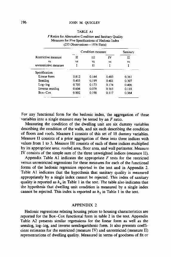
As noted in the text, the measure of sanitary quality consists of eight dummy variables indicating the presence of particular plumbing and sani- tary facilities. Prior to the analysis, these eight dummy variables (measure I) were aggregated to a single index (measure II) with values range from 1 to 4.

JOHN M. QUIGLEY

TABLE Al F Ratios for Alternative Condition and Sanitary Quality

Measures for Five Specifications of Hedonic Index (253 Observations- 1976 Data)

Restrictive measure vs

unrestrictive measure

Condition measure

II III IV vs vs vs I II I

Specification Linear form Semilog Log-log Inverse semilog Box-Cox

0.812 0.144 0.483 0.361 0.403 0.199 0.48 I 0.307 0.703 0.173 0.174 0.406 0.604 0.078 0.165 0.118 0.802 0.198 0.117 0.364

Sanitary

II vs I

For any functional form for the hedonic index, the aggregation of these variables into a single measure may be tested by an F ratio.

Measuring the condition of the dwelling unit are six dummy variables describing the condition of the walls, and six each describing the condition of floors and roofs. Measure I consists of this set of 18 dummy variables. Measure II consists of a prior aggregation of these into three indices with values from 1 to 3. Measure III consists of each of these indices multiplied by its appropriate area: roofed area, floor area, and wall perimeter. Measure IV consists of the simple sum of the three unweighted indices (measure II).

Appendix Table Al indicates the appropriate F tests for the restricted versus unrestricted regressions for these measures for each of the functional forms of the hedonic regression reported in the text and in Appendix 2. Table Al indicates that the hypothesis that sanitary quality is measured appropriately by a single index cannot be rejected. This index of sanitary quality is reported as h, in Table 1 in the text. The table also indicates that the hypothesis that dwelling unit condition is measured by a single index cannot be rejected. This index is reported as h, in Table 1 in the text.

APPENDIX 2

Hedonic regressions relating housing prices to housing characteristics are reported for the Box-Cox functional form in table 2 in the text. Appendix Table A2 presents similar regressions for the linear form as well as the semilog, log-log, and inverse semilogarithmic form. It also presents coeffi- cient estimates for the restricted (measure IV) and unrestricted (measure II) representations of dwelling quality. Measured in terms of goodness of fit or

NONLINEAR BUDGET CONSTRAINTS AND CONSUMER DEMAND 197

significance levels of coefficients, there is little basis to choose among specifications. The alternative forms explain between 33% and 38% of the variation in rent, with a slightly higher explained variation for the semilog form. In contrast, the Box-Cox specification reported in Table 2 in the text accounts for 49% of the variation in monthly rents, and the t ratios of coefficients are slightly larger.

APPENDIX 3

Two of the attributes of housing, piped water and electricity, are inher- ently discrete and their parameters cannot be estimated from the first-order conditions (IQ. (20) in the text). Thus the 11 parameters of the GCES utility function reported in Table 3 in the text are incomplete; they neglect, for example, the possibility that households trade off more space for piped water.

TABLE A2 Alternative Functional Forms and Constraints for Hedonic Regressions (253 Observations- 1976 Data)

Linear form Semilog Log-Log Inverse semilog

Coefficients 1 2 3 4 5 6 7 8

Number of rooms 10.770 (8.38)

Living area 0.661 (meters’ X 10) (2.01)

Lot size 0.528 (meters* X 10) (0.70)

Electricity 2.904 (I = available) (1.34)

Piped water 2.759 (1 = available) (1.14)

Sanitary quality 3.465 (3.52)

Floor condition 1.365 (0.52)

Wall condition 0.753 (0.39)

Roof condition 3.875 (0.75)

Aggregate condition

Intercept -17.270 - (1.43)

R* 0.363 R* in original space 0.363 SEE/mean 0.438 F test of quality

coefficient equality

10.750 (8.41) 0.653

(2.W 0.477

(0.64) 2.823

(1.34) 2.669

(1.12) 3.501

(3.59)

1.233 (0.89) 12.550 (1.51) 0.363 0.363 0.436

0.144 0.199 0.173 0.078

0.374 (7.72) 0.028

(2.22) 0.034

(1.20) 0.159

(1.95) 0.184

(2.02) 0.093

(2.51) 0.077

(0.78) 0.075

(1.W 0.205

(1.05)

1.224 (2.68) 0.358 0.384 0.124

0.373 (7.71) 0.028

(2.19) 0.033

(1.15) 0.153

(1.91) 0.178

(1.97)

(2.58)

0.088 (1.68)

1.419 (4.52) 0.357 0.384 0.124

0.573 (7.61) 0.027

(2.16) 0.412

(1.59) 0.154

(1.87) 0.173

(1.84) 0.178

(2.50) 0.067

(0.47) 0.142

(1.W 0.258

(0.75)

2.070

(7.44) 0.345 0.353 0.125

0.574 (7.67) 0.027

(2.19) 0.405

(1.57) 0.147

(1.82) 0.167

(1.80) 0.181

(2.55)

0.423 (1.48) 1.646

(3.23) 0.345 0.353 0.125

16.030 (7.92) 0.068

(2.02) 0.760

(1.09) 2.857

(1.29) 2.492

(0.98) 6.149

(3.20) 0.898

(0.23) 1.925

(0.53) 4.586

(0.50)

3.497 (0.47) 0.333 0.333 0.448

16.041 (7.98) 0.068

(2.03) 0.748

(1.08) 2.742

(1.27) 2.373

(0.95) 6.209

(3.26)

5.917 (0.77)

-1.788 (0.13) 0.333 0.333 0.446

198 JOHN M. QUIGLEY

In the sample of 249 Santa Ana households, 92% had piped water in their dwelling units and 89% had electricity in 1976. How do households sub- stitute between these two attributes and the other characteristics of the bundle of housing and other goods?

It should be clear that if households are informed customers, then, in equilibrium, all households of the same income and family size will achieve the same level of satisfaction regardless of their consumption choices. Thus, if we consider households of the same income and family size, the computed values of the utility function must be identical. Therefore, within any group of homogeneous households, differences in the value of the utility index computed from the coefficients in Table 3 must be attributable to variations in these amenities.

If we partition “identical” households (i.e., those of the same income and family size) we can compute the utility index for four groups of households: Those with both water and electricity (U,,); those with water (U,O); those with electricity (&,); and those with neither (U,). For each group of identical households, it must be true that:

The solution of two of the three equations will provide the values of a6 and (r7 for each class of identical consumers. Note that this does not compare utilities across households of differing incomes and family sizes. Households of the same income and family size are assumed to be identical. Competition insures they achieve identical utility levels. Thus

U = f (income, family size),

Consider those 207 households choosing both piped water and electricity. A regression of the computed value of utility U,, from the GCES function reported in the text upon income and family size yields

U,, = U, + a6 + (Ye = 4.550 + 5.484 (income)- 0.514 (family size), (3.90) (127.40) (2.36)

R= = 0.988, (A-1 >

where t ratios are in parentheses. For each of the 249 households in the entire sample, the coefficients of

(A-l) provide a value of c,, or (0, + a6 + ar,), the utility achieved by households if they had chosen both piped water and electricity. Since utilities must be equalized regardless of whether these attributes are chosen, the utility level estimated from (A-l) can only differ from the utility level

NONLINEAR BUDGET CONSTRAINTS AND CONSUMER DEMAND 199

computed from the GCES function (I?) due to the presence of water or electricity, i.e.,

fi + ag (piped water) + a, (electricity) = o,, . (A-2)

A regression of the difference, between the utility level computed from the GCES expression and the utility level computed from (A-l) if house- holds had chosen water and electricity, upon these dummy variables yields, for the sample of 249 observations:

fi - fi,, = 5.249 - 2.349 (piped water) -2.864 (electricity), (3.107) (1.54) (2.67)

R= = 0.034,

where t ratios are in parentheses. a6 is estimated to be 2.349; a7 is estimated to be 2.864.

Application of the same methodology to the CES utility function yields coefficients of 2.046 and 2.617 for piped water and electricity.

APPENDIX 4

As noted in the text, the benefits to program participants can be aggre- gated to indicate the total benefits of a public program to renters if the program is “small” or if the local economy is “open.” Clearly if the program were large or if the economy were closed-if a sizable fraction of households within a single market were participants or if there were barriers to mm&ration-then some benefits would accrue to nonparticipants in the form of lower prices in the private housing market.

The existence of cross sectional observations on dwelling units and their prices before and after the subsidy program was initiated permits this issue to be investigated.

Table A4 summarizes the observed differences in the structure of housing prices in the market between 1976 (before any households had moved into subsidized units) and 1979 (approximately two years after participating households had moved into their subsidized units). The table reports the explained variance in monthly rent for regressions based on three samples: the pooled sample of dwelling units in the private economy in 1976 and 1979; and separately for the 1976 and 1979 samples.

These regressions relate monthly rent to the seven independent variables for five different functional forms. The table also reports the t ratio for a dummy variable in the pooled regression for 1979 observations, and the F ratio testing the hypothesis that the structure of housing prices was different between the two years. Both hypotheses are rejected by a wide margin,

JOHN M. QUIGLEY

TABLE A4 Covariance Tests for Homogeneity of Hedonic

Coefficients for 1976 and 1979 Samples of Dwelling Units

Functional form

Linear R=

t F

Box-Cox R2

t F

Semilog R2

t F

Log-Log R2

t F

Inverse semilog R2

t F

Pooled sample

0.387 0.249 0.873

0.373 0.187 0.882

0.385 0.178 0.814

0.377 0.683 0.900

0.357 0.714 I.419

1976 1979 sample sample

0.363 0.399

0.343 0.343

0.357 0.365

0.345 0.370

0.333 0.394

indicating that the structure of housing prices remained the same. Since the subsidy program had no impact on housing prices in the market, then all benefits accrue to participants.

REFERENCES I. G. E. P. Box and D. R. Cox, An analysis of transformations, J. Roy. Statist. Sot. Ser. B, 26

(19w. 2. J. N. Brown and H. S. Rosen, On the estimation of structural hedonic price models,

Econometricrr (May 1982). 3. M. Edel, Land values and the costs of urban congestion, Social Sci. Inform. (1971). 4. A. M. Freeman, III, The hedonic approach to measuring demand for neighborhood

characteristics, in “The Economics of Neighborhood,” (David Segal, Ed.), Academic Press, New York (1979).

5. A. Goodman, Hedonic prices, price indices, and housing markets, J. Urban Econ., (October 1978).

6. 2. Griliches, Hedonic price indexes for automobiles: An econometric analysis of quality change, in “Price Statistics of the Federal Government,” U.S. Gov’t. Priming Office, Washington, D.C. (1961).

7. D. Harrison and D. Rubinfeld, Hedonic house prices and the demand for clean air, J. Environ. Econ. Munug., 5 (1978).

NONLINEAR BUDGET CONSTRAINTS AND CONSUMER DEMAND 201

8. J. F. Kain and J. M. Quigley, “Housing Markets and Racial Discrimination,” Nat. Bur. Econ. Res., New York, London (1975).

9. M. P. Murray, The distribution of tenant benefits in public housing, Econometn‘ca (July 1975).

10. M. P. Murray, Methodologies for estimating housing subsidy benefits, Public Finance Quart. (April 1978).

Il. R. J. Olsen, The method of Box and Cox-A pitfall, J. Amer. Statist. Assoc., in press. 12. Y. Oron, D. Pines, and E. She&in&i, The effect of nuisances associated with urban traffic

on suburbanization and land values, J. Urban Econ. (October 1974). 13. A. M. Polinsky and D. L. Rubinfeld, Property values and the benefits of environmental

improvements: Theory and measurement, in “Public Economics and the Quality of Life” (Lowdon Wingo and Alan Evans, Eds.), Johns Hopkins Univ. Press, Baltimore (1977).

14. J. M. Quigley, The distributional consequences of stylized housing programs: Theory and empirical analysis, August 1980, mimeo.

15. R. G. Ridker and J. A. Henning, The determinants of residential property values with special reference to air pollution, Reu. Econ. Srarisr. (May 1967).

16. S. Rosen, Hedonic prices and implicit markets: Product differentiation in pure competi- tion, J. PO/. Econ. (Jan./Feb. 1974).

17. J. E. Triplett, Consumer demand and characteristics of consumption goods, in “Household Production and Consumption” (Nestor E. Terleckyj, Ed.), Nat. Bur. Econ. Res., New York, London (1975).

18. A. A. Walters, “Noise and Prices,” Oxford Univ. Press (Clarendon), London (1975). 19. A. D. Witte, H. J. Sumka, and H. Erekson, An estimate of a structural hedonic price model

of the housing market: An application of Rosen’s theory of implicit markets, Econometrica (September 1979).

20. The World Bank, “Housing,” Sector Policy Paper, May 1975.