
Nonintersecting Brownian motions on the unit...
78
The Annals of Probability 2016, Vol. 44, No. 2, 1134–1211 DOI: 10.1214/14-AOP998 © Institute of Mathematical Statistics, 2016 NONINTERSECTING BROWNIAN MOTIONS ON THE UNIT CIRCLE BY KARL LIECHTY AND DONG WANG 1 DePaul University and National University of Singapore We consider an ensemble of n nonintersecting Brownian particles on the unit circle with diffusion parameter n −1/2 , which are conditioned to begin at the same point and to return to that point after time T , but otherwise not to intersect. There is a critical value of T which separates the subcritical case, in which it is vanishingly unlikely that the particles wrap around the circle, and the supercritical case, in which particles may wrap around the circle. In this paper, we show that in the subcritical and critical cases the probability that the total winding number is zero is almost surely 1 as n →∞, and in the supercritical case that the distribution of the total winding number converges to the discrete normal distribution. We also give a streamlined approach to identifying the Pearcey and tacnode processes in scaling limits. The formula of the tacnode correlation kernel is new and involves a solution to a Lax system for the Painlevé II equation of size 2 × 2. The proofs are based on the determinantal structure of the ensemble, asymptotic results for the related system of discrete Gaussian orthogonal polynomials, and a formulation of the correlation kernel in terms of a double contour integral. 1. Introduction. The probability models of nonintersecting Brownian mo- tions have been studied extensively in last decade; see Tracy and Widom (2004, 2006), Adler and van Moerbeke (2005), Adler, Orantin and van Moerbeke (2010), Delvaux, Kuijlaars and Zhang (2011), Johansson (2013), Ferrari and Vet˝ o (2012), Katori and Tanemura (2007) and Schehr et al. (2008), for example. These models are closely related to random matrix theory and (multiple) orthogonal polynomials; see Bleher and Kuijlaars (2004, 2007), Aptekarev, Bleher and Kuijlaars (2005) and Kuijlaars (2010), for example. One interesting feature is that as the number of par- ticles n →∞, under proper scaling the nonintersecting Brownian motions models converge to universal processes, like the sine, Airy, Pearcey and tacnode processes. These processes are called universal since they appear in many other probability problems; see Okounkov and Reshetikhin (2003, 2007), Johansson (2005), Baik and Suidan (2007), Adler, van Moerbeke and Wang (2013), Adler, Ferrari and van Moerbeke (2013) and Adler, Johansson and van Moerbeke (2014), for example. Received July 2014; revised December 2014. 1 Supported in part by the startup Grant R-146-000-164-133. MSC2010 subject classifications. Primary 60J65; secondary 35Q15, 42C05. Key words and phrases. Nonintersecting Brownian motions, determinantal process, discrete or- thogonal polynomial, tacnode process, Pearcey process, Riemann–Hilbert problem, double contour integral formula. 1134
Transcript of Nonintersecting Brownian motions on the unit...

The Annals of Probability2016, Vol. 44, No. 2, 1134–1211DOI: 10.1214/14-AOP998© Institute of Mathematical Statistics, 2016
NONINTERSECTING BROWNIAN MOTIONSON THE UNIT CIRCLE
BY KARL LIECHTY AND DONG WANG1
DePaul University and National University of Singapore
We consider an ensemble of n nonintersecting Brownian particles on theunit circle with diffusion parameter n−1/2, which are conditioned to begin atthe same point and to return to that point after time T , but otherwise not tointersect. There is a critical value of T which separates the subcritical case,in which it is vanishingly unlikely that the particles wrap around the circle,and the supercritical case, in which particles may wrap around the circle. Inthis paper, we show that in the subcritical and critical cases the probabilitythat the total winding number is zero is almost surely 1 as n→ ∞, and in thesupercritical case that the distribution of the total winding number convergesto the discrete normal distribution. We also give a streamlined approach toidentifying the Pearcey and tacnode processes in scaling limits. The formulaof the tacnode correlation kernel is new and involves a solution to a Laxsystem for the Painlevé II equation of size 2 × 2. The proofs are based onthe determinantal structure of the ensemble, asymptotic results for the relatedsystem of discrete Gaussian orthogonal polynomials, and a formulation of thecorrelation kernel in terms of a double contour integral.
1. Introduction. The probability models of nonintersecting Brownian mo-tions have been studied extensively in last decade; see Tracy and Widom (2004,2006), Adler and van Moerbeke (2005), Adler, Orantin and van Moerbeke (2010),Delvaux, Kuijlaars and Zhang (2011), Johansson (2013), Ferrari and Veto (2012),Katori and Tanemura (2007) and Schehr et al. (2008), for example. These modelsare closely related to random matrix theory and (multiple) orthogonal polynomials;see Bleher and Kuijlaars (2004, 2007), Aptekarev, Bleher and Kuijlaars (2005) andKuijlaars (2010), for example. One interesting feature is that as the number of par-ticles n→ ∞, under proper scaling the nonintersecting Brownian motions modelsconverge to universal processes, like the sine, Airy, Pearcey and tacnode processes.These processes are called universal since they appear in many other probabilityproblems; see Okounkov and Reshetikhin (2003, 2007), Johansson (2005), Baikand Suidan (2007), Adler, van Moerbeke and Wang (2013), Adler, Ferrari and vanMoerbeke (2013) and Adler, Johansson and van Moerbeke (2014), for example.
Received July 2014; revised December 2014.1Supported in part by the startup Grant R-146-000-164-133.MSC2010 subject classifications. Primary 60J65; secondary 35Q15, 42C05.Key words and phrases. Nonintersecting Brownian motions, determinantal process, discrete or-
thogonal polynomial, tacnode process, Pearcey process, Riemann–Hilbert problem, double contourintegral formula.
1134

NONINTERSECTING BROWNIAN MOTIONS 1135
Usually the models of nonintersecting Brownian motions turn out to be the mostconvenient ones to use for study of these universal processes. In particular, theAiry process appears ubiquitously in the Kardar–Parisi–Zhang (KPZ) universal-ity class [Corwin (2012)], an important class of interacting particle systems andrandom growth models. The analysis of nonintersecting Brownian motions greatlyimproves the understanding of the Airy process and the KPZ universality class;see Corwin and Hammond (2014). Here, we remark that if we consider the nonin-tersecting Brownian motions on the real line, in the simplest models the Pearceyprocess does not occur, and the tacnode process only occurs in models with so-phisticated parameters. Thus, the analysis of these universal processes becomesincreasingly more difficult.
Due to technical difficulties, most studies of the limiting local properties ofthe nonintersecting Brownian motions concern models defined on the real line.A model of nonintersecting Brownian motions on a circle was considered byDyson as a dynamical generalization of random matrix models [Dyson (1962)],and physicists and probabilists have been interested in the nonintersecting Brow-nian motions on a circle and their discrete counterparts for various reasons; seeForrester (1990), Hobson and Werner (1996) and Cardy (2003), for example. Thesimplest model of nonintersecting Brownian motions on a circle such that the par-ticles start and end at the same common point is shown to be related to Yang–Millstheory on the sphere [Forrester, Majumdar and Schehr (2011), Schehr et al. (2013)]and the partition function (a.k.a. reunion probability) shows an interesting phasetransition phenomenon closely related to the Tracy–Widom distributions in ran-dom matrix theory.
In this paper, we show that the Pearcey and (symmetric) tacnode processes men-tioned above occur as the limits of the simplest model of nonintersecting Brownianmotions on a circle, and give a streamlined method to analyze them. We also con-sider the total winding number of the particles, a quantity that has no counterpartin the models defined on the real line, and show that its limiting distribution inthe nontrivial case is the discrete normal distribution [Szabłowski (2001)], a natu-ral through perhaps not well-known discretization of the normal distribution. Wealso show that in the supercritical case, the Pearcey process occurs if the model isconditioned to have fixed total winding number. Although the sine and Airy pro-cesses also naturally occur, we omit the discussion on them to shorten the paper.A detailed discussion can be found in the preprint [Liechty and Wang (2013)].
Technically, the study of nonintersecting Brownian motions has been carriedout in two distinct ways: by double contour integral formula, and by the Riemann–Hilbert problem. In the present work, we introduce a mixed approach, using botha double integral formula and the interpolation problem for discrete Gaussian or-thogonal polynomials [Liechty (2012)], which are discrete orthogonal polynomialsanalogous to Hermite polynomials. In this paper, we analyze the dependence of thediscrete Gaussian orthogonal polynomials on the translation of the lattice, whichencodes the information of the winding number of the Brownian paths.

1136 K. LIECHTY AND D. WANG
1.1. Statement of main results. Let T = {eiθ ∈ C} be the unit circle. Supposex1, x2, . . . , xn are n particles in independent Brownian motions on the unit circlewith continuous paths and diffusion parameter n−1/2, that is,
xk(t)= eiBk(t)/√n, i = 1,2, . . . , n,(1)
whereBk(t) are independent Brownian motions with diffusion parameter 1 startingfrom arbitrary places. The nonintersecting Brownian motions on the circle with nparticles, henceforth denoted as NIBM in this paper, is defined by the particlesx1, . . . , xn conditioned to have nonintersecting paths, that is, x1(t), . . . , xn(t) aredistinct for any t between the starting time and the ending time. In this paper, weconcentrate on the simplest model of NIBM, such that the n particles start from thecommon point ei·0 at the starting time t = 0, and end at the same common pointei·0 at the ending time t = T . We denote this model as NIBM0→T .
Throughout this paper, we represent a point in T by an angular variable θ ∈ R
with θ = θ + 2πk (k ∈ Z) if there is no possibility of confusion, and use θ ∈[−π,π) as the principal value of the angle. Let P(a;b; t) be the transition prob-ability density of one particle in Brownian motion on T with diffusion parametern−1/2, starting from point a ∈ T and ending at point b ∈ T after time t > 0, whichis
P(a;b; t)=√n
2πt
∑k∈Ze−n(b−a+2πk)2/(2t).(2)
Now consider the transition probability density of NIBM. Let An = {a1, . . . , an}and Bn = {b1, . . . , bn} be two sets of n distinct points in T such that −π ≤ a1 <
a2 < · · ·< an < π and −π ≤ b1 < b2 < · · ·< bn < π , and denote by P(An;Bn; t)the transition probability density of NIBM with the particles starting at the pointsAn and ending at the points Bn after time t . Note that we do not require that theparticle which started at point ak ends at point bk , but only that it ends at point bjfor some j = 1, . . . , n. For τ ∈ R, introduce the notation
P(a;b; t; τ) :=√n
2πt
∑k∈Ze−n(b−a+2πk)2/(2t)e2kπτ i,(3)
which reduces to (2) when τ = 0. Introduce also the notation
ε(n)={0, if n is odd,
12 , if n is even.
(4)
A determinantal formula for P(An;Bn; t) is then given in the following proposi-tion.
PROPOSITION 1.1. The transition probability density function P(An;Bn; t)is given by the determinant of size n× n,
P(An;Bn; t)= det(P(ai;bj ; t; ε(n)))ni,j=1.(5)
NONINTERSECTING BROWNIAN MOTIONS 1137
This proposition follows immediately from the Karlin–McGregor formula in thecase that n is odd. If n is even then more care must be taken to derive the formula,and in the limited knowledge of the current authors it has not appeared before inthe literature. The proof is presented in Section 2.1.
Now we consider the model NIBM0→T . At a given time t ∈ [0, T ], the jointprobability density function for the n particles in NIBM0→T at distinct points−π ≤ θ1 < θ2 < · · ·< θn < π is given by
lima1,...,an→0b1,...,bn→0
P(An;�n; t)P (�n;Bn;T − t)P (An;Bn;T ) ,(6)
where An = {a1, . . . , an}, Bn = {b1, . . . , bn}, and �n = {θ1, . . . , θn} describe thelocations of the n particles at time 0, T and t , respectively. It is not difficult to seethat such a limit exists, and so that our model is well defined (see Section 2.2).
The model NIBM0→T is a determinantal process, meaning that the correlationfunctions of the particles may be described by a determinantal formula [Soshnikov(2000)]. To define the determinantal structure, fixm times 0< t1 < t2 < · · ·< tm <T , and to each time ti , fix ki points on T, −π ≤ θ(i)1 < θ
(i)2 < · · ·< θ(i)ki < π . The
multi-time correlation function is then defined as
R(n)0→T
(θ(1)1 , . . . , θ
(1)k1
; . . . ; θ(m)1 , . . . , θ(m)km
; t1, . . . , tm):= lim
�x→0
1
(�x)k1+···+km P(there is a particle in
[θ(i)j , θ
(i)j +�x)(7)
for j = 1, . . . , ki at time ti).
Then there exists some kernel function Kti,tj (x, y) such that
R(n)0→T
(θ(1)1 , . . . , θ
(1)k1
; . . . ; θ(m)1 , . . . , θ(m)km
; t1, . . . , tm)(8)
= det(Kti,tj
(θ(i)li, θ(j)
l′j
))i,j=1,...,m,li=1,...,ki ,l′j=1,...,kj
;see Section 2.3.
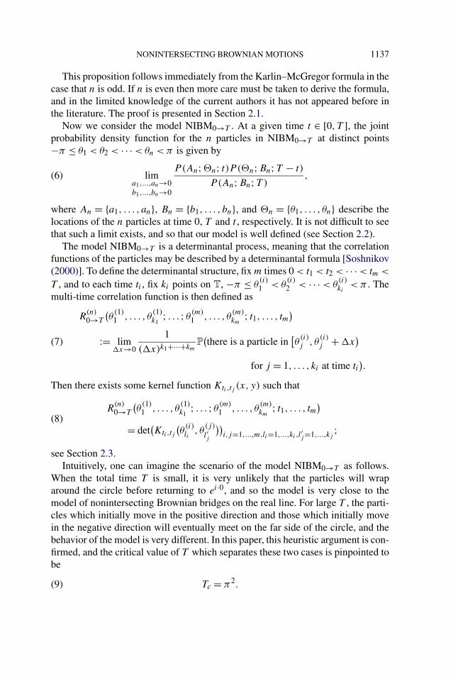
Intuitively, one can imagine the scenario of the model NIBM0→T as follows.When the total time T is small, it is very unlikely that the particles will wraparound the circle before returning to ei·0, and so the model is very close to themodel of nonintersecting Brownian bridges on the real line. For large T , the parti-cles which initially move in the positive direction and those which initially movein the negative direction will eventually meet on the far side of the circle, and thebehavior of the model is very different. In this paper, this heuristic argument is con-firmed, and the critical value of T which separates these two cases is pinpointed tobe
Tc = π2.(9)
1138 K. LIECHTY AND D. WANG
FIG. 1. Typical configurations of nonintersecting paths in the subcritical (left), critical (middle)and supercritical (right) cases. Time is on the vertical axis, and the angular variable θ on the hor-izontal axis. At the initial time t = 0 and the terminal time t = T , the particles are at θ = 0, whichis at both the left and right ends of the figures. The far side of the circle, θ = ±π , is marked by alight vertical line through the center of the figures. The particles tend to stay within the thick curvedlines. In the supercritical case, the critical time tc is marked, when the “leftmost” and “rightmost”particles meet on the far side of the circle.
Accordingly, we divide the NIBM0→T model into the subcritical, critical and su-percritical cases, for T < π2, T = π2, and T > π2, respectively, as shown in Fig-ure 1.
In the subcritical case T < Tc, the model is described asymptotically by ele-mentary functions. In the critical case T = Tc and the supercritical case T > Tc,the model is described asymptotically by special functions: functions related tothe Painlevé II equation for T = Tc, and elliptic integrals for T > Tc. Let us definethose functions.
Critical case: The Painlevé II equation, and the related Lax pair. In the criticalcase, we consider the model NIBM0→T in the scaling limit
T = π2(1 − 2−2/3σn−2/3),(10)
where σ ∈R is a parameter. In this case, the results of this paper involve a particu-lar solution to the Painlevé II equation, and a solution to a related Lax system. Letus review these objects. The Hastings–McLeod solution [Hastings and McLeod(1980)] to the homogeneous Painlevé II equation (PII) is the solution to the differ-ential equation
q ′′(s)= sq(s)+ 2q(s)3,(11)
which satisfies
q(s)= Ai(s)(1 + o(1)) as s→ +∞,(12)
NONINTERSECTING BROWNIAN MOTIONS 1139
where Ai(s) is the Airy function. Let q(s) be this particular solution to PII, andconsider the 2 × 2 matrix-valued solutions to the differential equation
d
dζ�(ζ ; s)=
(−4iζ 2 − i(s + 2q(s)2)
4ζq(s)+ 2iq ′(s)4ζq(s)− 2iq ′(s) 4iζ 2 + i(s + 2q(s)2
))�(ζ ; s).(13)
This 2 × 2 system was originally studied by Flaschka and Newell (1980). Thedifferential equation (13), together with another one given in (340), form a Laxpair for the PII equation, that is, the compatibility of the two differential equationsimplies that q(s) solves PII. We will consider the particular solution to (13) whichsatisfies
�(ζ ; s)ei((4/3)ζ 3+sζ )σ3 = I +O(ζ−1), ζ → ±∞.(14)
The asymptotics (14) extend into the sectors −π/3 < arg ζ < π/3, and 2π/3 <arg ζ < 4π/3. Here, we note that the uniqueness of the boundary value prob-lem (13) and (14) implies
i,j (−ζ )=3−i,3−j (ζ ), i, j = 1,2.(15)
Supercritical case: Elliptic integrals. In the supercritical case where T > Tc =π2, we define a tc < T/2. To simplify the notation, we parametrize T > π2 byk ∈ (0,1). For each k, we have the elliptic integrals
K := K(k)=∫ 1
0
ds√(1 − s2)(1 − k2s2)
,
(16)
E := E(k)=∫ 1
0
√1 − k2s2
√1 − s2
ds.
We further define
k := 2√k
1 + k ,(17)
and denote
K := K(k)=∫ 1
0
ds√(1 − s2)(1 − k2s2)
,
(18)
E := E(k)=∫ 1
0
√1 − k2s2√
1 − s2ds.
T is then parametrized as
T = 4KE = 4∫ 1
0
ds√(1 − s2)(1 − k2s2)
∫ 1
0
√1 − k2s2√
1 − s2ds,(19)

1140 K. LIECHTY AND D. WANG
where the well-definedness of the parametrization is given in Lemma 3.2, and tc
is expressed as
tc = 4
k2E(E − (
1 − k2)K) = 4∫ 1
0
√1 − k2s2√
1 − s2ds
∫ 1
0
√1 − s2√
1 − k2s2ds.(20)
The fundamental group of T has a canonical identification with Z, and so forany closed path on T we can define the winding number of the path as the inte-ger representative of its homotopy class. For a set of n particles with continuouspaths on T that come back the initial position after some time, we can define theirtotal winding number as the sum of the winding numbers of the paths of the parti-cles. The following theorem concerns the total winding number of the particles inNIBM0→T . Let q be defined in terms of the complete elliptic integral of the firstkind as
q := exp(−πK(
√1 − k2)
2K(k)
)= exp
(−πK(
√1 − k2)
K(k)
),(21)
where k and k are related to T via (16)–(19).
REMARK 1.1. Note that we use the notation q in two different meanings.In the context of the critical asymptotics, q is the Hastings–McLeod solution toPII and is always written with its argument q(σ ). In the context of the supercriticalasymptotics, q is written with no argument and represents the elliptic nome definedin (21). These are both standard notation, and it should be clear throughout thepaper to which object q refers.
THEOREM 1.2. In the NIBM0→T , as the number of particles n→ ∞:
(a) In the subcritical case T < Tc = π2, the winding number is zero with aprobability that is exponentially close to 1. That is,
P(Total winding number equals 0)= 1 −O(e−cn
),(22)
where the constant c > 0 may depend on T .(b) In the critical scaling (10), for any fixed σ ,
P(Total winding number equals 0)= 1 − q(σ )
21/3n1/3 + q(σ )2
22/3n2/3 +O(n−1),
P(Total winding number equals 1)= P(Total winding number equals (−1)
)(23)
= q(σ )
24/3n1/3 − q(σ )2
25/3n2/3 +O(n−1),
P(|Total winding number|> 1
) = O(n−1).

NONINTERSECTING BROWNIAN MOTIONS 1141
FIG. 2. The shape of contours �P and �P . The upper part of �P consists of the ray from 2 + 2ito eπi/4 · ∞, the line segment from to 2 + 2i to −2 + 2i, and the ray from −2 + 2i to e3πi/4 · ∞.The lower part of �P is the reflection of the upper part about the real axis. �P is the horizontal line{z= x + i|x ∈R}. Their orientations are shown in the figure.
(c) For T > Tc and for any ω ∈ Z,
P(Total winding number equals ω)= qω2
√π
2K+O
(n−1).(24)
The limiting distribution of the total winding number in the supercritical caseis the discrete normal distribution defined in Kemp (1997), and the formula in theright-hand side of (24) appears in Szabłowski (2001). See also Johnson, Kemp andKotz (2005), Section 10.8.3.
The Pearcey process is defined by the extended Pearcey kernel [Tracy andWidom (2006), Section 3],
KPearceys,t (ξ, η)= KPearcey
s,t (ξ, η)− φs,t (ξ, η),(25)
where
φs,t (ξ, η)=⎧⎨⎩
0, if s ≥ t ,1√
2π(t − s)e−(ξ−η)2/(2(t−s)), if s < t ,(26)
and
KPearceys,t (ξ, η)= i
4π2
∮�P
dz
∮�P
dwez
4/4+sz2/2+iξz
ew4/4+tw2/2+iηw
1
z−w,(27)
where �P and �P are infinite, disjoint contours such that the upper part of �P isfrom eπi/4 · ∞ to e3πi/4 · ∞, the lower part of �P is from e5πi/4 · ∞ to e7πi/4 ·∞, and �P is the leftward horizontal line. See Figure 2 for the exact description.Our definition of the Pearcey kernel is the same as that in Adler, Orantin and vanMoerbeke (2010), Formula 1.2, up to a change of variables.
1142 K. LIECHTY AND D. WANG
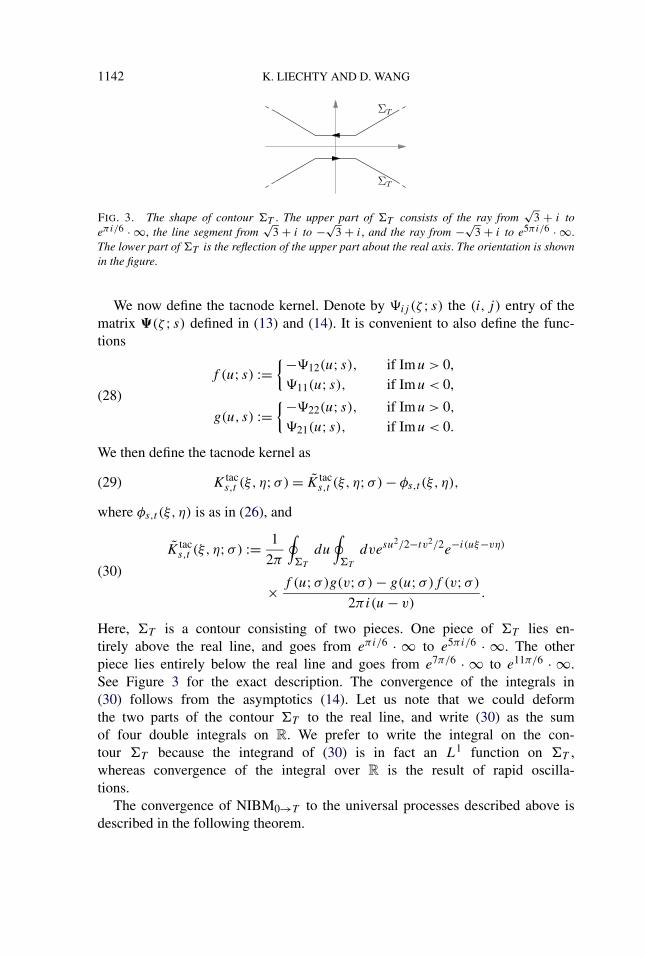
FIG. 3. The shape of contour �T . The upper part of �T consists of the ray from√
3 + i toeπi/6 · ∞, the line segment from
√3 + i to −√
3 + i, and the ray from −√3 + i to e5πi/6 · ∞.
The lower part of �T is the reflection of the upper part about the real axis. The orientation is shownin the figure.
We now define the tacnode kernel. Denote by ij (ζ ; s) the (i, j) entry of thematrix �(ζ ; s) defined in (13) and (14). It is convenient to also define the func-tions
f (u; s) :={−12(u; s), if Imu > 0,11(u; s), if Imu < 0,
(28)
g(u, s) :={−22(u; s), if Imu > 0,21(u; s), if Imu < 0.
We then define the tacnode kernel as
K tacs,t (ξ, η;σ)= K tac
s,t (ξ, η;σ)− φs,t (ξ, η),(29)
where φs,t (ξ, η) is as in (26), and
K tacs,t (ξ, η;σ) :=
1
2π
∮�T
du
∮�T
dvesu2/2−tv2/2e−i(uξ−vη)
(30)
× f (u;σ)g(v;σ)− g(u;σ)f (v;σ)2πi(u− v) .
Here, �T is a contour consisting of two pieces. One piece of �T lies en-tirely above the real line, and goes from eπi/6 · ∞ to e5πi/6 · ∞. The otherpiece lies entirely below the real line and goes from e7π/6 · ∞ to e11π/6 · ∞.See Figure 3 for the exact description. The convergence of the integrals in(30) follows from the asymptotics (14). Let us note that we could deformthe two parts of the contour �T to the real line, and write (30) as the sumof four double integrals on R. We prefer to write the integral on the con-tour �T because the integrand of (30) is in fact an L1 function on �T ,whereas convergence of the integral over R is the result of rapid oscilla-tions.
The convergence of NIBM0→T to the universal processes described above isdescribed in the following theorem.
NONINTERSECTING BROWNIAN MOTIONS 1143
THEOREM 1.3. In the NIBM0→T :
(a) Assume T > Tc. There exists d > 0 defined in (235) such that when we scaleti and tj close to tc, and x and y close to −π as
ti = tc + d2
n1/2 τi, tj = tc + d2
n1/2 τj ,
(31)
x = −π − d
n3/4 ξ, y = −π − d
n3/4η,
the correlation kernel Kti,tj (x, y) has the limit
limn→∞Kti,tj (x, y)
∣∣∣∣dydη∣∣∣∣ =KPearcey
−τj ,−τi (η, ξ).(32)
(b) Let T be scaled close to Tc = π2 as in (10) with σ fixed, and let
d = 2−5/3π.(33)
When we scale ti and tj close to T/2, and x and y close to −π as
ti = T
2+ d2
n1/3 τi, tj = T
2+ d2
n1/3 τj ,
(34)
x = −π − d
n2/3 ξ, y = −π − d
n2/3η,
the correlation kernel Kti,tj (x, y) has the limit
limn→∞Kti,tj (x, y)
∣∣∣∣dydη∣∣∣∣ =K tac
τi ,τj(ξ, η;σ)=K tac−τj ,−τi (η, ξ ;σ).(35)
REMARK 1.2. The identity K tacτi ,τj
(ξ, η;σ)=K tac−τj ,−τi (η, ξ ;σ) in (35) is due
to the symmetry of the kernel K tacs,t (ξ, η), which can be checked by (15).
In the supercritical case, we have finer result for the NIBM0→T conditionedto have fixed total winding number. Analogous to (7), we define the multi-timecorrelation function for the NIBM0→T with total winding number ω as(
R(n)0→T
)ω
(a(1)1 , . . . , a
(1)k1
; . . . ;a(m)1 , . . . , a(m)km
; t1, . . . , tm)(36)
:= lim�x→0
1
(�x)k1+···+km P
⎛⎜⎝ there is a particle in
[a(i)j , a
(i)j +�x)
for j = 1, . . . , ki at time ti ,and the total winding number is ω
⎞⎟⎠ .
If we consider the conditional NIBM0→T such that the total winding number isfixed to be ω, then the multi-time correlation function of the conditional process
1144 K. LIECHTY AND D. WANG
should be(R(n)0→T
)∼ω
(a(1)1 , . . . , a
(1)k1
; . . . ;a(m)1 , . . . , a(m)km
; t1, . . . , tm)(37)
:= (R(n)0→T )ω(a
(1)1 , . . . , a
(1)k1
; . . . ;a(m)1 , . . . , a(m)km
; t1, . . . , tm)P(Total winding number equals ω)
.
Note that if the total winding number is fixed, then the conditional NIBM0→T isno longer a determinantal process. (The reason is as follows: In a determinantalprocess over time [0, T ], the movement of particles between two times t1 < t2 ∈(0, T ) only depends on the positions of the particles at times t1 and t2, but notthe trajectories on (0, t1) or (t2, T ). The conditional NIBM0→T with fixed totalwinding number does not have this property.) Nevertheless, we have results for thelimiting k-correlation functions of the process. The following theorem shows thatwith the condition of fixed total winding number, the conditional NIBM0→T hasthe same local limiting properties as the NIBM0→T with free winding number.
THEOREM 1.4. Assume T > Tc = π2. Let ω be a fixed integer, t1, . . . , tm ∈(0, T ) be times, and at each time ti , let x(i)1 , . . . , x
(i)ki
be locations on T such
that k1 + · · · + km = k. We consider the correlation function (R(n)0→T )
∼ω =
(R(n)0→T )
∼ω (x
(1)1 , . . . , x
(1)k1
; . . . ;x(m)1 , . . . , x(m)km
; t1, . . . , tm) in the conditionalNIBM0→T with winding number ω. Let
ti = tc + d2
n1/2 τi, x(i)j = −π − d
n3/4 ξ(i)j ,(38)
where d is the same as in Theorem 1.3(a). The multi-time correlation function hasthe limit
limn→∞
(R(n)0→T
)∼ω
(d
n3/4
)k(39)
= det(K
Pearcey−τj ,−τi
(ξ(j)lj, ξ(i)
l′i
))i,j=1,...,m,li=1,...,ki ,l′j=1,...,kj
.
1.2. Comparison ofK tac with other tacnode kernels. The tacnode process wasfirst studied by three different groups [Adler, Ferrari and van Moerbeke (2013),Johansson (2013), Delvaux, Kuijlaars and Zhang (2011)], each using differentmethods and obtaining different formulas for the tacnode process. The formulasobtained in Adler, Ferrari and van Moerbeke (2013) and Johansson (2013) eachinvolve Airy functions and related operators, whereas the formula of Delvaux,Kuijlaars and Zhang (2011) involves a Lax system for the Painlevé II equationof size 4 × 4. As it turns out, the various matrix entries of the 4 × 4 Lax systemappearing in Delvaux, Kuijlaars and Zhang (2011) can be explicitly expressed interms of Airy functions and related operators [Delvaux (2013)] [see also Kuijlaars(2014)], and the equivalence of the formulas in Johansson (2013) and Delvaux,

NONINTERSECTING BROWNIAN MOTIONS 1145
Kuijlaars and Zhang (2011) was recently proven by Delvaux [Delvaux (2013)].The equivalence of the two different Airy formulas obtained in Johansson (2013)and Adler, Ferrari and van Moerbeke (2013) was proved in Adler, Johansson andvan Moerbeke (2014), although the proof is somewhat indirect in that it relies oncomputing the limiting kernel from a particular model in two different ways.
Indeed the formula for the tacnode kernel obtained in the NIBM0→T is equiva-lent to the existing formulas. In order to state this equivalence precisely, we definethe kernel Ltac obtained in Johansson (2013), using some notation which was in-troduced in Delvaux (2013) and Baik, Liechty and Schehr (2012). Let Bs be theintegral operator defined in Baik, Liechty and Schehr (2012), Formula (3), whichis denoted asAσ in Delvaux (2013), Formula (4.1), acting on L2[0,∞)with kernel
Bs(x, y)= Ai(x + y + s),(40)
and let As := B2s be the Airy operator, which is defined in Baik, Liechty and
Schehr (2012), Formula (17) and is denoted as KAi,σ in Delvaux (2013), For-mula (4.2). Define the functionsQs and Rs as in Baik, Liechty and Schehr (2012),Formula (18)
Qs := (1 − As)−1Bsδ0, Rs := (1 − As)−1Asδ0,(41)
where the delta function δ0 is defined such that∫[0,∞)
f (x)δ0(x) dx = f (0),(42)
for functions f (x) which are right-continuous at zero. Define also the function
bτ,z,σ (x) := e−(2/3)τ 3−τz−21/3τx−2−2/3τσAi(21/3x + z+ 2−2/3σ + τ 2),(43)
which was introduced in Delvaux (2013), Formula (2.16). Note that our bτ,z,σ (x)is equivalent to bτ,z(x)= bτ,−z(x) in Delvaux (2013), Formula (2.16) with λ= 1.Then the symmetric tacnode kernel obtained in Johansson (2013) is given by
Ltac(u, v;σ, τ1, τ2)= Ltac(u, v;σ, τ1, τ2)− φ2τ1,2τ2(u, v),(44)
where φs,t (u, v) is defined in (26) and by Delvaux (2013), Formula (2.29),
Ltac(u, v;σ, τ1, τ2)
= 1
22/3
∫ ∞σ
(p1(u; s, τ1)p1(v; s,−τ2)(45)
+ p1(−u; s, τ1)p1(−v; s,−τ2))ds,
and the function p1(z; s, τ ) is equivalent to p1(z; s, τ ) and p2(−z; s, τ ) defined inDelvaux (2013), Formula (2.26), with λ= 1, and by Delvaux (2013), Lemmas 4.2and 4.3, it has the expression,
p1(z; s, τ ) := 〈bτ,−z,s,Rs + δ0〉0 − 〈bτ,z,s,Qs〉0,(46)
where 〈·, ·〉0 is the inner product onL2[0,∞). The kernels Ltac andK tac are relatedin the following proposition.
1146 K. LIECHTY AND D. WANG
PROPOSITION 1.5.
K tacτi ,τj
(ξ, η;σ)= 2−2/3Ltac(2−2/3ξ,2−2/3η;σ,2−7/3τi,2
−7/3τj).(47)
The proof of this proposition is given in Appendix B.
1.3. Organization of the paper. In Section 2, we derive the exact formulasfor the transition probability density of NIBM, the so-called reunion probabilityof NIBM0→T , and the correlation kernel of NIBM0→T . We also derive the τ -deformed version of the formulas to analyze the conditional NIBM0→T with fixedtotal winding number. In Section 3, we summarize the results about discrete Gaus-sian orthogonal polynomials that are necessary for the asymptotic analysis in thispaper. In Section 4, we prove Theorem 1.2. In Section 5, we prove Theorems 1.3and 1.4. Section 6 is on the interpolation problem and Riemann–Hilbert problemassociated to Gaussian discrete orthogonal polynomials, and we prove there thetechnical results stated in Section 3. Appendix A contains technical results neededin the asymptotic analysis of Section 5, and Appendix B gives a proof of Proposi-tion 1.5.
2. Nonintersecting Brownian motion on the unit circle and discrete Gaus-sian orthogonal polynomials. In this section, we derive the transition probabil-ity density of NIBM, and the joint correlation function and the correlation kernelof NIBM0→T . For all the probabilistic quantities, we derive the τ -deformed ver-sions, which have no direct probabilistic meaning, but are generating functions ofthe corresponding probabilistic quantities with fixed offset/winding number.
2.1. τ -deformed transition probability density of NIBM. Let P(a;b; t) be thetransition probability density of one particle in Brownian motion on T with dif-fusion parameter n−1/2, starting from point a and ending at point b after time tas given in (2). For n labeled particles in NIBM starting at �a = (a1, . . . , an) andending at �b= (b1, . . . , bn) after time t , we denote the transition probability densityP(�a; �b; t). By labeled particles, we mean that the particle beginning at the point ajmust end at the point bj for each j = 1, . . . , n. Since the Brownian motion on T isa stationary strong Markov process with continuous transition probability density,we apply the celebrated Karlin–McGregor formula [Karlin and McGregor (1959),Theorem 1 and assertion D], and have∑
σ∈Snsgn(σ )P
(�a; �b(σ ); t) = det[P(ai;bj ; t)]ni,j=1
(48)where �b(σ )= (bσ(1), . . . , bσ(n)).
Below we assume that −π ≤ a1 < a2 < · · ·< an < π and −π ≤ b1 < b2 < · · ·<bn < π . Then P(�a; �b(σ ); t) is nonzero only if σ is a cyclic permutation. For � ∈
NONINTERSECTING BROWNIAN MOTIONS 1147
{1, . . . , n}, we use the notation [�] to denote the cyclic permutation which shiftsby �. That is, [�] ∈ Z/nZ ⊆ Sn acts on the set {1, . . . , n} as [�](k) = k + � ork+ �− n in {1, . . . , n}. Hence, (48) becomes∑
[�]∈Z/nZ⊆Snsgn
([�])P (�a; �b([�]); t) = det[P(ai;bj ; t)]ni,j=1.(49)
Now let An = {a1, . . . , an} and Bn = {b1, . . . , bn} be two unlabeled sets of pointsin T, and let P(An;Bn; t) be the transition probability for NIBM on T with theparticles starting at the points An and ending at the points Bn, as described in theparagraph preceding (3). Then P(An;Bn; t) is obtained from P(�a; �b(σ ); t) via therelation
P(An;Bn; t)=∑σ∈Sn
P(�a; �b(σ ); t) = ∑
[�]∈Z/nZ⊆SnP(�a; �b([�]); t).(50)
In the case that n is odd, we have sgn([�])= 1 for all [�] ∈ Z/nZ, and then (50)and (49) yield
P(An;Bn; t)= det[P(ai;bj ; t)]ni,j=1.(51)
In the case that n is even, the situation is more complicated. The determinantalformula of P(An;Bn; t) has not appeared before in the literature as far as thecurrent authors can tell, but a discrete analogue was solved by Fulmek (2004/07).We summarize Fulmek’s result below, and take the continuum limit to obtain theresult for NIBM.
Consider the cylindrical lattice ZM × Z = {([m], n)|m = −M/2, . . . ,M/2 −1, n ∈ Z}, whereM is assumed to be even, and we take the canonical representationfor ZM to be the integers between (and including) −M/2 andM/2 − 1. We definea step to the left as the edge from ([m], n) to ([m− 1], n+ 1), and a step to theright as the edge from ([m], n) to ([m+ 1], n+ 1). We assign weight the x to eachstep to the left and weight y to each step to the right, so that
w(e) :={x, if e= [([m], n) → ([m− 1], n+ 1
)]is a step to the left,
y, if e= [([m], n) → ([m+ 1], n+ 1)]
is a step to the right.(52)
A path on the lattice is defined as a sequence of adjacent steps, either to the leftor to the right. We define the weight of a path as the product of the weights of itsedges, so that
w(p = (e1, . . . , eN)
) :=N∏i=1
w(ei),(53)
and for an arbitrary n-tuple of paths (p1, . . . , pn), define its weight as w((p1, . . . ,
pn))= ∏ni=1w(pi). Furthermore, for a set of objects whose weights are defined,
1148 K. LIECHTY AND D. WANG
we define the generating function of these weighted objects as the sum of theirweights, so that
GF(A) := ∑a∈A
w(a).(54)
Let −M/2 ≤ α1 < α2 < · · ·< αn <M/2 and M/2 ≤ β1 < β2 < . . . < βn <M/2such that αi, βi are all even, and N be an even integer. We denote P(αi;βj ;N)as the set of paths connecting ([αi],0) and ([βj ],N). For any σ ∈ Sn, denoteP(�α; �β(σ);N) as the set of the n-tuples of nonintersecting paths (p1, . . . , pn) suchthat pi connects ([αi],0) and ([βσ(i)],N).
The celebrated Lindström–Gessel–Viennot formula [Lindström (1973), Gesseland Viennot (1985)] yields that∑
σ∈Z/nZ⊆Snsgn(σ )GF
(P(�α; �β(σ);N))
= ∑[�]∈Sn
sgn([�])GF
(P(�α; �β([�]);N))
(55)
= det(GF
(P(αi;βj ;N)))ni,j=1,
where in the first identity we have used that there are no nonintersecting pathsconnecting ([αi],0) and ([βσ(i)],N) for all i unless σ is a cyclic permutation.
With the weights x = y = 1/2, we find that GF(P(αi;βj ;N)) is the probabil-ity that a random walker on ZM that starts at [αi] will end at [βj ] after time N .Similarly GF(P(�α; �β(σ);N)) is the probability that n labeled vicious walkers(i.e., their paths do not intersect) on ZM which start at [α1], . . . , [αn] will end at[βσ(1)], . . . , [βσ(n)], respectively. By Donsker’s theorem [Durrett (2010)] the pathof a random walk converges to the path of Brownian motion in the sense of weakconvergence as the step length becomes small and the number of steps becomeslarge. Similarly, the paths of n vicious walkers on the circle converge to the pathsof NIBM in the weak sense. A rigorous proof of this intuitively clear convergenceresult, together with a bound of convergence rate, is given by Baik and Suidan(2007) in the setting of nonintersecting Brownian motion on the real line. We donot repeat the proof here. One consequence of the convergence is the followingconvergence of the transition probability density. Let M,N → ∞ such that
αi
M→ ai
2π,
βi
M→ bi
2π,
N
M2 → t
4π2n,(56)
and the arrays of ai ’s and bi ’s are distinct, respectively. Then
M
4πGF
(P(αi;βj ;N)) → P(ai, bj ; t) and
(57) (M
4π
)nGF
(P(�α; �β(σ);N)) → P
(�a; �b(σ ); t),

NONINTERSECTING BROWNIAN MOTIONS 1149
and the discrete identity (57) implies (49) as the continuous limit.We now introduce the phase parameter τ , and consider
x = 1
2e−(2πi/M)τ , y = 1
2e(2πi/M)τ .(58)
To analyze the information carried by τ , we recall the offset of the trajectory of aparticle moving on T. Suppose a particle θ moves on T such that θ(t1)= eai andθ(t2) = ebi where a, b ∈ [−π,π), and the trajectory of θ is expressed as θ(t) =eix(t) where x(t) : [t1, t2] → R is continuous for t ∈ [t1, t2]. Then the offset of thetrajectory of θ is defined as [(x(t2)− x(t1))− (b− a)]/(2π). If a = b, the offsetis more commonly called the winding number. To consider the path on the latticeZM ×Z, we identity the first coordinate [m1] ∈ ZM as the discrete point e2m1πi/M
on T, and consider the second coordinatem2 ∈ Z as the discrete time 4π2nm2/M2.
Then a path on the lattice connecting ([αi],0) and ([βj ],N) is identified as a tra-jectory of a particle θ on T such that θ(0)= e2αiπi/M , θ(4π2nN/M2)= e2βjπi/M ,and θ(t) = eix(t) where x(t) is continuous on [0,4π2nN/M2]. Furthermore, wecan require x(0)= 2αiπ
Mand x(4π2nN/M2)= 2βjπ
M+ 2πo where o ∈ Z. Then we
say that o is the offset of the path.Express
P(αi;βj ;N)=⋃o∈Z
Po(αi;βj ;N),(59)
where
Po(αi;βj ;N)= {paths connecting
([αi],0) and([βj ],N)
with offset o}.(60)
Then the paths in Po(αi;βj ;N) on the lattice ZM × Z have a canonical 1–1 cor-respondence with paths on Z × Z that connect (αi,0) and (βj + oM,N) and aremade of adjacent steps either to the left or to the right. Here, by steps to the left(resp., to the right), we mean edges connecting (m1,m2) and (m1 − 1,m2 + 1)[resp., edges connecting (m1,m2) and (m1 + 1,m2 + 1)].
Letting
Po(αi;βj ;N) := transition probability of random walk on Z from αi(61)
to βj + oM after time N,
we have that
GF(P(αi;βj ;N)) = ∑
o∈ZGF
(Po(αi;βj ;N))
(62)= ∑o∈Z
Po(αi;βj ;N)e(βj−αi)2τπi/M+2oτπi .
Consider n nonintersecting paths that connect ([αi],0) to ([βi],N), respec-tively, for i = 1, . . . , n. We find that the total offset of these paths has to be kn
1150 K. LIECHTY AND D. WANG
(k ∈ Z), since all the paths have the same offset. Similarly, letting σ = [�] ∈ Z/nZ,the total offset of n nonintersecting paths that connect ([αi],0) to [βσ(i)],N), re-spectively, for i = 1, . . . , n has to be kn+ � (k ∈ Z). Similar to (59), we write forσ = [�],
P(�α; �β([�]);N) = ⋃
o∈nZ+�Po
(�α; �β([�]);N),(63)
where
Po(�α; �β([�]);N)
:= {n-tuples of nonintersecting paths connecting
([αi],0) to([β[�](i)],N)
(64)
(i = 1, . . . , n) with total offset o}.
Then, similar to the paths in Po(αi;βj ;N), the n-tuples of nonintersecting pathsin Po(α1, . . . , αn;β[�](1), . . . , β[�](n);N) on the lattice ZM ×Z have the canonical1–1 correspondence with the n-tuples of paths (x1(t), . . . , xn(t)) on Z × Z suchthat they connect (α1,0) to (β�+1 + knM,N), . . . , (αn−�,0) to (βn + knM,N),(αn−�+1,0) to (β1 + k(n+ 1)M,N), . . . , (αn,0) to (β�+ k(n+ 1)M,N), respec-tively, and satisfy xn(t)− x1(t) < M for all t = 0, . . . ,N . Similar to (61), let usdenote
Po(�α; �β([�]);N) := transition probability of n vicious walkers x1(t), . . . , xn(t)
on Z such that xi(0)= αi , xi(N)= β[�](i) +[o+ i − 1
n
]M(65)
and xn(t)− x1(t) <M for all t = 0, . . . ,N.
Then, similar to (62), we have that
GF(P(�α; �β([�]);N)) = ∑
o∈nZ+�GF
(Po
(�α; �β([�]);N))(66)
= ∑o∈nZ+�
Po(�α; �β([�]);N)
e∑nk=1(βk−αk)2τπi/M+2oτπi .
Note that if n is even and [�] ∈ Z/nZ ⊆ Sn, then for any k ∈ Z, sgn([�]) =(−1)kn+�. Thus, by (62) and (66), the determinantal identity (55) implies
e∑nk=1(βk−αk)(2τπi/M)
∑o∈Z
Po(�α; �β([o mod n]);N)
(−1)oe2oτπi
= ∑o∈Z(−1)oGF
(Po
(�α; �β([o mod n]);N))(67)
= det(∑o∈Z
Po(αi;βj ;N)e(βj−αi)(2τπi/M)+2oτπi)ni,j=1
.
NONINTERSECTING BROWNIAN MOTIONS 1151
In the scaling limit M,N → ∞ given in (56) with distinct arrays of ai ’s and bi ’s,respectively, the random walk converges to Brownian motion with diffusion pa-rameter n−1/2. Therefore, analogous to (57) we obtain
M
4πPo(αi;βj ;N)→
√n√
2πte−n(bj−ai+2oπ)2/(2t) and
(68) (M
4π
)nPo
(�α; �β([o mod n]);N) → Po(An;Bn; t),
where Po(An;Bn; t) is the transition probability of NIBM with fixed offset o, de-fined as
Po(An;Bn; t)(69)
:= lim�x→0
1
(�x)nP
⎛⎝ n particles in NIBM start at a1, . . . , an
and after time t end in[b1, b1 +�x), . . . , [bn, bn +�x) with total offset o
⎞⎠ .
Denote
P(An;Bn; t; τ) := det(P(ai;bj ; t; τ))ni,j=1,(70)
where P(a;b; t; τ) is defined in (3). We now take (67) in the scaling limit (56),and derive that if n is even
e∑nk=1(bk−ak)τ i
∑o∈ZPo(An;Bn; t)(−1)oe2oτπi
(71)= e
∑nk=1(bk−ak)τ iP (An;Bn; t; τ).
With τ = 1/2, (71) implies
P(An;Bn; t)=∑o∈ZPo(An;Bn; t)= P
(An;Bn; t; 1
2
),(72)
for n even. For n odd, we have a similar formula in (51), which can be written as
P(An;Bn; t)=∑o∈ZPo(An;Bn; t)= P(An;Bn; t;0).(73)
The two formulas (72) and (73) are combined to give Proposition 1.1.In what follows we consider P(An;Bn; t; τ) for a general τ ∈ R. To get the
transition probability density for NIBM, we simply let τ = 0 or τ = 1/2 de-pending on the parity of the number of particles. One advantage of working withP(An;Bn; t; τ) with general τ is that P(An;Bn; t; τ) is a generating function forPo(An;Bn; t). We call P(An;Bn; t; τ) the τ -deformed transition probability den-sity of NIBM.

1152 K. LIECHTY AND D. WANG
2.2. τ -deformed reunion probability. Now we consider the limiting case thata1, . . . , an are close to 0 and/or b1, . . . , bn are close to 0. In the case that ai → 0and bi are fixed and distinct, by l’Hôpital’s rule,
P(An;Bn; t; τ)=∏
1≤j<k≤n(ak − aj )∏n−1j=0 j !
(74)
× det(dj−1
dxj−1P(x;bk; t; τ)∣∣∣∣x=0
)(1 +O
(max
(|ai |))).Similarly, in the case that bi → 0 and ai are fixed and distinct,
P(An;Bn; t; τ)=∏
1≤j<k≤n(bk − bj )∏n−1j=0 j !
(75)
× det(dj−1
dxj−1P(ak;x; t; τ)∣∣∣∣x=0
)(1 +O
(max
(|bi |))).In the case that both ai → 0 and bi → 0, we define
Rn(t; τ)= det(dj+k−2
dxj+k−2P(0;x; t; τ)∣∣∣∣x=0
),(76)
and have the τ -deformed reunion probability
P(An;Bn; t; τ)(77)
=∏
1≤j<k≤n(aj − ak)(bk − bj )∏n−1j=0 j !2
Rn(t; τ)(1 +O(max
(|ai |, |bi |))).The transition probability density P(An;Bn; t; ε(n)) of the particles in NIBM withstarting point ai → 0 and ending point bi → 0 is called the reunion probabilityin Forrester, Majumdar and Schehr (2011). In Forrester, Majumdar and Schehr(2011), the normalized reunion probability is defined in the setting of our paper as
Gn(L)= (2π/L)2n2Rn(4π2n/L2, ε(n))
limt→0 tn2Rn(nt, ε(n))
.(78)
Note that the normalized reunion probability is not real probability since it canexceed 1.
In our paper, we are interested in the τ -deformed transition probabilityP(An;Bn; t; τ) and Rn(t; τ) because they contain information on the total wind-ing number in NIBM with common starting point and the same common endingpoint. By (77), as a1, . . . , an → 0 and b1, . . . , bn → 0,
Pω(An;Bn; t)=∏
1≤j<k≤n(aj − ak)(bk − bj )∏n−1j=0 j !2
e2πε(n)ωiRn,ω(t)
(79)× (
1 +O(max
(|ai |, |bi |))),

NONINTERSECTING BROWNIAN MOTIONS 1153
where Rn,ω(t) is defined as
Rn,ω(t)=∫ 1
0Rn(t; τ)e−2ωτπi dτ.(80)
Note that the ratio
e2πε(n)ωiRn,ω(t)
Rn(t; ε(n)) = lima1,...,an→0b1,...,bn→0
Pω(An;Bn; t)P (An;Bn; t) ,(81)
is the probability that the total winding number of the n particles in NIBM startingat a common point and ending at the same common point is ω.
To evaluate Rn(t; τ) and the determinants on the right-hand sides of (74)and (75), we consider the Fourier series of entries of these determinants. Intro-duce the lattice
Ln,τ :={k+ τn
∣∣∣∣k ∈ Z
}.(82)
By the Poisson resummation formula, we find
P(a; θ; t; τ)=√n√
2πt
∑l∈Ze−n(θ−a+2lπ)2/(2t)e2lπτ i
=√n√
2πt
∑k∈Z
∫ ∞−∞e−n(θ−a+2ξπ)2/(2t)e−2πiξ(k−τ) dξ
(83)
= 1
2π
∑k∈Ze−t (k−τ)2/(2n)ei(θ−a)(k−τ)
= 1
2π
∑x∈Ln,τ
e−tnx2/2e−inx(θ−a).
It follows that
dj
dθjP (a; θ; t; τ)= (−ni)j
2π
∑x∈Ln,τ
xj e−tnx2/2e−inx(θ−a).(84)
Similarly,
P(θ;b; t; τ)= 1
2π
∑x∈Ln,τ
e−tnx2/2einx(θ−b),(85)
dj
dθjP (θ;b; t; τ)= (ni)j
2π
∑x∈Ln,τ
xj e−tnx2/2einx(θ−b),(86)

1154 K. LIECHTY AND D. WANG
and in particular
dj
dθjP (0; θ; t; τ)
∣∣∣∣θ=0
= (−ni)j2π
∑x∈Ln,τ
xj e−tnx2/2.(87)
Now setting t = T , we find that
Rn(T ; τ)= (−1)n(n−1)/2 nn2
(2π)nHn(T ; τ)
(88)
where Hn(T ; τ) := det(
1
n
∑x∈Ln,τ
xj+k−2e−T nx2/2)nj,k=1
.
Note that Hn(t; τ) is the Hankel determinant with respect to the discrete measureon the lattice Ln,τ ,
1
n
∑y∈Ln,τ
e−T nx2/2δ(x − y).(89)
REMARK 2.1. Formula (88) was obtained in Forrester, Majumdar and Schehr(2011) and Schehr et al. (2013) with τ = 0 and more recently in Castillo and Dupic(2014) with τ = ε(n). We note that the NIBM0→T model is related to Yang–Millstheory on the sphere, as shown in Forrester, Majumdar and Schehr (2011), anda similar formula was derived in the Yang–Mills theory setting in Douglas andKazakov (1993) with τ = ε(n).
By a standard result for Hankel determinants, we can express Hn(T ; τ) usingthe discrete Gaussian orthogonal polynomials. Let p(T ;τ)
n,j (x) be the monic poly-nomial of degree j that satisfies
1
n
∑x∈Ln,τ
p(T ;τ)n,j (x)p
(T ;τ)n,k (x)e−T nx2/2 = 0 if j �= k.(90)
We then have [see e.g., Bleher and Liechty (2014), Proposition 2.2.2],
Hn(T ; τ)=n−1∏j=0
h(T ;τ)n,j ,(91)
where
h(T ;τ)n,k := 1
n
∑x∈Ln,τ
p(T ;τ)n,k (x)2e−T nx2/2.(92)
The orthogonal polynomials (90) satisfy the three term recurrence equation [seeSzego (1975)],
xp(T ;τ)n,j (x)= p(T ;τ)
n,j+1(x)+ β(T ;τ)n,j p
(T ;τ)n,j (x)+ (
γ(T ;τ)n,j
)2p(T ;τ)n,j−1(x),(93)
NONINTERSECTING BROWNIAN MOTIONS 1155
where {β(T ;τ)n,j }∞j=0 is a sequence of real constants, and
γ(T ;τ)n,j :=
( h(T ;τ)n,j
h(T ;τ)n,j−1
)1/2
.(94)
2.3. τ -deformed multi-time correlation functions. Next, we consider the jointprobability density of n-particles in NIBM at times t1, . . . , tm such that 0 < t1 <· · · < tm < T with the initial condition that they start from the common position0 ∈ [−π,π)= T at time 0 and end at the same common position at T . That is, weconsider the joint probability density in NIBM0→T . We also want to extract theinformation of joint probability density for each fixed total offset/winding num-ber of the n-particles. Thus, we consider the τ -deformed joint probability densityfunction for the Brownian particles. This density function is the one given in (6)in the physical setting. In order to get the τ -deformed version, we start with thediscrete model as in Section 2.1.
Let N0 = 0 < N1 < · · · < Nm < Nm+1 = N be even integers and α(k)i be evenintegers for k = 0, . . . ,m+ 1 and i = 1, . . . , n such that for all k = 0, . . . ,m+ 1,
−M2
≤ α(k)1 < α(k)2 < · · ·< α(k)n <
M
2.(95)
Let σ1, . . . , σm+1 ∈ Sn be permutations. Denote P(�α(0); �α(1)(σ1); . . . ;�α(m+1)(σm+1);N1; . . . ;Nm+1) be the set of n-tuples of nonintersecting paths(p1, . . . , pn) such that pi connects ([α(0)i ],0), ([α(1)σ1(i)
],N1), . . . , ([α(m+1)σm+1(i)
],Nm+1) successively, and denote P(σ )(�α(0); . . . ; �α(m); �α(m+1);N1; . . . ;Nm+1) asthe union of P(�α(0); �α(1)(σ1); . . . ; �α(m)(σm); �α(m+1)(σ );N1; . . . ;Nm+1) for allσ1, . . . , σm ∈ Sn. Note that we only need to consider cyclic permutations σk ∈Z/nZ ⊆ Sn due to the nonintersecting assumption. Using the Lindström–Gessel–Viennot formula repeatedly, we have, as a generalization of (55),∑
[�]∈Z/nZ⊆Snsgn
([�])GF(P [�](�α(0); �α(1); . . . ; �α(1); �α(m+1);N1; . . . ;Nm+1
))
= ∑σ1,...,σm,[�]∈Z/nZ⊆Sn
sgn([�])GF
(P(�α(0); �α(1)(σ1); . . . ; �α(m)(σm);
(96)�α(m+1)([�]);N1; . . . ;Nm+1
))
=m+1∏k=1
det(GF
(P(α(k−1)i ;α(k)j ;Nk −Nk−1
)))ni,j=1.
Let the weight for each step in (52) be given by x = e−2πτi/M/2 and y =e2πτi/M/2 as in (58). Similar to (65), suppose o= kn+ � where �= 0, . . . , n− 1,

1156 K. LIECHTY AND D. WANG
we denote
Po(�α(0); . . . ; �α(m); �α(m+1);N1; . . . ;Nm;Nm+1
):= transition probability of n vicious walkers
x1(t), . . . , xn(t) on Z such that xi(0)= α(0)i ,(97)
xi(Nm+1)= α(m+1)[�](i) +
[o+ i − 1
n
]M ,
xi(Nj )= α(j)l + c(j)l M for some l = 1, . . . , n and c(j)l ∈ Z,
and xn(t)− x1(t) <M for all t = 0, . . . ,N .
Then, similar to (66), we have
GF(P [�](�α(0); �α(1); . . . ; �α(1); �α(m+1);N1; . . . ;Nm+1
))= ∑o∈nZ+�
Po(�α(0); . . . ; �α(m); �α(m+1);N1; . . . ;Nm+1
)(98)
× e∑nk=1(α
(m+1)k −α(0)k )(2τπi/M)+2oτπi .
In the limit that M,N → ∞ such that analogous to (56),
α(j)i
M→ a
(j)i
2π,
Nj
M2 → tj
4π2n,(99)
where 0 = t0 < t1 < · · · < tm+1 = T , and −π ≤ a(j)1 < · · · < a(j)n < π for eachj = 0, . . . ,m+ 1, we obtain, similar to (68),(
M
4π
)mnPo
(�α(0); . . . ; �α(m); �α(m+1);N1; . . . ;Nm+1)
(100)→ Po
(A(0); . . . ;A(m+1); t1; . . . ; tm+1
),
where
Po(A(0); . . . ;A(m+1); t1; . . . ; tm+1
):= lim
�x→0
1
(�x)mn(101)
× P
⎛⎜⎝ n particles in NIBM start at a(0)1 , . . . , a
(0)n at time 0,
stay in[a(k)1 , a
(k)1 +�x), . . . , [a(k)n , a(k)n +�x) at time tk
(k = 1, . . . ,m+ 1) with total offset o at time tm+1.
⎞⎟⎠ .
Thus, similar to (71), equations (98) and (96) imply that the τ -deformed joint tran-sition probability density of n particles in NIBM is [here ε(n) accommodates both
NONINTERSECTING BROWNIAN MOTIONS 1157
even and odd n]∑o∈ZPo
(A(0); . . . ;A(m+1); t1; . . . ; tm+1
)e2πε(n)oie2oτπi
(102)
=m+1∏j=1
P(A(j−1);A(j); tj − tj−1; τ ),
where P(A(j−1);A(j); tj − tj−1; τ) is defined by (70) with An,Bn replaced byA(j−1),A(j). Letting τ = ε(n), we have the joint transition probability density inNIBM, which is the sum of all Po(A(0); . . . ;A(m+1); t1; . . . ; tm+1), expressed as∑
o∈ZPo
(A(0); . . . ;A(m+1); t1; . . . ; tm+1
)(103)
=m+1∏j=1
P(A(j−1);A(j); tj − tj−1; ε(n)).
In the limiting case a(0)i → 0 and/or a(m+1)i → 0, we have the result sim-
ilar to (74), (75) and (77). For NIBM0→T we are interested in the ratio be-tween the τ -deformed transition probability density of the particles from A(0)
to A(1), . . . ,A(m+1) successively and the τ -deformed transition probability (i.e.,the τ -deformed reunion probability) of the particles from A(0) to A(m+1), asa(0)i → 0, a(m+1)
i → 0. After changing the notation tm+1 into T , we have the τ -deformed joint probability density in NIBM0→T ,
P0→T
(A(1), . . . ,A(m); t1, . . . , tm; τ )
:= lima(0)i →0,a(m+1)
i →0
∏m+1j=1 P(A
(j−1);A(j); tj − tj−1; τ)P (A(0);A(m+1); tm+1; τ)
= 1
Rn(T ; τ) det(dj−1
dxj−1P(x;a(1)k ; t1; τ )
∣∣∣∣x=0
)nj,k=1
(104)
× det(dj−1
dxj−1P(a(m)k ;x;T − tm; τ )∣∣∣∣
x=0
)nj,k=1
×m∏j=2
P(A(j−1);A(j); tj − tj−1; τ ).
Note that for any τ , the denominator Rn(T ; τ) is a nonzero real number, by (88)and (92). With τ = ε(n), P0→T (A
(1), . . . ,A(m); t1, . . . , tm; ε(n)) gives the jointtransition probability density of particles in NIBM0→T . With the help of Fourier

1158 K. LIECHTY AND D. WANG
expansion, P0→T (A(1), . . . ,A(m); t1, . . . , tm; τ) yields the conditional joint transi-
tion probability density with fixed total winding number. To be precise, we have
Rn(T ; τ)Rn(T , ε(n))
P0→T
(A(1), . . . ,A(m); t1, . . . , tm; τ )
(105)= ∑ω∈Z(P0→T )ω
(A(1), . . . ,A(m); t1, . . . , tm)e2πω(τ−ε(n))i ,
where
(P0→T )ω(A(1), . . . ,A(m); t1, . . . , tm)
(106)
= lim�x→0
1
(�x)mnP
⎛⎜⎝n particles in NIBM0→T with total winding
number ω, there is a particle in[a(i)j , a
(i)j +�x) at time ti
⎞⎟⎠ .
Note that although P0→T (A(1), . . . ,A(m); t1, . . . , tm; τ) may not be nonnegative-
valued, it is normalized in the sense that total integral over all possible positions ofa(k)j is 1.
By (104), we find that P0→T (A(1), . . . ,A(m); t1, . . . , tm; τ) has properties sim-
ilar to the joint probability density function of a determinantal process, and thusis characterized by a reproducing kernel. We apply the Eynard–Mehta theorem[Eynard and Mehta (1998)], to P0→T (A
(1), . . . ,A(m); t1, . . . , tm; τ), following thenotational conventions in Borodin and Rains (2005).
Denote for k = 1, . . . ,m− 1 and j = 1, . . . , n,
Wk(x, y) := P(x;y; tk+1 − tk; τ),(107)
φj (x) := linear combination of{dl
dylP (y;x; t1; τ)
∣∣∣∣y=0
}(108)
for l = 0, . . . , j − 1,
ψj (x) := linear combination of{dl
dylP (x;y;T − tm; τ)
∣∣∣∣y=0
}(109)
for l = 0, . . . , j − 1,
where we suppress the dependence on τ , and the concrete formulas for φj (x)and ψj(x) are to be fixed later in (118) and (129). Then we define the operator� : L2(T)→ �2(n) as
�(f (θ)
) =(∫ π
−πf (θ)φ1(θ) dθ, . . . ,
∫ π
−πf (θ)φn(θ) dθ
)T,(110)
the operator : �2(n)→ L2(T) as
((v1, . . . , vn)
T ) =n∑k=1
vkψk(θ),(111)
NONINTERSECTING BROWNIAN MOTIONS 1159
and define the operator Wk :L2(T) → L2(T) by the kernel function Wk(x, y)in (107). Furthermore, we define the operators
W[i,j) :=⎧⎪⎨⎪⎩Wi · · ·Wj−1, for i < j ,1, for i = j ,0, for i > j ,
and
(112)◦W[i,j) :=
{Wi · · ·Wj−1, for i < j ,0, for i ≥ j .
We also define the operator M :�2(n)→ �2(n) as
M :=�W[1,m),(113)
which is represented by the n× n matrix
Mij =∫
· · ·∫Tmφi(θ1)W1(θ1, θ2) · · ·
(114)×Wm−1(θm−1, θm)ψj (θm)dθ1 · · ·dθm.
Then for any k1, . . . , km ≤ n, we define the τ -deformed joint correlation functionas
R(n)0→T
(a(1)1 , . . . , a
(1)k1
; . . . ;a(m)1 , . . . , a(m)km
; t1, . . . , tm; τ )
=m∏j=1
n!(n− kj )!
(115)×∫[−π,π)mn−(k1+···+km)
P0→T
(A(1), . . . ,A(m);
t1, . . . , tm; τ )da(1)k1+1 · · ·da(1)n da(2)k2+1 · · ·da(m)n ,
and the Eynard–Mehta theorem gives the determinantal formula
R(n)0→T
(a(1)1 , . . . , a
(1)k1
; . . . ;a(m)1 , . . . , a(m)km
; t1, . . . , tm; τ )(116)
= det(Kti,tj
(a(i)li, a(j)
l′j
))i,j=1,...,m,li=1,...,ki ,l′j=1,...,kj
,
where the τ -deformed correlation kernel is defined as
Kti,tj (x, y)= Kti ,tj (x, y)−◦W[i,j) and
(117)Kti ,tj (x, y)=W[i,m)M−1�W[1,j).
REMARK 2.2. The kernel Kti,tj (x, y) depends on τ , but we suppress it fornotational simplicity. If we let τ = ε(n), we obtain the correlation kernel forNIBM0→T in (8).

1160 K. LIECHTY AND D. WANG
Our next task is to find an expression for Kti ,tj (x, y) which is convenient foranalysis. We note that by (83), (84) and (85),
φj (x)=∑k∈Z+τ
fj−1(k)e−t1k2/(2n)e−ikx,
(118)ψj(x)=
∑k∈Z+τ
gj−1(k)e−(T−tm)k2/(2n)eikx,
where fi, gi are polynomials of degree exactly i (with possibly complex co-efficients). Note that Wj(x, y) depends only on x − y, and so we can writeWj(x, y)= hj (x − y). Thus, we see that Wj is a convolution operator,
(Wjf )(x)=∫ π
−πhj (x − y)f (y) dy =: (hj ∗ f )(x),(119)
where by (107) and (83),
hj (x)=∑k∈Z+τ
hj (k)eikx, hj (k)= 1
2πe−(tj+1−tj )k2/(2n).(120)
Here, and in what follows, we use the notation h(k) for the kth coefficient in theτ -shifted Fourier series, defined by the first equation in (120). As with the usualFourier series, we have that for i < j ,
W[i,j)(x, y)= (hi ∗ hi+1 ∗ · · · ∗ hj−1)(x − y),(121)
where hi ∗ hi+1 ∗ · · · ∗ hj−1 has the τ -shifted Fourier series
(hi ∗ · · · ∗ hj−1)∧(k)= (2π)j−i−1
j−1∏l=ihl(k)= 1
2πe−(tj−ti )k2/(2n).(122)
Furthermore, as W[i,m) is an operator from �2(n) to L2(T), it is represented byan n-dimensional row vector. Its lth component is
(W[i,m))l(x)=∫ π
−πW[i,m)(x, y)ψl(y) dy = (hi ∗ · · · ∗ hm−1) ∗ψl(x),(123)
whose τ -shifted Fourier series is((W[i,m))l
)(k)
= ((hi ∗ · · · ∗ hm−1) ∗ψl)∧(k)= 2π(hi ∗ · · · ∗ hm−1)
∧(k)ψl(k)(124)
= gl−1(k)e−(T−ti )k2/(2n).
Similarly, �W[1,j) is an operator from L2(T) to �2(n), and is then represented byan n dimensional column vector. Its lth component,
(�W[1,j))l(x)=∫ π
−πφl(y)W[1,j)(y, x) dy,(125)

NONINTERSECTING BROWNIAN MOTIONS 1161
satisfies
(�W[1,j))l(−x)= φl ∗ (h1 ∗ · · · ∗ hj−1)(x)(126)
where φl(x)= φl(−x),and the τ -shifted Fourier series is(
(�W[1,j))l)(−k)
= (φl ∗ (h1 ∗ · · · ∗ hj−1)
)∧(k)= 2πφl(−k)(h1 ∗ · · · ∗ hj−1)
∧(k)(127)
= fl−1(k)e−tj k2/(2n).
Also for the (i, j) entry of the matrix M defined in (113), we have
Mij =∫ π
−π
∫ π
−πφi(x)W[1,m)(x, y)ψj (y) dx dy
= (2π)2 ∑k∈Z+τ
φj (−k)(h1 ∗ · · · ∗ hm−1)∧(k)ψj (k)(128)
= 2π∑k∈Z+τ
fi−1(k)gj−1(k)e−T k2/(2n).
To simplify the expression of Kti ,tj (x, y), we fix the formula (118) for φj (x) andψj(x) as
fj (k)= gj (k)= p(T ;τ)n,j
(k
n
),(129)
where p(T ;τ)n,j is the discrete Gaussian orthogonal polynomial defined in (90).
Then (128) yields
Mij ={
2πnh(T ;τ)n,j , if i = j ,
0, otherwise,(130)
where h(T ;τ)n,j is defined in (92). Thus,
Kti ,tj (x, y)=n−1∑l=0
( ∑k∈Z+τ
gl(k)e−(T−ti )k2/(2n)eikx
)
× 1
2πnh(T ;τ)n,l
( ∑k∈Z+τ
fl(k)e−tj k2/(2n)e−iky
)(131)
= n
2π
n−1∑k=0
1
h(T ;τ)n,k
Sk,T−ti (x)Sk,tj (−y),

1162 K. LIECHTY AND D. WANG
where
Sk,a(x)= 1
n
∑s∈Ln,τ
p(T ;τ)n,k (s)e−ans2/2eixns.(132)
At last, by (112), (120), (121), we have that
◦W[i,j)(x, y)= 1
2π
∑s∈Ln,τ
e−(tj−ti )ns2/2−in(y−x)s .(133)
After arriving at a computable formula of R(n)0→T (a(1)1 , . . . , a
(1)k1
; . . . ;a(m)1 , . . . ,
a(m)km
; t1, . . . , tm; τ) defined in (116), we go back to examine its probabilistic mean-ing. The special choice that τ = ε(n) gives us the correlation function of theNIBM0→T , namely
R(n)0→T
(a(1)1 , . . . , a
(1)k1
; . . . ;a(m)1 , . . . , a(m)km
; t1, . . . , tm; ε(n))= lim�x→0
1
(�x)k1+···+km(134)
× P
(n particles in NIBM0→T , there is a particle in[a(i)j , a
(i)j +�x) for j = 1, . . . , ki at time ti
).
Letting τ vary, the Fourier coefficients of R(n)0→T (a(1)1 , . . . , a
(1)k1
; . . . ;a(m)1 , . . . ,
a(m)km
; t1, . . . , tm; τ) encode the correlation functions of particles in NIBM0→T withfixed total winding number, so that
Rn(T ; τ)Rn(T ; ε(n))R
(n)0→T
(a(1)1 , . . . , a
(1)k1
; . . . ;a(m)1 , . . . , a(m)km
; t1, . . . , tm; τ )= ∑ω∈Z
(R(n)0→T
)ω
(a(1)1 , . . . , a
(1)k1
; . . . ;a(m)1 , . . . , a(m)kmt1, . . . , tm
)(135)
× e2πo(τ+ε(n))i ,
where(R(n)0→T
)ω
(a(1)1 , . . . , a
(1)k1
; . . . ;a(m)1 , . . . , a(m)km
; t1, . . . , tm)= lim�x→0
1
(�x)k1+···+km(136)
× P
⎛⎜⎝
n particles in NIBM0→T with totalwinding number ω, there is a particle in[a(i)j , a
(i)j +�x) for j = 1, . . . , ki at time ti
⎞⎟⎠ .

NONINTERSECTING BROWNIAN MOTIONS 1163
3. Asymptotic results for discrete Gaussian orthogonal polynomials. Inthis section, we state the asymptotic results for the discrete Gaussian orthogonalpolynomials (90) which will be used in Sections 4 and 5. The results are derivedfrom the interpolation problem and the corresponding Riemann–Hilbert problemassociated with the discrete orthogonal polynomials, and the proofs are outlined inSection 6 unless otherwise stated.
3.1. The equilibrium measure and the g-function. A key ingredient in theRiemann–Hilbert analysis of orthogonal polynomials is the equilibrium measureassociated with the weight function. The equilibrium measure associated with theweight e−nT x2/2 for the discrete Gaussian orthogonal polynomials defined on thelattice Ln,τ is the unique probability measure which minimizes the functional,
H(ν)=∫ ∫
log1
|x − y| dν(x) dν(y)+∫T x2
2dν(x),(137)
over the set of probability measures ν on R satisfying
dν(x)≤ dx,(138)
where dx denotes the differential with respect to Lebesgue measure. It is wellknown [Kuijlaars (2000)] that there is a unique solution to (137) satisfying (138),and we call it the equilibrium measure for the discrete Gaussian orthogonal poly-nomials. The upper constraint (138) implies that the equilibrium measure is abso-lutely continuous with respect to Lebesgue measure and, therefore, has an associ-ated density. Let us denote this density by ρT (x).
We define the g-function associated with the discrete Gaussian orthogonal poly-nomials as the log transform of the equilibrium measure:
g(z) :=∫
log(z− x)ρT (x) dx,(139)
where we take the principal branch for the logarithm. Then the Euler–Lagrangevariational conditions for the equilibrium problem (137) are
g+(x)+ g−(x)− T x2
2− l
⎧⎪⎨⎪⎩
= 0, if 0< ρT (x) < 1,≤ 0, if ρT (x)= 0,≥ 0, if ρT (x)= 1,
(140)
where g+ and g− refer to the limiting values from the upper and lower half-planes,respectively, and l ∈ R is a constant Lagrange multiplier. Since the external poten-tial T x2/2 is convex and even, the equilibrium measure is supported on a singleinterval [−β,β]. We have for all x ∈ (−∞, β),
g+(x)− g−(x)= 2πi∫ β
xρT (x).(141)

1164 K. LIECHTY AND D. WANG
Without the upper constraint (138), it is well known that the solution νT to theminimization problem (137) is given by the Wigner semicircle law [Deift (1999),Section 6.7]. That is, νT is supported on a single interval [−β,β] and
dνT (x)= ρT (x)χ [−β,β](x) dx(142)
where β = 2√T,ρT (x)= T
2π
√4
T− x2.
Clearly, this ρT (x) has its maximum value at x = 0 and ρT (0)=√T /π . It follows
that (142) satisfies the variational problem (137) with constraint (138) if and onlyif 0 < T ≤ π2. We therefore denote the critical value Tc := π2 as in (9), and wehave the following proposition.
PROPOSITION 3.1. For T ≤ Tc = π2, the equilibrium measure for the discreteGaussian orthogonal polynomials is given by the Wigner semicircle law (142).
For T > Tc, the probability measure given by the Wigner semicircle law (142)does not satisfy the constraint (138). In this case the equilibrium measure is stillsupported on a single interval [−β,β], but now there is a saturated region [−α,α],where 0< α < β , on which the density ρT (x) is identically 1. Since ρT (x) is aneven function and has total integral 1, (141) then implies that for x ∈ (−α,α) wehave
g+(x)− g−(x)= iπ − 2πix.(143)
To present the solution of the minimization problem (137) and (138), we introducea parameter k ∈ (0,1) and use elliptic integrals with parameter k, defined as
F(z;k)=∫ z
0
ds√(1 − s2)(1 − k2s2)
, E(z;k)=∫ z
0
√1 − k2s2
√1 − s2
ds.(144)
In the definitions of F(z;k) and E(z;k) we assume z ∈ C \ {(−∞,1) ∪ (1,∞)}.We also use the complete elliptic integrals K and E defined in (16). Given anyk ∈ (0,1), we express the endpoints of the support and saturated region of theequilibrium measure α and β as
β = β(k)= (2E − (
1 − k2)K)−1, α = α(k)= kβ(k).(145)
Note that by Erdélyi et al. (1981), Table 4 on page 319, and notation definedin (18),
K = K(
2√k
1 + k)
= (1 + k)K(k),(146)
E = E(
2√k
1 + k)
= 2E(k)− (1 − k2)K(k)1 + k ,

NONINTERSECTING BROWNIAN MOTIONS 1165
and so we have
β = 1
(1 + k)E .(147)
Using (146), we parametrize T by k as in (19),
T = T (k)= 4Kβ−1 = 4KE.(148)
By the following lemma, the parametrization is well defined.
LEMMA 3.2. K(k)E(k) is a strictly increasing function of k ∈ [0,1) and
limk→0+
K(k)E(k)= Tc = π2, limk→1
K(k)E(k)= +∞.(149)
Now we can state the result of the equilibrium measure for T > Tc.
PROPOSITION 3.3. For T > Tc = π2, T = T (k) is parametrized by k ∈ (0,1)as in (148), and the equilibrium measure for the discrete Gaussian orthogonalpolynomials is supported on a single interval [−β,β] with a saturated region[−α,α] where β = β(k) and α = α(k) are defined in (145). The density ρT (x)for the equilibrium measure is given by the formula
ρT (x)=
⎧⎪⎪⎪⎪⎪⎪⎪⎪⎪⎪⎪⎪⎨⎪⎪⎪⎪⎪⎪⎪⎪⎪⎪⎪⎪⎩
1, if x ∈ [−α,α],2
πα
[E∫ β
x
ds√(α−2s2 − 1)(1 − β−2s2)
− K∫ β
x
√1 − β−2s2
√α−2s2 − 1
ds
], if x ∈ (α,β),
ρT (−x), if x ∈ (−β,−α),0, otherwise.
(150)
Note that for x ∈ (α,β), using formulas Gradshteyn and Ryzhik (2007), 3.152-10, page 280 and 3.169-17, page 309 and Byrd and Friedman (1971), 413.01,page 228, ρT (x) can be expressed in a more compact form
ρT (x)= 2
π
[(E − K)F
(√1 − x2/β2
1 − k2 ;k′)
+ KE(√
1 − x2/β2
1 − k2 ;k′)]
=�0
(√1 − x2/β2
1 − k2 ;k)
(151)
= 2
πβx
√(β2 − x2
)(x2 − α2
)�1
(−α
2
x2 , k
),
where k′ = √1 − k2, �0(x;k) is the Heuman’s Lambda function [see Byrd and
Friedman (1971), 150.03, page 36, and note that our x corresponds to sinβ in

1166 K. LIECHTY AND D. WANG
Byrd and Friedman (1971), 150.03, page 36], and the �1 denotes the completeelliptic integral of the third kind [in the notational conventions of Erdélyi et al.(1981), Section 13.8 (3), page 317],
�1(ν, k)=∫ 1
0
dx
(1 + νx2)√(1 − x2)(1 − k2x2)
.(152)
The formulas (151) have appeared several times in the physics literature in thecontext of Yang–Mills theory [Douglas and Kazakov (1993), Gross and Matytsin(1995)].
In our asymptotic analysis of NIBM0→T , the function g(z) defined in (139)plays an important role. In particular, we must use the derivative of this function tolocate critical points. The following proposition gives an explicit formula of g′(z).
PROPOSITION 3.4. For T ≤ Tc,
g′(z)= T
2
(z−
√z2 − 4
T
),(153)
and for T > Tc,
g′(z)= 2[
Kβz− K
α
∫ z
0
√1 − β−2s2
√1 − α−2s2
ds
+ Eα
∫ z
0
ds√(1 − α−2s2)(1 − β−2s2)
∓ πi
2
]
(154)
= 2[
Kβz− KE
(z
α;k
)+ EF
(z
α;k
)∓ πi
2
],
for ± Im z > 0.
Note that g(z) is single valued on (β,+∞). This is clear in (153), and we maywrite (154) in the form
g′(z)= 2Kzβ
− 2Eβ∫ z
β
ds√(s2 − α2)(s2 − β2)
− 2Kβ
∫ z
β
√s2 − β2
√s2 − α2
ds,(155)
where the square roots are positive for s > β and have cuts on (−β,−α)∪ (α,β).With the notation defined in this section, we rewrite tc defined in (20) for the su-
percritical case of NIBM0→T as [by (143), g′′(z) is well defined in a neighborhoodof 0]
tc := g′′(0)= T
2− 2
α(K − E)= 2
α
(E − (1 − k)K)
(156)
= (1 + k)2k
E(
2√k
1 + k)(
E(
2√k
1 + k)
−(
1 − k1 + k
)2
K(
2√k
1 + k)).

NONINTERSECTING BROWNIAN MOTIONS 1167
The formulas (153) and (154) can be integrated to obtain expressions for g(z),where the constant of integration is determined by the condition g(z)∼ log(z) asz→ ∞. Then the Lagrange multiplier l in (140) can be determined from the equal-ity in (140). Although they are not indispensable in this paper, for completeness wepresent the formulas for g(z) and l below. In the subcritical case 0< T < Tc = π2,explicit calculations give that
g(z)= T
4z
(z−
√z2 − 4
T
)− log
(z−
√z2 − 4
T
)
− 1
2+ log 2 − logT and(157)
el = 1
T e.
In the supercritical case T > Tc, we present the formula for g(z) and the Lagrangemultiplier in the following proposition.
PROPOSITION 3.5. For T > Tc = π2 the function g(z) is given by
g(z)= zg′(z)− Kz2
β+ Kβ
√(z2 − β2
)(z2 − α2
)(158)
+ log(√z2 − β2 +
√z2 − α2
)+ Kβ2
(1 + k2)− 1 − log 2,
where g′(z) is as in (155) and the principal branches are taken for the squareroots and logarithms. The Lagrange multiplier l in the Euler–Lagrange variationalconditions (140) is given by
l = log(β2 − α2)+ Kβ
(1 + k2)− 2(1 + log 2).(159)
PROOF. Using integration by parts, we have
g(z)= zg′(z)−∫zg′′(z) dz+ const.(160)
The second term in this formula can be integrated directly using (155), and thisdetermines g(z) up to the constant term, which is obtained by the condition g(z)∼log(z) as z→ ∞. This proves (158). To obtain (159), we use (140) at x = β , whichimplies
l = 2g(β)− Tβ2
2,(161)
which we evaluate using (158). �

1168 K. LIECHTY AND D. WANG
3.2. Asymptotics of the discrete Gaussian orthogonal polynomials. We nowsummarize the asymptotics of the discrete Gaussian orthogonal polynomials (90)and their discrete Cauchy transforms used in this paper. For a real function f (x),define its discrete Cauchy transform Cf on the weighted lattice Ln,τ as
Cf (z) := 1
n
∑x∈Ln,τ
f (x)e−(nT /2)x2
z− x .(162)
In the subcritical case T < Tc, the discrete Gaussian orthogonal polynomials areexponentially close, as n→ ∞, to the rescaled Hermite polynomials, for whichthere are exact formulas. To present the asymptotics in the supercritical case, wefirst fix some notation. Define the function
γ (z) :=((z+ β)(z− α)(z− β)(z+ α)
)1/4
,(163)
with a cut on [−β,−α] ∪ [α,β], taking the branch such that γ (z)∼ 1 as z→ ∞.Recall the elliptic nome q defined in (21) for T > Tc. We will use the Jacobi thetafunctions with elliptic nome q ,
ϑ3(z) := ϑ3(z;q)= 1 + 2∞∑j=1
qj2
cos(2jz),
(164)
ϑ4(z) := ϑ4(z;q)= 1 + 2∞∑j=1
(−1)j qj2
cos(2jz).
We will also use the notation k, K and E defined in (17) and (18), as well as thefunction
u(z) := π(α + β)4K
∫ z
β
dx√(x2 − α2)(x2 − β2)
.(165)
Fix some 0 ≤ δ < 1 and ε > 0. Define the domain D(δ, ε, n) as
D(δ, ε, n)= {z||z± α|> ε, |z± β|> ε, | Im z|> εn−δ}.(166)
We then have the following proposition which describes the asymptotics of thediscrete Gaussian orthogonal polynomials on the domain D(δ, ε, n).
PROPOSITION 3.6. For any T > Tc, as n→ ∞, the discrete Gaussian or-thogonal polynomials (90) satisfy
p(T ;τ)n,n (z)= eng(z)M11(z)
(1 + Er11(n, z)
),
(167)p(T ;τ)n,n−1(z)
h(T ;τ)n,n−1
= en(g(z)−l)M21(z)(1 + Er21(n, z)
),

NONINTERSECTING BROWNIAN MOTIONS 1169
(Cp(T ;τ)
n,n
)(z)= e−n(g(z)−l)M12(z)
(1 + Er12(n, z)
),
(168)(Cp
(T ;τ)n,n )(z)
h(T ;τ)n,n−1
= e−ng(z)M22(z)(1 + Er22(n, z)
),
where
M11(z)= 1
2
(γ (z)+ 1
γ (z)
)ϑ3(0)ϑ3(u(z)− π/4 − π(τ − ε(n)))ϑ3(π(τ − ε(n)))ϑ3(u(z)− π/4) ,(169)
M21(z)= 1
4π
(γ (z)− 1
γ (z)
)ϑ3(0)ϑ3(u(z)+ π/4 − π(τ − ε(n)))ϑ3(π(τ − ε(n)))ϑ3(u(z)+ π/4) ,(170)
M12(z)= π(γ (z)− 1
γ (z)
)ϑ3(0)ϑ3(u(z)+ π/4 + π(τ − ε(n)))ϑ3(π(τ − ε(n)))ϑ3(u(z)+ π/4) ,(171)
M22(z)= 1
2
(γ (z)+ 1
γ (z)
)ϑ3(0)ϑ3(u(z)− π/4 + π(τ − ε(n)))ϑ3(π(τ − ε(n)))ϑ3(u(z)− π/4) .(172)
These asymptotics are uniform in τ and for z ∈D(δ, ε, n) in the following sense.There exists a constant C(ε) > 0 such that for each 0< δ < 1, the errors in (167)and (168) satisfy
supz∈D(δ,ε,n)
∣∣Er∗(n, z)∣∣<C(ε)n−(1−δ) where ∗ = 11,21,12,22.(173)
A similar result with a weaker error holds in the critical case T = Tc +O(n−2/3). We have the following proposition.
PROPOSITION 3.7. Fix ε > 0 and 0 ≤ δ < 1/3. For T = Tc(1−2−2/3σn−2/3),the discrete Gaussian orthogonal polynomials (90) satisfy the asymptotics (167)in the domain {z||z ± β| > ε, | Im z| > εn−δ}, where the function g(z) is definedin (157), the functions M11(z) and M21(z) are given by
M11(z)= 1
2
(γ (z)+ 1
γ (z)
), M21(z)= 1
4π
(γ (z)− 1
γ (z)
)(174)
where γ (z)=(z+ βz− β
)1/4
,
such that β is defined as in (142) and γ is defined with a cut [−β,β] and the branchγ (z)∼ 1 as z→ ∞. The errors Er11(n, z),Er21(n, z) are of the order n−(1/3−δ).
In the critical case, the asymptotic formulas for the discrete Gaussian orthogo-nal polynomials close to the origin are described in terms of the matrix function�(ζ, s) defined in (13) and (14). We do not describe these asymptotics in full gen-erality, but do give the following formula for the Christoffel–Darboux kernel in asmall neighborhood of the origin and a rough estimate of the orthogonal polyno-mials.
1170 K. LIECHTY AND D. WANG
PROPOSITION 3.8. Fix ε > 0 and 0 < δ < 1/3, and let T = Tc(1 −2−2/3σn−2/3). For all z,w ∈ {z ∈ C||z|< εn−δ} the following asymptotic formulaholds:
e−(nT /4)(z2+w2)p(T ;τ)n,n (z)p
(T ;τ)n,n−1(w)− p(T ;τ)
n,n−1(z)p(T ;τ)n,n (w)
h(T ;τ)n,n−1(z−w)
= 1
2πi(z−w)(−e−iπ(nz−τ)eiπ(nz−τ)
)T�(dn1/3z;σ )−1
�(dn1/3w;σ )(175)
×(eiπ(nw−τ)e−iπ(nw−τ)
)(1 +O
(n−(1/3−δ))),
where d = 2−5/3π is defined in (33). Also the following estimate holds uniformlyin {z ∈ C||z|< εn−δ}:
p(T ;τ)n,n (z)=O
(eng(z)
),
p(T ;τ)n,n−1(z)
h(T ;τ)n,n−1
= O(en(g(z)−l)
).(176)
Proposition 3.8 follows from the Riemann–Hilbert analysis of Liechty (2012).The fomula (175) appears in a slightly different form in Liechty (2012), equa-tion (6.12).
We will also need asymptotic results for the discrete Gaussian orthogonal poly-nomials on R outside of the support of the equilibrium measure. The followingproposition extends the asymptotics of Proposition 3.6 to this region. The Cauchytransforms in (168) have poles on Ln,τ , so we must exclude the points in this latticefrom the formulation of the asymptotic result. Define the regions
E(ε)= {(−∞,−β − ε] ∪ [β + ε,∞)}× [−iε, iε],
(177)
E(ε;n, τ)= E(ε)∖ ⋃x∈Ln,τ
{z∣∣∣|z− x|< ε
n
}.
Then we have a result parallel to Proposition 3.6.
PROPOSITION 3.9. Fix ε > 0. Then the asymptotics (167) are valid on E(ε),and the asymptotics (168) are valid on E(ε;n, τ). In both cases, the errors are ofthe order n−1.
The functions M11(z),M21(z),M12(z), and M22(z) in Proposition 3.6 are en-tries of the 2 × 2 matrix
(10
0−2πi
)−1M(z)(1
00
−2πi
)as in (316), where M(z) in
defined in Section 6.2.1; see formula (314). By the Riemann–Hilbert problem sat-isfied by M(z), we have that det M(z)= 1, and so
M11(z)M22(z)−M12(z)M22(z)= 1,(178)

NONINTERSECTING BROWNIAN MOTIONS 1171
for all z where they are defined. The jump condition for the 2×2 matrix Riemann–Hilbert problem for M(z) given in Section 6.2.1 implies that for x ∈ (−α,α),
(M11)+(x)= (M11)−(x)e2πi(τ+ε(n)),(179)
(M21)+(x)= (M21)−(x)e2πi(τ+ε(n)),(M12)+(x)= (M12)−(x)e−2πi(τ+ε(n)),
(180)(M22)+(x)= (M22)−(x)e−2πi(τ+ε(n)).
We now summarize the asymptotic formulas for the recurrence coefficients andthe normalizing constants. In (183), we use the Jacobi elliptic function dn(u, k);see, for example, Whittaker and Watson (1996).
PROPOSITION 3.10. As n→ ∞ the recurrence coefficients (γ (T ;τ)n,n )2 in (93)
satisfy the following asymptotic formulas:
(a) In the subcritical case T < Tc = π2,
(γ (T ;τ)n,n
)2 = 1
T+O
(e−cn
),(181)
where c > 0 is a constant which depends on T .(b) In the critical case T = Tc(1 − 2−2/3σn−2/3), as n→ ∞,
(γ (T ;τ)n,n
)2 = 1
T
(1 − 25/3
n1/3 q(σ ) cos(2π
(τ + ε(n)))
(182)
+ 24/3
n2/3 q(σ )2 cos(4πτ)+O
(n−1)).
(c) In the supercritical case T > Tc = π2,
(γ (T ;τ)n,n
)2 = dn2(2K(τ + 1/2 + ε(n)), k)4E2
+O(n−1).(183)
The formula (181) states that in the subcritical case, the recurrence coefficientsare exponentially close as n→ ∞ to the recurrence coefficients for the rescaledHermite polynomials; see, for example, Liechty (2012), Appendix B. The asymp-totic formula (182) was proved in Liechty (2012), and formula (183) follows fromthe Riemann–Hilbert analysis presented in Section 6.
4. Distribution of winding numbers. In this section, we prove Theorem 1.2.For the proof of this theorem, we will use the formulas (80) and (81). They statethat the total winding number for n particles in NIBM0→T is given by the formula
P(Total winding number equals ω)= e2πiωε(n)∫ 1
0
Rn(T ; τ)e−2πiωτ
Rn(T ; ε(n)) dτ,(184)

1172 K. LIECHTY AND D. WANG
which according to (88) is
P(Total winding number equals ω)= e2πiωε(n)∫ 1
0
Hn(T ; τ)e−2πiωτ
Hn(T ; ε(n)) dτ
(185)
=∫ 1
0
Hn(T ; τ − ε(n))e−2πiωτ
Hn(T ; ε(n)) dτ.
In order to evaluate this integral, we will use the following deformation equationfor Hn(T ; τ) with respect to τ .
PROPOSITION 4.1. The Hankel determinant Hn(T ; τ) satisfies the differen-tial equation
∂2
∂τ 2 logHn(T ; τ)= T 2(γ (T ;τ)n,n
)2 − T ,(186)
where the recurrence coefficient γ (T ;τ)n,n is defined in (93).
PROOF. Introducing a linear term into the exponent of the symbol for the Han-kel determinant, we define
Hn(T ; τ ; t) := det(
1
n
∑x∈Ln,τ
xj+k−2e−(nT /2)(x2+2tx/n))nj,k=1
,(187)
and the monic orthogonal polynomials
1
n
∑x∈Ln,τ
p(T ;τ ;t)n,j (x)p
(T ;τ ;t)n,l (x)e−(nT /2)(x2+2tx/n) = h(T ;τ ;t)
n,j δjl.(188)
It is well known then [see, e.g., Bleher and Liechty (2014), Theorem 2.4.3] thatthis Hankel determinant satisfies
∂2
∂t2logHn(T ; τ ; t)= T 2h
(T ,τ ;t)n,n
h(T ,τ ;t)n,n−1
= T 2(γ (T ;τ ;t)n,n
)2,
(189)
where γ (T ;τ ;t)n,j :=
(h(T ;τ ;t)n,j
h(T ;τ ;t)n,j−1
)1/2
.
Completing the square in (187), we find that
Hn(T ; τ ; t)= det(eT t
2/(2n)
n
∑x∈Ln,τ
xj+k−2e−(nT /2)(x+t/n)2)nj,k=1
(190)= eT t2/2Hn(T ; τ + t;0).
NONINTERSECTING BROWNIAN MOTIONS 1173
Taking the logarithm and differentiating twice with respect to t , we obtain
∂2
∂t2logHn(T ; τ ; t)= T + ∂2
∂t2logHn(T ; τ + t;0),(191)
and combining (189) with (191) gives
∂2
∂t2logHn(T ; τ + t;0)= T 2(γ (T ;τ ;t)
n,n
)2 − T .(192)
Now replacing ∂2/∂t2 with ∂2/∂τ 2 on the left-hand side of (192) and plugging int = 0 gives (186), and the proposition is proved. �
We can now use this proposition to write an integral equation for the ratio inequation (185). For ε(n)= 0 or ε(n)= 1/2, it is clear that Hn(T , τ ) satisfies thesymmetries
Hn(T ; ε(n)+ τ ) = Hn
(T ; ε(n)− τ ) =Hn
(T ; τ − ε(n)).(193)
Therefore, we have
∂
∂τlogHn(T ; τ)
∣∣∣∣τ=ε(n)
= 0,(194)
and then Proposition 4.1 implies the integral formula
logHn(T ; τ − ε(n))Hn(T ; ε(n)) = log
Hn(T ; ε(n)+ τ)Hn(T ; ε(n))
(195)
=∫ ε(n)+τε(n)
∫ u
ε(n)
(T 2(γ (T ;v)
n,n
)2 − T )dv du.Subcritical case. In the subcritical case T < Tc we can apply the asymptotic
formula (181) for (γ (T ;v)n,n )2. Then combining (185) and (195) gives (22).
Supercritical case. In the supercritical case T > Tc, We will use the notation k,K and E introduced in (17) and (18), as well as the elliptic nome q introducedin (21). We apply the asymptotic formula (183) to the integral equation (195),giving
logHn(T , τ − ε(n))Hn(T , ε(n))
=∫ ε(n)+τε(n)
∫ u
ε(n)
(T 2
4E2dn2
(2K
(v+ 1
2+ ε(n)
), k
)− T
)dv du+O
(n−1)
(196)
=∫ τ
0
∫ u
0
(T 2
4E2dn2
(2K
(v+ 1
2+ 2ε(n)
), k
)− T
)dv du+O
(n−1)
=∫ τ
0
∫ u
0
(T 2
4E2dn2
(2K
(v+ 1
2
), k
)− T
)dv du+O
(n−1),

1174 K. LIECHTY AND D. WANG
where we use that dn(u, k) has period 2K as a function of u [Erdélyi et al. (1981),Table 5 on page 341]. Let us discuss how to compute the integral∫ τ
0
∫ u
0dn2
(2K
(v+ 1
2
), k
)dv du.(197)
The inner integral can be written as
1
2K
[∫ 2Ku+K
0dn2(t, k) dt −
∫ K
0dn2(t, k) dt
].(198)
The above integrals can be written in terms of the Jacobi Zeta function Z(u, k)[Erdélyi et al. (1981), Section 13.16], which can be expressed by the Jacobi thetafunction as [Whittaker and Watson (1996), Sections 22.731, 21.11, 21.62],
Z(t, k)= ∂
∂tlog�(t) where �(t)= ϑ4
(πt
2K
).(199)
Using Erdélyi et al. (1981), Section 13.16, Formulas (12) and (14), we have∫ u
0dn2(t, k) dt = Z(u, k)+ E
Ku,(200)
and then ∫ u
0dn2(2K(v + 1/2), k
)dv = 1
2K
[Z(2Ku+ K, k)+ 2Eu
],(201)
where we have used that Z(K, k) = 0 by (199) and that ϑ ′4(π/2) = 0 [see
Whittaker and Watson (1996), Section 21.11]. The integral (197) is thus∫ τ
0
∫ u
0dn2(2K(v + 1/2), k
)dv du
(202)
= 1
2K
[1
2K
∫ 2Kτ+K
KZ(t, k) dt +
∫ τ
02Eudu
].
Integrating the right-hand side of (202), we obtain∫ τ
0
∫ u
0dn2(2K(v + 1/2), k
)dv du
(203)
= 1
2K
[1
2Klog
(�(2Kτ + K)
�(K)
)+ Eτ 2
].
Combining with (195) and (196), we obtain
logHn(T , τ − ε(n))Hn(T , ε(n))
(204)
= T 2
8KE2
[1
2Klog
(�(2Kτ + K)
�(K)
)+ Eτ 2
]− T
2τ 2 +O
(n−1).
NONINTERSECTING BROWNIAN MOTIONS 1175
The parametrization T = 4KE in (148) then implies [Whittaker and Watson(1996), Section 21.11],
logHn(T , τ − ε(n))Hn(T , ε(n))
= log(�(2Kτ + K)
�(K)
)+O
(n−1)
(205)
= log(ϑ3(πτ)
ϑ3(0)
)+O
(n−1).
Then the Fourier series (164) for the function ϑ3 and the identity [Whittaker andWatson (1996), Section 21.8],
ϑ3(0)2 = 2K
π,(206)
imply (24).Critical case. We now consider the critical case T = Tc(1 − 2−2/3σn−2/3). In
this part of the proof, we use the notation q(s) for the Hastings–McLeod solutionto the Painlevé equation (11) and (12). Inserting the asymptotic formula (182) intothis integral equation (195) yields
logHn(T ; τ − ε(n))Hn(T ; ε(n))
= T 24/3∫ ε(n)+τε(n)
∫ u
ε(n)
(21/3
n1/3 q(σ ) cos(2π
(v+ ε(n)))(207)
+ 1
n2/3 q(σ )2 cos(4πv)+O
(n−1))dv du,
which is integrated to obtain
logHn(T ; τ − ε(n))Hn(T ; ε(n))
= T 24/3(−21/3q(σ )
4π2n1/3
(1 − cos(2πτ)
)(208)
+ q(σ )2
16π2n2/3
(1 − cos(4πτ)
))+O(n−1).
Using the scaling (10) for T , we find
logHn(T ; τ − ε(n))Hn(T ; ε(n))
(209)
= − q(σ )
21/3n1/3
(1 − cos(2πτ)
)+ 21/3q(σ )2
8n2/3
(1 − cos(4πτ)
)+O(n−1),
1176 K. LIECHTY AND D. WANG
which we exponentiate to obtainHn(T ; τ − ε(n))Hn(T ; ε(n))
(210)
= 1 − q(σ )
21/3n1/3
(1 − cos(2πτ)
)+ q(σ )2
22/3n2/3
(1 − cos(2πτ)
)+O(n−1),
and the formulas (23) follow immediately from (185).Theorem 1.2 is thus proved.
5. Correlation function of particles. In this section, we do asymptotic anal-ysis to the τ -deformed correlation kernel Kti,tj (x, y) in (131), and prove Theo-rems 1.3 and 1.4 for the limiting behavior of NIBM0→T in the critical and super-critical cases. In the critical case, we simply let τ = ε(n) and the asymptotics ofKti,tj (x, y) gives Theorem 1.3(b); see Remark 2.2. In the supercritical case, weneed the following technical result.
THEOREM 5.1. Assume T > Tc. There exists d > 0 defined in (235) such thatwhen we scale ti and tj close to tc, and x and y close to −π as in (31), theτ -deformed correlation kernel Kti,tj (x, y) has the limit independent of the param-eter τ
limn→∞Kti,tj (x, y)
∣∣∣∣dydη∣∣∣∣ =KPearcey
−τj ,−τi (η, ξ).(211)
Theorem 5.1 yields Theorem 1.3(a) as τ = ε(n), while in Section 5.4 it is shownthat Theorem 1.4 also follows from Theorem 5.1.
In Section 5.1, we lay out the contour integral formulas to do asymptotic analy-sis, and the supercritical and critical cases are undertaken in Sections 5.2 and 5.3,respectively. Throughout this section, we simplify the notation for the orthogonalpolynomials (90) a bit, writing pk(x) for p(T ;τ)
n,k (x) when there is no possibility ofconfusion.
5.1. Contour integral formula of the τ -deformed correlation kernel. First, weexpress the function Sk,a(x) defined in (132) in contour integral formulas that areconvenient for asymptotic analysis. Under some circumstances, it is convenient toexpress Sk,a(x) by an integral over an infinite contour. Consider the function
Pk,a(z;x)= πpk(z)e−anz2/2 ei(x−π)nz+iτπ
sin(πnz− τπ) .(212)
It is straightforward to check that Pk,a(z;x) has poles only at lattice points of Ln,τ ,and
Resz=s∈Ln,τ
Pk,a(z;x)= 1
npk(s)e
−ans2/2eixns.(213)
Since a is assumed to be positive, Pk,a(z;x) vanishes exponentially fast as z→ ∞in the direction 0 or direction π . Thus, if �+ is a contour in the upper half-plane

NONINTERSECTING BROWNIAN MOTIONS 1177
and from e0 · ∞ to eπi · ∞, and �− is a contour in the lower half-plane and fromeπi · ∞ to e0 · ∞, we have
Sk,a(x)= 1
2πi
∮�Pk,a(z;x)dz=
∮�pk(z)e
−anz2/2 eixnz
e2πinz−2τπi − 1dz
(214)where � =�+ ∪�−.
Under some other circumstances, it is convenient to express Sk,a(x) as the sumof a contour integral and a remainder that is negligible in the asymptotic analysis.For any M > 0 such that ±M are not lattice points in Ln,τ , we write
Sk,a(x)= 1
n
∑s∈Ln,τ|s|≤M
pk(s)e−ans2/2eixns + s(M)k,a (x)
(215)
where s(M)k,a (x)=1
n
∑s∈Ln,τ|s|>M
pk(s)e−ans2/2eixns.
Recall the discrete Cauchy transform Cpk(z) defined in (162). Let � be a closedcontour such that the part of Ln,τ , {s ∈ Ln,τ ||s| ≤M} is enclosed in � while therest of Ln,τ is outside of �. By the calculation of residues,
Sk,a(x)= 1
2πi
∮�Cpk(z)e
(T−a)nz2/2eixnz dz+ s(M)k,a (x).(216)
Therefore, by (214) and (216), we can write (131) as
Kti ,tj (x, y)=Kmajorti ,tj
(x, y)+Kminorti ,tj
(x, y)(217)
=Kmajorti ,tj
(x, y;M)+Kminorti ,tj
(x, y;M),where Kmajor
ti ,tj(x, y;M) and Kminor
ti ,tj(x, y;M) depend on the positive constant M
which we suppress if there is no possibility of confusion. They are defined as
Kmajorti ,tj
(x, y)= n
4π2i
∮�dz
∮�dw
(n−1∑k=0
1
h(T ;τ)n,k
Cpk(z)pk(w)
)etinz
2/2−tj nw2/2
(218)
× −eixnz−iynw1 − e2πinw−2τπi ,
Kminorti ,tj
(x, y)= n
2π
∮�dw
(n−1∑k=0
1
h(T ;τ)n,k
s(M)k,T−ti (x)pk(w)
)e−tj nw2/2
× −e−iynw1 − e2πinw−2τπi(219)
1178 K. LIECHTY AND D. WANG
= 1
2π
∮�dw
∑s∈Ln,τ|s|>M
(n−1∑k=0
1
h(T ;τ)n,k
pk(s)pk(w)
)e−(T−ti )ns2/2−tj nw2/2
× −eixns−iynw1 − e2πinw−2τπi .
In (218) and (219), we assume that the contour � is the same as in (216), � is thesame as in (214), and � and � are disjoint.
Recall the well-known Christoffel–Darboux formula [Szego (1975), Chap-ter 3.2]
n−1∑k=0
1
h(T ;τ)n,k
pk(z)pk(w)
(220)
= 1
h(T ;τ)n,n−1
pn(z)pn−1(w)− pn−1(z)pn(w)
z−w .
We derive its straightforward variation
n−1∑k=0
1
h(T ;τ)n,k
Cpk(z)pk(w)
=n−1∑k=0
1
nh(T ;τ)n,k
∑s∈Ln,τ
pk(s)e−T ns2/2
z− s pk(w)
= ∑s∈Ln,τ
1
n
e−T ns2/2
z− sn−1∑k=0
1
h(T ;τ)n,k
pk(s)pk(w)
= ∑s∈Ln,τ
1
h(T ;τ)n,n−1
pn(s)pn−1(w)− pn−1(s)pn(w)
n(z− s)(s −w) e−T ns2/2
= 1
h(T ;τ)n,n−1
1
z−w∑s∈Ln,τ
1
n
pn(s)e−T ns2/2
z− s pn−1(w)
− 1
n
pn(s)e−T ns2/2
w− s pn−1(w)
− 1
n
pn−1(s)e−T ns2/2
z− s pn(w)
+ 1
n
pn−1(s)e−T ns2/2
w− s pn(w)(221)

NONINTERSECTING BROWNIAN MOTIONS 1179
= 1
h(T ;τ)n,n−1
(Cpn(z)pn−1(w)−Cpn−1(z)pn(w)
z−w
− Cpn(w)pn−1(w)−Cpn−1(w)pn(w)
z−w).
Using (221) and (220) and noting that∮�dzz−w(Cpn(w)pn−1(w) −
Cpn−1(w)pn(w))= 0 for w ∈�, we simplify (218) and (219) as
Kmajorti ,tj
(x, y)= n
4π2i
∮�dz
∮�dw
1
h(T ;τ)n,n−1
Cpn(z)pn−1(w)−Cpn−1(z)pn(w)
z−w(222)
× etinz2/2−tj nw2/2 −eixnz−iynw1 − e2πinw−2τπi ,
Kminorti ,tj
(x, y)= 1
2π
∮�dw
∑s∈Ln,τ|s|>M
1
h(T ;τ)n,n−1
pn(s)pn−1(w)− pn−1(s)pn(w)
s −w(223)
× e−(T−ti )ns2/2−tj nw2/2 −eixns−iynw1 − e2πinw−2τπi .
These formulas are convenient in the derivation of the Pearcey kernel. For thetacnode kernel, however, it is more convenient to write (131) in the form
n
2π
∮�dz
∮�dw e−(n/2)[tjw2+(T−ti )z2]ein(xz−yw)
(n−1∑k=0
pk(z)pk(w)
h(T ;τ)n,k
)
× e2πi(nz−τ)
(e2πi(nz−τ) − 1)(e2πi(nw−τ) − 1)
= n
2π
∮�dz
∮�dw e−(n/2)[tjw2+(T−ti )z2]ein(xz−yw)(224)
×(pn(z)pn−1(w)− pn−1(z)pn(w)
h(T ;τ)n,n−1(z−w)
)
× e2πi(nz−τ)
(e2πi(nz−τ) − 1)(e2πi(nw−τ) − 1),
by (214) and (220), noting that the term eixnz can be replaced by eixnz+2πi(nz−τ)in (214).
5.2. Limiting Pearcey process. In this subsection, we assume that ti , tj , x, yare defined by (31), and the parameter d in (31) is to be determined later in (239).

1180 K. LIECHTY AND D. WANG
To evaluate Kmajorti ,tj
(x, y) in (222), we define some notation. We denote for anyz ∈C \ (−∞, β)
I (z)= g(z)− tcz2
2+ iπz,
(225)
I (z)=
⎧⎪⎪⎪⎨⎪⎪⎪⎩g(z)− tcz
2
2+ iπz= I (z), if Im z > 0,
g(z)− tcz2
2− iπz, if Im z < 0.
Although I (z) and I (z) are generally not well defined on the real line, we define
I (x)= limy→0+ I (x + iy), I (x)= lim
y→0+ I (x + iy) for x ∈ R.(226)
Note that by the relation (143) of g+(x) and g−(x) for x ∈ (−α,α), the g-functiondefined on C+ can be analytically continued to C− through the interval (−α,α).This analytic continuation is well defined on C \ ((−∞,−α) ∪ (α,∞)), and wedenote it as g(z). By (143), we have
g(z)={g(z), if Im z > 0,g(z)+ iπ − 2πiz, if Im z < 0.
(227)
Thus, we can express I (z) as
I (z)=
⎧⎪⎪⎪⎨⎪⎪⎪⎩g(z)− tcz
2
2+ iπz, if Im z > 0,
g(z)− tcz2
2+ iπz− iπ, if Im z < 0.
(228)
We also define the function F(z,w) for z,w ∈C \R as
F(z,w)= en(g(z)−g(w))
h(T ;τ)n,n−1
(Cpn(z)pn−1(w)−Cpn−1(z)pn(w)
)(229)
× −1
1 − e2πinw−2τπi .
Then we write (222) as
Kmajorti ,tj
(x, y)= n
4π2i
∮�dz
∮�dwe−nI (z)+nI (w)
(230)
× en1/2(d2/2)(τiz2−τjw2)−in1/4 d(ξz−ηw)
z−w F(z,w).
In Appendix A, we construct the contour � that intersects the real axis at 0 andlies above the real axis elsewhere, such that Re I (z) attains its global maximum

NONINTERSECTING BROWNIAN MOTIONS 1181
FIG. 4. �upper and �upper are deformed from � and �, respectively. The circled region is theneighborhood {z ∈C||z|< 4d−1n−1/4}.
on � uniquely at 0, and construct the contour � that lies above or on the real axis,passes through 0, overlaps with the real axis in the vicinity of 0, starts at M andends at −M , where M > β such that Re I (z) attains its global minimum on �uniquely at 0. We define �upper by a deformation of � such that �upper is identicalto � outside of the region {z ∈C||z|< 4d−1n−1/4}, and in this region the corner of� is leveled to be a horizontal base that is above 0 by 2d−1n−1/4. We also define�upper by a deformation of � as follows. First, we shift � upward by d−1n−1/4,and then connect the two end points of the shifted �, namely ±M + id−1n−1/4, to±M , respectively, by vertical bars of length d−1n−1/4. �upper is the result of thedeformation. At last, we construct �lower and �lower by a reflection of �upper and�upper, respectively, about the real axis, and define
� =�upper ∪�lower, � = �upper ∪ �lower,(231)
with the orientation prescribed for � and �. See Figures 4 and 5. We assume,without loss of generality, that ±M defined in Appendix A are not lattice points ofLn,τ , otherwise we deform the contour around ±M by O(n−1).
Then we denote
�local = � ∩Nn−2/9(0), �local =� ∩Nn−2/9(0)(232)
where Nn−2/9(0)= {z ∈ C||z|< n−2/9},
FIG. 5. Schematic figures of � and �. They are close at 0 but do not intersect.
1182 K. LIECHTY AND D. WANG
and divide �local and �local into upper and lower parts, respectively, as
�upperlocal = �local ∩C+, �lower
local = �local ∩C−,(233)
�upperlocal =�local ∩C+, �lower
local =�local ∩C−.
By (167), (168), (178), (179) and (180), we have that for z ∈ �local and w ∈�local,
F(z,w)=
⎧⎪⎪⎪⎪⎪⎪⎪⎪⎪⎪⎪⎪⎪⎪⎪⎨⎪⎪⎪⎪⎪⎪⎪⎪⎪⎪⎪⎪⎪⎪⎪⎩
(1 +O
(n−3/4))(1 +O
(|z|)+O(|w|)),
if z ∈ �upperlocal and w ∈�upper
local ,(−e2τπi +O(n−3/4))(1 +O
(|z|)+O(|w|)),
if z ∈ �lowerlocal and w ∈�lower
local ,((−1)n +O
(n−3/4))(1 +O
(|z|)+O(|w|)),
if z ∈ �upperlocal and w ∈�lower
local ,((−1)ne4τπi +O
(n−3/4))(1 +O
(|z|)+O(|w|)),
if z ∈ �lowerlocal and w ∈�upper
local .
(234)
Note that for z in the upper half-plane around 0, 0 is a triple zero of I ′(z) byLemma A.2, and the Taylor expansions of I (z) and I (z) are
I (z)= I (z)= I (0)+ 124 g
(4)(0)z4 +O(z5),(235)
where g(z) is defined as the analytic continuation of g(z) across (−α,α) as definedin (227); see Lemma A.2. By (154),
g(4)(0)= 1
α3
((1 + k2)E − (
1 − k2)K)(236)
= k2
α3
∫ 1
0
(1 − s2)+ (1 − k2s2)√(1 − s2)(1 − k2s2)
ds > 0.
For z in the lower half-plane around 0, the Taylor expansion of I (z) and I (z) are,by (228) and (227),
I (z)= I (0)− πi + 124 g
(4)(0)z4 +O(z5),
(237)I (z)= I (0)− πi + 2πiz+ 1
24 g(4)(0)z4 +O
(z5).
We make the change of variables
z= (16g(4)(0)
)−1/4n−1/4u, w = (1
6g(4)(0)
)−1/4n−1/4v,(238)
and let
d = (16g(4)(0)
)1/4.(239)

NONINTERSECTING BROWNIAN MOTIONS 1183
Then by the Taylor expansions (235) and (237), for z ∈ �upperlocal and w ∈�upper
local ,
I (w)= I (0)+ 1
4nv4 +O
(v5
n5/4
),
(240)
I (z)= I (0)+ 1
4nu4 +O
(u5
n5/4
),
and for z ∈ �lowerlocal and w ∈�lower
local , noting that Im z= −d−1n−1/4 for z ∈ �lowerlocal ,
I (w)= I (0)+ 1
4nv4 +O
(v5
n5/4
)− πi,
(241)
I (z)= I (0)+ 2π
dn1/4 + 1
4nu4 +O
(u5
n5/4
)+ (2π Re z− π)i.
By the asymptotics (240), (241) and (234), together with (27), we have that
∮�
upperlocal
dz
∮�local
dwe−nI (z)+nI (w) en1/2(d2/2)(τiz2−τjw2)−in1/4 d(ξz−ηw)
z−w F(z,w)
= dn1/4∮�
upperlocal
dz
∮�local
dwev
4/4−(τj /2)u2+iηv
eu4/4−(τi/2)u2+iξu
× 1 +O(u/n1/4)+O(v/n1/4)
u− v(242)
= 1
dn1/4
(∮�P
du
∮�P
dvev
4/4−(τj /2)u2+iηv
eu4/4−(τi/2)u2+iξu
1
u− v +O(n−1/4))
= 4π2i
dn1/4
(K
Pearcey−τj ,−τi (η, ξ)+O
(n−1/4)).
On the other hand, from the comparison of formulas (240) and (241), the formulaof Re I (z) on �lower
local has a term 2π/(dn1/4) that does not appear in the formula ofRe I (z) on �upper
local , we have
∮�lower
local
dz
∮�local
dwe−nI (z)+nI (w) en1/2(d2/2)(τiz2−τjw2)−in1/4 d(ξz−ηw)
z−w F(z,w)
(243)
= 4π2i
dn1/4O(e−2πn4/3/d).
For z ∈ �upper \ �upperlocal and w ∈ �upper \ �upper
local , by the property that Re I (z)attains its global minimum on � at 0 and Re I (z)= Re I (z) attains its global max-imum on � at 0, and the local behavior of I (z)= I (z) at 0 in the upper half-plane,

1184 K. LIECHTY AND D. WANG
we have that
Re I (z) > Re I (z0)+ εn−8/9 for z ∈ z ∈ �upper \ �upperlocal ,(244)
Re I (w) < Re I (z0)− εn−8/9 for w ∈ z ∈�upper \�upperlocal .(245)
For z ∈ �lower and w ∈�lower, on the other hand, by the formula (225) of I (z) andI (w) and the property that Reg(z)= Reg(z) that follows from the definition (139)of g(z), we obtain that
Re I (z) > Re I (z), Re I (w)= Re I (w) for z,w ∈ C−,(246)
and it applies for all w ∈ �lower and z ∈ �upper except for z = ±M . Alsowe have the estimate for F(z,w) that for all z ∈ D(δ, ε, n) ∪ E(ε;n, τ) andw ∈ D(δ, ε, n) ∪ E(ε), where δ ∈ [0,1), ε > 0 is a small positive number, andD(δ, ε, n),E(ε),E(ε;n, τ) are defined in (166) and (177), by Propositions 3.6and 3.9,
F(z,w)= O(1)(247)
if z ∈D(δ, ε, n)∪E(ε;n, τ) and w ∈D(δ, ε, n)∪E(ε).Then using (244), (245), (246) and (247), we have that for some ε > 0
∮�dz
∮�dwe−nI (z)+nI (w) e
n1/2(d2/2)(τiz2−τjw2)−in1/4 d(ξz−ηw)
z−w F(z,w)
=∮�local
dz
∮�local
dwe−nI (z)+nI (w)(248)
× en1/2(d2/2)(τiz2−τjw2)−in1/4 d(ξz−ηw)
z−w F(z,w)+ 1
dn1/4 o(e−εn1/9)
.
Next, we estimate Kminorti ,tj
(x, y). Using the fact that Re I (z) attains its global
minimum on � at 0 and ±M are the ends of �, there is a c1 > 0 such that
Re I (0)= Re I (0)= Re I (M)− c1 = Re I (−M)− c1.(249)
By the approximation (237) for w ∈ �local of I (w), the estimate (245) and (246)for w ∈ � \ �local, and (249), using the asymptotic formula (167) of pn(s), wehave that for all w ∈� and ti , tj , x, y expressed by (31),
pn(w)e−tj nw2/2 −e−iynw
1 − e2πinw−2τπi(250)
= e(T−2tc)nM2/4O(en(g(M)−TM2/4−c1+ε)),

NONINTERSECTING BROWNIAN MOTIONS 1185
where ε is an arbitrarily small positive number. Similarly, for s ∈ R \ [−M,M],using the asymptotics formula (167) of pn−1(s) and Proposition 3.9, we have
1
h(T ;τ)n,n−1
pn−1(s)e−(T−ti )ns2/2eixns
(251)= e−(T−2tc)ns2/4O
(en(Reg+(s)−T s2/4−l+ε′)),
where ε′ is an arbitrarily small positive number. By the inequalities (140),
Reg+(s)− T s2
4≤ l
2for s ∈R \ [−M,M].(252)
Hence, for all w ∈� and s ∈R \ [−M,M],1
h(T ;τ)n,n−1
pn−1(s)pn(w)e−(T−ti )ns2/2−tj nw2/2 −eixns−iynw
1 − e2πinw−2τπi
(253)= O
(en(−c1+ε+ε′)).
If the factor pn−1(s)pn(w) in (253) is changed into pn(s)pn−1(w), the esti-mate (253) still holds. So for all w ∈� and s ∈ R \ [−M,M],
1
h(T ;τ)n,n−1
pn(s)pn−1(w)− pn−1(s)pn(w)
s −w e−(T−ti )ns2/2−tj nw2/2
× −eixns−iynw1 − e2πinw−2τπi(254)
= O(en(−c1+ε+ε′)).
Note that the integrand in (219) vanishes rapidly as w ∈ ∞ along �. Thus, wehave
Kminorti ,tj
(x, y)=O(en(−c1+ε+ε′)).(255)
The asymptotics (242), (243), (248) and (255), together with (230) and (217), yield
Kti ,tj (x, y)=n3/4
d
(K
Pearcey−τj ,−τi (η, ξ)+O
(n−1/4)).(256)
At last,◦W[i,j)(x, y) is defined in (112) with explicit formula given in (133).
It is 0 when tj ≤ ti and when tj > ti , a standard approximation technique givesthat
◦W[i,j)(x, y)= n3/4
d
1√2π(τj − τi)
e−(η−ξ)2/(2(τj−τi ))(1 +O
(n−1/4)).(257)

1186 K. LIECHTY AND D. WANG
FIG. 6. Schematic figure of �.
Comparing (256) and (257) with (25) and (26), we obtain (211).
5.3. Limiting tacnode process. With notation defined in (34), we write (224)as
Kti ,tj (x, y)=n
2π
∮�dz
∮�dwJ(z,w),(258)
where
J (z,w)=(e−(nT /4)(z2+w2) pn(z)pn−1(w)− pn−1(z)pn(w)
h(T ;τ)n,n−1(z−w)
)
× en2/3(d2/2)(τiz2−τjw2)e−in1/3 d(ξz−ηw)(259)
× eπi(nz−τ)eπi(nw−τ)
(e2πi(nz−τ) − 1)(e2πi(nw−τ) − 1).
In this section, we define the shape of � as follows. First, the part of � in thefirst quadrant consists of a horizontal ray from ∞ · e0 to 1 + i, a line segmentfrom
√3 + i to (
√3 + i)d−1n−1/3, and a line segment from (
√3 + i)d−1n−1/3
to id−1n−1/3. The part of � in the second quadrant is a reflection of that in thefirst quadrant about the imaginary axis, and the part of � in the lower half-planeis a reflection of that in the upper half-plane about the real axis. � ∩ C+ is ori-ented from right to left, and � ∩C− is from left to right. See Figure 6. We denote�local,�
upperlocal ,�
lowerlocal as
�local =� ∩ {z ∈ C||z|< n−1/4}, �
upperlocal =�local ∩C+,
(260)�lower
local =�local ∩C−.
To make the discussion about the apparent singularity (z−w)−1 easier, we inte-grate z on � and w on � + i
2d−1n−2/3 that is obtained by shifting � above by
i2d
−1n−1/3; see Figure 7.Applying the asymptotic formula (175) to the integrand of (258) and taking the
change of variables
z= u
dn1/3 , w = v
dn1/3(261)
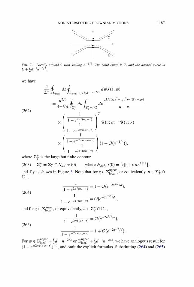
NONINTERSECTING BROWNIAN MOTIONS 1187
FIG. 7. Locally around 0 with scaling n−1/3. The solid curve is � and the dashed curve is� + i
2d−1n−2/3.
we haven
2π
∮�local
dz
∮�local+(i/2)d−1n−2/3
dwJ(z,w)
= n2/3
4π2id
∮�∗T
du
∮�∗T+i/2
dve1/2(τiu2−τj v2)−i(ξu−ηv)
u− v(262)
×⎛⎜⎝
1
1 − e2πi(nz−τ)1
1 − e−2πi(nz−τ)
⎞⎟⎠T
�(u;σ)−1�(v;σ)
×⎛⎜⎝
1
1 − e−2πi(nw−τ)−1
1 − e2πi(nw−τ)
⎞⎟⎠(
1 +O(n−1/4)),
where �∗T is the large but finite contour
�∗T =�T ∩Ndn1/12(0) where Ndn1/12(0)= {
z||z|< dn1/12},(263)
and �T is shown in Figure 3. Note that for z ∈�upperlocal , or equivalently, u ∈�∗
T ∩C+,
1
1 − e2πi(nz−τ) = 1 +O(e−2n2/3/d),
(264)1
1 − e−2πi(nz−τ) = O(e−2n2/3/d),
and for z ∈�lowerlocal , or equivalently, u ∈�∗
T ∩C−,
1
1 − e2πi(nz−τ) = O(e−2n2/3/d),
(265)1
1 − e−2πi(nz−τ) = 1 +O(e−2n2/3/d).
For w ∈�upperlocal + i
2d−1n−2/3 or�upper
local + i2d
−1n−2/3, we have analogous result for(1 − e±2πi(nw−τ))−1, and omit the explicit formulas. Substituting (264) and (265)

1188 K. LIECHTY AND D. WANG
and their counterparts for w into (262) and using the fact that det�(ζ ;σ)≡ 1, wefind that
n
2π
∮�local
dz
∮�local+(i/2)d−1n−2/3
dwJ(z,w)
= n2/3
4π2id
∮�∗T
du
∮�∗T+i/2
dve((τi/2)u2−(τj /2)v2)−i(ξu−ηv)
(266)
× f (u;σ)g(v;σ)− g(u;σ)f (v;σ)(u− v)
(1 +O
(n−1/4))
= n2/3
dK tacτi ,τj
(ξ, η)(1 +O
(n−1/4)),
where f (u;σ) and g(u;σ) are defined in (28).By the estimates of pn(z) and pn−1(z)/h
(T ;τ)n,n−1 in Proposition 3.7 and (176) in
Proposition 3.8, we have that for all z ∈� and w ∈� + i2d
−1n−2/3
pn(z)pn−1(w)− pn−1(z)pn(w)
h(T ;τ)n,n−1(z−w) = eng(z)+ng(w)−nlO(
n2/3),(267)
where g(z) is defined in (157) and the n2/3 factor comes from (z−w)−1. Hence,for all z ∈� and w ∈� + i
2d−1n−2/3,∣∣J (z,w)∣∣ = en(g(z)−(T /4)z2+πiz)+n(g(w)−(T /4)w2+πiw)en2/3d2(τiz
2−τjw2)
(268)× e−in1/3d(ξz−ηw)O
(n2/3),
where g is defined by g in (227). By direct calculation, we have that for z ∈ � \�local, Re(g(z)− T 2z2/4 + πiz) decreases as z moves away from 0. Hence, bystandard argument of steepest-descent method and the result of (266), we have that
Kti ,tj (x, y)=n
2π
∮�dz
∮�+(i/2)d−1n−2/3
dwJ(z,w)
= n
2π
∮�local
dz
∮�local+(i/2)d−1n−2/3
dwJ(z,w)+O(e−cn1/4)
(269)
= n2/3
dK tacτi ,τj
(ξ, η;σ)(1 +O(n−1/4)),
where c is a positive constant.At last,
◦W[i,j)(x, y) is defined in (112) with explicit formula given in (133). It
is 0 when tj ≤ ti and when tj > ti , a standard approximation technique gives that
◦W[i,j)(x, y)= n2/3
d
1√2π(τj − τi)
e−(η−ξ)2/(2(τj−τi ))(1 +O
(n−1/3)).(270)
Comparing (269) and (270) with (29) and (26), we prove (35).

NONINTERSECTING BROWNIAN MOTIONS 1189
5.4. Proof of Theorem 1.4. For notational simplicity, we only consider thelimiting 2-correlation functions, such that t1, t2 ∈ (0, T ) are two times and x, y aretwo locations on T. We assume that t1, t2, x, y are expressed by (31) with i = 1,j = 2, and then(
R(n)0→T
)ω(x;y; t1, t2)
(271)
= lim�x→0
1
(�x)2P
⎛⎝ there is a particle in [x, x +�x) at time t1,
there is a particle in [y, y +�x) at time t2,and the total winding number is ω
⎞⎠ .
From (135), we have
limn→∞
∑ω∈Z
(R(n)0→T
)ω(x;y; t1, t2)e2πω(τ+ε(n))i
(d
n3/4
)2
(272)
= limn→∞
Rn(T ; τ)Rn(T ; ε(n))R
(n)0→T (x;y; t1, t2; τ)
(d
n3/4
)2
,
where R(n)0→T (x;y; t1, t2; τ) is a special case of the τ -deformed joint correlationfunction defined in (115).
By the determinantal formula (116) and the asymptotic result (211), we havefor all τ ∈ [0,1],
limn→∞R
(n)0→T (x;y; t1, t2; τ)=
∣∣∣∣∣KPearcey−τ1,−τ1(ξ, ξ) K
Pearcey−τ2,−τ1(η, ξ)
KPearcey−τ1,−τ2(ξ, η) K
Pearcey−τ2,−τ2(η, η)
∣∣∣∣∣ ,(273)
and on the other hand by (184) and (24), we have
limn→∞
Rn(T ; τ)Rn(T ; ε(n))= limn→∞
∑ω∈Z
P(Total winding number equals ω)e2πω(τ+ε(n))i(274)
= ∑ω∈Z
qω2
√π
2Ke2πω(τ+ε(n))i .
Hence, a comparison of Fourier coefficients on both sides of (272) shows that
limn→∞
(R(n)0→T
)ω(x;y; t1, t2)
(d
n3/4
)2
(275)
= qω2
√π
2K
∣∣∣∣∣KPearcey−τ1,−τ1(ξ, ξ) K
Pearcey−τ2,−τ1(η, ξ)
KPearcey−τ1,−τ2(ξ, η) K
Pearcey−τ2,−τ2(η, η)
∣∣∣∣∣ ,which is the desired result. Thus, we prove Theorem 1.4 in the n= 2 case.

1190 K. LIECHTY AND D. WANG
6. Interpolation problem and Riemann–Hilbert problem associated to dis-crete Gaussian orthogonal polynomials.
6.1. Equilibrium measure and the g-function. In this subsection, we prove theresults presented in Section 3.1 for the supercritical case T > Tc. The existenceand uniqueness of the equilibrium measure associated to the potential T x2/2 thatsatisfies the minimization problem (137) and (138) is proved in Kuijlaars (2000),along with several analytic properties. Thus, if we find a probability measure νTwith continuous density function ρT (x) such that the associated g-function sat-isfies the variational condition (140), then it is the unique equilibrium measure.For T ≤ Tc = π2, it is straightforward to verify that the well-known semicirclelaw (142) and the g-function (157) satisfy the variational condition (140), so theequilibrium measure is given by (142). Thus, this subsection is dedicated to theconstruction of the equilibrium measure and the derivative of the g-function forT > Tc = π2. The g-function is then determined by its derivative up to the La-grange multiplier l. Our strategy is to construct a probability measure νT with con-tinuous density dνT (x)= ρT (x) dx together with the derivative of the associatedg-function, such that νT is supported on an interval [−β,β], and has a saturatedregion [−α,α], that is, ρT (x)= 0 for x ∈ R \ (−β,β), ρT (x)= 1 for x ∈ [−α,α]and 0 < ρT (x) < 1 for x ∈ (−β,α) ∪ (α,β), and then verify that the probabilitymeasure satisfies the variational condition (140). Therefore, we conclude that theconstruction of the equilibrium measure is valid.
The derivative of the g-function is expressed as
g′(z)=∫ β
−β1
z− x ρT (x) dx, z ∈ C \ [−β,β],(276)
and so the equilibrium measure νT = ρT (x)χ [−β,β](x) dx is given as
ρT (x)= −1
πImg′+(x)=
1
πImg′−(x) for x ∈ [−β,β],(277)
where g′+(x) and g′−(x) are the limiting values from the upper and lower half-planes, respectively. That the measure νT has total measure 1 is equivalent to
g′(z)= 1
z+O
(z−2) as z→ ∞.(278)
The variational problem (140) implies
g′+(x)+ g′−(x)= T x for x ∈ (−β,−α)∪ (α,β),(279)
g′+(x)− g′−(x)= −2πi for x ∈ (−α,α).(280)
To construct g′(z), we use the incomplete elliptic integrals F(z;k) and E(z;k)and the complete elliptic integrals K = K(k) and E = E(k) introduced in (144)
NONINTERSECTING BROWNIAN MOTIONS 1191
and (16). They have the properties that
F+(x;k)+ F−(x;k)= 2K, E+(x;k)+E−(x;k)= 2E(281)
for x ∈ (1, k−1),
F+(x;k)+ F−(x;k)= −2K, E+(x;k)+E−(x;k)= −2E(282)
for x ∈ (−k−1,−1),
F+(x;k)− F−(x;k)= 2iK′, E+(x;k)−E−(x;k)= 2i(K′ − E′)
(283)for x ∈ R \ (−k−1, k−1).
Here, we use the notation
K′ = K(k′), E′ = E
(k′)
where k′ =√
1 − k2.(284)
Identities (281) and (282) can be checked by straightforward computation, and(283) can be checked with the help of Gradshteyn and Ryzhik (2007), 3.152-9, page 280 and 3.169-17, page 209. The identity (283) also comes from theimaginary periods of F(z;k) and E(z;k); see Erdélyi et al. (1981), Section 13.7,page 314. For fixed α and β , let
k = α
β.(285)
With the help of Legendre’s relation [Erdélyi et al. (1981), Section 13.8, page 320,Formula (15)],
KE′ + K′E − KK′ = π
2,(286)
we find that when g′(z) is given by
g′(z)=
⎧⎪⎪⎨⎪⎪⎩T z
2+ 2EF
(z
α;k
)− 2KE
(z
α;k
)− πi, for z ∈C+,
T z
2+ 2EF
(z
α;k
)− 2KE
(z
α;k
)+ πi, for z ∈C−,
(287)
it satisfies (279) and (280), and it is also well defined on (−∞,−β) ∪ (β,∞) byanalytic continuation. To make (278) hold, we need to choose the correct valuesfor α and β . As z→ ∞, the asymptotic behaviors of F(z;k) and E(z;k) are
F(z;k)= iK′ + 1
kz+O
(z−2),(288)
E(z;k)= kz+ i(K′ − E′)+ k−1 − k2z
+O(z−2).(289)

1192 K. LIECHTY AND D. WANG
FIG. 8. The contours CR and C1,k−1 .
The constant term in (288) is obtained by
limz→∞z∈C+
F(z;k)=∫ i·∞
0
ds√(1 − s2)(1 − k2s2)
= i∫ ∞
0
dt√(1 + t2)(1 + k2t2)
(290)
= iF (1;√
1 − k2) = iK′,
where evaluation of the elliptic integral is done by Gradshteyn and Ryzhik (2007),3.152-2, page 279. The z−1 term in (288) follows the asymptotics of the integrandin the defining formula (144) of F(z;k). The z term in (289) is obvious, and theconstant term is given by
limz→∞z∈C+
E(z;k)− kz=∫ i·∞
0
(√1 − k2s2
1 − s2 − k)ds
(291)
= i
2
∫ ∞−∞
(√1 + k2t2
1 + t2 − k)dt.
To evaluate the integral on the right-hand side of (291), we define the pair of con-tours (see Figure 8),
CR = [−R,R] ∪ {Reiθ |θ ∈ [0, π]} counterclockwise,
C1,k−1 = contour starting from i, along the right-hand side of the(292)
imaginary axis, to k−1i, and then along the left-hand side
of the imaginary axis, back to i.

NONINTERSECTING BROWNIAN MOTIONS 1193
Then by the contour integral technique and Gradshteyn and Ryzhik (2007), 3.169-17, page 309,
∫ ∞−∞
√1 + k2t2
1 + t2 − k dt
= limR→∞
∮CR
√1 + k2t2
1 + t2 dt =∮C1,k−1
√1 + k2t2
1 + t2 dt
(293)
= 2∫ k−1
1
√1 − k2t2
1 − t2 dt
= 2(F(1;
√1 − k2
)−E(1;√
1 − k2)) = 2
(K′ − E′),
and we get the result. The z−1 term of (289) is obtained analogously to the z−1
term of (288).Then as z→ ∞ in C+,
g′(z)=(T
2− 2kK
α
)z+ 2i
(K′E + KE′ − KK′ − π
2
)(294)
+ 2α(
Ek
− (1 − k2)K2k
)1
z+O
(z−2).
Note that the constant term of g′(z) vanishes automatically by Legendre’s rela-tion (286). For k = α/β , the identity (278) is satisfied when α and β are given by(145) and (148).
By Lemma 3.2, the relation (148) is a 1–1 correspondence between T > Tc =π2 and k ∈ (0,1). Thus, for each T = T (k) > Tc, there are well-defined α,β andρT given by (145) and (278). By the construction of ρT , especially (279), we havethat the measure dνT with density ρT (x)χ [−β,β](x) has total measure 1, and sat-isfies the variational condition on [α,β] given that the Lagrange multiplier l isproperly chosen and 0 < ρT (x) < 1 for all x ∈ (α,β). By the symmetry of νTabout the origin, we finish the verification that νT is the equilibrium measure. Ad-ditionally, we have the following lemma, which states that the equilibrium measureis regular in the sense of Bleher and Liechty (2011).
LEMMA 6.1. (a) 0< ρT (x) < 1 for all x ∈ (α,β).(b) g+(x)+ g−(x)− T x2
2 − l > 0 for x ∈ [0, α).(c) 2g(x)− T x2
2 − l < 0 for x ∈ (β,∞).(d) There exist constants c1 and c2 such that
ρT (x)= c1√β − x(1 +O
((β − x))) as x→ β from the left(295)
1194 K. LIECHTY AND D. WANG
and
1 − ρT (x)= c2√x − α(1 +O
((x − α)))
(296)as x→ α from the right.
We finish this subsection by the proof of Lemmas 3.2 and 6.1.
PROOF OF LEMMA 3.2. The two limits in (149) are straightforward to checkfrom the integral formulas (16) of K and E. To see the monotonicity, we use Byrdand Friedman (1971), 710.00 and 710.02, page 282, and have
d
dk
(K(k)E(k)
) = E2 − (1 − k2)K2
k(1 − k2)(297)
= 1
k(1 − k2)
∫ 1
0
√1 − k2s2 − √
1 − k2√(1 − s2)(1 − k2s2)
ds > 0,
which proves the monotonicity. �
PROOF OF LEMMA 6.1. For part (a), since ρT (x) on (0, α) is expressed by�0(x;k) for x ∈ (0,1) in (151), we only need to show that �0(x;k) ∈ (0,1)for x ∈ (0,1). By Byrd and Friedman (1971), 151.01, page 36, we have that�0(0;k) = 0 and �0(1;k) = 1. We need only to show that �0(x;k) is strictlyincreasing on (0,1). By Byrd and Friedman (1971), 730.04, page 284, this is im-plied by the inequality E − (1 − k2)x2K > 0 for all x ∈ (0,1). The inequality isproved as
E − (1 − k2)x2K =
∫ 1
0
√1 − k2s2 − x2
√1 − k2√
(1 − s2)(1 − k2s2)> 0.(298)
For parts (b) and (c), we note that since g+(x) + g−(x) − T x2/2 − l, whichbecomes 2g(x)− T x2/2 − l for x > β , is a continuous function and l is chosen sothat it vanishes for x ∈ [α,β], it suffices to show the inequalities
1
4
(g′+(x)+ g′−(x)− T x
) = EF(x
α;k
)− KE
(x
α;k
)< 0,
(299)x ∈ (0, α),
1
4
(2g′(x)− T x) = −E
∫ x/α
k−1
ds√(s2 − 1)(k2s2 − 1)
(300)
− K∫ x/α
k−1
√k2s2 − 1√s2 − 1
ds < 0, x ∈ (β,∞).

NONINTERSECTING BROWNIAN MOTIONS 1195
The inequality (300) obviously holds. To prove (299), we use Byrd and Friedman(1971), 414.01, page 229,
EF(x
α;k
)− KE
(x
α;k
)
= 1
βx
√(β − x2
)(α2 − x2
)(K −�1
(−x
2
β2 ;k))
(301)
= −1
βx
√(β − x2
)(α2 − x2
) ∫ 1
0
(x2/β2)s2 ds
(1 − (x2/β2)s2)√(1 − s2)(1 − k2s2)
,
which is clearly negative for x ∈ (0, α).Part (d) is easy to check using formula (150). �
6.2. Interpolation problem and outline of the steepest descent analysis. Theorthogonal polynomials (90) are encoded in the following interpolation prob-lem (IP). For a given n = 0,1, . . . , find a 2 × 2 matrix-valued function Pn(z) =(Pn(z)ij )1≤i,j≤2 with the following properties:
1. Analyticity: Pn(z) is an analytic function of z for z ∈ C \Ln,τ .2. Residues at poles: At each node x ∈ Ln,τ , the elements Pn(z)11 and Pn(z)21
of the matrix Pn(z) are analytic functions of z, and the elements Pn(z)12 andPn(z)22 have a simple pole with the residues,
Resz=x Pn(z)j2 = 1
ne−nT x2/2Pn(x)j1, j = 1,2.(302)
3. Asymptotics at infinity: There exists a function r(x) > 0 on Ln,τ such that
limx→∞ r(x)= 0,(303)
and such that as z→ ∞, Pn(z) admits the asymptotic expansion,
Pn(z)∼(I + P1
z+ P2
z2 + · · ·)(zn 00 z−n
),
(304)
z ∈ C∖[ ∞⋃
x∈Ln,τD(x, r(x)
)],
where D(x, r(x)) denotes a disk of radius r(x) > 0 centered at x and I is theidentity matrix.
The unique solution to the IP is
Pn(z)=(
p(T ;τ)n,n (z)
(Cp
(T ;τ)n,n
)(z)(
h(T ;τ)n,n−1
)−1p(T ;τ)n,n−1(z)
(h(T ;τ)n,n−1
)−1(Cp
(T ;τ)n,n−1
)(z)
),(305)

1196 K. LIECHTY AND D. WANG
where the weighted discrete Cauchy transform C is defined in (162). The nor-malizing constants in (92) and the recurrence coefficients (93) are encoded in thematrices P1 and P2 in the expansion (304). Namely, we have
h(T ;τ)n,n = [P1]12,
(h(T ;τ)n,n−1
)−1 = [P1]21(306)
and
β(T ;τ)n,n−1 = [P2]21
[P1]21− [P1]11.(307)
The steepest descent analysis of the IP for a general class of orthogonal poly-nomials is described in Bleher and Liechty (2011) in the case τ = 0 [see alsoBaik et al. (2007) for polynomials orthogonal on a finite lattice]. For the discreteGaussian orthogonal polynomials the analysis for a general τ was given in Liechty(2012) for the case T = Tc + o(1) as n→ ∞. The analysis consists of a sequenceof transformations
Pn → Rn → Tn → Sn → Xn.(308)
The first transformation Pn → Rn reduces the IP to a Riemann–Hilbert problem(RHP). The second transformation Rn → Tn uses the g-function to give a RHPwhich approaches the identity matrix as z→ ∞. The third transformation Tn →Sn is local and involves transformations only close to the support of the equilibriummeasure. The RHP for Sn can be approximated by RHPs for which we can writeexplicit solutions in different regions of the complex plane, and Xn is uniformlyclose to the identity matrix.
In the supercritical case T > Tc, one can make the reduction to a RHP in thefollowing way. Fix some ε > 0 and some 0 < δ < 1. Let �+ (resp., �−) be acontour from ei0 · ∞ to eiπ · ∞ (resp., e−iπ · ∞ to ei0 · ∞) which lies in the upper(resp., lower) half-plane and sits at a distance εn−δ from the real line except closeto the turning points ±α and ±β , where it maintains a fixed distance ε from thesepoints; see Figure 9. We let �± be the region bounded by the real line and �± with|Re z|< α, and ∇± the region bounded by the real line and �± with |Re z|> α.We make the reduction of the IP to a RHP and the transformations to the RHP as inLiechty (2012); see Liechty (2012), Figure 2 and equations (4.27), (4.28), (4.32).
FIG. 9. The contour �S . The horizontal line is R and the vertical segments pass through ±α and±β . The remaining pieces of the contour are �± which pass close to R at a distance of εn−δ exceptclose to the turning points ±α and ±β . The regions �± are bounded by the real line and �± with
|Re z|< α, and the regions ∇± are bounded by the real line and �± with |Re z|> α.

NONINTERSECTING BROWNIAN MOTIONS 1197
Note that the lattice shift parameter which we call τ is called (−α) in Liechty(2012).
Let us briefly describe the explicit transformations involved in the steepest de-scent analysis. Introduce the functions
�(z) := sin(nπz− τπ)nπ
, G(z) := g+(x)− g−(z),(309)
where g±(z) are defined first on R as the limiting values of the g-function fromC±, and then extended to a small neighborhood of R by analytic continuation.Notice that the function G(z) is also given by the integral formula (141). Thetransformations described above involve the matrices
Du±(z)=⎛⎝1 −e
−(nT /2)z2
n�(z)e±iπ(nz−τ)
0 1
⎞⎠ ,
Dl±(z)=(
�(z)−1 0
−ne(nT /2)z2e±iπ(nz−τ) �(z)
),
(310)
j±(z)=(
1 0e∓nG(z) 1
),
A±(z)=⎛⎝∓ 1
2nπie∓iπ(nz−τ) 0
0 ∓2nπie±iπ(nz−τ)
⎞⎠ .
After the first two transformations of the IP, the matrix Sn(z) is defined as
Sn(z)=
⎧⎪⎪⎪⎪⎪⎪⎪⎪⎪⎪⎪⎪⎪⎪⎪⎪⎪⎪⎪⎪⎪⎪⎪⎪⎪⎪⎪⎪⎪⎪⎪⎨⎪⎪⎪⎪⎪⎪⎪⎪⎪⎪⎪⎪⎪⎪⎪⎪⎪⎪⎪⎪⎪⎪⎪⎪⎪⎪⎪⎪⎪⎪⎪⎩
e−(nl/2)σ3
(1 00 −2πi
)Pn(z)Dl±(z)
(1 00 −2πi
)−1
× e−n(g(z)−l/2)σ3A±(z),for z ∈ �±,
e−(nl/2)σ3
(1 00 −2πi
)Pn(z)Du±(z)
(1 00 −2πi
)−1
× e−n(g(z)−l/2)σ3j±(z)∓1,
for z ∈ ∇± and α ≤ |Re z| ≤ β,e−(nl/2)σ3
(1 00 −2πi
)Pn(z)Du±(z)
(1 00 −2πi
)−1
× e−n(g(z)−l/2)σ3,
for z ∈ ∇± and |Re z| ≥ β,e−(nl/2)σ3
(1 00 −2πi
)Pn(z)
(1 00 −2πi
)−1
e−n(g(z)−l/2)σ3,
otherwise,
(311)
where σ3 = (10
0−1
)is the third Pauli matrix. This matrix function satisfies the
following RHP.

1198 K. LIECHTY AND D. WANG
• Sn(z) is an analytic function of z for z ∈ C \ �S , where �S consists R, �+,and �−, along with the four vertical segments [±β − iε,±β + iε] and [±α −iε,±α+ iε], oriented as shown in Figure 9.
• For z ∈�S , the function Sn(z) satisfies the jump conditions
Sn+(z)= Sn−(z)jS(z),(312)
where
jS(z)=
⎧⎪⎪⎪⎪⎪⎪⎪⎪⎪⎪⎨⎪⎪⎪⎪⎪⎪⎪⎪⎪⎪⎩
(0 1
−1 0
), for z ∈ (−β,−α)∪ (α,β),(
e−i n 0O(e−n1−δc(z)) ei n
), for z ∈ (−α,α),(
1 O(e−n1−δc(z))
O(e−n1−δc(z)) 1
),
for z on the rest of �S,
(313)
where
n := π(n+ 1 − 2τ),(314)
and c(z) is a nonnegative continuous function on �S which may vanish only atthe turning points ±α and ±β .
• As z→ ∞,
Sn(z)= I + S1
z+ S2
z2 + · · · .(315)
Notice that the errors in the off diagonal terms in (313) are subexponential, but stillsmaller than any power of n. In the usual method of steepest descent [Bleher andLiechty (2011)], these terms are exponentially small, but our analysis is slightlydifferent in that we have taken the contours �± to be very close to R. The reason isthat in Proposition 3.6 the asymptotic formulas are given for z ∈D(δ, ε, n), whichis the region above �+ and below �−.
6.2.1. Model RHP. The model RHP appears when we drop in the jump matrixjS(z) the terms that vanish as n→ ∞:
• M(z) is analytic in C \ [−β,β].• M+(z)= M−(z)jM(z) for z ∈ [−β,β], where
jM(z)=
⎧⎪⎪⎨⎪⎪⎩
(0 1
−1 0
), z ∈ (−β,−α)∪ (α,β),(
e−i n, 00 ei n
), z ∈ (−α,α).
(316)
• As z→ ∞,
M(z)∼ I + M1
z+ M2
z2 + · · · .(317)

NONINTERSECTING BROWNIAN MOTIONS 1199
The solution to this RHP is described in terms of Jacobi theta functions, and ispresented in Bleher and Liechty (2010), Section 8.
Consider the function u(z) defined in (165). This function is analytic for z ∈C \ [−β,β]. On that interval it satisfies certain jump conditions [see Bleher andLiechty (2010), Section 8]. We will use the Jacobi theta functions ϑj (z), (j = 3,4)with elliptic nome q given by (21). The solution is slightly different for n odd andn even. Using the notation ε(n) introduced in (4), we can write the solution in thefollowing uniform way:
M(z)= F(∞)−1
⎛⎜⎜⎜⎝γ (z)+ γ−1(z)
2
ϑ3(u(z)− π/4 − π(τ − ε(n)))ϑ3(u(z)− π/4)
γ (z)− γ−1(z)
2i
ϑ3(u(z)+ π/4 − π(τ − ε(n)))ϑ3(u(z)+ π/4)(318)
γ (z)− γ−1(z)
−2i
ϑ3(u(z)+ π/4 + π(τ − ε(n)))ϑ3(u(z)+ π/4)
γ (z)+ γ−1(z)
2
ϑ3(u(z)− π/4 + π(τ − ε(n)))ϑ3(u(z)− π/4)
⎞⎟⎟⎟⎠ ,
where
F(∞)=
⎛⎜⎜⎝ϑ3(π(τ − ε(n)))
ϑ3(0)0
0ϑ3(π(τ − ε(n)))
ϑ3(0)
⎞⎟⎟⎠ .(319)
The entries of the matrix(1 00 −2πi
)−1
M(z)(
1 00 −2πi
),(320)
are listed in (169)–(172). Notice that the ratios of theta functions in (318) and(319) become trivial when τ = ε(n). The coefficient M1 in the expansion of M(z)at z= ∞ is
M1 =
⎛⎜⎜⎜⎝
πβϑ ′3(π(τ − ε(n)))
4Kϑ3(π(τ − ε(n))) −β − α2i
ϑ3(0)ϑ4(π(τ − ε(n)))ϑ4(0)ϑ3(π(τ − ε(n)))
β − α2i
ϑ3(0)ϑ4(π(τ − ε(n)))ϑ4(0)ϑ3(π(τ − ε(n))) −πβϑ
′3(π(τ − ε(n)))
4Kϑ3(π(τ − ε(n)))
⎞⎟⎟⎟⎠ ,(321)
and the (21)-entry of the coefficient M2 is
[M2]21 = πβ(β − α)ϑ3(0)ϑ ′4(π(τ − ε(n)))
8iϑ3(π(τ − ε(n)))ϑ4(0)K.(322)
Notice that according the RHP for M(z), det M(z) is entire. Since det M(∞)=1, it follows from Liouville’s theorem that det M(z)≡ 1.

1200 K. LIECHTY AND D. WANG
6.2.2. The local solution at ±α and ±β . Consider small disks D(±α, ε) andD(±β, ε) around ±α and ±β with radius ε. We seek a local parametrix U(z) inthese disks satisfying:
• U(z) is analytic in {D(±α, ε)∪D(±β, ε)} \�S .• For z ∈ {D(±α, ε)∪D(±β, ε)}∩�S , U(z) satisfies the jump condition U+(z)=
U−(z)jS(z).• On the boundary of the disks, U(z) satisfies
U(z)= M(z)(I +O
(n−1)), z ∈ ∂D(±α, ε)∪ ∂D(±β, ε).(323)
The solution is given explicitly in terms of Airy functions, and we do not describeit here.
6.2.3. The final transformation of the RHP. We now consider the contour �X ,which consists of the circles ∂D(±β, ε) and ∂D(±α, ε), all oriented counterclock-wise, together with the parts of �S \ {[−β,α] ∪ [α,β]} which lie outside of thedisks D(±β, ε), D(±α, ε). Let
Xn(z)(324)
={
Sn(z)M(z)−1, for z outside the disks D(±β, ε),D(±α, ε),Sn(z)U(z)−1, for z inside the disks D(±β, ε),D(±α, ε).
Then Xn(z) satisfies a RHP with jumps on the contour �X which are uniformlyclose to the identity matrix, and Xn(∞) = I . The solution to this RHP is givenexplicitly in terms of a Neumann series. Due to the fact that the contours �± andthe real line are very close to one another (at a distance of the order n−δ), we findthat Xn(z) satisfies
Xn(z)∼ I +O(
1
n1−δ(|z| + 1)
)as n→ ∞,(325)
uniformly for z ∈ C \�X , which is a weaker error than the O(n−1) error in Bleherand Liechty (2011).
6.3. Proofs of Propositions 3.6, 3.9 and 3.10. We can invert the explicittransformations of the IP in different regions of the complex plane using (324)and (311). The asymptotic formula (325) then gives asymptotic formulas forPn(z). Considering z in the region D(δ, ε, n) proves Proposition 3.6. Consideringz ∈ E(ε), and taking δ = 0 proves Proposition 3.9. For Proposition 3.10, we caninvert the explicit transformations with δ = 0, and Proposition 3.10 then followsfrom (306), (307), and the expansions of M(z) at z= ∞ given in (321) and (322).
NONINTERSECTING BROWNIAN MOTIONS 1201
APPENDIX A: CONSTRUCTION OF STEEPEST-DESCENT CONTOURS �AND �
In this appendix, we show that the first and second derivatives of I (z), definedin (225), vanish at z= 0, and construct two contours � and � lying in the regionC+ = {z ∈ C| Im z≥ 0} and passing through 0, such that � is from e0 ·∞ to eπi ·∞and � is from M to −M where M > β . We require that Re I (z) attains its uniqueglobal maximum on � at 0, and attains its unique global minimum on � at 0. SinceRe I (z) is symmetric about the imaginary axis, we only need to construct � ∩Dand � ∩D where
D = {z ∈ C|Re z≥ 0 and Im z≥ 0}(326)
and construct the other parts of them by reflection.To simplify the notation, we take a change of variable
u= z
α.(327)
Then we have that, by (156), (225) and (287) [Byrd and Friedman (1971), 140.01,page 33]
I ′(z)= −2K(Z(u)−
(1 − E
K
)u
)(328)
where Z(u)= Z(u;k)=E(u;k)− EKF(u;k).
REMARK A.1. Here, the arguments of Z(u;k), the Jacobi Zeta function, aredifferent from those in Byrd and Friedman (1971) such that our u is equal to sinβfor the β in Z(β, k) in Byrd and Friedman (1971), 140.02, 03. The Jacobi Zetafunction also appears in (199), where the arguments have same meaning as thosein Byrd and Friedman (1971), 140.01, but the parameter is k instead of k.
Below we collect some results about Z(u).
LEMMA A.1. (a) Z(u) is analytic in D,
Z′(0)= 1 − EK,Z′′(0)= 0 and Z(u)= ku− πi
2K+O
(u−1)
(329)as u→ ∞ in D.
(b) For x ∈ [0,1], Z(x) is a real-valued function such that
Z(0)= Z(1)= 0 and Z′′(x) < 0 for all u ∈ (0,1).(330)
1202 K. LIECHTY AND D. WANG
(c) For x ∈ [1, k−1], Z(x) is a pure imaginary-valued function such that
ImZ(1)= 0, ImZ(
1
k
)= − π
2Kand
d
dxImZ(x) < 0
(331)
for all x ∈(
1,1
k
).
(d) For x ∈ [k−1,∞), Z(x)+ πi/(2K) is a real-valued function such that
Z
(1
k
)+ πi
2K= 0 and
d
dx
(Z(x)+ πi
2K
)> 0,
(332)d2
dx2
(Z(x)+ πi
2K
)< 0 for all x ∈
(1
k,∞
).
(e) For y ∈ [0,∞), Z(iy) is a pure imaginary-valued function such that
Z(0)= 0 andd
dyImZ(iy) > 0,
d2
dy2 ImZ(iy) > 0
(333)for all y ∈ (0,∞).
PROOF. The linear term in the asymptotics in part (a) of Lemma A.1 is a directconsequence of the explicit formula of Z(u) in D,
Z(u)=∫ u
0
(1 − E/K)− k2s2√(1 − s2)(1 − k2s2)
,(334)
which is given by (328) and (144). In the integrand of (334) the sign of the squareroot is chosen as
√(1 − s2)(1 − k2s2)∼ 1 as s approaches 0 from the regionD. To
compute the constant term, it suffices to compute the asymptotics of Z(iy)− iky =E(iy;k)− (E/K)F (iy;k)− iky as y→ +∞. By Gradshteyn and Ryzhik (2007),3.152-1, page 279, limy→∞F(iy;k)= iK′, and by the computation in equations(291) and (293), limy→∞E(iy;k) − iky = i(K′ − E′). Then an application ofLegendre’s relation (286) yields the result.
From the formula (334), it is clear that: Z(0) = 0; Z(x) is real valued for x ∈[0,1]; ReZ(x) is constant for x ∈ [1, k−1]; ImZ(x) is constant for x ∈ [k−1,∞);and Z(iy) is pure imaginary for y ∈ [0,∞). It is also straightforward to see that
Z(1)=E(1;k)− EKF(1;k)= E − E
KK = 0,(335)
and with the help of Byrd and Friedman (1971), 111.09, page 11, and the Legen-dre’s relation (286),
Z(k−1) = E(k−1;k)− E
KF(k−1;k) = E + i(K′ − E′)− E
K
(K + iK′)
(336)
= i
K
(KK′ − KE′ − EK′) = − πi
2K.

NONINTERSECTING BROWNIAN MOTIONS 1203
Thus, all the identities in (330), (331), (332), (333) are all proved.To consider the values of Z′(0) and Z′′(0), and the inequalities of Z′(u) in
(331), (332), (333), we write from (334)
Z′(u)= (1 − E/K)− k2u2√(1 − u2)(1 − k2u2)
ds.(337)
Note that for u≥ 1,(1 − E
K
)− k2u2 = 1
K
∫ 1
0
k2(s2 − u2)√(1 − s2)(1 − k2s2)
ds < 0,(338)
we obtain the inequality parts of (331), (332), (333) and the evaluation of Z′(0)and Z′′(0) in (329).
To consider the inequalities of Z′′(u) in (330), (332) and (333), we can writeZ′(u) as
Z′(u)= k
K
√1 − u2
k−2 − u2
∫ 1
0
(s2 − u2)/(1 − u2)√(1 − s2)(1 − k2s2)
ds,(339)
for u ∈ (0,1) and u ∈ (k−1,∞), where in either case the square root is takenpositive value. We observe that Z′(u) is a decreasing function on (0,1) since(1−u2)/(k−2 −u2) and (s2 −u2)/(1−u2) are both increasing, while Z′(u) is alsoa decreasing function on (k−1,∞) by exactly the same reason. Similarly, writing
d
dyImZ(iy)= k
K
√1 + y2k−2 + y2
∫ 1
0
(s2 + y2)/(1 + y2)√(1 + s2)(1 + k2s2)
ds,(340)
we observe that ddy
ImZ(iy) is increasing for all y ∈ (0,∞). This proves the in-equality of Z′′(u) in (330), (332) and (333). �
LEMMA A.2. The function I ′(z) has only one zero z= 0 in the region D thatis a third-order zero, and I (4)(0) > 0.
PROOF. From (329), it is clear that u = 0 is a zero of Z(u) − (1 − E/F)uwith order at least 3, and then by (328) the same holds for I ′(z). On the otherhand, I (4)(z) = g(4)(z), and the explicit computation (236) of g(4)(0) shows thatI (4)(0) > 0. Below we show that the function Z(u)− (1 − E/F)u has only onezero u= 0 in D, and complete the proof.
We note that by the results in Lemma A.1, Z(u)− (1 − E/F)u has no zero ineither {z = x|x > 0} or {z = iy|y > 0}, and it does not vanish as u→ ∞. So toprove that Z(u) − (1 − E/F)u has no other zero in D, we define a region (seeFigure 10)
DR(1)= {u ∈D||u| ≤R} \ {u ∈ C|Reu < 1 and Imu < R−1},(341)

1204 K. LIECHTY AND D. WANG
FIG. 10. The region DR(1).
where R is a positive number, and need only to show that for however large R,Z(u)− (1 − E/K)u has no zero in the interior of DR(1).
By the results in Lemma A.1, we have that if R is large enough, then Z is ahomeomorphic mapping on ∂DR(1). Then by a basis result for univalent functions,Z maps the interior ofDR(1) into the region enclosed by Z(∂DR(1)) that does notcontain 0, see Figure 11. Then by a continuity argument, if Z(u)− (1 − E/K)uhas a zero in the interior of DR(1), there must be a t ∈ (0,1 − E/K) such thatZ(u)− tu has a zero on ∂DR(1), but by the results in Lemma A.1, for all such t ,Z(u) − tu does not vanish on ∂DR(1) given that R is large enough. Thus, weshow that Z(u) − (1 − E/K)u has no zero other than 0 in D by contradiction.
�
Now we construct �. By (329) and (330), we know that Re(Z(u)− (1−E/K)u)is decreasing on [0,1]. By Lemma A.1(c) and that (1 − E/K) > 0, we also havethat Re(Z(u) − (1 − E/K)u) is decreasing on [1, k−1]. By the relation (328),Re I (z) is decreasing on the interval [0, β]. Thus, it suffices to define � ∩D as the
FIG. 11. The shape of Z(∂DR(1)) with k = 0.9 and R = 7.

NONINTERSECTING BROWNIAN MOTIONS 1205
FIG. 12. Schematic graphs of � and � in D.
interval [0, β] if we allow M = β . Practically, for the convenience of the asymp-totic analysis in Section 5.2, we let M be slightly bigger than β and define � ∩Dby a deformation of the interval [0,M] such that [0, α/2] is part of � ∩ D and(α/2,M) is lifted above slightly; see Figure 12.
In the construction of � ∩D and �∩D, we use techniques in planar dynamicalsystems. Regarding Re I (z) as a function defined on the Cartesian plane whosecoordinates are Re z and Im z, we define the gradient field
∇ Re I (z)=(∂
∂xRe I (z),
∂
∂yRe I (z)
)(342)
where x = Re z, y = Im z.
By Lemma A.1(a), (e), we have that for y > 0, Z(iy) − (1 − E/K)iy is pureimaginary, and its imaginary part is positive. Then by (328), we conclude that{iy|y > 0} is an upward flow curve of ∇ Re I (z). By Lemma A.1(d) and the rela-tion (328), we have that for all x >M > β , Im(Z(x)− (1 − E/K)x > 0 and thenthe gradient field ∇ Re I (z) is transversal to the interval [M,∞) and is outwardof D.
Since by Lemma A.2, 0 is a triple zero of I ′(z) and I (4)(0) > 0, there is aflow curve that ends at 0, with direction π/4, and we denote it as γ . Since thegradient field ∇ Re I (z) has no singular point by Lemma A.2, this flow curve isfrom either the boundary of D or ∞. As we showed above, the left edge of Dis a flow curve and at the interval [M,∞), as part of ∂D, the gradient field isoutward, so the γ cannot be from the left edge ofD or [M,∞). If γ is from (0,M),then it crosses � at a point other than 0, denoted by z0. But by the definition of�, Re I (z0) > Re I (0). On the other hand, by the property of the flow curve γ ,Re I (z0) < Re I (0), and we derive a contradiction. Thus, γ cannot be from ∂D,but is from ∞. At last by the behavior of ∇ Re I (z) given in Lemma A.1(a), weverify that it suffices to let � ∩D = γ , as shown in Figure 12.
1206 K. LIECHTY AND D. WANG
APPENDIX B: PROOF OF PROPOSITION 1.5
Since �(ζ ; s) satisfies [Hastings and McLeod (1980)]
∂
∂s�(ζ ; s)=
(−iζ q(s)
q(s) iζ
)�(ζ ; s),(343)
it is easy to derive the identity that for u, v ∈�T ,
∂
∂s
(f (u; s)g(v; s)− g(u; s)f (v; s)
u− v)
(344)= −i(f (u; s)g(v; s)+ g(u; s)f (v; s)),
where f and g are defined by � by (28). Hence, (30) can be written as
K tacτi ,τj
(ξ, η;σ)= 1
4π2
∫�T
du
∫�T
dveτiu2/2−τj v2/2e−i(uξ−vη)
×∫ ∞σds
(f (u; s)g(v; s)+ g(u; s)f (v; s))
=∫ ∞σds
[(1
2π
∮�T
dueτiu2/2−iξuf (u; s)
)(345)
×(
1
2π
∮�T
dve−τiv2/2+iηvg(v; s))
+(
1
2π
∮�T
dueτiu2/2−iξug(u; s)
)
×(
1
2π
∮�T
dve−τiv2/2+iηvf (v; s))].
In order to relate formula (345) for the tacnode kernel to the other formula (45)defined by Airy function and related operators, we consider the expressions forthe entries of �(ζ ; s) in terms of Airy functions. Introduce the functions in x withparameters ζ and s,
E+(x)= E+(x; ζ, s) := ei((4/3)ζ 3+(s+2x)ζ ),(346)
E−(x)= E−(x; ζ, s) := e−i((4/3)ζ 3+(s+2x)ζ ) =E+(x;−ζ, s).Then the matrix entries of �(ζ ; s) are given by the formulas
11(ζ ; s)= 〈E−,Rs + δ0〉0, 21(ζ ; s)= −〈E−,Qs〉0,(347)
12(ζ ; s)= −〈E+,Qs〉0, 22(ζ ; s)= 〈E+,Rs + δ0〉0,(348)
where the inner product 〈·, ·〉0, functions Rs , Qs , and the delta function δ0 are de-fined in Section 1.2. The derivation of (347) is essentially given in Baik, Liechtyand Schehr (2012). Note that the functions �1(ζ ; s) and �2(ζ ; s) in Baik, Liechty

NONINTERSECTING BROWNIAN MOTIONS 1207
and Schehr (2012), Proposition 2.1, are the same as the functions �1(ζ ; s) and�2(ζ ; s) in Claeys and Kuijlaars (2006), and the entries 11(ζ ; s) and 21(ζ ; s)are the same as the functions�1(ζ ; s) and�2(ζ ; s) in Claeys and Kuijlaars (2006).Using the relation given in equation (1.19) of Claeys and Kuijlaars (2006), equa-tion (347) follows from Proposition 2.1 of Baik, Liechty and Schehr (2012). Bythe relation (15), (347) implies (348).
Consider now the integrals
I±a,b;s(x) :=
1
2π
∮�±T
eaζ2+ibζE±(x; ζ, s) dζ,(349)
where�+T (resp.,�−
T ) is the connected piece of�T which lies above (resp., below)the real axis. A simple change of variables gives that
I+a,b;s(x)=
1
2π
∮�+T
ei(4/3)ζ3+aζ 2+i(s+2x+b)ζ dζ
(350)
= −2−2/3e−a3/24−a(s+2x+b)/4Ai(s + 2x + b
22/3 + a2
28/3
),
where we have used the integral representation of the Airy function
Ai(x)= −1
2π
∮�+T
e(i/3)ζ3+ixζ dζ.(351)
Similarly,
I−a,b;s(x)= 2−2/3e−a3/24−a(s+2x−b)/4Ai
(s + 2x − b
22/3 + a2
28/3
).(352)
We can now write the expression (345) in terms of Airy functions and operatorsonly, since the functions f and g there are expressed by entries of � . Notice thatin the expressions (347) and (348) for the entries of the matrix � , the dependenceon ζ lies solely in the left-hand side of the inner products. Thus, by changing theorder of integration, we can write (345) in terms of the integrals I±
a,b;s(x). Indeedwe have
K tacτi ,τj
(ξ, η;σ)=∫ ∞σds
[(⟨I−τi/2,−ξ ;s,Rs + δ0⟩0 + ⟨
I+τi/2,−ξ ;s,Qs
⟩0
)× (−⟨
I+−τj /2,η;s,Rs + δ0⟩0 − ⟨
I−−τj /2,η;s,Qs
⟩0
)(353)
+ (−⟨I+τi/2,−ξ ;s,Rs + δ0⟩0 − ⟨
I−τi/2,−ξ ;s,Qs
⟩0
)× (⟨
I−−τj /2,η;s,Rs + δ0⟩0 + ⟨
I+−τj /2,η;s,Qs
⟩0
)].
Notice that in terms of the function bτ,z,σ defined in (43),
I+τ,z;s(x)= −2−2/3πb2−4/3τ,2−2/3z,s(x),
(354)I−τ,z;s(x)= 2−2/3πb2−4/3τ,−2−2/3z,s(x).

1208 K. LIECHTY AND D. WANG
Hence, formula (353) becomes
K tacτi ,τj
(ξ, η;σ)
= 2−4/3∫ ∞σds
[(〈b2−7/3τi ,2−2/3ξ,s,Rs + δ0〉0 − 〈b2−7/3τi ,−2−2/3ξ,s,Qs〉0)
× (〈b−2−7/3τj ,2−2/3η,s,Rs + δ0〉0
− 〈b−2−7/3τj ,−2−2/3η,s,Qs〉0)
(355)
+ (〈b2−7/3τi ,−2−2/3ξ,s,Rs + δ0〉0 − 〈b2−7/3τi ,2−2/3ξ,s,Qs〉0)
× (〈b−2−7/3τj ,−2−2/3η,s,Rs + δ0〉0
− 〈b−2−7/3τj ,2−2/3η,s,Qs〉0)],
which is, in terms of the function p1(z; s, τ ) defined in (46),
K tacτi ,τj
(ξ, η;σ)
= 2−4/3∫ ∞σds
(p1
(−2−2/3ξ ; s,2−7/3τi)p1
(−2−2/3η; s,−2−7/3τj)
(356)+ p1
(2−2/3ξ ; s,2−7/3τi
)p1
(2−2/3η; s,−2−7/3τj
))= 2−2/3Ltac
(2−2/3ξ,2−2/3η;σ,2−7/3τi,2
−7/3τj),
where Ltac is defined in (44). It is simple to see that by (26)
2−2/3(φ2·2−7/3τi ,2·2−7/3τj
(2−2/3ξ,2−2/3η
)) = φτi,τj (ξ, η).(357)
Combining (355) and (357) gives (47), and Proposition 1.5 is proved.
Acknowledgments. Part of this work was carried out during the workshopRandom matrices and applications at the University of Michigan in June 2013. Theauthors thank the organizers of that conference, Jinho Baik and Raj Rao Nadaku-diti, and also thank Jinho Baik and Arno Kuijlaars for helpful comments. Theauthors also thank Grégory Schehr for discussions and for pointing out the recentpreprint Castillo and Dupic (2014). D. Wang thanks Peter Forrester for discussionon the relation to Yang–Mills theory, as well as Wexiao Shen and Rongfeng Sun.
REFERENCES
ADLER, M., FERRARI, P. L. and VAN MOERBEKE, P. (2013). Nonintersecting random walks in theneighborhood of a symmetric tacnode. Ann. Probab. 41 2599–2647. MR3112926
ADLER, M., JOHANSSON, K. and VAN MOERBEKE, P. (2014). Double Aztec diamonds and thetacnode process. Adv. Math. 252 518–571. MR3144240
ADLER, M., ORANTIN, N. and VAN MOERBEKE, P. (2010). Universality for the Pearcey process.Phys. D 239 924–941. MR2639611
NONINTERSECTING BROWNIAN MOTIONS 1209
ADLER, M. and VAN MOERBEKE, P. (2005). PDEs for the joint distributions of the Dyson, Airy andsine processes. Ann. Probab. 33 1326–1361. MR2150191
ADLER, M., VAN MOERBEKE, P. and WANG, D. (2013). Random matrix minor processes relatedto percolation theory. Random Matrices Theory Appl. 2 1350008, 72. MR3149438
APTEKAREV, A. I., BLEHER, P. M. and KUIJLAARS, A. B. J. (2005). Large n limit of Gaussianrandom matrices with external source. II. Comm. Math. Phys. 259 367–389. MR2172687
BAIK, J., LIECHTY, K. and SCHEHR, G. (2012). On the joint distribution of the maximum and itsposition of the Airy2 process minus a parabola. J. Math. Phys. 53 083303, 13. MR3012644
BAIK, J. and SUIDAN, T. M. (2007). Random matrix central limit theorems for nonintersectingrandom walks. Ann. Probab. 35 1807–1834. MR2349576
BAIK, J., KRIECHERBAUER, T., MCLAUGHLIN, K. T.-R. and MILLER, P. D. (2007). Discrete Or-thogonal Polynomials: Asymptotics and Applications. Annals of Mathematics Studies 164. Prince-ton Univ. Press, Princeton, NJ. MR2283089
BLEHER, P. and KUIJLAARS, A. B. J. (2004). Large n limit of Gaussian random matrices withexternal source. I. Comm. Math. Phys. 252 43–76. MR2103904
BLEHER, P. M. and KUIJLAARS, A. B. J. (2007). Large n limit of Gaussian random matrices withexternal source. III. Double scaling limit. Comm. Math. Phys. 270 481–517. MR2276453
BLEHER, P. and LIECHTY, K. (2010). Exact solution of the six-vertex model with domain wallboundary conditions: Antiferroelectric phase. Comm. Pure Appl. Math. 63 779–829. MR2649363
BLEHER, P. and LIECHTY, K. (2011). Uniform asymptotics for discrete orthogonal polynomials withrespect to varying exponential weights on a regular infinite lattice. Int. Math. Res. Not. IMRN 2342–386. MR2764867
BLEHER, P. and LIECHTY, K. (2014). Random Matrices and the Six-Vertex Model. CRM MonographSeries 32. Amer. Math. Soc., Providence, RI. MR3155177
BORODIN, A. and RAINS, E. M. (2005). Eynard–Mehta theorem, Schur process, and their Pfaffiananalogs. J. Stat. Phys. 121 291–317. MR2185331
BYRD, P. F. and FRIEDMAN, M. D. (1971). Handbook of Elliptic Integrals for Engineers and Sci-entists, 2nd ed. Springer, New York. MR0277773
CARDY, J. (2003). Stochastic Loewner evolution and Dyson’s circular ensembles. J. Phys. A 36L379–L386. MR2004294
CASTILLO, I. P. and DUPIC, T. (2014). Reunion probabilities ofN one-dimensional random walkerswith mixed boundary conditions. J. Stat. Phys. 156 606–616. MR3217539
CLAEYS, T. and KUIJLAARS, A. B. J. (2006). Universality of the double scaling limit in randommatrix models. Comm. Pure Appl. Math. 59 1573–1603. MR2254445
CORWIN, I. (2012). The Kardar–Parisi–Zhang equation and universality class. Random MatricesTheory Appl. 1 1130001, 76. MR2930377
CORWIN, I. and HAMMOND, A. (2014). Brownian Gibbs property for Airy line ensembles. Invent.Math. 195 441–508. MR3152753
DEIFT, P. A. (1999). Orthogonal Polynomials and Random Matrices: A Riemann–Hilbert Approach.Courant Lecture Notes in Mathematics 3. New York Univ., Courant Institute of MathematicalSciences, New York. MR1677884
DELVAUX, S. (2013). The tacnode kernel: Equality of Riemann–Hilbert and Airy resolvent formulas.Available at arXiv:1211.4845v2.
DELVAUX, S., KUIJLAARS, A. B. J. and ZHANG, L. (2011). Critical behavior of nonintersectingBrownian motions at a tacnode. Comm. Pure Appl. Math. 64 1305–1383. MR2849479
DOUGLAS, M. R. and KAZAKOV, V. A. (1993). Large N phase transition in continuum QCD2.Phys. Lett. B 319 219–230.
DURRETT, R. (2010). Probability: Theory and Examples, 4th ed. Cambridge Univ. Press, Cam-bridge. MR2722836
DYSON, F. J. (1962). A Brownian-motion model for the eigenvalues of a random matrix. J. Math.Phys. 3 1191–1198. MR0148397
1210 K. LIECHTY AND D. WANG
ERDÉLYI, A., MAGNUS, W., OBERHETTINGER, F. and TRICOMI, F. G. (1981). Higher Transcen-dental Functions. Vol. II. Robert E. Krieger Publishing, Melbourne, FL. MR0698780
EYNARD, B. and MEHTA, M. L. (1998). Matrices coupled in a chain. I. Eigenvalue correlations.J. Phys. A 31 4449–4456. MR1628667
FERRARI, P. L. and VETO, B. (2012). Non-colliding Brownian bridges and the asymmetric tacnodeprocess. Electron. J. Probab. 17 17. MR2946151
FLASCHKA, H. and NEWELL, A. C. (1980). Monodromy- and spectrum-preserving deformations.I. Comm. Math. Phys. 76 65–116. MR0588248
FORRESTER, P. J. (1990). Exact solution of the lock step model of vicious walkers. J. Phys. A 231259–1273. MR1049530
FORRESTER, P. J., MAJUMDAR, S. N. and SCHEHR, G. (2011). Non-intersecting Brownian walkersand Yang–Mills theory on the sphere. Nuclear Phys. B 844 500–526. MR2747559
FULMEK, M. (2004/07). Nonintersecting lattice paths on the cylinder. Sém. Lothar. Combin. 52 16pp. (electronic). MR2123056
GESSEL, I. and VIENNOT, G. (1985). Binomial determinants, paths, and hook length formulae. Adv.Math. 58 300–321. MR0815360
GRADSHTEYN, I. S. and RYZHIK, I. M. (2007). Table of Integrals, Series, and Products, 7th ed.Elsevier/Academic Press, Amsterdam. MR2360010
GROSS, D. J. and MATYTSIN, A. (1995). Some properties of large-N two-dimensional Yang–Millstheory. Nuclear Phys. B 437 541–584. MR1321333
HASTINGS, S. P. and MCLEOD, J. B. (1980). A boundary value problem associated with the secondPainlevé transcendent and the Korteweg–de Vries equation. Arch. Ration. Mech. Anal. 73 31–51.MR0555581
HOBSON, D. G. and WERNER, W. (1996). Non-colliding Brownian motions on the circle. Bull.Lond. Math. Soc. 28 643–650. MR1405497
JOHANSSON, K. (2005). The arctic circle boundary and the Airy process. Ann. Probab. 33 1–30.MR2118857
JOHANSSON, K. (2013). Non-colliding Brownian motions and the extended tacnode process. Comm.Math. Phys. 319 231–267. MR3034030
JOHNSON, N. L., KEMP, A. W. and KOTZ, S. (2005). Univariate Discrete Distributions, 3rd ed.Wiley, Hoboken, NJ. MR2163227
KARLIN, S. and MCGREGOR, J. (1959). Coincidence probabilities. Pacific J. Math. 9 1141–1164.MR0114248
KATORI, M. and TANEMURA, H. (2007). Noncolliding Brownian motion and determinantal pro-cesses. J. Stat. Phys. 129 1233–1277. MR2363394
KEMP, A. W. (1997). Characterizations of a discrete normal distribution. J. Statist. Plann. Inference63 223–229. MR1491581
KUIJLAARS, A. B. J. (2000). On the finite-gap ansatz in the continuum limit of the Toda lattice.Duke Math. J. 104 433–462. MR1781478
KUIJLAARS, A. B. J. (2010). Multiple orthogonal polynomials in random matrix theory. In Proceed-ings of the International Congress of Mathematicians. Volume III 1417–1432. Hindustan BookAgency, New Delhi. MR2827849
KUIJLAARS, A. (2014). The tacnode Riemann–Hilbert problem. Constr. Approx. 39 197–222.MR3144386
LIECHTY, K. (2012). Nonintersecting Brownian motions on the half-line and discrete Gaussian or-thogonal polynomials. J. Stat. Phys. 147 582–622. MR2923331
LIECHTY, K. and WANG, D. (2013). Nonintersecting Brownian motions on the unit circle: Noncrit-ical cases. Available at arXiv:1312.7390v3.
LINDSTRÖM, B. (1973). On the vector representations of induced matroids. Bull. Lond. Math. Soc.5 85–90. MR0335313
NONINTERSECTING BROWNIAN MOTIONS 1211
OKOUNKOV, A. and RESHETIKHIN, N. (2003). Correlation function of Schur process with appli-cation to local geometry of a random 3-dimensional Young diagram. J. Amer. Math. Soc. 16581–603 (electronic). MR1969205
OKOUNKOV, A. and RESHETIKHIN, N. (2007). Random skew plane partitions and the Pearceyprocess. Comm. Math. Phys. 269 571–609. MR2276355
SCHEHR, G., MAJUMDAR, S. N., COMTET, A. and RANDON-FURLING, J. (2008). Exact distribu-tion of the maximal height of p vicious walkers. Phys. Rev. Lett. 101 150601, 4. MR2460718
SCHEHR, G., MAJUMDAR, S. N., COMTET, A. and FORRESTER, P. J. (2013). Reunion probabilityof N vicious walkers: Typical and large fluctuations for large N . J. Stat. Phys. 150 491–530.MR3024140
SOSHNIKOV, A. (2000). Determinantal random point fields. Uspekhi Mat. Nauk 55 107–160.MR1799012
SZABŁOWSKI, P. (2001). Discrete normal distribution and its relationship with Jacobi theta func-tions. Statist. Probab. Lett. 52 289–299. MR1838217
SZEGO, G. (1975). Orthogonal Polynomials, 4th ed. Amer. Math. Soc., Providence, RI. MR0372517TRACY, C. A. and WIDOM, H. (2004). Differential equations for Dyson processes. Comm. Math.
Phys. 252 7–41. MR2103903TRACY, C. A. and WIDOM, H. (2006). The Pearcey process. Comm. Math. Phys. 263 381–400.
MR2207649WHITTAKER, E. T. and WATSON, G. N. (1996). A Course of Modern Analysis. Cambridge Univ.
Press, Cambridge. MR1424469
DEPARTMENT OF MATHEMATICAL SCIENCES
DEPAUL UNIVERSITY
CHICAGO, ILLINOIS 60614USAE-MAIL: [email protected]: http://math.depaul.edu/kliechty/
DEPARTMENT OF MATHEMATICS
NATIONAL UNIVERSITY OF SINGAPORE
SINGAPORE, 119076E-MAIL: [email protected]: http://www.math.nus.edu.sg/~matwd/