Noncommutative generalized Brownian motions with multiple processes

by

Adam Benjamin Merberg

A dissertation submitted in partial satisfaction of the

requirements for the degree of

Doctor of Philosophy

in

Mathematics

in the

Graduate Division

of the

University of California, Berkeley

Committee in charge:

Professor Dan-Virgil Voiculescu, ChairProfessor Vaughan F.R. Jones

Associate Professor Noureddine El Karoui

Spring 2015

Noncommutative generalized Brownian motions with multiple processes

Copyright 2015by

Adam Benjamin Merberg

1

Abstract

Noncommutative generalized Brownian motions with multiple processes

by

Adam Benjamin Merberg

Doctor of Philosophy in Mathematics

University of California, Berkeley

Professor Dan-Virgil Voiculescu, Chair

This thesis compiles several results under the general theme of noncommutative generalizedBrownian motion with multiple processes.

In our introduction, Chapter 1, we motivate our results with some background mate-rial. Specifically, we provide brief introductions to classical Brownian motion and noncom-mutative probability theory, and then we connect these two subjects with a discussion ofnoncommutative Brownian motions.

In Chapter 2, we expand upon the framework for generalized Brownian motions withmultiple processes established by Guta [Gut03]. In particular, we discuss symmetric Fockspaces, colored pair partitions, and colored broken pair partitions. We then prove multidi-mensional generalizations of some results which were proven by Guta and Maassen [GM02a]in the case of a single process.

In Chapter 3, we review Thoma’s Theorem on characters of the infinite symmetric groupS∞ and Vershik and Kerov’s factor representations of symmetric groups [VK82]. We thenrecall Bozejko and Guta’s work on generalized Brownian motions with one process associ-ated to the infinite symmetric group [BG02], focusing on their formula for the joint momentsassociated to these generalized Brownian motions. We then proceed to consider generalizedBrownian motions indexed by a two-element set arise from tensor products of factor rep-resentations of the infinite symmetric group S∞, providing a simple formula for the jointmoments in this context.

In Chapter 4, we consider generalized Brownian motions connected to spherical represen-tations of the pair (S∞× S∞, S∞). By defining a directed graph associated to a two-coloredpair partition, we state and prove a formula for the joint moments connected with thesegeneralized Brownian motion.

In Chapter 5, we continue the study of the generalized Brownian motions related tospherical functions of infinite symmetric groups, specializing to a one-parameter family ofthe spherical representations. In this setting, we show that the generalized Brownian motionsgive bounded operators, and we investigate related von Neumann algebras.

2

Finally, in Chapter 6, we generalize Guta’s [Gut03] q-product to a qij product, where iand j range over an arbitrary index set I. We prove a central limit theorem in the spirit ofthat proven by Guta [Gut03].

i

This dissertation is dedicated to my grandparents.

ii

Contents

Contents ii

List of Figures iii

List of Tables iv

1 Introduction 11.1 Brownian motions . . . . . . . . . . . . . . . . . . . . . . . . . . . . . . . . . 11.2 Noncommutative probability theory . . . . . . . . . . . . . . . . . . . . . . . 21.3 Noncommutative generalized Brownian motions . . . . . . . . . . . . . . . . 2

2 Noncommutative generalized Brownian motions with multiple processes 5

3 Factor representations of S∞ 203.1 Generalized Brownian motions arising from factor representations of S∞ . . . 213.2 Generalized Brownian motions associated to tensor products of representa-

tions of S∞ . . . . . . . . . . . . . . . . . . . . . . . . . . . . . . . . . . . . 24

4 Generalized Brownian motions associated to spherical representations of(S∞ × S∞, S∞) 26

5 A special case of the generalized Brownian motions associated to spher-ical representations of (S∞ × S∞, S∞) 42

6 The qij-product of generalized Brownian motions 55

Bibliography 59

iii

List of Figures

2.1 Example of an indexed pair partition . . . . . . . . . . . . . . . . . . . . . . . . 62.2 Example of an indexed broken pair partition . . . . . . . . . . . . . . . . . . . . 142.3 Multiplication of indexed broken pair partitions . . . . . . . . . . . . . . . . . . 162.4 Involution of an indexed broken pair partition . . . . . . . . . . . . . . . . . . . 162.5 Standard form of an indexed pair partition . . . . . . . . . . . . . . . . . . . . . 16

4.1 An indexed pair partition (V , c) . . . . . . . . . . . . . . . . . . . . . . . . . . . 334.2 The indexed pair partition (V(c), c) . . . . . . . . . . . . . . . . . . . . . . . . . 334.3 The directed graph associated to a two-colored pair partition . . . . . . . . . . . 34

5.1 An example of the graph used in the proof of Lemma 1 . . . . . . . . . . . . . . 485.2 A diagram for the proof of Proposition 20 . . . . . . . . . . . . . . . . . . . . . 52

iv

List of Tables

4.1 Data pertaining to the I-indexed pair partition depicted in Figure 2.5. . . . . . 34

v

Acknowledgments

My time in graduate school has brought plenty of challenges. There were times when Icould not see a path to the end, and it is no stretch of the imagination to say that I wouldnot have made it without all those who have supported me along the way. I am indebtedto so many people that it seems inevitable that I will forget to mention some, and for this Ican only apologize.

First, thank you to my adviser, Dan-Virgil Voiculescu, for funding my research and mytrips to Toronto and Vienna, and for suggesting a number of directions for research. Thankyou also to Noureddine El Karoui, for giving me a number of suggestions for improving thisdissertation.

I have also benefited from interactions with a vibrant free probability community. Inparticular, I owe thanks to Stephen Avsec and Natasha Blitvic for some insightful con-versations. Thanks are also due to Michael Anshelevich, Ian Charlesworth, Ken Dykema,Benjamin Hayes, Jamie Mingo, Brent Nelson, Paul Skoufranis, and John Williams, withwhom my interactions were always pleasant.

I have also been lucky to have the friendship of many of my fellow graduate studentsin the math department at Berkeley over the years. Thank you to Adam Boocher, YaelDegany, Jeffrey Galkowski, Mike Hartglass, Katrina Honigs, Andre Kornell, Weihua Liu,Felipe Rincon, Doug Rizzolo, Ed Scerbo, Pablo Solis, James Tener, who helped to make thedaily grind so much more enjoyable.

I would also be remiss if I failed to mention the support of a number of staff at UCBerkeley. In the math department, Judie Filomeo, Marsha Snow, and Barb Waller, whoseinfectious cheer brightened up many of my graduate school days. Through a convolutedchain of events, I am also indebted to Michael Barnes of the College of Chemistry, whosupported me in my amateur science writing and connected me with a number of interestingpeople.

Thanks are also due to Saras Staal, for being not just the best landlady I could havehoped for but a wonderful friend and neighbor, and the closest I’ve had to family west ofthe Missisippi.

The last two years, I have also been lucky to find the world of improvisational theater,which has enriched my life in countless ways. Thank you to my teachers, Alex Lerman,Michael Davenport, Jake Martin, Andrew Pearce, and Ben Yates, for teaching me the valueof saying yes and showing up unprepared. Thank you to Damien Mondragon, for encouraging

vi

me to stick with it when I struggled in the early days. And thank you to my friends in theMagic Jester Theater, Alice, Betsy, Carolyn, Erin, Hamid, and Lisa, for not just bearingwith me as I learned the ropes, but supporting and encouraging me.

Finally, I have been incredibly fortunate to have the support of my family. Thank you tomy grandmother, Pearl, for always picking up the phone. Talking to you was the highlightof so many weeks that I can’t even begin to imagine making it this far without our regularchats. Thank you also to my grandfather, Irv, who never failed to tell me that you believedin me. Thank you to my parents, Diane and Dave, for encouraging me to leave the mathdepartment now and then and reminding me to look to the future. Thank you to my brothers,Eric and Steven, who helped me to keep things in perspective. And thank you, Strider, fornever failing to bring a smile to my face.

1

Chapter 1

Introduction

1.1 Brownian motions

The study of classical Brownian motion has its origins in the world of physics. Einsteinintroduced the concept to explain the random motion of small particles suspended in a fluid,naming the phenomenon after the botanist Robert Brown, who had observed the motion ofgrains of pollen in water under a microscope.

The probabilistic model of a one-dimensional Brownian motion, sometimes called aWiener process, is a real-valued stochastic process Bt having the following properties:

1. If t0 < t1 < . . . < tn then the increments B(t0), B(t1)−B(t0),. . . , B(tn)−B(tn−1) areindependent.

2. If s, t ≥ 0 then B(s+ t)− B(s) is a centered Gaussian random variable with variancet.

3. The map t 7→ Bt is continuous with probability 1.

There is also a notion of multidimensional Brownian motion with independent processes(Bj(t))j∈I indexed by a set I, with each individual process being a (one-dimensional) Brow-nian motion.

Over the years, a number of realizations of classical Brownian motion have been devel-oped. One construction, credited to Levy [Lev40] and Ciesielski [Cie59] uses random serieswith respect to an orthonormal basis in L2([0, 1]) to construct a Brownian motion on [0, 1].Another construction uses an invariance theorem of Donsker [Don51] to construct Brownianmotion as a limit of linearly interpolated random walks. A detailed treatment of classi-cal Brownian motion, including these and several additional constructions, can be found in[SP12].

2

1.2 Noncommutative probability theory

Noncommutative probability theory (c.f. [VDN92]) is an analog of classical probabilitytheory in which multiplication of random variables is not necessarily commutative. A non-commutative probability space is a pair (A, ϕ) where A is a ∗-algebra and ϕ : A → C isa positive unital linear functional. The elements a ∈ A are called random variables, andthe linear functional ϕ takes the place of the expectation functional of classical probabilitytheory.

Given a noncommutative probability space (A, φ), for elements X1, . . . , Xn ∈ A thedistribution µ of a finite family (fι)ι∈I is the linear functional on C 〈Xι, X

∗ι |ι〉, the algebra of

noncommutative polynomials in the variables Xι, X∗ι |ι ∈ I, defined by µ(P ) = φ(h(P )).

Here h : C 〈Xι, X∗ι |ι〉 → A is the unique algebra homomorphism such that h(Xι) = fι and

h(X∗ι ) = f ∗ι . The values of µ on monomials are called the moments of the family.It is common to study noncommutative probability with some additional assumptions on

the algebra A and the functional ϕ. For instance, A may be assumed to be a von Neumannalgebra, and ϕ weakly continuous, in which case the pair (A, ϕ) is called a W ∗ probabilityspace. The following example establishes classical probability spaces as a special case ofnoncommutative probability spaces.

Example 1. Suppose that (Ω,F , P ) is a classical probability space, i.e. Ω is a set, F isa σ-field (σ-algebra) on Ω, and P is a measure on the space (Ω,F) such that P (Ω) = 1.Then L∞(Ω, P ) is a von Neumann algebra acting on the Hilbert space L2(Ω, P ) by pointwisemultiplication. Letting E denote expected value with respect to P , the pair (L∞(Ω), E)is a W ∗-probability space. Moreover, the classical moments of a family (fι)ι∈I of boundedrandom variables are the same as the moments in the noncommutative sense just described.

As should be clear from the example, we do not disallow the possibility that a noncom-mutative probability space be commutative. That is, we use the word “noncommutative” tomean “not necessarily commutative.”

The most important noncommutative probability theory is free probability, which wasinitiated by Voiculescu in the 1980s. Free probability is the study of noncommutative prob-ability theory with a notion of independence based on the free product. Many importantnotions of classical probability theory, ranging from the central limit theorem to entropy findcounterparts in classical probability theory. We refer the reader to the book [VDN92] for anexcellent introduction to free probability theory.

1.3 Noncommutative generalized Brownian motions

Hudson and Parthasarathy in [HP84] constructed a “Boson quantum Brownian motion,”an operator-valued process whose moments coincided with those of classical Brownian mo-tion. The coincidence of moments ensures the existence of a unitary equivalence between

3

the operator-valued process and the classical processes acting by pointwise multiplication ona suitable L2 space.

The operator-valued processes of Hudson and Parthasarathy act on the Bosonic Fockspace of the complex Hilbert space L2(R+,C). The Boson quantum Brownian motion arisesas a sum of creation and annihilation operators associated to χ[0,t] on the Bosonic Fockspace. That is, if the creation and annihilation operators associated to f ∈ L2(R+,C) on theBosonic Fock space are denoted by a∗(f) and a(f), respectively, then the Boson quantumBrownian motion is given by t 7→ a∗(χ[0,t]) + a(χ[0,t]).

The independence of increments in the operator-valued processes can be seen as a conse-quence of the orthogonality of the characteristic functions on disjoint intervals. However, thedefinition of continuity with probability 1 makes explicit reference to the underlying prob-ability space, so it is not entirely clear how to translate this axiom to the operator setting.One effort to define a notion of continuity for operator processes can be found in [ Luc08],but we will not make use of it here.

The Hudson-Parthasarathy Boson quantum Brownian motion finds a natural analog inthe setting of free probability, with the full Fock space replacing the Bosonic Fock space.Voiculescu showed in [Voi85] that the sum of creation and annihilation operators on the fullFock space are distributed according to the Wigner semicircle law, which is the free analogof the classical Gaussian distribution. Considering the sum of full Fock space creation andannihilation operators associated to the characteristic function χ[0,t] gives a free analog ofclassical Brownian motion.

Bozejko and Speicher initiated the study of noncommutative generalized Brownian mo-tions, introducing operators satisfying an interpolation between Fermionic and Bosonic com-mutation relations [BS91]. Specifically, for q ∈ [−1, 1] and a complex Hilbert space H, theyconstructed a q-deformed Fock space Fq(H) with creation operators c∗(f) and annihilationoperators c(f) for f ∈ H satisfying the relations

c(f)c∗(g)− qc∗(g)c(f) = 〈f, g〉 · 1. (1.1)

The case q = 0 gives the creation and annihilation operators on the full Fock space andthe case q = 1 gives creation and annihilation operators on the Bosonic Fock space. Con-sequently, one can view the sum of creation and annihilation operators on the q-Fock spaceas a generalization of the classical and free Brownian motions. These q-Brownian motionswere investigated in detail in [BKS97].

Subsequently, Bozejko and Speicher in [BS96] developed a broader framework of gener-alized Brownian motion which incorporated their q-Brownian motion. In this setting, oneconsiders the algebra obtained by applying the Gelfand-Naimark-Segal construction (c.f.[Dav96, Theorem I.9.6]) to the free tensor algebra of a real Hilbert space H with certainstates, called Gaussian states, associated to a class of functions, called positive definite, onpair partitions via a so-called pairing prescription.

Guta and Maassen further explored this notion of generalized Brownian motion [GM02a,GM02b]. They showed that Gaussian states ρt can be instead characterized by sequences of

4

complex Hilbert spaces (Vn)∞n=1 with densely defined maps jn : Vn → Vn+1 and representa-tions Un of the symmetric group Sn on Vn satisfying an intertwining relation, data which giverise to a symmetric Fock space with creation and annihilation operators. They also providedan algebraic characterization of the notion of positive definiteness for a function t on pairpartitions. Separately in [GM02b], they examined a class of Brownian motions arising fromthe combinatorial notion of species of structure.

Bozejko and Guta [BG02] considered a special case of the generalized Brownian motionof Guta and Maassen arising from II1-factor representations of the infinite symmetric groupS∞ constructed by Vershik and Kerov [VK82]. Lehner [Leh05] considered these generalizedBrownian motions in the context of exchangeability systems, which generalize various notionsof independence and give rise to cumulants analogous to the well-known free and classicalcumulants. Recent work of Avsec and Junge [Avs13] offers another point of view on thesubject of noncommutative Brownian motion.

In [Gut03] Guta extended the notion of generalized Brownian motion to multiple pro-cesses indexed by some set I. He went on to define for −1 ≤ q ≤ 1 a q-product of generalizedBrownian motions interpolating between the graded tensor product previously considered byMingo and Nica [MN97] (q = −1), the reduced free product [Voi85] (q = 0) and the usualtensor product (q = 1). He also showed that this q-product obeys a central limit theorem asthe size of the index set I grows.

In this thesis, we explore certain additional questions pertaining to the I-indexed gener-alized Brownian motions. We will begin by establishing the basic notions, and, as a warmup,considering a simple case of a generalized Brownian motion arising from a tensor productof representations of the infinite symmetric group S∞. We compute the functions on pairpartitions associated to the Gaussian states in this context. We then proceed to considerthe generalized Brownian motions associated to spherical representations of the Gelfand pair(S∞ × S∞, S∞). Here again we give a combinatorial formula for the function on pair parti-tions arising from the associated Gaussian states. In the course of doing so we generalize thenotion, introduced by Bozejko and Guta [BG02], of a cycle decomposition of a pair partitionto pair partitions with two colors. We then specialize to a specific case related to a countablefamily of spherical representations of the Gelfand pair (S∞ × S∞, S∞) which gives boundedoperators. We conclude by generalizing Guta’s q-product of generalized Brownian motionsto a qij product, where i, j ∈ I and showing that a central limit theorem holds when qij = qjiand the qij are periodic in both i and j.

5

Chapter 2

Noncommutative generalizedBrownian motions with multipleprocesses

We begin by establishing the notion of a noncommutative generalized Brownian motionwith multiple processes. Our framework for generalized Brownian motion with multipleprocesses is slightly more general than that defined in [Gut03]. However everything in thischapter is in the spirit of results found in [Gut03] and [GM02a].

Throughout the chapter, we assume that I is some fixed index set. In later chapters wewill specialize to specific index sets.

Notation 1. We will make extensive use of notations for integer intervals, which appearfrequently in the combinatorial literature:

[m,n] := m,m+ 1, . . . , n− 1, n;[n] := [1, n] = 1, 2, . . . , n− 1, n.

(2.1)

for m,n ∈ Z.

Notation 2. For a real Hilbert space K, AI(K) will denote the quotient of the free unital∗-algebra with generators ωi(h) for h ∈ K and i ∈ I by the relations

ωi(cf + dg) = cωi(f) + dωi(g), ωi(f) = ωi(f)∗ (2.2)

for all f, g ∈ K, i ∈ I and c, d ∈ R.

Notation 3. If H is a complex Hilbert space, CI(H) denotes the free unital ∗-algebra withgenerators ai(h) and a∗i (h) for all h ∈ H and i ∈ I divided by the relations

a∗i (λf + µg) = λa∗i (f) + µa∗i (g), a∗i (f) = ai(f)∗, (2.3)

6

1

-1

42

1

53

-1

6

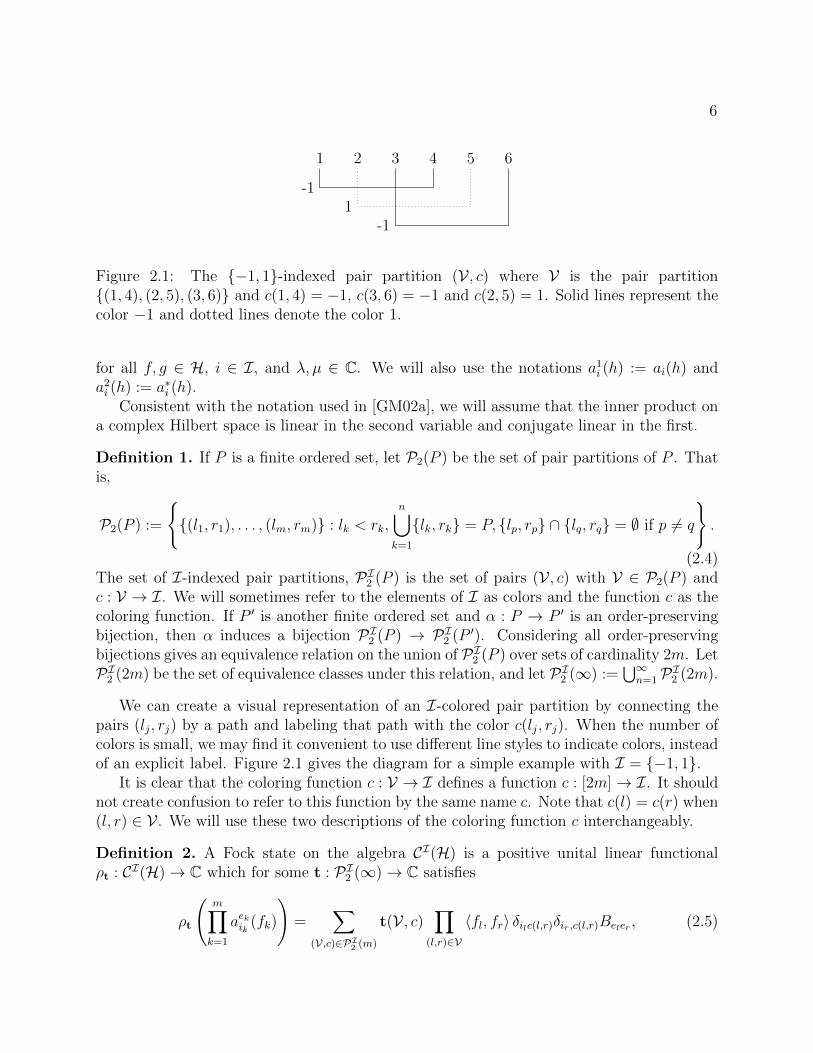
Figure 2.1: The −1, 1-indexed pair partition (V , c) where V is the pair partition(1, 4), (2, 5), (3, 6) and c(1, 4) = −1, c(3, 6) = −1 and c(2, 5) = 1. Solid lines represent thecolor −1 and dotted lines denote the color 1.

for all f, g ∈ H, i ∈ I, and λ, µ ∈ C. We will also use the notations a1i (h) := ai(h) and

a2i (h) := a∗i (h).

Consistent with the notation used in [GM02a], we will assume that the inner product ona complex Hilbert space is linear in the second variable and conjugate linear in the first.

Definition 1. If P is a finite ordered set, let P2(P ) be the set of pair partitions of P . Thatis,

P2(P ) :=

(l1, r1), . . . , (lm, rm) : lk < rk,

n⋃k=1

lk, rk = P, lp, rp ∩ lq, rq = ∅ if p 6= q

.

(2.4)The set of I-indexed pair partitions, PI2 (P ) is the set of pairs (V , c) with V ∈ P2(P ) andc : V → I. We will sometimes refer to the elements of I as colors and the function c as thecoloring function. If P ′ is another finite ordered set and α : P → P ′ is an order-preservingbijection, then α induces a bijection PI2 (P ) → PI2 (P ′). Considering all order-preservingbijections gives an equivalence relation on the union of PI2 (P ) over sets of cardinality 2m. LetPI2 (2m) be the set of equivalence classes under this relation, and let PI2 (∞) :=

⋃∞n=1PI2 (2m).

We can create a visual representation of an I-colored pair partition by connecting thepairs (lj, rj) by a path and labeling that path with the color c(lj, rj). When the number ofcolors is small, we may find it convenient to use different line styles to indicate colors, insteadof an explicit label. Figure 2.1 gives the diagram for a simple example with I = −1, 1.

It is clear that the coloring function c : V → I defines a function c : [2m]→ I. It shouldnot create confusion to refer to this function by the same name c. Note that c(l) = c(r) when(l, r) ∈ V . We will use these two descriptions of the coloring function c interchangeably.

Definition 2. A Fock state on the algebra CI(H) is a positive unital linear functionalρt : CI(H)→ C which for some t : PI2 (∞)→ C satisfies

ρt

(m∏k=1

aekik (fk)

)=

∑(V,c)∈PI2 (m)

t(V , c)∏

(l,r)∈V

〈fl, fr〉 δilc(l,r)δir,c(l,r)Beler , (2.5)

7

where for k ∈ [m], fk ∈ H the ek are chosen from 1, 2 and ik ∈ I.

B :=

(0 10 0

). (2.6)

Definition 3. A Gaussian state onAI(K) is a positive unital linear function ρt : AI(H)→ Cwhich for some t : PI2 (∞)→ C satisfies

ρt

(m∏k=1

ωik(fk)

)=

∑(V,c)∈PI2 (m)

t(V , c)∏

(l,r)∈V

〈fl, fr〉 δil,c(l,r)δir,c(l,r), (2.7)

any fk ∈ H (k ∈ [m]) and ik ∈ I.

Remark 1. If K is a real Hilbert space, then there is a canonical injection AI(K)→ CI(KC)given by

ωi(h) 7→ ai(h) + a∗i (h), (2.8)

where KC denotes the complexification of K. Considering CI(KC) as a subalgebra of AI(K),the restriction of a Fock state ρt on CI(KC) to AI(K) is a Gaussian state.

While we can use (2.7) and (2.5) to define linear functionals ρt and ρt for any choice oft : PI2 (∞)→ C, these linear functionals are not always positive. This leads to the followingdefinition.

Definition 4. A function t : PI2 (∞) → C is positive definite if ρt is a positive linearfunctional on CI(K) for any complex Hilbert space K.

Remark 2. Our definition of a positive definite function t : PI2 (∞) → C is modeled afterthe definition made for a single process in [GM02a] and is not obviously the same as thedefinition in [Gut03]. However, we will see in Theorem 3 that the definitions are equivalent.

Suppose that for each n : I → N ∪ 0, Vn is a complex Hilbert space with unitaryrepresentation Un of the direct product group

Sn :=∏b∈I

Sn(b), (2.9)

If H is a complex Hilbert space, then the Fock-like space is given by

FV (H) :=⊕n

1

n!Vn ⊗s H⊗n. (2.10)

Here H⊗n meansH⊗n :=

⊗b∈I

H⊗n(b), (2.11)

8

and n! means∏

b∈I n(b)!, and the factor 1n!

modifies the inner product. Also, we set H⊗0 =CΩ for some distinguished unit vector Ω. The notation ⊗s denotes the subspace of vectorswhich are invariant under the action of Sn given by Un⊗ Un, where Un is the natural actionof Sn on H⊗n. That is, Un(π) permutes the vectors according to π. The projection onto thesubspace 1

n!Vn ⊗s H⊗n is given by

Pn :=1

n!

∑σ∈Sn

U(σ)⊗ U(σ). (2.12)

For v ∈ Vn and f ∈ Hn we denote by v ⊗s f the vector Pn(v ⊗ f)To define creation and annihilation operators on the Fock-like space, we will also require

densely defined operators jb : Vn → Vn+δb (where δb(b′) = δb,b′) satisfying the following

intertwining relations:jbUn(σ) = Un+δb(ι

(b)n (σ))jb, (2.13)

where ι(b)n is the natural embedding of Sn into Sn+δb . Note that we have used the same

notation for the maps Vn → Vn+δb for different n, but the choice of n should be clear fromcontext so confusion should not result. We will call the maps jb the transition maps for ourHilbert spaces Vn.

Given transition maps, we can define creation and annihilation operators on the Fock-like

space FV (H) for each b ∈ I and each h ∈ H. Let(r

(n)b

)∗(h) be the operator(

r(n)b

)∗(h) : H⊗n → H⊗n+δb (2.14)

which acts as right creation operator on H⊗n(b) and identity on H⊗n(b′) for b′ 6= b. Let r(n)b (h)

be the adjoint of(r

(n)b

)∗(h). If n(b) 6= 0, then the annihilation operator aV,jb (f) is defined

on the level n component of the Fock-like space by

aV,jb (f) : Vn ⊗s H⊗n → Vn−δb ⊗s H⊗(n−δb)

aV,jb (f) : v ⊗s⊗b∈I

h(b)1 ⊗ · · · ⊗ h

(b)n(b)

7→n(b)∑k=1

〈f, hk〉n(b)

j∗b v ⊗s⊗

b′∈I\b

(h

(b′)1 ⊗ · · · ⊗ h(b′)

n(b′)

)⊗ h(b)

1 ⊗ · · · ⊗ h(b)k ⊗ · · · ⊗ h

(b)n(b)

.

(2.15)

If n(b) 6= 0, then aV,jb (f) (Vn ⊗s H⊗n) = 0.The creation operator (aV,jb )∗(h) is the adjoint of aV,jb (h), and its action on a vector v⊗s f

is given by(aV,jb )∗(h) (vn ⊗s f) = (n(b) + 1)(jbvn)⊗s (rnb )∗ (h)f . (2.16)

9

We denote by CV,j(H) the ∗-algebra generated by the operators aV,jb (f) and (aV,jb )∗(f) forf ∈ H, and b ∈ I.

There is a representation νV,j of CI(H) on the Fock-like space FV (H) satisfying

νV,j : ab(f) 7→ aV,jb (f) and a∗b(f) 7→ (aV,jb )∗(f) (2.17)

for all b ∈ I and f ∈ H. We will usually identify X ∈ CI(H) with its image νV,j(X).We will sometimes write ab(f) and a∗b(f) for the annihilation and creation operators

aV,jb (f) and(aV,jb

)∗(f). We will also use the notation aV,j,1b (f) or simply a1

b(f) for aV,jb (f)

and likewise aV,j,2b (f) or simply a2b(f) for (aV,jb )∗(f).

The following is an I-indexed generalization of Theorem 2.6 of [GM02a].

Theorem 1. Let I be an index set and H a complex Hilbert space. Let (Un, Vn) be repre-sentations of Sn with maps jb : Vn → Vn+δb satisfying the intertwining relation (2.13). LetξV ∈ V0 be a unit vector. The state ρV,j on CI(H) defined by

ρV,j(X) = 〈ξV ⊗s Ω, X(ξV ⊗s Ω)〉 (2.18)

is a Fock state. That is, there is a positive definite function t such that ρV,j = ρt.

The proof is very similar to the proof of Theorem 2.6 of [GM02a], but we include it forcompleteness.

Proof. Let H be an infinite-dimensional complex Hilbert space, and let fk∞k=1 be an or-thonormal basis for H. Also let V = (lk, rk) : k ∈ [n] with lk < rk for 1 ≤ k ≤ n andlk < lk′ for k < k′.

Define

t((V , c)) = ρV,j

(n∏k=1

aekbk (fk)

)

=

⟨ξV ⊗s Ω,

(n∏k=1

aekbk (fk)

)(ξV ⊗s Ω)

⟩ (2.19)

where bk and ek are chosen as follows. Each k is an element of one pair (li, ri) ∈ V for somei. If k = li, we let ek = 1, and if k = ri we let ek = 2. In either case, we let bk = c(li, ri).

For A ∈ B(H) and b ∈ I, define the operator dΓbV (A) on FV (H) by

dΓbV (A) :v ⊗s⊗b′∈I

hb′,1 ⊗ · · · ⊗ hb′,m′b 7→

mb∑k=1

v ⊗s

(⊗b′ 6=b

hb′,1 ⊗ · · · ⊗ hb′,mb′

)⊗ (hb,1 ⊗ · · · ⊗ Ahb,k ⊗ · · · ⊗ hb,mb) .

(2.20)

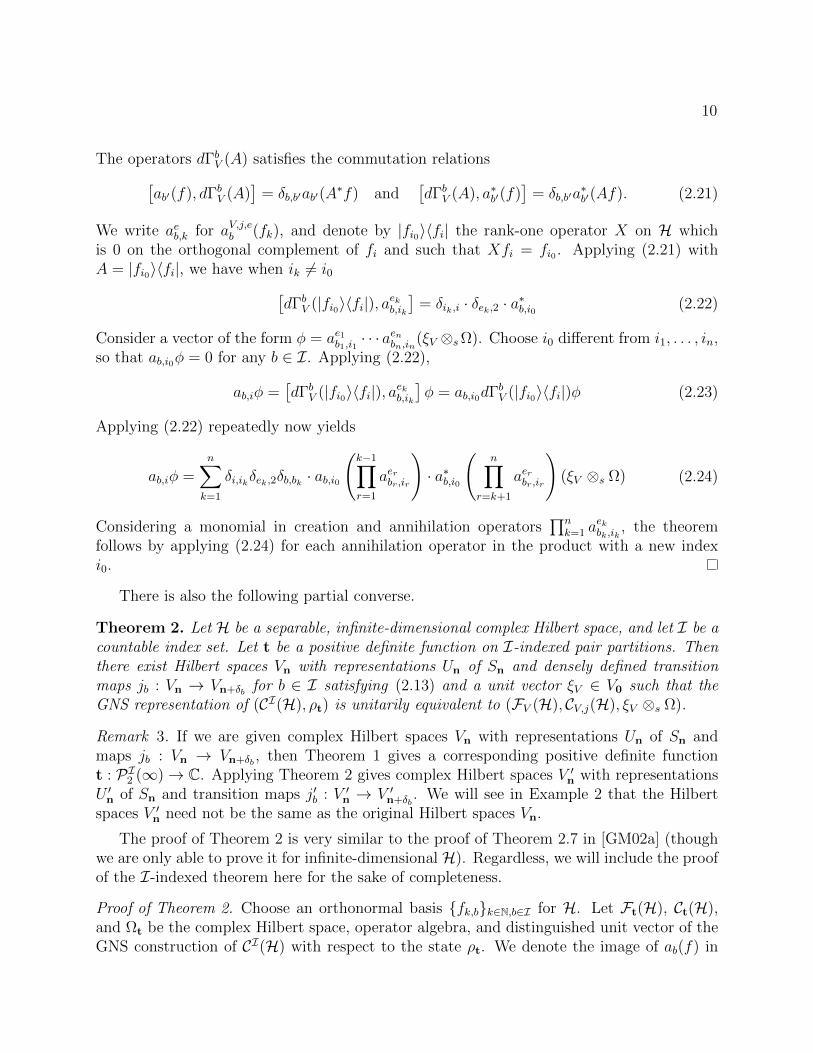
10

The operators dΓbV (A) satisfies the commutation relations[ab′(f), dΓbV (A)

]= δb,b′ab′(A

∗f) and[dΓbV (A), a∗b′(f)

]= δb,b′a

∗b′(Af). (2.21)

We write aeb,k for aV,j,eb (fk), and denote by |fi0〉〈fi| the rank-one operator X on H whichis 0 on the orthogonal complement of fi and such that Xfi = fi0 . Applying (2.21) withA = |fi0〉〈fi|, we have when ik 6= i0[

dΓbV (|fi0〉〈fi|), aekb,ik

]= δik,i · δek,2 · a∗b,i0 (2.22)

Consider a vector of the form φ = ae1b1,i1 · · · aenbn,in

(ξV ⊗sΩ). Choose i0 different from i1, . . . , in,so that ab,i0φ = 0 for any b ∈ I. Applying (2.22),

ab,iφ =[dΓbV (|fi0〉〈fi|), a

ekb,ik

]φ = ab,i0dΓbV (|fi0〉〈fi|)φ (2.23)

Applying (2.22) repeatedly now yields

ab,iφ =n∑k=1

δi,ikδek,2δb,bk · ab,i0

(k−1∏r=1

aerbr,ir

)· a∗b,i0

(n∏

r=k+1

aerbr,ir

)(ξV ⊗s Ω) (2.24)

Considering a monomial in creation and annihilation operators∏n

k=1 aekbk,ik

, the theoremfollows by applying (2.24) for each annihilation operator in the product with a new indexi0.

There is also the following partial converse.

Theorem 2. Let H be a separable, infinite-dimensional complex Hilbert space, and let I be acountable index set. Let t be a positive definite function on I-indexed pair partitions. Thenthere exist Hilbert spaces Vn with representations Un of Sn and densely defined transitionmaps jb : Vn → Vn+δb for b ∈ I satisfying (2.13) and a unit vector ξV ∈ V0 such that theGNS representation of (CI(H), ρt) is unitarily equivalent to (FV (H), CV,j(H), ξV ⊗s Ω).

Remark 3. If we are given complex Hilbert spaces Vn with representations Un of Sn andmaps jb : Vn → Vn+δb , then Theorem 1 gives a corresponding positive definite functiont : PI2 (∞)→ C. Applying Theorem 2 gives complex Hilbert spaces V ′n with representationsU ′n of Sn and transition maps j′b : V ′n → V ′n+δb

. We will see in Example 2 that the Hilbertspaces V ′n need not be the same as the original Hilbert spaces Vn.

The proof of Theorem 2 is very similar to the proof of Theorem 2.7 in [GM02a] (thoughwe are only able to prove it for infinite-dimensional H). Regardless, we will include the proofof the I-indexed theorem here for the sake of completeness.

Proof of Theorem 2. Choose an orthonormal basis fk,bk∈N,b∈I for H. Let Ft(H), Ct(H),and Ωt be the complex Hilbert space, operator algebra, and distinguished unit vector of theGNS construction of CI(H) with respect to the state ρt. We denote the image of ab(f) in

11

Ct(H) by atb(f) and the image of a∗b(f) in Ct(H) by (atb)∗(f). We will use the notation at,eb (f)

to mean (at)∗b (f) for e = 2 and atb(f) for e = 1. We will construct the complex Hilbert

spaces Vn as subspaces of Ft(H).Suppose that for each function n : I → N∪0 which is 0 at all but finitely many points

in I and each i ∈ I, we have an injective function αn,i : [n(i)]→ N and that αn,i(j) = αn′,i(j)when j < n(i),n′(i).

Denote by Rαn the set of the vectors of the form

at,e1b1(fb1,i1) · · · a

t,e2p+|n|b2p+|n|

(fb2p+|n|,i2p+|n|)Ωt, (2.25)

where |n| =∑

b∈I n(b) satisfying the following conditions:

1. In the product at,e1b1(fb1,i1) · · · a

t,e2p+|n|b2p+|n|

(fb2p+|n|,i2p+|n|), a creation operator at,2b (fb,αb(j))

appears exactly once provided that 1 ≤ j ≤ n(b).

2. Among the remaining 2p operators in the product, there are p creation operators(at,2bq (fbq ,lq))

pq=1 and p annihilation operators (at,1bq (fbq ,lq))

pq=1. Moreover, each annihila-

tion operator appears to the left of the corresponding creation operator in the product.

We also let V αn be the span of the vectors in Rα

n. We define the map jαb′ : V αn → V α

n+δb′by

restricting the creation operator at,2b′ (fb′,αn,b′ (n(b′))) to the subspace V αn of Ft(H). It follows

immediately from the definition of V αn that the image of this restriction lies in V α

n+δb′.

We define a unitary representation Uαn of Sn on V α

n . Since ρt is a Fock state, it is invariantunder unitary transformations U on H in the sense that

ρt

(n∏k=1

aekbk (fbk,ik)

)= ρt

(n∏k=1

aekbk (Ufbk,ik)

). (2.26)

Therefore, there is a unitary map Ft(U) given by

Ft(U) :n∏k=1

at,ekbk(fbk,ik)Ωt 7→

n∏k=1

aekbk (Ufbk,ik)Ωt. (2.27)

The map Ft(U) induces an automorphism on the algebra of creation and annihilation oper-ators by

Ft(U)at,ekbk(h)Ft(U

∗) = at,ekbk(Uh). (2.28)

For σ ∈ Sn, let Uασ be the unitary operator on H which for each b ∈ I acts by permuting

fb,αn,b(1), . . . , fb,αn,b(n(b)) according to σ and fixes fb,r when r > n(b). The map Uαn : σ 7→ Uα

σ

is a unitary representation of Sn on V αn .

Define ιn,i : [n(i)] → N by ιn,i(j) = j, and let Rn := Rιn, Vn := V ι

n, jb := jιb, and letUn := Uα

n . It follows from the definitions that these data satisfy the intertwining property(2.13). We also define ξV := Ωt ∈ V0.

12

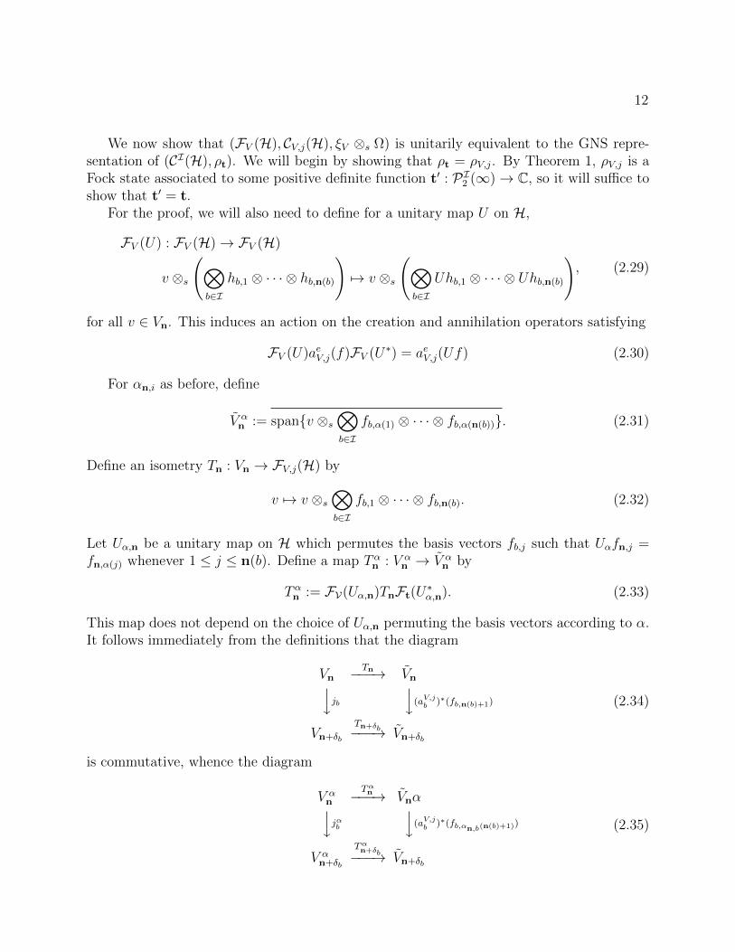
We now show that (FV (H), CV,j(H), ξV ⊗s Ω) is unitarily equivalent to the GNS repre-sentation of (CI(H), ρt). We will begin by showing that ρt = ρV,j. By Theorem 1, ρV,j is aFock state associated to some positive definite function t′ : PI2 (∞)→ C, so it will suffice toshow that t′ = t.

For the proof, we will also need to define for a unitary map U on H,

FV (U) : FV (H)→ FV (H)

v ⊗s

(⊗b∈I

hb,1 ⊗ · · · ⊗ hb,n(b)

)7→ v ⊗s

(⊗b∈I

Uhb,1 ⊗ · · · ⊗ Uhb,n(b)

), (2.29)

for all v ∈ Vn. This induces an action on the creation and annihilation operators satisfying

FV (U)aeV,j(f)FV (U∗) = aeV,j(Uf) (2.30)

For αn,i as before, define

V αn := spanv ⊗s

⊗b∈I

fb,α(1) ⊗ · · · ⊗ fb,α(n(b)). (2.31)

Define an isometry Tn : Vn → FV,j(H) by

v 7→ v ⊗s⊗b∈I

fb,1 ⊗ · · · ⊗ fb,n(b). (2.32)

Let Uα,n be a unitary map on H which permutes the basis vectors fb,j such that Uαfn,j =fn,α(j) whenever 1 ≤ j ≤ n(b). Define a map Tαn : V α

n → V αn by

Tαn := FV(Uα,n)TnFt(U∗α,n). (2.33)

This map does not depend on the choice of Uα,n permuting the basis vectors according to α.It follows immediately from the definitions that the diagram

VnTn−−−→ Vnyjb y(aV,jb )∗(fb,n(b)+1)

Vn+δb

Tn+δb−−−→ Vn+δb

(2.34)

is commutative, whence the diagram

V αn

Tαn−−−→ Vnαyjαb y(aV,jb )∗(fb,αn,b(n(b)+1))

V αn+δb

Tαn+δb−−−→ Vn+δb

(2.35)

13

also commutes. A similar argument gives a corresponding commutative diagram for theannihilation operators, and this implies the equality of the states ρt and ρV,j, which impliest = t.

Finally, we must prove that the vacuum vector ΩV := ξV ⊗ Ω is cyclic for CI(H). It willsuffice to show that for any n, any v ∈ Rn and any vectors h1, . . . , hn ∈ H, there is someX ∈ CI(H) with

XΩV = v ⊗s⊗b∈I

hb,1 ⊗ · · · ⊗ hb,n(b). (2.36)

By the definition of Rn, we can write

v =

2p+|n|∏k=1

at,ekbk(fbk,ik)

Ωt (2.37)

where a creation operator at,2b (fb,j) appears exactly once for 1 ≤ j ≤ n(b), and among theremaining 2p operators in the product, there are p creation operators (at,2bq (fbq ,lq))

pq=1 and p

annihilation operators at,1bq (fbq ,lq)pq=1, with each annihilation operator appearing to the left of

the corresponding creation operator in the product. We need simply choose X of the form

X :=1

n!·

2p+|n|∏k=1

aekbk (gk), (2.38)

where the gk satisfy:

gk :=

hbk,rk , if 1 ≤ ik ≤ n(bk)

h′lk , otherwise, (2.39)

where rk is defined so that k is the rk-th smallest element of the set u : bu = bk, 1 ≤ u ≤n(bk), the (h′i)

∞i=1 are an orthonormal sequence of vectors which are orthogonal to each hb,k,

and lk = l′k if and only if bk = bk′ and ik = ik′ . It follows from the definitions that this Xsatisfies (2.36), so the proof is complete.

We now pursue an algebraic characterization of positive definiteness for functions onI-indexed pair partitions. This will involve Guta’s ∗-semigroup of I-indexed broken pairpartitions [Gut03].

Definition 5. Let X be an arbitrary finite ordered set and (La, Pa, Ra)a∈I a disjoint partitionof X into triples of subsets indexed by elements of I. Suppose that for each a ∈ I, we havea triple (Va, f (l)

a , f(r)a ) where Va ∈ P2(Pa) and

f (l)a : La → 1, . . . , |La| and f (r)

a : Ra → 1, . . . , |Ra| (2.40)

are bijective. An order preserving bijection α : X → Y induces a map

αa : (Va, f (l)a , f (r)

a )→ (α Va, f (l)a α−1, f (r)

a α−1) (2.41)

14

1

2

2

1

3

1

4

1

d =

1 42

1

3 65

1

d =

Figure 2.2: The diagram of the −1, 1-colored broken pair partitions d and d. Here d =

Va, f (l)a , f

(r)a a∈−1,1 and d = Va, f (l)

a , f(r)a a∈−1,1, with the following definitions. For d,

V−1 = V1 is the unique pair partition on the empty set and the right and left leg functions are

defined by f(l)−1 : ∅ → ∅,f (l)

1 : 2 → 1 given by f(l)1 (2) = 1, f

(r)−1 : 1, 3 → 1, 2 given by

f(r)−1 (1) = 2 and f

(r)−1 (3) = 1, and f

(r)1 : 4 → 1 given by f

(r)1 (4) = 1. For d, V2 = (1, 4),

V1 = (3, 6) and the right and left leg functions are defined by f(l)−1 : 2 → 1 with

f(l)−1(2) = 1, f

(l)1 : ∅ → ∅, f (r)

1 : ∅ → ∅, and f(r)1 : 5 → 1 given by f

(r)1 (5) = 1. The solid

lines represent the “color” −1 and the dotted lines represent the “color” 1.

where α V := (α(i), α(j)) : (i, j) ∈ V. This determines an equivalence relation on the setof such I-indexed triples, and we call an equivalence class under this relation an I-indexedbroken pair partition. We denote the set of all I-indexed broken pair partition by BPI2 (∞).

There is a convenient diagrammatic representation of a broken pair partition. Given abroken pair partition as just defined, we write the elements of the base set X in order. Foreach pair (x, x′) ∈ Va, we connect x and x′ by a piecewise-linear path and label that pathwith the index a. For each index a ∈ I such that La 6= ∅, we write the numbers 1, . . . , |La|in order on the left side and connect each y ∈ La to the number f

(l)a (y). Likewise, for each

color a ∈ I such that Ra 6= ∅, we write the numbers 1, . . . , |Ra| in order on the left side and

connect each y ∈ Ra to the number f(l)a (y). When |I| is small, we may also use different line

styles (e.g. dotted and solid lines) to indicate the different colors a ∈ I. Figure 2.2 givestwo examples of these diagrams.

The diagrammatic representations of the I-colored broken pair partitions inspires someadditional terminology. Namely, we call the functions f

(l)a and f

(r)a the left and right leg

functions for the color a. Moreover, we call the piecewise-linear paths from the domains off

(l)a and f

(r)a to the numbers f

(l)a (y) and f

(r)a (y) the left and right legs of the I-colored broken

pair partitions. This terminology will be useful in describing the semigroup structure onBPI2 (∞).

In the case that |I| = 1, we recover the (uncolored) broken pair partitions of Guta andMaassen [GM02a]. Moreover, each d ∈ BPI2 (∞) gives for each a ∈ I a broken pair partitionda in the sense of [GM02a]. However, all but finitely many of the da are the unique brokenpair partition on the empty set.

The space BPI2 (∞) can be given the structure of a semigroup with involution, similar tothe ∗-semigroup of broken pair partitions of [GM02a]. In terms of the diagrams, multiplica-tion of two I-colored broken pair partitions corresponds to concatenation of diagrams. Right

15

legs of the first diagram are joined with left legs of the second diagram of the same color toform pairs. In the event that the second diagram has more left legs of some color a than thefirst diagram has right legs of color a, we join the right legs of the first diagram with thelargest-numbered left legs of the second diagram, and the remaining left legs of the seconddiagram are extended to become low-numbered left legs in the product. An analogous ruleis used when the first diagram has more right legs of some color a than the second diagramhas left legs of color a.

The precise definition of the product on BPI2 (∞) is as follows. For i = 1, 2, let di =

(Va,i, f (l)a,i , f

(r)a,i )a∈I be an I-colored broken pair partition on the ordered base set Xi. The

product is a broken pair partition on the base setX := X1

∐X2 with the order relation x < x′

if either x < x′ in Xi or x ∈ X1 and x ∈ X2. For each a ∈ I, define Ma = min(|Ra,1|, |La,2|).Following [Gut03], we define

d1 · d2 = (Va, f (l)a , f (r)

a )a∈I , (2.42)

where

Va = Va,1 ∪ Va,2 ∪(

(f(r)a,1)−1([|Ra,1| − j]), (f (l)

a,2)−1([|La,2| − j]))

: j ∈ [Ma]

(2.43)

and f(l)a is defined on the disjoint union of La,1 and (f

(l)a,2)−1([|La,2| −Ma]) by

f (l)a (i) =

f

(l)a,1(i), if i ∈ La,1f

(l)a,2(i) + |La,1| −Ma, if i ∈ (f

(l)a,2)−1([|La,2| −Ma])

. (2.44)

The function of right legs, f(r)a is defined on the disjoint union of Ra,2 and (f

(r)a,1)−1([|Ra,1| −

Ma]) by

f (r)a (i) =

f

(r)a,2(i), if i ∈ Ra,2

f(r)a,1(i) + |Ra,2| −Ma, if i ∈ (f

(r)a,1)−1([|Ra,1| −Ma])

. (2.45)

An example of multiplication of I-colored broken pair partitions is illustrated in Figure 2.3.1

The involution is given by mirror reflection of the I-colored broken pair partitions. For-mally, if d = (Va, f (l)

a , f(r)a )a∈I with underlying set X then d∗ = (V∗a , f

(r)a , f

(l)a )a∈I is an

I-colored broken pair partition with underlying set X∗, the same as X but with the orderreversed, where V∗a = (i, j) : (j, i) ∈ Va. The involution is illustrated in Figure 2.4.

For each function n : I → N which is zero except on finitely many elements of I, letBPI2 (n,0) be the subset of BPI2 (∞) consisting of elements having exactly n(a) left legs ofcolor a and no right legs.

1The multiplication for BPI2 (∞) stated here differs slightly from that stated in [Gut03]. We believe that

the rule stated here is the one intended by the author of that work, as it ensures that condition (2.13) issatisfied. However, we do not believe that this discrepancy is consequential for Guta’s results.

16

1

2

2

1

3

1

4

1

·1 42

1

3 65

1

=1 62

1

3

1

4

2

5 87 109

1

Figure 2.3: The multiplication d · d of the −1, 1-colored broken pair partitions defined inFigure 2.2.

63 5

1

41 2

1

d∗ =

Figure 2.4: The involution of the −1, 1-colored broken pair partition d depicted in Figure2.1.

1 52 83 64 107 9

Figure 2.5: The standard form of the pair partition (V , c) ∈ PI2 (10) with I = −1, 1and V = (1, 5), (2, 8), (3, 6), (4, 10), (7, 9) and c((1, 5)) = c((2, 8)) = c((7, 9)) = −1 andc((3, 6)) = c((4, 10)) = 1. The solid lines represent the “color” −1 and the dotted linesrepresent the “color” 1.

Let da be the unique element of BPI2 (∞) with no right legs, no pairs, and only one leftleg, colored a ∈ I. We call da the a-colored left hook and d∗a the a-colored right hook.

An I-colored broken-pair partition can be written as a sequence of left hooks, followed bypermutations acting on the legs of the same color, followed by right hooks connecting with leftlegs of the same index, possibly followed by additional sequences of left hooks, permutations,and right hooks. The “standard form” of an element of PI2 (∞) is the sequence of this formsuch that if two like-colored pairs cross, they do so in the rightmost permutation possible.Figure 2.5 depicts the standard form of one example.

As in [Gut03], we can use the standard form of (V , c) for V ∈ P2(2m) to compute thevalue of t((V , c)) as follows. Consider c as a function [2m] → I taking the same value on

points belonging to the same pair of V . Partition [2m] into 2t blocks B(r)i , B

(l)i for i = 1, . . . , t

such that the B(l)i contain left legs of the pairs of V and the B

(r)i contain right legs of the

17

pairs of V . Write B(r)i := ki−1, . . . , pi and B

(l)j := pi+1, . . . , ki with k0 = 1 and kr = 2m.

Then there are permutations πj such that

(V , c) =

p1∏l=1

d∗c(l)Un1(π1)

k1∏l=p1+1

dc(l) · · ·Unr(πr)2m∏

l=pt+1

dc(l) (2.46)

The function on pair partitions can then be calculated as

tV,j((V , c)) =

⟨ξV ,

p1∏l=1

j∗c(l)Un1(π1)

k1∏l=p1+1

jc(l) · · ·Unr(πr)2m∏

l=pt+1

jc(l)ξV

⟩. (2.47)

An I-colored pair partition V can be considered as an element of BPI2 (∞) having noleft or right legs in the obvious way. A function t : PI2 (∞)→ C thus extends to a functiont : BPI2 (∞)→ C by

t(d) =

t(d), if d ∈ PI2 (∞),

0, otherwise. (2.48)

The following is an I-indexed generalization of Theorem 3.2 of [GM02a].

Theorem 3. A function t : PI2 (∞) → C is positive definite if t : BPI2 (∞) → C is posi-tive definite in the usual sense of positive definiteness for a function on a semigroup withinvolution.

The proof is very similar to the proof of Theorem 3.2 of [GM02a], but we include it forcompleteness.

Proof. Suppose that t is positive definite on the ∗-semigroup BPI2 (∞). Then there is arepresentation χ of BPI2 (∞) on a complex Hilbert space V having cyclic vector ξ ∈ V suchthat

〈ξ, χ(d)ξ〉 = t(d) (2.49)

for all d ∈ BPI2 (∞).The complex Hilbert space V is expressible as a direct sum

V =⊕n

Vn, (2.50)

where the sum is over functions n : I → N with only finitely many nonzero values and

Vn = spanχt(d)ξ : d ∈ BPI2 (n,0). (2.51)

The action of Sn on BPI2 (n,0) (by permutation of the left legs) gives a unitary representationUn of Sn on Vn. Restriction of jb := χ(db) (where, as before db is the b-colored left hook)gives a map jb : Vn → Vn+δb satisfying (2.13). Choose a unit vector ξV ∈ V0.

18

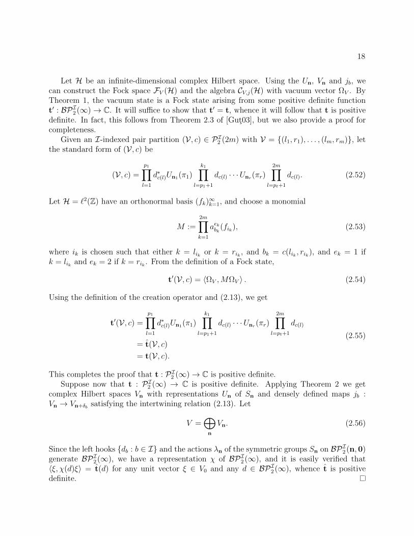
Let H be an infinite-dimensional complex Hilbert space. Using the Un, Vn and jb, wecan construct the Fock space FV (H) and the algebra CV,j(H) with vacuum vector ΩV . ByTheorem 1, the vacuum state is a Fock state arising from some positive definite functiont′ : BPI2 (∞)→ C. It will suffice to show that t′ = t, whence it will follow that t is positivedefinite. In fact, this follows from Theorem 2.3 of [Gut03], but we also provide a proof forcompleteness.

Given an I-indexed pair partition (V , c) ∈ PI2 (2m) with V = (l1, r1), . . . , (lm, rm), letthe standard form of (V , c) be

(V , c) =

p1∏l=1

d∗c(l)Un1(π1)

k1∏l=p1+1

dc(l) · · ·Unr(πr)2m∏

l=pt+1

dc(l). (2.52)

Let H = `2(Z) have an orthonormal basis (fk)∞k=1, and choose a monomial

M :=2m∏k=1

aekbk (fik), (2.53)

where ik is chosen such that either k = lik or k = rik , and bk = c(lik , rik), and ek = 1 ifk = lik and ek = 2 if k = rik . From the definition of a Fock state,

t′(V , c) = 〈ΩV ,MΩV 〉 . (2.54)

Using the definition of the creation operator and (2.13), we get

t′(V , c) =

p1∏l=1

d∗c(l)Un1(π1)

k1∏l=p1+1

dc(l) · · ·Unr(πr)2m∏

l=pt+1

dc(l)

= t(V , c)= t(V , c).

(2.55)

This completes the proof that t : PI2 (∞)→ C is positive definite.Suppose now that t : PI2 (∞) → C is positive definite. Applying Theorem 2 we get

complex Hilbert spaces Vn with representations Un of Sn and densely defined maps jb :Vn → Vn+δb satisfying the intertwining relation (2.13). Let

V =⊕n

Vn. (2.56)

Since the left hooks db : b ∈ I and the actions λn of the symmetric groups Sn on BPI2 (n,0)generate BPI2 (∞), we have a representation χ of BPI2 (∞), and it is easily verified that〈ξ, χ(d)ξ〉 = t(d) for any unit vector ξ ∈ V0 and any d ∈ BPI2 (∞), whence t is positivedefinite.

19

Guta [Gut03] considered the case in which the Vn and the ja are defined as follows.Let t : PI2 (∞) → C be a positive definite function. As before, denote by BPI2 (n,0) theset of d ∈ BPI2 (∞) having |Ra| = 0 and |La| = n(a) for each a ∈ I. Consider the GNSrepresentation (χt, V, ξt) of BPI2 (n,0) with respect to t, characterized by

〈χt(d1)ξt, χt(d2)ξt〉V = t(d∗1d2). (2.57)

The complex Hilbert space V is given by

V :=⊕n

Vn where Vn = spanχt(d)ξt : d ∈ BPI2 (n,0). (2.58)

Each Vn has a representation of Sn with Sn(a) acting by permuting the left legs of BPI2 (n,0)

of color a. That is for π = (πa)a∈I ∈ Sn and (Va, f (l)a , f

(r)a )a∈I ∈ BPI2 (n,0),

Un(π)(Va, f (l)a , f (r)

a )a∈I = (Va, π−1a f (l)

a , f (r)a )a∈I . (2.59)

We denote by Ft(H) the Fock-like space arising from using these Vn in (2.10)

Ft(H) :=⊕n

1

n!Vn ⊗s

⊗H⊗n. (2.60)

The creation and annihilation operators on Ft(H) will be assumed to be those associatedto the following operators ja. For a ∈ I, denote by ja the operator χt(da), where da is thebroken pair partition with no pairs, no right legs, and one a-colored left leg.

We can now state the following theorem of Guta [Gut03].

Theorem 4. Let f1, . . . , fn be vectors in a complex Hilbert space H. Then the expectationvalues with respect to the vacuum state ρt of the monomials in creation and annihilationoperators on the Fock space Ft(H) have the expression

ρt

(m∏i=1

aeibi(fi)

)=

∑(V,c)∈PI2 (n)

t(V , c)∏

(i,j)∈V

〈fi, fj〉 δbi,bjBeiej , (2.61)

where the ei are chosen from 1, 2 and

B :=

(0 10 0

). (2.62)

20

Chapter 3

Factor representations of S∞

In Chapter 4, we will take an interest in noncommutative generalized Brownian motionswhich are related to factor representations of the group S∞ of permutations of N which fixall but finitely many points. Here we briefly recall some relevant background informationpertaining to those representations.

The finite factor representations of a group are determined by the group’s characters,that is, the positive, normalized indecomposable functions which are constant on conjugacyclasses. In the case of S∞, the characters are given by the following famous result.

Theorem 5 (Thoma’s Theorem [Tho64]). The normalized finite characters of S∞ are givenby the formula

φα,β(σ) =∏m≥2

(∞∑i=1

αmi + (−1)m+1

∞∑i=1

βmi

)ρm(σ)

(3.1)

where ρm(σ) is the number of cycles of length m in the permutation σ, and (αi)∞i=1 and (βi)

∞i=1

are decreasing sequences of positive real numbers such that∑

i αi +∑

i βi ≤ 1.

The pairs of sequences (αi)∞i=1 and (βi)

∞i=1 satisfying the conditions in Theorem 5 are

commonly called Thoma parameters.We now recall Vershik and Kerov’s representation of the symmetric group Sn (for n ∈

0, 1, 2, . . . ,∞) [VK82].

Notation 4. Fix sequences (αi)∞i=1 and (βi)

∞i=1, and let γ = 1−

∑i αi−

∑i βi and let N+ and

N− be two copies of the set N = 1, 2, . . .. Let Q := N+∪N−∪[0, γ], and define a measure µon Q to be the Lebesgue measure on [0, γ] and such that µ(i) = αi for i ∈ N+ and µ(j) = βjfor j ∈ N−. Let Xn denote the n-fold Cartesian product of Q with the product measuremn =

∏n1 µ, and let Sn act on Xn by σ(x1, . . . , xn) = (xσ−1(1), . . . , xσ−1(n)). For x, y ∈ Xn,

say that x ∼ y if there exists σ ∈ Sn such that x = σy. Let Xn = (x, y) ∈ Xn×Xn : x ∼ y.

21

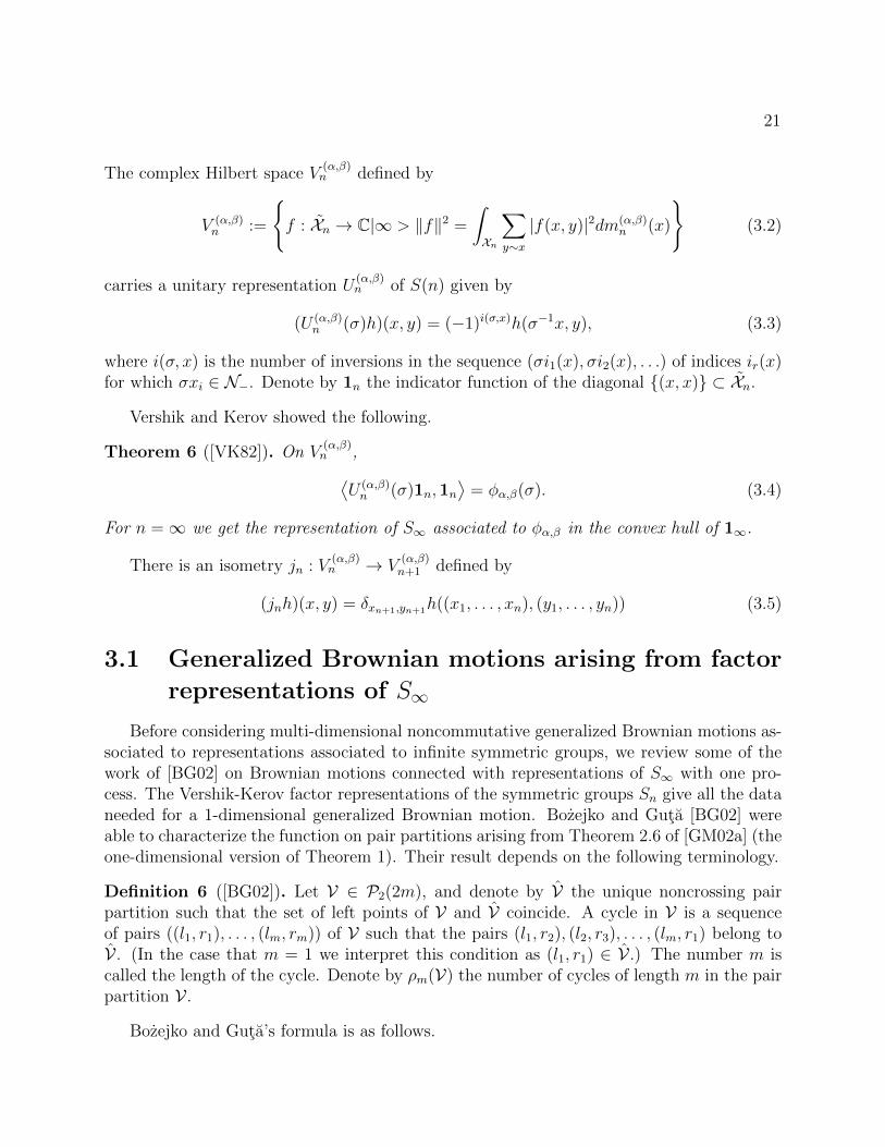
The complex Hilbert space V(α,β)n defined by

V (α,β)n :=

f : Xn → C|∞ > ‖f‖2 =

∫Xn

∑y∼x

|f(x, y)|2dm(α,β)n (x)

(3.2)

carries a unitary representation U(α,β)n of S(n) given by

(U (α,β)n (σ)h)(x, y) = (−1)i(σ,x)h(σ−1x, y), (3.3)

where i(σ, x) is the number of inversions in the sequence (σi1(x), σi2(x), . . .) of indices ir(x)for which σxi ∈ N−. Denote by 1n the indicator function of the diagonal (x, x) ⊂ Xn.

Vershik and Kerov showed the following.

Theorem 6 ([VK82]). On V(α,β)n ,⟨

U (α,β)n (σ)1n,1n

⟩= φα,β(σ). (3.4)

For n =∞ we get the representation of S∞ associated to φα,β in the convex hull of 1∞.

There is an isometry jn : V(α,β)n → V

(α,β)n+1 defined by

(jnh)(x, y) = δxn+1,yn+1h((x1, . . . , xn), (y1, . . . , yn)) (3.5)

3.1 Generalized Brownian motions arising from factor

representations of S∞

Before considering multi-dimensional noncommutative generalized Brownian motions as-sociated to representations associated to infinite symmetric groups, we review some of thework of [BG02] on Brownian motions connected with representations of S∞ with one pro-cess. The Vershik-Kerov factor representations of the symmetric groups Sn give all the dataneeded for a 1-dimensional generalized Brownian motion. Bozejko and Guta [BG02] wereable to characterize the function on pair partitions arising from Theorem 2.6 of [GM02a] (theone-dimensional version of Theorem 1). Their result depends on the following terminology.

Definition 6 ([BG02]). Let V ∈ P2(2m), and denote by V the unique noncrossing pairpartition such that the set of left points of V and V coincide. A cycle in V is a sequenceof pairs ((l1, r1), . . . , (lm, rm)) of V such that the pairs (l1, r2), (l2, r3), . . . , (lm, r1) belong toV . (In the case that m = 1 we interpret this condition as (l1, r1) ∈ V .) The number m iscalled the length of the cycle. Denote by ρm(V) the number of cycles of length m in the pairpartition V .

Bozejko and Guta’s formula is as follows.

22

Theorem 7 ([BG02]). Let (αi)∞i=1 and (βi)

∞i=1 be decreasing sequences of positive real numbers

such that∑

i αi +∑

i βi ≤ 1. Let V(α,β)n be the complex Hilbert space of the Vershik-Kerov

representation of Sn, and let jn : V(α,β)n → V

(α,β)n+1 be the natural isometry. Let ξV (α,β) = 10.

Denote by tα,β the function on P2(∞) associated to these representations by Theorem 1.Then

tα,β(V) =∏m≥2

(∞∑i=1

αmi + (−1)m+1

∞∑i=1

βmi

)ρm(V)

. (3.6)

Remark 4. There is another equivalent characterization of the cycle decomposition of apair partition. As in Definition 6, let V = (a1, z1), . . . , (an, zn) ∈ P2(2m) and let V bethe noncrossing pair partition whose left points coincide with those of V . Let σ ∈ Snbe the permutation such that V = (a1, zσ−1(1)), . . . , (an, zσ−1(n)). If the cycles of σ areτi = (bi1 · · · biri) ∈ Sn (1 ≤ i ≤ m), then the cycles of V are (abi1 , zbi1), . . . , (abiri , zbiri ).Moreover, Theorem 7 says that tα,β(V) = φα,β(σ).

We are now in a position to show that the framework for multi-dimensional generalizedBrownian motion presented here is more general than that presented in [Gut03]. Moreprecisely, we will exhibit complex Hilbert spaces Vn with representations Un of Sn andtransition maps jb : Vn → Vn+δb and V ′n with representations U ′n of Sn and maps jb : V ′n →V ′n+δb

such that both sets of data give rise to the same function on pair partitions accordingto Theorem 1.

Example 2. We work with the index set I = 1, which places us in the setting of thegeneralized Brownian motion with only one process, developed by Guta and Maassen in[GM02a]. Fix an integer N with |N | > 1 and let H be a complex Hilbert space. We willconsider generalized Brownian motions associated to the character φN of S∞ given by thesequences

αn =

1N, if 1 ≤ n ≤ N

0, otherwiseand βn =

1N, if 1 ≤ n ≤ −N

0, otherwise(3.7)

For each n, let V(N)n be the complex Hilbert space of the Vershik-Kerov representation of Sn,

and let j(N) : V(N)n → V

(N)n+1 be the natural isometry. Let ξV (N) = 10 be the indicator function

of the diagonal. Denote by tN the function on P2(∞) associated to these representations byTheorem 1. It was shown in [BG02] that

tN(V) =

(1

N

)n−ρ(V)

. (3.8)

We will exhibit another sequence of complex Hilbert spaces V(N)n with unitary represen-

tations U(N)n which gives rise to the same positive function on pair partitions. Since the

character φN : S∞ → C restricts to a positive definite function on Sn, there is a representa-tion U

(N)n of Sn on a complex Hilbert space V

(N)n with a cyclic vector ξn such that⟨

ξn, U(N)n (π)ξn

⟩= φN(π). (3.9)

23

for every π ∈ Sn. There is also a natural inclusion j(N) : V(N)n → V

(N)n+1 satisfying

j(U (N)n (π)ξn) = U

(N)n+1(ιnπ)ξn+1, (3.10)

where ιn is the inclusion Sn → Sn+1 induced by the natural inclusion [n] ⊂ [n+ 1]. By con-

struction, the maps j(N) and representations V(N)n satisfy the intertwining relation (2.13),

so we can construct the Fock space FV (N),j(N) with creation and annihilation operatorsa∗V (N),j(N)(f) and aV (N),j(N)(f).

The action of the algebra CV (N),j(N)(H) on FV (N),j(N)(H) is unitarily equivalent to theaction of the algebra creation and annihilation operators on the following deformed Fockspace. Let F (alg)(H) =

⊕nH⊗n. Define a sesquilinear form on F (alg)(H) by sesquilinear

extension of

〈f1 ⊗ · · · fn, g1 ⊗ · · · gm〉N = δmn∑π∈Sn

φN(π)⟨f1, gπ(1)

⟩· · ·⟨fn, gπ(n)

⟩. (3.11)

This form is positive definite and thus gives an inner product on F (alg)(H). Let FN(H) bethe completion of F (alg)(H) with respect to the inner product 〈·, ·〉N . Let DN be the operatorin F (alg)(H) whose restriction to H⊗n is given by

D(n)N :=

1 + 1

N

∑nk=2 Un(τ1,k), if n > 0

1, otherwise,(3.12)

where τi,k ∈ Sn is the permutation transposing i and k and fixing all other elements of [n]and Un is the representation of Sn such that Un(π) permutes the tensors in H⊗n accordingto π. For f ∈ H let l(f) and l∗(f) denote the left annihilation and creation (respectively)operators on the free Fock space over H. We define annihilation and creation operators onF (alg)(H) by

aN(f) = l(f)DN

a∗N(f) = l∗(f).(3.13)

It was shown in [BG02] that these operators are bounded with respect to 〈·, ·〉N and thusextend to bounded linear operators on FN(H).

The map

FN(H)→ FVN (H)

v1 ⊗ · · · vn 7→ ξn ⊗s vn ⊗ · · · ⊗ v1

(3.14)

is unitary. It was shown in [BG02] that the vacuum state on the algebra of creation and anni-

hilation operators on FN(H) is the Fock state associated to the function tN(V) =(

1N

)n−ρ(V).

This shows that tV (N),j(N) = tV (N),j(N) even though dimV(N)n < dim V

(N)n for n ≥ 1.

24

3.2 Generalized Brownian motions associated to

tensor products of representations of S∞

In this section, we are interested in the case where I = −1, 1 and the Vn arise fromunitary representations of the group S∞ of permutations of N fixing all but finitely manypoints.

fn(x) =

1, if x = qi for 1 ≤ i ≤ n

0, otherwise(3.15)

Notation 5. When I = 1,−1, we will represent a function n : I → N by the pairn(−1),n(1), so we write Vr,s for Vn where n(−1) = r and n(1) = s. We will also representan element (V , c) of PI2 (∞) as (V−1,V1), where Vb = c−1(b).

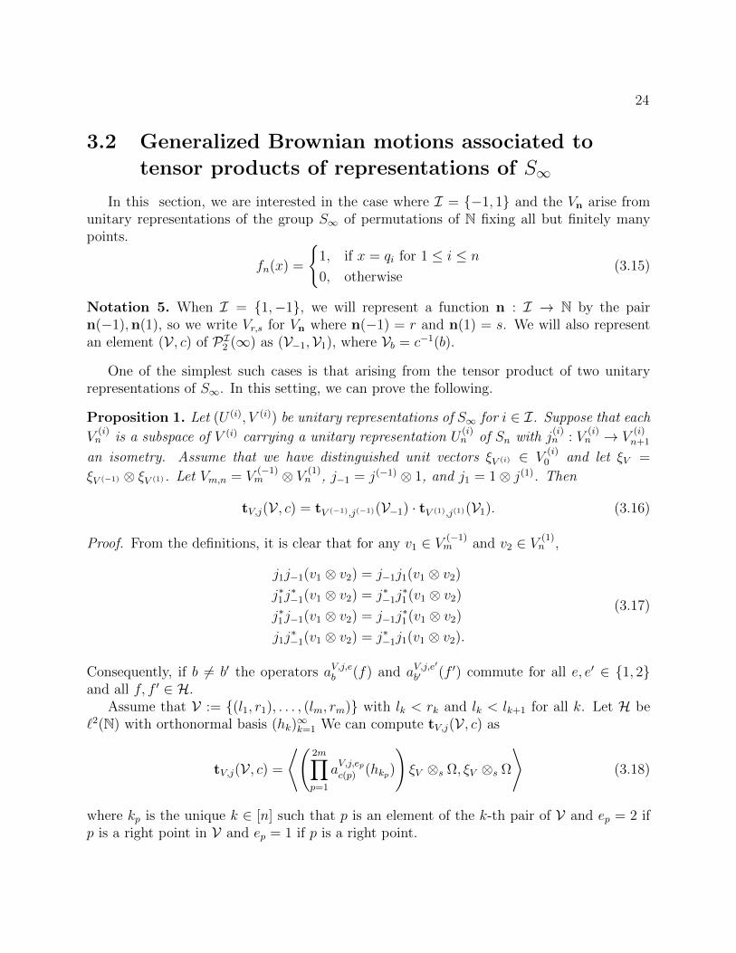
One of the simplest such cases is that arising from the tensor product of two unitaryrepresentations of S∞. In this setting, we can prove the following.

Proposition 1. Let (U (i), V (i)) be unitary representations of S∞ for i ∈ I. Suppose that each

V(i)n is a subspace of V (i) carrying a unitary representation U

(i)n of Sn with j

(i)n : V

(i)n → V

(i)n+1

an isometry. Assume that we have distinguished unit vectors ξV (i) ∈ V(i)

0 and let ξV =

ξV (−1) ⊗ ξV (1). Let Vm,n = V(−1)m ⊗ V (1)

n , j−1 = j(−1) ⊗ 1, and j1 = 1⊗ j(1). Then

tV,j(V , c) = tV (−1),j(−1)(V−1) · tV (1),j(1)(V1). (3.16)

Proof. From the definitions, it is clear that for any v1 ∈ V (−1)m and v2 ∈ V (1)

n ,

j1j−1(v1 ⊗ v2) = j−1j1(v1 ⊗ v2)

j∗1j∗−1(v1 ⊗ v2) = j∗−1j

∗1(v1 ⊗ v2)

j∗1j−1(v1 ⊗ v2) = j−1j∗1(v1 ⊗ v2)

j1j∗−1(v1 ⊗ v2) = j∗−1j1(v1 ⊗ v2).

(3.17)

Consequently, if b 6= b′ the operators aV,j,eb (f) and aV,j,e′

b′ (f ′) commute for all e, e′ ∈ 1, 2and all f, f ′ ∈ H.

Assume that V := (l1, r1), . . . , (lm, rm) with lk < rk and lk < lk+1 for all k. Let H be`2(N) with orthonormal basis (hk)

∞k=1 We can compute tV,j(V , c) as

tV,j(V , c) =

⟨(2m∏p=1

aV,j,epc(p) (hkp)

)ξV ⊗s Ω, ξV ⊗s Ω

⟩(3.18)

where kp is the unique k ∈ [n] such that p is an element of the k-th pair of V and ep = 2 ifp is a right point in V and ep = 1 if p is a right point.

25

Now, using the fact that aerc(p)(hkp) commutes with aep′

c(p′)(hkp′ ) when c(p) 6= c(p′), we have

tV,j(V , c) =

⟨ ∏c(p)=−1

aV,j,ep−1 (hkp)

∏c(p)=1

aV,j,ep1 (hkp)

ξV ⊗s Ω, ξV ⊗s Ω

⟩

=∏b∈I

⟨ ∏c(p)=b

aV (b),j(b),epb (hkp)ξV (b) ⊗s Ω, ξV (b) ⊗s Ω

⟩= tV (−1),j(−1)(V1) · tV (1),j(1)(V2).

(3.19)

This completes the proof.

Combining Theorem 7 with our Proposition 1 immediately gives the following.

Corollary 1. Let I = 1, 2. Fix (αi)∞i=1 and (βi)

∞i=1 decreasing sequences of positive real

numbers such that∑

i αi +∑

i βi ≤ 1 and let V(1)n = V

(2)n = V

(α,β)n with the Vershik-Kerov

representation of Sn. For i ∈ 1, 2, let j(i) : V(i)n → V

(i)n+1 be the natural isometry. Let

ξV (i) = 10 and let ξV = ξV (1) ⊗ ξV (2). Let Vm,n = V(−1)m ⊗ V

(1)n , j−1 = j(−1) ⊗ 1, and

j1 = 1⊗ j(1). Then for (V , c) ∈ PI2 (∞),

tV,j(V , c) =∏m≥2

(∞∑i=1

αmi + (−1)m+1

∞∑i=1

βmi

)ρm(V1)+ρm(V2)

(3.20)

26

Chapter 4

Generalized Brownian motionsassociated to spherical representationsof (S∞ × S∞, S∞)

In this chapter, we again use the index set I = −1, 1. Of course, we could have takenI to be any two-element set, but we have chosen −1, 1 for the reason that if b ∈ I thenwe can concisely refer to the other index as −b ∈ I.

Notation 6. With I = −1, 1, we will represent a function n : I → N by the pairn(−1),n(1), so we write Vr,s for Vn where n(−1) = r and n(1) = s.

G. Olshanski initiated the study of a broad class of representations of infinite symmetricgroups [Ols90], and this study has been further developed by Okounkov [Oko97]. In thisframework, one considers unitary representations of a pair of groups K ⊂ G forming aGelfand pair. Two groups (G,K) form a Gelfand pair if for every unitary representation(T,H) of G, the operators PKT (g)PK commute with each other as g ranges over G. HerePK denotes the orthogonal projection of H onto the subspace of K-invariant vectors for therepresentation T .

Of interest to us are the spherical representations, which are defined as irreducible unitaryrepresentations of G with a nonzero K-fixed vector ξ. If T is such a representation of thepair (G,K), then the function g 7→ 〈ξ, T (g)ξ〉 is called a spherical function of (G,K). Herewe consider the case where G = S∞ × S∞ and K = S∞ is the diagonal subgroup. It iswell-known (c.f. [Ols90]) that the finite factor representations of a discrete group G are inbijective correspondence with the spherical representations of the Gelfand pair (G×G,G),where G is a subgroup of G×G by the diagonal embedding.

In light of Thoma’s Theorem (Theorem 5) this means that the spherical functions of(S∞ × S∞, S∞) are parametrized by the Thoma parameters and that the spherical function

27

associated to the pairs (αi)∞i=1 and (βi)

∞i=1 is given by the formula

χα,β (π, π′) = φα,β(π′π−1

)=∏m≥2

(∞∑i=1

αmi + (−1)m+1

∞∑i=1

βmi

)ρm(π′π−1)

. (4.1)

For the generalized Brownian motion construction, we can consider the following data.Let (αi)

∞i=1 and (βi)

∞i=1 be a Thoma parameter. That is, let (αi)

∞i=1 and (βi)

∞i=1 be decreasing

sequences of positive real numbers such that∑

i αi +∑

i βi ≤ 1. Given n−1, n1 ∈ N∪0 letn = max(n−1, n1) and define

Vn−1,n1 = V (α,β)n , (4.2)

where V(α,β)n is as in (3.2). Then Vn−1,n1 carries a natural representation of Sn × Sn defined

by(U (α,β)

n (σ, π)h)(x, y) = (−1)i(σ,x)+i(π,y)h(σ−1x, π−1y), (4.3)

and thus a representation of Sn−1×Sn1 considering Sn−1×Sn1 as a subgroup of Sn×Sn. Forn−1 = n1, it is easy to see that the indicator function of the diagonal is fixed by the diagonalsubgroup.

Moreover, we define the map j−1 : Vn−1,n1 → Vn−1+1,n1 to be the natural embedding.When

∑αi +

∑βi = 1, this means that j−1 is given by

j−1δ(x(−1),x(1)) =

δ(x(−1),x(1)), if n1 > n−1,∑

z∈Q δ((x(−1)1 ,...,x

(−1)n ,z),(x

(1)1 ,...,x

(1)n ,z))

, otherwise.(4.4)

Likewise, we define the map j1 : Vn−1,n1 → Vn−1,n1+1 to be the natural embedding.We will also need to make use of the maps j∗b for b ∈ I. The map j∗−1 is given by

j∗−1δ(x(−1),x(1)) =

δ(x(−1),x(1)), if n1 ≥ n−1,

µ(x

(−1)n

)δx(−1)n ,x

(1)nδ((

x(−1)1 ,...,x

(−1)n−1

),(x(1)1 ,...,x

(1)n−1

)), otherwise.(4.5)

Here x(n−1) refers to the first n− 1 terms of the n-tuple (x1, . . . , xn−1−1) and the measure µis as in Notation 4. The maps j∗1 are defined analogously.

To motivate our results in the 2-colored case, we will consider another interpretation ofthe cycle decomposition of a pair partition. This interpretation involves some graph theory.We assume that a reader is familiar with the notion of a directed graph, a subgraph of adirected graph, and a cycle in a directed graph. These definitions can be found, for instance,in [BJG09]. For a subgraph H of G, we write V (H) to mean the vertex set of H and A(H)to mean the arc set of H.

Given a pair partition V ∈ P2(2m), we define a directed graph GV with vertex set [2m].For each (l, r) ∈ V with l < r, we add an arc (l, r) to GV . For each (l′, r′) ∈ V (as defined inDefinition 6) with l′ < r′, we add an arc (r′, l′) to GV .

28

The directed graph GV is the union of vertex-disjoint cycles, and the cycles of the graphGV give the cycles of the pair partition V . More precisely, if C is a cycle of GV then A(C)∩Vis a cycle of V . In particular, this means that ρm(V) is the number of cycles of GV of length2m.

Definition 7. For a directed graph G whose vertex set V has a total order <, an increasingpath P in G is a sequence of arcs (s1, s2), (s2, s3), . . . , (sr, sr+1) of G such that s1 < s2 <· · · < sr+1. We call r the length of P . A maximal increasing path in G is an increasing pathwhich is not contained in any increasing path in G of greater length. We define the notionsof decreasing paths and maximal decreasing paths in G analogously. A monotone path is apath which is either increasing or decreasing, and a maximal monotone path is a monotonepath which is not contained in any longer monotone path.

In the directed graph GV , each arc is a maximal monotone path, so the length of a cycleis the same as the number of maximal increasing paths in that cycle.

Combining with Theorem 7,

tα,β(V) =∏m≥2

(∞∑i=1

αmi + (−1)m+1

∞∑i=1

βmi

)γm(GV )

. (4.6)

where γm(GV) denotes the number of cycles of GV having m maximal increasing paths.The case of a 2-colored pair partition is naturally more complicated. As in the uncolored

case, our function on 2-colored pair partitions (V , c) will be calculated with the aid of thecycle decomposition of a directed graph (denoted GV,c), but the construction of a graphfrom a 2-colored pair partition will be rather more involved. However, in the case that thecoloring function is the constant function c(l, r) = 1, the graph GV,c will be identical to thegraph GV just described.

Before defining the graph GV,c we fix some notation.

Notation 7. For (V , c) ∈ PI2 (∞) with V = (l1, r1), · · · , (lm, rm), let LV := l1, . . . , ln bethe set of left points and RV := r1, . . . , rn denote the set of right points. If c : V → −1, 1is a coloring function, define for b ∈ I the functions

pbV,c : [0, 2m+ 1]→ N ∪ 0pbV,c(u) = |j ∈ [n] : lj ≤ u ≤ rj, c(lj, rj) = b|

(4.7)

Also definepV,c(u) = maxp−1

V,c(u), p1V,c(u) and rV,c(u) = p

c(u)V,c (u). (4.8)

Remark 5. In terms of the diagrams (e.g. Figure 2.1), pbV,c(m) is the number of b-coloredpaths intersecting the vertical line drawn through m (provided that the diagrams are drawnso as to minimize this quantity). Furthermore, rV,c(m) is the number of paths of the samecolor as m which intersect the vertical line drawn through m (provided that the diagramsare drawn so as to minimize this quantity).

29

The following properties are immediate consequences of the definitions and will be usedfrequently.

Proposition 2. Suppose that (V , c) ∈ BPI2 (∞), V = (l1, r1), . . . , (lm, rm) and b ∈ I =−1, 1.

1. If k ∈ [2m] and pbV,c(k) > pbV,c(k − 1) then c(k) = b and k ∈ LV .

2. If k ∈ [2m] and pbV,c(k + 1) < pbV,c(k) then c(k) = b and k ∈ RV .

3. If k ∈ [2m+ 1] then pbV,c(k)− pbV,c(k − 1) ∈ −1, 0, 1.

4. If k, k′ ∈ [0, 2m + 1] with k < k′, pbV,c(k) < pbV,c(k′) and u ∈ [pbV,c(k), pbV,c(k

′)], thenthere is some l ∈ [k, k′] such that pbV,c(l) = u.

5. If k, k′ ∈ [0, 2m + 1] with k < k′, pbV,c(k) > pbV,c(k′) and u ∈ [pbV,c(k

′), pbV,c(k)], thenthere is some l ∈ [k, k′] such that pbV,c(l) = u.

6. If k ∈ LV and k ∈ [2m] then rV,c(k) ≥ pc(k)V,c (k − 1) and pbV,c(k) ≥ pbV,c(k + 1) for b ∈ I.

7. If k ∈ RV and k ∈ [2m] then rV,c(k) ≥ pc(k)V,c (k + 1) and pbV,c(k) ≥ pbV,c(k − 1) for b ∈ I.

We need some additional notation.

Notation 8. For an I-indexed pair partition (V , c), define

DV,c = k ∈ [2m] : rV,c(k) > p−c(k)V,c (k)

SV,c = [2m] \ DV,c.(4.9)

The next remark should clarify the importance of these terms.

Remark 6. If (V , c) ∈ PI2 (2n) then by (2.5), tα,β(V , c) can be computed by evaluating thevacuum state at a word in creation and annihilation operators. More precisely, we can write

tα,β(V , c) = 〈ξV α,β ⊗ Ω, A1 · · ·A2n (ξV α,β ⊗ Ω)〉 (4.10)

where Ak is a creation operator if k ∈ RV,c and an annihilation operator if k ∈ LV,c. Ineither case, the color of the operator Ak is c(k). One can characterize these operators moreprecisely, but we will not need to do so at this point.

For any k ∈ [2n], the vector (Ak+1 · · · · · A2n) ξV α,β ⊗ Ω lies in the space V α,βnk⊗H⊗nk for

some function nk : I → Z. A c(k)-colored creation operator maps the space V α,βnk⊗H⊗nk to

V α,βnk+δc(k)

⊗H⊗nk+δc(k) . If k ∈ RV , then k ∈ SV,c if and only if the transition map

jc(k) : V α,βnk→ V α,β

nk+δc(k)(4.11)

is the identity map on V α,βnk

, where nk = maxnk(b) : b ∈ I. The analogous statement alsoholds for k ∈ LV .

30

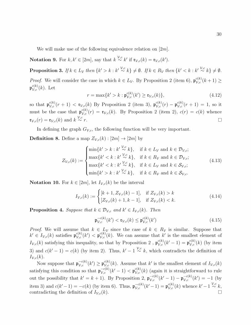
We will make use of the following equivalence relation on [2m].

Notation 9. For k, k′ ∈ [2m], say that kV,c∼ k′ if rV,c(k) = rV,c(k

′).

Proposition 3. If k ∈ LV then k′ > k : k′V,c∼ k 6= ∅. If k ∈ RV then k′ < k : k′

V,c∼ k 6= ∅.

Proof. We will consider the case in which k ∈ LV . By Proposition 2 (item 6), pc(k)V,c (k + 1) ≥

pc(k)V,c (k). Let

r = maxk′ > k : pc(k)V,c (k′) ≥ rV,c(k), (4.12)

so that pc(k)V,c (r + 1) < rV,c(k) By Proposition 2 (item 3), p

c(k)V,c (r) − p

c(k)V,c (r + 1) = 1, so it

must be the case that pc(k)V,c (r) = rV,c(k). By Proposition 2 (item 2), c(r) = c(k) whence

rV,c(r) = rV,c(k) and kV,c∼ r.

In defining the graph GV,c, the following function will be very important.

Definition 8. Define a map ZV,c(k) : [2m]→ [2m] by

ZV,c(k) :=

mink′ > k : k′

V,c∼ k, if k ∈ LV and k ∈ DV,c;maxk′ < k : k′

V,c∼ k, if k ∈ RV and k ∈ DV,c;maxk′ < k : k′

V,c∼ k, if k ∈ LV and k ∈ SV,c;mink′ > k : k′

V,c∼ k, if k ∈ RV and k ∈ SV,c.

(4.13)

Notation 10. For k ∈ [2m], let IV,c(k) be the interval

IV,c(k) :=

[k + 1, ZV,c(k)− 1], if ZV,c(k) > k

[ZV,c(k) + 1, k − 1], if ZV,c(k) < k.(4.14)

Proposition 4. Suppose that k ∈ DV,c and k′ ∈ IV,c(k). Then

p−c(k)V,c (k′) < rV,c(k) ≤ p

c(k)V,c (k′) (4.15)

Proof. We will assume that k ∈ LV since the case of k ∈ RV is similar. Suppose thatk′ ∈ IV,c(k) satisfies p

c(k)V,c (k′) < p

c(k)V,c (k). We can assume that k′ is the smallest element of

IV,c(k) satisfying this inequality, so that by Proposition 2 , pc(k)V,c (k′ − 1) = p

c(k)V,c (k) (by item

3) and c(k′ − 1) = c(k) (by item 2). Thus, k′ − 1V,c∼ k, which contradicts the definition of

IV,c(k).

Now suppose that p−c(k)V,c (k′) ≥ p

c(k)V,c (k). Assume that k′ is the smallest element of IV,c(k)

satisfying this condition so that p−c(k)V,c (k′ − 1) < p

c(k)V,c (k) (again it is straightforward to rule

out the possibility that k′ = k + 1). By Proposition 2, p−c(k)V,c (k′ − 1) − p

−c(k)V,c (k′) = −1 (by

item 3) and c(k′−1) = −c(k) (by item 6). Thus, p−c(k)V,c (k′−1) = p

c(k)V,c (k) whence k′−1

V,c∼ k,contradicting the definition of IV,c(k).

31

Proposition 5. If k ∈ SV,c and k′ ∈ IV,c(k) then

pc(k)V,c (k′) < p

−c(k)V,c (k) ≤ p

−c(k)V,c (k′). (4.16)

Proof. We will again assume that k ∈ LV as the case of k ∈ RV is similar. Suppose thatk′ ∈ IV,c(k) is such that p

c(k)V,c (k′) ≥ p

−c(k)V,c (k). Assume that k′ is the largest element of IV,c(k)

satisfying this inequality. One can check that if k′ = k − 1 then k − 1V,c∼ k and IV,c(k) = ∅,

so we assume that k′ + 1 ∈ IV,c(k) and thus pc(k)V,c (k′ + 1) < p

−c(k)V,c (k). By Proposition 2, it

follows that pc(k)V,c (k′ + 1) − p

c(k)V,c (k′) = −1 and c(k′ + 1) = c(k). Thus, k′ + 1

V,c∼ k, whichcontradicts the definition of IV,c(k).

Now suppose that there is some k′ ∈ IV,c(k) such that p−c(k)V,c (k′) < p

−c(k)V,c (k). Again

assume that k′ is the largest element of IV,c(k) satisfying this inequality. Since p−c(k)V,c (k−1) ≥

p−c(k)V,c (k), we must have k 6= k − 1, so that k′ ∈ IV,c(k) and p

−c(k)V,c (k′ + 1) > p

−c(k)V,c (k). By

Proposition 2, p−c(k)V,c (k′ + 1)− p

−c(k)V,c (k) = 1 and c(k′ + 1) = −c(k). But also p

−c(k)V,c (k′ + 1) =

pc(k)V,c (k) whence k′ + 1

V,c∼ k, contradicting the definition of IV,c(k).

Proposition 6. Suppose that (V , c) ∈ PI2 (2m) and k ∈ [2m]. Then the following hold:

1. If k ∈ DV,c then ZV,c(k) ∈ DV,c if and only if c(k) = c(ZV,c(k));

2. If k ∈ SV,c then ZV,c(k) ∈ SV,c if and only if c(k) = c(ZV,c(k));

3. If k ∈ LV then ZV,c(k) ∈ LV if and only if c(ZV,c(k)) = −c(k);

4. If k ∈ RV then ZV,c(k) ∈ RV if and only if c(ZV,c(k)) = −c(k);

5. ZV,c(ZV,c(k)) = k.

Proof. We fix an I-indexed pair partition (V , c). For compactness and readability, we willabbreviate ZV,c(k) by k∗.

If k ∈ LV ∩ DV,c then by definition k∗ > k. By Proposition 4,

p−c(k)V,c (k∗ − 1) < rV,c(k) < p

c(k)V,c (k∗ − 1). (4.17)

Using the fact that k∗V,c∼ k and applying Proposition 2, it follows that if c(k∗) = c(k) then

k∗ ∈ RV and k∗ ∈ DV,c whereas if c(k∗) = c(−k) then k∗ ∈ LV and k∗ ∈ SV , c.If k ∈ LV ∩ SV,c then by definition k∗ < k. By Proposition 5,

pc(k)V,c (k∗ + 1) < p

−c(k)V,c (k) < p

−c(k)V,c (k∗ + 1). (4.18)

Using the fact that k∗V,c∼ k and applying Proposition 2, it follows that if c(k∗) = c(k) then

k∗ ∈ RV and k∗ ∈ SV,c whereas if c(k∗) = c(−k) then k∗ ∈ LV and k∗ ∈ DV,c.Collecting all of these cases, as well as the analogous statements for k ∈ RV gives items

1, 2, 3, and 4. Making use of the definition of ZV,c, it follows that (k∗)∗ < k∗ if and only ifk < k∗, whence k = (k∗)∗.

32

Corollary 2. If (V , c) ∈ PI2 (2m) then the function ZV,c : [2m] → [2m] defines a pairpartition V(c) ∈ PI2 (2m) by

V(c) := (k, ZV,c(k)) : k < ZV,c(k) . (4.19)

We define a coloring function on V(c) by:

c (k, ZV,c(k)) =

c(k), if k ∈ SV,c−c(k), if k ∈ DV,c.

(4.20)

Remark 7. This definition of c (k, ZV,c(k)) does not depend on which point of a pair is chosenas k because c(k) = c(ZV,c(k)) if and only if k and ZV,c(k) are either both in SV,c or both inDV,c.

Notation 11. Define a map (·, ·)(−1) on [2m] × [2m] by (u, v)(−1) = (v, u). Also let (·, ·)(1)

be the identity map on [2m]× [2m].

We are now ready to define the graph GV,c.

Definition 9. If (V , c) ∈ PI2 (2m), then GV,c is the directed graph with vertices [2m] andarcs defined as follows. Let

FV,c = (l, r)(c(l,r)) : (l, r) ∈ VFV,c = (k, k′)(c(k,k′)) : (k, k′) ∈ V(c).

(4.21)

The graph GV,c has arc setAV,c := FV,c ∪ FV,c (4.22)

Proposition 7. The sets FV,c and FV,c have empty intersection.

Proof. We need only show that if (l, r) ∈ V with ZV,c(l) = r then c(l, r) = −c(l, r). By thedefinition of c, it will suffice to show that l ∈ DV,c. Since l < ZV,c(l), ZV,c(l) = r ∈ RV andc(l) = c(ZV,c(l)), this follows from Proposition 6 and the definition of ZV,c.

Example 3. We consider the example of the graph GV,c for the I-indexed pair partition(V , c) with

V = (1, 5), (2, 10), (3, 8), (6, 7), (4, 12), (9, 11);c(1, 5) = c(2, 9) = c(8, 10) = c(6, 7) = −1;

c(3, 8) = c(4, 12) = 1.

(4.23)

The I-indexed pair partition (V , c) is depicted in Figure 4.1.We can determine the values of p−1

V,c(k) and p1V,c(k) by drawing a vertical line through the

diagram at k and counting the intersections with paths of the respective colors. For instance,

33

1 2 3 4 5 6 7 8 9 10 11 12

Figure 4.1: The −1, 1-indexed pair partition (V , c) given in (4.23).

1 2 3 4 5 6 7 8 9 10 11 12

Figure 4.2: The I-indexed pair partition (V(c), c) where (V , c) is the pair partition depictedin the Figure 4.1.

a vertical line through k = 3 intersects 2 solid paths and 1 dotted path (at the endpoint),

so p(1)V,c(3) = 1 and p

(−1)V,c (3) = −1. Since c(3) = 1, this means that 3 ∈ SV,c.

Repeating the process for the other elements of [12] we can fill in the first few rows of

Table 4.1. From the data, one sees that the equivalence class of 3 underV,c∼ is 1, 3, 11, 12

whenceZV,c(3) = 1. (4.24)

Continuing in this way for other elements of 2m, the pair partition V(c) is given by

V(c) := (1, 3), (2, 4), (5, 6), (7, 8), (9, 10), (11, 12) (4.25)

and the color function c : V(c) → I is given by

c(5, 6) = c(7, 8)) = c(11, 12) = −1;

c(1, 3) = c(2, 4)) = c(9, 10) = 1.(4.26)

This I-indexed broken pair partition is depicted in Figure 4.2.Accordingly, the sets FV,c and FV,c are given by

FV,c = (5, 1), (10, 2), (3, 8), (4, 12), (7, 6), (11, 9)FV,c = (6, 5), (12, 11), (1, 3), (2, 4), (7, 8), (9, 10)

(4.27)

The directed graph GV,c is depicted in Figure 4.3.

Proposition 8. Let (V , c) ∈ PI2 (∞) be a −1, 1-colored pair partition. Then the graphGV,c is the union of vertex-disjoint directed cycles.

Proof. Let m = |V|. It is an immediate consequence of the definition of GV,c that for eachk ∈ [2m] there are exactly two arcs having k as either the start point or the end point. We

34

k c(k) r(V,c)(k) p−c(k)(V,c) (k) DV,c or SV,c Z(V,c)(k)

1 -1 1 0 DV,c 32 -1 2 0 DV,c 43 1 1 2 SV,c 14 1 2 2 SV,c 25 -1 2 2 SV,c 66 -1 2 2 SV,c 77 -1 2 2 SV,c 88 1 2 1 DV,c 79 -1 2 1 DV,c 1010 -1 2 1 DV,c 911 -1 1 1 SV,c 1212 -1 1 1 DV,c 11

Table 4.1: Data pertaining to the I-indexed pair partition depicted in Figure 2.5.

1 2 3 4 5 6 7 8 9 10 11 12

Figure 4.3: The directed graph GV,c for the −1, 1-colored pair partition depicted in Figure4.1. The graph GV,c has 2 cycles, one with vertex set 1, 3, 8, 7, 6, 5 and one with vertex set2, 4, 12, 11, 9, 10. The former cycle has one maximal increasing path, and the latter has 2maximal increasing paths.

must show that each vertex k ∈ [2m] is the starting point of one edge and the end point ofanother edge.

We will assume k ∈ LV , so that (k, r) ∈ V for some r ∈ [2m]. If k ∈ DV,c thenZV,c(k) > k, so (k, ZV,c(k)) ∈ V(c). Since c(k, r) = −c(k, ZV,c(k)), k is the starting point ofexactly one of these arcs. If k ∈ SV,c then ZV,c(k) < k, so (ZV,c(k), k) ∈ V(c). Furthermore,c(k, r) = c(ZV,c(k), k), whence k is again the starting point of exactly one of the arcs.

Remark 8. If c(d) = 1 ∈ I for every d ∈ V then every DV,c = [2m] and V(c) = V (where V isas in Definition 6) with c(d) = −1 for all d ∈ V(c). Thus GV,c = GV .

A cycle C in the graph GV,c can be decomposed into maximal monotone paths (Definition7). That is, there are maximal monotone paths P1, . . . , Ps such that each arc of C lies alongexactly one of the Pj.

35

Notation 12. For a directed graph G on a totally ordered vertex set, we denote by γm(G) thenumber of cycles of G having exactly m maximal increasing paths (equivalently, m maximaldecreasing paths).

With this established, we are able to state the main result of this section.

Theorem 8. Let (αi)∞i=1 and (βi)

∞i=1 be decreasing sequences of positive real numbers such

that∑

i αi +∑

i βi ≤ 1. Let V(α,β)n−1,n1 be the complex Hilbert space of the Vershik-Kerov

representation of Smax(n−1,n1) endowed with the representation of (4.3), and let

j−1n : V (α,β)

n−1,n1→ V

(α,β)n−1+1,n1

and j1n : V (α,β)

n−1,n1→ V

(α,β)n−1,n1+1 (4.28)

be the natural embedding. Let ξV (α,β) = 10 be the indicator function of the diagonal. Denoteby tα,β the function on PI2 (∞) associated to this sequence of representations by Theorem 1.

Let (V , c) be a −1, 1-colored pair partition. Then

tα,β(V , c) =∏m≥2

(∞∑i=1

αmi + (−1)m+1

∞∑i=1

βmi

)γm(GV,c)

. (4.29)

We will present the proof of Theorem 8 in the case that∑

n αn = 1. This case willcontain the key ideas of the more general argument, but will simplify notation considerablyand allow us to consider discrete sums instead of integrals.

Notation 13. For (V , c) ∈ PI2 (2m), define

RDV,c := k ∈ RV : k ∈ DV,c

LDV,c := k ∈ LV : k ∈ DV,c.(4.30)

Proposition 9. Let I = −1, 1 and let (V , c) ∈ PI2 (2m). Every maximal increasing path in(V , c) has its starting point in LDV,c and its terminal point in RD

V,c. Every maximal decreasingpath in (V , c) has its starting point in RD

V,c and its terminal point in LDV,c.

Proof. This follows immediately from the definitions of the map ZV,c and the graph GV,c. Aleft point l ∈ LDV,c, is adjacent to vertices u, v with l < u and l < v whereas if l ∈ LV ∈ SV,c,l is adjacent to one vertex u′ with u′ < l and another vertex v′ with l < v′.

The proof of Theorem 8 will be aided by some additional terminology.

Definition 10. Let H be an infinite-dimensional complex Hilbert space with orthonormalbasis B := hi∞i=1. We will say that a vector η ∈ FV (H) is B-elementary if there is aconstant C, and some n−1, n1 such that there is a pair of tuples x(−1), x(1) ∈ Xn of lengthn := max(n−1, n1) with x(−1) ∼ x(1) (where Xn and the relation ∼ are as in Notation 4) and

indices i(−1)1 , . . . , i

(−1)n−1 ∈ N and i

(1)1 , . . . , i

(1)n1 ∈ N all distinct such that

η = C · δ(x(−1),x(1)) ⊗s hi(−1)1⊗ · · · ⊗ h

i(−1)n−1

⊗ hi(1)1⊗ · · · ⊗ h

i(1)n1

. (4.31)

Denote by EBV (H) the set of all B-elementary vectors in FV (H).

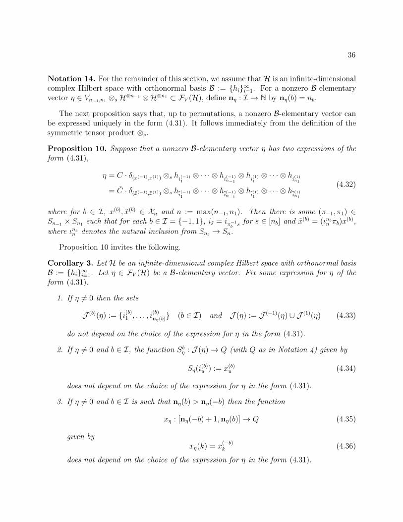
36

Notation 14. For the remainder of this section, we assume that H is an infinite-dimensionalcomplex Hilbert space with orthonormal basis B := hi∞i=1. For a nonzero B-elementaryvector η ∈ Vn−1,n1 ⊗s H⊗n−1 ⊗H⊗n1 ⊂ FV (H), define nη : I → N by nη(b) = nb.

The next proposition says that, up to permutations, a nonzero B-elementary vector canbe expressed uniquely in the form (4.31). It follows immediately from the definition of thesymmetric tensor product ⊗s.

Proposition 10. Suppose that a nonzero B-elementary vector η has two expressions of theform (4.31),

η = C · δ(x(−1),x(1)) ⊗s hi(−1)1⊗ · · · ⊗ h

i(−1)n−1

⊗ hi(1)1⊗ · · · ⊗ h

i(1)n1

= C · δ(x(−1),x(1)) ⊗s hi(−1)1⊗ · · · ⊗ h

i(−1)n−1

⊗ hi(1)1⊗ · · · ⊗ h

i(1)n1

(4.32)

where for b ∈ I, x(b), x(b) ∈ Xn and n := max(n−1, n1). Then there is some (π−1, π1) ∈Sn−1 × Sn1 such that for each b ∈ I = −1, 1, is = iπ−1

b s for s ∈ [nb] and x(b) = (ιnbn πb)x(b),

where ιnbn denotes the natural inclusion from Snb → Sn.

Proposition 10 invites the following.

Corollary 3. Let H be an infinite-dimensional complex Hilbert space with orthonormal basisB := hi∞i=1. Let η ∈ FV (H) be a B-elementary vector. Fix some expression for η of theform (4.31).

1. If η 6= 0 then the sets

J (b)(η) := i(b)1 , . . . , i(b)nη(b) (b ∈ I) and J (η) := J (−1)(η) ∪ J (1)(η) (4.33)

do not depend on the choice of the expression for η in the form (4.31).

2. If η 6= 0 and b ∈ I, the function Sbη : J (η)→ Q (with Q as in Notation 4) given by

Sη(i(b)u ) := x(b)

u (4.34)

does not depend on the choice of the expression for η in the form (4.31).

3. If η 6= 0 and b ∈ I is such that nη(b) > nη(−b) then the function

xη : [nη(−b) + 1,nη(b)]→ Q (4.35)

given byxη(k) = x

(−b)k (4.36)

does not depend on the choice of the expression for η in the form (4.31).

37

4. Moreover,

D(η) =

0, if η = 0

C, if η 6= 0 is expressed in the form (4.31)(4.37)

does not depend on the choice of the expression for η in the form (4.31).

We can now characterize the effect of an annihilation operator on a B-elementary vector.In doing so, it will be convenient to fix the Hilbert spaces Vn and the transition maps jband omit the superscripts V and j. The next two propositions follow immediately from thedefinition of the annihilation operators.

Proposition 11. If η ∈ FV (H) is a B-elementary vector and b ∈ I is such that nη(b) >

nη(−b) and i ∈ J (b)η , then ab(hi)η is also a B-elementary vector and

D(ab(hi)η) =δxη(nη(b)),Sη(i) · µ(Sη(i))

nη(b)·D(η). (4.38)

Furthermore if ab(hi)η 6= 0, then the following hold:

1. J (b)(ab(hi)η) = J (b)(η) \ i;

2. J (−b)(ab(hi)η) = J (−b)(η);

3. For i′ ∈ [nη(−b) + 1,nη(b)− 1], xab(hi)η(nη(b)) = xη(nη(b));

4. For any i′ ∈ J (ab(hi)η) = J (η) \ i, Sab(hi)η(i′) = Sη(i′).

Proposition 12. Let η ∈ FV (H) be a nonzero B-elementary vector. Fix i ∈ Jη, and letb ∈ I be such that nη(b) ≤ nη(−b). Then ab(hi)η is a B-elementary vector and

D(ab(hi)η) =1

nη(b)·D(η). (4.39)

If ab(hi)η 6= 0 then the following also hold:

1. J (b)(ab(hi)η) = J (b)(η) \ i;

2. J (−b)(ab(hi)η) = J (−b)(η);

3. For i′ ∈ [nη(b) + 1,nη(b)], xab(hi)η(nη(b)) = xη(nη(b));

4. xab(hi)η(nη(b)) = Sη(i);

5. For any i′ ∈ J (ab(hi)η) = J (η) \ i, Sab(hi)η(i′) = Sη(i′).

A creation operator need not take a B-elementary vector to another B-elementary vector.However, we can express a creation operator as a sum of operators which preserve the B-elementary property.

38

Notation 15. For z ∈ Q = N, let εz : Vn → Vn+1 to be the linear map such that εzδ(x,y) =δ((x,z),(y,z)). If h ∈ H and n−1 ≥ n1 define an operator

a∗−1,z(hr) : Vn−1 ⊗s H⊗n−1 ⊗H⊗n1 → Vn−1+1 ⊗s H⊗n−1+1 ⊗H⊗n1 (4.40)

bya∗−1,z(hr)η = (nη(b)εz ⊗ r−1(h)) η. (4.41)

Define a∗1,z(hr) similarly for n1 ≥ n−1.

Remark 9. In the case that∑αi = 1 (and thus βi = 0 and γ = 0), we have∑

z∈Q

a∗b,z(h)η = a∗b(h)η (4.42)

for a B-elementary vector η ∈ F(V ) with nη(b) > nη(−b).The following two propositions follow directly from the definition of the respective oper-

ators.

Proposition 13. If η ∈ FV (H) is a B-elementary vector, b ∈ I is such that nη(b) ≥ nη(−b),and i ∈ N\J (η) then for any z ∈ Q, the vector a∗b,z(hi)η is also B-elementary. Furthermore,the following hold:

1. If η 6= 0 then J (b)(a∗b,z(hi)η) = J (b)(η) ∪ i;

2. If η 6= 0 then J (−b)(a∗−b,z(hi)η) = J (−b)(η);

3. For any i′ ∈ J (η), Sa∗b,z(hi)η(i′) = Sη(i

′);

4. Sa∗b,z(hi)η(i) = z;

5. D(a∗b,z(hi)η) = (nη(b) + 1) ·D(η).

Proposition 14. If η ∈ FV (H) is a B-elementary vector, b ∈ B is such that nη(−b) > nη(b),and i ∈ N \ Jη then the vector a∗b(hi)η is also B-elementary. Furthermore,

1. If η 6= 0 then J (b)(a∗b(hi)η) = J (b)(η) ∪ i;

2. If η 6= 0 then J (−b)(a∗−b(hi)η) = J (−b)(η);

3. For any i′ ∈ J (η), Sa∗b,z(hi)η(i′) = Sη(i

′);

4. If η 6= 0 then Sa∗b (hi)η(i) = xη(nη(b)).

5. D(a∗b(hi)η) = (nη(b) + 1)D(η).

We are now ready to prove the main theorem.

39

Proof of Theorem 8. We reiterate that we are focusing on the case∑αi = 1 for simplicity.

The key ideas of the more general case∑αi +

∑βi ≤ 1 are in this case, but this case

is slightly more straightforward in that it allows us to work with discrete sums instead ofintegrals. In this case, we can assume that Q = N.

Let n = |V| and let H be an infinite-dimensional complex Hilbert space with an orthonor-mal basis B := hi∞i=1. By Theorem 1, we can compute tV,j(V , c) as

tV,j(V , c) =⟨ae1c(1)(hk1) · · · a

enc(n)(hkn) (10 ⊗s Ω) ,10 ⊗s Ω

⟩, (4.43)

where i is an element of the ki-th pair of V , and ei = 2 if i ∈ RV and ei = 1 if i ∈ LV . Foreach k ∈ [2m] define

Ai :=

a∗c(i)(hki), if i ∈ RVac(i)(hki), if i ∈ LV ,

(4.44)

so thattV,j(V , c) = 〈(A1 · · ·A2m) 10 ⊗s Ω,10 ⊗s Ω〉 , (4.45)

Denote by ΛV,c the space of functions λ : RDV,c → Q. For λ ∈ ΛV,c and i ∈ [2m], define

Aλ,i :=

a∗c(i),λ(i)(hki), if i ∈ RD

V,c

Ai, otherwise.(4.46)

We defineA

(k)λ := Aλ,k · · ·Aλ,2m (4.47)

for 1 ≤ k ≤ 2m. For convenience, we also set A(2m+1)λ = 1. It follows immediately from the

definitions and (4.45) that

tV,j(V , c) =∑λ∈ΛV,c

⟨A

(1)λ 10 ⊗s Ω,10 ⊗s Ω

⟩(4.48)

Also defineηλ,k := A

(k)λ 10 ⊗s Ω. (4.49)

It can be seen from the definition of pbV,c that if ηλ,k 6= 0 then

nηλ,k(b) =

p

(b)V,c(k)− 1, if k ∈ LV and c(k) = b,

p(b)V,c(k), otherwise.

(4.50)

for b ∈ I.It follows from Propositions 11, 12, 13 and 14 that ηλ,k is B-elementary for 1 ≤ k ≤ 2m+1.

Since ηλ,1 ∈ C10 ⊗s Ω, it is determined by the constant D(ηλ,1). For k ∈ [2m], define

Bλ,k :=

δxηλ,k+1

(nηλ,k+1(b)),Sηλ,k+1

(i) · µ(Sηλ,k+1(i)) if k ∈ LDV,c

1, otherwise,(4.51)

40

so that

D(ηλ,1) =2m∏k=1

Bλ,k =∏

k∈LDV,c

Bλ,k. (4.52)

For a maximal increasing path P of GV,c from ls to rt with ls < rt, define a functionHP,λ : [ls + 1, rt] → Q as follows. If u ∈ [ls + 1, rt], denote by fu = (au, zu) the unique arcalong the path P such that au < u ≤ zu. Then we define

HP,λ(u) :=

xηλ,u(rV,c(au)), if fu = (au, zu) ∈ Vc

Sηλ,u(i), if fu = (li, ri) ∈ V .(4.53)

It can be verified using (4.50) that if b ∈ I is such that pc(b)(au) > pc(−b)(au) and fu ∈ FV,cthen nηλ,u(b) < rV,c(au) ≤ nηλ,u(−b), so that rV,c(au) is indeed in the domain of xηλ,u .

We will show that HP,λ(u) = λ(ls) for all u ∈ [ls + 1, rt]. By definition,

ηλ,rt = Aλ,rtηλ,rt+1 = a∗c(rt),λ(rt)(ht)ηλ,rt+1. (4.54)

As an endpoint of a maximal monotone path, rt ∈ DV,c, and pc(rt)V,c (rt) > p

−c(rt)V,c (rt) implies

that nηλ,rt−1(c(rt)) > nηλ,rt+1

(−c(rt)). If frt ∈ FV,c then by Proposition 13,

HP,λ(rt) = xa∗c(rt),λ(rt)

(ht)ηλ,rt+1(rV,c(c(rt))) = λ(rt). (4.55)

If, on the other hand, fu = (lt, rt) ∈ V then

HP,λ(rt) = Sa∗c(rt),λ(rt)

(ht)ηλ,rt+1(t) = λ(rt), (4.56)

where we have again applied Proposition 13.To show that HP,λ(u) = λ(rt) for all u, it will now suffice to show that HP,λ(u) =

HP,λ(u+1) for u ∈ [ls+1, rt−1]. For u such that fu = fu+1 this is an immediate consequenceof the definition ofHP,λ(u). Otherwise, u is a vertex along the path P and u ∈ SV,c. If u ∈ LV ,say u = li, then (au, zu) = (u, zu) ∈ FV,c, thus

HP,λ(u) = xηλ,u(rV,c(c(au)))

= xac(u)(hi)ηλ,u+1(rV,c(c(au)))

= Sηλ,u+1(i)

= HP,λ(u+ 1).

(4.57)

Here we have made use of Proposition 12.If instead u ∈ RV , say u = ri, then (au, zu) = (li, ri) ∈ V , so

HP,λ(u) = Sηλ,u(i)

= Sa∗c(u)

(hi)ηλ,u+1(i)

= xηλ,u+1(nηλ,u+1

(c(u)))

= xηλ,u+1(rV,c(ri))

= HP,λ(u+ 1),

(4.58)

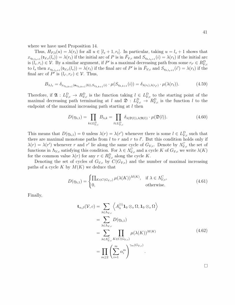
41

where we have used Proposition 14.Thus, HP,λ(u) = λ(rt) for all u ∈ [ls + 1, rt]. In particular, taking u = ls + 1 shows that

xηλ,ls+1(rV,c(ls)) = λ(rt) if the initial arc of P is in FV,c and Sηλ,ls+1

(i) = λ(rt) if the initial arcis (li, ri) ∈ V . By a similar argument, if P ′ is a maximal decreasing path from some rt′ ∈ RD

V,cto ls then xηλ,ls+1

(rV,c(ls)) = λ(rt) if the final arc of P ′ is in FV,c and Sηλ,ls+1(i′) = λ(rt) if the

final arc of P ′ is (li′ , ri′) ∈ V . Thus,

Bλ,ls = δxηλ,k+1(nηλ,k+1

(b)),Sηλ,k+1(i) · µ(Sηλ,k+1

(i)) = δλ(rt),λ(rt′ )· µ(λ(rt)). (4.59)

Therefore, if A : LDV,c → RDV,c is the function taking l ∈ LDV,c to the starting point of the

maximal decreasing path terminating at l and D : LDV,c → RDV,c is the function l to the

endpoint of the maximal increasing path starting at l then

D(ηλ,1) =∏

k∈LDV,c

Bλ,k =∏l∈LDV,c

δλ(D(l)),λ(A(l)) · µ(D(l)). (4.60)

This means that D(ηλ,1) = 0 unless λ(r) = λ(r′) whenever there is some l ∈ LDV,c such thatthere are maximal monotone paths from l to r and r to l′. But this condition holds only ifλ(r) = λ(r′) whenever r and r′ lie along the same cycle of GV,c. Denote by ΛC

V,c the set offunctions in ΛV,c satisfying this condition. For λ ∈ ΛC

V,c and a cycle K of GV,c we write λ(K)for the common value λ(r) for any r ∈ RD

V,c along the cycle K.Denoting the set of cycles of GV,c by C(GV,c) and the number of maximal increasing

paths of a cycle K by M(K) we deduce that

D(ηλ,1) =

∏K∈C(GV,c)

µ(λ(K))M(K), if λ ∈ ΛCV,c,

0, otherwise.(4.61)

Finally,

tα,β(V , c) =∑λ∈ΛV,c

⟨A

(1)λ 10 ⊗s Ω,10 ⊗s Ω

⟩=∑λ∈ΛV,c

D(ηλ,1)

=∑λ∈ΛCV,c

∏K∈C(GV,c)

µ(λ(K))M(K)

=∏m≥2

(∞∑i=1

αmi

)γm(GV,c)

.

(4.62)

42

Chapter 5

A special case of the generalizedBrownian motions associated tospherical representations of(S∞ × S∞, S∞)

In this chapter, we specialize the investigation begun in Chapter 4 to a countable classof Thoma parameters which were also considered in [BG02]. Namely, for N ∈ Z \ 0 wewill consider the spherical function ϕN of the Gelfand pair (S∞ × S∞, S∞) arising from theThoma parameters with

αn =

1/N, N > 0 and 1 ≤ n ≤ N ;

0, otherwise.and βn =

1/N, N < 0 and 1 ≤ n ≤ |N |;0, otherwise.

(5.1)

The character ϕN on S∞ is given by

ϕN(π) =

(1

N

)m−γ(m)(π)

(5.2)

where m is large enough so that σ(k) = k for k > m and γ(m) (σ) is the number of cyclesin the permutation σ ∈ S∞ when σ is considered as an element of Sm. Although γ(m) (σ)depends on the choice of m, the quantity m− γ(m) (σ) does not.

We denote by ψN the associated spherical function on the Gelfand pair (S∞ × S∞, S∞).That is,

ψN(π−1, π1) = ϕN(π−11 π−1) =

(1

N

)m−γ(m)(π−11 π−1)

, (5.3)

where (π−1, π1) ∈ S∞ × S∞.

43

The function on −1, 1-indexed pair partitions associated to ψN by Theorem 8 is givenby

tN(V , c) =

(1

N

)m(GV,c)−γ(GV,c)

, (5.4)

where m(GV,c) and γ(GV,c) denote the number of maximal increasing paths and number ofcycles of the graph GV,c defined in Chapter 4, respectively.

For a complex Hilbert space H, the function tN gives rise to a Fock state ρN on thealgebra CI(H). We denote by FIN(H), ΩN , and CIN(H) the Hilbert space, distinguishedcyclic vector, and algebra of operators of the GNS construction for this pair. We will seethat for N < 0, the field operators on FN(H) are bounded operators which generate a vonNeumann algebra containing the projection onto vacuum vector.

Notation 16. Fix an integer N 6= 0 and an infinite-dimensional complex Hilbert space Hwith orthonormal basis B := hn : n ∈ N. Denote by a∗b,i the creation operator a∗tN ,b(hi)and by ab,i the annihilation operator atN ,b(hi). As we have done before, we will write aeb,i foreither a creation (e = 2) or annihilation operator (e = 1) and let ωb,i = ab,i+a∗b,i. Let ΓIN(H)be the von Neumann algebra generated by the spectral projections of the ωb,i (b ∈ I, i ∈ N).

Let P(H,B) be the set of finite words in the aeb,i. Each word in P(H,B) can be considereda (possibly unbounded) operator on FIN(H) simply by regarding it as a product of thecreation and annihilation operators that comprise the word. The set P(H,B) inherits theinvolution ∗ from CI(H). For A ∈ P(H,B), b ∈ I and i ∈ N, let cb,i(A) be the number ofoccurrences of the creation operator a∗b,i in the word A and ab,i(A) the number of occurrencesof the annihilation operator ab,i in the word A. For b ∈ I, define wA

b : N→ Z by

wAb (n) = cb,n(A)− ab,n(A). (5.5)

Given a function wb : N → Z for each b ∈ I taking only finitely many nonzero values,define

Pw(H,B) :=A ∈ P(H,B) : wA = w

. (5.6)

Denote by Hw(H,B) the space

Hw(H,B) := spanAΩN : A ∈ Pw(H,B). (5.7)

For a function wb : N → Z which is 0 at all but finitely many points, we define |wb| =∑∞n=1 wb(n).

Remark 10. If wb(n) < 0 for some b ∈ I and some n ∈ N then Hw(H,B) = 0.

Definition 11. Suppose that A ∈ P(H,B) and the terms in the product A are indexed bysome ordered set S,

A =∏k∈S

aekbk,ik . (5.8)

44

We will say that (V , c) ∈ PI2 (S) is compatible with A if∏(l,r)∈V

δel,1δer,2δc(l,r),blδc(l,r),brδil,ir = 1. (5.9)

Denote by C(A) the set of all (V , c) ∈ PI2 (S) which are compatible with A.

Remark 11. The motivation for Definition 11 is that (2.5), for A ∈ P(H,B),

ρN(A) =∑

(V,c)∈C(A)

tN(V , c). (5.10)

Remark 12. The condition (V , c) ∈ C(A) uniquely determines (V(c), c). This is because oncewe know that (V , c) ∈ C(A), we can immediately determine the color function c and whichpoints are left points of V and which are right points of V . This, in turn, determines theindex function V(c) and the involution ZV,c, which gives V(c).

Notation 17. For T ⊆ S, we denote by A|T the product of those elements in the word Awhich are indexed by elements of T .

The next proposition is an immediate consequence of the definitions.

Proposition 15. Suppose that A ∈ Pw(H,B) is given by

A =r∏

k=1

aekbk,ik . (5.11)

and let (V , c) ∈ C(A). For each s ∈ [r] denote by As the product As =∏r

k=s+1 aekbk,ik

. Thens ∈ DV,c if and only if one of the following holds:

1. s ∈ RV and∣∣∣wAs

c(s)

∣∣∣ ≥ ∣∣∣wAs−c(s)

∣∣∣;2. s ∈ LV and

∣∣∣wAsc(s)

∣∣∣ > ∣∣∣wAs−c(s)

∣∣∣.The definition (2.5) of the Fock state ρN and the definition of wA

b give the following.

Proposition 16. Suppose that w−1,w1,w′−1,w

′1 : N → Z are zero except at finitely many

points. The spaces Hw(H,B) and Hw′(H,B) are orthogonal unless wb = w′b for b ∈ I.

This enables us to make the following definition.

Definition 12. Let Nb,n be the operator defined on the dense subspace ⊕wHw(H,B) ofFIN(H) by linear extension of

η 7→ wb(n) · η for η ∈ Hw(H,B). (5.12)

45

The next proposition is an exclusion principle analogous to that proven in [BG02].

Lemma 1. If N < 0 and there is some b ∈ I and some n ∈ N such that if wb(n) > |N |,then Hw(H,B) = 0.

Corollary 4. If N < 0 then Nb,n is bounded for all b ∈ I and n ∈ N. Moreover, ‖Nb,n‖ =|N |.

Our proof of Lemma 1 will make use of some basic combinatorics, which we now recall.

Notation 18. Denote by |s(n, k)| the number of permutations in the symmetric group Snwhich can be written as the product of k disjoint cycles.

The numbers |s(n, k)| are known as the unsigned Stirling number of the first kind. Itis well-known (c.f. [Sta12]) that the unsigned Stirling numbers of the first kind satisfy therelation

x(x+ 1) · · · (x+ n− 1) =n∑k=0

|s(n, k)|xk. (5.13)

Proposition 17. If N ∈ N and N < 0 then∑σ∈S|N|+1

N c(σ) = 0 (5.14)

Proof. This follows immediately from (5.13):

∑σ∈S|N|+1

N c(σ) =

|N |+1∑k=0

|s(|N |+ 1, k)|Nk = N(N + 1) · · · (N + (|N |+ 1)− 1) = 0. (5.15)

To prove Lemma 1, we will need the following proposition, which is proven by applyingthe definitions.

Proposition 18. Suppose that A,B ∈ P(H,B) are words of length `A and `B, respectively.Assume that A can be expressed as a product

A = ae1b1,i1 · · · ae`Ab`A ,i`A

(5.16)

and that B∗ can be expressed as

B∗ = ae−`Bb−`B ,i−`B

· · · ab−1,ie−1−1

(5.17)

If (V , c) ∈ C(B∗A) then for any i ∈ N, there is a unique subset Y+,b,iA,B (V , c) ⊂ [`A] and a

unique subset Y−,b,iA,B (V , c) ⊂ −[`B] such that the following conditions are satisfied:

46

1. |Y+,b,iA,B (V , c)| = |Y−,b,iA,B (V , c)| = wA

b (i);

2. If k ∈ Y+,b,iA,B (V , c) then ek = 2, c(k) = b, and ik = i;

3. If k ∈ Y−,b,iA,B (V , c) then ek = 1, c(k) = b, and ik = i;

4. If k ∈ Y+,b,iA,B (V , c) then πV(k) ∈ Y−,b,iA,B (V , c);

5. If k ∈ Y−,b,iA,B (V , c) then πV(k) ∈ Y+,b,iA,B (V , c).

Here πV is the permutation obtained by regarding the pairs of V as transpositions.

Remark 13. The sets Y+,b,iA,B (V , c) and Y−,b,iA,B (V , c) may depend on the choice of (V , c) ∈

C(B∗A), but they are uniquely determined by this choice.

Proof of Lemma 1. It will suffice to consider the case wb(i) = |N | + 1, and we will furtherassume that b = 1. Consider a word A ∈ P(H,B) containing r ≥ |N |+ 1 creation operatorsa∗b,i and r − |N | − 1 annihilation operators ab,i, say

A = ae1b1,i1 · · · aesbs,is

(5.18)

We need to show that ρN(A∗A) = 0. It will be convenient to view the word A∗A as a productof operators whose terms are indexed by the set J := −s,−s + 1, . . . ,−1, 1, . . . , s − 1, s.Thus bk = b−k, ek 6= e−k, and ik = i−k for k ∈ J . By (5.10),

ρN(A∗A) =∑

(V,c)∈C(A∗A)

tN(V , c) (5.19)

For (V , C) ∈ C(A∗A), consider the sets Y+,b,iA,A (V , c) and Y−,b,iA,A (V , c) provided by Propo-

sition 18, and denote these simply by Y+(V , c) and Y−(V , c). These sets have cardinal-ity wA

b (i) = N + 1. The I-indexed pair partition (V , c) can be seen as a pair partitionWV,c ∈ C(A∗A|J\(Y+(V,c)∪Y−(V,c))) together with a bijection ιV,c : Y+(V , c)→ Y−(V , c).

It will suffice to show that for any F+, F− ⊂ J with |F+| = |F−| = |N | + 1 and anyW ∈ C(A∗A|J\(F+∪F−)), ∑

(V,c)∈C(A∗A)WV,c=W

tN(V , c) = 0. (5.20)

If the sum is empty, there is nothing to show. Otherwise, define a directed graph GF−,F+

whose vertices are the elements of the index set J , and whose arc set is(k, k′)cA∗A(k) : (k, k′) ∈ W

∪

(k, k′)cA∗A(k,k′) : (k, k′) ∈ VA∗A, (5.21)

where (k, k′)(b) is as in Notation 11. A vertex k ∈ J \ (F+ ∪F−) of GF−,F+ is the start pointand end point of exactly one arc. A vertex k ∈ F+ is the start point of 1 arc and is not the

47

end point of any arc. A vertex k ∈ F− is the end point of 1 arc and is not the start point ofany arc. Therefore, each vertex k ∈ F+ of GF−,F+ is the starting point of a maximal pathwhich ends at some vertex k′ ∈ F−. This gives a bijection ε : F+ → F−. (To clarify thesenotions, we consider a specific case, including diagrams in Example 4.)

A term in the sum in (5.20) can be characterized by the bijection ιV,c : F+ → F−. The

graph GV,c can be formed from GF−,F+ by adding the edges arising from ιV,c. The number ofmaximal increasing paths m(GV,c) does not depend on the choice of ιV,c, and we denote the

common value by m. Furthermore γ(GV,c) = γ(F )+γ(ιV,cε−1) where γ(ιV,cε

−1) is the numberof cycles of ιV,cε

−1 as a permutation on F−. As ιV,c ranges over all bijections F+ → F−, thepermutation ιV,cε

−1 ranges over the symmetric group, whence

∑(V,c)∈C(A∗A)WV,c=W

G±(V,c)=F±

tN(V , c) =∑

σ∈SN+1

(1

N

)m−(γ(F )+γ(σ))

=

(1

N

)m−γ(F ) ∑σ∈SN+1

Nγ(σ)

= 0.

(5.22)

Example 4. We consider a simple example, with a diagram, to clarify some of the ideasin the proof of Lemma 1. Let N = −1, let a = a1,1 and a∗ = a∗1,1 and define A := a∗aa∗a∗

so that wA(1) = 3 − 1 = 2 > |N | = 1. If (V , c) ∈ C(A∗A) then the sets Y+,1,1A,A (V , c) and

Y−,1,1A,A (V , c) have cardinality wA(1) = 2. As usual, we refer to these sets by Y+(V , c) andY−(V , c). Indexing the product on [−4, 4] \ 0, we will consider the (V , c) ∈ C(A∗A) havingY+(V , c) = 1, 4 and Y−(V , c) = −3,−1. There are two such (V , c), with pair partitions

V1 = (−4,−2), (−3,−1), (−1, 4), (2, 3) and V2 = (−4,−2), (−3, 4), (−1, 1), (2, 3)(5.23)

and with color functions c1 and c2 defined to be 1 on all pairs of their respective pairpartitions.

The graph G−3,−1,1,4 is depicted in Figure 5.1. This graph, whose name we abbreviate

by G, can be completed to either of the graphs G(V1,c1) or G(V2,c2) by adding the appropriatearcs. The former arises from the map ι1 : 1, 4 → −3,−1 given by 1 7→ −3 and 4 7→ −1and the latter arises from ι2 with 4 7→ −3 and 1 7→ −1. Following the maximal paths of thegraph, one sees that the bijection ε is given by 4 7→ −3 and 1 7→ −1. Thus, the bijectionι2ε−1 is the identity permutation on −3,−1 and ι1ε

−1 is the 2-cycle on the set −3,−1.Both of the graphs GV1,c1 and GV2,c2 have 4 maximal increasing paths, and these graphs have

2 and 3 cycles, respectively. The graph G has exactly 1 cycle.

The following is a partial analog of Lemma 5.1 of [BG02].

48

-4 -3 -2 -1 1 2 3 4

Figure 5.1: The directed graph G−1,−3,1,4 for the word considered in Example 4.

Proposition 19. Suppose that A ∈ Pw(H,B) and b ∈ I with |wb| ≥ |w−b|. Then for i ∈ N,

ab,ia∗b,iAΩN =

(1 +

1

NNb,i

)AΩN . (5.24)

Proof. It will suffice to show that if B ∈ Pw(H,B) then

ρN(B∗ab,ia∗b,iA) =

(1 +

wAb (i)

N

)ρN(B∗A). (5.25)

To save space, we define X := B∗ab,ia∗b,iA. We will assume that b = 1 as the case b = −1 is

similar. Let `A be the length of the word A and `B the length of the word B, so that X is aword of length `A + `B + 2. It will be convenient to choose J = [`A + `B + 2] as our indexset for the product X = B∗ab,ia

∗b,iA and K = J \ `B + 1, `B + 2 as the index set for the

product B∗A. These choices allow us to write the products X and B∗A as

X =∏k∈J

aekbk,ik and B∗A =∏k∈K

aekbk,ik (5.26)

for some choices of bk, ik, and ek.Using the assumption that |wb| ≥ |w−b|, if (V , c) ∈ C(X) then Proposition 15 implies

that `B + 1 ∈ DV,c, which means that ZV,c(`B + 1) = `B + 2, whence (`B + 1, `B + 2) ∈ V(c).Then

ρN(X) =∑

(V,c)∈C(X)(`B+1,`B+2)∈V

tN(V , c) +∑

(V,c)∈C(X)(`B+1,`B+2)6∈V

tN(V , c). (5.27)

If (V , c) ∈ C(X) with (`B + 1, `B + 2) ∈ V then (W , d) ∈ C(B∗A), where W = V \ (`B +1, `B + 2) and d is the restriction c|W . Furthermore, W(d) = V(c) \ (`B + 1, `B + 2) andd = c|W . Thus the graph GV,c can be formed from the graph GW,d by adding the twovertices (`B + 1, `B + 2) and 1 arc between these vertices in each direction. This means thatγ(GV,c) = γ(GW,d) + 1 and m(GV,c) = m(GW,d) + 1, whence tN(V , c) = tN(W , d), and∑

(V,c)∈C(X)(`B+1,`B+2)∈V

tN(V , c) =∑

(W,d)∈C(B∗A)

tN(W , d) = ρN(B∗A). (5.28)

49

Now suppose that (V , c) ∈ C(X) with (`B + 1, `B + 2) 6∈ V . We will need the setsY+,b,ia∗b,iA,a

∗b,iB

(V , c) and Y−,b,ia∗b,iA,a∗b,iB

(V , c) given by Proposition 18, and we denote them simply by

Y+(V , c) and Y−(V , c). Since we have chosen a different index set than in the statement ofProposition 18, we have in this case Y+(V , c) ⊂ [`B + 2, `A + `B + 2] and Y−(V , c) ⊂ [`B + 1].

The assumption (`B + 1, `B + 2) 6∈ V implies that πV(`B + 2) ∈ Y+(V , c) and πV(`B +1) ∈ Y−(V , c). In particular, πV(`B + 2) ∈ Y−(V , c) and πV(`B + 1) ∈ Y+(V , c). If W =V \ (πV(`B + 2), `B + 2), (`B + 1, πV(`B + 1)) ∪ (πV(`B + 2), πV(`B + 1)) and d :W → Iis given by d(p) = c(p) for p ∈ V and d(πV(`B + 2), πV(`B + 1)) = c(`B + 2) = c(`B + 1) then(W , d) ∈ C(B∗A). The graphs GV,c and GW,d have the same number of cycles, but GV,c hasone more maximal increasing path than GW,d, whence tN(W , c) = 1

NtN(W , d).

The correspondence (V , c) 7→ (W , d) is not injective. Given (W , d) ∈ C(B∗A), one can

replace any of the w(A)1 (i) pairs (k, k′) with k ∈ Y−(V , c) and k′ ∈ Y+(V , c) with the pairs

(k, `B + 2) and (`A + 2, k′) to get an element of C(X). We have thus shown that

∑(V,c)∈C(X)

(`B+1,`B+2)6∈V

tN(V , c) = w(A)1 (i)

∑(W,d)∈C(B∗A)

1

NtN(W , d) =

w(A)1 (i)

NρN(B∗A). (5.29)

This proves (5.25).

Lemma 2. For all b ∈ I and all i ∈ N, the creation operator a∗b,i is bounded.

Proof. Let

F< =⊕

|wb|<|w−b|

Hw(H,B) and F≤ =⊕

|wb|≤|w−b|

Hw(H,B), (5.30)

and define F≥ and F> analogously. Then we have two decompositions of FIN(H):

FIN(H) = F≤ ⊕F> = F< ⊕F≥. (5.31)

Using these decompositions, we can write a creation operator a∗b,i as

a∗b,i = a∗b,i,< ⊕ a∗b,i,≥ (5.32)

where a∗b,i,< : F< → F≤ and a∗b,i,< : F≥ → F> are the restrictions of a∗b,i. It will suffice toshow that a∗b,i,< and a∗b,i,≥ are bounded operators.

Boundedness of the operator a∗b,i,≥ is an immediate consequence of Proposition 19, sowe need only show that a∗b,i,< is bounded. This will follow from boundedness of its adjoint,which we denote by ab,i,<. We will find an upper bound for

ρN(B∗a∗b,iab,iA

)(5.33)

with A,B ∈ Pw(H,B) having norm 1 and |wb| ≤ |w−b|. By Lemma 1, we can assume that0 ≤ wb(i) ≤ |N |.

50

Denote by `A the length of the word A and by `B the length of the word B. Let X =B∗ab,ia

∗b,iA so that X has length `A+`B+2. Index the product X on the set J = [`A+`B+2]

and let K = J \ `B + 1, `B + 2 as the index set for the product B∗A. These choices permitus to write the products X and B∗A as

X =∏k∈J

aekbk,ik and B∗A =∏k∈K

aekbk,ik (5.34)

for some choices of bk, ik, and ek.Suppose that (V , c) ∈ C(X). We will assume here that b = 1, as the case b = −1 is

very similar. By the assumption |wb| ≤ |w−b| and Proposition 15, `B + 1, `B + 2 ∈ SV,c.Thus (`B + 1, `B + 2) ∈ (V , c). Letting πV be the permutation arrived at by treating Vas a product of transpositions, πV(`B + 1) ∈ [`B] and πV(`B + 2) ∈ [`B + 3, `A + `B + 2],.Thus, there exists an increasing path in GV,c, πV(`B + 1)→ `B + 1→ `B + 2→ πV(`B + 2).Replacing this path with a single edge, (πV(`B + 1), πV(`B + 2)) gives the graph GW,d forW = V \ (`B + 1, `B + 2) ∪ (πV(`B + 1), πV(`B + 2)) and d(p) = c(p) for p ∈ V andd(`B + 1, `B + 2) = c(πV(`B + 1), `B + 1). The graphs GW,d and GV,c have the same numbersof cycles and maximal increasing paths, and the correspondence (V , c) 7→ (W , d) is wb(i)-to-1.Since 0 ≤ wb(i) < |N |, it follows that ρN

(B∗a∗b,iab,iA

)≤ |N |, whence

∥∥a∗b,i,<∥∥ <√|N |.Proposition 20. For M ∈ B(FIN(H)), b ∈ I and n ∈ N define

Φb,n(M) := ωb,2n · · ·ωb,n+1Mωb,n+1 · · ·ωb,2n. (5.35)

The following limiting relations hold:

1. w-limn→∞Φb,n(a∗b,ia∗b,i) = 0;

2. w-limn→∞Φb,n(ab,iab,i) = 0;

3. w-limn→∞Φb,n(ab,ia∗b,i) = 1 + 1

NNb,i;

4. w-limn→∞Φb,n(a∗b,iab,i) = 1N2 Nb,i;

5. w-limn→∞Φb,n(1) = 1;

6. w-limn→∞Φb,n(Nb,i) = Nb,i.

Proof. Items 5 and 6 are straightforward, and item 3 follows from Proposition 19 togetherwith items 5 and 6. Item 2 will follow immediately from 1 and continuity of the map X 7→ X∗

in the weak operator topology. It will therefore suffice to prove items 1 and 4. We will assumethat b = 1 as the case b = −1 is similar.

For the proof of 1, fix words A,B ∈ P(H,B), and let `A be the length of the word A and`B the length of the word B. We index the terms in

Xn := B∗ab,2n · · · ab,n+1a∗b,ia∗b,ia∗b,n+1 · · · a∗b,2nA, (5.36)

51

considered as a product of the operators aeb,k, with the set

Jn := [−`B − n− 1, `A + n+ 1] \ 0. (5.37)

We write the word Xn as a product

Xn :=∏k∈Jn

aekbk,ik . (5.38)

By the definition of Xn, bk = 1 for k ∈ [−n−1, n+1]\0, ek = 1 for k ∈ −[2, n+1], ek = 2for k ∈ [n + 1] ∪ −1 and ik = n + |k| − 1 for k ∈ [−n + 1, n + 1] \ −1, 0, 1. Moreoveri1 = i−1 = i.

Since for k ∈ [2, n + 1], k and −k are the only indices for which an operator aen+k−1

appears in the product Xn, if (V , c) ∈ C(Xn) then (k,−k) ∈ V for k ∈ [2, n]. Assume that nis large enough that n+ |wA

1 | − |wA−1| > 2r for some fixed r ∈ N. Together with Proposition

15, this condition ensures that k ∈ DV,c for all k ∈ [2r]. One can check that

−1V,c∼ −2, 1

V,c∼ −3, 2V,c∼ −4, · · · , 2r V,c∼ −2r − 2, (5.39)

whence (−2,−1), (−3, 1), (−4, 2), · · · , (−r − 2, r) ∈ V . This means that the graph GV,c hasa path

−2→ 2→ −4→ 4→ −6→ 6→ · · · → −2r → 2r. (5.40)

Each arc (−k, k) for k ∈ [r] is a maximal increasing path, so the cycle containing this pathhas at least r maximal increasing paths, whence tN(V , c) ≤ N1−r. Since the cardinality|C(Xn)| does not depend on n, it follows that

ρN(Xn) =∑

(V,c)∈C(Xn)

tN(V , c) ≤ CN1−r (5.41)

for some constant C, whence Φn(a∗b,ia∗b,i)→ 0 weakly.

We now move on to proving item 4. Fix words A,B ∈ P(H,B) of length `A and `B with|wA| = |wB|. It will suffice to show that

ρN(B∗ab,2n · · · ab,n+1a∗b,iab,ia

∗b,n+1 · · · a∗b,2nA) =

wA1 (i)

N2ρN(B∗A) (5.42)

for n sufficiently large.We assume that n is large enough that n + |wA

1 | > |wA−1| and that no aeb,m with m > n

appears in either word A or B. We let

Xn := B∗ab,2n · · · ab,n+1a∗b,iab,ia

∗b,n+1 · · · a∗b,2nA, (5.43)

and write this product as

Xn :=∏k∈Kn

aekbk,ik . (5.44)

52

-8 -7 -6 -5 -4 -3 -2 -1 1 2 3 4 5 6 7

Figure 5.2: Part of the directed graph GV,c considered in the proof of item 1 of 20.

where Kn :=⋃l∈−1,0,1K

(l)n with

K(−1)n = −[`B], K0

n =−n− 1, . . . ,−1, 1, · · · , n+ 1

, K(1)

n = [`A], (5.45)

where for k denotes a distinct copy of the integer k ∈ Z. We order Kn by imposing the

usual order on Z on each K(l)n and for k ∈ K(l)

n and k′ ∈ K(l′)n with l < l′ set k < k′. Setting

K ′n := K(−1)n ∪K(1)

n ,

B∗A =∏k∈K′n

aekbk,ik . (5.46)

If (V , c) ∈ C(Xn) then as in the proof of item 1, (−k, k) ∈ V for k ∈ [2, n + 1]. Letk+, k− ∈ K ′n be such that (k−,−1), (1, k+) ∈ V . Let

W := V \ (−k, k) : k ∈ [2, n] ∪ (k−, k+) (5.47)

and define d :W → I by d(p) = c(p) for c ∈ V\(−k, k) : k ∈ [2, n] and d(k−, k+) = c(k−) =c(k+). Then (W , d) ∈ C(B∗A), and rV,c(k) = rW,d(k) for any k ∈ K ′n. By Proposition 15,

−1, 1 ∈ DV,c with −1V,c∼ −2 and 1

V,c∼ 2 so that (−2,−1), (1, 2) ∈ V(c). If k ∈ [2, n] and k ∈DV,c then (−k, k) ∈ V(c) so that −k and k are on a cycle with exactly 1 maximal increasingpath. If instead k ∈ [2, n] with k ∈ SV,c then ZV,c(k) = ZW,d(−k) and ZV,c(−k) = ZW,d(k).

53

This shows that the correspondence (V , c) 7→ (W , d) preserves the cycle structure of thecorresponding graph except that it removes some number of cycles with exactly 1 maximalincreasing path and reduces by 2 the number of maximal increasing paths in the cycle throughk+ and k−. As such, tN(V , c) = 1

N2 tN(W , d). Similar to the proof of Proposition 19, there

are w(A)1 pairs (V , c) mapped to of each (W , d) by the correspondence just described, so

(5.42) follows.

Proposition 21. Let 0b : N → Z be the constant function 0b(n) = 0 for b ∈ I. ThenH0(H) = CΩN .

Proof. It is sufficient to show that for any A ∈ P0,

‖ρN(A)ΩN − AΩN‖N = 0. (5.48)

This follows from the fact that (V , c) ∈ C(A∗A) cannot have any pairs (k, k′) with k ≤ `Aand k′ > `A, where `A is the length of the word A.

The following is a partial

Proposition 22. If N < 0 and H is an infinite dimensional real Hilbert space, then ΓIN(H)contains the projection onto the vacuum vector ΩN .

Proof. By Proposition 20,

w-limn→∞Φn(ω2b,i) = 1 +

N + 1

N2Nb,i. (5.49)

In particular, Nb,i ∈ ΓIN(H).It is a consequence of the definitions of the operators Nb,i that

ker Nb,i =⊕

wb(i)=0

Hw(H,B). (5.50)

If Pb,i is the projection onto ker Nb,i and PΩN is the projection onto the vacuum vector thenby Proposition 21,

PΩN = infPb,i : b ∈ I, i ∈ N, (5.51)

whence PΩN ∈ ΓIN(H).

In [BG02], Bozejko and Guta used a result analogous to Proposition 22 to show that avon Neumann algebra under consideration was in fact the whole space of bounded operators.However, they worked in a setting with a cyclic vacuum vector. We do not yet know whetherthe vacuum vector is cyclic in our context. Accordingly, the best that we can prove is thefollowing.

Proposition 23. Let FIN(H) := ΓIN(H)ΩN , and define ΓIN(H) =X|FIN (H) : X ∈ ΓIN(H)

.

Then ΓIN(H) = B(FIN(H)).

54

Proof. Suppose that Q is a nonzero projection in ΓIN(H)′. For X ∈ ΓIN(H),

QXΩN = X(QΩN) = XΩN . (5.52)

In arriving at the second equality, we use the assumption that Q commutes with PΩN ∈ΓIN(H), the projection onto the vacuum. Since ΩN is cyclic for the action of ΓIN(H) onFIN(H), it follows that Q = 1, whence ΓIN(H)′ = C.

55

Chapter 6

The qij-product of generalizedBrownian motions

In this chapter, we present a generalization of Guta’s q-product of noncommutative gen-eralized Brownian motions.

Definition 13. For V ∈ P2(∞), define the set of crossings of V by

cr(V) = ((a1, z1), (a2, z2)) ∈ V × V : a1 < a2 < z1 < z2. (6.1)

If (V , c) ∈ PI2 (∞), we also define cr(V , c) = cr(V). Suppose that for each i ∈ I, a positive-definite function ti : P2(∞) → C is given, and that we have a (possibly infinite) matrixQ = (qij)i,j∈I with qij = qji and qij ∈ [−1, 1]. Then we define the Q-product of the ti to bethe function on PI2 (∞) given by(

∗QbnItb)

(V , c) :=∏

(p,p′)∈cr(V)

qc(p),c(p′)∏b∈I

tb(c−1(b)). (6.2)

Definition 14. A function t : PI2 (∞)→ C is said to be multiplicative if for every k, l, n ∈ Nwith 1 ≤ k ≤ l ≤ n and any I-colored pair partitions V1 ∈ PI2 (∞)(1, . . . , k, l, . . . , n) andV2 ∈ PI2 (∞)(k + 1, . . . , l − 1), we have t(V1 ∪ V2) = t(V1) · t(V2).

Proposition 24. Suppose that tb : P2(∞) → C (b ∈ I) are multiplicative positive definitefunctions such that t(V , c) = 1 whenever V is the element of P2(∞) with only one pair.Suppose also that for each i, j ∈ I, some symmetric Q = (qij)i,j∈I with qij ∈ [−1, 1] is given.

Then(∗Qa∈Itb

)(V , c) is a positive definite function on PI2 (∞).

Remark 14. In [Gut03], the number of crossings between pairs of different colors was usedinstead of all crossings. Of course, if we wish to impose this restriction in our framework,we can assume qbb = 1 for all b ∈ I.

The proof is essentially the same as the proof of positive definiteness of the q-product in[Gut03] but we present the argument again here for completeness.

56

Proof. As a first step, we show that for each n : I → N, the kernel kn defined on BPI2 (n,0)by

kn(d1,d2) =(∗Qb∈Itb

)(d∗1 · d2). (6.3)

is positive definite. Using the definition of the Q product,

kn(d1,d2) =∏

(p,p′)∈cr(d∗1·d2)p∈(d∗1·d2)bp′∈(d∗1·d2)b′

qb,b′∏b∈I

tb((d∗1 · d2)b), (6.4)

where the subscript b refers to the b-colored pair partition. Since the tb are positive definiteand the pointwise product of positive definite kernels is positive definite, if we can show that

k′n(d1,d2) =∏

(p,p′)∈cr(d∗1·d2)p∈(d∗1·d2)bp′∈(d∗1·d2)b′

qb,b′ (6.5)

then positive definiteness of kn will follow. However, positive definiteness of k′n follows frompositivity of the vacuum state on a ∗-algebra generated by annihilation operators ab,i fori = 1, . . . ,n(b) satisfying the commutation relation

ab,ia∗c,j − qb,ca∗c,jab,i = δb,cδi,j. (6.6)

Positivity of that state has already been proven by Bozejko and Speicher in [BS94].For each n denote the complex Hilbert space generated by the positive definite kernel kn

by Vn and let λn : BPI2 (n,0) → Vn be the Gelfand map, i.e. 〈λn(d1), λn(d2)〉 = kn(d1,d2).The natural action of the symmetric group S(n) on BPI2 (n,0) preserves kn, and thus givesrise to a unitary representation Un on Vn. On V :=

⊕n Vn, define the operators jb (for

a ∈ I) by jbλn(d1) = λn+δb(db,0 · d1). By multiplicativity of tb (b ∈ I),

kn(db,0 · d1,db,0 · d2) = kn(d1,d2), (6.7)

which shows that the definition of jb makes sense. Since jb also satisfies the requisite inter-twining property, we have a representation of the ∗-semigroup BPI2 (∞) on V with respect

to the extension of(∗Qb∈Itb

)to the broken pair partitions.

As in the case of [Gut03], we can use this construction to define new positive definitefunctions on pair partitions provided that our index set I is finite. Assume that I is finiteand tb is a multiplicative positive definite function for each b ∈ I. On the Fock-like spaceF(∗Qb∈Itb)

(K), we can define creation operators

a∗(f) :=1√|I|

∑b∈I

a∗b(f) (6.8)

57

for f ∈ K. The restriction of the vacuum state to the ∗-algebra generated by the a∗(f) is a

Fock state, and we denote the associated positive definite function on BP2(∞) by(∗Qb∈Itb

)(r)

.

Explicitly, this function is given by(∗Qb∈Itb

)(r)

(V) =1

|I||V|∑c:V→I

∏(p,p′)∈cr(V)

qc(p),c(p′)∏b∈I

tb(c−1(b)). (6.9)

In the case that the functions tb are all the same, tb = t for all b ∈ I, we write t∗IQ for(∗Qb∈It

)(r)

, and in the case I = [n] := 1, . . . , n, we write t∗nQ .

Remark 15. One can ask the question of whether a central limit theorem may be found inthis context, similar to the Central Limit Theorem of [Gut03]. The Central Limit Theoremof Guta concerns the q-product of n copies of a function t : P2(∞)→ C. By definition, theq-product is a function on PI2 (∞) for some set I of cardinality n. However, we can definea function on (uncolored) pair partitions by taking a normalized sum over all colorings.The content of Guta’s Central Limit Theorem is that this normalized sum converges to thepositive definite function arising from the algebra of q-commutation relations, tq(V) = qcr(V).

An analogous result in the qij setting will at least require additional assumptions on theqij. One can assume, for instance, that qij → q as i, j → ∞. In this case, the argument ofGuta [Gut03] can be extended to show an analogous result. We prefer to pursue a differentline of inquiry, namely the case in which the qij are periodic in the indices i and j.

Theorem 9 (Central Limit Theorem). Let Q ∈MN(R) be an N×N real symmetric matrix.Let Qn be the n × n symmetric matrix with entries qij where qij = qij for i, j such that1 ≤ i, j ≤ n and i ≡ i (mod N), j ≡ j (mod N). Let t : P2 → C be a positive definitemultiplicative function such that t(V1) = 1 where V1 is the pair partition consisting of asingle pair. Then t∗nQn converges pointwise to tQ, where

tQ(V) = N−|V|∑

d:V→[N ]

∏(p,p′)∈cr(V)

qd(p)d(p′). (6.10)

Proof. Fix a pair partition V ∈ P2(∞). For a function c : V → [N ] denote by P (c) thepartition of V such that two pairs p and p′ are in the same block if and only if c(p) = c(p′).Then

t∗nQn(V) = n−|V|∑

c:V→[N ]

∏(p,p′)∈cr(V)

qc(p),c(p′)∏b∈[n]

t(c−1(b))

=∑

π∈Π(V)

n−|V|∑

c:V→[n]P (c)=π

∏(p,p′)∈cr(V)

qc(p),c(p′)∏b∈[n]

t(c−1(b)),(6.11)

where Π(V) is the set of all partitions of V . We will consider the contribution of the variousπ ∈ Π(V) to the sum as n→∞.

58

First consider the partition π1 of V into |V| blocks of size 1, corresponding (for fixed n)to injective functions c : V → [n]. For each such c and a ∈ [n], the pair partition c−1(b) isempty or a single pair, whence

∏b∈[n] t(c−1(b)) = 1. Furthermore, for each c,∏

(p,p′)∈cr(V)

qc(p),c(p′) =∏

(p,p′)∈cr(V)

qc(p),c(p′), (6.12)

where c : V → [N ] is the map such that c(p) ≡ c(p) (mod N) for all p ∈ V . If M is thenatural number such that MN < n ≤ (M + 1)N , then for each function d : V → [N ], thenumbermn of injective maps c : V → [n] such that c = d is betweenM(M−1) · · · (M−|V|+1)and (M + 1)(M) · · · (M − |V|). In particular mn/n

|V| → N−|V| as n→∞. Thus, as n→∞the contribution to the sum in (6.11) by the term corresponding to P1 converges to

1

N |V|

∑d:V→[N ]

∏(p,p′)∈cr(V)

qd(p),d(p′) = tQ(V). (6.13)

Now we will show that any other partition π 6= π1 contributes 0 to the sum in (6.11)in the limit as n → ∞. Such a partition π has at most |V| − 1 blocks. For a given n, thenumber of maps c : V → [n] with P (c) = π is

n(n− 1) · · · (n− |P |+ 1) ≤ n(n− 1) · · · (n− |V|+ 2) < n|V|−1. (6.14)

Thus, the contribution of the term indexed by P is indeed 0 in the limit.

59

Bibliography

[Avs13] Stephen Avsec, New examples of exchangeable noncommutative brownian motions,Workshop on Analytic, Stochastic, and Operator Algebraic Aspects of Noncommu-tative Distributions and Free Probability (Fields Institute), July 2013.

[BG02] Marek Bozejko and Madalin Guta, Functors of white noise associated to charactersof the infinite symmetric group, Comm. Math. Phys. 229 (2002), no. 2, 209–227.MR 1923173 (2003g:81110)

[BJG09] Jørgen Bang-Jensen and Gregory Gutin, Digraphs, second ed., Springer Mono-graphs in Mathematics, Springer-Verlag London, Ltd., London, 2009, Theory, algo-rithms and applications. MR 2472389 (2009k:05001)

[BKS97] Marek Bozejko, Burkhard Kummerer, and Roland Speicher, q-Gaussian processes:non-commutative and classical aspects, Comm. Math. Phys. 185 (1997), no. 1, 129–154. MR 1463036 (98h:81053)

[BS91] Marek Bozejko and Roland Speicher, An example of a generalized Brownian motion,Comm. Math. Phys. 137 (1991), no. 3, 519–531. MR 1105428 (92m:46096)

[BS94] , Completely positive maps on Coxeter groups, deformed commutation re-lations, and operator spaces, Math. Ann. 300 (1994), no. 1, 97–120. MR 1289833(95g:46105)

[BS96] , Interpolations between bosonic and fermionic relations given by generalizedBrownian motions, Math. Z. 222 (1996), no. 1, 135–159. MR 1388006 (97g:81031)

[Cie59] Z. Ciesielski, On Haar functions and on the Schauder basis of the space C〈0, 1〉, Bull.Acad. Polon. Sci. Ser. Sci. Math. Astronom. Phys. 7 (1959), 227–232. MR 0131751(24 #A1599)

[Dav96] Kenneth R. Davidson, C∗-algebras by example, Fields Institute Monographs, vol. 6,American Mathematical Society, Providence, RI, 1996. MR 1402012 (97i:46095)

[Don51] Monroe D. Donsker, An invariance principle for certain probability limit theorems,Mem. Amer. Math. Soc., 1951 (1951), no. 6, 12. MR 0040613 (12,723a)

60

[GM02a] Madalin Guta and Hans Maassen, Generalised Brownian motion and second quan-tisation, J. Funct. Anal. 191 (2002), no. 2, 241–275. MR 1911186 (2003d:46084)

[GM02b] , Symmetric Hilbert spaces arising from species of structures, Math. Z. 239(2002), no. 3, 477–513. MR 1893849 (2003g:46085)

[Gut03] Madalin Guta, The q-product of generalised Brownian motions, Quantum proba-bility and infinite dimensional analysis (Burg, 2001), QP–PQ: Quantum Probab.White Noise Anal., vol. 15, World Sci. Publ., River Edge, NJ, 2003, pp. 121–134.MR 2010602 (2004k:46108)

[HP84] R. L. Hudson and K. R. Parthasarathy, Quantum Ito’s formula and stochastic evo-lutions, Comm. Math. Phys. 93 (1984), no. 3, 301–323. MR 745686 (86e:46057)

[Leh05] Franz Lehner, Cumulants in noncommutative probability theory. III. Creation andannihilation operators on Fock spaces, Infin. Dimens. Anal. Quantum Probab. Relat.Top. 8 (2005), no. 3, 407–437. MR 2172307 (2007g:46096)

[Lev40] Paul Levy, Le mouvement brownien plan, Amer. J. Math. 62 (1940), 487–550. MR0002734 (2,107g)

[ Luc08] Andrzej Luczak, Continuity of a quantum stochastic process, Internat. J. Theoret.Phys. 47 (2008), no. 1, 236–244. MR 2377050 (2008j:46048)

[Mer14] A. Merberg, Remarks on multi-dimensional noncommutative generalized Brownianmotions, ArXiv e-prints (2014).

[MN97] James A. Mingo and Alexandru Nica, Crossings of set-partitions and addition ofgraded-independent random variables, Internat. J. Math. 8 (1997), no. 5, 645–664.MR 1468355 (98h:46071)

[Oko97] A. Okoun′kov, On representations of the infinite symmetric group, Zap. Nauchn.Sem. S.-Peterburg. Otdel. Mat. Inst. Steklov. (POMI) 240 (1997), no. Teor. Predst.Din. Sist. Komb. i Algoritm. Metody. 2, 166–228, 294. MR 1691646 (2000c:20027)

[Ols90] Grigori Olshanski, Unitary representations of (g, k)-pairs that are connected withthe infinite symmetric group s(∞), Leningrad Math. J 1 (1990), no. 4, 983–1014.

[SP12] Rene L. Schilling and Lothar Partzsch, Brownian motion, De Gruyter, Berlin, 2012,An introduction to stochastic processes, With a chapter on simulation by BjornBottcher. MR 2962168

[Sta12] Richard P. Stanley, Enumerative combinatorics. Volume 1, second ed., CambridgeStudies in Advanced Mathematics, vol. 49, Cambridge University Press, Cambridge,2012. MR 2868112

61

[Tho64] Elmar Thoma, Die unzerlegbaren, positiv-definiten Klassenfunktionen der abzahlbarunendlichen, symmetrischen Gruppe, Math. Z. 85 (1964), 40–61. MR 0173169 (30#3382)

[VDN92] D. V. Voiculescu, K. J. Dykema, and A. Nica, Free random variables, CRM Mono-graph Series, vol. 1, American Mathematical Society, Providence, RI, 1992, A non-commutative probability approach to free products with applications to randommatrices, operator algebras and harmonic analysis on free groups. MR 1217253(94c:46133)

[VK82] A. M. Vershik and S. V. Kerov, Characters and factor-representations of the infiniteunitary group, Dokl. Akad. Nauk SSSR 267 (1982), no. 2, 272–276. MR 681202(84g:22032)

[Voi85] Dan Voiculescu, Symmetries of some reduced free product C∗-algebras, Operatoralgebras and their connections with topology and ergodic theory (Busteni, 1983),Lecture Notes in Math., vol. 1132, Springer, Berlin, 1985, pp. 556–588. MR 799593(87d:46075)