Noncommutative CW-complexes Arising From Crystallographic Groups
86
Noncommutative CW -complexes Arising From Crystallographic Groups and Their K -Theory by Erich A. McAlister B.A., University of Colorado at Boulder, 1999 A thesis submitted to the Faculty of the Graduate School of the University of Colorado in partial fulfillment of the requirements for the degree of Doctor of Philosophy Department of Mathematics 2005
Transcript of Noncommutative CW-complexes Arising From Crystallographic Groups

Noncommutative CW -complexes Arising From
Crystallographic Groups and Their K-Theory
by
Erich A. McAlister
B.A., University of Colorado at Boulder, 1999
A thesis submitted to the
Faculty of the Graduate School of the
University of Colorado in partial fulfillment
of the requirements for the degree of
Doctor of Philosophy
Department of Mathematics
2005

This thesis entitled:Noncommutative CW -complexes Arising From Crystallographic Groups and Their K-Theory
written by Erich A. McAlisterhas been approved for the Department of Mathematics
Carla Farsi
Arlan Ramsay
Date
The final copy of this thesis has been examined by the signatories, and we find that both thecontent and the form meet acceptable presentation standards of scholarly work in the above
mentioned discipline.

iii
McAlister, Erich A. (Ph.D., Mathematics)
Noncommutative CW -complexes Arising From Crystallographic Groups and Their K-Theory
Thesis directed by Prof. Carla Farsi
In this thesis we will construct a new class of examples of the so-called noncommutative
CW -complexes (NCCW -complexes). First we show that if G is a finite group acting on a
CW -complex X by homeomorphisms that permute the cells of the complex, then the crossed
product C(X) oG is an NCCW -complex. This construction applies to the reduced C∗-algebra
of a group G = Zn o H, where H is a finite group and the induced action of H on Zn = Tn
makes Tn into an H-CW -complex.
The second thing we give is a technique to systematically compute the K-theory of an
n-dimensional NCCW -complex when n equals one or two. This is done using the abstract
machinery of algebraic topology. In dimension ≥ 3 a spectral sequence in K-theory is derived,
which converges to the K-theory of the NCCW -complex. Finally explicit computations are
made with C∗-algebras associated to crystallographic groups.

Dedication
This thesis is dedicated to Vera.

v
Acknowledgements
First I would like to thank Keith Taylor and Iain Raeburn for their help in the early stages
of this thesis. Mingze Yang, whose thesis inspired this one, deserves thanks as well. Thanks to
Judith Packer, my second reader, for all the time and effort spent making the final version of
this thesis correct and complete. I would also like to thank Richard Green, Arlan Ramsay, and
Kathy Merrill for their many helpful suggestions for improvements and corrections to the final
version. Most of all I want to thank Carla Farsi, my advisor, for her patient guidence along the
path from undergraduate topology to the completion of this thesis.

vi
Contents
Chapter
1 Introduction 1
1.1 Representations of, and Projections in, C∗-algebras . . . . . . . . . . . . . . . . . 1
1.2 An Outline . . . . . . . . . . . . . . . . . . . . . . . . . . . . . . . . . . . . . . . 5
2 Background, Notation, and a Few Easy Examples 7
2.1 Pullbacks of C∗-algebras . . . . . . . . . . . . . . . . . . . . . . . . . . . . . . . 7
2.2 Group C∗-algebras . . . . . . . . . . . . . . . . . . . . . . . . . . . . . . . . . . . 9
2.3 C∗-bundles . . . . . . . . . . . . . . . . . . . . . . . . . . . . . . . . . . . . . . . 11
2.4 K-theory of C∗-algebras . . . . . . . . . . . . . . . . . . . . . . . . . . . . . . . . 12
2.5 Hilbert C∗-modules and Morita equivalence . . . . . . . . . . . . . . . . . . . . . 16
2.6 Crossed Products, Twisted and Untwisted . . . . . . . . . . . . . . . . . . . . . . 20
3 NCCW -Complexes 24
3.1 Definitions and Basic Properties . . . . . . . . . . . . . . . . . . . . . . . . . . . 24
3.2 Crossed Products of NCCW -Complexes . . . . . . . . . . . . . . . . . . . . . . . 29
3.3 Twisted Crossed Products of NCCW -Complexes . . . . . . . . . . . . . . . . . . 38
3.4 Sectional Representations . . . . . . . . . . . . . . . . . . . . . . . . . . . . . . . 41
4 K-theory of NCCW -Complexes 44
4.1 The Algorithm for Dimension 1 and 2 . . . . . . . . . . . . . . . . . . . . . . . . 45
4.2 Spectral Sequences and Higher Dimensions . . . . . . . . . . . . . . . . . . . . . 48
vii
5 Decomposition and K-theory for Planar Crystallographic Group C∗-algebras 50
5.1 A Introduction to Crystallographic Groups . . . . . . . . . . . . . . . . . . . . . 50
5.2 Groups Generated Only by Translations and Rotations . . . . . . . . . . . . . . . 53
5.3 Semidirect Products by Exactly One Reflection . . . . . . . . . . . . . . . . . . . 59
5.4 Groups Containing More Than One Reflection . . . . . . . . . . . . . . . . . . . 60
5.5 A Twisted Example . . . . . . . . . . . . . . . . . . . . . . . . . . . . . . . . . . 63
5.6 The Space Group F222 . . . . . . . . . . . . . . . . . . . . . . . . . . . . . . . . 66
Bibliography 73
Appendix
A K-theory of Surfaces 75

viii
Tables
Table
2.1 some important K groups . . . . . . . . . . . . . . . . . . . . . . . . . . . . . . . 14

ix
Figures
Figure
5.1 ϕ2 for C∗r (p1) . . . . . . . . . . . . . . . . . . . . . . . . . . . . . . . . . . . . . . 54
5.2 ϕ2 for C∗r (p2) . . . . . . . . . . . . . . . . . . . . . . . . . . . . . . . . . . . . . . 57
5.3 ϕ2 for C∗r (p4) . . . . . . . . . . . . . . . . . . . . . . . . . . . . . . . . . . . . . . 59
5.4 ϕ2 for C∗r (p4mm) . . . . . . . . . . . . . . . . . . . . . . . . . . . . . . . . . . . . 62
5.5 ϕ2 for C∗r (pg) . . . . . . . . . . . . . . . . . . . . . . . . . . . . . . . . . . . . . . 66
A.1 Orientable Surface Labeling Scheme . . . . . . . . . . . . . . . . . . . . . . . . . 75
A.2 Nonorientable Surface Labeling Scheme . . . . . . . . . . . . . . . . . . . . . . . 76

Chapter 1
Introduction
1.1 Representations of, and Projections in, C∗-algebras
The material in this section is covered in a number of standard references, such as [1],
[7], and [23]. Particular references are given for facts that are not standard or where there is a
particularly nice presentation. Let us begin with two examples which motivate the rest of this
thesis.
Example 1.1.1 Let X be a locally compact Hausdorff space. Then the vector space C0(X) of
continuous functions vanishing at infinity can be made into a normed algebra with pointwise
multiplication and a norm defined by ‖f‖ = supx∈X |f(x)|. We also note the existence of a
isometry ∗ : C0(X) → C0(X) such that (f∗)∗ = f defined by f∗(x) = f(x) (∗ is an involutive
isometry).
Example 1.1.2 The algebra Mn(C) of n×n matrices with complex entries is a complex algebra
with the standard operations. It can be shown that ‖A‖ = max|λ| : λ an eigenvalue of A is a
norm that makes Mn(C) into a normed algebra. Here define A∗ = AT. Then the map ∗ in this
example is also an involutive isometry.
Definition 1.1.3 A complex Banach algebra is a complex algebra A which is also a Banach
space with a norm which satisfies ‖ab‖ ≤ ‖a‖ ‖b‖ for all a and b in A.
The previous two examples are examples of our primary object of study for this thesis, which
we define now.

2
Definition 1.1.4 A Banach algebra A, equipped with an involutive isometry ∗, in which
‖a∗a‖ = ‖a‖2 for each a ∈ A is called a C∗-algebra.
Example 1.1.5 Let H be a Hilbert space. Then B(H), the algebra of bounded operators on
H is a C∗-algebra with the standard algebraic operations, the operator norm, and the adjoint
as involution. This generalizes 1.1.2. In that case we simply had H = Cn.
At this point we should probably set up a glossary for types of elements in C∗-algebras .
Definition 1.1.6 Let A be a C∗-algebra and a ∈ A. Then we call a self-adjoint if a = a∗, an
idempotent if a2 = a, and a projection if a is a self-adjoint idempotent. If A is unital, then
a is invertible if there exists an a−1 such that aa−1 = 1. We say a is unitary if a−1 = a∗.
Theorem 1.1.7 If A is a C∗-algebra of finite linear dimension, then there exist positive integers
n1, . . . , nk such that A ∼= Mn1(C)⊕ · · · ⊕Mnk(C).
The proof is essentially to apply Wedderburn’s theorem. For a complete proof, see Theorem 1.5
in [13].
Definition 1.1.8 A morphism of C∗-algebras , also called a ∗-homomorphism, ϕ : A → B
is a ∗-preserving, algebra homomorphism. It is a theorem (1.5.7 in [23] that all morphisms of
C∗-algebras are automatically norm decreasing.
Definition 1.1.9 A morphism of C∗-algebras π : A → B(H) is called a representation of A
on a Hilbert space H.
The following two theorems are fundamental to the theory of C∗-algebras. Together they
assert that the two examples we started with are in a way the only examples, provided that we
are willing to let our matrices be replaced with operators on some Hilbert space. The second also
asserts that not only are there always representations of C∗-algebras, but that there is always a
faithful representation. For proofs see the first chapter of [1].

3
Theorem 1.1.10 (Commutative Gelfand–Naimark Theorem) If A is a commutative C∗-algebra,
then A ∼= C0(A), where A is the space of all multiplicative linear functionals on A in the weak-∗
topology.
Theorem 1.1.11 (Gelfand–Naimark Theorem) Any C∗-algebra A is isometrically ∗-isomorphic
to a C∗-subalgebra of B(H) for some Hilbert space H.
Example 1.1.12 Let A be a C∗-algebra. Let Mn(A) be the ∗-algebra of n × n matrices over
A with the standard algebraic operations and involution given bya11 · · · a1n
.... . .
...
an1 · · · ann
∗
=
a∗11 · · · a∗n1
.... . .
...
a∗1n · · · a∗nn
.
To define a norm which makes Mn(A) into a C∗-algebra, we must use 1.1.11. Let ϕ be a
∗-isomorphism of A into B(H) for some H. Then define ϕn : Mn(A) → B(Hn) bya11 · · · a1n
.... . .
...
an1 · · · ann
ξ1
...
ξn
=
ϕ(a11)ξ1 + · · ·+ ϕ(a1n)ξn
...
ϕ(an1)ξ1 + · · ·+ ϕ(ann)ξn
.
Now, for a ∈Mn(A), define ‖a‖ = ‖ϕn(a)‖. Under this norm Mn(A) is a C∗-algebra.
The representation constructed in 1.1.11 is called the universal representation of A.
It is relatively easy to show that if A is finite dimensional, then the H in 1.1.11 can be taken to
be finite dimensional. Moreover, if A is separable, then H can be taken to be separable as well.
Unless otherwise stated, all Hilbert spaces will be taken to be separable.
The first of the two Gelfand–Naimark theorems is why the theory of C∗-algebras is
often referred to as “noncommutative topology”. Roughly speaking, a noncommutative C∗-
algebra acts as the algebra of continuous functions on a noncommutative space. Usually such
a noncommutative space is a space which may not be Hausdorff. If a C∗-algebra is indeed a
noncommutative version of a topological space, then we might expect to apply noncommutative

4
analogues of the functors of algebraic topology. The cohomology theory which is most readily
applicable to C∗-algebras turns out to be K-theory.
Definition 1.1.13 A bundle is a triple ξ = (p,E,X), where E and X are Hausdorff spaces
and p : E → X is an open and continuous surjection. E is called the total space, X is called
the base space, and for each x ∈ X, the set p−1(x) = Ex is called the fibre over x.
Definition 1.1.14 A selection of a bundle ξ = (p,E,X) is a function s : X → E such that
p s = idX . A continuous selection is called a section. The set of all sections of a bundle ξ
which vanish at infinity will be denoted by Γ0(ξ). When X we will denote it by Γ(ξ).
Topological K-theory associates to a compact Hausdorff topological space a group K0(X)
constructed from stable isomorphism classes of finite dimensional vector bundles (bundles whose
fibres are vector spaces) over X. A famous theorem of Serre and Swan (Theorem 2.10 in [14])
states that taking a finite dimensional vector bundle E → X to the set Γ(E) of continuous
sections of E is an equivalence between the category of vector bundles over X and finitely
generated projective modules over C(X). Under this correspondence, stable isomorphism classes
of vector bundles correspond to stable isomorphism classes of projective modules. Using this
equivalence one can the define a group K0(C(X)) from stable equivalence classes of projective
modules over C(X) such that K0(C(X)) = K0(X). The beautiful thing about using projective
modules over C(X) is that the construction applies equally well to noncommutative C∗-algebras.
In this way K-theory allows us to consider “vector bundles” over noncommutative spaces.
Now consider the second Gelfand–Naimark theorem. It shows that C∗-algebras are useful
for studying representation theory. Since we have K-theory, we may consider its connection
to analysis via C∗-algebras. To this end, first note that to any finitely generated projective
module over a C∗-algebra A, there is an associated projection p ∈ Mn(A). So K-theory is
a functor that can be defined in terms of projections in C∗-algebras. In the commutative
case, projections in C(X) are simply associated to connected components in X, which might
seem rather uninteresting. However things become more interesting by considering classes of

5
projections in matrix algebras over A. As we will see, this is what we do with K-theory, which
gives much more information than just connected components.
There is also a bijective correspondence between representations of the C∗-algebra gen-
erated by the left regular representation of G, called C∗r (G), and unitary representations of G.
If p ∈ C∗r (G) is a projection, then p defines a representation of C∗r (G) by conjugating by p. We
then find that, for compact groups at least, the representation theory is determined by projec-
tions in C∗(G). In fact, the representation ring R(G) is isomorphic to K0(C∗r (G)) [3]. Studying
the K-theory of C∗-algebras of noncompact groups has developed into a major area of interest;
for an introduction see Valette’s book [34].
Computing the K-theory of certain group C∗-algebras is one problem we attack in this
thesis. While the K-theories we compute have been computed in both [35] and [20], our results
have a different flavor. Our approach is to write these group C∗-algebras in a more combinatorial
way, mimicking the commutative construction of CW -complexes, as the so-called noncommuta-
tive CW -complexes. Since the groups we consider arise as extensions we are forced to consider
crossed products of these C∗-algebras . Then we are able to apply the abstract machinery of
algebraic topology to these C∗-algebras to compute the K-theory with very little hard analy-
sis. We then can further reduce the difficulty of computations by realizing the C∗-algebras in
question as section algebras of finite dimensional C∗-bundles over CW -complexes.
1.2 An Outline
This thesis is organized as follows. In Chapter 2 we collect the notation and constructions
with C∗-algebras which are used throughout the remaining chapter. Chapter 3 is the main
chapter on NCCW -complexes. It is in this third chapter that the main results on crossed
products are proved. Chapter 4 is devoted to computing the K-theory of NCCW -complexes up
to dimension two. Finally in Chapter 5 we give explicit decompositions of C∗-algebras arising
from crystallographic groups as NCCW -complexes. We also compute the K-theory of these
algebras using the techniques of Chapter 4. There are also appendices included providing a brief

6
introduction to crystallographic groups and to computing the K-theory of any closed compact
2-manifold.

Chapter 2
Background, Notation, and a Few Easy Examples
The purpose of this chapter is to collect preliminary facts about C∗-algebras and the
various constructions which will be used throughout this thesis. It will also be used to establish
some standard notation. It is divided into six sections. The first section is devoted to the
pullbacks of C∗-algebras. In the second section, we will discuss group C∗-algebras as they apply
to us. The third section concerns twisted and untwisted crossed product C∗-algebras. The
fourth section defines C∗-bundles and recalls some facts about them and their relation to C∗-
algebras. In the fifth section, the basic definitions and theorems in C∗-algebra K-theory are
given. The final section concerns Morita equivalence of C∗-algebras. We assume that the reader
is familiar with the basic theory of C∗-algebras found, for instance, in the first chapter of [1].
2.1 Pullbacks of C∗-algebras
Here we will recall some facts about pullback C∗-algebras. Our C∗-algebras should not be
confused with the pull-back C∗-algebras appearing in [25]. The definition that follows is the one
found in [24], which is the standard definition from category theory restricted to C∗-algebras.
Definition 2.1.1 Let X, A, B, C, and D be C∗-algebras . Then a commutative diagram
X A
B C
................................................................................................................. ............g2
.............................................................................................................................
g1
................................................................................................................. ............δ
.............................................................................................................................
ϕ

8
is a pullback if ker(g1)∩ ker(g2) = 0 and for any morphisms ξ : D → B and γ : D → A such
that δ ξ = ϕ γ there is a unique morphism θ making the following diagram commute:
D
X A
B C
................................................................................................................. ............g2
.............................................................................................................................
g1
............................................................................................................................................................................................................................................................................................................ ............
γ
............................................................................................................................................................................................................................................................................................................ ............
ξ
............................................................................................................................................................................ ............
θ
................................................................................................................. ............δ
.............................................................................................................................
ϕ
Whenever we have a pullback of C∗-algebras , we will refer to the C∗-algebra X appearing
in the top left corner of the square as the pullback of A and B over the morphisms δ and ϕ.
It follows easily from the universal property that X is unique up to isomorphism. It is an
elementary fact that the pullback X is the restricted direct sum
A⊕C B = (a, b) ∈ A⊕B : ϕ(a) = δ(b).
The main objects that we study in this thesis arise as pullbacks, and we will frequently use the
above description. The following (3.1 in [24]) is a nice way to check something is a pullback of
C∗-algebras without verifying the universal property.
Proposition 2.1.2 A commutative diagram of C∗-algebras
X A
B C
................................................................................................................. ............g2
.............................................................................................................................
g1
................................................................................................................. ............δ
.............................................................................................................................
ϕ
is a pullback if and only if the following three conditions are satisfied:
(1) ker(g1) ∩ ker(g2) = 0
(2) ϕ−1(δ(B)) = g2(X)
(3) g1(ker(g2)) = ker(δ).

9
Example 2.1.3 Following the notation in the previous proposition, let X = C(S1), A = C2,
C = C4, and B = C([0, 1]⊔
[0, 1]). Let g1(f) be the function which, on the first copy of
[0, 1] is f restricted to the top half of S1 and on the second copy of [0, 1] let it be the re-
striction to the bottom half of S1. Also g2(f) = (f(−1), f(1)), ϕ(a, b) = (a, b, a, b), and
δ(f) = (f(01), f(11), f(02), f(12)) where these subscripts refer to the copy of [0, 1] with which
we are dealing. Then clearly properties (1)-(3) in 2.1.2 are satisfied and we have decomposed
C(S1) as a pullback.
2.2 Group C∗-algebras
All the groups appearing in this thesis will be discrete, so those will be the only ones
discussed from now on. In this situation the formulae are somewhat less complicated. The
general situation of locally compact groups is treated in depth in [23] and [11], for instance. The
following is the discrete version of what is found in [23].
Let G be a countable discrete group. Let L1(G) denote the functions f : G → C such
that
Σg∈G|f(g)| <∞.
Then with multiplication defined by the convolution
(f ? g)(t) = Σs∈Gf(s)g(s−1t)
and the involution defined by
f∗(t) = f(t−1)
L1(G) becomes a Banach ∗-algebra.
Definition 2.2.1 A representation π of a Banach algebra A on H is called nondegenerate if
π(a)ξ = 0 for all a ∈ A implies ξ = 0.
Definition 2.2.2 Let G be a locally compact group. A homomorphism π from G into the
group U(B(H)) of unitary operators in B(H) that is continuous when U(H) is given the strong
operator topology is called a unitary representation of G.
10
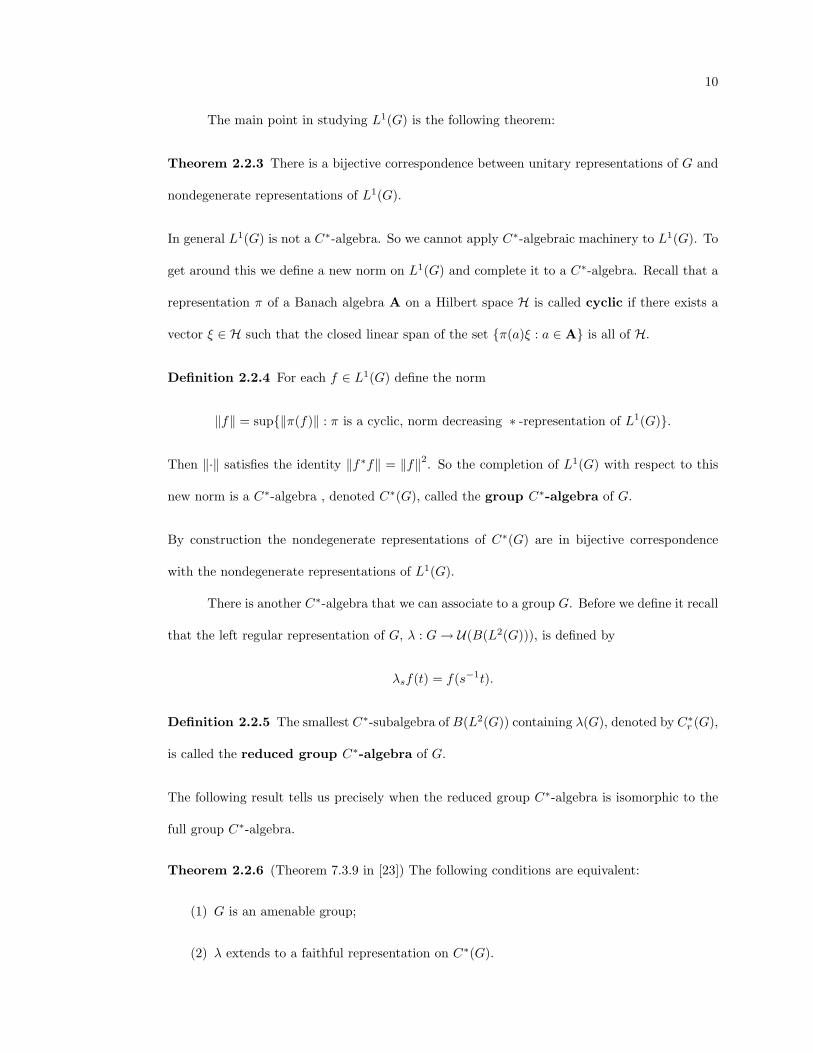
The main point in studying L1(G) is the following theorem:
Theorem 2.2.3 There is a bijective correspondence between unitary representations of G and
nondegenerate representations of L1(G).
In general L1(G) is not a C∗-algebra. So we cannot apply C∗-algebraic machinery to L1(G). To
get around this we define a new norm on L1(G) and complete it to a C∗-algebra. Recall that a
representation π of a Banach algebra A on a Hilbert space H is called cyclic if there exists a
vector ξ ∈ H such that the closed linear span of the set π(a)ξ : a ∈ A is all of H.
Definition 2.2.4 For each f ∈ L1(G) define the norm
‖f‖ = sup‖π(f)‖ : π is a cyclic, norm decreasing ∗ -representation of L1(G).
Then ‖·‖ satisfies the identity ‖f∗f‖ = ‖f‖2. So the completion of L1(G) with respect to this
new norm is a C∗-algebra , denoted C∗(G), called the group C∗-algebra of G.
By construction the nondegenerate representations of C∗(G) are in bijective correspondence
with the nondegenerate representations of L1(G).
There is another C∗-algebra that we can associate to a group G. Before we define it recall
that the left regular representation of G, λ : G→ U(B(L2(G))), is defined by
λsf(t) = f(s−1t).
Definition 2.2.5 The smallest C∗-subalgebra of B(L2(G)) containing λ(G), denoted by C∗r (G),
is called the reduced group C∗-algebra of G.
The following result tells us precisely when the reduced group C∗-algebra is isomorphic to the
full group C∗-algebra.
Theorem 2.2.6 (Theorem 7.3.9 in [23]) The following conditions are equivalent:
(1) G is an amenable group;
(2) λ extends to a faithful representation on C∗(G).
11
Since all the groups we will be dealing with are finite extensions of abelian groups, they are all
amenable. So we will use C∗(G) and C∗r (G) interchangeably. Moreover, since amenability of a
discrete group G is equivalent to C∗r (G) being nuclear [23] and all other C∗-algebras we see will
be nuclear, we will use ⊗ to denote the unique tensor product of C∗-algebras.
2.3 C∗-bundles
A very useful result for later computations will be the realization of certain C∗-algebras as
section algebras of certain fibre bundles over CW -complexes with finite dimensional C∗-algebras
as fibres. The following definitions and theorems are from [8].
Definition 2.3.1 A Banach bundle is a bundle ξ = (p,E,X) such that
(1) for each x ∈ X, Ex is a Banach space
(2) (a) for each λ ∈ C, the map x 7→ λx is a continuous map from E to E
(b) vector addition is continuous as a function on (x, y) ∈ E × E : p(x) = p(y)
(c) the map x 7→ ‖x‖ is continuous from E to R.
(3) if 0x ∈ W , where 0x denotes the zero element in Ex and W is open in E, then there is
an ε > 0 and an open neighborhood U ⊆ X of x such that b ∈ p−1(U) : ‖b‖ < ε ⊆W .
Definition 2.3.2 A C∗-bundle is a Banach bundle ξ = (p,E,X) where each fibre Ex is a
C∗-algebra such that
(1) multiplication is a continuous as a function on (x, y) ∈ E × E : p(x) = p(y)
(2) the involution is continuous on E.
If X is a locally compact space and ξ = (p,E,X) is a C∗-bundle , then Γ0(ξ), equipped
with pointwise multiplication and involution, and the supremum norm, is a C∗-algebra.
Example 2.3.3 If X is locally compact, then C0(X) is the section algebra of the trivial bundle
C×X over X.

12
It should be noted that we have made no assumption about local triviality of the above
defined bundles. In fact, the bundles that we will be concerned with are decidedly not locally
trivial. The advantage of dropping the assumption of local triviality is the widespread application
of non-locally trivial C∗-bundles , expressed in the following version of Corollary 8.13 from [6],
found in [8].
Theorem 2.3.4 If B is a C∗-algebra and A is a C∗-subalgebra of the center ofM(B) containing
an identity for M(B), and if X = A, then there is a ∗-isomorphism ˜ : B → Γ(ξB) of B onto
the C∗-algebra of all sections of a C∗-bundle ξB. Moreover, every irreducible representation of
Γ(ξB) factors through a point evaluation.
2.4 K-theory of C∗-algebras
This section is taken from [29]. Let A be a unital C∗-algebra. First we define a semigroup
out of the projections in A. Let Pn(A) = P(Mn(A)) be the set of all projections in Mn(A).
Then let P∞(A) = ∪nPn(A). The reason for taking matrices is to allow us to take sums: for
p ∈ Pn(A), q ∈ Pm(A) the sum p ⊕ q = diag(p, q) ∈ Pn+m(A). Now define an equivalence
relation ∼0 on P∞(A) by saying p ∼0 q if there exists a partial isometry v ∈ Mm,n(A), the
m× n matrices over A, such that p = v∗v and q = vv∗. Let D(A) = P∞(A)/ ∼0. Then under
the operation [p]0 + [q]0 = [p⊕ q]0 D(A) is an abelian semigroup.
For any abelian semigroupD there is an abelian groupG(D) defined asG(D) = D×D/ ∼,
where (a, b) ∼ (c, d) if and only if a+ d = c+ b. This group is called the Grothendieck group
of D.
Definition 2.4.1 If A is a unital C∗-algebra, define K0(A) = G(D(A)).
Definition 2.4.2 Suppose A is a C∗-algebra without unit. For each a ∈ A define La to be the
linear operator from A to A defined by La(b) = ab. Let A1 be the set of all operators from
A to A of the form λ1 + La for λ ∈ C and a ∈ A. Then A1 is a unital C∗-algebra under the
13
operator norm and involution (λ1+La)∗ = λ1+La∗ . Moreover, A1 contains A as a closed ideal
of codimansion 1. A1 is called the unitification of A.
Definition 2.4.3 If A is a nonunital C∗-algebra , K0(A) is defined to be the kernel of the
homomorphism K0(π) where π is the quotient morphism A1 → C.
Theorem 2.4.4 K0 is a covariant functor from the category of all C∗-algebras into the category
of abelian groups. Moreover, K0 is stable in that K0(Mn(A)) = K0(A).
We now turn our attention to K1 of a C∗-algebra A. Let Un(A1) denote the group of all
unitary elements in Mn(A1). Then let U∞(A1) = ∪nUn(A1). Define a binary operation ⊕ on
U∞(A1) by u ⊕ v = diag(u, v). Then define an equivalence relation ∼1 on U∞(A1) by saying
u ∈ Un(A1) is equivalent to v ∈ Um(A1) if there is a k ≥ maxn,m such that
u⊕ 1k−n ∼h v ⊕ 1k−m
where ∼h denotes homotopy equivalence, i.e. there is a continuous path of unitaries ut : [0, 1] →
Uk(A) such that u0 = u ⊕ 1k−n and u1 = u ⊕ 1k−m. Then it turns out that U∞(A)/ ∼1 is an
abelian group, so we make the following definition.
Definition 2.4.5 Let A be a C∗-algebra. Then define K1(A) = U∞(A1)/ ∼1.
Theorem 2.4.6 K1 is a stable covariant functor from the category of all C∗-algebras into the
category of abelian groups.
Example 2.4.7 The following is a table of K groups that we will need to know. It is part of
the very useful table found in [29].
Here SA = C0((0, 1),A) is known as the suspension of A. Some of the entries in this table are
much harder to prove than others. For instance, the bottom row is the very deep fact known as
Bott periodicity. Since we will never use the isomorphism involved in Bott periodicity explicitly,
all we need to know is that it exists and allows us to regard K∗ as a Z2-graded generalized

14C∗-algebra K0 K1
Mn(C) Z 0C([0, 1]n) Z 0
C0((0, 1)n) n-odd 0 ZC(Sn) n-even Z⊕ Z 0C(Sn) n-odd Z ZMn(A) K0(A) K1(A)A⊕B K0(A)⊕K0(B) K1(A)⊕K1(B)SA K1(A) K0(A)
Table 2.1: some important K groups
homology theory on the category of C∗-algebras by defining Kn(A) = K0(SnA). The row
regarding Sn, when n is odd is worthy of some remarks for later computations.
First we would like to show that the class [1]0 generates K0(C(S1)). To achieve this we
will need the following result:
Proposition 2.4.8 If
0 I A B 0................................................................................................................. ............ ................................................................................................................. ............ ................................................................................................................. ............π
............................................................................................................................. σ................................................................................................................. ............
is a split exact sequence of C∗-algebras , then
0 K0(I) K0(A) K0(B) 0........................................................................................ ............ ............................................................... ............ ............................................................... ............[π]0
...........................................................................
[σ]0................................................................................................................. ............
is a split exact sequence of abelian groups.
To get the desired result we note that in the proof that K0(C(S1)) = Z, one simply uses
the split exactness of K0 and the fact that the extension
0 C0(0, 1) C(S1) C 0........................................................................................ ............ ........................................................................... ............ ........................................................................................ ............ ................................................................................................................. ............
is split by taking z ∈ C to z1 ∈ C(S1). The second thing to note is that the isomorphism
between K1(C(S1)) and Z is given by taking a unitary u ∈ C(S1) to its winding number. Both
of these observations are critical to the computations carried out in Chapter 5.
Finally we end this section with one of the main results in K-theory.

15
Theorem 2.4.9 (12.1.2 in [29]) For every short exact sequence of C∗-algebras
0 I A B 0................................................................................................................. ............ ................................................................................................................. ............
ϕ................................................................................................................. ............
π......................... ............ ................................................................................................................. ............
there is an associated six-term exact sequence
K0(I) K0(A) K0(B).......................................................................................................................................... ............[ϕ]0
................................................................................................................. ............[π]0
K1(I)K1(A)K1(B) ......................................................................................................................................................
[ϕ]1.............................................................................................................................
[π]1
........
........
........
........
........
........
........
........
........
........
........
........
.................
............
∂1
.............................................................................................................................
∂0
It is useful to know that the six-term exact sequence is natural in the sense that if the diagram
0 I A B 0................................................................................................................. ............ ................................................................................................................. ............
ϕ................................................................................................................. ............π′ ................................................................................................................. ............
0 I′ A′ B′ 0................................................................................................................. ............ .................................................................................................... ............
ϕ′........................................................................................ ............π′ ................................................................................................................. ............
.............................................................................................................................
γ
.............................................................................................................................
α
.............................................................................................................................
λ
is commutative and the rows are extensions with associated six-term exact sequences
K0(I) K0(A) K0(B).......................................................................................................................................... ............[ϕ]0
................................................................................................................. ............[π]0
K1(I)K1(A)K1(B) ......................................................................................................................................................
[ϕ]1.............................................................................................................................
[π]1
........
........
........
........
........
........
........
........
........
........
........
........
.................
............
∂1
.............................................................................................................................
∂0
and
K0(I′) K0(A′) K0(B′).......................................................................................................................................... ............[ϕ′]0
................................................................................................................. ............[π′]0
K1(I′)K1(A′)K1(B′) ......................................................................................................................................................
[ϕ′]1.............................................................................................................................
[π′]1
........
........
........
........
........
........
........
........
........
........
........
........
.................
............
∂′1
.............................................................................................................................
∂′0
then the following diagrams commute:
K1(B) K0(I)
K1(B′) K0(I′)
.................................................................................................. ............∂1
..............................................................................................................
[λ]1
.................................................................................................. ............∂′1
..............................................................................................................
[γ]0

16K0(B) K1(I)
K0(B′) K1(I′)
.................................................................................................. ............∂0
..............................................................................................................
[λ]0
.................................................................................................. ............∂′0
..............................................................................................................
[γ]1
.
2.5 Hilbert C∗-modules and Morita equivalence
Here we will collect some basic facts about Hilbert C∗-modules and Morita equivalence.
The main purpose will be to define Morita equivalence and present the most essential facts:
Morita equivalent C∗-algebras have essentially the same representation theory and K-theory is
a Morita invariant. Along the way we will use a particular Hilbert C∗-module to give an explicit
construction of the multiplier algebra of a C∗-algebra.
Definition 2.5.1 Let A be a C∗-algebra. A right A-module XA is called an right inner
product A-module if there exists a pairing 〈 , 〉A : X×X → A with the following properties:
(1) 〈x, y + z〉A = 〈x, y〉A + 〈x, z〉A
(2) 〈x, y · a〉A = 〈x, y〉Aa
(3) 〈x, y〉∗A = 〈y, x〉A
(4) 〈x, x〉A ≥ 0 as elements of A
(5) 〈x, x〉A = 0 if and only if x = 0.
Definition 2.5.2 Let A be a C∗-algebra. A left A-module XA is called an left inner product
A-module if there exists a pairing A〈 , 〉 : X ×X → A with the following properties:
(1) A〈x, y + z〉 = A〈x, y〉+ A〈x, z〉
(2) A〈a · x, y〉 = aA〈x, y〉
(3) A〈x, y〉∗ = A〈y, x〉
(4) A〈x, x〉 ≥ 0 as elements of A.

17
(5) A〈x, x〉 = 0 if and only if x = 0.
Definition 2.5.3 BXA is an inner product B-A-bimodule if it is simultaneously a left
inner product B-module and a right inner product A-module.
We will often want a norm on our modules, which leads to the following proposition:
Proposition 2.5.4 (Corollary 2.7 in [26]) If XA is an inner product A-module, then
‖x‖X = ‖〈x, x〉A‖12
defines a norm on X. The same holds true for left modules with the obvious modification.
Definition 2.5.5 An inner product A-module is called a Hilbert A-module if it is complete
in the above norm.
It should be noted, for the purpose of doing computations, that if XA is a right Hilbert A-
module, the inner product is conjugate linear in the first variable and linear in the second. For
left modules it is the opposite. Then we can see that Hilbert spaces are left Hilbert C-modules.
Example 2.5.6 If A is a C∗-algebra, then it is natural to let A act on itself on the right, thus
making it into a right A module AA. It is easy to check that when we set 〈a, b〉A = a∗b, AA
becomes a right Hilbert A-module. One can also make A into a left Hilbert A-module by letting
A act on itself on the left, and letting the inner product be A〈a, b〉 = ab∗. We then call it AA.
We will see more examples of Hilbert C∗-modules as they are needed.
Definition 2.5.7 A (right) Hilbert A-module X is called full if span 〈x, y〉A : x, y ∈ X is
dense in A.
Example 2.5.8 The above examples are clearly full.
For defining Morita equivalence we will need to discuss operators on Hilbert C∗-modules.

18
Definition 2.5.9 Suppose X and Y are Hilbert C∗-modules over a C∗-algebra A. A module
homomorphism T : X → Y is called an adjointable operator if there exists T ∗ : Y → X such
that for x ∈ X and y ∈ Y , 〈Tx, y〉A = 〈x, T ∗y〉A.
Lemma 2.5.10 [26] Adjointable operators on Hilbert C∗-modules are bounded in the operator
norm.
For left Hilbert C-modules, i.e. Hilbert spaces, all bounded operators are adjointable. However,
the converse to the above Lemma is not true. There are bounded operators between Hilbert
C∗-modules that are not adjointable. The way we get around this is by only studying the
operators that are adjointable in the way that we study B(H). To this end we make the
following definitions:
Definition 2.5.11 The set of all adjointable operators from X to Y is denoted by L(X,Y ).
When X = Y , we will write L(X).
Definition 2.5.12 Let θy,x : X → Y denote the rank one operator defined by θy,x(w) =
y〈x,w〉A. The norm closure of span θy,x : y ∈ Y, x ∈ X is called the set of A-compact oper-
ators from X to Y . It is denoted by K(X,Y ) or just K(X) if X = Y .
Obviously these definitions were made to coincide with the analogous definitions for
regular Hilbert spaces when A = C. The structure works out in much the same way.
Theorem 2.5.13 [14] For a C∗-module X over a C∗-algebra A, L(X) and K(X) are C∗-
algebras . Moreover, K(X) is an essential ideal in L(X).
Definition 2.5.14 For a C∗-algebra A, the multiplier algebra M(A) is the largest C∗-
algebra containing A as an essential ideal in the following sense. Suppose j : A → B is an
inclusion of A as an ideal in B. Then there is a unique map θ : B →M(A) so that
A
M(A)
B.............................................................................................................................
ι
................................................................................................................. ............j ...........
......................
......................
......................
......................
......................
......................
.........................................
θ
19
commutes. Moreover, if j(A) is essential in B, θ is injective.
Example 2.5.15 If A is a C∗-algebra , then A ∼= K(AA) and M(A) ∼= L(AA) [26].
Before moving on to Morita equivalence we should say one more thing. It turns out that
a Hilbert space is finite dimensional whenever the identity is compact. This fact essentially
extends to Hilbert C∗-modules over unital C∗-algebras .
Proposition 2.5.16 (Proposition 3.9 in [14]) A right C∗-module X over a unital C∗-algebra
A is finitely generated and projective if and only if the identity operator 1X is compact.
Now we can make the fundamental definition for Morita equivalence.
Definition 2.5.17 Let A and B be C∗-algebras . Define a B-A equivalence bimodule to
be a B-A bimodule BXA such that
(1) BXA is full as both a right A-module and as a left B-module
(2) For all a ∈ A and b ∈ B, 〈bx, y〉A = 〈x, b∗y〉A and B〈xa, y〉 = B〈x, ya∗〉.
(3) For all x, y, z ∈ BXA, B〈x, y〉z = x〈y, z〉A.
Definition 2.5.18 Two C∗-algebras A and B are said to be Morita equivalent if there exists
a B-A equivalence bimodule. We denote this by A ∼m B.
Example 2.5.19 Let A be any C∗-algebra . Then the set of n dimensional column vectors
An has an obvious structure as a right A-module and as a left Mn(A)-module. For a,b ∈
An we can define two inner products Mn(A)〈a,b〉 = a(b∗)T and 〈a,b〉A = a∗b. Elementary
computations show that, with these inner products, An is an Mn(A)-A-imprimitivity bimodule,
so A ∼m Mn(A).
It is the previous example and 2.5.16 which are essentially used in proving the following
theorem in [28]. It is important in that it gives a way to explicitly write down elements of im-
primitivity modules in the case when both C∗-algebras are unital. Note that if A is a subalgebra
20
of B, then A is a corner if there is some projection p ∈ B such that A = pBp. A is a full corner
if it is contained in no nontrivial, closed, two sided ideal in B.
Theorem 2.5.20 If A and B are unital C∗-algebras that are Morita equivalent, then A is
isomorphic to a full corner of the algebra of n × n matrices over B for suitable n and B is
isomorphic to a full corner of the algebra of m×m matrices over A for suitable m.
Theorem 2.5.21 If A ∼m B, where A and B are unital C∗-algebras, then K∗(A) ∼= K∗(B).
Proof. See [28].
2.6 Crossed Products, Twisted and Untwisted
Two of the main results in this thesis concern certain crossed product C∗-algebras . Here
we will define crossed product C∗-algebras, both untwisted and twisted, and consider some
particularly nice examples.
Definition 2.6.1 (Def 2.1 in [22]) Suppose A is a separable C∗-algebra and G a countable
discrete group. A twisted action of G on A is a pair of maps α : G → Aut(A) and u :
G×G→ UM(A) such that
(1) u is strictly Borel and for each a ∈ A, s 7→ αs(a) is Borel,
(2) αe = id, u(s, e) = u(e, s) = 1 for all s ∈ G,
(3) αs αt = Adu(s, t) αst for s, t ∈ G,
(4) αr(u(s, t))u(r, st) = u(r, s)u(rs, t) for r, s, t ∈ G.
The quadruple (A, G, α, u) is called a twisted C∗-dynamical system.
Remark 2.6.2 For the general case, where the groups are not assumed to be discrete, see [22].
Now let (A, G, α, u) be a twisted C∗-dynamical system. Let Cc(G,A, α, u) denote the
linear space of continuous functions from G to A with compact support. On this space define

21
the convolution and involution as follows:
(f ? g)(x) =∑y∈G
f(y)[αy[g(y−1x)]u(y, y−1x)] and f∗(x) = u(x, x−1)∗[αxf(x−1)∗].
It is shown in [4] that these operations make Cc(G,A, α, u) into a complex ∗-algebra. Let
L1(G,A, α, u) denote the completion of Cc(G,A, α, u) under the norm
‖f‖1 =∑y∈G
‖f(y)‖ .
Now L1(G,A, α, u) is a Banach ∗-algebra. When the system is untwisted, that is, when u = 1,
we will just write Cc(G,A) and L1(G,A).
Definition 2.6.3 A covariant representation of a twisted C∗-dynamical system (A,G, α, u)
is a pair (π,U) consisting of a nondegenerate representation π of A on a separable Hilbert space
H and a map U : G→ U(H) such that
(1) UsUt = π(u(s, t))Ust
(2) π(αs(a)) = Ad(Us)(π(a)).
Definition 2.6.4 Let S be a set of cyclic covariant representations of (A,G, α, u) such that
every cyclic covariant representation of (A,G, α, u) is equivalent to a member of S. Let H =
⊕Hπ,U : (π,U) ∈ S and define the twisted crossed product A oα,u G to be the norm
closure of the set span(⊕π(a))(⊕U(f)) ⊂ B(H) where a ∈ A and f ∈ L1(G).
The point of the above definition is that A oα,u G is the universal C∗-algebra for covariant
representations of (A,G, α, u) and thus representations of L1(G,A, α, u): i.e. the C∗-algebra
generated by any covariant representation of (A,G, α, u) is the image of a representation of
A oα,u G. When we consider Cc(G,A, α, u) an explicit formula can be obtained. Let S be as
above. Then for each (π,U) ∈ S define a representation π o U of Cc(G,A) by
π o U(f) =∑s∈G
π(f(s))Us.

22
Then π o U extends to a representation of L1(G,A) and thus a representation of A oα G. We
will regularly use the correspondence of representations π o U and covariant representations of
(A, G, α).
Example 2.6.5 When the action of a group G on a C∗-algebra A is trivial and untwisted then
covariant representations of (A, G, α) are in bijective correspondence with commuting pairs
(π,U) of representations of A and G respectively. Then, by the respective universal properties
of the group C∗-algebra C∗(G) and the tensor product, we have A oα G ∼= A⊗C∗(G).
Example 2.6.6 When G is a extension of an abelian group N , and D = G/N , then C∗(G) =
C∗(N) o D. Take a section s of the map π : G → G/N such that s(d) ∈ d for all d ∈ D and
s(eD) = eG. Then there is a well defined action of D on N given by d ·n = s(d)ns(d)−1. There is
also an induced action of D on N given by d ·χ(n) = χ(d−1 ·n). Hence we obtain an action of D
on C∗(N) = C(N) by αdf(χ) = f(d−1 ·χ). Therefore the map u will come from the two-cocycle
σ : D × D → N such that s(a)s(b) = s(ab)σ(a, b), which determines the isomorphism class of
the extension given the conjugation action of D on N . Simply define u(a, b)(χ) = χ(σ(a, b)).
The only condition that is not obvious is (4) in the definition of a twisted C∗-dynamical system.
However, using the cocycle identity r · σ(s, t)σ(r, st) = σ(r, s)σ(rs, t) we obtain
αr(u(s, t))(u(r, st))(χ) = u(s, t)(r−1 · χ)u(r, st)(χ)
= χ(r · σ(s, t))χ(u(r, st))
= χ(r · σ(s, t)u(r, st))
= χ(σ(r, s)σ(rs, t))
= χ(σ(r, s))χ(σ(r, st))
= (u(r, s)u(rs, t))(χ).
Thus (C0(N), D, α, u) is a twisted C∗-dynamical system. It follows from [15] that C∗(G) ∼=
C(N) oα,u D.
23
When G is finite we can write the crossed product by G very explicitly by using the
following result due to Rieffel [27]. Recall that if U is a unitary element in a C∗-algebra, then
AdU : A → A denotes the automorphism a 7→ UaU∗.
Theorem 2.6.7 Let (A, G, α) be a C∗-dynamical system with G compact. Then A oα G is
naturally isomorphic to the fixed point algebra of A⊗K(L2(G)) under the action α⊗Adρ where
ρ is the right regular representation of G on L2(G) defined by ρg(f)(t) = f(tg).

Chapter 3
NCCW -Complexes
3.1 Definitions and Basic Properties
In this section we will recall some definitions from [9], [10], and [24], as well as some
important facts. We will begin by setting some notation, borrowed directly from Pedersen’s
paper[24]. If A is a C∗-algebra , then
InA = C([0, 1]n,A), In0A = C0((0, 1)n,A), SnA = C(Sn,A)
where we identify the n-sphere Sn with the boundary of [0, 1]n+1.
Definition 3.1.1 A zero dimensional noncommutative CW -complex (NCCW -complex)
is any finite dimensional C∗-algebra A0, as described in 1.1.7. In general we recursively define
an n-dimensional NCCW -complex to be any C∗-algebra An appearing in a diagram
0 In0Fn An An−1 0.................................................................................................... ............ ................................................................................................................. ............ .................................................................................................... ............
πn .................................................................................................... ............
0 In0Fn InFn Sn−1Fn 0.................................................................................................... ............ .................................................................................................... ............ ........................................................................... ............δ .................................................................................................... ............
.....................................................................................................
.....................................................................................................
.............................................................................................................................
fn
.............................................................................................................................
ϕn
where the rows are extensions and the right hand square is a pullback. Here An−1 denotes
an (n − 1)-dimensional NCCW -complex, Fn is some finite dimensional C∗-algebra , δ is the
boundary restriction map, and ϕn is an arbitrary morphism called the connecting morphism.

25
The maps fn and πn are the projections onto the first and second coordinates, respectively, in
the realization of An as a restricted direct sum
An = InFn
⊕Sn−1Fn
An−1.
Any NCCW -complex An of dimension n ≥ 1 will be assumed to have lower dimensional com-
plexes Ak with k < n such that Ak−1 is the image under the projection πk appearing in the
diagram making Ak a k-dimensional NCCW -complex.
Example 3.1.2 Recall from [12] that a space X is a finite, n-dimensional CW -complex if there
is a filtration X0 ⊆ X1 ⊆ · · · ⊆ Xn = X such that X0 is a finite discrete space, and for
k = 1, . . . , n, Xk arises in the pushout diagram
Xk Xk−1
⊔λk
Ik⊔λk
Sk−1
..............................................................................................................
........
........
........
........
........
........
........
........
........
........
..................
............
.............................................................................................................. ι
........
........
........
........
........
........
........
........
........
........
..................
............
γk
.
Here λk denotes some finite index set, Ik = [0, 1]k, the horizontal maps are the the obvious
inclusions, and γk is an arbitrary continuous map. By dualizing this diagram we obtain a
pullbackC(Xk) C(Xk−1)
IkCλk SkCλk
.................................................................................................. ............πk
..............................................................................................................
.................................................................................................. ............ι∗ = δ
..............................................................................................................
γ∗k = ϕk
.
This makes C(X) into a (commutative!) NCCW -complex.
The fact that, in the definition of an NCCW -complex, there is no restriction made on
the connecting morphisms is worthy of some remarks. In the previous example, it is possible
that the k-skeleton is equal to the (k− 1)-skeleton. This occurs when the index set λk is empty.
In the general situation this corresponds to the finite dimensional C∗-algebra Fk appearing in
the diagram with IkFk being equal to zero. In this case, we could also write Ak as a (k − 1)-

26
dimensional NCCW -complex. Occasionally we will need to assume this does not happen, so we
will make the following definition:
Definition 3.1.3 Suppose n ≥ 1 and An is an n-dimensional NCCW -complex with lower
dimensional complexes A0, · · ·An−1. An is called strongly n-dimensional if all the connecting
morphisms ϕk : Ak−1 → Sk−1Fk are nonzero. A CW -complex X is strongly n-dimensional if
C(X) is a strongly n-dimensional NCCW -complex when it us decomposed as in the previous
example.
If A1 is a strongly one-dimensional NCCW -complex then the finite dimensional algebras
A0 and F1 must be unital. Then A1 is unital if and only if ϕ1 is a unital morphism. In general,
if An is a strongly n-dimensional NCCW -complex, An is unital if and only if An−1 is unital
and that the connecting morphism ϕn is unital. This is due to the fact that the only unit in
InFn for the ideal In0Fn ⊂ InFn is the unit 1 ∈ InFn. It follows that all the lower dimensional
complexes Ak and their corresponding connecting morphisms ϕk are unital. In practice, all our
NCCW -complexes will be unital, so we will assume they are from now on. This is really a
very small restriction to make (see section 11.2 in [24]). Moreover we will assume that nonzero
morphisms between nonzero finite dimensional C∗-algebras are unital.
Another possibility in a commutative CW -complex is that some parts of a given CW -
complex appear to have lower dimension than the rest of the complex. For instance, take the
disjoint union of a closed disk and a closed interval. In the noncommutative case this corresponds
to a connecting morphism not being injective. So from [24] we recall the following definition.
Definition 3.1.4 An n-dimensional NCCW -complex is called proper if all the connecting
morphisms appearing in its construction are injective. This occurs if and only if the ideals Ik0Fk
are essential in Ak.
Definition 3.1.5 Suppose An is an n-dimensional NCCW -complex. Define the canonical
ideals in An to be the decreasing family of closed ideals
An = I0 ⊃ I1 ⊃ · · · ⊃ In 6= 0

27
by setting Ik equal to the kernel of the composition
Anπn→ An−1
πn−1→ · · · πk→ Ak−1.
So we have In = In0Fn, An/Ik+1
∼= Ak, and Ik/Ik+1∼= Ik
0Fk. For the purpose of consistency,
we will let Ik = 0 for k > n.
Example 3.1.6 To make the previous definition more concrete, let X be a finite, n-dimensional
CW -complex containing cells of each dimension ≤ n. Then as in the previous example we have
a decomposition of C(X) as an n-dimensional NCCW -complex, with Ak = C(Xk) where Xk
denotes the k-skeleton of X. Then Ik = C0(X \Xk−1) and Ik/Ik+1∼= Ik
0Cλk , where λk denotes
the number of open k-cells.
Example 3.1.7 Let A = f ∈ C([0, 1],M2(C)); f(0)andf(1)are diagonal . Then we can de-
compose A as a one-dimensional NCCW -complex in the following way: let A0 = C4, F1 =
M2(C) and define the connecting morphism ϕ1 : A0 → F21 by
ϕ1(a, b, c, d) =
a 0
0 b
,
c 0
0 d
.
Then we have the canonical ideals I0 = A and I1 = I10M2(C).
Remark 3.1.8 Suppose An is strongly n-dimensional. Then there is a particularly nice way
of writing elements of the algebra and of the canonical ideals. Suppose the lower dimensional
complexes are of the form Ak = IkFk
⊕Sk−1Fk
Ak−1, then we may write An as an iterated
restricted direct sum
An = InFn
⊕Sn−1Fn
In−1Fn−1
⊕Sn−2Fn−1
· · ·⊕F2
1
A0.
Then we may regard elements of An as (n + 1)-tuples (an, . . . , a0), where ak ∈ IkFk for k > 0
and a0 ∈ A0, such that δ(ak) = ϕk((ak−1, . . . , a0)) in Sk−1Fk for 1 ≤ k ≤ n. Then the canonical
ideals have the form
Ik = (an, an−1, . . . , ak, 0, . . . , 0) ∈ An : ak ∈ Ik0Fk.

28
Then the quotients become very transparent.
The following, from [24], generalizes the notion of a cellular map of CW -complexes. They
will be used decisively in the next section to make the action of a finite group on an NCCW -
complex compatible with the cellular decomposition.
Definition 3.1.9 Suppose
A = InFn
⊕Sn−1Fn
In−1Fn−1
⊕Sn−2Fn−1
· · ·⊕F2
1
A0
and
B = ImGm
⊕Sm−1Gm
Im−1Gm−1
⊕Sm−2Gm−1
· · ·⊕G2
1
B0
are NCCW -complexes of dimensions n and m, with canonical ideals Iknk=0 and Jkm
k=0,
respectively. For 0 ≤ k ≤ n, let Ik/Ik+1 = Ik0Fk and Jk/Jk+1 = Ik
0Gk. A morphism α : A → B
is called simplicial if
(1) α(Ik) ⊆ Jk
(2) Then by condition (1) there is an induced morphism αk : Ik0Fk → Ik
0Gk. Then there
exists a morphism ψk : Fk → Gk and a homeomorphism ιk of Ik such that αk = ι∗k⊗ψk,
where ι∗k denotes the dualized version of ιk.
When A is an NCCW -complex and α is a simplicial automorphism of A, it is assumed
that α is simplicial for a fixed decomposition of A. That is, the decomposition is the same when
viewing A as the domain or the codomain of α. If one considers the A = C[0, 1] decomposed
as an NCCW -complex with one 1-cell and two 0-cells for the domain of the identity morphism,
and with two one-cells and three 0-cells for the codomain, then the identity is not simplicial.
This is obviously corrected by giving A the same, finer, decomposition on both ends.
It should also be noted that whenever speaking of simplicial morphisms between NCCW -
complexes An and Bm we may take n = m [24]. To see this all we have to do is take pullbacks

29
over the zero algebra to make the dimensions match up. So if m > n, we define
Ak = Ik0⊕
Sk−10
Ak−1 , n+ 1 ≤ k ≤ m.
In this case a simplicial morphism clearly remains simplicial as all the higher homogeneous
algebras and ideals are 0. We would define the higher dimensional Bk similarly if n > m. In
this case we cannot assume that An or Bm are strongly n or m dimensional. In practice, i.e.
with group actions, it is most often the case that n = m anyway, without ever having to take
pullbacks over 0.
3.2 Crossed Products of NCCW -Complexes
Proposition 3.2.1 Suppose An and Bn are strongly n-dimensional (n ≥ 1)NCCW -complexes,
with decompositions as in 3.1.9, and α : An → Bn is a simplicial morphism. Then αn−1(a +
In) = α(a) + Jn defines a simplicial morphism αn−1 : An−1 → Bn−1 and α is the unique
∗-homomorphism making the following diagram commute:
In0Fn An An−1....................................................................................................................................................................................................................................................................... ............ .......................................................................................................................................................................................................................................................... ............
πn
In0Fn InFn Sn−1Fn
.......................................................................................................................................................................................................................................................... ............ ................................................................................................................................................................................................................................. ............δ
...........................................................................................................................................................................................................................................................
...........................................................................................................................................................................................................................................................
...................................................................................................................................................................................................................................................................................
...................................................
fn
...................................................................................................................................................................................................................................................................................
γn
In0Gn Bn Bn−1....................................................................................................................................................................................................................................................................... ............ .......................................................................................................................................................................................................................................................... ............
πn
In0Gn InGn Sn−1Gn
................................................................................................................. ................................................................................................................. ............ ................................................................................................................. ........................................................................... ............δ
.................................................................................................................
.................................................................................................................
.................................................................................................................
.................................................................................................................
.....................................................................................................
.........................................................................................................................................
gn
...................................................................................................................................................................................................................................................................................
σn
........................................................................................................................................................................................
ι∗n ⊗ ψn
........................................................................................................................................................................................
ι∗n ⊗ ψn
........................................................................................................................................................................................
α
........................................................................................................................................................................................
ι∗n ⊗ ψn
........................................................................................................................................................................................
αn−1
........................................................................................................................................................................................
ι∗n ⊗ ψn
where γn and σn are the respective connecting morphisms.
Proof. First we note that αn−1 is a well defined morphism because α(In) ⊆ Jn. To show that
αn−1 is simplicial, put An, Bn, An−1, and Bn−1 into their standard forms as in 3.1.8 and let
30
I ′kn−1k=0 and J ′k
n−1k=0 be the canonical ideals for An−1 and Bn−1, respectively. Then we have iso-
morphisms I ′k/I′k+1
∼= (Ik/In)/(Ik+1/In) ∼= Ik/Ik+1∼= Ik
0Fk and J ′k/J′k+1
∼= (Jk/Jn)/(Jk+1/Jn) ∼=
Jk/Jk+1∼= Ik
0Gk. Explicitly, for fk ∈ Ik0Fk and gk ∈ Ik
0Gk we have the compositions
fk 7→ (an−1, · · · , fk, · · · , 0)+I ′k+1 7→ (an, · · · , fk, · · · , 0+In)+(Ik+1/In) 7→ (an, · · · , fk, · · · , 0)+Ik+1 7→ fk
gk 7→ (bn−1, · · · , gk, · · · , 0)+J ′k+1 7→ (bn, · · · , gk, · · · , 0)+Jn+(Jk+1/Jn) 7→ (bn, · · · , gk, · · · , 0)+Jk+1 7→ gk
are both the identity id∗⊗ id. So we have that the induced morphism αn−1,k = (id∗⊗ id) αk
(id∗ ⊗ id), and thus αn−1 is simplicial.
To show that this diagram commutes we first note that the front and back commute
by assumption. Obviously the leftmost square commutes, and the bottom commutes because
any homeomorphism of In must preserve the boundary. The top right square commutes by the
definition of αn−1. The top left square commutes because α is simplicial. To show that the
middle square commutes, consider the approximate identity for ak = hk ⊗ I ∈ In0Gn, where
hk is an approximate identity for C0(0, 1)n such that hk = 1 on sets of the form [ 1k , 1 −1k ]n.
Since ιn is a homeomorphism, h′k = (ι∗n)−1(hk) ∈ In0Fn. Let a′k = h′k ⊗ I. Now suppose
(f, a) ∈ An. We know that the middle square commutes on the ideals In0Fn and In
0Gn. So we
have that ι∗ ⊗ ψn fn((a′k, 0)(f, a)) = gn α((a′k, 0)(f, a)) for all k. Now, for each x ∈ (0, 1)n
we can find a k so that ak(x)f(x) = f(x). Then we have that
ι∗⊗ψnfn((f, a))(x) = ι∗⊗ψnfn((a′k, 0)(f, a))(x) = gnα((a′k, 0)(f, a))(x) = gnα((f, a))(x).
This holds true for all x in a dense subset of [0, 1]n, so the middle square commutes.

31
We show that the rightmost square commutes by a diagram chase. Indeed, for a ∈ An
we have
σn(αn−1(a+ In)) = σn(αn−1(πn(a)))
= σn(πn(α(a)))
= δ(gn(α(a)))
= δ(ι∗n ⊗ ψn(fn(a)))
= ι∗n ⊗ ψn(δ(fn(a)))
= ι∗n ⊗ ψn(γn(πn(a)))
= ι∗n ⊗ ψn(γn(a+ In)).
So the right square commutes. The uniqueness of α follows from the universal property of B as
a pullback.
Now we are prepared to prove the main results on crossed products of NCCW -complexes
with the assumption that the action is simplicial.
Proposition 3.2.2 Suppose An is a strongly n-dimensionalNCCW -complex, andG is a locally
compact group. If (An, G, α) is a C∗-dynamical system with αg simplicial for all g ∈ G, then
there are C∗-dynamical systems (An−1, G, αn−1), (InFn, G, α), and (Sn−1Fn, G, α) such that
the diagram0 In
0Fn An An−1 0.................................................................................................... ............ ................................................................................................................. ............ .................................................................................................... ............πn .................................................................................................... ............
0 In0Fn InFn Sn−1Fn 0.................................................................................................... ............ .................................................................................................... ............ ........................................................................... ............δ .................................................................................................... ............
.....................................................................................................
.....................................................................................................
.............................................................................................................................
fn
.............................................................................................................................
ϕn
is G-equivariant.
Proof. If we define, for g ∈ G, (αn−1)g = (αg)n−1 and αg = αg to be the induced morphism
(ι∗n⊗ψn)g, from the fact that αg is simplicial, then we have our dynamical systems. Equivariance
of the pullback is obvious from 3.2.1.

32
Theorem 3.2.3 (6.3 in [24]) If we have a pullback of C∗-algebras
D B
A C
................................................................................................................. ............g2
.............................................................................................................................
g1
................................................................................................................. ............δ
.............................................................................................................................
ϕ
and (A, G, α), (B, G, β), and (C, G, γ) are C∗-dynamical systems such that δ and ϕ are G-
equivariant morphisms then there is a unique C∗-dynamical system (D, G, τ) such that DoτG ∼=
A oα G⊕
CoγG B oβ G.
Corollary 3.2.4 Suppose An is a strongly n-dimensional NCCW -complex, G is a locally com-
pact group, and that (An, G, α) is a C∗-dynamical system, with αg simplicial for all g ∈ G.
Then with the actions defined as in 3.2.2, we have
An oα G ∼= (InFn oα G)⊕
(Sn−1FnoαG)
(An−1 oα G).
Proof. This is a straightforward application of 3.2.2 and 3.2.3.
Before proceeding to define a class of C∗-dynamical systems that have NCCW -complexes
as crossed products we need the following useful lemma. Recall that if α and β are actions of
a group G on C∗-algebras A and B respectively, then α⊗ β is the action on A⊗B defined on
elementary tensors by (α⊗ β)g(a⊗ b) = αga⊗ βgb.
Lemma 3.2.5 Suppose A is a unital C∗-algebra , and (B, G, α) is a C∗-dynamical system
with B unital and G locally compact. Then, with ι denoting the trivial action of G on A,
(A⊗B) oι⊗α G is naturally isomorphic to A⊗(B oα G).
Proof. We begin by showing that both of the above C∗-algebras have the same universal
property. Let (π,U,H) be a covariant representation of (A⊗B, G, ι⊗α). Then as π is a nonde-
generate representation of A⊗B, there is a unique pair of representations (π1, π2) of A and B,
respectively, such that for all a ∈ A and b ∈ B
π(a⊗b) = π1(a)π2(b) = π2(b)π1(a).

33
Note that π2 is unital since it is nondegenerate. So then the covariance condition implies that
π((ι⊗α)s(a⊗1B)) = Usπ1(a)U∗s = π1(a).
So π1 commutes with both π2 and U , and thus commutes with the representation π2 oα U
of B oα G. So from (π,U,H) we obtained a commuting pair (π1, π2 oα U), which gives a
representation of A⊗(B oα G). This correspondence is 1-1 since the correspondence between π
and (π1, π2) was 1-1.
Conversely take (π′1, π′2 oα U
′) to be a commuting pair that give a nondegenerate rep-
resentation of A⊗(B oα G). If hλ is an approximate unit for Cc(G,B) then we have for each
a ∈ A and b ∈ B
π′1(a)π′2(b) = lim
λπ′1(a)π
′2(b)(π
′2 oα U
′)(hλ)
= limλπ′1(a)(π
′2 oα U
′)(bhλ)
= limλ
(π′2 oα U′)(bhλ)π′1(a)
= π′2(b)π′1(a).
Similarly we can show that π′1 commutes with U ′ by taking translates of hλ. So if we let
π′ denote the representation of A⊗B coming from (π′1, π′2), then we have obtained a unique
covariant representation (π′, U,H) of (A⊗B, G, ι⊗α). So the two C∗-algebras have the same
universal property and are isomorphic.
To show that the isomorphism is natural we must make the isomorphism explicit some-
how. The isomorphism given by matching the universal properties is nothing more than identi-
fying the universal representations of these two C∗-algebras . Since every C∗-algebra is naturally
isomorphic to its universal representation we are finished.
Definition 3.2.6 A noncommutative G-CW -complex (NCGCW -complex) is a C∗-dynamical
system (An, G, α) where An is a strongly n-dimensional NCCW -complex, G is a locally com-
pact group, and for all g ∈ G, αg is a simplicial morphism so that the induced morphism (αg)k
has the form id∗ ⊗ (ψk)g.
34
Theorem 3.2.7 Suppose G is a finite group and (An, G, α) is a NCGCW -complex. Then the
crossed product An oα G is an n-dimensional NCCW -complex.
Proof. We will proceed by induction on n. Clearly, when n = 0, we have our result as the
crossed product is again finite dimensional. Then, with the notation as in 3.2.2, we have that
An−1 oαn−1 G is an (n − 1)-dimensional NCCW -complex, by the induction hypothesis. So,
with the notation as in 3.2.2 and 3.2.4, we must show that the crossed products InFn oα G and
Sn−1Fn oα G are of the form InF′n and Sn−1F′n, respectively, for some finite dimensional C∗-
algebra F′n. This is true by a simple application of 3.2.5. By naturality the induced morphism
δ′ : InF′n → Sn−1F′n is indeed the boundary restriction morphism.
Corollary 3.2.8 (Lemma 11.13 in [24]) If An is a strongly n-dimensional NCCW -complex,
then so is An ⊗Mk(C).
Proof. It is clear from the definition that Akn is a strongly n-dimensional NCCW complex.
We can decompose it as InFkn
⊕Sn−1Fk
nAk
n−1, where the pullback is taken over the obvious
morphisms. For (ai)ki=1 ∈ Ak
n and j ∈ Zk define an action α of Zk on Akn by αj(ai) = a(i+j)modk.
Then (Akn, α,Zk) is a NCGCW -complex whose crossed product is An ⊗Mk(C).
Example 3.2.9 We know from 3.1.7 that the C∗-algebra
A = f ∈ C([0, 1],M2(C)); f(0)andf(1)are diagonal
is a one-dimensional NCCW -complex. It is also well known (for instance see II.2.β in [5]) that
this C∗-algebra is isomorphic to C∗r (G), where G is the infinite dihedral group, Z o Z2. From
2.6.6 we know that C∗r (G) ∼= C(T)oZ2, where the action of Z2 is the dual of the action g ·z = z
on T. Now, using 3.2.7, we can obtain an NCCW decomposition for A in a more algorithmic
way.
To do this we first begin by giving C(T) a decomposition as a NCCW -complex in the
manner seen in 3.1.2. First recall that a fundamental domain is an open set Ω ⊂ X such that
(1) g · Ω⋂
Ω = ∅ ∀g 6= e

35
(2)⋃
g∈G g · Ω = X.
The subset Ω = z ∈ T : Im(z) > 0 is a fundamental domain for the action of Z2 = e, g on
T. Then we will let the open 1-cells of T be the sets g · Ω. The 0-cells are then just 1 and −1.
Then we obtain a decomposition
C(T) = I1C2⊕C4
C2,
where the pullback is taken over the maps δ : I1C2 → C4 and γ : C2 → C4 defined by
δ(f1, f2) = (f1(0), f1(1), f2(0), f2(1)) and γ(z, w) = (z, w, z, w).
Then the action αg(f)(z) = f(z) induces the actions αg(f1, f2) = (f2, f1), αg(a, b, c, d) =
(c, d, a, b), and α0 g(z, w) = (z, w) on I1C2, C4 and C2, respectively. So this makes (C(T),Z2, α)
into a NCZ2CW -complex. Thus the crossed product is a one-dimensional NCCW -complex.
For the purpose of doing computation we should make the pullback explicit.
Generic elements of each of the crossed products are as follows:
C2 oα0 Z2 =
(a, b) (c, d)
(c, d) (a, b)
: a, b, c, d ∈ C
C4 oα Z2 =
(a1, b1, c1, d1) (a2, b2, c2, d2)
(c2, d2, a2, b2) (c1, d1, a1, b1)
: ai, bi, ci, di ∈ C
and
I1C2 oα Z2 =
(f1, f2) (g1, g2)
(g2, g1) (f2, f1)
: f1, f2, g1, g2 ∈ C([0, 1])
.
Then we can write the morphisms γ and δ.
γ
(a, b) (c, d)
(c, d) (a, b)
=
(a, b, a, b) (c, d, c, d)
(c, d, c, d) (a, b, a, b)
and
δ
(f1, f2) (g1, g2)
(g2, g1) (f2, f1)
=
(f1(0), f1(1), f2(0), f2(1)) (g1(0), g1(1), g2(0), g2(1))
(g2(0), g2(1), g1(0), g1(1)) (f2(0), f2(1), f1(0), f1(1))

36
Examining the above morphisms and C∗-algebras , we see that the pullback of the crossed
products is
A1∼=
f1 g1
g2 f2
∈ C([0, 1])⊗M2(C) : f1(0) = f2(0), f1(1) = f2(1), g1(0) = g2(0), g1(1) = g2(1)
This is isomorphic to what we wanted, since we can simultaneously diagonalize over the end-
points of [0, 1]. If we do the diagonalization earlier in the process we would obtain the same
decomposition as 3.1.7.
The techniques of this example apply more generally to the case when a finite group acts
on a finite CW -complex by permuting the cells in each dimension. The decomposition in the
next theorem is particularly useful in computing the K-theory of certain group C∗-algebras and
crossed products arising from orbifolds.
Theorem 3.2.10 Suppose X is a finite, CW -complex, with skeletal filtration X0 ( X1 ( · · · (
Xn = X and G is a finite group. Moreover, assume G acts on X in such a way that the following
conditions hold:
(1) Whenever e is a k-cell of X, so is g · e for 0 ≤ k ≤ n and all g ∈ G
(2) If g · e = e, then g|e = ide
(in particular X is a G-CW -complex). Then C(X) o G is a strongly n-dimensional NCCW -
complex.
Proof. Let Ωk denote the collection of all open k-cells in X. Since G acts on Ωk by permutations
Ωk is partitioned by the orbits under the action of G. Let ΩkG = e1, . . . , ejk
be a cross section
of the G action on Ωk. Then we see that for each closed k-cell in e ∈ X, there is a unique
k-cell ej ∈ ΩkG such that e = g · ej for some g ∈ G. Also, for each e ∈ Ωk there is a continuous
surjection ψe : [0, 1]k → e. Then we have a surjection g · ψej : [0, 1]k → e. Also, by condition
(2), if h ∈ G is such that h ·ψej ([0, 1]k) = e, then h ·ψej = g ·ψej since (g−1 ·h)|ej = idej implies
that h = gs for some s in the stabilizer of ej under the action of G.

37
Let lk denote the number of k-cells for each k, and let Fk = Clk . For each f ∈ C(Xk)
and k-cell e ∈ Ωk, f |e ∈ C(e) and there is an injection (g · ψej)∗ : C(e) → C([0, 1]k) such
that (g · ψej)∗(f |e)(x) = f(g · ψej
(x)) for all f ∈ C(Xn). Now define Ψk : C(Xk) → IkFk by
(Ψk(f)(x))e = (g ·ψej)∗(f |e)(x), where e = g · ej and ej ∈ Ωk
G. Then, since the maps g ·ψej are
homeomorphisms on copies of (0, 1)k, there is a map γk such that the diagram
C(Xk) C(Xk−1)
IkFk Sk−1Fk
............................................................ ............πk
.............................................................................................................................
Ψk
........................................................................... ............δ
.............................................................................................................................
γk
commutes. Since X is (as a set) the disjoint union of Xk−1 and Xk\Xk−1 we can see that
ker Ψk ∩ kerπk = 0. Also we see that Ψk(ker(πk)) = ker(δ) and γ−1k (δ(IkFk)) = πk(C(Xk)). So
by 2.1.2 this diagram is a pullback. So it follows from the universal property of pullbacks that
C(Xk) is a strongly k-dimensional NCCW -complex for each k.
Let α be the action of G on C(X) given by (αhf)(y) = f(h−1 ·y). Now since the action of
G on X is cellular, it is easy to see that the canonical ideals of C(X) are preserved by the action
of α. Then note that for f ∈ C0(Xk\Xk−1) and h ∈ G, (αhf)|e = (αhg−1f)|ej = f |h−1g·ej.
So we have (Ψk(αhf)(x))e = (g · ψej)∗((αhf)|e)(x) = (Ψk(f)(x))h−1·e. So the induced action
αh of G on Ik0Fk is of the form Id ⊗ Ph, where h 7→ Ph is an action of G permutations on
the summands of Fk. So C(X) an action α of G such that (C(X), G, α) is an n-dimensional
NCGCW -complex.
To see that this type of action occurs frequently in practice we display the following
corollary.
Corollary 3.2.11 Let M be a compact smooth manifold of dimension n, with or without
boundary. Let G be a finite group acting on M by diffeomorphisms. Then the crossed product
C(M) oG is an n-dimensional NCCW -complex.
Proof. Part one of the first theorem in [16] states that there exists a simplicial complex S, of
dimension n, with a simplicial action of G on S, and a G equivariant triangulation h : S →M .

38
Since M is compact, S must have finitely many simplices in each dimension. Then we may
realize S as a finite n-dimensional CW -complex whose k-cells are the k-simplices. Then we have
C(S) o G ∼= C(M) o G. Since the action of G on S is simplicial, the action satisfies the first
hypothesis in 3.2.10. So we just need to show that the action can be made to satisfy the second.
Suppose f is a simplicial homeomorphism of S and σ a one simplex fixed by f . Note
that, as f is simplicial, f must fix the barycenter of σ. Suppose f |σ 6= Idσ. Now let σ′ be a one
simplex in the barycentric subdivision of S. Since σ′ is the set of all convex combinations of the
barycenter of σ and a point which is not fixed by f , f(σ′) 6= σ′. Now suppose τ is a k-simplex
of S which is fixed by f . We assume by induction that for each lower dimensional simplex ρ
of τ left fixed by f , f |ρ = Idρ. Let τ ′ be a fixed k-simplex in the barycentric subdivision of τ .
Then τ ′ is the set of convex combinations of the barycenter of τ and a (k− 1)-simplex left fixed
by f . Since f fixes the barycenter and acts as the identity on the (k − 1)-simplex, f must act
as the identity on τ ′.
Now we must apply the preceding paragraph to each element of G. Since S is finite
dimensional and G is finite this means we must only take a finite number of barycentric subdi-
visions of S to satisfy the second hypothesis of 3.2.10. Barycentric subdivisions do not change
the crossed product, so we are done.
3.3 Twisted Crossed Products of NCCW -Complexes
A question related to Morita equivalence is whether or not twisted crossed products of
NCCW -complexes are again NCCW -complexes. The answer turns out to be less satisfying
than in the untwisted case: we have examples where the twisted crossed product is an NCCW -
complex, but the techniques of proof from the untwisted case will not work for a general theorem.
However, we do obtain a decomposition of some sort.
Recall from [22] that two twisted actions (α, u) and (β,w) of G on A are called exterior
equivalent if there exists a Borel map v : G→ UM(A) such that

39
(1) βs = Advs αs
(2) w(s, t) = vsαs(vt)u(s, t)v∗st.
Our point in defining exterior equivalence is that if two dynamical systems are exterior equiv-
alent, then their crossed products are Morita equivalent. Then we will also make use of the
following theorem.
Theorem 3.3.1 (3.4 in [22]) Let (A,G, α, u) be a separable twisted dynamical system. There
is a strongly continuous action β of G on A⊗K(L2(G)) that is exterior equivalent to the action
(α⊗ Id, u⊗ Id).
The formula for vs in the exterior equivalence is
vs = (1⊗ λs)(Id⊗M(u(s, · )∗)
where λ is the left regular representation and [(Id ⊗M(u(s, · )∗))ξ](t) = (u(s, t)∗)ξ(t) for each
ξ ∈ L2(G,H). This is important because when A = C(X) and G is finite, it implies that
v1G= I ∈Mn(A), since u(1G, ·) = 1A. Then we obtain the following fact about invariant ideals
in twisted dynamical systems.
Lemma 3.3.2 Suppose A,B, and C be C∗-algebras , and let D = A⊕CB be the pullback over
the morphisms ϕ1 : A → C and ϕ2 : B → C. If p ∈ D is a projection, let p1 and p2 denote the
projections onto the first and second coordinates, respectively, of p, and let p0 be their image in
C. Then pDp ∼= p1Ap1 ⊕p0Cp0 p2Bp2.
Proof. Suppose (p1ap1, p2bp2) ∈ pDp. Then ϕ1(a) = ϕ2(b) and so p0ϕ1(a)p0 = p0ϕ2(b)p0,
and we have (p1ap1, p2bp2) ∈ p1Ap1 ⊕p0Cp0 p2Bp2. On the other hand, if (p1ap1, p2bp2) ∈
p1Ap1 ⊕p0Cp0 p2Bp2, then we have (p1ap1, p2bp2) = (p1p1ap1p1, p2p2bp2p2) ∈ pDp. So pDp ∼=
p1Ap1 ⊕p0Cp0 p2Bp2.
Proposition 3.3.3 Let (C(X), G, α, u) be a twisted C∗-dynamical system with G finite of order
n. If I is an ideal in C(X) such that α(I) ⊆ I, then β(Mn(I)) ⊆ Mn(I) where β denotes the
stabilized action defined above.

40
Now we are ready to give the decomposition for twisted crossed products of NCCW -complexes.
Theorem 3.3.4 Suppose Ak is a proper k-dimensional NCCW -complex and G is a finite group
of order n. Suppose (Ak, G, α, u) is a twisted C∗-dynamical system such that αg(Ij) = Ij for
all the canonical ideals Ij . Then there exists a sequence of pullbacks
Ai oα,u G ∼= Bi
⊕Di
Ci.
where Bi ∼m IiFi oα,u G, Ci ∼m Ai−1 oα,u G, and Di ∼m Si−1Fi oα,u G.
Proof. By using 3.3.2 we just need to show that we have pullbacks of untwisted crossed products
Mn(Ai) oβ G ∼= (Mn(IiFi) oβ G)⊕
(Mn(Si−1Fi)oβG)
(Mn(Ai−1) oβ G)
where β denotes the stabilized action given above. Following the proof of 3.2.1, existence of
dynamical systems (Mn(Ai−1), G, β) and (Mn(Si−1Fi), G, β) such that the connecting morphism
is equivariant will follow from the existence of a dynamical system (Mn(IiFi), G, β) such that
the projection fi : Mn(Ai) → Mn(IiFi) is equivariant since β(Mn(Ii0Fi)) = Mn(Ii
0Fi). Then
using 3.2.3 we will obtain the pullback of crossed products. The canonical ideals Mn(I ′j) of
the lower dimensional complex will also be preserved by β because they are nothing more than
quotients of the canonical ideals of the higher dimensional complex. So if we obtain the result
when i = k the rest will follow.
Since An is proper so is Mn(Ak). Then Mn(Ik0Fk) is an essential ideal in Mn(Ak) and
Mn(IkFk) and the projection fn is injective. So we have inclusions
Mn(Ik0Fk) ⊂Mn(Ak) ⊆Mn(IkFk) ⊂M(Mn(Ik
0Fk)).
By Proposition 7.1.7 in [19], we know that for each g ∈ G, βg extends to a unique automorphism
of M(Mn(Ik0Fk)). Then, by Lemma 2.1 in [10], βg is the restriction of this extension to Mn(Ak).
Let β denote the restriction of this action on Mn(IkFk). Then we have our dynamical system
such that fk is equivariant. Since the projection πk and the boundary restriction δ are equivariant
we are done.

41
3.4 Sectional Representations
Here we will consider the realization of those NCCW -complexes arising as crossed prod-
ucts by simplicial actions, as section algebras of C∗-bundles given by 2.3.4. Indeed we will make
precise the description in [24] of NCCW -complexes as essentially being, “algebras of matrix-
valued functions over topological spaces homeomorphic to CW -complexes . . .” We will also see
another nice description of these NCCW -complexes which is very conducive to writing down
decompositions explicitly.
Throughout this section we will assume that X is a finite, proper, k-dimensional CW -
complex and that G is a finite group of order n. We will assume that G acts on X by homeo-
morphisms satisfying the hypotheses of 3.2.10. According to 3.2.10, the crossed product is then
an NCCW -complex. However, the decomposition that is given in the proof of that theorem is
often difficult to write down. So now we will assume further that there exists a fundamental
domain Ω for the action of G that consists of a collection of open k-cells in X. All examples
arising from crystallographic groups have fundamental domains. Now we give the main result
in this section.
Theorem 3.4.1 Suppose X and G are as above. Then the center Z(C(X) o G) ∼= C(X/G)
and X/G is a finite CW -complex.
Proof. First we note that Z(C(X) oα G) is isomorphic to the fixed point algebra C(X)G,
where the action of G on C(X) will be denoted by α. To see this, first recall that C(X) oG ∼=
(C(X)⊗Mn(C))α⊗Adρ by 2.6.7. We can then realize this algebra as the section algebra Γ(E) of
some sub-bundle of the trivial Mn(C) bundle over X. If we let Gx denote the isotropy subgroup
of a point x ∈ X, we see that the fibre over x is the fixed point algebra in Mn(C) of Gx under the
action Adρ. Since the isotropy subgroup of any point in Ω is trivial, we see that the fibre is all
of Mn(C) on a dense subset of X. So Z(C(X) oα G) ∼= (C(X)⊗ Z(Mn(C)))α⊗Adρ ∼= C(X)G.
To finish the proof we note that, using Theorem 22.2 in [21], C(X)G ∼= C(X/G). Then
as the pullbacks giving each m-skeleton C(Xm) from C(Xm−1) are G-equivariant, we have a

42
commutative diagramC(Xm)G C(Xm−1)G
ImCλmG Sm−1Cλm
G
.................................................................................................. ............πm
..............................................................................................................
pm
.................................................................................................. ............δ
..............................................................................................................
ϕm
.
Since all the connecting morphisms are injective, they are also injective on the fixed point
algebras. Then an easy application of 2.1.2 shows this diagram is a pullback. By dualizing we
obtain a pushout of spaces, and this makes X/G a CW -complex.
Remark 3.4.2 It is worth noting that a fundamental domain is not neccessary to obtain the
previous result. For instance if we let Z2 ⊕ Z2 act on the join S1 ∨ S1 by conjugating on each
circle separately, and fixing the common point, the quotient is a CW -complex homeomorphic
to a closed interval. The center of the crossed product is also isomorphic to C([0, 1]). In this
case there is no fundamental domain. On the other hand there is a section of the quotient map
X → X/G, which is just as useful as the fundamental domain.
Finally we will now construct the crossed product C(X) oα G in such a way that we will
be able to apply our techniques in a transparent way to examples. First note that since Ω is the
union of open k-cells in X, it follows that Ω is a CW -subcomplex of X. Following the discussion
in section 6.2 in [35], let L be a cross section of the G action on X that is contained in the
closure of the fundamental domain Ω. That is, L is a subset of Ω that contains one element
from each orbit in X. By the hypotheses in 3.2.10, no two elements in a given cell e are in the
same orbit. Thus we can take L to have the property that L\L ∩ Ω is a subcomplex of Ω\Ω.
Now note that for any element F ∈ (C(X)⊗Mn(C))α⊗Adρ and b, c, d ∈ G we have
Fb,c(d · x) = Fbd,cd(x).
In particular from this we see that the values of F are completely determined by its value on
L. So we may regard C(X) oα G as a subalgebra of Mn(C(Ω)). A generic element F in this
subalgebra has the property that for x in a given k-cell e of L, F (x) ∈ Mn(C)Ge where Ge is

43
the isotropy subgroup of e acting on Mn(C) via Adρ. For x ∈ Ω\L, there is a unique y ∈ L
and g ∈ G such that g · y = x. Then the limit condition limz→x F (z) = g · F (y) [35] must be
satisfied. So this means that F (x) = g · F (y).
Now that we have realized C(X) oα G as a subalgebra of Mn(C(Ω)), and we have a
decomposition of Ω as a CW -complex, we are prepared to write down our decomposition. Since
X was assumed proper, so are Ω and L\L ∩Ω. Let Lk denote the k-skeleton of L\L ∩Ω. Then
we have surjective connecting maps φk : tik1 S
k−1 → Lk−1. Then all we have to do to obtain
C(X)oαG as an NCCW -complex is restrict the maps φ∗k⊗Id : C(Lk)⊗Mn(C) → Sk−1Mn(C)ik
to C(X) oα G|Lk to obtain connecting morphisms up to dimension k − 1. This way An−1 =
C(X) oα G|Ln−1 and Ln−1 = L\L∩Ω. Then we may define the connecting morphism ϕn using
the limit condition in the previous paragraph. This is usually quite easy to see in examples.

Chapter 4
K-theory of NCCW -Complexes
In this short chapter we will discuss ways in which we can compute the K-theory of
an NCCW -complex. Our main tool will be the Mayer–Vietoris sequence for pullbacks of C∗-
algebras.
Theorem 4.0.3 (4.5 in [31]) Let h∗ be a homology theory on some admissible category C of
C∗-algebras, and let
A B
C D
................................................................................................................. ............g2
.............................................................................................................................
g1
................................................................................................................. ............f1
.............................................................................................................................
f2
be a pullback in C with f1 surjective and f2 arbitrary. Then there is a long exact sequence
→ hn(A)(g1∗,g2∗)→ hn(C)⊕ hn(B)
(f2∗−f1∗)→ hn(D) → hn−1(A) → · · ·
which is natural with respect to maps of pullback diagrams in C.
To use this theorem we will not need to know exactly what an admissible category is, since in
the cases we are studying , the C∗-algebras arising as NCCW -complexes are admissable and
the homology theory is K-theory, so that hn(A) = Knmod2(A). In particular if we have an

45
n-dimensional NCCW -complex An given by a pullback
An An−1
InFn Sn−1Fn
.................................................................................................... ............g2
.............................................................................................................................
g1
........................................................................................ ............δ
.............................................................................................................................
ϕn
,
then the associated Mayer–Vietoris sequence looks like the following:
K1(An) K1(An−1)⊕K1(InFn) K1(Sn−1Fn).......................................................................................................................................... ............[(πn, fn)]1
................................................................................................................. ............[ϕn]1 − [δ]1
K0(An)K0(An−1)⊕K0(InFn)K0(Sn−1Fn) ......................................................................................................................................................
[(πn, fn)]0.............................................................................................................................
[ϕn]0 − [δ]0
........
........
........
........
........
........
........
........
........
........
........
........
.................
............
∂
.............................................................................................................................
∂
While we will not generally be able to determine the K-theory of an NCCW -complex,
we will obtain satisfactory results in some special cases. Fortunately, these special cases are the
primary concern of this thesis.
4.1 The Algorithm for Dimension 1 and 2
Here we are able to obtain the K-theory of any one dimensional NCCW -complex using
the Mayer–Vietoris sequence in K-theory. Let A1 be a one dimensional NCCW -complex with
a decomposition
A1 = I1F1
⊕F2
1
A0
where A0 = Mn1(C)⊕ · · · ⊕Mnk(C), F1 = Mm1(C)⊕ · · · ⊕Mmj
(C) and the pullback is taken
over the morphisms ϕ1 and δ as always. Then we obtain the following theorem:
Theorem 4.1.1 K0(A1) and K1(A1) are computable.
Proof. First of all we note that K0(A0) = Zk and K0(F1) = Zj for some k, j ∈ N∪ 0, so are
free abelian groups. Also we know that K0(F21) = Z2j and K1(A0) = K1(F1) = K1(F2
1) = 0.
Then the Mayer–Vietoris sequence turns into
0 −→ K0(A1)[(πn,fn)]0−→ Zk+j [ϕ1]0−[δ]0−→ Z2j δ−→ K1(A1) −→ 0.
46
Since this sequence is exact and all the groups involved are free abelian we need only to compute
the kernel and cokernel of [ϕ1]0 − [δ]0. Since [ϕ1]0 − [δ]0 is a morphism between free abelian
groups, by Theorem 3.8 in [17], we can find bases of Zk+j and Z2k such that the matrix of
[ϕ1]0 − [δ]0 has the form diag(b1, . . . , bl, 0, . . . , 0) where each bi is nonzero and bi|bj if i ≤ j.
Then we see that K0(A1) = ker([ϕ1]0 − [δ]0) ∼= Zk+j−l and K1(A1) = coker([ϕ1]0 − [δ]0) =
Z2k/(b1Z⊕ · · · ⊕ blZ) ∼= Z(2k−l) ⊕ Zb1 ⊕ · · · ⊕ Zbl.
With a little more work we can obtain the K-theory in dimension two.
Corollary 4.1.2 Suppose A2 is a two dimensionalNCCW -complex. ThenK0(A2) andK1(A2)
are computable.
Proof. Suppose A2 = I2F2
⊕S1F2
A0, where the pullback is taken over the morphisms ϕ2 and
δ. Then we note that K0(A1), must be a free abelian group by the last 4.1.1. It follows that
ker([ϕ2]0 − [δ]0) is free abelian as well. Then the Mayer–Vietoris sequence gives an extension
0 coker([ϕ2]1 − [δ]1) K0(A2) ker([ϕ2]0 − [δ]0) 0.................................................................................................. ............ .......................................................................................... ............ .......................................................................................... ............ ................................................................................................................. ............
This extension must split as a since ker([ϕ2]0 − [δ]0) is free abelian. So K0(A2) ∼= coker([ϕ2]1 −
[δ]1) ⊕ ker([ϕ2]0 − [δ]0). Im([ϕ2]1 − [δ]1) is computable since Tor(K1(A1)) ⊆ ker([ϕ2]1 − [δ]1).
Also note that since [δ]0 is surjective, so to is [ϕ2]0− [δ]0. So we get K1(A2) ∼= ker([ϕ2]1− [δ]1).
Even though we will see plenty of examples later we present one now which exhibits some
points of interest to us.
Example 4.1.3 (The Dimension Drop C∗-algebras ) Recall from ([29], Ch. 13) that for n ≥ 2,
the dimension drop C∗-algebras first defined by G. Elliott are defined as
Dn = f ∈ C([0, 1],Mn(C)); f(0) = 0, f(1) ∈ CI.
To realize Dn as a one dimensional NCCW -complex let A0 = C and F1 = Mn(C). Then take
the pullback over the maps δ : I1F1 → F21 and γ : A0 → F2
1 defined by
δ(f) = (f(0), f(1)) and γ(z) = (0, zI).

47
Then clearly we have that Dn∼= I1F1 ⊕F2
1A0. Also we can easily see that [γ]0 − [δ]0 is nothing
more than multiplication by n. So we have K0(Dn) = 0 and K1(Dn) = Zn.
There are a several points that the previous example illustrates. The first is that the computation
of the K-theory goes through without additional assumptions on the connecting morphisms.
Often we want them to be unital and/or injective. Also, these C∗-algebras give us an easy way
to construct NCCW -complexes with a prescribed K-theory. Clearly C0((0, 1)k) is a nonunital
k-dimensional NCCW -complex. So if An is an n-dimensional NCCW -complex, then, according
to Theorem 11.14 in [24], SAn = C0((0, 1))⊗An is an NCCW -complex of dimension n+1. Also
note that the category of NCCW -complexes is closed under taking finite direct sums; if An and
Bm are NCCW -complexes of dimensions n and m respectively, then An ⊕Bm is an NCCW -
complex of dimension maxn,m. Now we have proven most of the following proposition, which
is essentially Corollary 13.1.3 in [29].
Proposition 4.1.4 IfG0 andG1 are finitely generated abelian groups, then there is anNCCW -
complex A, of dimension at most two, such that K0(A) ∼= G0 and K1(A) ∼= G1.
Proof. Suppose G0 = Zk0 ⊕ Zm1 ⊕ · · · ⊕ Zmkand G1 = Zk1 ⊕ Zn1 ⊕ · · · ⊕ Znj . Then a
NCCW -complex with the prescribed K-theory is nothing more than
A = [C0((0, 1)2))]k0 ⊕ SDm1 ⊕ · · · ⊕ SDmk⊕ [C0((0, 1))]k1 ]⊕Dn1 ⊕ · · · ⊕Dnj .
This C∗-algebra clearly has the desired K-theory.
The previous proposition gives a very clear indication that the technique for computing
the K-theory of an NCCW -complex in dimension one or two will not work in higher dimensions.
In dimension three we cannot in general conclude that [ϕ2]0 − [δ]0 is surjective. Also, since
K∗(A2) is not neccessarily free abelian when A2 is two dimensional, we cannot obtain a split
exact sequence with K∗(A3) in the middle.
48
4.2 Spectral Sequences and Higher Dimensions
We begin by recalling the following theorem:
Theorem 4.2.1 (2.1 in [30]) Suppose we are given a filtered C∗-algebra
A0 ⊂ A1 · · · ⊂ An ⊂ · · · ⊂ A
with⋃
n An = A. Then there is a spectral sequence Er(A), dr with dr : Erp,q → Er
p−r,q+r−1
that converges to K∗(A) and has
E1p,q = Kp+q(Ap/Ap−1).
If the filtration is finite with An = A for n ≥ N , then E1p,q = 0 for p ≥ N + 1 and EN = E∞.
The spectral sequence is natural with respect to filtration preserving maps of C∗-algebras.
From this Theorem it would seem that this spectral sequence would work quite well for
NCCW -complexes. If An is an n-dimensional NCCW -complex, then there is a filtration by
the canonical ideals
An = I0 ⊃ I1 ⊃ · · · ⊃ In 6= 0.
So upon matching indices in the correct way we obtain:
Corollary 4.2.2 If An is an n-dimensional NCCW -complex with canonical ideals Iknk=0 and
canonical quotients Ik/Ik+1 = Ik0Fk for k > 0, then there is a spectral sequence Er(An), dr
converging to K∗(An) with E1p,q = Kp+q(In−p/In−p+1) = Kp+q(In−p
0 Fn−p). This spectral
sequence is natural with respect to simplicial morphisms of NCCW -complexes.
This spectral sequence obviously applies to NCCW -complexes of any finite dimension.
It would probably be rather cumbersome as a computational tool beyond dimension two. A
flavor of what would be involved can be found in [35]. Here the author essentially uses the
spectral sequence associated to the extension giving a two dimensional NCCW -complex from
the complex one dimension lower. The computations involved are quite complicated. Here we
will give the simple case of a one dimensional NCCW -complex.

49
Example 4.2.3 Suppose A1 = I1F1
⊕F2
1A0 is a one-dimensional NCCW -complex. Then
we can apply the construction in section 2 of [30] to the extension. The canonical ideals are
I0 = A1 and I1 = I10F1. We will say 0 = I2 in this case. Then we have E11,q = Kq+1(I1) ,
E12,q = Kq+2(A1/I1) = Kq+2(A0) , and E1
p,q = 0 for p, q 6= 1, 2. Then E2 = E∞. So we have
E12,1 = E1
1,1 = 0. Then we use the fact that d1 is the boundary map in the long exact sequence
in K-theory of the extension. Then the six term exact sequence of the extension is
Zj K1(A1) 0................................................................................................................. ............ ................................................................................................................. ............
0K0(A1)Zk ..........................................................................................................................................................................................................................................................
........
........
........
........
........
........
........
........
........
........
........
........
.................
............
d1
.............................................................................................................................
d1
for some integers j and k. Then it is obvious that we can compute the K-theory of A1 using
this sequence.
Chapter 5
Decomposition and K-theory for Planar Crystallographic Group
C∗-algebras
In this chapter we will work out explicit examples of some of the constructions given in
Chapter 3 and some of the computations given in Chapter 4 of this thesis. These examples arise
as the reduced group C∗-algebras of planar crystallographic groups. We will begin with a short
review of these groups.
5.1 A Introduction to Crystallographic Groups
Crystallographic groups arise as symmetry groups of repetitive patterns in n-dimensional
space. To better understand these groups we will need to consider some larger groups which
contain them.
Definition 5.1.1 An affine transformation of Rn is a transformation T : Rn → Rn of the
form T (x) = v + Ax for some vector v ∈ Rn and some matrix A ∈ Mn(R). Let An denote the
group of all invertible affine transformations of Rn, that is, those transformations of the form
x 7→ v +Ax with A ∈ GLn(R).
By the results in section 2.2 of [32] we may identify elements of An with elements in
Rn ×GLn(R) with the multiplication defined as
(v, A)(u, B) = (v +Au, AB).
51
The elements of the form (v,1n), where 1n denotes the n× n identity matrix, form an abelian
normal subgroup T isomorphic to Rn. T is called the translation subgroup of An. The
quotient An/T ∼= GLn(R) and An∼= T n GLn(R). The purpose of defining all these things in
studying crystallographic groups is the following theorem from section 2.1 in [32]:
Theorem 5.1.2 T admits the structure of a vector space and the conjugation action of GLn(R)
on T is linear.
We will now consider the subgroup of An which contains all the crystallographic groups.
Definition 5.1.3 A transformation T : Rn → Rn is called an isometry if
‖T (x)− T (y)‖ = ‖x− y‖.
Let Gn denote the group of all isometries of Rn.
It follows from the definition that Gn ⊂ An. Gn may be identified with those pairs (v, A) where
A is an orthogonal matrix. We can decompose Gn as a a semidirect product T n O(n) in the
same way that An∼= T n GLn(R).
Definition 5.1.4 Let G ⊂ An be a subgroup and π : An → GLn(R) be the quotient map. Then
T = T⋂G is called the lattice of G and D = π(G) ⊂ GLn(R) is called the point group of G.
Every subgroup of An is an extension of its lattice by its point group.
Definition 5.1.5 A subgroup G ⊂ Gn is a crystallographic group if there is a basis
v1, . . . ,vn for the vector space T that is also an integral basis for the lattice T ⊂ G.
Proposition 5.1.6 (3.1 in [32]) If G is a crystallographic group, then the point group of G is
finite.
The following theorem contained in section 3.1 in [32] is often taken as the definition of a
crystallographic group.
Theorem 5.1.7 A subgroup G ⊂ Gn is a crystallographic group if and only if it is a discrete
cocompact subgroup of Gn.

52
Theorem 5.1.8 (Section 3.2 in [32]) Let G be a group with a normal free abelian subgroup T
that is maximal abelian and has finite index. Then G is isomorphic to a crystallographic group.
The following theorem, known as the crystallographic restriction, is the starting point for
classifying crystallographic groups in each dimension.
Theorem 5.1.9 (Section 3.3 in [32]) Let D be the point group of some crystallographic group
G ⊂ Gn. If d ∈ D has order m, then n ≥ φ(m) where φ(m) is the number of integers less than
m which a relatively prime to m.
It follows from the previous theorem that when n = 1 or 2, any element in the point
group of a crystallographic group can only have order 1, 2, 3, 4, or 6. Using this it is possible
to show that, up to isomorphism, there are exactly 17 crystallographic groups in dimension 2
and exactly 219 in dimension 3 [32]. It is possible to work out the K-theory of the C∗-algebras
of all 17 planar crystallographic groups. However, we will only work out the details for a cross
section as follows:
(1) Groups whose point groups contain no reflections. They are denoted p1, p2, p3, p4, and
p6. From these we will work out p1, p2, and p4. All these groups arise as semidirect
products.
(2) Semidirect products whose point group contains exactly one reflection. These groups
are denoted by pm and cm. From these we will work out pm.
(3) Groups whose point group has more than one reflection. These groups are denoted by
c2mm, p2mm, pmg, p2gg, p31m, p3m1, p4mm, p4mg, and p6mm. From these we will
work out the details of p4mm. The group p4mm is an example with a nonabelian point
group.
(4) We will work out the details for the twisted semidirect product pg. All groups with a
g in their name are twisted semidirect products. This is a group whose point group
contains exactly one reflection.

53
We will also work out the K-theory for the crystallographic space group F222.
In the untwisted case each of the group C∗-algebras arises as the crossed product of C(T2)
by an action by a finite group G which comes from a smooth action of G on T2. So by 3.2.11
they are NCCW -complexes. In each of these cases however we can construct a fundamental
domain for the action consisting of one open two cell, so we may proceed as in 3.4. Just to show
what is involved we will explicitly verify the hypotheses of 3.2.10 in the case of p2.
5.2 Groups Generated Only by Translations and Rotations
The group p1 ∼= Z⊕ Z
We will begin with the easiest, indeed trivial, example of a crystallographic group, the
group p1, which is generated by nothing more than translations parallel to the x and y-axes. If
G = Z⊕Z, then C∗r (G) ∼= C(T2). Then, following 3.1.2, we simply need to decompose T2 into a
CW -complex. So decompose T2 into one 0-cell, two 1-cells, and one 2-cell in the standard way.
Then we have A0 = C and F1 = C2. Then A1 = I1F1
⊕F2
1A0, where the pullback is taken
over δ(f1, f2) = (f1(0), f2(0), f1(1), f2(1)) and ϕ1(a) = (a, a, a, a). Then the Mayer–Vietoris
sequence for A1 is
K1(A1) 0 0.......................................................................................................................................... ............[g2, g1]1
................................................................................................................. ............[ϕ1]1 − [δ]1
K0(A1)Z⊕ Z2Z4 ......................................................................................................................................................
[g2, g1]0.............................................................................................................................
[ϕ1]0 − [δ]0
........
........
........
........
........
........
........
........
........
........
........
........
.................
............
∂
.............................................................................................................................
∂
Then the matrix for [ϕ1]0 − [δ]0
1 −1 0
1 0 −1
1 −1 0
1 0 −1
reduces to
1 0 0
0 1 0
0 0 0
0 0 0
.
Then we have K0(A1) ∼= Z and K1(A1) ∼= Z2. We construct C(T2) by letting F2 = C and

54
ϕ2(f1, f2, a) is given by the following diagram:
f1
f1
f2 f2
•a • a
•a • a
-
-
66
66
Figure 5.1: ϕ2 for C∗r (p1)
Then the Mayer–Vietoris sequence is
K1(A2) Z2 Z.......................................................................................................................................... ............[g2, g1]1
................................................................................................................. ............[ϕ2]1 − [δ]1
K0(A2)Z⊕ ZZ ......................................................................................................................................................
[g2, g1]0.............................................................................................................................
[ϕ2]0 − [δ]0
........
........
........
........
........
........
........
........
........
........
........
........
.................
............
∂
.............................................................................................................................
∂
.
By the definition of ϕ2 we see that [ϕ2]1 − [δ]1 is zero since the winding number of any element
in the image of ϕ2 must be zero. The matrix for [ϕ2]0 − δ]0 is nothing more than (1 − 1). So
[ϕ2 − [δ]0 is surjective. So we have K1(A2) ∼= Z2 and K0(A2) ∼= Z2, as expected.
The group p2
This group is the group generated by translations along the coordinate axes and a rotation
by π about the origin. If we let D = e, σ ∼= Z2, p2 is a semidirect product Z2 nZ2. The action
of Z2 on Z2 is given by σ · (m,n) = (−m,−n). Then the corresponding action α on C(T2) is
given by ασ(f)(w, z) = f(w, z). Then C∗r (p2) ∼= C(T2) nα Z2. A fundamental domain for this
action is the set E1 = (z, w) : Im(z) > 0, w 6= 1. The other two cell is E2 = σ(E1). The one

55
cells for the decomposition are
e1 = (z, w) : w = 1, Im(z) > 0,
e2 = (z, w) : w = 1, Im(z) < 0,
e3 = (z, w) : z = 1, Im(w) > 0,
e4 = (z, w) : z = 1, Im(w) < 0,
e5 = (z, w) : z = −1, Im(w) > 0,
and
e6 = (z, w) : z = −1, Im(w) < 0.
The zero cells are merely the fixed points under the action of Z2, which we may label as x1, x2, x3,
and x4. Then we examine the action and see that σ(e1) = e2, σ(e3) = e4, and σ(e5) = e6. So we
can see that the action on T2 satisfies the hypotheses of 3.2.10, so the crossed product C∗r (p2)
is a two dimensional NCCW -complex. Using E1 as our fundamental domain we can now write
down a decomposition following the discussion in 3.4.
We see that each F ∈ C∗(p2) ⊆ M2(C(E1)) is fixed by Adρ over each zero cell, where
ρ is the right regular representation of Z2. So the fibre over each zero cell is C2, thus we let
A0 = (C2)4. We may choose e1, e3, and e5 as one cells in a cross section of the Z2 action. Each
of these one cells has a trivial stabilizer, so the fibre over each of these one cells is M2(C). Since
there are three we let F1 = (M2(C))3. Then we get A1 = I1F1
⊕F2
1A0 where the connecting
morphism ϕ1 is defined by
ϕ1(x1,x2,x3,x4) = ((x1,x2,x1), (x2,x4,x3)),
where each xi is an element of C2 identified with an element of M2(C)Adρ. Then A1 is isomor-
phic to the algebra of M2(C) valued functions on an interval that are diagonal at the endpoints
and two distinct points in the interior.

56
We can compute the K-theory of A1 by writing down the Mayer–Vietoris sequence
K1(A1) 0 0.......................................................................................................................................... ............[g2, g1]1
................................................................................................................. ............[ϕ1]1 − [δ]1
K0(A1)Z8 ⊕ Z3Z6 ......................................................................................................................................................
[g2, g1]0.............................................................................................................................
[ϕ1]0 − [δ]0
........
........
........
........
........
........
........
........
........
........
........
........
.................
............
∂
.............................................................................................................................
∂
Then we can write down the matrix of [ϕ1]0 − [δ]0 as
1 1 0 0 0 0 0 0 −1 0 0
0 0 1 1 0 0 0 0 0 −1 0
1 1 0 0 0 0 0 0 0 0 −1
0 0 1 1 0 0 0 0 −1 0 0
0 0 0 0 0 0 1 1 0 −1 0
0 0 0 0 1 1 0 0 0 0 −1
.
When we reduce this matrix it becomes
1 0 0 0 0 0 0 0 0 0 0
0 1 0 0 0 0 0 0 0 0 0
0 0 1 0 0 0 0 0 0 0 0
0 0 0 1 0 0 0 0 0 0 0
0 0 0 0 1 0 0 0 0 0 0
0 0 0 0 0 1 0 0 0 0 0
.
So [ϕ1]0 − [δ]0 is surjective and we have K1(A1) = 0 and K0(A1) = Z5.
Now we will construct A2 = C∗(p2) and compute its K-theory. The fibre over E1 is
all of M2(C), so we will have F2 = M2(C). Then A2 = I2F2
⊕S1Fn
A1, where the connecting
morphism ϕ2 takes a triple (f1, f2, f3) ∈ A1 to S1Fn as in the following diagram:
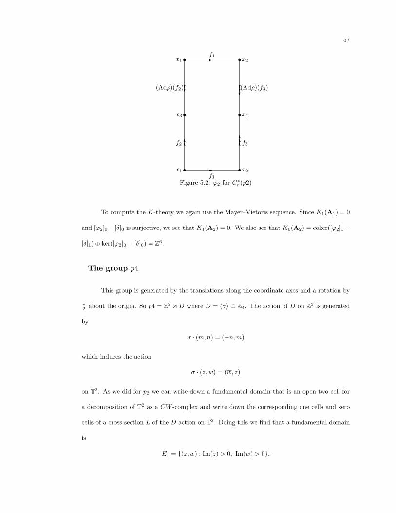
57
f1
f1
f2 f3
(Adρ)(f2) (Adρ)(f3)
•x1 •x2
•x3
•x1 •x2
•x4
-
-
66
666
??
???
Figure 5.2: ϕ2 for C∗r (p2)
To compute the K-theory we again use the Mayer–Vietoris sequence. Since K1(A1) = 0
and [ϕ2]0− [δ]0 is surjective, we see that K1(A2) = 0. We also see that K0(A2) = coker([ϕ2]1−
[δ]1)⊕ ker([ϕ2]0 − [δ]0) = Z6.
The group p4
This group is generated by the translations along the coordinate axes and a rotation by
π2 about the origin. So p4 = Z2 oD where D = 〈σ〉 ∼= Z4. The action of D on Z2 is generated
by
σ · (m,n) = (−n,m)
which induces the action
σ · (z, w) = (w, z)
on T2. As we did for p2 we can write down a fundamental domain that is an open two cell for
a decomposition of T2 as a CW -complex and write down the corresponding one cells and zero
cells of a cross section L of the D action on T2. Doing this we find that a fundamental domain
is
E1 = (z, w) : Im(z) > 0, Im(w) > 0.

58
The one cells of a cross section are given by
e1 = (z, 1) : Im(z) > 0 and e2 = (−1, w) : Im(w) > 0.
The corresponding zero cells are then x1 = (1, 1), x2 = (−1, 1), and x3 = (−1,−1). Then the
stabilizer subgroup of x1 and x3 is all of D and the stabilizer subgroup of x2 is 〈σ2〉. Thus we
let A0 = C4⊕M2(C)2⊕C4, where all are viewed as appropriate subalgebras of M4(C). Since e1
and e2 have trivial stabilizer subgroups, we let F1 = M4(C)2. Then A1 = I1F1
⊕F2
1A0 where
the connecting morphism is given by
ϕ1(x1,x2,x3) = ((x1,x2), (x2,x3)).
The Mayer–Vietoris sequence for A1 is
K1(A1) 0 0.......................................................................................................................................... ............[g2, g1]1
................................................................................................................. ............[ϕ1]1 − [δ]1
K0(A1)Z10 ⊕ Z2Z4 ......................................................................................................................................................
[g2, g1]0.............................................................................................................................
[ϕ1]0 − [δ]0
........
........
........
........
........
........
........
........
........
........
........
........
.................
............
∂
.............................................................................................................................
∂
Then [ϕ1]0 − [δ]0 is given by the matrix
1 1 1 1 0 0 0 0 0 0 −1 0
0 0 0 0 1 1 0 0 0 0 0 −1
0 0 0 0 1 1 0 0 0 0 −1 0
0 0 0 0 0 0 1 1 1 1 0 −1
.
The normal form of this matrix is given by
1 0 0 0 0 0 0 0 0 0 0 0
0 1 0 0 0 0 0 0 0 0 0 0
0 0 1 0 0 0 0 0 0 0 0 0
0 0 0 1 0 0 0 0 0 0 0 0
.
Thus we see that K0(A1) = Z8 and K1(A1) = 0.

59
Since E1 is a fundamental domain it has a trivial stabilizer subgroup, so we will let
F2 = M4(C). Then C∗r (p4) = A2 = I2F2
⊕S1F2
A1 and the connecting morphism is defined on
(f1, f2) ∈ A1 according to the following diagram:
f1
(Adρσ3)(f2)
(Adρσ)(f1) f2
•x1 •x2
•(Adρσ)(x2) •x3
-
6 66
--
Figure 5.3: ϕ2 for C∗r (p4)
From the above diagram we can see that in the Mayer–Vietoris sequence [ϕ2]1− [δ]1 = 0.
Also we know that [ϕ2]0 − [δ]0 is surjective. These facts come together to give K1(A2) = 0 and
K0(A2) = Z9.
5.3 Semidirect Products by Exactly One Reflection
The group pm
This group is generated by the translations along the coordinate axes and a reflection
across the x-axis. The action of Z2 = 〈σ〉 on Z2 is given by
σ · (m,n) = (m,−n)
which induces the action
σ · (z, w) = (z, w)
on Z2 = T2. We note at this point that the action on T2 is trivial on the first coordinate. So
we have that C∗r (pm) ∼= (C(T)⊗ C(T)) oι⊗α Z2, where the action α is the same as in example
3.1.7. Then, by Lemma 3.2.5, C∗r (pm) ∼= C(T) ⊗ C∗r (Z o Z2). Then the computation of the
K-theory reduces to that of computing the K-theory of C∗r (Z o Z2), since for any C∗-algebra

60
A we have Kn(C(T)⊗A) ∼= Kn(A)⊕Kn+1(A) (by exercise 10.1 in [29]). Then the matrix for
[ϕ1]0 − [δ]0 : Z4 ⊕ Z → Z2 is we get in the decomposition in 3.1.7 is 1 1 0 0 1
0 0 1 1 1
.
Then we see that ker [ϕ1]0 − [δ]0 = Z3∼= K0(C∗r (Z o Z2)) and K1(C∗r (Z o Z2)) = 0. So
K0(C∗r (pm)) = K1(C∗r (pm)) = Z3.
5.4 Groups Containing More Than One Reflection
Of these groups we will only work out the details for the group p4mm. p4mm is the group
generated by integer translations of the plane and the standard representation of the dihedral
group on the square [−1, 1]2. As, such it is a semidirect product Z2 oD where D = 〈σ, τ〉 ∼= D4,
where σ4 = e = τ2. Explicitly, σ is the rotation appearing in p4 and τ is the reflection appearing
in pm. The action of each element on T2 is the same as it was in p4 or pm, respectively.
Proceeding as we did for p4, a fundamental domain for the D action on T2 is given by
E1 = (z, w) : Im(z) > 0, Im(w) > 0, and Im(w) > Im(z).
The one cells are given by
e1 = (1, w) : Im(z) > 0,
e2 = (z,−1) : Im(z) > 0,
and
e3 = (z, w) : Im(z), Im(w) < 0 and z = w.
The zero cells of the decomposition are x1 = (1, 1), x2 = (−1,−1), and x3 = (1,−1). A brief
examination shows that E1 is indeed a cross section of the quotient T2 → T2/D ∼= D2.
The stabilizer subgroup of x1 and x2 is all of D4. The stabilizer subgroup of x3 is 〈τ〉.
The corresponding fixed point algebras in M8(C) are isomorphic to C2⊕C2⊕M2(C) for x1 and
x2, and M2(C)4 for x3. So we let A0 = (C2⊕C2⊕M2(C))⊕((C2⊕C2⊕M2(C))⊕(M2(C)4). The

61
one cells e1 and e3 have trivial stabilizer subgroups and e2 has 〈τ〉 as a stabilizer subgroup. Thus
we will let F1 = M8(C) ⊕ (M2(C))4 ⊕M8(C). Then A1 = I1F1
⊕F2
1A0 where the connecting
morphism is defined by ϕ1(x1,x2,x3) = ((x1,x3,x1), (x3,x2,x2)).
The Mayer–Vietoris sequence for A1 is
K1(A1) 0 0.......................................................................................................................................... ............[g2, g1]1
................................................................................................................. ............[ϕ1]1 − [δ]1
K0(A1)Z14 ⊕ Z6Z12 ......................................................................................................................................................
[g2, g1]0.............................................................................................................................
[ϕ1]0 − [δ]0
........
........
........
........
........
........
........
........
........
........
........
........
.................
............
∂
.............................................................................................................................
∂
The matrix of [ϕ1]0 − [δ]0 is
1 1 1 1 1 0 0 0 0 0 0 0 0 0 −1 0 0 0 0 0
0 0 0 0 0 1 0 0 0 0 0 0 0 0 0 −1 0 0 0 0
0 0 0 0 0 0 1 0 0 0 0 0 0 0 0 0 −1 0 0 0
0 0 0 0 0 0 0 1 0 0 0 0 0 0 0 0 0 −1 0 0
0 0 0 0 0 0 0 0 1 0 0 0 0 0 0 0 0 0 −1 0
1 1 1 1 1 0 0 0 0 0 0 0 0 0 0 0 0 0 0 −1
0 0 0 0 0 1 0 0 0 0 0 0 0 0 −1 0 0 0 0 0
0 0 0 0 0 0 1 0 0 0 0 0 0 0 0 −1 0 0 0 0
0 0 0 0 0 0 0 1 0 0 0 0 0 0 0 0 −1 0 0 0
0 0 0 0 0 0 0 0 1 0 0 0 0 0 0 0 0 −1 0 0
0 0 0 0 0 0 0 0 0 1 1 1 1 1 0 0 0 0 −1 0
0 0 0 0 0 0 0 0 0 1 1 1 1 1 0 0 0 0 0 −1
.

62
The Smith normal form of this matrix is
1 0 0 0 0 0 0 0 0 0 0 0 0 0 0 0 0 0 0 0
0 1 0 0 0 0 0 0 0 0 0 0 0 0 0 0 0 0 0 0
0 0 1 0 0 0 0 0 0 0 0 0 0 0 0 0 0 0 0 0
0 0 0 1 0 0 0 0 0 0 0 0 0 0 0 0 0 0 0 0
0 0 0 0 1 0 0 0 0 0 0 0 0 0 0 0 0 0 0 0
0 0 0 0 0 1 0 0 0 0 0 0 0 0 0 0 0 0 0 0
0 0 0 0 0 0 1 0 0 0 0 0 0 0 0 0 0 0 0 0
0 0 0 0 0 0 0 1 0 0 0 0 0 0 0 0 0 0 0 0
0 0 0 0 0 0 0 0 1 0 0 0 0 0 0 0 0 0 0 0
0 0 0 0 0 0 0 0 0 1 0 0 0 0 0 0 0 0 0 0
0 0 0 0 0 0 0 0 0 0 1 0 0 0 0 0 0 0 0 0
0 0 0 0 0 0 0 0 0 0 0 0 0 0 0 0 0 0 0 0
.
Thus we see that K1(A1) = Z and K0(A1) = Z9.
Following the pattern of p4 we let F2 = M8(C). Then C∗r (p4mm) = A2 = I2F2
⊕S1F2
A1
where the connecting morphism takes a triple (f1, f2, f3) ∈ A1 to S1F2 as in the following
diagram:
f1
f2
f3
•x1
• x2•x3
6
--
Figure 5.4: ϕ2 for C∗r (p4mm)
From the above diagram we can see that the map [ϕ2]1 − [δ]1 appearing in the Mayer–Vietoris
sequence for A2 is the identity. Since [ϕ2]0 − [δ]0 is surjective we find K0(A2) = Z9 and
K1(A2) = 0.

63
5.5 A Twisted Example
Here we will work out a decomposition and K-theory for the group pg. The group pg
acts on R2 by integer translations and the glide reflection
v 7→ v0 +Av
where v0 =
1/2
0
and A =
1 0
0 −1
. pg arises as a nonsplit extension of Z2 by Z2.
Since the corresponding crossed product is twisted we cannot apply 3.2.10 to obtain C∗r (pg)
as an NCCW -complex. We can however decompose C∗r (pg) as an NCCW -complex by using
explicit knowledge of the representation theory on the boundary of a fundamental domain for
the action of Z2 on T2 given in [35]. Obtaining NCCW decompositions for other twisted crossed
products using similar techniques seems possible; however this will have to be a topic of future
research.
First we note from [33] that C∗r (pg) ∼= F : [0, 1] × S1 → M2(C) : F (0, z), F (1, z) ∈ Rz
where Rz is the C∗-algebra consisting of matrices of the form
a zb
b a
. To decompose C∗r (pg)
we will have to realize the quotient by the ideal of functions vanishing on the ends of the cylinder
as something we recognize. Luckily this has been done for us.
Proposition 5.5.1 (Prop. 6.4.1 in [35]) There is an isomorphism from
A = F =
f1 zf2
f2 f1
∈M2(C(S1))
onto C(S1). The explicit formula for this isomorphism Φ is given by
Φ(F )(eiθ) =
f1(ei2θ)− eiθf2(ei2θ) 0 ≤ θ < π
f1(1) + f2(1) θ = π
f1(ei(2θ−2π)) + (ei(2θ−2π))12 f2(ei(2θ−2π)) π < θ ≤ 2π
Let A0 = (C2)2. Let F1 = C4 ⊕M2(C). Then let A1 be the NCCW -complex I1F1
⊕F2
1A0

64
where the connecting morphism is given by
ϕ(a, b, c, d) =
a, b, c, d,
a+b2
b−a2
b−a2
b+a2
,
b, a, d, c, c+d
2d−c2
d−c2
c+d2
.
Essentially A1 is the algebra of functions that are complex valued on two copies of S1 and
M2(C) valued on an interval, diagonal on the endpoints, arranged in such a way that we can
glue the copies of S1 to the interval by passing through each double point on the end once with
one copy of S1. This will be more clear when we write the connecting morphism for A2.
To compute the K-theory of A1 we write down the Mayer–Vietoris sequence
K1(A1) 0 0.......................................................................................................................................... ............[g2, g1]1
................................................................................................................. ............[ϕ1]1 − [δ]1
K0(A1)Z4 ⊕ Z5Z10 ......................................................................................................................................................
[g2, g1]0.............................................................................................................................
[ϕ1]0 − [δ]0
........
........
........
........
........
........
........
........
........
........
........
........
.................
............
∂
.............................................................................................................................
∂
and the matrix of [ϕ1]0 − [δ]0 is
1 0 0 0 −1 0 0 0 0
0 1 0 0 0 −1 0 0 0
0 0 1 0 0 0 −1 0 0
0 0 0 1 0 0 0 −1 0
1 1 0 0 0 0 0 0 −1
0 1 0 0 −1 0 0 0 0
1 0 0 0 0 −1 0 0 0
0 0 0 1 0 0 −1 0 0
0 0 1 0 0 0 0 −1 0
0 0 1 1 0 0 0 0 −1
.

65
The Smith normal form of this matrix is
1 0 0 0 0 0 0 0 0
0 1 0 0 0 0 0 0 0
0 0 1 0 0 0 0 0 0
0 0 0 1 0 0 0 0 0
0 0 0 0 1 0 0 0 0
0 0 0 0 0 1 0 0 0
0 0 0 0 0 0 1 0 0
0 0 0 0 0 0 0 2 0
0 0 0 0 0 0 0 0 0
0 0 0 0 0 0 0 0 0
.
So we find that K0(A1) = Z and K1(A1) = Z⊕ Z⊕ Z2.
Now let (f1, f2, f3, f4, f5) denote a generic element of A1. In order to define the connecting
morphism ϕ2 define the following two functions on S1:
g1,2(e2πit) =
f1(2t) 0 ≤ t < 1
2
f2(2t) 12 ≤ t ≤ 1
and
g3,4(e2πit) =
f3(2t) 0 ≤ t < 1
2
f4(2t) 12 ≤ t ≤ 1
Clearly every element of C(S1) will arise this way. Now let F2 = M2(C) and let A2 =
I2F2
⊕S1F2
A1, where the connecting morphism is defined by the following diagram:

66
f5
f5
Φ−1(g1,2) Φ−1(g3,4)
• •
• •
-
-
66
666
Figure 5.5: ϕ2 for C∗r (pg)
Then we have C∗r (pg) ∼= A2. By considering the definition of ϕ2 we see that in the
Mayer–Vietoris sequence for A2 we see that both [ϕ2]0 − [δ]0 and [ϕ2]1 − [δ]1 are surjective, so
K0(A2) = Z and K1(A2) = Z⊕ Z2.
5.6 The Space Group F222
In this section we will work out the K-theory for C∗r (F222), where F222 is the crystal-
lographic space group described in [2]. It is generated by the matrices
T1 =
1 0 0 0
0 1 0 1/2
0 0 1 1/2
0 0 0 1
, T2 =
1 0 0 1/2
0 1 0 0
0 0 1 1/2
0 0 0 1
, T3 =
1 0 0 1/2
0 1 0 1/2
0 0 1 0
0 0 0 1
,
U1 =
1 0 0 0
0 −1 0 0
0 0 −1 0
0 0 0 1
, U2 =
−1 0 0 0
0 1 0 0
0 0 −1 0
0 0 0 1
, U3 =
−1 0 0 0
0 −1 0 0
0 0 1 0
0 0 0 1
.
We know from [35] that C∗r (F222) is isomorphic to the crossed product C(T3) oα (Z2 × Z2),
where Z2×Z2 = 〈u1, u2〉 and the action on T3 is given by u1 ·(z, w, v) = (z, zv, zw), u2 ·(z, w, v) =
(wv,w, zw), and u1u2 · (z, w, v) = (wv, zv, v). Following the computations in both [35] and [2]
we know that C∗r (F222) is isomorphic to the following subalgebra of C(T ) ⊗M4(C), where T

67
denotes a solid tetrahedron. Let T 1 denote the one-skeleton of T . Label the vertices of T 1 by
x1, x2, x3, and x4. Label the edges of T 1 by E1, E2, · · ·E6. Then C∗r (F222) is isomorphic to a
subalgebra of C(T )⊗M4(C) that takes on values in C4 over the vertices of T 1, in M2(C)2 along
the edges of T 1, and arbitrary values in M4(C) elsewhere. Let vij denote the jth component
in C4 over the vertex xi and Eij denote the jth component in C(T 1) ⊗M2(C)2 over the edge
Ei. Then from Figure 8.a in [2] we can see that an element of C∗r (F222) restricted to T 1 must
take values at the vertices in the following way:
E11(x1) =
v11 0
0 v13
, E11(x2) =
v21 0
0 v23
E12(x1) =
v12 0
0 v14
, E12(x2) =
v22 0
0 v24
E21(x1) =
v11 0
0 v12
, E21(x3) =
v31 0
0 v32
E22(x1) =
v13 0
0 v14
, E22(x3) =
v33 0
0 v34
E31(x1) =
v11 0
0 v14
, E31(x4) =
v41 0
0 v44
E32(x1) =
v12 0
0 v13
, E32(x4) =
v42 0
0 v43
E41(x3) =
v31 0
0 v34
, E41(x2) =
v21 0
0 v24
E42(x3) =
v32 0
0 v33
, E42(x2) =
v22 0
0 v23
E51(x2) =
v21 0
0 v22
, E51(x4) =
v41 0
0 v42
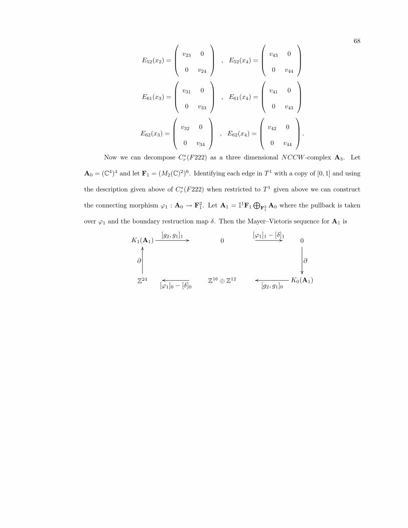
68
E52(x2) =
v23 0
0 v24
, E52(x4) =
v43 0
0 v44
E61(x3) =
v31 0
0 v33
, E61(x4) =
v41 0
0 v43
E62(x3) =
v32 0
0 v34
, E62(x4) =
v42 0
0 v44
.
Now we can decompose C∗r (F222) as a three dimensional NCCW -complex A3. Let
A0 = (C4)4 and let F1 = (M2(C)2)6. Identifying each edge in T 1 with a copy of [0, 1] and using
the description given above of C∗r (F222) when restricted to T 1 given above we can construct
the connecting morphism ϕ1 : A0 → F21. Let A1 = I1F1
⊕F2
1A0 where the pullback is taken
over ϕ1 and the boundary restruction map δ. Then the Mayer–Vietoris sequence for A1 is
K1(A1) 0 0.......................................................................................................................................... ............[g2, g1]1
................................................................................................................. ............[ϕ1]1 − [δ]1
K0(A1)Z16 ⊕ Z12Z24 ......................................................................................................................................................
[g2, g1]0.............................................................................................................................
[ϕ1]0 − [δ]0
........
........
........
........
........
........
........
........
........
........
........
........
.................
............
∂
.............................................................................................................................
∂

69
The matrix of [ϕ1]0 is
1 0 1 0 0 0 0 0 0 0 0 0 0 0 0 0 0 0 0 0 0 0 0 0 0 0 0 0
0 1 0 1 0 0 0 0 0 0 0 0 0 0 0 0 0 0 0 0 0 0 0 0 0 0 0 0
1 1 0 0 0 0 0 0 0 0 0 0 0 0 0 0 0 0 0 0 0 0 0 0 0 0 0 0
0 0 1 1 0 0 0 0 0 0 0 0 0 0 0 0 0 0 0 0 0 0 0 0 0 0 0 0
1 0 0 1 0 0 0 0 0 0 0 0 0 0 0 0 0 0 0 0 0 0 0 0 0 0 0 0
0 1 1 0 0 0 0 0 0 0 0 0 0 0 0 0 0 0 0 0 0 0 0 0 0 0 0 0
0 0 0 0 1 0 0 1 0 0 0 0 0 0 0 0 0 0 0 0 0 0 0 0 0 0 0 0
0 0 0 0 0 1 1 0 0 0 0 0 0 0 0 0 0 0 0 0 0 0 0 0 0 0 0 0
0 0 0 0 1 1 0 0 0 0 0 0 0 0 0 0 0 0 0 0 0 0 0 0 0 0 0 0
0 0 0 0 0 0 1 1 0 0 0 0 0 0 0 0 0 0 0 0 0 0 0 0 0 0 0 0
0 0 0 0 0 0 0 0 1 0 1 0 0 0 0 0 0 0 0 0 0 0 0 0 0 0 0 0
0 0 0 0 0 0 0 0 0 1 0 1 0 0 0 0 0 0 0 0 0 0 0 0 0 0 0 0
0 0 0 0 1 0 1 0 0 0 0 0 0 0 0 0 0 0 0 0 0 0 0 0 0 0 0 0
0 0 0 0 0 1 0 1 0 0 0 0 0 0 0 0 0 0 0 0 0 0 0 0 0 0 0 0
0 0 0 0 0 0 0 0 1 1 0 0 0 0 0 0 0 0 0 0 0 0 0 0 0 0 0 0
0 0 0 0 0 0 0 0 0 0 1 1 0 0 0 0 0 0 0 0 0 0 0 0 0 0 0 0
0 0 0 0 0 0 0 0 0 0 0 0 1 0 0 1 0 0 0 0 0 0 0 0 0 0 0 0
0 0 0 0 0 0 0 0 0 0 0 0 0 1 1 0 0 0 0 0 0 0 0 0 0 0 0 0
0 0 0 0 0 0 0 0 1 0 0 1 0 0 0 0 0 0 0 0 0 0 0 0 0 0 0 0
0 0 0 0 0 0 0 0 0 1 1 0 0 0 0 0 0 0 0 0 0 0 0 0 0 0 0 0
0 0 0 0 0 0 0 0 0 0 0 0 1 1 0 0 0 0 0 0 0 0 0 0 0 0 0 0
0 0 0 0 0 0 0 0 0 0 0 0 0 0 1 1 0 0 0 0 0 0 0 0 0 0 0 0
0 0 0 0 0 0 0 0 0 0 0 0 1 0 1 0 0 0 0 0 0 0 0 0 0 0 0 0
0 0 0 0 0 0 0 0 0 0 0 0 0 1 0 1 0 0 0 0 0 0 0 0 0 0 0 0
.

70
Then [ϕ1]0 − [δ]0 reduces to
1 0 0 0 0 0 0 0 0 0 0 0 0 0 0 0 0 0 0 0 0 0 0 0 0 0 0 0
0 1 0 0 0 0 0 0 0 0 0 0 0 0 0 0 0 0 0 0 0 0 0 0 0 0 0 0
0 0 1 0 0 0 0 0 0 0 0 0 0 0 0 0 0 0 0 0 0 0 0 0 0 0 0 0
0 0 0 1 0 0 0 0 0 0 0 0 0 0 0 0 0 0 0 0 0 0 0 0 0 0 0 0
0 0 0 0 1 0 0 0 0 0 0 0 0 0 0 0 0 0 0 0 0 0 0 0 0 0 0 0
0 0 0 0 0 1 0 0 0 0 0 0 0 0 0 0 0 0 0 0 0 0 0 0 0 0 0 0
0 0 0 0 0 0 1 0 0 0 0 0 0 0 0 0 0 0 0 0 0 0 0 0 0 0 0 0
0 0 0 0 0 0 0 1 0 0 0 0 0 0 0 0 0 0 0 0 0 0 0 0 0 0 0 0
0 0 0 0 0 0 0 0 1 0 0 0 0 0 0 0 0 0 0 0 0 0 0 0 0 0 0 0
0 0 0 0 0 0 0 0 0 1 0 0 0 0 0 0 0 0 0 0 0 0 0 0 0 0 0 0
0 0 0 0 0 0 0 0 0 0 1 0 0 0 0 0 0 0 0 0 0 0 0 0 0 0 0 0
0 0 0 0 0 0 0 0 0 0 0 1 0 0 0 0 0 0 0 0 0 0 0 0 0 0 0 0
0 0 0 0 0 0 0 0 0 0 0 0 1 0 0 0 0 0 0 0 0 0 0 0 0 0 0 0
0 0 0 0 0 0 0 0 0 0 0 0 0 1 0 0 0 0 0 0 0 0 0 0 0 0 0 0
0 0 0 0 0 0 0 0 0 0 0 0 0 0 1 0 0 0 0 0 0 0 0 0 0 0 0 0
0 0 0 0 0 0 0 0 0 0 0 0 0 0 0 1 0 0 0 0 0 0 0 0 0 0 0 0
0 0 0 0 0 0 0 0 0 0 0 0 0 0 0 0 1 0 0 0 0 0 0 0 0 0 0 0
0 0 0 0 0 0 0 0 0 0 0 0 0 0 0 0 0 1 0 0 0 0 0 0 0 0 0 0
0 0 0 0 0 0 0 0 0 0 0 0 0 0 0 0 0 0 1 0 0 0 0 0 0 0 0 0
0 0 0 0 0 0 0 0 0 0 0 0 0 0 0 0 0 0 0 1 0 0 0 0 0 0 0 0
0 0 0 0 0 0 0 0 0 0 0 0 0 0 0 0 0 0 0 0 2 0 0 0 0 0 0 0
0 0 0 0 0 0 0 0 0 0 0 0 0 0 0 0 0 0 0 0 0 0 0 0 0 0 0 0
0 0 0 0 0 0 0 0 0 0 0 0 0 0 0 0 0 0 0 0 0 0 0 0 0 0 0 0
0 0 0 0 0 0 0 0 0 0 0 0 0 0 0 0 0 0 0 0 0 0 0 0 0 0 0 0
.
Thus we see K0(A1) = Z7 and K1(A1) = Z3 ⊕ Z2.
To construct A2 we let F2 = M4(C)4 and define the connecting morphism ϕ2 : A1 →
S1F2 by identifying the boundary of each face of the tetrahedron with a copy of S1 in the obvious
way. Then let A2 = I2F2
⊕S1F2
A1 where the pullback is take over ϕ2 and δ. Unfortunately we
are not able to use the Mayer–Vietoris sequence to compute the K-theory of A2. This is due
to the fact that, without readily being able to identify generators of K1(A1), we are unable to
write a matrix for [ϕ2]1 − [δ]1. However we have a morphism of extensions
0 I20F2 A2 A1 0.................................................................................................... ............ ................................................................................................................. ............ .................................................................................................... ............π2 .................................................................................................... ............
0 I20F2 S2M4(C) M4(C(T 1)) 0.................................................................................................... ............ ........................................................................... ............ ...................................... ............ ............................................................... ............
.....................................................................................................
.....................................................................................................
.............................................................................................................................
.............................................................................................................................
λ

71
where the middle and right vertical maps are inclusions. Using the techniques of 3.1.2 and 4.1.1,
we see that K0(M4(C(T 1))) = Z and K1(M4(C(T 1))) = Z3. Hence we obtain the following two
six-term exact sequences for the extensions:
Z4 K0(A2) Z7.......................................................................................................................................... ............ ................................................................................................................. ............
0K1(A2)Z3 ⊕ Z2...................................................................................................................................................................................................................................................................................
........
........
........
........
........
........
........
........
........
........
........
........
.................
............
∂1
.............................................................................................................................
andZ4 K0(S2M4(C)) = Z Z.......................................................................................................................................... ............ ................................................................................................................. ............
0K1(S2M4(C)) = 0Z3 ...................................................................................................................................................................................................................................................................................
........
........
........
........
........
........
........
........
........
........
........
........
.................
............
∂′1
.............................................................................................................................
Proposition 5.6.1 K0(A2) = Z8 and K1(A2) = Z2.
Proof. By the naturality of the six-term exact sequence we have a commutative square
Z3 ⊕ Z2 Z4
Z3 Z4
.................................................................................................. ............∂1
..............................................................................................................
[λ]1
.................................................................................................. ............∂′1
..............................................................................................................
=
.
From the six term exact sequence for M4(C(T 1)) we can see that ∂′1 is injective. Then ∂1 will
be injective on Z3 if [λ]1 is injective on the torsion free part of Z3⊕Z2. Then the result follows.
To show that [λ]1 is injective first consider the injection ι : C(T ) → A1 given by
f 7→
f 0 0 0
0 0 0 0
0 0 0 0
0 0 0 0
.
From the definition of A1 we see that this maps into A1 when it is viewed as a subalgebra of
M4(C(T )). Moreover, the composition λ ι induces an isomorphism in K-theory. Hence, by
functoriality, we see that [λ]1 must be surjective. Then when we restrict [λ]1 to Z3 we see that

72
this restriction must be injective as it is a surjective map between free abelian groups of the
same rank.
Now we can proceed with the construction of A3 = C∗r (F222). Let F3 = M4(C) and
define ϕ3 : A2 → S2F3 to be the inclusion obtained be identifying the boundary of T with S2.
Then we have A3 = I3F3
⊕S2F3
A2 in the standard way. The Mayer–Vietoris sequence for the
pullback is then
K1(A3) Z2 0.......................................................................................................................................... ............[g2, g1]1
................................................................................................................. ............[ϕ3]1 − [δ]1
K0(A3)Z9Z2 ......................................................................................................................................................
[g2, g1]0.............................................................................................................................
[ϕ3]0 − [δ]0
........
........
........
........
........
........
........
........
........
........
........
........
.................
............
∂
.............................................................................................................................
∂
Then for the same reason [λ]1 was surjective in the proof of 5.6.1, we see that [ϕ3]0 − [δ]0 is
surjective. Hence K0(A3) = Z7 and K1(A3) = Z2.
Remark 5.6.2 This result differs from the result given in [35]. This is apparently because of
an error in finding the normal form of the matrix on page 105 in [35]. When we independently
used their techniques we obtained the same results as with our methods.

Bibliography
[1] W. Arveson, An Invitation to C∗-Algebras, Springer-Verlag, 1976.
[2] H. Bacry, Duals of Crystallographic Groups. Band and Quasi-Band Representations,Communications in Mathematical Physics (1993), no. 153, 359–390.
[3] B. Blackadar, K-Theory for Operator Algebras, no. 5, MSRI Publications, 1986.
[4] R. Busby and A.Smith, Representations of Twisted Group Algebras, Trans. of the AMS149 (1970), no. 2, 503–537.
[5] A. Connes, Noncommutative Geometry, Academic Press, 1994.
[6] J. Dauns and K.H. Hoffman, Representation of Rings by Sections, Memoirs of the AMS,no. 83, AMS, 1968.
[7] K. R. Davidson, C∗-Algebras by Example, Fields Institute Monographs, no. 6, AmericanMathematical Society, 1996.
[8] M.J. Dupre and R.M. Gillette, Banach Bundles, Research Notes in Mathematics, no. 92,Pitman Adv. Pub. Prog., 1983.
[9] S. Eilers, T. Loring, and G. Pedersen, Stability of Anticommutation Relations: AnApplication of Noncommutative CW Complexes, J. Reine Angew. Math. 499 (1998), 101–
143.
[10] , Morphisms of Extensions of C∗-Algebras: Pushing Forward the Busby Invariant,Advances in Mathematics 147 (1999), 74–109.
[11] G. B. Folland, A Course in Abstract Harmonic Analysis, Studies in Advanced Mathemat-ics, CRC Press, 1995.
[12] R. Fritsch and R. A. Piccinini, Cellular Structures in Topology, Cambridge Studies In Ad-vanced Mathematics, no. 19, Cambridge University Press, 1990.
[13] K. R. Goodearl, Notes on Real and Complex C∗-Algebras, Shiva Publishing Ltd., 1982.
[14] J.M. Gracia-Bondıa, J.C. Varilly, and H. Figueroa,Elements of Noncommutative Geometry, Birkhauser, 2001.
[15] P. Green, The Local Structure of Twisted Covariance Algebras, Acta Math. 140 (1978),no. 3-4, 191–250.
[16] S. Illman, Smooth Equivariant Triangulations of G-Manifolds for G a Finite Group, Math.Ann. 233 (1978), 199–220.
[17] N. Jacobson, Basic Algebra I, Freeman, 1974.

74
[18] L. C. Kinsey, Topology of Surfaces, Springer-Verlag, 1993.
[19] T. A. Loring, Lifting Solutions to Perturbing Problems in C∗ Algebras, Fields InstituteMonographs, no. 8, American Mathematical Society, 1997.
[20] W. Luck and R. Stamm, Computations of K- and L-theory for Cocompact Planar Groups,K-theory 21 (2000), no. 3, 249–292.
[21] J. R. Munkres, Topology, Prentice Hall, 2000.
[22] J. Packer and I. Raeburn, Twisted Crossed Products of C∗-algebras, Math. Proc. Camb.Phil. Soc. 106 (1989), 293–311.
[23] G. K. Pedersen, C∗-Algebras and Their Automorphism Groups, Academic Press, 1979.
[24] , Pullback and Pushout Constructions in C∗-Algebra Theory, Journal of FunctionalAnalysis 167 (1999), 243–344.
[25] I. Raeburn and D. Williams, Pull-backs of C∗-algebras and Crossed Products byCertain Diagonal Actions, Trans. Amer. Math. Soc. 287 (1985), no. 2, 755–777.
[26] I. Raeburn and D.P. Williams, Morita Equivalence and Continuous-Trace C∗-Algebras,Mathematical Surveys and Monographs, no. 60, American Mathematical Society, 1998.
[27] M. A. Rieffel, Actions of Finite Groups on C∗-Algebras, Math. Scand. (1980), no. 47, 156–176.
[28] , C∗-Algebras Associated to Irrational Rotations, Pacific Journal of Math 93(1981), no. 2, 422–423.
[29] M. Rordam, F. Larsen, and N. Lausten, An Introduction to K-theory for C∗-Algebras, Stu-dent Texts, no. 49, London Mathematical Society, 2000.
[30] C. Schochet, Topological Methods for C∗-Algebras I: Spectral Sequences, Pacific Journalof Math 96 (1981), no. 1, 193–211.
[31] , Topological Methods for C∗-Algebras III: Axiomatic Homology, Pacific Journal ofMath 114 (1984), no. 2, 399–445.
[32] R.L.E. Schwarzenberger, N-dimensional Crystallography, Research Notes in Mathematics,no. 41, Pitman Adv. Pub. Prog., 1980.
[33] K. F. Taylor, C∗-Algebras of Crystal Groups, Operator Theory: Advances and Applica-tions 41 (1989), 511–518.
[34] A. Valette, Introduction to the Baum–Connes Conjecture, Birkhauser Verlag, 2002.
[35] M. Yang, Crossed Products by Finite Groups Acting on Low Dimensional Complexesand Applications, Ph.D. thesis, Univesity of Saskatchewan, Saskatoon, 1997.

Appendix A
K-theory of Surfaces
Here we give a computation of the K-theory of any compact, connected manifold of
dimension two (which we will call a surface), using the techniques developed in this thesis.
While it is certainly plausible that these have been computed by other means, as far as we know
these results are new.
Let M be a surface. First we must realize C(M) as a two dimensional NCCW -complex.
We know, from say [18], that M arises as a certain quotient of a polygon. If M is orientable
with genus g, then the polygon is a 4g-gon, with the edges identified as follows for each copy of
T2 in the connected sum decomposition #gi=1T2.
A
AA
@@
@
e1
e−11
e2
e−12
• a
• a
• a
• a
• a
RR
U
Figure A.1: Orientable Surface Labeling Scheme
If M is nonorientable, then the identifications are made as follows for each copy of P2
appearing in the connected sum:

76
A
AA
e1
e1
• a
• a
• a
AAK
Figure A.2: Nonorientable Surface Labeling Scheme
Now we are ready to do our decompositions. First we will do the case that M is orientable
with genus g. Let A0 = C. Let F1 = C2g and A1 = I1F1
⊕F2
1A0 where the pullback is taken
over δ and ϕ1(a) = (a, a, . . . , a). Then let F2 = C and C(M) ∼= A2 = I2F2
⊕S1F2
A1. Here the
pullback is taken over the δ and ϕ2 takes (f1, f2, . . . , f2g) to the function on S1 defined by the
gluing on the edges of the 4g-gon.
In the case when M is not orientable we can make a very similar decomposition. Let m be
the number of cross-caps attached to the sphere to obtain M . Then let A0 = C and F1 = Cm.
Then A1 = I1F1
⊕F2
1A0 where the pullback is taken over δ and ϕ1(a) = (a, a, . . . , a). Then let
F2 = C and C(M) ∼= A2 = I2F2
⊕S1F2
A1. Here the pullback is taken over the δ and ϕ2 takes
(f1, f2, . . . , fm) to the function on S1 defined by the gluing on the edges of the 2m-gon. Now we
are ready to do the computations to prove the following theorem.
Theorem A.0.3 If M is an orientable surface, with genus g, then K0(C(M)) ∼= Z2 and
K1(C(M)) ∼= Z2g. If M is a nonorientable surface, obtained by attaching m cross-caps to
the sphere, then K0(C(M)) ∼= Z⊕ Z2 and K1(C(M)) ∼= Zn−1.
Proof. First suppose M is orientable and let C(M) have the aforementioned decomposition as
a two dimensional NCCW -complex. Then the Mayer–Vietoris sequence for A1 is
K1(A1) 0 0.......................................................................................................................................... ............[g2, g1]1
................................................................................................................. ............[ϕ1]− [δ]1
K0(A1)Z2g ⊕ ZZ4g ......................................................................................................................................................
[g2, g1]0.............................................................................................................................
[ϕ1]− [δ]0
........
........
........
........
........
........
........
........
........
........
........
........
.................
............
∂
.............................................................................................................................
∂

77
Then the matrix of [ϕ1]− [δ]0 is
1 −1 0 · · · 0
1 −1 0 · · · 0
1 0 −1 · · · 0
1 0 −1 · · · 0
.... . .
1 0 · · · · · · −1
1 0 · · · · · · −1
After reducing this matrix we see that K0(A1) ∼= ker([ϕ1]− [δ]0) ∼= Z
and K1(A1) ∼= Z4g/(Im([ϕ1]− [δ]0) ∼= Z2g.
The Mayer–Vietoris sequence for A2 is
K1(A2) Z2g Z.......................................................................................................................................... ............[g2, g1]1
................................................................................................................. ............[ϕ2]− [δ]1
K0(A2)Z2Z ......................................................................................................................................................
[g2, g1]0.............................................................................................................................
[ϕ2]− [δ]0
........
........
........
........
........
........
........
........
........
........
........
........
.................
............
∂
.............................................................................................................................
∂
Based on the definition of δ and ϕ2 we see that [ϕ2]− [δ]1 = 0 and that [ϕ2 − δ]0 is surjective.
So K1(A2) = K1(C(M)) ∼= Z2g and K0(C(M)) ∼= Im(∂)⊕ ker([ϕ2]− [δ]0 ∼= Z2.
If M is not orientable, with m cross-caps, then the computations are essentially the same
as the orientable case for A1. In this case we get K0(A1) = Z and K1(A1) = Zm. For A2 the
only difference from the orientable case is that [ϕ2] − [δ]1 is multiplication by 2 on one of the
generators of K1(A1) ∼= Zm, in an appropriate basis. It is still 0 on the other generators. Then
we obtain the result K1(C(M)) ∼= Zm−1 and K0(C(M)) ∼= Z⊕ Z2.
![arxiv.org · arXiv:1507.01105v3 [math-ph] 23 Jan 2017 On the Plethora of Representations Arising in Noncommutative Quantum Mechanics and An Explicit Construction of Noncommutative](https://static.fdocuments.net/doc/165x107/5e9bd85aceab874bf1154a46/arxivorg-arxiv150701105v3-math-ph-23-jan-2017-on-the-plethora-of-representations.jpg)


![S-Dualities in noncommutative and nonanticommutative field ... F-Dayi.pdf · Noncommutative space is defined by constant B : [XIL, XV] = BILv Duality can be generalized to noncommutative](https://static.fdocuments.net/doc/165x107/605cc47844073f56bf09ce8c/s-dualities-in-noncommutative-and-nonanticommutative-field-f-dayipdf-noncommutative.jpg)