Non -Uniformly Partitioned Block Convolution on …830544/FULLTEXT01.pdfcomputations of a...

Non-Uniformly Partitioned

Block Convolution on Graphics

Processing Units

Maryam Sadreddini

This thesis is presented as part of Degree of

Master of Science in Electrical Engineering

Blekinge Institute of Technology

February 2013

Blekinge Institute of Technology

School of Engineering

Department of Applied Signal Processing

Supervisors: Prof. Dr. Wlodek Kulesza

Michael Schöffler, M.Sc.

Examiner: Dr. Sven Johansson

Abstract

Real time convolution has many applications among others simulating room reverbera-

tion in audio processing. Non-uniformly partitioning filters could satisfy the both desired

features of having a low latency and less computational complexity for an efficient con-

volution. However, distributing the computation to have an uniform demand on Central

Processing Unit (CPU) is still challenging. Moreover, computational cost for very long

filters is still not acceptable. In this thesis, a new algorithm is presented by taking

advantage of the broad memory on Graphics Processing Units (GPU). Performing the

computations of a non-uniformly partitioned block convolution on GPU could solve the

problem of work load on CPU. It is shown that the computational time in this algorithm

reduces for the filters with long length.

Acknowledgements

First of all, I would like to thank my supervisor at Blekinge Institute of Technology,

Professor Dr. Wlodek Kulesza, who taught me how to be an academic researcher. His

support was always encouraging during my thesis as well as during my studies at BTH.

I would like to express my greatest gratitude to my supervisor at International Au-

dio Laboratories Erlangen (AudioLabs) in Erlangen, Germany, Michael Schoffler M.Sc.,

whom offered me this interesting topic and gave me the opportunity to do this research

under his supervision. He always guided me patiently through all the steps of this re-

search and never withheld his beneficial help. I really appreciate all the things he taught

me. I could never finish this thesis without his enlightening instructions and supports.

My special thanks goes to my husband who always stood by my side and supported me

in all the steps of this work. Last but not least, I could never thank my mother enough

for her support and encouragement during my whole life.

v

Contents

Abstract iii

Acknowledgements v

List of Figures ix

1 Introduction 1

1.1 Motivation . . . . . . . . . . . . . . . . . . . . . . . . . . . . . . . . . . . 1

1.2 Background . . . . . . . . . . . . . . . . . . . . . . . . . . . . . . . . . . . 2

1.2.1 Overlap-save method for real-time processing . . . . . . . . . . . . 4

1.3 Definitions . . . . . . . . . . . . . . . . . . . . . . . . . . . . . . . . . . . . 5

1.4 Thesis organization . . . . . . . . . . . . . . . . . . . . . . . . . . . . . . . 8

2 Survey of related works 9

2.1 Uniformly partitioning . . . . . . . . . . . . . . . . . . . . . . . . . . . . . 9

2.2 Non-uniformly partitioning . . . . . . . . . . . . . . . . . . . . . . . . . . 13

2.2.1 Efficient convolution by Gardner . . . . . . . . . . . . . . . . . . . 13

2.2.2 Multiple-FDL Convolution by Garcia . . . . . . . . . . . . . . . . . 14

2.2.3 Other Algorithms . . . . . . . . . . . . . . . . . . . . . . . . . . . . 14

3 Problem statement and main contribution 17

4 Problem solution 19

4.1 Modeling . . . . . . . . . . . . . . . . . . . . . . . . . . . . . . . . . . . . 19

4.1.1 Partitioning . . . . . . . . . . . . . . . . . . . . . . . . . . . . . . . 19

4.1.2 Scheduling . . . . . . . . . . . . . . . . . . . . . . . . . . . . . . . 21

4.1.3 Load balancing . . . . . . . . . . . . . . . . . . . . . . . . . . . . . 22

4.1.4 Multi-threading . . . . . . . . . . . . . . . . . . . . . . . . . . . . . 23

4.1.5 OpenCL framework . . . . . . . . . . . . . . . . . . . . . . . . . . 23

4.2 Implementation . . . . . . . . . . . . . . . . . . . . . . . . . . . . . . . . . 26

4.2.1 Work space . . . . . . . . . . . . . . . . . . . . . . . . . . . . . . . 26

4.2.2 Downmixing and upmixing . . . . . . . . . . . . . . . . . . . . . . 28

4.2.3 Fading . . . . . . . . . . . . . . . . . . . . . . . . . . . . . . . . . . 28

4.2.4 Architecture in CPU . . . . . . . . . . . . . . . . . . . . . . . . . . 29

4.2.5 Architecture in GPU . . . . . . . . . . . . . . . . . . . . . . . . . . 32

vii

Contents viii

5 Results 37

6 Conclusion 41

List of Figures

1.1 Filtering of data sequences . . . . . . . . . . . . . . . . . . . . . . . . . . . 3

1.2 Input signal blocks for Overlap-Save method . . . . . . . . . . . . . . . . 4

1.3 Output signal blocks for Overlap-Save method . . . . . . . . . . . . . . . 5

1.4 A Room Impulse Response with 400 milliseconds length . . . . . . . . . . 6

2.1 Long filter uniformly partitioned to four blocks and parallel structure forits convolution . . . . . . . . . . . . . . . . . . . . . . . . . . . . . . . . . 10

2.2 Steps of computing convolution by block transform . . . . . . . . . . . . . 11

2.3 Frequency-domain Delay Line (FDL) . . . . . . . . . . . . . . . . . . . . . 11

2.4 Convolution of one input channel and a BRIR filter in frequency domainusing uniform partitioning and overlap-save method . . . . . . . . . . . . 12

4.1 An example of a realizable and non-realizable partition . . . . . . . . . . . 20

4.2 An example of a realizable partition . . . . . . . . . . . . . . . . . . . . . 21

4.3 OpenCL framework . . . . . . . . . . . . . . . . . . . . . . . . . . . . . . . 24

4.4 OpenCL memory model . . . . . . . . . . . . . . . . . . . . . . . . . . . . 25

4.5 Simplified work space . . . . . . . . . . . . . . . . . . . . . . . . . . . . . 27

4.6 Linear and non-linear functions for fading . . . . . . . . . . . . . . . . . . 29

4.7 A block diagram of proposed algorithm . . . . . . . . . . . . . . . . . . . 34

5.1 Computation time for a binaural system with latency condition of 8192samples with and without cross fading . . . . . . . . . . . . . . . . . . . . 39



ix

To the love of my life, my husband, who stood by my side duringthis thesis; same as always . . .

xi

Chapter 1

Introduction

1.1 Motivation

Convolution is one of basic concepts in signal processing which has various applications.

The application which this thesis is concentrating on, is room reverberation simulation

which can be done by convolving input audio signals with Room Impulse Responses

(RIRs) which gives the impression of hearing those signals inside the target room.

A convolution could be calculated in time domain without inherent latency from direct

implementation of convolution sum. However, the computational cost of convolution for

long filters makes this computation method impractical in real time processing.

On the other hand, several methods are developed for convolving more efficiently in

frequency domain. Block transform methods based on Fast Fourier Transform (FFT)

such as overlap-save method or overlap-add method are the most common approaches.

The overlap-save method is going to be used here which collects a block of input samples

and convolves that block with a filter. The problem with this method is a large input-

output delay in case of long filters [1]. To overcome this problem, long filters can be

divided into short blocks. If the length of each block is considered equal, it is called

uniformly partitioned filter. In this way, the latency at the output decreases significantly.

However, a low latency costs computational complexity. Since the low latency is required

at the output, a hybrid model can be presented in which the impulse response of filter

has a non-uniformly partitioning ; shorter length blocks at the beginning of filter to

satisfy latency condition, and increasing block sizes at later times in the filter to reduce

computational complexity [2].

A non-uniform partitioning which has the best compromising between low computation

cost and low work load on CPU is the first objective of this thesis. We aim to show that

1

Chapter 1. Introduction 2

using the broad memory of Graphic Processing Unit (GPU) accelerates operations for

long filters.

1.2 Background

Convolution is defined as:

y(n) = x(n) ∗ h(n) =

N−1∑k=0

h(k)x(n− k) (1.1)

where x(n) is a discrete-time input signal, h(n) is an impulse response of a filter, N is the

length of h(n), and y(n) is a discrete-time output signal. The convolution summation

can easily be implemented using a direct form of Finite Impulse Response (FIR) filter.

Convolving in time domain from equation 1.1 has no inherent latency at the output.

However, by defining the computational cost of convolution as the number of multiply-

add operations per output sample, it can easily be derived that increasing the length of

filter will result in linearly increasing the computational cost. Consequently, this method

cannot be considered as a solution of performing long convolutions in real time.

There are some methods in frequency domain which are more efficient than convolution

in time domain. The Discrete Time Fourier Transform (DTFT) of a discrete sequence

converts a signal into frequency domain. The DTFT of a discrete sequence is a con-

tinuous function of frequency. In practice, the sequence x(n) is finite in duration and

the DTFT can be sampled at uniformly spaced frequencies. This sampling gives a new

transform referred to as Discrete Fourier Transform (DFT)[3].

Multiplication of the DTFTs of two signals corresponds to their linear convolution in

time domain. However, in the DFT domain, multiplication of the DFTs of two sequences

does not correspond to linear convolution but circular convolution of the two sequences,

that is,

x(n)⊗ h(n) =

N−1∑m=0

x(m)H((n−m)N )DFT⇔ X(k)H(k) (1.2)

where ⊗ denotes circular convolution, X(k) and H(k) are the N -point DFTs of x(n)

and h(n), respectively, and the notation (i)j indicates integer i modulo integer j.

Thus, the inverse DFT of X(k)H(k) cannot be used to obtain the linear convolution

of x(n) with h(n). Therefore, IDFT{X(k)H(k)} 6= x(n) ∗ h(n), where IDFT{.} in-

dicates the inverse DFT operation. However, it is possible to use DFT to compute

the linear convolution of two sequences if the two sequences are properly padded with


zeros [3]. Consider that x(n) is nonzero over the interval 0 ≤ n ≤ L − 1 and h(n)

is nonzero over the interval 0 ≤ n ≤ M − 1. If an N -point DFT is chosen such that

N ≥ M + L − 1, the circular convolution will be equivalent to linear convolution, that

is, IDFT{X(k)H(k)} = x(n) ∗h(n). The requirement that N ≥M +L− 1 comes from

the fact that the length of the output sequence resulting from linear convolution is equal

to the sum of the individual lengths of two sequences minus one.

In order to use DFT for linear convolution, let x(n) and h(n) have support as defined

in previous paragraph. Then, we can set N ≥ M + L − 1 and zero pad x(n) and h(n)

to have support n = 0, 1, . . . N − 1. The following steps must be done:

1. Take N -DFT point of x(n) to give X(k), k = 0, 1, . . . , N − 1.

2. Take N -DFT point of h(n) to give H(k), k = 0, 1, . . . , N − 1.

3. Multiply: Y (k) = X(k)H(k), k = 0, 1, . . . , N − 1.

4. Take N -IDFT point of Y (k) to give y(n), n = 0, 1, . . . , N − 1.

In practice, long data sequences needed to be filtered. That is, input signal x(n) is often

very long especially in real-time signal monitoring applications. For linear filtering via

the DFT, the signal must be limited size due to memory requirements. Therefore, we

consider N -input samples at a time. If N is too large as for long data sequences, then

there is a significant delay in processing that precludes real-time processing.

Figure 1.1: Filtering of data sequences

Therefore, as the first step for filtering of long sequences, the input signal should be

segmented into fixed-size blocks prior to processing. Afterwards, we compute DFT-

based linear filtering of each block separately via the Fast Fourier Transform (FFT)

which is an efficient algorithm for calculating DFT. For FFT to be computed more

efficiently, the length of blocks should be considered as integer powers of two. By using

FFT algorithm, the order of computational complexity for larger N will be increased

logarithmically (O(logN)), which is effectively reduced compare to linearly increasing

of computational complexity in time domain. Finally, the output blocks should be fitted

together in a way that the overall output is equivalent to the linear filtering of x(n).

The main advantage of this method is that samples of the output y(n) = h(n) ∗ x(n)

will be available real-time on a block-by-block basis.


Two main approaches to real-time linear filtering of long inputs are: Overlap-Add

method and Overlap-Save method. Overlap-save method is used in this thesis since

it does not need to buffer the result of previous block, like overlap-add method [4], and

therefore, it is easier to implement.

1.2.1 Overlap-save method for real-time processing

Overlap-Save method is also called as Overlap-Discard method[4]. Consider that we

framed our input signal, x(n), into m blocks with L points and our filter, h(n) is a

M points filter. For filtering each input block with h(n), an N -DFT is needed where

N = L+M − 1. In order to deal with aliasing corruption, the support of input blocks

should change into N points. This can be seen in Figure 1.2 where for visualisation

purpose, it is considered that M < L. Each input block xm(n) for m > 1 has an overlap

in the first M − 1 points with the last M − 1 points of the previous block xm−1(n). For

m = 1, there is no previous block. Thus the first M − 1 points are zeros. That is,

x1(n) = {0, 0, . . . , 0︸︷︷︸M − 1 zeros

, x(0), x(1), . . . , x(L− 1)}

x2(n) = {x(L−M + 1), . . . , x(L− 1)︸︷︷︸last M − 1 points from x1(n)

, x(L), . . . , x(2L− 1)}

x3(n) = {x(2L−M + 1), . . . , x(2L− 1)︸︷︷︸last M − 1 points from x2(n)

, x(2L), . . . , x(3L− 1)}

...

(1.3)

Figure 1.2: Input signal blocks for Overlap-Save method [4]

The input blocks xm(n) are now of length N and they do not need any zero-padding.

Afterwards, we take N -DFT of xm(n) to give Xm(k), k = 0, 1, . . . , N − 1.

The second step is to take an N -DFT of h(n). But, a zero-padding of h(n) is required

to change its support from M points to n = 0, 1, . . . , N − 1. Since the filter is always


the same for all the input blocks, only a one-time zero-padding is sufficient. An N -DFT

of h(n) gives H(k), k = 0, 1, . . . , N − 1.

The third step is to multiplyXm(k) andH(k) to get Ym(k) = Xm(k)H(k), k = 0, 1, . . . , N−1. Finally, to obtain the filtered input in time domain, we take N -IDFT of Ym(k) to

give ym(n), n = 0, 1, . . . , N − 1. According to Figure 1.3, the first M − 1 points of each

output block must be discarded and the remaining L points of each output block are

appended to form y(n). That is,

y1(n) = { y1(0), y1(1), . . . , y1(M − 2)︸︷︷︸M − 1 points corrupted from aliasing

, y(0), . . . , y(L− 1)}

y2(n) = { y2(0), y2(1), . . . , y2(M − 2)︸︷︷︸M − 1 points corrupted from aliasing)

, y(L), . . . , y(2L− 1)}

y3(n) = { y3(0), y3(1), . . . , y3(M − 2)︸︷︷︸M − 1 points corrupted from aliasing

, y(2L), . . . , y(3L− 1)}

...

(1.4)

Figure 1.3: Output signal blocks for Overlap-Save method [4]

1.3 Definitions

In order to avoid any misunderstanding, setting some definitions could be useful.

BRIR and HRIR

A Binaural Room Impulse Response (BRIR) consists of two Room Impulse Responses

(RIRs) for a left and right ear. Each RIR is called a filter for shorter notation. A

Head Related Impulse Response (HRIR) is a filter which corresponds to a specific head

position. The coefficients of HRIRs varies for different head positions in order to convey


the characteristics of the room for any head position. An example of RIR is shown in

Figure 1.4. From the figure, it can be seen that the impulse response of filter has large

coefficients in the beginning. As the reverberation of a signal in a room is attenuated

by passing time, the coefficients are decreasing as well.

Figure 1.4: A Room Impulse Response with 400 milliseconds length

Block

Dividing filters into shorter blocks is necessary for efficient convolution. The smallest

division of filter on which block transform is operating, is called a Block.

Partition

Filters could be divided into shorter blocks in two different main ways: uniformly, that

is when all the blocks have the same length, and non-uniformly when the size of blocks

varies. No matter how it is divided, the combination of all blocks of a filter is called a

Partition.

Segment

All blocks which have the same length create a Segment. It is clear that in uniformly

partitioning, there is only one segment in a filter’s partition. The length of blocks within

a segment is called Blocklength, and the number of existed blocks in one segment is

called Multiplicity. If the blocklength considered to be longer, then the multiplicity will

be reduced. Therefore, the number of times that overlap-save method should be applied

will be decreased and its direct effect will be decreasing the computational complexity

of the convolution. Blocklength of the first segment in a partition is restricted by the

latency condition. This condition will be clarified in Chapter 3. The motivation to


use a non-uniform partition is to decrease the computational complexity. Hence, other

segments at later times should have longer blocklength. It can directly be derived that

blocklength of segments within a partition is always an increasing sequence.

Optimal Filter Partition

There are several possible non-uniform partitioning for a filter. In order to choose

the best one, a cost analysis is needed to measure the computational costs for the

non-uniformly partition convolution. The cost function used in this thesis is the one

introduced in [5] in which the costs are assessed by the amount of computation per

output sample. This will be explained in more details in section 4.2.1.

Schedule

All blocks of a partition should be convolved with input samples. The time for convolving

each block should be chosen appropriately in a way that convolution by a block transform

starts when enough input samples are accumulated. This time will be referred to as a

starting time slot for each block. There could be latency in the result of convolving with

first block. But since the first output is generated, results should always be ready to be

heard at the output. This constraint defines a deadline for computation of each block

so that the computation must be finished before the deadline. A schedule which defines

starting time slots and deadlines for all blocks of a partition is called an acceptable

schedule.

Load Balancing

It is very important for the demand on a processor to be uniform as much as possible.

That is, the processor should have equal computation load over time. To meet this

goal, the cost function might be use again. Using different schedules, the cost function

could estimate the cost in each processing step. The schedule which results with the

lowest Mean Absolute Deviation (MAD) from the mean of cost will be chosen. Using

multi-threading on CPU could also result in better load balanced demand on CPU.


1.4 Thesis organization

The remainder of this thesis is organized as follows:

In Chapter 2, the uniformly partitioning algorithm is explained and the advantages and

disadvantages of using it is investigated. Moreover, an overview of the related works

about efficient convolution is given, using both uniform and non-uniform partitioning.

In Chapter 3, the problem is stated and the contribution of this thesis is clarified.

In Chapter 4, the modeling is given, the work space in which all the research has been

done is introduced, and the architecture of implementing the non-uniform algorithm on

both CPU and GPU is elaborated.

In Chapter 5, the result of executing the non-uniform algorithm on GPU is shown and

compared to CPU implementation.

Finally, in Chapter 6, the important conclusions are summarized and some ideas are

presented which might be beneficial for future work.

Chapter 2

Survey of related works

2.1 Uniformly partitioning

Room Impulse Responses could have duration of several seconds. An RIR of only two

seconds which has been sampled with frequency rate of 48000 Hz, has 96000 samples

and the overlap-save method needs to collect the same number of samples from the

input since the length of an input block and a filter used in the overlap-save method is

considered to be equal due to easier implementation. Therefore, there will be a delay

of 96000 samples in the results plus the calculation time. This is clearly a significant

delay in the output which is unacceptable. The solution to this problem is given by

exploiting the linearity characteristic of convolution: the filter can be partitioned into

shorter blocks and the result of each block could be calculated separately. The time

for convolving a small block of a filter is much less than convolving the whole filter.

Therefore, the latency will be decreased significantly [1].

The easiest partitioning is uniformly partitioning in which all the blocks have the same

length as equal as the length of input block. Deciding about this length depends on the

latency condition, i.e. the maximum acceptable latency for gathering the input samples.

A common size for an input signal with frequency sampling rate of 48000 Hz is 256

samples per block. Using these settings, the latency will be 25648000 ' 5.3 ms which is

easily negligible.

The linearity of convolution requires the result of convolving each block of the filter

response with the input signal to be delayed according to the position of that block

within the filter. That is, the result of convolving a block which starts at sample p

within the filter must be delayed by p samples. Summing the delayed results of all

blocks yields the output. This procedure is shown in Figure 2.1 for a filter divided into

9

Chapter 2. Survey of related works 10

four blocks. Since the partitioning is uniform, then: d3− d2 = d2− d1 = d, where d is

equal to the latency condition 5.3 milliseconds.

Figure 2.1: Long filter uniformly partitioned to four blocks (top), Parallel structurefor its convolution (bottom)

Careful attention to this procedure shows that the first block of filter should have zero

delay in its result. Since the overlap-save method imposes a delay, we need to use a

hybrid model in which the first block h0 is always be computed using the direct form

FIR filter, while the rest of blocks are convolving using the overlap-save method [1].

Although for a typical Digital Signal Processor (DSP), block transform convolution is

more efficient than direct form filtering for samples more than or equal to 64 , this is

the accepted trade off to have zero input-output delay [2].

An equal parallel structure for the blocks which are convolved using the overlap-save

method is presented in Figure 2.2. Given the samples of an input block x(n), the

computation time for each block of the filter should not exceed 5.3 milliseconds, so that

the result of each block will be ready in time to be sent to the output. Hence, the

needed delay, d = 5.3ms, for the second block (H1) is provided by the computation

time of the overlap-save method and we do not need to apply any delay for this block.

This is the case for all the blocks. Therefore, their needed delay will be subtracted by

one d. According to the linearity of convolution, a delay block could also be inserted in

the beginning of the block diagram.

Using the fact that the same input block is needed for computing the convolution of

all the blocks, a very efficient optimization is possible in a uniform partition. That is,

FFT of the input block can be calculated only once and the delay might be applied

in frequency domain. Also, one IFFT after summing all the result would be sufficient.

This optimization is called Frequency-domain Delay Line (FDL) by Garcia[2]. Using


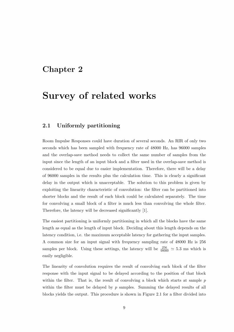
Figure 2.2: Steps of computing convolution by block transform[6]

FDL has a great effect on reducing the execution time of convolving long filters. This is

shown in Figure 2.3.

Figure 2.3: Frequency-domain Delay Line (FDL)[6]

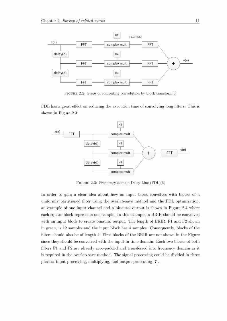
In order to gain a clear idea about how an input block convolves with blocks of a

uniformly partitioned filter using the overlap-save method and the FDL optimization,

an example of one input channel and a binaural output is shown in Figure 2.4 where

each square block represents one sample. In this example, a BRIR should be convolved

with an input block to create binaural output. The length of BRIR, F1 and F2 shown

in green, is 12 samples and the input block has 4 samples. Consequently, blocks of the

filters should also be of length 4. First blocks of the BRIR are not shown in the Figure

since they should be convolved with the input in time domain. Each two blocks of both

filters F1 and F2 are already zero-padded and transferred into frequency domain as it

is required in the overlap-save method. The signal processing could be divided in three

phases: input processing, multiplying, and output processing [7].


Figure 2.4: Convolution of one input channel and a BRIR filter in frequency domainusing uniform partitioning and overlap-save method

Input Processing

The current input block, shown in orange, should be concatenated to the previous block,

shown in dark orange, which is called recent input block. For the first time of running

when there are no recent input samples, the current block should be concatenated with

zeros of the same size. Then they should be transformed into frequency domain, shown

in blue. Afterwards, they should be inserted into the FDL’s buffer. The size of this

buffer is twice the length of all the block of the filter which should to be convolved with

the input block in the frequency domain. The reason for doubling the size is emerging

imaginary parts for each sample after taking the FFT. Before inserting the result of

FFT into the buffer, a wrapping is necessary so that the previous calculated input will

be preserved. The default values in the FDL’s buffer are all zero.

Multiplying

In this phase, the latest inserted complex values in the buffer are multiplied by the FFT

of the first block of the filter which is transformed into frequency domain. The wrapped

values of the buffer will be multiplied by the next block of the filter which corresponds

to convolving the delayed block of the input with that block. By Buffering the FDL, all

the needed convolutions are executing with only one multiplication command.


Output processing

The results of all blocks, shown in purple, should sum up and its Inverse-FFT, shown

in yellow, should be calculated. According to the overlap-save method, only the second

half of the result should be kept and the first half should be discarded. The number of

samples in the output is equal to the number of given input block as expected.

2.2 Non-uniformly partitioning

Uniformly partitioned convolution could solve the imposed problem of latency by using

the block transform. However, even after all the optimization, the computational cost is

still increasing drastically for longer filters because of increasing the number of complex

multiplication/adds. Therefore, this algorithm becomes impractical for very long room

impulse responses. In order to reduce the computational complexity, the number of

blocks should be reduced. But that is only possible if the length of each block increases

which results in an unacceptable large delay. Non-uniformly partitioning emerged to

overcome this problem.

Having low latency together with low computational complexity is only possible when

first blocks of a filter has small length and later blocks have larger length. Splitting the

filters could follow any pattern which is not uniform. Designing the best partition is the

challenge for researchers and different algorithms have been proposed. Some of these

algorithms are explained briefly in the following.

2.2.1 Efficient convolution by Gardner

Gardner was one of the very first researchers who worked on this problem. He proposed

a particular non-uniform partition in [1] in which the heading partitions have shorter

length and the length is doubled every two blocks. His goal was to achieve the result

without input-output delay. Therefore, his model is a hybrid of direct form FIR filter

for the first block and overlap-save block convolution for the rest of blocks. This idea

has been exploited in this thesis too.

Another special aspect of his model is to make the demand on the processor to become

uniform over time. He achieved this aim by setting a constraint that all the blocks of

length M , except the first one, should start at least 2M samples into the filter while

the needed time of computing output for each block should be the same amount of

waiting time for accumulating its corresponding M input samples. He also proposed a

scheduling by defining three priority levels of tasks: low priority, medium priority and


high priority. In order to have the result ready before the deadline, a high priority task

should never be interrupted. Likewise, low priority tasks should always be interrupted

before tasks with medium priority.

By this algorithm, he managed to reduce computational complexity compare to uniform

partitioning while low latency condition is not violated.

2.2.2 Multiple-FDL Convolution by Garcia

Later, Garcia presented another model in [2] called Multiple-FDL Convolution. He

correctly argued that although Gardners model was more efficient than uniformly par-

titioning, the FDL optimization used in uniformly partitioning was still a very effective

way of optimizing which could be exploited in a non-uniform partition as well. In other

words, having more multiplicities of blocks within each segment of a non-uniform parti-

tion could reduce computational complexity even more than having longer blocks with

repetition of only two times. He showed that the cost of Multiple-FDL Convolution is

more than twice as efficient as the non-uniform model given by Gardner.

This Multiple FDL model seems to be the best possible partitioning. However, deciding

about the number of segments and multiplicities is still challenging. Garcia proposed

an algorithm to find the best partition and its schedule, but only to have the lowest

computational complexity. He did not take the load of work on the processor into

account.

2.2.3 Other Algorithms

Even with the model presented by Garcia, for long filters a lot of computation is still

needed. Some studies try to reduce computational complexity such as [8]. One important

design problem in implementing the non-uniform partitioning is to obtain the correct

schedule for all blocks. However, the most challenging part is load balancing since

the computations for small blocks should be performed at every processing step, while

other blocks should wait for accumulating enough input samples. It could logically be

derived that in order to have a uniform demand on processor, the load of calculation for

longer blocks should be split within every step. It is shown in [6] that implementing a

schedule using thread synchronization always outperforms other scheduling. A thread

synchronization can be done by multi-threading in C++. It will force all the cores of

Central Processing Unit (CPU) to cooperate in computations. Also several Events will

be defined to keep track of the schedule for each block. Therefore, CPU load will be

reduced significantly. Thread synchronization will be elaborated in Chapter 4.


It is worth to mention that Non-uniformly partitioning is more competent than uniformly

partitioning only in case of having long filters. Otherwise, implementing the whole

process for non-uniformly partitioning would be more expensive than the computational

cost of the uniform partition. This is why there are still some studies on uniformly

partitioning such as [9].

Chapter 3

Problem statement and main

contribution

Although lots of efforts have been done to find an efficient non-uniformly partitioned

block convolution with an even distribution of load on the processor, it still remains as

a problem. An algorithm will be presented in this thesis for finding a partition with

minimum cost and the best scheduling to result in the best balanced load of work.

Thread synchronization plays an important role to balance the workload on CPU by

controlling the operation. However, if CPU does not have multiple cores, the thread

synchronization cannot have a strong effect. Moreover, other applications might demand

a high workload on CPU and calculating the convolution might be forced into an imposed

delay. Furthermore, calculating a convolution on multiple channel audio systems, such

as 5.1 or even 22.2 surround systems causes a very high processing load.

Using Graphic Processing Unit (GPU) as a co-processor could solve these problems.

Nowadays, many new applications are trying to take advantage of its highly parallel

structure and efficient computing capabilities for their computationally-intensive work.

Our hypothesis is that a GPU with high number of computational units could effectively

be used in vector-based operations of the convolution.

The idea of using GPU for fast convolution on uniformly partitioning was presented

in [10]. Also a comparison of highly configurable CPU and GPU convolution engine

was given in [7]. They show that in simulating a room reverberation with long filters

for multichannel systems, GPUs are necessary. However, a Non-Uniformly Partitioned

Block Convolution on GPUs was never implemented. This study is accomplished in this

thesis.

17

Chapter 4

Problem solution

4.1 Modeling

4.1.1 Partitioning

The very first designing problem for the convolution is how to split a filter into a parti-

tion. It should be noted that not all possible partitions are realizable. A block of size M

should always be placed in a partition no sooner than M samples into the filter, except

for the first block. The reason lies in two constraints. First, computation of each block

takes some time, at least one processing step, and it cannot be done instantaneously.

Second, the needed input samples for each convolving block of size M are equal to M

due to defined constraint in overlap save method. Therefore, if a block of size M placed

into a partition sooner than M samples into the filter, the result will be ready after its

deadline and nothing would be sent to the output in some steps. Clearly, this is not

desirable since it violates having no input-output delay.

Two different partitions for a filter of length 1536 are shown in Figure 4.1 which could

illustrate the difference between a realizable and non-realizable partition better. Lets

assume that an input block of 256 samples is ready and the sampling frequency is equal

to 48000 Hz. Therefore, the duration of each processing step is 5.3 milliseconds. As

mentioned in section 2.1, first blocks should always be convolved in time domain to have

zero input-output delay. Therefore, the output samples for first processing step are ready

without any delay. During listening to these results in the output, the next 256 samples of

second input block are accumulating. Meanwhile, the computation of convolving second

block of the filter with the first input block is executing. This computation should be

finished before the beginning of next processing step so that in the second processing

step, the result of second block could be heard in the output. Now, there are only 512

19

Chapter 4. Problem solution 20

samples of inputs ready and they could be convolved with third block of partition shown

in Figure 4.1(a). This computation should be finished by the end of second processing

step so that the results are ready before deadline and samples of output could be heard

during third processing step.

Figure 4.1: An example of a realizable(a) and non-realizable(b) partition

However, the third block in partition of Figure 4.1(b) requires 1024 samples of inputs to

do the calculations. Clearly, the algorithm has to wait two more processing steps until

two more input blocks are accumulated. This will cause an input-output delay since

the inputs are keeping coming while no corresponding output is generated in these two

steps. Therefore, this partition is considered as non-realizable.

An important note here is that the processor is capable of executing operations for blocks

longer than 256 samples within one processing step. It is just a matter of scheduling to

have the results ready in time. In this algorithm there is no need to the constraint given

in [1] in which computation of block size M should take time equal to the length of that

block.

Optimal partition

Once all the possible partitions are found for a filter, the optimal partition should be

chosen between them. That is, the partition for which the computational complexity

is minimum. For this purpose, a cost function is needed in order to calculate the cost

of computation for each partition. Then it is easy to select the partition which has

minimum cost. The cost function used in this thesis is the one given in [5]. They

derived this cost function based on the arithmetic complexity. The result is expressed

in floating-point operations per sample (FLOPs/sample), where FLOPs is a measure of

computer performance.

Within each partition, the cost function for each segment is defined as:

CF (b,m) = 4kFFT log2 2b+ 8m− 1 +8m− 2

b(4.1)


Where b is the blocklength of each block and m is the multiplicity of blocks within the

segment. The proportional constant kFFT depends on the efficiency of FFT which is

obtained in [5] approximately equal to 1.7. They achieved this approximation by curve

fitting for block sizes 1 ≤ N ≤ 217. Blocklengths are always considered as an integer

power of two in order to optimize the FFT calculations. The length of FFT calculated

by IPP must be a power of two. To have the overall cost of the partition, the results for

all segments should be summed up according to equation 4.2.

CF (p) :=

k∑i=1

CFi(b,m) (4.2)

Where p stands for partition and i is the number of segments. CF of different partitions

for a given filter is shown in Table 5.1.

4.1.2 Scheduling

Another important design problem is Scheduling. Even if a partition is realizable, if the

scheduler does not work properly, the same problem in Figure 4.1(b) will happen.

In order to know when a block should be calculated, a time slot should be defined

for each block to determine the processing step in which each input block should be

convolved with that block. Also, a deadline is needed to investigate that the result is

ready in time. The first block which convolves with the input in time domain does not

need a scheduler. Also the time slot for second block should always be zero so that the

calculation starts immediately. Accordingly, the deadline for second block should be

equal to 1 so that the result is ready by the end of first processing step and it could be

heard in the output during second processing step.

The example shown in Figure 4.2 could illustrate that several schedules are possible for

a partition of filter with length 4096. First block is not shown in the Figure since it does

not need a scheduler. These schedules are shown in table 4.1.

Figure 4.2: An example of a realizable partition


Table 4.1: All possible schedules for the partition given in Figure 4.2

blocks 256 256 256 512 512 1024 1024

(0,1) (0,2) (0,3) (1,4) (1,6) (3,8) (3,12)

(1,2) (1,3) (2,4) (2,6) (4,8) (4,12)

(2,3) (3,4) (3,6) (5,8) (5,12)

Possible Schedules (4,6) (6,8) (6,12)

(time slot,deadline) (5,6) (7,8) (7,12)

(8,12)

(9,12)

(10,12)

(11,12)

To sum up, each block could start its computation once enough input samples are

gathered and it must finish before the deadline. The deadline for each block is changing

non-linearly since only 256 samples will be heard in output at each processing step.

Therefore, for blocks which their prior blocklength is longer than 256, the deadline will

be increased until the step in which all previous results will be heard in the output.

The number of processing steps needed to cover all blocks of the filter can be calculated

from equation 4.3.

Numberoftimeslots = (Length of filter − length of last block)/256 + 1 (4.3)

The schedules shown in Table 4.1 are all practical without violating zero input-output

delay. But which one should be chosen in the implementation?

4.1.3 Load balancing

Clearly, an algorithm which causes a non-uniform demand on the processor is not de-

sirable. In order to avoid this situation, a load balancing is needed. Once again the

equation 4.2 will become functional. This time the cost function per cycle (processing

step) should be calculated for each schedule. By taking average of the costs between all

cycles for each schedule, Mean Absolute Deviation (MAD) could be calculated.

MAD = |average cost− cost per cycle| (4.4)


The schedule which results in lowest MAD will be chosen to gain an even distribution

of computational load.

4.1.4 Multi-threading

Every process on CPU has at least one thread. The operating system gives a small

memory to each program of the process in order to run all operations and this one

thread will keep track of them. However, in complicated programs like convolution

engine, it is not necessary for the thread to keep track of all the steps. It is possible

to define a few socket threads. Several threads could work in parallel and report their

status to these sockets. These threads are called worker threads. Whenever a new status

is reported to sockets, the main thread could intervene to manage later steps.

Multi-threading has several advantages. The most important one is that the operating

system could assign each thread to a different core of processor. If the processor has

multiple cores, this will reduce CPU load effectively. Another benefit is that the main

thread does not have to poll the socket threads constantly which would be a wasted

CPU cycle. There are two main commands at sockets sending by worker threads: signal

and wait. The main thread should go to sockets only after getting a signal command.

For convolving an input audio signal with a non-uniform partitioned filter on CPU, using

the multi-threading is crucial in order to reduce the workload.

4.1.5 OpenCL framework

OpenCL (Open Computing Language) is an open standard for general purpose paral-

lel programming on processors such as CPUs and GPUs (including both NVIDIA and

ARM) [12]. For implementing the algorithm on GPU, first we should know the charac-

teristics of this language.

As it is shown in Figure 4.3, the openCL framework consists of a context which enables

sharing memory. Different devices must be on the same context in order to be able to

compile a common code on them. In the application of this thesis, two devices are used:

Central Processing Unit (CPU) and Graphic Processing Unit (GPU). It should be noted

that a CPU or GPU with multiple cores will also be considered as one device. Therefore,

to start setting up, first the devices should be introduced to OpenCL. Then the context

should be created. For each device, at least one command queue is needed. All works

are submitted through these queues. Commands on a queue will be executed in order

unless a command is mentioned to be out of order. In that case, the run time will take


the decision that which work has priority. Other components are explained separately

in the following subsections.

Figure 4.3: OpenCL framework

Programs and Kernels

Kernels are the heart of programming which are like functions that execute on OpenCL

devices. They work based on data parallelism and task parallelism which is completely

appropriate for GPU structure with lots of computational units. A program is a col-

lection of kernels which can be considered as a dynamic library. For a program to be

executed, first it should be created by referring to the collection of kernels as the source

code. Then it should be compiled by a command of ”build” in which the devices must

be specified. If there is an error in building the program, there is a list of all possible

errors during building which makes debugging easier. Each function of the program can

be executed only when its corresponding kernel is executed.

For executing a kernel, first it should be created by giving address of the program and

name of the function corresponds to that kernel. Then the used arguments should set

and finally it should be enqueued which means that the execution command of kernel

will be sent to the command queue to wait for its turn to be executed.

It should be emphasized again that a kernel cannot be executed without building its

program first, and a program cannot be created if the source code is not a collection of

kernels. They are highly dependent to each other.


Memory objects

There are two memory resources available: Buffers and Images. For one dimensional

computations, buffers are proper. They are simple chunks of memory to which kernels

have access. A buffer can easily be created to allocate memory in a context with a

specific size and use (read or write or both). Kernels can access buffers through the

context and that is how they set their arguments and save their results. The size of

needed memory should always be given to buffers in bytes. Reading and writing in

buffers is a work which its command will also be sent to the command queue.

To have a more exact view of memory structure, memory model in OpenCL is given in

Figure 4.4. As it is shown in the Figure, transmitting data between Host(which is CPU

in this application) and the compute device (which is GPU) is only possible through

the Global or constant memory. This memory is also accessible by all work groups. In

order to accelerate the data transmission within GPU, it is better to define several work

groups. Each work group has a local memory which its size will be defined by the local

dimensions. They could also split into shorter tasks, known as work item, with specific

private memory. Only a work item has access to its private memory. Similarly, each

work group has access only to its own local memory.

Figure 4.4: OpenCL memory model


The advantage of having work groups is that synchronization becomes possible. Different

tasks could be done simultaneously within different work groups while no synchronization

is possible on global memory.

If work groups are defined, the address of local memory should also be given to the

buffer when it is creating.

Queues - Events

As it is mentioned before, each queue can execute its command in order or out of order.

For in order commands, the ordered kernel just starts executing and the run time doesn’t

necessarily wait for the result. However, if it is necessary for a code, it is possible to

lock the command queue until the results are acquired. This can be a done by a boolean

blocking option.

Events can impose an out of order command in queues. Out of order command becomes

functional when a kernel has high priority. It is possible for the run time to force that

kernel to execute at once. Events are used to control the execution between commands

and also to synchronize different queues in host and other devices. Therefore, they are

very helpful in optimization.

4.2 Implementation

4.2.1 Work space

Virtual Studio Technology (VST) is a well-known interface for audio software. The

convolution engine used for all the tests in this research is a VST plugin which runs in

AudioMulch, a windows VST host software. This plugin is capable of having any desired

number of input and output channels. Number of filters needed in the convolution engine

will be determined by the multiplication of the number of inputs and outputs. Within

the configuration of the plugin, mappings are defined to clarify which input and filter

should be convolved together and to which output channel the result should be sent.

There is also a set of Head Related Impulse Responses (HRIRs). As mentioned in the

introduction, the objective of this convolution engine is to give the impression of hearing

those signals inside a room. As one might change his head position in the room, the

same feature is available in this convolution engine. Listener’s head position can be

tracked by a webcam and the filters corresponding to that head position will be chosen


between the set of HRIRs. HRIRs existed in this convolution engine could cover the

head rotation from −45 to 45 degree with accuracy of one degree.

Due to changing the head position of listener within a process time, fading phenomenon

will happen in the sense that the result of convolving with previous filters will be atten-

uated in the outputs while the result of current filters will be intensified. This will be

done by a cross-fader which will be explained in more details later.

The explained procedure is shown in Figure 4.5 when only one input channel and two

output channels exist (Binaural output). The cylinder shown in the left side of Figure

4.5 consists of all BRIRs from which one will be chosen by filter selection according

to the head position of listener. If the head position changes, another BRIR will be

selected. Input M will be convolved with both recent and current BRIR. The results of

the left RIRs will fade by left cross-fader, and the results of the right RIRs will fade by

right cross-fader. Therefore, the listener could hear a faded output in both his right and

left ears.

Figure 4.5: The listener’s head position is tracked by a standard webcam to select theproper BRIR filters for real-time convolution. Both current and recent selected BRIRs

are convolved, followed by a crossfading for eliminating audible artifacts [7].

Block size of AudioMulch needs careful attention in the process since that should obey

the latency condition described in section 2.1. The default block size in AudioMulch

2.1.2 is equal to 256 samples which correspond to 5.3ms for sampling rate of 48000 Hz.


4.2.2 Downmixing and upmixing

As mentioned in previous section, a mapping existed within convolution engine. Accord-

ing to this mapping, each filter should only be convolved with the incoming samples from

the input channel to which it is mapped. Similarly, the result of computation should be

sent only to the output channel which the mapping has determined. If the number of

input channels are more than output channels, affectedly several results will be sent to

each output channel. Therefore, they should mix to produce the proper output. The

easiest way of downmixing is to multiply the summation of those results by a scaling

factor.

Depending on the configuration of convolution engine, filtering fewer number of input

channels and sending them to more number of output channels might also occur. This

will be done by upmixing.

4.2.3 Fading

If the head position of listener changes during listening to the room reverberation, a

fading feature is anticipated. To make this goal feasible, the prior result should be kept

for one processing step so that it could fade into the new result. Clearly, fading imposes

a need of more memory and more computations. However, it is necessary to eliminate

the audible artifacts.

Different functions could be used for fading. Here, one linear and one non-linear function

is implemented. In linear fading, result of recent output will be faded out according to

equation 4.5 and current result will be faded in according to equation 4.6. For non-linear

fading, a cosine function is used according to equations 4.7, 8. The summation of fade-in

and fade-out will be sent to the output. These functions are shown in Figure 4.6 for a

block length equal to 256.

Fade out = 1− recent result

blocklength(4.5)

Fade in =current result

blocklength(4.6)

Fade out = cos (90π × recent result180× blocklength

) (4.7)


Fade in = 1− cos (90π × recent result180× blocklength

) (4.8)

Figure 4.6: Linear (a) and non-linear (b) functions for fading

4.2.4 Architecture in CPU

Although implementing on CPU is not the aim of this thesis, this section is given in

order to get a good understanding of how complicated the algorithm on CPU is, and to

have a basis for a comparison with GPU implementation. Moreover, not all the steps of

the algorithm can be done on GPU since reading and writing on it is quite expensive.

Designing the optimal partition and convolution of the first block in time domain will

still be performed on CPU. Therefore, using CPU at some levels is inevitable.

The programming language used for CPU part in this thesis is C++ since it is im-

plemented on a wide variety of hardware and operating system platforms. Microsoft

Visual Studio is an Integrated Development Environment (IDE) with several built-in

languages including C++. The Dynamic Link Library (dll) is the plugin needed in

AudioMulch which will be created by visual studio. The library used for executing

Fast Fourier Transform (FFT) and other signal processing operations is Intel Integrated

Performance Primitives (Intel IPP) which is a software library with highly optimized

functions for this purpose [11].

A code written in C++ which is used to program an application, has several parts. Two

of them are important to mention. Constructor is the part which executes only once

in every time we run the application, and that is when the application is initializing.

Another part is the one which executes every time a new input is given to the application

during its run time. We call this part as process.

First step in the implementation is to find the optimal partition as described in section

4.1.1. Then, the FFT of all blocks should be computed for the chosen partition according


to the overlap-save method i.e. a block of size k must be appended by k zeros (zero-

padding). Then, an FFT of size 2k must be calculated. These calculations should be

done once in the constructor of code. Considering the work space described in 4.2.1,

that is a large amount of computation since there might be so many filters used in the

convolution engine, depending on the number of mappings. Moreover, the filters are

HRIRs which consist of 91 different sets of coefficients for each filter to cover the head

rotation from −45 to 45 degree. Having all these filters transformed into frequency

domain before the process starts, is really necessary.

However, the rest of computations need to be done during the process since they are

dependent on the input samples. These computations could also be divided in three

major steps same as uniformly partitioning: input processing, multiplying, and output

processing. But there are some substantial differences between these steps and the steps

explained in section 2.1.

Input processing

Unlike uniformly partitioning, a need of buffering input is perceptible here since the

length of input block should conform the length of convolving block, and blocklengths

are longer than 256 samples in later segments. Once the length of current input samples

is enough, they should be concatenated with recent ones. For the first time when there

are no recent inputs, the current block should be concatenated with zeros of the same

size. Then they are transformed into frequency domain. Afterwards, they should be

inserted into so called Frequency-domain Delay line’s buffer. Prior to the insertion, a

wrapping in the FDL’s buffer is required (see section 2.1).

Another important difference in non-uniform partition is that several FDLs are needed

i.e. one FDL with a size of twice each segment for all existing segments. However, not

all the FDLs are active when process is called. The wrapping and insertion in the FDL’s

buffer is done only in the steps where enough input samples are accumulated for each

FDL. For example, if an FDL corresponds to a segment with blocklength 1024, 4 blocks

of 256 input samples should be accumulated. Then, those samples are concatenated

with the recent block of the same size and their FFT is computed and inserted in their

corresponding buffer.

Multiplying

It should be noted that all blocks of each segment should be multiplied by their corre-

sponding buffers. Clearly, this step should also be executing only when the FDLs are


ready. In this work space, another important factor is to chose the correct transformed

filter according to the head position of listener.

Output processing

In this step, the results of all blocks from the complex multiplication of each FDL are

adding up together. Then an Inverse Fourier Transform is applied on the outcomes.

Afterwards, each sample of all the IFFT results will be added to their corresponding

samples. For sending the results to the proper output according to the mapping of

the convolution engine, after applying the coefficients due to the probable upmixing or

downmixing, the first 256 acquired samples will be sent directly. If fading is present,

then the current samples of results should be fade-in and the recent samples should be

fade-out. Summing the result of them will be sent to the output. But for the rest of

samples, a buffering in the output is needed. Other samples will be saved in this output

buffer and each 256 samples of them will respectively be added to the output at each

later processing step.

Multi-threading

The three steps mentioned above, will not be executed for all the FDLs at every call of

the process. The scheduling found according to section 4.1.3 which results in a balanced

distribution of computational load on CPU, will determine which FDL’s should be pro-

cesses. Keeping the track of this schedule is easier by using the thread synchronization.

Even for a uniformly partitioned block convolution, multi-threading could be useful to

reduce the computational load on CPU. To get a better understanding of how threads

work, a synchronization of tasks using multi-threading for both uniformly and uniformly

partitioning is explained briefly in the following.

For a uniformly partitioned convolution given in 2.1, the first socket thread can be placed

after the first phase of computation, input processing. If the input is multi-channel, then

the input samples coming from each channel can be processed in a different thread. When

the inputs arrive, these threads should begin working. The command from threads on

the socket is wait while they are computing. Once the FDL is ready, the command will

change to signal. This signal command is also a trigger for next group of threads to

begin. Another group of thread can compute the operations in phase two, multiplying.

These threads also have a socket thread. When one FDL is ready, the corresponding

multiplication could start and the processor does not have to wait for all the FDLs to

become ready. However, during the computation of second group of threads, no new


values should be inserted in FDLs. Otherwise, the previous calculated values will be over-

written. To solve this problem, the first socket thread will lock those memory objects

from use. The new calculated values should wait for the FDLs to become unlocked.

Signal command on the second socket thread will trigger the next step. A third group of

threads will do the output processing. If fading is required, the socket thread of output

should wait for the signal from fading thread workers too.

Clearly, for a non-uniform partition more number of threads are needed. One way for

splitting tasks between different threads in input processing is to define thread workers

according to the schedule. That is, all blocks with equal length which have the same

timeslot and same deadline could be placed in one thread. Once all the blocks of one FDL

is calculated, signal command can be sent to the first thread socket. Later socket threads

could be defined the same as uniformly partition. The only difference is that the number

of threads will be increased by the number of segments in each partition since several

FDLs are needed. As it may seem, synchronizing between large amount of threads is

complicated. Two different thread synchronizations for non-uniformly partitioning are

investigated in [6] .

4.2.5 Architecture in GPU

As mentioned in section 4.1.5, the language used for programming GPU is OpenCL

which its specification could be found in [12]. The basic idea in this algorithm is to

implement filtering by using the optimized non-uniform partition selected in 4.2.1 since

that was proved to be the best partition. Scheduling is not needed here since multi-

threading does not play any role due to task parallelism property of kernels. It means

that all the kernels will be running in parallel after execution, and no control is needed

for managing the order of operations. Another important property in GPU is that

having less buffers with longer size is more preferable since the kernels are working in

data parallel structure. It means that with only one kernel execution, the code will be

executed on all the data in that buffer simultaneously.

A block diagram of all processing steps is shown in Figure 4.7 to get a better overview.

In order to have a better understanding, only one HRIR with monaural input and output

is considered. In the first step, all the RIRs existed in convolution engine for every head

positions will be sent to a big memory buffer, called f , on GPU by a write command

(block a). Since block transform is required, these filters should be divided into blocks

according to the optimal partition and each one should be zero padded by its own

size (block b). Apple Inc developers provided an open source OpenCL FFT for FFT

implementation on OpenCL with high performance [13]. After taking FFT of all blocks,


the results will be saved in another memory buffer, called F , which is four times bigger

than f (block c). The reason is that the result of FFT will be returned interleaved i.e.

one real value and one imaginary. Clearly this needs a double size memory.

Later process should be done during the process. However, the required kernels should

already be created and all the needed memory buffers should be anticipated. In each

processing step, input samples should be sent to a memory in GPU (block d). As men-

tioned in section 4.2.4, buffering the inputs are necessary for a non-uniform partition.

Therefore, a kernel should be executed in order to buffer the input samples (block e).

Once enough input samples are accumulated in the buffer, another kernel should build

concatenated block form recent and current input samples (block f). Clearly, enough in-

put samples is relative for different segments. A loop should go through all the segments

of the partition to check the blocklength of each segment. An if condition inside the

loop should check whether enough input samples are acquired for each segment. After

taking FFT of the concatenated input blocks, the result should be saved in FDL (block

h). For the same reason as explained in input processing of CPU structure, a particular

FDL is needed. According to what explained here, it sounds rational to be able to save

all the result of accumulated input blocks of different size and if there was only one FDL,

the data would be over written. The later steps will only be executed for the FDLs in

which new values are inserted. Consequently, the computation for the segment with

shortest blocklength (256) will be done at all processing steps, but for other segments,

they could involve in filtering the input only when enough input samples are available.

Before inserting data in FDL, a kernel should wrap the previous data to implement

the delay of previous blocks of inputs (block g). Then the complex values achieved in

FDL should be multiplied by the complex valued resulted from FFT of filter (block

i). Obviously, the right Head-related filter should be chosen within the big memory F

which could be pointed out by an offset. Also, the FDL should only be multiplied by its

corresponding segment within the filter.

A kernel should be executed to sum up the results of all blocks in each FDL (block j).

Then an Inverse FFT of the result will be computed with OpenCL FFT provided in [13].

Considering the procedure in overlap-save method, only the second half of the results

will be kept (block k). The result of IFFT is also given in interleaved format. Therefore,

a kernel is needed to keep only the real values (block l). Having results of different sizes,

brings up the obligation of buffering output (block m).

If during computation, the head position of listener has changed, now is the time to

apply its effect. The result of buffering output form the recent head position should

be preserved in a separate buffer. A kernel will fade out the result from recent head

position while fading in the result of current one (block n).


Now the result is ready and the first 256 samples of buffered-output should be sent to

the output. This will be done by a read command to transfer them from GPU to the

output in CPU (block o). Rest of the values in buffered-output should be sent in later

steps. Each 256 samples of this buffer should be wrapped in order to get one step closer

to sending to the output (block p). In later steps, the next 256 samples of this buffered-

output will be summed up with new results and they will be sent to CPU together so

that all the results could be heard.

Figure 4.7: A block diagram of proposed algorithm

Generalizing this algorithm is easier now for more complicated structures. In case of

having multi-channel inputs and outputs, when more filters are involved, all the filters

should still be sent to one very big memory buffer and this part remains the same. But

buffering inputs should be done for each filter individually, since the convolution engine is

highly configurable and it is possible to have filters with different length. Obviously, the

partitioning will change when the length of filter changes. Therefore, different Buffers

and FDLs are needed. Consequently, the memory need will be increased and all the


memories needed form block e to block l will be multiplied by the number of filters.

Also, a special attention to mapping is needed in order to select that which filter should

be multiplied by input in block i. The needed buffer for the outputs will also increase to

the number of output mappings. For deciding about in which output-buffer the result

should be saved in block m, once again the mapping will become functional. If an output

is used in the mapping more than once, the results of each time will be added together.

Finally, the results will be sent form each output-buffer to its corresponding output in

CPU.

It should not be forgotten that for having zero input-output delay, it was required to

do the convolution for the first block of filters in time domain. This statement is still

valid. Since writing in GPU and reading from GPU is quite expensive, the convolution

in time domain should be computed in CPU same as before.

Chapter 5

Results

In this chapter, some tables and graphs are going to be presented to show how the

implementation works, and to investigate whether the results agree to the expectations

according to the hypothesis.

It was mentioned in section 4.2.1 that the best partition is chosen from the minimum

result of cost function given in equation 4.2 for each partition. The cost function is

measured in FLOPs. In order to show how it works, all possible partitions with their

costs are shown in table 5.1 for a filter of length 4096 samples. Latency condition is

considered 256 samples at frequency sampling rate of 48000 Hertz. The first block is

not shown in the table since it always has to be 256 samples and it should be filtered in

time domain.

The best partition for this example is uniformly partitioning which has the lowest cost.

This result was expected since the filter length is short. Non-uniformly partitioning is

more complicated and it can reduce computational complexity only in long filters.

The most important aim of this thesis was to show that non-uniform block convolution

for long filters on GPU is more efficient than other algorithms. In [7] it is shown that

implementing uniformly partitioning on GPU is more efficient than CPU for longer

filters. As a rule of thumb, GPU implementation for non-uniformly partitioning is also

faster especially since multi-threading for non-uniform implementation on CPU gets

even more complicated.

The computer system on which the tests were running on, has a CPU and GPU with

the following specification:

CPU: Intel (R) Xeon(R) [email protected] GHz

GPU: NVIDIA GeForce GTX 560 Ti, GF114 Revision A1

37

Chapter 5. Results 38

Table 5.1: All possible partitions for a filter of length 4096 with their computationalcosts

Possible partitions Cost [FLOPs/sample]

25615 180.66093

25613, 5121 239.61015

25611, 5122 231.56328

25611, 10241 230.34180

2569, 5123 223.51640

2569, 5121, 10241 289.29102

2567, 5124 215.46954

2567, 5122, 10241 281.24414

2567, 10242 206.22461

2565, 5125 207.42267

2565, 5123, 10241 273.19727

2565, 5121, 10242 265.17383

2563, 5126 199.37579

2563, 5124, 10241 265.15039

2563, 5122, 10242 257.12695

A filer of length 5.46133 seconds is considered as the starting filter length which has

262144 samples at frequency sampling of 48000 Hz. The filter length is chosen to be

a power of two in order to have more efficient computation. Since the implementation

in this thesis was first try of the kind, there are some memory limitations which force

us to increase the latency condition in order to investigate if the algorithm is working

properly. Therefore, the shortest block length is considered equal to 8192 samples in

Figure 5.1. It should be noted that this is just a limitation, not an error, and the result

is absolutely reliable for any latency condition. The computational cost is measured

in time by averaging the results from 25000 run to have a more solid outcome. The

system is considered to be binaural and the filter length is multiplied by two every

time. It can be seen that the computational effort on CPU becomes almost double by

doubling the filter length, while the computational cost on GPU is almost constant. Also,

the computational time on CPU increases even more when fading has to be calculated

additionally since the computational load is increasing. However, fading does not have

any affect on the computational cost on GPU.

The CPU load used by the test program during computation of uniformly partitioning

was almost 14% without fading and 25% with fading. But this load stays constant at

4% during computation on GPU.

The same experiment is done with latency condition of 16384 and 32768 samples. The

results are shown in Figures 5.2 and 5.3 respectively.


Figure 5.1: Computation time for a binaural system with latency condition of 8192samples without cross fading (a) and with cross fading (b)




The implementation which is chosen to be more efficient is the one with less computa-

tional time. Therefore, for filters with the lengths longer than the crossing points, GPU

implementation is more efficient. Obviously, the computational time should be shorter

than the length of filter to have zero delay.

As Figures show, the computational cost of non-uniformly partitioning convolution on

GPU almost stays constant while changing the filter length. This feature is of great

importance. Also the CPU load is reduced effectively compare to uniformly partitioning

convolution on CPU. The reason for having CPU load while the computation is done on

GPU is that choosing the best partition and convolving the first block in time domain

is still performed on CPU.

Chapter 6

Conclusion

In this chapter, a conclusion will be derived from the obtained result given in previous

chapters. Also, some new ideas are going to be presented for a probable future work.

It was shown in this thesis that non-uniformly partitioning could reduce computational

complexity while keeping the latency condition. Moreover, a hybrid model of convolving

in time and frequency domain was implemented to result in no input-output delay.

Furthermore, a method for choosing the best partitioning was explained. Also, the

structure of implementation on CPU was elaborated and using multi-threading was

clarified to attain a load balanced demand on CPU.

Later, it was argued that even after all the considerations, the computational complexity

for very long filters could still be problematic. Therefore, GPU was presented as a co-

processor, and the framework of openCL was explained which is used for programming on

GPU. Finally, an algorithm was presented to do the convolution by using Non-uniformly

partitioned block convolution on GPU.

As confirmed by results of Chapter 5, increasing the length of filter while using GPU

has a negligible affect on the processing time. The time will stay constant also during

convolution on multiple channel audio systems and fading procedure. Therefore, the

computational time by using GPU in non-uniformly partitioning for filters long enough

will be more efficient than using CPU. This length of filter depends on the optimal

partition chosen, the number of channels in audio system, and the presence of fading.

Task parallel and data parallel structure of GPU could result in larger efficiency when

the number of computations are more. Moreover, by using GPU the working load on

CPU will be reduced significantly.

However, there are some optimization which could be done in order to make using GPU

more efficient even for the filters with shorter length. Writing to and reading from

41

Chapter 6. Conclusion 42

GPU is the most expensive command used in the algorithm which causes the algorithm

not to work properly for shorter length filters. A future work could be implementing

a hybrid model between CPU and GPU in which blocks with shorter blocklength will

be computed on CPU and blocks with longer blocklength on GPU. This optimization

should shift the crossing on Figures of Chapter 5 on a sooner time.

Another future work could be solving the memory limitation faced in this thesis. This

could be solved by an optimization on choosing the optimal partitioning and best sched-

ule. The algorithm used in this thesis was Brute Force in which all the possible states

will be calculates and the minimum one will be chosen. Obviously, when the filter length

is large and the latency condition is small, lots of possibilities will be included and the

computation for all of them needs a lot of memory. Substituting Brute Force algorithm

with Viterbi algorithm could overcome this limitation [14].

The final outlook is implementing loadbalancing on GPU. In this thesis no loadbalancing

were considered on GPU since it consists of a broad memory and a loadbalancing algo-

rithm does not have any effect except making the algorithm more complicated. However,

there are lots of new applications such as new encoders and decoders which are trying

to make use of the memory on GPU. Therefore, a loadbalancing on GPU might become

necessary in the future.

References

[1] Gardner, W. G., ”Efficient convolution without input-output delay”, J. Audio

Eng. Soc. 43 (3), 127-136, March 1995.

[2] G. Garcia, ”Optimal filter partition for efficient convolution with short input/out-

put delay,” in Audio Engineering Society, Convention Paper 5660, 2002.

[3] John G. Proakis and Dimitris G. Manolakis, Digital Signal Procesing: Priciples,

Algorithms, and Applications, 4th edition, 2007.

[4] Deepa Kunder, ”Overlap-Save and Overlap-Add for Real-time Filtering”.

[5] F. Weferes and M. Vorlander, ”Optimal Filter Partitions for Non-Uniformly Par-

titioned Convolution”, in AES 45th Intl. Conference, Helsinki, Finland, March

2012.

[6] E. Battenberg, R. Avizienis, ”Implementing Real-Time Partitioned Convolution

Algorithms on Conventional Operating Systems”,in 14th Intl. Conference on Dig-

ital Audio Effects (DaFX-11) proceedings, Paris, France, September 2011.

[7] M. Schoeffler and W. Hess, ”A Comparison of Highly Configurable CPU- and

GPU-Based Convolution Engines”, in Audio Engineering Society Convention 133,

October 2012.

[8] G. P. M. Egelmeers and P. C. W. Sommen, ”A new method for efficient convolu-

tion in frequency domain by nonuniform partitioning for adaptive filtering,” IEEE

Transactions on Signal Processing, Vol. 44, 1996.

[9] F. Wefers and M. Vorlander, ”Optimal filter partitions for real-time FIR filter-

ing using uniformly-partitioned FFT-based convolution in the frequency-domain”,

in 14th Intl. Conference on Digital Audio Effects (DaFX-11) proceedings, Paris,

France, September 2011.

[10] F. Wefers and J. Berg, ”High-Performance Real-Time FIR-Filtering Using Fast

Convolution on Graphics Hardware”, in 13th Intl. Conference on Digital Audio

Effects (DaFX-10) proceedings, Graz, Austria, September 2010.

43

Chapter 6. Conclusion 44

[11] Intel Integrated Performance Primitives for Intel Architecture, Version 7.1

[Online]. Available: http://software.intel.com/sites/products/documentation/

doclib/ipp sa/71/ipp manual/index.htm.

[12] Khronos OpenCL Working Group, The OpenCL Specification, Version 1.2, 15

November 2011 [Online]. Available: http://www.khronos.org/opencl.

[13] Apple Inc., ”Apple OpenCL FFT”, 2012 [Online]. Available: http://developer

.apple.com/library/mac/#samplecode/OpenCL FFT/Introduction/Intro.html.

[14] L. R. Rabiner, ”A Tutorial on Hidden Markov Models and Selected Applications

in Speech Recognition”, Processing of the IEEE, 77(2):257-286, February 1989.

Non -Uniformly Partitioned Block Convolution on …830544/FULLTEXT01.pdfcomputations of a...

Documents

Transcript of Non -Uniformly Partitioned Block Convolution on …830544/FULLTEXT01.pdfcomputations of a...