SYDE 770 Image Processing

Course Project

NNoonn--PPaarraammeettrriicc PPoowweerr SSppeeccttrruumm EEssttiimmaattiioonn MMeetthhooddss

SYDE 770 Image Processing Course Project

Prof E. Jernigan

Eric Hui - 97142203 erichui@alumni.uwaterloo.ca

Thursday, December 12, 2002

- - ii

Table of Contents

1 POWER SPECTRUM ESTIMATION (PSE) ......................................................................2

1.1 PERIODOGRAM................................................................................................................. 2

1.1.1 Spectral Resolution........................................................................................................... 4

1.1.2 Asymptotic Bias............................................................................................................... 4

1.1.3 Variance ........................................................................................................................ 4

1.1.4 Complexity ..................................................................................................................... 5

1.2 MODIFIED PERIODOGRAM............................................................................................... 5

1.3 BARTLETT’S METHOD ...................................................................................................... 7

1.4 WELCH’S METHOD........................................................................................................... 8

1.5 BLACKMAN-TUKEY METHOD........................................................................................... 9

2 FEATURE EXTRACTION ................................................................................................. 12

2.1 EXPERIMENT OUTLINE .................................................................................................. 12

2.2 COMPARISON OF PSE METHODS.................................................................................... 14

2.3 CANCER DETECTION ..................................................................................................... 16

3 CONCLUSIONS...................................................................................................................20

- - iii

List of Figures

Figure 1 – Triangular Window )(kw∆ and its DTFT )( ωjeW∆ ....................................................... 3

Figure 2 – Prostate Ultrasound Image ............................................................................................ 12

Figure 3 – Outlined and Identified Prostate Ultrasound Images..................................................... 12

Figure 4 – Linearization of Power Spectrum. Left: )(ˆ ωjeP . Right: )(ˆlog20 ωjeP− .................... 13

Figure 5 – Feature Image for Slope Feature.................................................................................... 13

Figure 6 – Feature Image for Y-Intercept Feature .......................................................................... 14

Figure 7 – Cancerous part identified by Dr. Fenster....................................................................... 18

Figure 8 – Feature Images. Left: slope; Right: y-intercept............................................................. 18

Figure 9 – Processed Images. Left: before thresholding; Right: after thresholding (33/255).......... 18

Figure 10 – Cancerous part identified by Dr. Fenster..................................................................... 19

Figure 11 – Feature Images. Left: slope; Right: y-intercept........................................................... 19

Figure 12 – Processed Images. Left: before thresholding; Right: after thresholding (95/255) ........ 19

- - iv

List of Tables

Table 1 – Comparison of Truncation Windows................................................................................ 6

Table 2 – Expected Feature Values ................................................................................................ 14

Table 3 – MSE for Slope Feature ................................................................................................... 15

Table 4 – MSE for Y-Intercept Feature.......................................................................................... 15

Table 5 – Interpretation of Table 3 and Table 4............................................................................. 15

Table 6 – MSE Comparisons.......................................................................................................... 16

- - 1

Abstract

There are two purposes for this paper. One purpose is to analyze several common non-parametric power spectrum estimation (PSE) methods. Another purpose is to analyze how power spectrum can be used for feature extraction to detect cancer in an ultrasound image of a prostate.

This paper first analyzes five non-parametric PSE methods. They are: Periodogram Method, Modified Periodogram Method, Bartlett’s Method, Welch’s Method, and Blackman-Tukey Method. The methods are evaluated and compared by four characteristics: spectral resolution, asymptotic bias, variance, and complexity.

The five PSE methods were implemented in Matlab and were applied to a test ultrasound image. The resulting estimated power spectrum was linearized. The slope and the y-intercept of the linearized power spectrum were used as two feature values. The mean-squared-error was calculated in order to evaluate the performance of the five methods for this feature extraction. It was found that this particular feature extraction does not depend much on the spectral resolution and the variance of the power spectrum. Consequently, the Periodogram Method, which has the lowest complexity, is best for this feature extraction.

Lastly, the texture and the overall brightness of the image are reflected on the slope and the y-intercept of the linearized power spectrum. This paper proposes a simple but effective approach which uses these two features jointly to detect the cancerous part of the prostate.

- - 2

1 Power Spectrum Estimation (PSE)

There are mainly two types of power spectrum estimation (PSE) methods: parametric and non-parametric. In contrast to parametric methods, non-parametric methods do not make any assumptions on the data-generating process or model (e.g. autoregressive model). This paper analyzes five common non-parametric PSE methods. They are: Periodogram Method, Modified Periodogram Method, Bartlett’s Method, Welch’s Method, and Blackman-Tukey Method. All these are estimation methods. The ideal power spectrum of a signal )(nx can be computed by first finding the ideal autocorrelation )(xrx :

∑−=

∞→+

+=+=

N

NnN

x nxnxN

nxnxEr )()(12

1lim)]()([)( ααα .

This is an average computed over the infinite interval ),( ∞−∞ . However, in image processing, the signal is often of finite length because the size of any image is finite. Even with a large image, in order to make the assumption of stationarity, often only a small window of the image is considered at a time. In this paper, it is assumed that the window is small enough so that the assumption of stationary holds, allowing the autocorrelation and the power spectrum to be a Fourier Transform pair.

1.1 Periodogram

A simple-minded method of estimating the autocorrelation of a signal of finite length is called the Periodogram Method. This estimation method assumes the observed signal )(nxN is a truncated version of the originally intended signal )(nx :

)()()( nwnxnx NN = , where <≤

=otherwise

NnnwN ,0

0,1)(

The autocorrelation is calculated simply by computing the average over the finite interval as follows:

∑−−

=

+=1

0

)()(1

)(ˆα

ααN

nPer nxnx

Nr .

This is mathematically equivalent to

)()(1

)()(1

)(ˆ αααα −∗=+= ∑∞

−∞=NN

nNNPer xx

Nnxnx

Nr .

Taking the Discrete Time Fourier Transform (DTFT), the power spectrum estimated using the Periodogram Method is:

2

)(1

)(ˆ ωω jN

jPer eX

NeP = ,

where )( ωjN eX is the DTFT of the observed signal )(nxN .

The expected value of the estimated autocorrelation )(ˆ αPerr is:

- - 3

)(

)(1

)]()([1

)()(1

)](ˆ[

1

0

1

0

1

0

αα

α

ααα

α

αα

x

N

nx

N

n

N

nx

rN

N

rN

nxnxEN

nxnxN

ErE

−=

=

+=

+=

∑

∑∑−−

=

−−

=

−−

=

Thus, the estimated autocorrelation )(ˆ αPerr is the product of the ideal autocorrelation )(αxr multiplied by the triangular function )(α∆w as follows:

)()()(ˆ αα xPer rwnr ∆= , where N

Nw

αα

−=∆ )( .

The power spectrum can then be estimated by taking the DTFT of the estimated autocorrelation )(ˆ αPerr as follows:

[ ] { }[ ] { }{ }

)()(21

)()(

)(ˆ[)(ˆ)(ˆ

ωω

ω

π

αα

αα

jx

j

x

PerPerj

Per

ePeW

rwDTFT

rEDTFTrDTFTEePE

∗=

=

==

∆

∆

where { } ( ) 2

)2/sin(2/sin1

)()(

== ∆∆ ω

ωαω N

NwDTFTeW j and )}({)( αω

xj

x rDTFTeP = .

Thus, the estimated power spectrum )(ˆ ωjPer eP is equivalent to the ideal power spectrum )( ωj

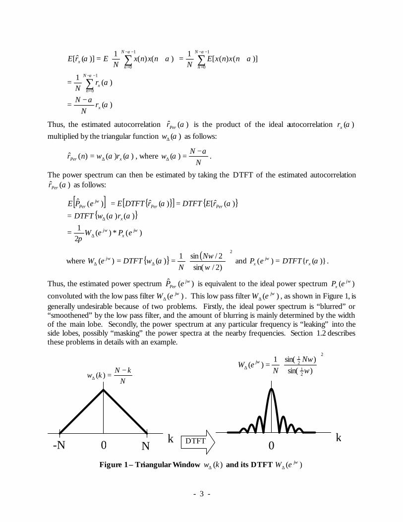
x eP convoluted with the low pass filter )( ωjeW∆ . This low pass filter )( ωjeW∆ , as shown in Figure 1, is generally undesirable because of two problems. Firstly, the ideal power spectrum is “blurred” or “smoothened” by the low pass filter, and the amount of blurring is mainly determined by the width of the main lobe. Secondly, the power spectrum at any particular frequency is “leaking” into the side lobes, possibly “masking” the power spectra at the nearby frequencies. Section 1.2 describes these problems in details with an example.

Figure 1 – Triangular Window )(kw∆ and its DTFT )( ωjeW∆

k

NkN

kw−

=∆ )(

N -N 0 0

2

21

21

)sin()sin(1

)(

=∆ ω

ωω NN

eW j

k DTFT

- - 4

In the following sections, several PSE methods, which try to improve the Periodogram Method, are described. In order to evaluate these methods, four characteristics are analyzed. They are: (1) spectral resolution, (2) asymptotic bias, (3) variance, and (4) complexity.

1.1.1 Spectral Resolution

The spectral resolution can be defined by the frequency at which the power of the low pass filter drops to half of the total power. Since 3)5.0log(20 ≈− , the spectral resolution is equivalent to the 3dB bandwidth of low pass filter. The spectral resolution measures the amount of blurring effect on the ideal power spectrum. In general, the larger the bandwidth of the main lobe, the higher spectra resolution is, and the more blurring effect the low pass filter has.

[ ] ( ) dB3)(ˆRes ωω ∆=jeP .

(Note this definition of spectral resolution might be counter-intuitive since one would normally expect the higher the spectral resolution, the sharper the spectrum would be.)

For the low pass filter )( ωjeW∆ defined above, the spectral resolution using the Periodogram Method is:

[ ]N

eP jPer

πω 289.0)(ˆRes =

Pleaser refer to [1] for derivations. For this paper, the exact derivation of this spectral resolution is not important since the spectral resolutions of all other methods are derived from this for comparison.

1.1.2 Asymptotic Bias

Another characteristic of an estimation method is asymptotic bias. One would expect that as the data length N increases, the estimated power spectrum )(ˆ ωjeP estimated should converge to the ideal power spectrum )( ωj

x eP . An estimation method is asymptotically unbiased if

[ ] )()(ˆlim ωω jx

j

NePePE =

∞→.

Using the Periodogram Method,

[ ]

∗= ∆

∞→∞→)()(

21

lim)(ˆlim ωωω

πj

xj

N

jPer

NePeWEePE

Since the low pass filter )(21 ω

πjeW∆ converges to an impulse as ∞→N , the desirable condition

[ ] )()(ˆlim ωω jjPerN

ePePE =∞→

is satisfied. Consequently, the Periodogram Method is asymptotically unbiased.

1.1.3 Variance

As the data length N increases, the variance of a desirable estimated power spectrum should vanish. Mathematically, this condition can be expressed as:

- - 5

[ ] [ ] 0)(ˆ)(ˆ)(ˆlim 21 ==∞→

ωωω jjj

NePePEePVar

Because the variance of the Periodogram Method is of fourth order, it is difficult to compute the variance for a general signal )(nx . It is shown, however, in [1] that the variance is proportional to the square of the power spectrum.

[ ] )()(ˆ 2 ωω jjPer ePePVar ≈

For example, for a Gaussian white noise process with variance 2xσ , the variance is

[ ] 0)(ˆ 4 >≈ xj

Per ePVar σω .

That is, even with a very large data length N, there are still some fluctuations or jitters in the ideally flat power spectrum.

1.1.4 Complexity

The complexity of an algorithm can be analyzed by inspecting the loop structure of the implementation. The Periodogram Method can be implemented as follows: 1) Compute the estimated autocorrelation

∑−−

=

+=1

0

)()(1

)(ˆα

ααN

nPer nxnx

Nr which is an )( 2nO operation because there are two

nested loops, one for n and one for α . 2) Take the Discrete Fourier Transform (DFT) of the estimated autocorrelation

∑−

=

−=

1

0

2

)(ˆ1

)(ˆN u

Nj

xper erN

uPα

απ

α which is an )( 2nO operation because there are two

nested loops, one for α and one for u .

Thus, the overall complexity of the Periodogram Method is )()()( 222 nOnOnO =+ .

1.2 Modified Periodogram

The Periodogram Method described above assumes that the observed signal )(nxN is a truncated version of the original intended signal )(nx , with a rectangular truncation window:

<≤

=otherwise

NnnwN ,0

0,1)( .

The Modified Periodogram generalizes the truncation window. By choosing a different truncation window, the width of the main lobe and the amplitudes of the side lobes of the low pass filtered can be varied. On one hand, the width of main lobe determines the spectral resolution. The larger the width of the main lobe, the more blurring effect the low pass filter has on the power spectrum. On the other hand, the amplitudes of the side lobes determine the spectral masking effect. The higher the amplitudes of the side lobes, the more masking effect of the power spectrum at a given frequency has on the nearby frequencies.

- - 6

Table 1 shows several common truncation windows which are defined over the finite interval 10 −≤≤ Nn .

Table 1 – Comparison of Truncation Windows

WWiinnddooww NNaammee

MMaatthhee mmaattiicc aall EExxpprreessssiioonn SSiiddee LLoobb ee LLeevveell ((ddBB))

33ddBB BBaanndd wwiiddtthh

RReeccttaa nngguull aarr WWiinnddooww

1)( =nw -13

Nπ2

89.0

TTrr iiaanngguull aarr WWiinnddooww 1

121)(

+

+−−=

N

Nnnw -27

Nπ2

28.1

HHaann nniinngg WWiinnddooww

−−=

12

cos15.0)(N

nnw

π -32

Nπ2

44.1

HHaammmmii nngg WWiinnddooww

−−=

12

cos46.054.0)(N

nnw

π -43

Nπ2

30.1

BBllaacckkmmaann WWiinnddooww

−+

−−=

14

cos8.01

2cos5.042.0)(

Nn

Nn

nwππ

-58

Nπ2

68.1

As shown from the Table 1, there is a trade-off between the width of the main lobe and the amplitudes of the side lobe. Although the Rectangular Window provides the best spectral resolution with the narrowest 3dB bandwidth for the main lobe, it also gives the worst spectral masking effect. By changing the truncation window, the spectral resolution is sacrificed for a smaller spectral masking effect.

The spectral resolution of the Modified Periodogram Method depends of the truncation window. The resolutions for the five windows are shown in Table 1. The spectral resolution is in the form:

[ ]N

eP jModified

παω 2

)(ˆRes ⋅= , where α is a window-dependent constant.

Generalizing the truncation window in the Periodogram Method,

[ ]

∗=

∞→∞→)()(

21

lim)(ˆlim ωωω

πj

xj

N

jModified

NePeWEePE .

As long as the generalized truncation window in the frequency domain )(21 ω

πjeW converges to an

impulse as ∞→N , the desirable condition

[ ] )()(ˆlim ωω jjModifiedN

ePePE =∞→

is satisfied and thus the Modified Periodogram Method is asymptotically unbiased.

The variance of the power spectrum estimated by the Modified Periodogram Method is approximately the same as that for the Periodogram Method:

[ ] )()(ˆ 2 ωω jjModified ePePVar ≈

In other words, the variance generally does not vanish even as the data length approaches infinity.

- - 7

The complexity can be analyzed by inspecting the loop structure of the implementation. The Modified Periodogram Method can be implemented as follows: 1) Compute the estimated autocorrelation

∑−−

=

++=1

0

)()()()(1

)(ˆα

αααN

nModified nxnwnxnw

Nr which is an )( 2nO operation.

2) Take the DFT of the estimated autocorrelation

∑−

=

−=

1

0

2

)(ˆ1

)(ˆN u

Nj

xModified erN

uPα

απ

α which is an )( 2nO operation.

Thus, the overall complexity of the Modified Periodogram Method is )()()( 222 nOnOnO =+ .

1.3 Bartlett’s Method

Both the Periodogram Method and Modified Periodogram Method do not give zero variances as the data length approaches infinity. One way to enforce zero variance is by averaging. The Bartlett’s Method divides the signal of length N into K segments, with each segment having length

KNL /= . The Periodogram Method is then applied to each of the K segments. The average of the resulting estimated power spectra is taken as the estimated power spectrum of the Bartlett’s Method. Mathematically, the Bartlett’s Method can be expressed as:

∑ ∑−

=

−

=

−+=1

0

isegment of mperiodogra

21

0

)(11

)(ˆK

i

L

n

jnjBartlett eiLnx

LKeP

444 3444 21

ωω

∑ ∑−

=

−

=

−+=1

0

21

0

)(1

)(ˆK

i

L

n

jnjBartlett eiLnx

NeP ωω

The spectral resolution of the estimated power spectrum )(ˆ ωjBartlett eP is determined by the

spectral resolution of each segment which is of length L . Thus, by replacing N for L in the expression in Table 1, the spectral resolution of the Bartlett’s Method is:

[ ]L

eP jBartlett

πω 289.0)(ˆRes = , but since KNL /=

[ ]N

KeP jBartlett

πω 289.0)(ˆRes ⋅= .

Each of the K segments is simply the Periodogram estimate which is asymptotically unbiased. Consequently, the estimated power spectrum )(ˆ ωj

Bartlett eP , which is the average of the Periodogram estimates of the K segments, is also asymptotically unbiased.

The variance of the estimated power spectrum )(ˆ ωjBartlett eP is:

[ ] [ ] )(1

)(ˆ1)(ˆ 2 ωωω j

xj

perj

Bartlett ePK

ePVarK

ePVari

≈= .

- - 8

Thus, as ∞→K , the variance [ ])(ˆ ωjBartlett ePVar approaches zero.

In summary, the value of K can be used to design the trade-off between spectral resolution and variance. With a larger number of segments, the variance is reduced but at the expense of spectral resolution. Conversely, with a smaller number of segments, the spectral resolution (i.e. the bandwidth of the main lobe) is reduced at expense of larger variance.

The complexity can be analyzed by inspecting the loop structure of the implementation. The Bartlett’s Method can be implemented as follows: 3) Estimate the power spectra of the K segments using the Periodogram Method. Since the

Periodogram Method is an )( 2nO operation (as described in Section 1.1.4) and is repeated K times, the complexity of this step is )()( 32 nOnOn =⋅ .

4) Compute the average of the estimates of all the segments which is an )(nO operation.

Thus, the overall complexity of the Bartlett’s Method is )()()( 33 nOnOnO =+ .

1.4 Welch’s Method

The Welch’s Method eliminates the trade off between spectral resolution and variance in the Bartlett’s Method by allowing the segments to overlap. Furthermore, the truncation window can also vary. Essentially, the Modified Periodogram Method (instead of the Periodogram Method) is applied to each of the overlapping segments. Mathematically, the estimated power spectrum

)(ˆ ωjWelch eP can be expressed as:

∑ ∑−

=

−

=

−+=1

0

21

0

)()(1

)(ˆK

i

L

n

jnjWelch eiDnxnw

KLUeP ωω , where

K is the number of segments,

L is the length of each segment,

∑−

=

=1

0

2)(

1 L

n

nwL

U ,

D is the offset between two consecutive segments; DL − is the number of overlapped points.

The spectral resolution of the estimated power spectrum )(ˆ ωjWelch eP is determined by the spectral

resolution of each segment which is of length L . It is window dependent. By replacing L for N in the expression in Table 1,

[ ]L

eP jWelch

παω 2

)(ˆRes ⋅= , but since the total data length is )1( −+= KDLN ,

[ ])1(

2)(ˆRes

−−⋅=

KDNeP j

Welchπ

αω , where α is a window-dependent constant.

- - 9

Each of the K segments is simply the Modified Periodogram estimate which is asymptotically unbiased. Consequently, the estimated power spectrum )(ˆ ωj

Welch eP , which is the average of the Periodogram estimates of the K segments, is also asymptotically unbiased.

The variance of the estimated power spectrum )(ˆ ωjWelch eP is more difficult to compute since there

is correlation between overlapping segments. However, it is shown in [1] that with 50% overlap ( LD 2

1≈ ), the variance of the estimated power spectrum )(ˆ ωjWelch eP is about:

[ ] )(169

)(ˆ 2 ωω jx

jWelch eP

NL

ePVar ≈ .

Thus, as ∞→N , the variance [ ])(ˆ ωjBartlett ePVar approaches zero.

In summary, the length of each segment, )1( −−= KDNL , can be used to improve both the spectral resolution and the variance. By allowing more overlapping (larger D ), more segments (larger K) or longer segments (larger L ) can be obtained to improve both the spectral resolution and the variance. However, overlapping introduces correlations between segments. In practice, the amount of overlapping is typically between 50% to 75% [1].

The complexity can be analyzed by inspecting the loop structure of the implementation. The Welch’s Method can be implemented as follows: 1) Estimate the power spectra of the K segments using the Modified Periodogram Method. Since

the Modified Periodogram Method is an )( 2nO operation (as described in Section 1.2) and is repeated K times, the complexity of this step is )()( 32 nOnOn =⋅ .

2) Compute the average of the estimates of all the segments which is an )(nO operation.

Thus, the overall complexity of the Welch’s Method is )()()( 33 nOnOnO =+ .

1.5 Blackman-Tukey Method

Recall that the estimated autocorrelation is:

∑−−

=

+=1

0

)()(1

)(ˆα

ααN

nx nxnx

Nr .

The estimate is worst when α is largest because the average is computed for the smallest number of terms. For example, consider the best and the worst case when 0=α and 1−= Nα ,

)1(1

)1(1

)0(1

)()(1

)0(ˆ 2221

0

−+++== ∑−

=

NxN

xN

xN

nxnxN

rN

nx K

)1()0(1

)1()(1

)1(ˆ0

0

−=−+=− ∑=

NxxN

NnxnxN

Nrn

x .

In the best case when 0=α , the autocorrelation is estimated based on the average of N terms. In the worst case when 1−= Nα , the autocorrelation is estimated based on the average of only one term. Thus, regardless how large N is, the variance of the estimated autocorrelation )(ˆ αxr , contributed mainly from the estimates where α is large (e.g. 1−≈ Nα ), still exists. The Blackman-

- - 10

Tukey Method tries to improve the estimated power spectrum by applying a window )(αBTw to )(ˆ αxr before taking the DTFT. The purpose of the window )(αBTw is to give smaller weights to

the contributions by the terms where α is large (e.g. 1−≈ Nα ).

Mathematically, the estimated power spectrum )(ˆ ωjBT eP can be expressed as:

ωω αα jkM

MkxBT

jBT erweP −

−=∑= )(ˆ)()(ˆ ,

where ],[ MM− is the support interval of the window )(αBTw with NM 21≤ . A common and

simple window would be a rectangular window, )()( αα MBT ww = , supported on interval ],[ MM− , where NM 2

1≤ . With this rectangular window )(αMw , estimates for )(ˆ αxr where M>α are ignored.

The spectral resolution of the estimated power spectrum )(ˆ ωjBT eP is window dependent. By

replacing MMM 2)( =−− for N in the expression in Table 1,

[ ]M

eP jBT 2

2)(ˆRes

παω ⋅= ,

[ ]M

eP jBT

παω 22

)(ˆRes = , where α is a window-dependent constant and NM 21≤ .

Since NM 21≤ , [ ] [ ])(ˆRes

2)(ˆRes ωω π

α jModified

jBT eP

NeP =⋅≥ , the spectral resolution is worse than

the power spectrum estimated with the Modified Periodogram Method. The higher the M value, the smaller the truncation of the estimated autocorrelation, and the better (smaller) the resolution is.

By taking the expected value and let ∞→N ,

[ ]

)()()( where,)()(21

lim

)()()(21

lim

)(ˆ)(21

lim)(ˆlim

ωωωωω

ωωω

ωωω

π

π

π

jjjBT

jx

jBTN

jx

jjBTN

jx

jBT

N

jBT

N

eWeWeWePeWE

ePeWeWE

ePeWEePE

∆∆∆∞→

∆∞→

∞→∞→

∗=

∗=

∗∗=

∗=

As long as )(21 ω

πj

BT eW ∆ converges to an impulse as ∞→N , [ ] )()(ˆlim ωω jjBTN

ePePE =∞→

,

allowing the power spectrum estimate to be asymptotically unbiased.

It is shown in [1] that the variance of the estimated power spectrum )(ˆ ωjBT eP is

[ ] ∑−=

≈M

MkBT

jx

jBT kw

NePePVar )(

1)()(ˆ 22 ωω , provided that 1>>>> MN .

Thus, the higher the M value, the larger the summation term is, giving larger variance.

- - 11

In summary, there is a trade off between spectral resolution and variance. By eliminating more components of the estimated autocorrelation (i.e. smaller M ) a smaller variance is achieved at the expensive of higher bandwidth (resolution).

The complexity can be analyzed by inspecting the loop structure of the implementation. The Blackman-Tukey Method can be implemented as follows: 1) Compute the estimated autocorrelation

∑−−

=

+=1

0

)()(1

)(ˆα

ααN

nBT nxnx

Nr which is an )( 2nO operation.

2) Multiply the estimated autocorrelation with the window )(αBTw , which is an )(nO operation. 3) Take the DFT of the estimated autocorrelation

∑−

=

−=

1

0

2

)(ˆ1

)(ˆN

n

unN

j

xBT erN

uPπ

α which is an )( 2nO operation.

Thus, the overall complexity of the Blackman-Tukey Method is )()()()( 222 nOnOnOnO =++ .

- - 12

2 Feature Extraction

A feature extraction can be thought as a mapping function that maps a region of interest (ROI) in the image space to a numerical feature value in the feature space. Inspired by [3] and [4], the linearized power spectrum of a one-dimensional scan-line of an image is used to extract two features, namely the slope and the y-intercept, as described in details below.

2.1 Experiment Outline

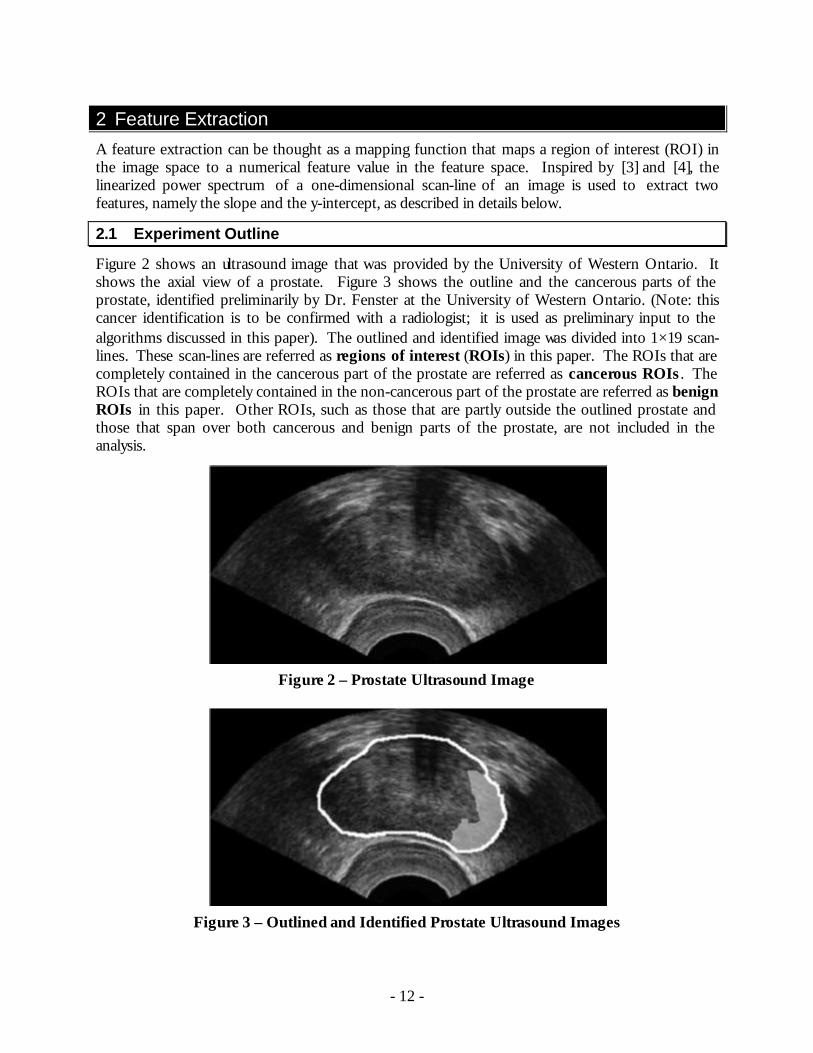
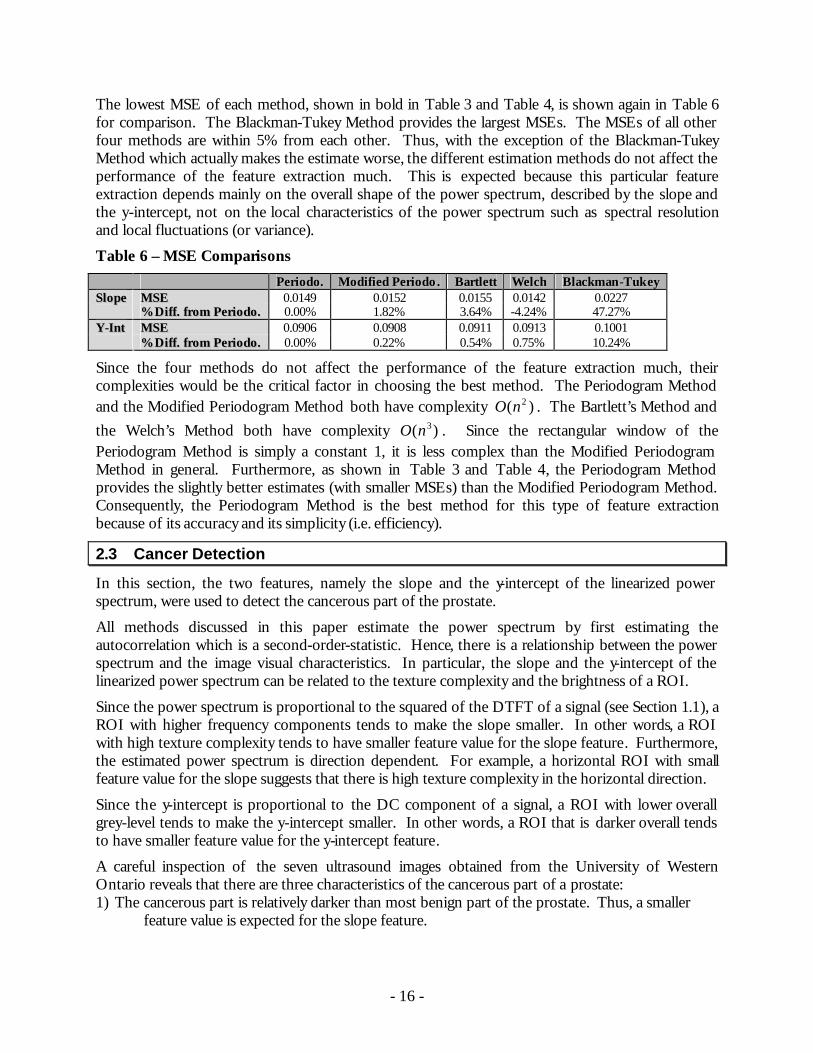
Figure 2 shows an ultrasound image that was provided by the University of Western Ontario. It shows the axial view of a prostate. Figure 3 shows the outline and the cancerous parts of the prostate, identified preliminarily by Dr. Fenster at the University of Western Ontario. (Note: this cancer identification is to be confirmed with a radiologist; it is used as preliminary input to the algorithms discussed in this paper). The outlined and identified image was divided into 1×19 scan-lines. These scan-lines are referred as regions of interest (ROIs) in this paper. The ROIs that are completely contained in the cancerous part of the prostate are referred as cancerous ROIs . The ROIs that are completely contained in the non-cancerous part of the prostate are referred as benign ROIs in this paper. Other ROIs, such as those that are partly outside the outlined prostate and those that span over both cancerous and benign parts of the prostate, are not included in the analysis.

Figure 2 – Prostate Ultrasound Image

Figure 3 – Outlined and Identified Prostate Ultrasound Images

- - 13

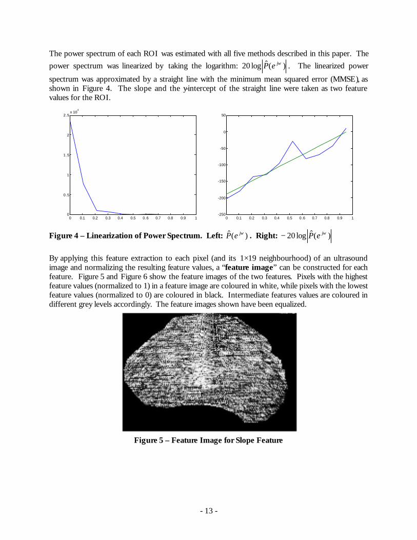
The power spectrum of each ROI was estimated with all five methods described in this paper. The power spectrum was linearized by taking the logarithm: )(ˆlog20 ωjeP . The linearized power

spectrum was approximated by a straight line with the minimum mean squared error (MMSE), as shown in Figure 4. The slope and the y-intercept of the straight line were taken as two feature values for the ROI.

Figure 4 – Linearization of Power Spectrum. Left: )(ˆ ωjeP . Right: )(ˆlog20 ωjeP−

By applying this feature extraction to each pixel (and its 1×19 neighbourhood) of an ultrasound image and normalizing the resulting feature values, a “feature image” can be constructed for each feature. Figure 5 and Figure 6 show the feature images of the two features. Pixels with the highest feature values (normalized to 1) in a feature image are coloured in white, while pixels with the lowest feature values (normalized to 0) are coloured in black. Intermediate features values are coloured in different grey levels accordingly. The feature images shown have been equalized.

Figure 5 – Feature Image for Slope Feature

0 0.1 0.2 0.3 0.4 0.5 0.6 0.7 0.8 0.9 1-250

-200

-150

-100

-50

0

50

0 0.1 0.2 0.3 0.4 0.5 0.6 0.7 0.8 0.9 10

0.5

1

1.5

2

2.5x 10

4

- - 14

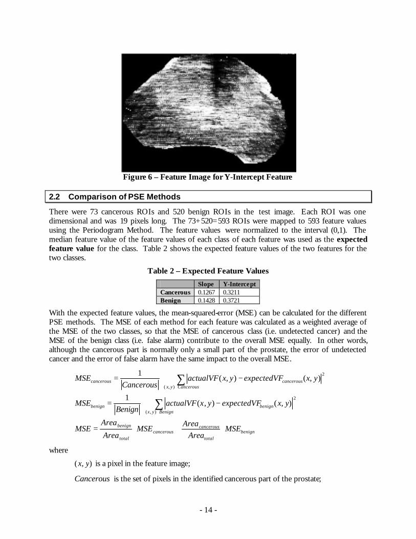
Figure 6 – Feature Image for Y-Intercept Feature

2.2 Comparison of PSE Methods

There were 73 cancerous ROIs and 520 benign ROIs in the test image. Each ROI was one dimensional and was 19 pixels long. The 73+520=593 ROIs were mapped to 593 feature values using the Periodogram Method. The feature values were normalized to the interval (0,1). The median feature value of the feature values of each class of each feature was used as the expected feature value for the class. Table 2 shows the expected feature values of the two features for the two classes.

Table 2 – Expected Feature Values

SSll ooppee YY--IInntteerrccee pptt CCaanncceerroouu ss 0.1267 0.3211 BBeenniiggnn 0.1428 0.3721

With the expected feature values, the mean-squared-error (MSE) can be calculated for the different PSE methods. The MSE of each method for each feature was calculated as a weighted average of the MSE of the two classes, so that the MSE of cancerous class (i.e. undetected cancer) and the MSE of the benign class (i.e. false alarm) contribute to the overall MSE equally. In other words, although the cancerous part is normally only a small part of the prostate, the error of undetected cancer and the error of false alarm have the same impact to the overall MSE.

benigntotal

cancerouscancerous

total

benign

Benignyxbenignbenign

Cancerousyxcancerouscancerous

MSEArea

AreaMSE

Area

AreaMSE

yxexpectedVFyxactualVFBenign

MSE

yxexpectedVFyxactualVFCancerous

MSE

⋅+⋅=

−⋅=

−⋅=

∑

∑

∈

∈

2

),(

2

),(

),(),(1

),(),(1

where

),( yx is a pixel in the feature image;

Cancerous is the set of pixels in the identified cancerous part of the prostate;

- - 15

Benign is the set of pixels in the identified benign part of the prostate;

Cancerous is the number of pixels in the set Cancerous ;

Benign is the number of pixels in the set Benign ;

),( yxactualVF is the feature value of the pixel ),( yx in the feature image;

),( yxexpectedVF is the expected feature value shown in Table 2.

The first term of the expression above represents the weighted MSE of undetected cancer. The second term represents the weighted MSE of falsely detected cancer.

Table 3 and Table 4 show the MSE for the different PSE methods of the two features. Table 5 shows the interpretation of the two tables, pointing that the Welch’s Method can be thought as a generalization of the Periodogram Method (no overlap, rectangular window), the Modified Periodogram Method (no overlap, non-rectangular window), and the Bartlett’s Method (non-zero overlap, rectangular window).

Table 3 – MSE for Slope Feature

%% OOvveerr ll aapp :: 00%% 5500%% SSeeggmmeenntt LLee nnggtt hh ((%% DD aattaa LLee nnggtt hh)) :: 110000%% 5500%% 2255%% 5500%% 2255%% WWeell cchh RReeccttaa nngguull aarr 0.0149 0.0155 0.0320 0.0142 0.0457 TTrr iiaanngguull aarr 0.0152 0.0154 0.0344 0.0305 0.0385 HHaann nniinngg 0.0281 0.0233 0.0276 0.0230 0.0251 HHaammmmii nngg 0.0265 0.0255 0.0284 0.0293 0.0324 BBll aacckkmmaann 0.0264 0.0225 0.0326 0.0225 0.0343 BBllaacckkmmaann --TTuukk eeyy 110000%% 0.0260 7755%% 0.0227 5500%% 0.0256

Table 4 – MSE for Y-Intercept Feature

%% OOvveerr ll aapp :: 00%% 5500%% SSeeggmmeenntt LLee nnggtt hh ((%% DD aattaa LLee nnggtt hh)) :: 110000%% 5500%% 2255%% 5500%% 2255%% WWeell cchh RReeccttaa nngguull aarr 0.0906 0.0911 0.1019 0.0929 0.1036 TTrr iiaanngguull aarr 0.0908 0.0913 0.1003 0.0982 0.1002 HHaann nniinngg 0.1003 0.0988 0.0969 0.0987 0.0972 HHaammmmii nngg 0.0994 0.0995 0.0991 0.0994 0.0980 BBll aacckkmmaann 0.0985 0.0959 0.1004 0.0965 0.0996 BBllaacckkmmaann --TTuukk eeyy 110000%% 0.1001 7755%% 0.1016 5500%% 0.1017

Table 5 – Interpretation of Table 3 and Table 4

%% OOvveerr ll aapp :: 00%% 5500%% SSeeggmmeenntt LLee nnggtt hh ((%% DD aattaa LLee nnggtt hh)) :: 110000%% 5500%% 2255%% 5500%% 2255%% WWeell cchh RReeccttaa nngguull aarr Periodogram Bartlett Bartlett Welch Welch TTrr iiaanngguull aarr Modified Per. Welch Welch Welch Welch HHaann nniinngg Modified Per. Welch Welch Welch Welch HHaammmmii nngg Modified Per. Welch Welch Welch Welch BBll aacckkmmaann Modified Per. Welch Welch Welch Welch BBllaacckkmmaann --TTuukk eeyy 110000%% Blackman-T. 7755%% Blackman-T. 5500%% Blackman-T.

- - 16

The lowest MSE of each method, shown in bold in Table 3 and Table 4, is shown again in Table 6 for comparison. The Blackman-Tukey Method provides the largest MSEs. The MSEs of all other four methods are within 5% from each other. Thus, with the exception of the Blackman-Tukey Method which actually makes the estimate worse, the different estimation methods do not affect the performance of the feature extraction much. This is expected because this particular feature extraction depends mainly on the overall shape of the power spectrum, described by the slope and the y-intercept, not on the local characteristics of the power spectrum such as spectral resolution and local fluctuations (or variance).

Table 6 – MSE Comparisons

PPeerr iiooddoo.. MMooddii ffiieedd PPeerr iiooddoo .. BBaarr ttll eetttt WWeell cchh BBll aacckkmmaann --TTuukk eeyy MMSSEE 0.0149 0.0152 0.0155 0.0142 0.0227 SSllooppee %% DDii ffff.. ffrroomm PPeerr iiooddoo.. 0.00% 1.82% 3.64% -4.24% 47.27% MMSSEE 0.0906 0.0908 0.0911 0.0913 0.1001 YY--IInntt %% DDii ffff.. ffrroomm PPeerr iiooddoo.. 0.00% 0.22% 0.54% 0.75% 10.24%

Since the four methods do not affect the performance of the feature extraction much, their complexities would be the critical factor in choosing the best method. The Periodogram Method and the Modified Periodogram Method both have complexity )( 2nO . The Bartlett’s Method and the Welch’s Method both have complexity )( 3nO . Since the rectangular window of the Periodogram Method is simply a constant 1, it is less complex than the Modified Periodogram Method in general. Furthermore, as shown in Table 3 and Table 4, the Periodogram Method provides the slightly better estimates (with smaller MSEs) than the Modified Periodogram Method. Consequently, the Periodogram Method is the best method for this type of feature extraction because of its accuracy and its simplicity (i.e. efficiency).

2.3 Cancer Detection

In this section, the two features, namely the slope and the y-intercept of the linearized power spectrum, were used to detect the cancerous part of the prostate.

All methods discussed in this paper estimate the power spectrum by first estimating the autocorrelation which is a second-order-statistic. Hence, there is a relationship between the power spectrum and the image visual characteristics. In particular, the slope and the y-intercept of the linearized power spectrum can be related to the texture complexity and the brightness of a ROI.

Since the power spectrum is proportional to the squared of the DTFT of a signal (see Section 1.1), a ROI with higher frequency components tends to make the slope smaller. In other words, a ROI with high texture complexity tends to have smaller feature value for the slope feature. Furthermore, the estimated power spectrum is direction dependent. For example, a horizontal ROI with small feature value for the slope suggests that there is high texture complexity in the horizontal direction.

Since the y-intercept is proportional to the DC component of a signal, a ROI with lower overall grey-level tends to make the y-intercept smaller. In other words, a ROI that is darker overall tends to have smaller feature value for the y-intercept feature.

A careful inspection of the seven ultrasound images obtained from the University of Western Ontario reveals that there are three characteristics of the cancerous part of a prostate: 1) The cancerous part is relatively darker than most benign part of the prostate. Thus, a smaller

feature value is expected for the slope feature.

- - 17

2) There are relatively more granule patterns in the cancerous part of the prostate. Thus, a smaller feature value is expected for the y-intercept feature.

3) Cancer is more likely to be found in the part of the prostate that is closer to the anus (bottom of the image). In this part of the prostate, the granule patterns look more vertical than horizontal, making the texture complexity higher in the horizontal direction than in the vertical direction. Thus, it is expected that the y-intercept feature in the horizontal direction can help detecting cancer better.

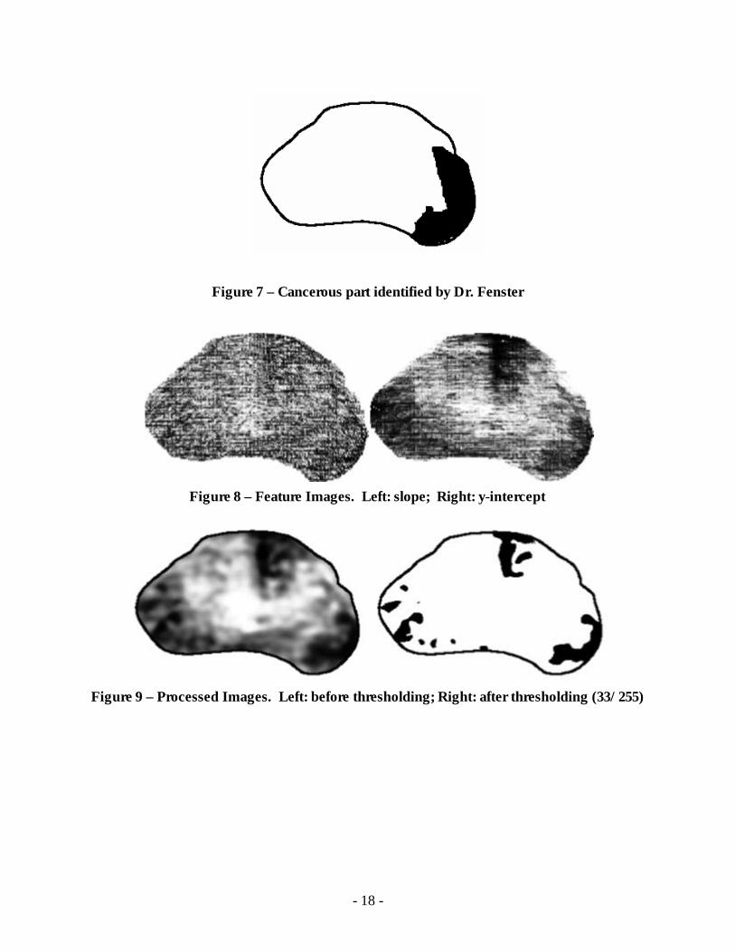
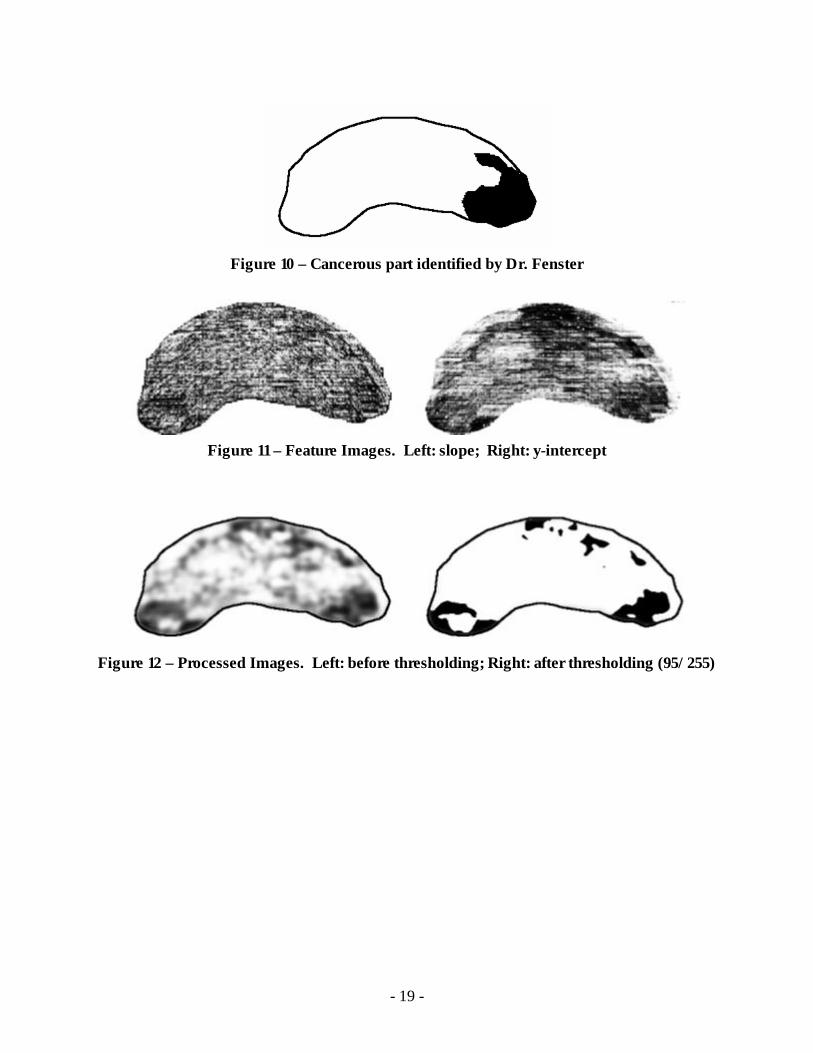
Thus, in order to detect cancer effectively, the slope feature and the y-intercept (for the horizontal direction) feature must be used jointly. This requires transforming the feature values so that the ideal cancerous feature value is logic-TRUE and the ideal benign feature value is logic-FALSE, then applying a logic-AND operator to the two features. The numerical values 1 and 0 can be used for logic-TRUE and logic-FALSE. The numerical multiplication can be used to simulate the logic-AND operator. A simple, but effective, approach was applied using Photoshop for two ultrasound images. Figure 9 and Figure 12 show the resulting images, which were processed as follows: 1) Blur the two feature images with a Gaussian blur (with variance of 4 pixels). This is justified by

the assumption that no single pixel is cancerous by itself. 2) Equalize the two blurred images so there is a high contrast. 3) Invert the two equalized images so that cancerous feature value is about 1 (as opposed to 0). 4) Multiply the two inverted images together to simulate logic-AND. 5) Equalize the resulting image so there is a high contrast. 6) Invert the image back so the cancerous part is shown as black. 7) Apply thresholding with a threshold value that is experimentally determined.

Although the results (Figure 9 and Figure 12 ) do not look identical to the expected images (Figure 7 and Figure 10), they provide good indication of the existence and approximate location of the cancerous parts of the prostates.

- - 18

Figure 7 – Cancerous part identified by Dr. Fenster

Figure 8 – Feature Images. Left: slope; Right: y-intercept

Figure 9 – Processed Images. Left: before thresholding; Right: after thresholding (33/255)

- - 19

Figure 10 – Cancerous part identified by Dr. Fenster

Figure 11 – Feature Images. Left: slope; Right: y-intercept

Figure 12 – Processed Images. Left: before thresholding; Right: after thresholding (95/255)

- - 20

3 Conclusions

Five non-parametric power spectrum estimation methods were analyzed in this paper. They all have pros and cons, with trade-offs between spectral resolution, variance, and complexity.

The feature extraction discussed in this paper depends mainly on the overall shape, described by the slope and the y-intercept, of the linearized power spectrum. Since it does not closely depend on the local characteristics of the power spectrum, such as spectral resolution and variance, the complexity becomes the critical factor in choosing the best estimation method for this feature extraction. It was found that the Periodogram Method is the simplest and one of the most accurate estimation method for this feature extraction.

Although the different PSE methods do not affect the results much in this particular feature extraction using linearized power spectrum, the methods can still make great difference in applications that are sensitive to spectral resolution and variance, such as estimations of signal and noise variances for the Wiener Filter.

The texture and the overall brightness of a ROI are reflected on the slope and the y-intercept of the linearized power spectrum. By using these two features jointly, the cancerous part of the prostate can be detected quite successfully.

- - 21

References

[1] M. H. Hayes, “Statistical Digital Signal Processing and Modeling”, John Wiley & Sons Inc., 1996.

[2] F. Attivissimo, M. Savino, A. Trotta, “Power Spectral Density Estimation via Overlapping Nonlinear Averaging”, IEEE Transcations on Instrumentation and Measurement, Vol. 50, No. 5, October 2001.

[3] F. Lizzi, "Ultrasonic Scatterer-Property Images of the Eye and Prostate", IEEE Ultrasonics Symposium, pages 1109 to 1117.

[4] E. Feleppa, A. Kalisz, J. Sokil-Melgar, L. Lizzi, T. Liu, A. Rosado, M. Shao, W. Fair, Y. Wang, M. Cookson, V. Reuter, W. Heston, “Typing of Prostate Tissue by Ultrasonic Spectrum Analysis”, IEEE Transactions on Ultrasonics, Ferroelectrics, and Frequency Control, Vol. 43, No. 4, July 1996.

[5] “Power Spectrum Estimation - Lecture 15”, http://www.cis.rit.edu/class/simg713/ Lectures/Lecture713-15.pdf, Spring 2002.

[6] “Lecture 21 - Spectrum Estimation”, http://robotics.eecs.berkeley.edu/~elghaoui/ee225a/lect21.pdf, Department of Electrical Engineering and Computer Sciences, University of California at Berkeley, Spring 2000.

[7] A. Schiffler, "Power Spectrum Analysis using Spectral Estimators", http://unser.ferzkopp.net/Personal/Thesis/node26.html, October 1996.