Intelligent Systems: Reasoning and Recognition

James L. Crowley ENSIMAG 2 / MoSIG M1 Second Semester 2011/2012 Lesson 14 28 march 2012

Non-parametric Methods for Classification

Notation.............................................................................2

Bayesian Classification (Reminder) ..................................3

Variable size histogram cells (from lesson 13)..................4

Kernel Density Estimators.................................................5

K Nearest Neighbors .........................................................7

Probability Density Functions ...........................................8 Sources Bibliographiques : "Pattern Recognition and Machine Learning", C. M. Bishop, Springer Verlag, 2006. "Pattern Recognition and Scene Analysis", R. E. Duda and P. E. Hart, Wiley, 1973.

Non-parametric methods for clasification Séance 14

14-2

Notation x a variable X a random variable (unpredictable value) N The number of possible values for X (Can be infinite).

!

! x → A vector of D variables.

!

! X A vector of D random variables. D The number of dimensions for the vector

!

! x or

!

! X

E An observation. An event. Ck The class k k Class index K Total number of classes ωk The statement (assertion) that E ∈ Ck p(ωk) =p(E ∈ Ck) Probability that the observation E is a member of the class k. Note that p(ωk) is lower case. Mk Number of examples for the class k. (think M = Mass) M Total number of examples.

!

M = Mkk=1

K

"

{

!

Xmk } A set of Mk examples for the class k.

!

{Xm} = !k=1,K

{Xmk }

P(X) Probability density function for X P(

!

! X ) Probability density function for

!

! X

P(

!

! X

| ωk) Probability density for

!

! X

the class k. ωk = E ∈ Tk.

Q Number of cells in h(n). Q = ND P A sum of V adjacent histogram cells:

!

P = h! X "V# (

! X )

Non-parametric methods for clasification Séance 14

14-3

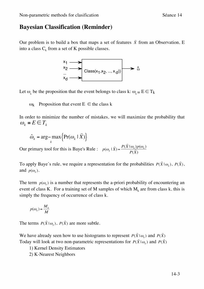
Bayesian Classification (Reminder) Our problem is to build a box that maps a set of features

!

! X from an Observation, E

into a class Ck from a set of K possible classes.

Class(x1,x2, ..., x d)} !̂

x1x2...xd

Let ωk be the proposition that the event belongs to class k: ωk = E ∈ Tk

ωk Proposition that event E ∈ the class k In order to minimize the number of mistakes, we will maximize the probability that

!

"k # E $ Tk

!

ˆ " k = arg#maxk

Pr("k |! X ){ }

Our primary tool for this is Baye's Rule :

!

p("k |! X ) =

P(! X |"k )p("k )

P(! X )

To apply Baye’s rule, we require a representation for the probabilities

!

P(! X |"k ),

!

P(! X ),

and

!

p("k ). The term

!

p("k ) is a number that represents the a-priori probability of encountering an event of class K. For a training set of M samples of which Mk are from class k, this is simply the frequency of occurrence of class k.

!

p("k ) =Mk

M

The terms

!

P(! X |"k ),

!

P(! X ) are more subtle.

We have already seen how to use histograms to represent

!

P(! X |"k ) and

!

P(! X )

Today will look at two non-parametric representations for

!

P(! X |"k ) and

!

P(! X )

1) Kernel Density Estimators 2) K-Nearest Neighbors

Non-parametric methods for clasification Séance 14

14-4

Variable size histogram cells (from lesson 13) Suppose that we have a D-dimensional feature vector

!

! X with each feature quantized

to N possible values, and suppose that we represent

!

P(! X ) as a D-dimensional

histogram h(

!

! X ). Let us fill the histogram with M training samples

!

{! X m} .

Let us define the volume of each cell as 1. Then the volume of the entire space is Q=ND. The volume for any block of V cells is V. In lesson 13 we observed that if the quantity of training data is too small, ie M < 8Q we can combine adjacent cells so as to amass enough data for a reasonable estimate. Suppose we merge V adjacent cells such that we obtain a combined sum of P.

!

P = h! X "V# (

! X )

The probability

!

p(! X ) for

!

! X "V is

!

p(! X m "V ) =

PMV

This is typically written as:

!

p(! X ) =

PMV

We can use this equation to develop two alternative non-parametric methods. Fix V and determine P => Kernel density estimator. Fix P and determine V => K nearest neighbors. (note in most developments the symbol “K” is used for the sum the cells. This conflicts with the use of K for the number of classes. Thus we substitute the symbol P for the sum of adjacent cells).

Non-parametric methods for clasification Séance 14

14-5

Kernel Density Estimators For a Kernel density estimator, we will represent each data point with a kernel function

!

k(! X ).

Popular Kernel functions are a hypercube centered of side w a sphere of radius w a Gaussian of standard deviation w. We can define the function for the hypercube as

!

k(! u ) =1 if ud "1 2 for all d =1,...,D0 otherwise

# $ %

This is called a Parzen window. For a position

!

! X , the total number of points lying with a cube with side w will be:

!

P = k! X "! X m

w#

$ %

&

' (

m=1

M

)

The volume of the cube

!

V =1wD .

Thus the probability

!

p(! X ) =

PMV

=1

MwD k! X "! X m

w#

$ %

&

' (

m=1

M

)

The Hypercube has a discontinuity at the boundaries. We can soften this using a triangular function evaluated on a sphere.

!

k(! u ) =1" 2 ! u if ! u #1 2 for all d =1,...,D

0 otherwise

$ % &

Even better is to use a Gaussian kernel with standard deviation σ = w.

!

k(! u ) = e"12

! u 2

w2

Non-parametric methods for clasification Séance 14

14-6

We can note that the volume is

!

V = (2")D /2wD

In this case

!

p(! X ) =

PMV

=1

M (2")D /2wD k! X #! X m( )

m=1

M

$

This corresponds to placing a Gaussian over each point and summing the Gaussians. In fact, we can choose any function

!

k(! u ) as kernel, provided that

!

k(! u ) " 0 and

!

k(! u )d! u " =1 The Gaussian Kernel tends to be popular for Machine Learning.

Non-parametric methods for clasification Séance 14

14-7

K Nearest Neighbors For K nearest neighbors, we hold P constant and vary V. (We have used the symbol P for the number of neighbors, rather than K to avoid confusion with the number of classes). As each data samples,

!

! X m , arrives, we construct a tree structure (such as a KD Tree)

that allows us to easily find the P nearest neighbors for any point . To compute

!

p(! X ) we need the volume of a sphere of radius ||

!

! X "! X K || in D

dimensions. This is:

!

V = CD

! X "! X K

D where

!

CD = +"D2

#D2

+1$

% &

'

( )

Where for positive integer n, Γ(n) = (n-1)!

and more generally for complex z,

!

"(z) = e# t0

$

% t z#1dt

For odd D, use a table to determine

!

"D2

+1#

$ %

&

' (

Then as before:

!

p(! X ) =

PMV

Non-parametric methods for clasification Séance 14

14-8

Probability Density Functions The alternative to a non-parametric representation is to use a function to represent

!

P(! X |"k ) and

!

P(! X ). Such a function is referred to as a “Probability Density Function”

or PDF. A probability density function of a continuous random variable is a function that describes the relative likelihood for this random variable to occur at a given point in the observation space. Definition: "Likelihood" is a relative measure of belief or certainty. Note: Likelihood is not probability. We will use the "likelihood" to determine the parameters for parametric models of probability density functions. To do this, we first need to define probability density functions. A probability density function, p(

!

! X ), is a function of a continuous variable or vector,

!

! X "RD , of random variables such that : 1)

!

! X is a vector of D real valued random variables with values between [–∞, ∞]

2)

!

p(! X )

"#

#

$ =1

Note that, p(

!

! X ) is NOT a number but a continuous function. To obtain a probability

we must integrate over some volume V of the D dimensional feature space.

!

P(! X "V ) = p(

! X )d! X

V#

This integral gives a number that can be used as a probability. In the case of D=1, the probability that X is within the interval [A, B] is

!

p(X " A,B[ ]) = p(x)dxA

B

#

Consider

!

p("k |! X ) =

p(! X |"k )p(! X )

p("k )

While

!

p(! X ) and

!

p(! X |"k ) are NOT numbers, their ratio IS a number.

The ratio of two pdfs gives a probability value!