Non-Markovian dynamics of an open quantum...

Non-Markovian dynamics of an open quantum system in fermionic environments

J. Q. You Department of Physics, Fudan University, Shanghai,

and Beijing Computational Science Research Center Beijingand Beijing Computational Science Research Center, Beijing

Mi Chen (PhD student at Fudan)

The Workshop on Correlations and Coherence in Quantum Systems Evora, Portugal, 8-12 October, 2012

Supported by the National Natural Science Foundation of China and the National Basic Research Program of China (973 Program)

Outline

• Open quantum systems and the master equation formalism: Non-Markov vs. Markov

• Non-Markovian quantum state diffusion (QSD) in a bosonic bath: Some exactly solvable modelsbosonic bath: Some exactly solvable models

• Non-Markovian QSD in fermionic environments

• Summary and outlook

What is an open quantum system?

Open system Environment Closed system

System plus environment framework

How to describe its dynamics?

Considered system Noise

Reduced density operator: { }sys env tot( ) ( )t Tr tρ ρ=

Non-Markov or Markov

Non-Markov is the rule, Markov is the exception (N. G. van Kampen)

Non-Markov vs. Markov

• Non-Markovian dynamics (memory environment):

The time evolution of the system’s state depends on its history.

M k i ti ( l i t)

sys 0

( ) [ , ( )] ( , ) ( )tt i H t t s s ds

tρ ρ κ ρ∂

= − +∂ ∫h

• Markov approximation (memoryless environment):

The reservoir is assumed to be of a broadband spectrum, so as to have a correlation time (memory time) much shorter than the dynamical (evolution) time of the considered system.

Replace ( ) by ( ) Lindblad form:s tρ ρ ⇒

† †sys[ , ] ([ , ] [ , ])

2t

t t ti H L L L L

tρ ρ ρ ρ∂ Γ

= − + +∂ h

Master equation under Born-Markov approximation

Born approximation (2nd-order approximation): Weak interaction

Typical assumption: (0) (0) (0)tot sys envρ ρ ρ= ⊗

int int int2 0

( ) 1[ , ( )] ' [ ( ),[ ( '), ( ')]]t

sys env

t i H t dt H t H t tt

ρ ρ ρ∂= − −

∂ ∫h h

Markov approximation: int intReplace ( ') by ( )t tρ ρ

int int int2 0

( ) 1[ , ( )] ' [ ( ),[ ( '), ( )]]t

sys env

t i H t dt H t H t tt

ρ ρ ρ∂= − −

∂ ∫h h

H. Carmichael, An open systems approach to quantum optics (Springer 1993)

One can use it to derive a non-Markovian master equation, but this method is perturbative (i.e., it applies to a weak system-bath coupling).

Two non-pertutbative methods for non-Markovian dynamics

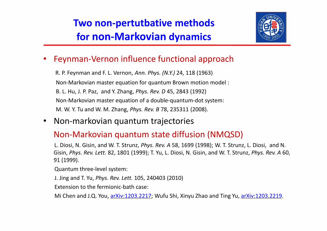
• Feynman-Vernon influence functional approach R. P. Feynman and F. L. Vernon, Ann. Phys. (N.Y.) 24, 118 (1963)

Non-Markovian master equation for quantum Brown motion model :

B. L. Hu, J. P. Paz, and Y. Zhang, Phys. Rev. D 45, 2843 (1992)

Non-Markovian master equation of a double-quantum-dot system:

M. W. Y. Tu and W. M. Zhang, Phys. Rev. B 78, 235311 (2008).

• Non-markovian quantum trajectories

Non-Markovian quantum state diffusion (NMQSD)L. Diosi, N. Gisin, and W. T. Strunz, Phys. Rev. A 58, 1699 (1998); W. T. Strunz, L. Diosi, and N. Gisin, Phys. Rev. Lett. 82, 1801 (1999); T. Yu, L. Diosi, N. Gisin, and W. T. Strunz, Phys. Rev. A 60, 91 (1999).

Quantum three-level system:

J. Jing and T. Yu, Phys. Rev. Lett. 105, 240403 (2010)

Extension to the fermionic-bath case:

Mi Chen and J.Q. You, arXiv:1203.2217; Wufu Shi, Xinyu Zhao and Ting Yu, arXiv:1203.2219.

Outline


• Non-Markovian quantum state diffusion (QSD) in a bosonic bath: Some exactly solvable modelsbosonic bath: Some exactly solvable models



Some exactly solvable models

*(tot sys kk

H H g L= +∑ † † )k k kk

b g Lb+ +∑ †k k kb bω

* *( ) [ ( , *)] ( *)t sys t tz iH Lz L O t z ztψ ψ+∂

= − + +∂

* *( ) ( ) ( )t

O t z t s O t s z dsα= −∫

*{ ( ) ( ) }t t tz zρ ψ ψ≡Μ

Stochastic Schrödinger equation (Diosi-Gisin-Strunz equation)

Total Hamiltonian:

( )( ) ( ) i t st s J e dωα ω ω∞ − −= ∫

• Spin-boson pure dephasing model

2sys zH ωσ= zL σ= *( , , )O t s z L=

• Spin-boson dissipative model

2sys zH ωσ= L σ−= *( , , ) ( , )O t s z f t s σ−=

0( , ) [ ( ') ( , ') '] ( , )

tf t s i t s f t s ds f t st

ω α∂= + −

∂ ∫ ( , ) 1f t t =

0( , ) ( ) ( , , )O t z t s O t s z dsα= −∫ ( )

0( ) ( )t s J e dα ω ω− = ∫

• Damped harmonic oscillator model

Some exactly solvable models

†sysH a aω= L a= *( , , ) ( , )O t s z f t s a=

0( , ) [ ( ') ( , ') '] ( , )

tf t s i t s f t s ds f t st

ω α∂= + −

∂ ∫ ( , ) 1f t t =

• Quantum Brown motion model2

2 212 2syspH m qm

ω= + L q=

*'0

( , , ) ( , ) ( , ) ( , , ') 't

sO t s z f t s q g t s p i j t s s z ds= + − ∫Exact non-Markovian master equation

2( ) ( )[ , ] [ , ] [ ,{ , }] ( )[ ,[ , ]] ( )[ ,[ , ]]2 2t sys t t t t ta t b ti H q q p c t q p d t q q

t i iρ ρ ρ ρ ρ ρ∂

= − + + + −∂

W. T. Strunz and T. Yu, Phys. Rev. A 69, 052115 (2004).B. L. Hu et. al., Phys. Rev. D 45, 2843 (1992);

Outline


• Non-Markovian quantum state diffusion (QSD) in a bosonicbath: Some exactly solvable models


Solid-state quantum circuits (see, e.g., JQY and Nori, Nature 474, 589-597 (2011) ; Xiang, Ashhab, JQY and Nori, arXiv: 1204.2137, to appear in Rev. Mod. Phys.)

Fermionic baths: Electric leads, background charge fluctuations, ……


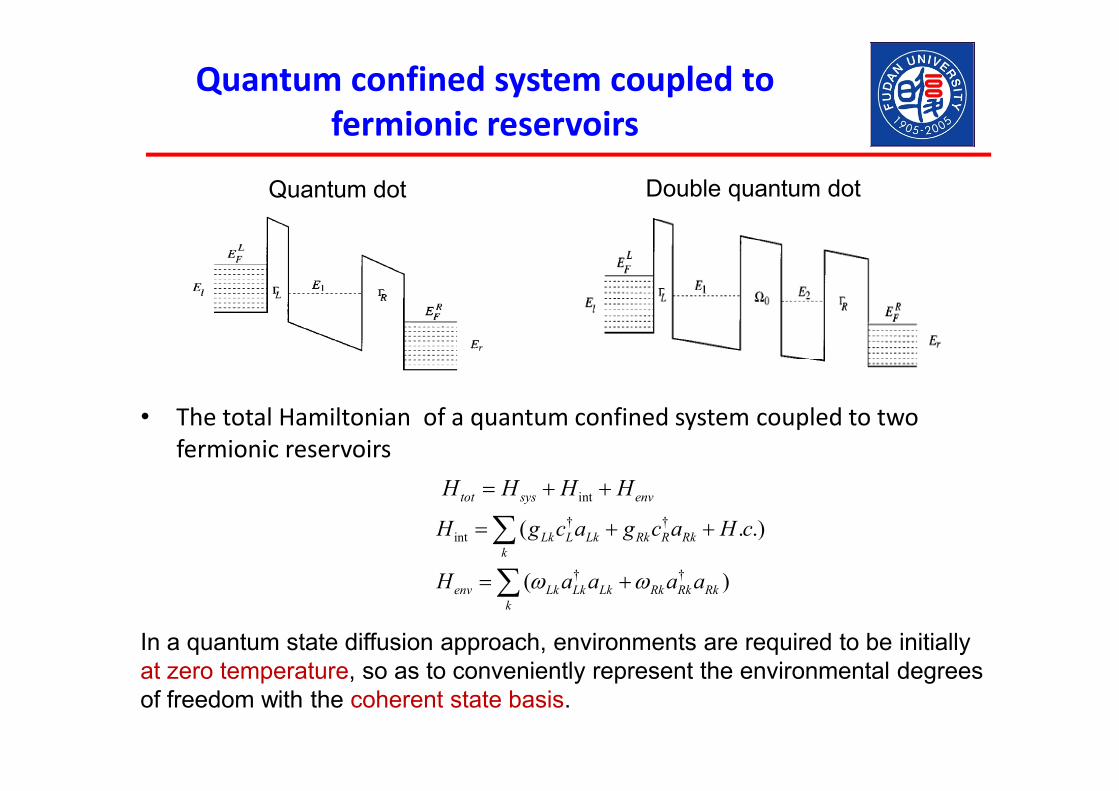
Quantum confined system coupled to fermionic reservoirs

Quantum dot Double quantum dot

• The total Hamiltonian of a quantum confined system coupled to two fermionic reservoirs

inttot sys envH H H H= + +

† †( )env Lk Lk Lk Rk Rk Rkk

H a a a aω ω= +∑

† †int ( . .)Lk L Lk Rk R Rk

kH g c a g c a H c= + +∑

In a quantum state diffusion approach, environments are required to be initially at zero temperature, so as to conveniently represent the environmental degrees of freedom with the coherent state basis.

Bogoliubov transformation: Converting a nonzero- to a zero-temperature problem

† † †( . .)tot sys k k k k k k k kk k k

H H g c a H c a a b bλ λ λ λ λ λ λ λ λλ λ λ

ω ω= + + + +∑ ∑ ∑

As for environments initially with a nonzero temperature, one can map the nonzero-temperature density operator to a zero-temperature density operator using a Bogoliubov transformation [T. Yu, Phys. Rev. A 69, 062107 (2004)].

By including the part involving holes in the electric leads, the total Hamiltonian can be written as

Performing Bogoliubov transformation for fermionic operators:

†1 k kk k ka n d n eλ λλ λ λ= − − †1 k kk k kb n e n dλ λλ λ λ= − +

† *' 1 ( . .) ( . .)k ktot sys k k k kk k

H H n g c d H c n g c e H cλ λλ λ λ λ λ λλ λ

= + − + + + +∑ ∑ † †k k k k k k

k kd d e eλ λ λ λ λ λ

λ λ

ω ω+∑ ∑

† *' ( ) ( 1 . .)k ki t i tk ktot sys k k k k

kH t H n g c d e n g c e e H cλ λω ω

λ λλ λ λ λ λ λλ

−= + − + +∑

The fermionic baths with nonzero initial temperatures are mapped to virtualfermionic baths with zero initial temperature.

Fermionic coherent states representation

0 0 0ψΨ = ⊗• Initial condition 0 0 0d eλ λ λ

= ⊗ ⊗

0 0kdλ = 0 0keλ =

• Fermionic coherent state basis for the environments†

0k kkz d

k kz z e λ λ

λ λ

−∑= ⊗ =†

0k kkw e

k kw w e λ λ

λ λ

−∑= ⊗ = zw z wλ λ λ= ⊗ ⊗

G i blGrassmann variables ,k kz wλ λ

*k kd zw z zwλ λ= †

*kk

d zw zwzλλ

∂=∂

• In the coherent state representation *( , )t tz w zwψ ≡ Ψ

( )t tot tiH tt∂

Ψ = − Ψ∂

*( , ) ( )t tot tz w i zw H ttψ∂

= − Ψ∂

Use the following equations:*

k ke zw w zwλ λ= †*kk

e zw zwwλλ

∂=∂

*

* * *

( )( )k k

z s dsz z z s

λ

λ λ λ

δδ

∂∂=

∂ ∂∫*

* * *

( )( )k k

w s dsw w w s

λ

λ λ λ

δδ

∂∂=

∂ ∂∫ (chain rules)

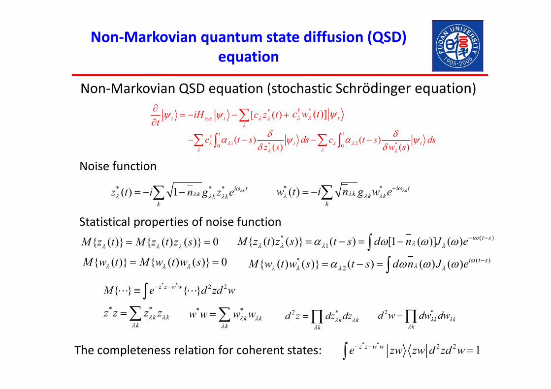
Non-Markovian quantum state diffusion (QSD) equation

Non-Markovian QSD equation (stochastic Schrödinger equation)*[ ( )t sys tiH c z t

t λ λλ

ψ ψ∂= − − +

∂ ∑†

1 2* *0 0( ) ( )

( ) ( )t t

t tc t s ds c t s dsz s w sλ λ λ λ

λ λλ λ

δ δα ψ α ψδ δ

− − − −∑ ∑∫ ∫

† * ( )] tc w tλ λ ψ

Noise function

* * *( ) 1 ki tk k kz t i n g z e λωλλ λ λ= − −∑ * *( ) ki t

k k kw t i n g w e λωλλ λ λ

−= − ∑( ) 1 k k kk

z t i n g z eλλ λ λ∑ ( ) k k kk

w t i n g w eλλ λ λ∑

Statistical properties of noise function* ( )

1{ ( ) ( )} ( ) [1 ( )] ( ) i t sM z t z s t s d n J e ωλλ λ λ λα ω ω ω − −= − = −∫{ ( )} { ( ) ( )} 0M z t M z t z sλ λ λ= =

{ ( )} { ( ) ( )} 0M w t M w t w sλ λ λ= = * ( )2{ ( ) ( )} ( ) ( ) ( ) i t sM w t w s t s d n J e ω

λλ λ λ λα ω ω ω −= − = ∫* * 2 2{ } { }z z w wM e d zd w− −≡ ∫L L

* *k k

kz z z zλ λ

λ

= ∑ * *k k

kw w w wλ λ

λ

= ∑ 2 *k k

k

d z dz dzλ λλ

=∏ 2 *k k

k

d w dw dwλ λλ

=∏

The completeness relation for coherent states:* * 2 2 1z z w we zw zw d zd w− − =∫

The O-operator and its equation of motion

• Like the Diosi-Gisin-Strunz equation in the bosonic-bath case, we introduce the O-operators:

Non-Markovian QSD equation (stochastic Schrödinger equation)*[ ( )t sys tiH c z t

t λ λλ

ψ ψ∂= − − +

∂ ∑†

1 2* *0 0( ) ( )

( ) ( )t t

t tc t s ds c t s dsz s w sλ λ λ λ

λ λλ λ

δ δα ψ α ψδ δ

− − − −∑ ∑∫ ∫

† * ( )] tc w tλ λ ψ

introduce the O operators:

* * * * * *1* ( , ) ( , , , ) ( , )

( ) t tz w O t s z w z wz s λλ

δ ψ ψδ

=

* * * * * *2* ( , ) ( , , , ) ( , )

( ) t tz w O t s z w z ww s λλ

δ ψ ψδ

=

* *1( , , , )O t t z w cλ λ=

* *2( , , , )O t t z wλ = †cλ

† * *'1 '2' ' ' ' ' '

' '

[ ( ), ] ({ , } ( ) { , } ( ))nsys n n n n

O iH c O c O O Q c O z t c O w ttλ

λ λλ λ λ λ λ λ λ λ λλ λ

+∂= − − + + + +

∂ ∑ ∑1 1 2 2† †L R L R

n L R L Rn n n n

O O O OQ c c c cδ δ δ δδ δ δ δ

= + + +Λ Λ Λ Λ

*1 ( )z sλΛ = *

2 ( )w sλΛ =

• Equation of motion for the O-operators:

Non-Markovian master equation

• Stochastic projection operator

* *( , ) ( , )t t tP z w z wψ ψ≡ − − { }t tM Pρ =

Stochastic reconstruction of the reduced density operator:

* * * * 2 2 * *( , ) ( , ) { ( , ) ( , ) }z z w wt env t t t t t tTr e z w z w d zd w M z w z wρ ψ ψ ψ ψ− −= Ψ Ψ = − − ≡ − −∫

• Non-Markovian master equation † † * *

1 1[ , ] ([ , { ( , , )}] [ , { ( , , ) }]t sys t t ti H c PO t z w c O t z w Pt

λ λλ λλ

ρ ρ∂= − + Μ − − − Μ

∂ ∑* *

2[ , { ( , , ) }]tc O t z w Pλλ− Μ††

2[ , { ( , , )}]tc PO t z wλλ+ Μ − −

• Markov limit 1( ) [1 ] ( )t s n t sλλ λα δ− → − Γ − 2 ( ) ( )t s n t sλλ λα δ− → Γ −

† † † † † †[ , ] [ (2 ) (1 )(2 )]2t sys t t t t t t ti H n c c c c c c n c c c c c c

tλ

λ λλ λ λ λ λ λ λ λ λ λ λ λλ

ρ ρ ρ ρ ρ ρ ρ ρΓ∂= − + − − + − − −

∂ ∑

Generally, it is complex, but can have a simple form for a given system.

Applications: (1) Single quantum dot

• Single quantum dot

†0sysH c cω= L Rc c c= =

* * * *1 1 10( , , , ) ( , ) ( , , ')[ ( ') ( ')] '

t

L RO t s z w f t s c q t s s w s w s dsλ = + +∫* *

2 2( , , , ) ( , )O t s z w f t sλ = † * *20( , , ')[ ( ') ( ')] '

t

L Rc q t s s z s z s ds+ +∫

• O-operators



H a a a aω ω= +∑† †

int ( . .)Lk L Lk Rk R Rkk

H g c a g c a H c= + +∑

Strong Coulomb blockade:

Constraint: Only one electron is allowed in the single quantum dot

U → ∞


∂

• Exact non-Markovian master equation

Final condition at :

with time-dependent rates:

† † *1 2 1[ , ] ( )[ , ] ( )[ , ] ( )t sys t t ti H t c c t c c t

tρ ρ ρ ρ∂

= − + Γ +Γ −Γ∂

† *2[ , ] ( )tc c tρ −Γ †[ , ]tc cρ

1 20( ) [ ( ) ( , ) ( ) ( , )]

t

j j jt t s A t s t s B t s dsα αΓ = − − −∫ ( ) ( ) ( )j L j R jt s t s t sα α α− = − + −

0 0( ) ( , ) ( ') ( , ') ' ( , )

s

j ji A t s s s A t s ds U t ss

ω β∂− + − =

∂ ∫

0 0( ) ( , ) ( ') ( , ') ' ( , )

s

j ji B t s s s B t s ds V t ss

ω β∂− + − =

∂ ∫

20( , ) ( ) ( , ') '

tU t s t s h t s dsα= −∫

10( , ) ( ) ( , ') '

tV t s t s h t s dsα= −∫

1 2( ') ( ' ) ( ')s s s s s sβ α α− = − + −0( ) ( , ) ( ') ( , ') ' 0t

si h t s t s h t s ds

sω β∂

− − − =∂ ∫

s t= 1 1( , ) ( , ) ( , ) 1A t t B t t h t t= = = 2 2( , ) ( , ) 0A t t B t t= =


† † *1 2 1[ , ] ( )[ , ] ( )[ , ] ( )t sys t t ti H t c c t c c t

tρ ρ ρ ρ∂

= − +Γ +Γ −Γ∂

† *2[ , ] ( )tc c tρ −Γ †[ , ]tc cρ

• Exact non-Markovian master equation


Markov limit:

1 0 01 1( ) [1 ( )] [1 ( )]2 2

L RL Rt n nω ωΓ → − Γ + − Γ

2 0 01 1( ) ( ) ( )2 2

L RL Rt n nω ωΓ → − Γ − Γ

Master equation in the Lindblad form:


tλ


ρ ρ ρ ρ ρ ρ ρ ρΓ∂= − + − − + − − −

∂ ∑

00 00 11L Rρ ρ ρ= −Γ +Γ&

11 00 11L Rρ ρ ρ= Γ −Γ&

10 0 10[ ]L Riρ ω ρ= − + Γ + Γ&

S. A. Gurvitz and Ya. S. Prager, Phys. Rev. B 53, 15932 (1996)

0 empty dot state

1 occupied dot state

Large bias limit: 0L Rμ ω μ> > 0( ) 1Ln ω = 0( ) 0Rn ω =Zero temperature:

q

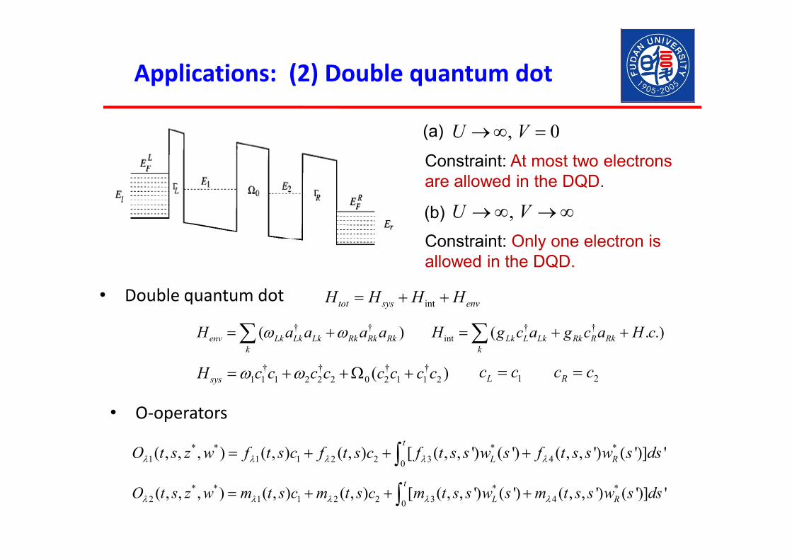
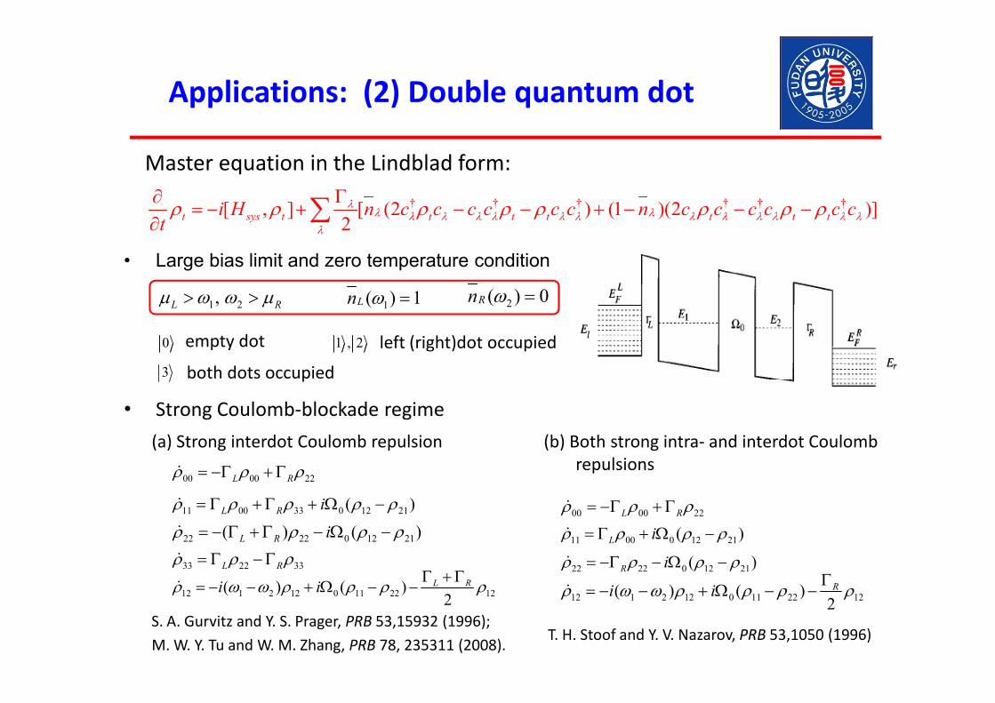
Applications: (2) Double quantum dot

, 0U V→∞ =

, U V→∞ →∞

Constraint: At most two electrons are allowed in the DQD.

Constraint: Only one electron is allowed in the DQD.

(a)

(b)

• Double quantum dot

† † † †1 1 1 2 2 2 0 2 1 1 2( )sysH c c c c c c c cω ω= + +Ω + 1Lc c= 2Rc c=

* * * *1 1 1 2 2 3 40( , , , ) ( , ) ( , ) [ ( , , ') ( ') ( , , ') ( ')] '

t

L RO t s z w f t s c f t s c f t s s w s f t s s w s dsλ λ λ λ λ= + + +∫* * * *

2 1 1 2 2 3 40( , , , ) ( , ) ( , ) [ ( , , ') ( ') ( , , ') ( ')] '

t

L RO t s z w m t s c m t s c m t s s w s m t s s w s dsλ λ λ λ λ= + + +∫



H a a a aω ω= +∑ † †int ( . .)Lk L Lk Rk R Rk

kH g c a g c a H c= + +∑

• O-operators


Exact non-Markovian master equation

† † † †1 1 1 2 1 1 3 1 2 4 1 2[ , ] ( )[ , ] ( )[ , ] ( )[ , ] ( )[ , ]t sys t L t L t L t L ti H t c c t c c t c c t c c

tρ ρ ρ ρ ρ ρ∂

= − +Γ +Γ +Γ +Γ∂ † † † †( )[ ] ( )[ ] ( )[ ] ( )[ ]t t t tΓ Γ Γ Γ† † † †

1 2 1 2 2 1 3 2 2 4 2 2( )[ , ] ( )[ , ] ( )[ , ] ( )[ , ]R t R t R t R tt c c t c c t c c t c cρ ρ ρ ρ+Γ +Γ +Γ +Γ*

1( )L t−Γ † *1 1 2[ , ] ( )t Lc c tρ −Γ † *

1 1 3[ , ] ( )t Lc c tρ −Γ † *1 2 4[ , ] ( )t Lc c tρ −Γ †

1 2[ , ]tc cρ*

1( )R t−Γ † *2 1 2[ , ] ( )t Rc c tρ −Γ † *

2 1 3[ , ] ( )t Rc c tρ −Γ † *2 2 4[ , ] ( )t Rc c tρ −Γ †

2 2[ , ]tc cρ

1 20( ) [ ( ) ( , ) ( ) ( , )]

t

j j jt t s A t s t s B t s dsλ λ λ λ λα αΓ = − − −∫

with time-dependent rates

( , )jA t sλ ( , )jB t sλ satisfy a set of integro-differential equations, with final conditions

1 3 2 4( , ) ( , ) ( , ) ( , ) 1L R L RA t t A t t B t t B t t= = = =

( , ) ( , ) 0j jA t t B t tλ λ= = for other , jλ


Markov limit:1 1

1 11( ) [1 ( )]2

LL Lt n ωΓ = − Γ 2 11( ) ( )2

LL Lt n ωΓ = − Γ

3 21( ) [1 ( )]2

RR Rt n ωΓ = − Γ 4 21( ) ( )2

RR Rt n ωΓ = − Γ

1 2 3 4( ) ( ) ( ) ( ) 0R R L Lt t t tΓ = Γ = Γ = Γ =


tλ


ρ ρ ρ ρ ρ ρ ρ ρΓ∂= − + − − + − − −

∂ ∑





tλ


ρ ρ ρ ρ ρ ρ ρ ρΓ∂= − + − − + − − −

∂ ∑

1 2, L Rμ ω ω μ> > 1( ) 1Ln ω = 2( ) 0Rn ω =

empty dot 1 , 20 left (right)dot occupied

• Large bias limit and zero temperature condition

00 00 22L Rρ ρ ρ= −Γ +Γ&

11 00 33 0 12 21( )L R iρ ρ ρ ρ ρ= Γ +Γ + Ω −&

22 22 0 12 21( ) ( )L R iρ ρ ρ ρ= − Γ +Γ − Ω −&

12 1 2 12 0 11 22 12( ) ( )2

L Ri iρ ω ω ρ ρ ρ ρΓ +Γ= − − + Ω − −&

33 22 33L Rρ ρ ρ= Γ −Γ&

00 00 22L Rρ ρ ρ= −Γ +Γ&

11 00 0 12 21( )L iρ ρ ρ ρ= Γ + Ω −&

22 22 0 12 21( )R iρ ρ ρ ρ= −Γ − Ω −&

12 1 2 12 0 11 22 12( ) ( )2Ri iρ ω ω ρ ρ ρ ρΓ

= − − + Ω − −&

(b) Both strong intra- and interdot Coulomb repulsions

3 both dots occupied

S. A. Gurvitz and Y. S. Prager, PRB 53,15932 (1996);T. H. Stoof and Y. V. Nazarov, PRB 53,1050 (1996)

(a) Strong interdot Coulomb repulsion

• Strong Coulomb-blockade regime

M. W. Y. Tu and W. M. Zhang, PRB 78, 235311 (2008).

Summary and outlook

Summary

• Non-Markovian quantum state diffusion (QSD) approach is extended to deal with the fermionic environments.

• Non-Markovian master equation is derived.

• The approach is applied to single quantum dot and double quantum d h l d l i l d

Outlook

• Connection to Feynman-Vernon influence functional approach?

• Non-Markovian QSD for a spin environment?

• Non-Markovian QSD for the system nonlinearly coupled to either a bosonic or fermionic bath ?

dot, each coupled to two electric leads.

Non-Markovian dynamics of an open quantum...

Documents

Transcript of Non-Markovian dynamics of an open quantum...