Prediction of Restenosis After PCI with Contemporary Drug-Eluting Stents
Jahed Naghipoor
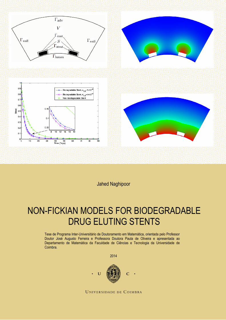
NON-FICKIAN MODELS FOR BIODEGRADABLE DRUG ELUTING STENTS
Tese de Programa Inter-Universitário de Doutoramento em Matemática, orientada pelo Professor Doutor José Augusto Ferreira e Professora Doutora Paula de Oliveira e apresentada ao Departamento de Matemática da Faculdade de Ciências e Tecnologia da Universidade de Coimbra.
2014

University of Coimbra
Doctoral Thesis
Non-Fickian Models forBiodegradable Drug Eluting
Stents
Author:
Jahed Naghipoor
Supervisors:
Professor Jose A. Ferreira
Professor Paula de Oliveira
Tese apresentada a Faculdade de Ciencias e Tecnologia da Universidade de
Coimbra, para a obtencao do grau de Doutor - Programa Inter-Universitario de
Doutoramento em Matematica
June 2014


iii
Abstract
Mathematical modeling and numerical simulation of cardiovascular drug de-
livery systems have become an effective tool to gain deeper insights in the phar-
macokinetics of therapeutic agents in cardiovascular diseases like atherosclerosis.
Drug Eluting Stents (DES) which are tiny expandable mesh tubes coated by a
polymer with dispersed drug, represent a major advance in the treatment of ob-
structed artery diseases.
The main objective of this thesis is to study a mathematical model that sim-
ulates ”in vivo” drug delivery from a biodegradable DES. To study the complete
problem of penetration of therapeutic agent from DES into the arterial wall, we
progressively address more complex models.
The first model, presented in Chapter 2, will describe with details, in a simple
two dimensional geometry, the biodegradation of polylactic acid (PLA), a material
of choice in the design of DES, that degrades due to the penetration of plasma
that breaks the polymer chains and reduces its molecular weight.
When drug diffuses from a polymer into a viscoelastic arterial wall, it is observed
that the process can not be completely described by Fick’s law of diffusion which
was proposed by Adolf Fick in 1855. The reason lies in the fact that as drug
diffuses into the arterial wall, it causes a deformation which induces a stress driven
diffusion that act as a barrier to the drug penetration. Thus a modified flux should
be considered, resulting from a sum of the Fickian flux and a non-Fickian flux.
To take into consideration this non-Fickian flux, we add a degree of complexity
to the first model, by introducing in Chapter 3 the stress response of the arterial
wall. It is a memory effect established by Maxwell-Wiechert model or Fung’s
quasilinear viscoelastic model.
To obtain a more realistic model of drug pharmacokinetics, the reversible na-
ture of binding, between the agent and immobilized sites in the arterial wall, is
considered in Chapter 4. The behavior of different families of drugs is compared.
Theoretical results concerning qualitative properties of the solutions and sta-
bility of the models are presented along the dissertation. From the numerical

iv
viewpoint some aspects of clinical importance such as the influence of elastic mod-
ulus of the arterial wall, the effect of biodegradation of PLA, the permeability of
the stent coating as well as the binding rates in the arterial wall will be addressed
in this thesis.
A software package, to simulate the models in this dissertation, has been de-
veloped using freeFEM++.
Keywords: Non-Fickian coupled model, cardiovascular drug delivery, drug
eluting stents, viscoelastic diffusion coefficient, numerical simulation.

v
Resumo
A modelacao matematica e a simulacao numerica do comportamento de sis-
temas de libertacao controlada de farmacos constituem instrumento centrais na
compreensao da farmacocinetica de agentes terapeuticos nas doencas cardiovascu-
lares, como por exemplo a aterosclerose. Os ”stents” com libertacao controlada
de farmaco1, que sao tubos metalicos revestidos por um polımero que contem um
farmaco disperso, constituem um tratamento de eleicao em caso de obstrucao de
vasos.
O objectivo central desta tese e o estudo analıtico e numerico de um mod-
elo matematico que descreva a libertacao de farmacos ”in vivo”, a partir de um
”stent” com revestimento biodegradavel. Para tal apresentamos ao longo da dis-
sertacao modelos progressivamente mais complexos, que culminam num sistema
que descreve a biodegradacao do polımero mas tambem propriedades dos tecidos
vasculares como a viscoelasticidade e a ocorrencia de afinidades entre o farrmaco
e o tecido vascular.
O primeiro modelo que estudamos, no Capıtulo 2, descreve com detalhe a in-
fluencia da biodegradacao do acido polilactico (PLA), que e um dos polımeros
mais usados no revestimento de stents. A degradacao ocorre devido a penetracao
do plasma no stent com a consequente quebra das cadeias do polımero e a reducao
do seu peso molecular.
Quando o farmaco se difunde na parede vascular, que e viscoelastica, o processo
nao pode ser completamente descrito pela Lei de Fick, proposta por Adolf Fick
em 1855. A razao reside no facto de o farmaco, ao difundir-se na parede vascular,
causar uma deformacao, que induz uma resposta do polımero sob a forma de uma
resistencia a penetracao do agente terapeutico. No Capıtulo 3 o fluxo Fickiano,
considerado no modelo do Capıtulo 2, e entao modificado, pela introducao de um
”anti-fluxo” de origem viscoelastica.
Para obter uma descricao mais realista da farmacocinetica do agente terapeutico
na parede do vaso incluımos, no Capıtulo 4, a afinidade quımica entre o agente e o
tecido vivo. O comportamento de farmacos hidrofılicos e hidrofobicos e analisado.
1Drug Eluting Stents (DES) em lıngua inglesa

vi
Sao apresentados nesta dissertacao resultados teoricos relativos as propriedades
qualitativas das solucoes e a estabilidade dos modelos estudados. Do ponto de
vista numerico sao discutidos diferentes aspectos de importancia clınica, como a
influencia do modulo de Young da parede vascular, as propriedades de degradacao,
a permeabilidade do revestimento polimerico e a afinidade do farmaco com a parede
vascular.
Foi desenvolvida uma aplicacao computacional, utilizando o ”software” de livre
acesso freeFEM++, para simular o comportamento dos modelos estudados nesta
tese.
Palavras chave: Modelo acoplado nao Fickiano, libertacao controlada de farmacos
no sistema cardiovascular, ”stents” com libertacao controlada de farmaco, coefi-
ciente de difusao viscoelastico, simulacao numerica.
Contents vii
Acknowledgments
Completing my PhD degree is probably the most challenging activity of my life
thus far. The best moments of my doctoral journey have been shared with many
people. It has been a great privilege to spend four years in the Department of
Mathematics at University of Coimbra, and its members will always remain dear
to me.
My first and foremost debt of gratitude must go to my supervisors, Professor
Jose Augusto Ferreira and Professor Paula de Oliveira for making it possible to
work on such a fascinating subject in the framework of my PhD thesis. They pa-
tiently provided the vision, encouragement and advise necessary for me to proceed
through the doctorial program and complete my thesis.
I would like to thank Fundacao para a Ciencia e a Tecnologia (FCT) for the fi-
nancial support under the scholarship SFRH/BD/51167/2010. My grateful thanks
are extended to the Centro de Matematica da Universidade de Coimbra (CMUC)
for supporting me in scientific events.
A special thank goes to my family. Words cannot express how grateful I am to
my mother, father and siblings for their unbounded supports. I would also like to
thank all of my friends who supported me in writing, and incented me to strive
towards my goal. We had great moments together in Coimbra.
Last but not the least, I would like to express my heartfelt gratitude to my
darling wife, Atefeh, for her unconditional love and unwavering supports.


Contents
Abstract iii
Resumo v
Acknowledgments vii
Contents vii
List of Figures xi
List of Tables xiii
Abbreviations xv
Symbols xvii
1 Introduction and Problem Setting 11.1 Controlled drug delivery . . . . . . . . . . . . . . . . . . . . . . . . 21.2 Arterial system: structural compounds and diseases . . . . . . . . . 31.3 Cardiovascular stents . . . . . . . . . . . . . . . . . . . . . . . . . . 71.4 Mathematical models for coupled cardiovascular drug delivery . . . . 11
2 A Nonlinear Coupled Model 152.1 Description of the model . . . . . . . . . . . . . . . . . . . . . . . . 162.2 Qualitative behavior of the total mass . . . . . . . . . . . . . . . . . 212.3 Weak formulation of the coupled problems . . . . . . . . . . . . . . 232.4 Stability analysis . . . . . . . . . . . . . . . . . . . . . . . . . . . . 262.5 Finite dimensional approximation . . . . . . . . . . . . . . . . . . . 292.6 Full discrete IMEX problem . . . . . . . . . . . . . . . . . . . . . . 302.7 Numerical experiments . . . . . . . . . . . . . . . . . . . . . . . . . 31
3 A Non-Fickian Coupled Model 433.1 Description of the model . . . . . . . . . . . . . . . . . . . . . . . . 44
3.1.1 Chemical reactions . . . . . . . . . . . . . . . . . . . . . . . 453.1.2 Convection . . . . . . . . . . . . . . . . . . . . . . . . . . . . 463.1.3 Viscoelastic effects . . . . . . . . . . . . . . . . . . . . . . . 483.1.4 A reaction-diffusion-convection problem . . . . . . . . . . . . 50
3.2 Qualitative behavior of the total mass . . . . . . . . . . . . . . . . . 543.3 Weak formulation . . . . . . . . . . . . . . . . . . . . . . . . . . . 55
ix

Contents x
3.3.1 Porous media problem . . . . . . . . . . . . . . . . . . . . . 553.3.2 Convection-diffusion-reaction problem . . . . . . . . . . . . . 57
3.4 Finite dimensional approximation . . . . . . . . . . . . . . . . . . . 643.4.1 Discrete porous media problem . . . . . . . . . . . . . . . . . 653.4.2 Discrete convection-diffusion-reaction problem . . . . . . . . 65
3.5 Full discrete IMEX problem . . . . . . . . . . . . . . . . . . . . . . 663.6 Numerical simulations . . . . . . . . . . . . . . . . . . . . . . . . . 68
4 The Effect of Reversible Binding 814.1 Reversible binding reactions . . . . . . . . . . . . . . . . . . . . . . 814.2 Non-Fickian reaction-diffusion-convection system . . . . . . . . . . 834.3 Numerical experiments . . . . . . . . . . . . . . . . . . . . . . . . . 84
5 Conclusions and Future Work 915.1 Conclusions . . . . . . . . . . . . . . . . . . . . . . . . . . . . . . . 915.2 Future work . . . . . . . . . . . . . . . . . . . . . . . . . . . . . . . 92

List of Figures
1.1 Classical and controlled release . . . . . . . . . . . . . . . . . . . . 21.2 Layers of the arterial wall . . . . . . . . . . . . . . . . . . . . . . . 41.3 Atherosclerosis . . . . . . . . . . . . . . . . . . . . . . . . . . . . . 61.4 Balloon angioplasty . . . . . . . . . . . . . . . . . . . . . . . . . . . 71.5 Bare metal stent . . . . . . . . . . . . . . . . . . . . . . . . . . . . 81.6 Drug eluting stent implanted in the blood artery . . . . . . . . . . . 9
2.1 Polymeric stent S in contact with the vessel wall V. . . . . . . . . . 162.2 Schematic of the mathematical model for predicting degradation of
PLA and drug release . . . . . . . . . . . . . . . . . . . . . . . . . . 172.3 Triangulation in the stent and in the arterial wall. . . . . . . . . . . 312.4 Drug distribution in the coating and the arterial wall after 1 day. . 322.5 Drug distribution in the coating and the arterial wall after 7 days. . 322.6 Drug distribution in the coating and the arterial wall after 14 days. 322.7 Concentration of water in the coating after 1 day. . . . . . . . . . . 332.8 Concentration of water in the coating after 7 days. . . . . . . . . . 332.9 Concentration of water in the coating after 14 days. . . . . . . . . . 332.10 Concentration of PLA in the coating after 1 day. . . . . . . . . . . . 342.11 Concentration of PLA in the coating after 7 days. . . . . . . . . . . 342.12 Concentration of PLA in the coating after 14 days. . . . . . . . . . 342.13 Diffusion coefficient of the drug in the stent for different reaction
rates κ1,S. . . . . . . . . . . . . . . . . . . . . . . . . . . . . . . . . 352.14 Diffusion coefficient of the drug in the stent for different values of α. 362.15 Mass of water in the stent . . . . . . . . . . . . . . . . . . . . . . . 372.16 Mass of drug in the stent . . . . . . . . . . . . . . . . . . . . . . . . 372.17 Mass of lactic acid in the stent . . . . . . . . . . . . . . . . . . . . . 382.18 Mass of PLA in the stent . . . . . . . . . . . . . . . . . . . . . . . . 382.19 Mass of water in the stent for different reaction rates. . . . . . . . . 392.20 Mass of lactic acid in the stent for different reaction rates. . . . . . 402.21 Mass of drug in the stent for different reaction rates. . . . . . . . . 402.22 Mass of PLA in the stent for different reaction rates. . . . . . . . . 41
3.1 DES embedded in the arterial wall . . . . . . . . . . . . . . . . . . 443.2 Generalized Maxwell-Wiechert linear model . . . . . . . . . . . . . 493.3 Maxwell-Wiechert model with n = 1 . . . . . . . . . . . . . . . . . 503.4 Triangulations in the stent and in the vessel wall. . . . . . . . . . . 643.5 Velocity field and pressure drop in the stented arterial wall . . . . . 693.6 Drug distribution in the stented arterial wall during 6 months . . . 70
xi

List of Figures xii
3.7 Drug distribution in the stent after 1 day. . . . . . . . . . . . . . . 713.8 The flux of drug in the stent after 1 day. . . . . . . . . . . . . . . . 713.9 Evolution of masses of water, PLA and drug in the stent during 90
days. . . . . . . . . . . . . . . . . . . . . . . . . . . . . . . . . . . . 723.10 Evolution of the mass of drug in biodegradable stent versus non-
biodegradable stent. . . . . . . . . . . . . . . . . . . . . . . . . . . 733.11 Evolution of the drug mass in the arterial wall for short time . . . . 743.12 Evolution of the drug mass in the arterial wall for long time . . . . 743.13 Evolution of the drug mass in the arterial wall for different values
of Dσ . . . . . . . . . . . . . . . . . . . . . . . . . . . . . . . . . . . 753.14 Evolution of the drug mass in the arterial wall for different values
of Pc. . . . . . . . . . . . . . . . . . . . . . . . . . . . . . . . . . . . 763.15 Evolution of the drug mass in the arterial wall for different values
of κr for short time (Fung’s model). . . . . . . . . . . . . . . . . . . 783.16 Evolution of the drug mass in the arterial wall for different values
of κr for long time (Fung’s model). . . . . . . . . . . . . . . . . . . 79
4.1 Schematic representation of free drug, binding to a specific bindingsite and a specific drug-binding site complex. . . . . . . . . . . . . . 82
4.2 Distribution of heparin in the arterial wall in the models withoutbinding sites and with binding site . . . . . . . . . . . . . . . . . . 85
4.3 Evolution of the mass of heparin in the arterial wall with and with-out binding site . . . . . . . . . . . . . . . . . . . . . . . . . . . . . 86
4.4 Distribution of heparin and paclitaxel in the arterial wall . . . . . . 874.5 Evolution of masses of heparin and paclitaxel in the arterial wall . . 884.6 Evolution of the mass of free paclitaxel in the healthy and diseased
arterial wall during 30 days. . . . . . . . . . . . . . . . . . . . . . . 884.7 Evolution of the mass of bound paclitaxel in the healthy and dis-
eased arterial wall during 30 days. . . . . . . . . . . . . . . . . . . . 89
List of Tables
2.1 Notation for the concentrations . . . . . . . . . . . . . . . . . . . . 18
3.1 Notation for the concentrations . . . . . . . . . . . . . . . . . . . . 45
4.1 Properties of heparin and paclitaxel . . . . . . . . . . . . . . . . . . 84
xiii


Abbreviations
DES Drug Eluting Stent
BMS Bare Metal Stent
PLA PolyLactic Acid
PLGA PolyLactic-co-Glycolic Acid
QLV Quasi-Linear Viscoelastic
FEM Finite Element Method
VP Variational Problem
FEVP Finite Element Variational Problem
IC Initial Condition
BC Boundary Condition
IBC Interface Boundary Condition
IBVP Initial Boundary Value Problem
IMEX IMplicit EXplicit
xv


Symbols
Symbol Name Unit
κ1,S, κ2,S, κ1,V Reaction rate cm2
g.s
κu,V Association rate cm2
g.s
κb,S Dissociation rate 1s
MW Molecular weight gmol
α, β, γ Autocatalysis rate scm2
kS, kV Permeability cm2
µS, µV Viscosity gcm.s
Cm,S, CV , Cm,V Concentration gcm2
Dm,S, DV , Dm,V Diffusion coefficient cm2
s
γm,V Transference rate cms
Pc Transference rate cms
xvii


Chapter 1
Introduction and Problem Setting
In this thesis, we address the analytical and numerical study of the diffusion of
a drug from a biodegradable stent and its release into a viscoelastic artery. The
mathematical results established will be used to study the pharmacokinetics of
drug eluting from a stent into the arterial wall.
In Chapter 1, we introduce biomedical concepts concerning the cardiovascular
system and refer some treatments of cardiovascular diseases like atherosclerosis.
We also establish the basic concepts to answer to the following questions:
• How can mathematical modeling clarify the mechanisms underlying the car-
diovascular drug delivery systems?
• Why are drug eluting stents useful medical devices in cardiovascular drug
delivery systems?
• What are the influences of the mechanical properties of the arterial wall and
the affinities drug/vascular tissue, in the process of drug release by drug
eluting stents?
Section 1.1 is devoted to controlled drug delivery and its application in medicine.
In Section 1.2 we review the structure of the arterial system to study possible
treatments of atherosclerosis. In Section 1.3 we investigate the application of
cardiovascular stents (bare metal stents and drug eluting stents), their advantages
1

Chapter 1. Introduction and Problem Setting 2
and failures for the treatment of the atherosclerosis. Polymer’s degradation and
its application in the cardiovascular stents will be also studied in this section.
Mathematical models are briefly reviewed in Section 1.4.
1.1 Controlled drug delivery
Controlled drug delivery is the release of drug at a specified rate which is
determined by the demand of the living system organ or tissue over a specified
period of time ([43]). Since the sudden delivery of too much drug can be harmful
and the release of too little amount of drug may limit its effectiveness, the control
of the rate of drug release is a crucial issue.
Figure 1.1: Profile of drug concentration in traditional release (red) and con-trolled release (blue) ([43]).
Traditional delivery systems are characterized by immediate and uncontrolled
drug release kinetics. Accordingly, drug absorption is essentially controlled by
the body’s ability to assimilate the therapeutic molecule and thus, drug concen-
tration in different body tissues, typically undergoes an abrupt increase followed
by a similar decrease. As a consequence, it may happen that drug concentration

Chapter 1. Introduction and Problem Setting 3
dangerously approaches the toxic threshold to subsequently fall down below the
effective therapeutic level ([18]).
To predefine the performance of drug delivery systems, traditional delivery
systems, as for example simple pills, have been replaced by controlled drug delivery
systems (see Figure 1.1) to maintain drug concentration in target tissues at a
desired value as long as possible and to help to control both under and overdosing
([18, 43]).
In controlled drug delivery systems part of the drug dose is initially released
in order to rapidly get the drug effective therapeutic concentration. Then, drug
release kinetics follows a well defined behavior in order to supply the maintenance
dose, enabling the attainment of the desired drug concentration ([18]).
There is a huge literature in the field of controlled drug delivery. Some of these
studies have an experimental character, others are completed with mathematical
models. We mention without being exhaustive to [10, 12, 18, 22, 24, 35, 43].
1.2 Arterial system: structural compounds and diseases
The vasculature is a complex architecture of vessels that carry blood to and
from the different organs of the body. The blood vessels may be classified based
on their sizes, function and proximity to the heart. A vessel named Artery with
1 mm wall thickness and 4 mm lumen thickness is one of the thickest vessels of
the arterial system which tolerate a pressure profile varying from 80 mmHg to 120
mmHg in each cardiac cycle.
Arteries are roughly subdivided into two types: elastic and muscular. Elas-
tic arteries are located close to the heart, have relatively large diameters and are
regarded as elastic structures. Muscular arteries are smaller, located at the periph-
ery and are regarded as viscoelastic structures. Smaller arteries typically display
more pronounced viscoelastic behavior than arteries with large diameters.
In what follows, we mention a few structural components of the arterial wall
which are bio-mechanically relevant.
• Endothelial cells are cells in the arterial wall in direct contact with blood
flow that have negligible mechanical properties. Its main action is the pre-
vention of thrombosis (the formation of a blood clot) and the entry of blood

Chapter 1. Introduction and Problem Setting 4
borne bacteria into the vascular wall. It can regenerate itself when it is
injured;
• Elastin is a protein in connective tissue with high elastic properties and
low stiffness. It allows tissues to resume their shape after stretching or
contracting. It can stretch up to 60 percent and remain elastic to bear the
load under physiological conditions;
• Collagen is a tortuous, thick fiber component of vascular wall with high
stiffness. It is responsible for structural integrity of the vessel;
• Smooth muscle cell is a component that is responsible for active properties
of blood vessel wall;
• Ground substance is a component that acts like a glue to keep all arterial
components together.
Figure 1.2: Layers of the arterial wall (http://www.3fx.com/Our-Work/Medical-Illustration.aspx).
Arterial walls are mainly composed of the three distinct layers named intima,
media and adventitia (see Figure 1.2).
• Intima is the innermost layer of the artery and offers negligible mechanical
strength in the healthy young individuals. It consists of an endothelial cell
mono-layer that prevents blood, including platelets and other elements, from
adhering to the lumenal surface. The mechanical contribution of the intima
may become significant for aged arteries where the intima becomes thicker
and stiffer;

Chapter 1. Introduction and Problem Setting 5
• Heterogeneous media, the thickest layer of the artery, is composed by
elastin (24%), vascular smooth muscle cells (33%), collagen (37%) and ground
substances (6%). However, it behaves mechanically as a homogeneous ma-
terial. Due to the high content of smooth muscle cells, it is the media that
is responsible for the viscoelastic behavior of the arterial wall;
• Adventitia is composed of elastin (2%), ground substances (9%), fibroblast
(9%) and collagen fibers (78%). At very high strains, the adventitia changes
to a stiff tube which prevents the artery from overstretching and rupturing.
In the healthy young individuals, only the media and the adventitia are respon-
sible for the strength of the arterial wall and play significant mechanical roles by
carrying most of the stresses. At low strains (physiological pressures), it is chiefly
the media that determines the properties of the arterial wall.
Other layers of arterial wall are as follow.
• Endothelium, a thin layer of cells with thickness 2µm that lines the interior
surface of blood vessel and vessel forming, as an interface between circulating
blood and the rest of the arterial wall;
• Glycocalyx, a thin layer of macromolecules with thickness 100nm to cover
a plasma membrane of a single layer of endothelial cells;
• Internal elastic lamina, a layer of elastic tissue with thickness 2µm that
forms the outermost part of the intima of blood vessels. It separates intima
from media;
• External elastic lamina, a layer of elastic connective tissue lying imme-
diately outside the smooth muscle of the media of the artery. It separates
media from adventitia.
Cardiovascular diseases are among the leading causes of death in the industrialized
world. Although since the 1970s, cardiovascular mortality rates have declined in
many high-income countries, cardiovascular deaths have increased at a fast rate in
low-income and middle-income countries ([40]). Among all cardiovascular diseases,
atherosclerosis is the most common cardiovascular disease wherein some arteries
start thickening until they eventually occlude. This process normally happens
over a period of 50 to 60 years and seems to get particularly severe with age. In
some cases, it begins in early life making primary prevention efforts necessary from
childhood ([40]).

Chapter 1. Introduction and Problem Setting 6
Figure 1.3: Atherosclerosis (http://www.nmihi.com/a/atherosclerosis.htm).
This disease is characterized by intramural deposits of lipids and proliferation of
vascular smooth muscle cells. These changes are accompanied by loss of elasticity
of the vessel wall and narrowing of the vascular lumen. Coronary atherosclerosis
is clinically the most important aspect of atherosclerosis. As coronary arteries are
relatively narrow, atherosclerosis could seriously reduce the blood flow through
them. Initial and advanced atherosclerosis in the coronary artery are depicted in
Figure 1.3.
To face with the pathology of atherosclerosis, different treatments have been
developed during the years. The technology moves from invasive techniques to
more safe and non invasive techniques.
Balloon angioplasty as it is shown in Figure 1.4, is the first technique of me-
chanically widening narrowed or obstructed arteries caused by atherosclerosis. An
empty and collapsed balloon on a guide wire, known as a balloon catheter, is
passed into the narrowed locations and then inflated to a fixed size using water
pressures between 75 to 500 times of normal blood pressure. Inflated balloon di-
lates the blocked segment of the artery by compressing the atherosclerosis plaque
and stretching of the arterial wall.
Chapter 1. Introduction and Problem Setting 7
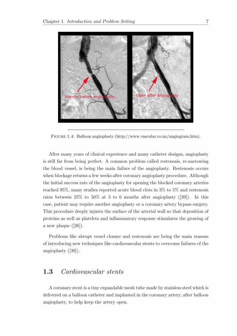
Figure 1.4: Balloon angioplasty (http://www.vascular.co.nz/angiogram.htm).
After many years of clinical experience and many catheter designs, angioplasty
is still far from being perfect. A common problem called restenosis, re-narrowing
the blood vessel, is being the main failure of the angioplasty. Restenosis occurs
when blockage returns a few weeks after coronary angioplasty procedure. Although
the initial success rate of the angioplasty for opening the blocked coronary arteries
reached 95%, many studies reported acute blood clots in 3% to 5% and restenosis
rates between 25% to 50% at 3 to 6 months after angioplasty ([39]). In this
case, patient may require another angioplasty or a coronary artery bypass surgery.
This procedure deeply injures the surface of the arterial wall so that deposition of
proteins as well as platelets and inflammatory response stimulates the growing of
a new plaque ([26]).
Problems like abrupt vessel closure and restenosis are being the main reasons
of introducing new techniques like cardiovascular stents to overcome failures of the
angioplasty ([39]).
1.3 Cardiovascular stents
A coronary stent is a tiny expandable mesh tube made by stainless steel which is
delivered on a balloon catheter and implanted in the coronary artery, after balloon
angioplasty, to help keep the artery open.

Chapter 1. Introduction and Problem Setting 8
After the plaque is compressed against the arterial wall, the stent is fully ex-
panded into position, thereby acting as a scaffold for the artery. The balloon is
then deflated and removed and the coronary stent is left behind in the patient’s
artery. This technique results in a treatment option that requires much less recov-
ery time when compared to balloon angioplasty ([39]).
In general, cardiovascular stents have two distinct and significant chronic fail-
ures:
• Immediately after deployment, thrombosis (acute blood clot) can occur due
to the thrombogenic aspect of the stent promoting a foreign body response.
This phenomena can be promptly treated with drug therapy;
• The other critical failure is in-stent restenosis which is the narrowing of a
stented coronary artery due to the development of neo-intimal hyperplasia
within the stent.
As it is already mentioned in Section 1.2, coronary balloon angioplasty is limited
by abrupt closure and high percent of restenosis. Due to mentioned failures, bare
metal stents (BMS) (Figure 1.5) were proposed to prevent these complications.
However, they are associated with restenosis rates of 25%− 30% and also around
20%−25% of bare metal stented arteries need a second procedure within 6 months.
The other failure of BMS is that due to their microstructural properties, metals
are not feasible materials to act as loadable drug carriers.
Figure 1.5: Bare metal stent (http://www.medgadget.com/2006/01).
All these drawbacks have encouraged significant efforts in the development of
new stent materials, either used in coatings or in stents completely made of poly-
meric materials. Drug eluting stent (DES) is one of these new stent materials.

Chapter 1. Introduction and Problem Setting 9
A DES is a stent that is coated by a polymer, containing an anti-proliferative
agent, which is released gradually over the course of weeks to months after insertion
of the stent. It will provide sustained inhibition of the neointimal proliferation as
a response of vascular injury.
In 2002− 2003, DES were approved by regulatory bodies in Europe and also in
the USA when initial studies showed a dramatic reduction in rates of restenosis
compared to BMS.
Figure 1.6: Drug eluting stent implanted in the blood artery(http://www.cxvascular.com/cn-latest-news/).
A DES (Figure 1.6) has three principal components: a stent platform (strut),
a polymer coating and a drug. The drug is contained within the polymer coating
and then diffuses into the arterial wall from the polymer source. The first DESs
were designed with nondegradable polymer coatings; however, some of the newer
DESs are manufactured with biodegradable polymer coatings ([43]).
Some benefits of DES are mentioned bellow:
• If a DES degrades in a controlled manner, the profile of released drug can
be predicted;
• The gradual softening of DES leads to a smooth transfer of the load from
the stent to the healing wall.
The primary pathophysiological mechanism of restenosis involves an exagger-
ated healing response of smooth muscle to vascular injury. In fact the injury made
by angioplasty induces smooth muscle cells to proliferate and migrate to subinti-
mal layer where the smooth muscle continue to migrate. These processes cause
neointimal mass to expand and gradually encroach on the coronary artery.

Chapter 1. Introduction and Problem Setting 10
It has been observed that smooth muscle cell derived from injuries of angio-
plasty show a higher migratory activity than cells made from primary injuries.
Injuries with higher aggressive smooth muscle cells will develop more restenosis
than an injury without such aggressive cells. Endothelial cells normally have some
inhibitors like nitric oxide and heparin sulfate to inhibit smooth muscle cell pro-
liferation. Their removal by angioplasty procedure contributes to a proliferative
environment leading to restenosis.
As it is mentioned earlier, new generation DES are made of biodegradable
polymers. A polymer is a large molecule made from many smaller units called
monomers. The mechanical properties of a polymer are determined by many
factors in addition to the monomer from which it is made. Properties such as
stiffness, strength and degradation time are affected by the number of monomers
within the chain (molecular weight) and the arrangement of the monomers. In
general, the greater the molecular weight (longer chain of monomers), the greater
strength and greater absorption time the polymer will have.
In DES, a polymeric material is used to coat the metallic struts, to serve as a
drug carrier and to regulate and control the elution of the drug. Numerous poly-
mers and co-polymers such as polylactic acid (PLA) and polylactic-co-glycolic acid
(PLGA) have been studied experimentally and empirical models of drug release
have been developed ([6, 8, 9]).
Studies to identify families of polymers that degrade predictably and disappear
over time have become increasingly important. In the case of polymers used in drug
eluting stents this aspect is crucial because the safe and predictable disappearance
is one of the key factors in evaluating their performance.
Biodegradable polymers have hydrolysable bonds, making hydrolysis the most
important mode of degradation. In biodegradable polymeric devices, the drug is
released by the degradation and dissolution of the polymeric matrix, or by the
cleavage of a covalent bond that binds the drug within the polymeric matrix.
Biodegradable polymers, however, are designed to slowly dissolve following im-
plantation. Biodegradable polymers used in drug delivery must induce no undesir-
able or harmful tissue responses, and the degradation products must be nontoxic.
PLA is the polymer most commonly used for the production of biodegradable
stents. Molecular weight of PLA is controlled by the quality of lactide used. The
less water the lactide contains, the purer the PLA, with a higher molecular weight.

Chapter 1. Introduction and Problem Setting 11
Pharmacological agents like dexamethasone, heparin, nitric oxide, paclitaxel
and sirolimus have been investigated to inhibit restenosis by angioplasty proce-
dure. These pharmacological agents have been used in stent coating in a number
of commercial drug eluting stents. Recently, two more drugs, everolimus and zo-
tarolimus, were added to the list of smooth muscle cell proliferation inhibitors used
in drug eluting stents. Everolimus is being clinically investigated by Abbott Vas-
cular, Santa Clara, CA, USA, with the XIENCE V TM everolimus eluting coronary
stent. The interesting fact about this drug is that it is used in conjunction with
a new biodegradable polymer coating and give promising results in initial clinical
studies.
In this dissertation, information from XIENCE V TM everolimus eluting coro-
nary stent investigated by Abbott Vascular is used to study the coronary drug
eluting stent.
1.4 Mathematical models for coupled cardiovascular drug
delivery
Mathematical modeling and numerical simulations of drug transport inside the
arterial wall help to understand the efficacy of the treatment and can provide
manufacturers with guidelines to optimize delivery from DES. During the last
years, a number of studies have proposed mathematical models for coupled drug
delivery in the cardiovascular tissues. We refer without being exhaustive to [2, 5,
24, 26, 33, 40, 43, 44, 46]. Most of these studies address the release of drug and
its numerical behavior in one dimension, while the viscoelasticity of the arterial
wall and the behavior of the biodegradable polymer are disregarded.
Pontrelli and de Monte ([31–33]) developed mathematical models for drug re-
lease through a DES in contact with the arterial wall as a coupled cardiovascular
drug delivery system. They analyzed numerically and analytically the drug release
from the coating into both a homogeneous mono-layer wall ([32]) and a heteroge-
neous multi-layered wall ([33]) in one dimension. Despite their interesting results,
the biodegradation process of the carrier polymer, the penetration of the biological
fluid into the coating and absorption of degraded polymer by the arterial wall have
not been taken into account.
Prabhu and Hossainy ([34]) developed a mathematical model to predict the
transport of drug with simultaneous degradation of the biodegradable polymer

Chapter 1. Introduction and Problem Setting 12
in the aqueous media. They have used a simplified wall-free condition, in which
the influence of the arterial wall is modeled through the coupling with a Robin
boundary condition. An important feature of this model, which differentiates it
from other models, is the reaction equations used to represent the polymer degra-
dation. It is assumed that a set of oligomers can be identified as one compartment,
characterized by a certain molecular weight range, for which their diffusion char-
acteristics and degradation kinetics can be considered to be identical. The authors
in [34] also consider that the diffusion coefficients depend on the concentration of
PLA.
The model presented in Chapter 2 extends to two dimensions the one dimen-
sional model proposed by Prabhu and Hossainy, and furthermore it uses a coupled
stent-wall system instead of a simplified wall-free condition. The model is based
on two sets of PDE’s: one represents the kinetics of the drug and the degradation
process in the stent and the other the kinetics of drug in the vessel wall. These
equations are based on Fick’s law and are described by∂CS∂t
+∇ · JS = FS,∂CV∂t
+∇ · JV = 0,(1.1)
where CS denotes a concentration (drug, PLA, oligomers, lactic acid and fluid) in
the stent coating, while CV represents the drug concentration in the arterial wall.
In system (1.1), Jj, j = S, V, represent Fickian mass fluxes in the stent and
in the arterial wall, respectively, whereas FS describes the degradation reactions.
The system is coupled with the initial, boundary and interface conditions.
The results presented in Chapter 2 are extensions of the results included in the
works:
• J. A. Ferreira, J. Naghipoor and P. de Oliveira, Numerical simulation of a
coupled cardiovascular drug delivery model, Proceedings of the 13th Interna-
tional Conference on Computational and Mathematical Methods in Science
and Engineering, CMMSE2013 (II), I. P. Hamilton and J. Vigo-Aguiar (ed-
itors), 642–653, 2013.
• J. A. Ferreira, J. Naghipoor and P. de Oliveira, Analytical and numerical
study of a coupled cardiovascular drug delivery model, Journal of Computa-
tional and Applied Mathematics, 275 (2015) 433–446.

Chapter 1. Introduction and Problem Setting 13
Arterial walls of the cardiovascular system are known to display a complex
mechanical response under physiological conditions. The coronary artery has dif-
ferent portions of the layers, which mainly consist of elastin that is responsible
for elasticity and smooth muscle cell and collagen in the media, which exhibit the
viscoelastic behavior of the artery ([27, 29]).
Experiments like creep tests have demonstrated that the vascular tissue is vis-
coelastic ([16, 27, 41]). It is accepted that in the presence of small vascular de-
formations, linear viscoelastic models will adequately predict the process of drug
penetration from stent into the arterial wall ([29]).
Classical Fickian diffusion equation does not account for the influence of vis-
coelasticity in the transport of molecules ([6, 10, 15, 16, 29]). From a mathematical
viewpoint, a non-Fickian reaction-diffusion equation characterized by a modified
flux could be an appropriate equation to simulate drug release.
The model presented in Chapter 3 is based on two sets of PDE’s: one represents
the kinetics of drug and degradation process in the stent and the other the kinetics
of drug in the arterial wall. Equations in the stent are based on Fick’s law while
equations in the arterial wall are based on non-Fickian diffusion and are described
by ∂CS∂t
+∇ · JS = FS,∂CV∂t
+∇ · JV = FV ,(1.2)
where CS denotes a concentration (drug, PLA, oligomers, lactic acid and water)
in the stent coating, while CV represents the concentration of drug, lactic acid and
water in the arterial wall. In equation (1.2), JS represents a Fickian mass flux in
the stent, while JV denotes a non-Fickian mass flux in the arterial wall. This flux
describes the stress response of the vessel wall to the strain caused by the incoming
drug. We assume that the transport of the drug and other available molecules, in
the arterial tissue, takes place by non-Fickian diffusion and convection. Convection
of molecules through the arterial wall is caused by the high pressure difference
between the blood flow and the outer vascular tissue, adventitia, which results in
blood plasma filtration across the arterial wall.
FS and FV in (1.2) describe the degradation reactions in the stent and in the
arterial wall respectively. The velocities that define the convection terms are com-
puted by Darcy’s law. The system is coupled with initial, boundary and interface
conditions. The results presented in Chapter 3 are generalizations of the results
included in the work:

Chapter 1. Introduction and Problem Setting 14
• J. A. Ferreira, J. Naghipoor and P. de Oliveira, A coupled non-Fickian model
of a cardiovascular drug delivery system, Preprint of Department of Mathe-
matics of University of Coimbra, No. 14-13 (submitted).
In Chapter 4, we improve the model proposed in Chapter 3 to take into account
the reversible nature of the binding between the drug and specific sites inside the
arterial wall ([5, 26, 43, 44]).
The coupled non-Fickian nonlinear reaction-diffusion-convection model that de-
scribes the evolution of PLA and its compounds, the free drug and activated drug-
binding site, is defined by ∂CS∂t
+∇ · JS = FS,∂CV∂t
+∇ · JV = FV ,∂CV∂t
= GV ,
(1.3)
where CS denotes a concentration (drug, PLA, oligomers, lactic acid and water)
in the stent coating, CV represents the concentration of lactic acid and water in
the arterial wall while CV represents the concentration of free and bounded drugs
in the arterial wall. In system (1.3), fluxes JS and JV are defined as in Chapter 3
and GV stand for the reversible binding reactions.
The original results presented in Chapter 4 are a generalization of the following
accepted paper:
• J. A. Ferreira, J. Naghipoor and P. de Oliveira, The effect of reversible
binding sites on the drug release from drug eluting stent, Proceeding of 14th
International Conference on Computational and Mathematical Methods in
Science and Engineering, CMMSE2014 (II), I. P. Hamilton and J. Vigo-
Aguiar (editors), 519-530, 2014.
Finally in Chapter 5 we summarize our conclusions and describe future works.

Chapter 2
A Nonlinear Coupled Model
In this chapter, we present an extension of the one dimensional model proposed
by Prabhu and Hossainy in [34] whose aim was the study of drug release from a
DES into the arterial wall. The main differences between our model and the model
proposed in [34] are the fact that we consider a two dimensional domain and also
the conditions that are used to couple the coated stent and the arterial wall. The
main drawback of [34] is that the authors have considered that the coated stent
was the only region of interest for studying the model and they represented the
interaction between the arterial wall and the lumen by simple wall-free boundary
conditions. An important feature of the model in [34], which differentiates it from
previous similar models ([2, 5, 33, 46]) is the detailed equations that are used
to represent the polymer degradation. Despite the accurate description of the
phenomena in the coated stent, the authors have not studied the model from the
theoretical and phenomenological viewpoints.
The main objectives of this chapter are studying the structure of the inter-
face conditions in the coupling of two different physical domains as well as the
biodegradation of the polylactic acid (PLA). Also the study of the two dimen-
sional nonlinear coupled cardiovascular drug delivery system, from the numerical
and theoretical viewpoints, will deserve our attention.
The chapter is organized as follows. Section 2.1 is devoted to the description
of the model and its initial, boundary and interface conditions. In Section 2.2, we
briefly explain the mass behavior of molecules in the phenomenological approach.
In Section 2.3, we present the variational formulation of the model and an energy
estimate is established. The stability of the proposed model is studied in Section
15

Chapter 2. A Nonlinear Coupled Model 16
2.4 and by using an implicit explicit finite element method, we establish a semi-
discrete variational form in Section 2.5 and a full discrete variational form in
Section 2.6. Numerical simulations of the model and a sensitivity analysis of the
parameters are discussed in Section 2.7.
2.1 Description of the model
We consider a stent S coated by PLA where the drug is dispersed and in contact
with the arterial wall V . The stent will be slowly absorbed by the arterial wall as
time evolves. In Figure 2.1 we represent a simplified physical model.
In the study of the model, the following assumptions are taken into account:
1. Despite the heterogeneity of the arterial wall (see Section 1.2), we assume
that it is a homogeneous medium under a macroscopic view point;
2. The geometrical and mechanical effects of the stent strut (the metallic part of
the stent) on the degradation of PLA and release of the drug are considered
negligible;
3. The penetration of the oligomers and lactic acid into the arterial wall is
considered negligible;
4. As the transport properties of the glycocalyx (the coverage of endothelium)
are not clearly studied in the literature, we have considered its values in the
endothelium layer.
Figure 2.1: Polymeric stent S in contact with the vessel wall V.
In the stent S, Γ1 is the boundary between the coated stent and the metallic part
of the stent (stent strut) while Γ2 and Γ3 are the boundaries which separate the

Chapter 2. A Nonlinear Coupled Model 17
coated stent and the arterial lumen. Γ4 is an interface boundary which separates
the coated stent from the arterial wall, V . Γ5 and Γ6 are the boundaries between
the arterial wall and the arterial lumen while Γ7 is the boundary between the
arterial wall and the tissue (outer part of the arterial wall). Γ8 and Γ9 are virtual
boundaries where conditions will be imposed.
Figure 2.2: Schematic of the mathematical model for predicting degradationof PLA and drug release ([34]).
Mathematical modeling of drug delivery from a biodegradable coating into the
arterial wall is relatively complex compared with modeling of drug release from
a non-degradable polymer. In the case of a biodegradable coating, in addition
to the physical mass transport process responsible for the drug release from the
coating, the model has to account for the chemical processes responsible for the
biodegradation.
In this thesis, we assume that two main reactions are responsible for the degra-
dation of PLA into smaller molecules. As it is illustrated schematically in Figure
2.2, the first reaction is the hydrolyzing of the PLA producing oligomers which
have smaller molecular weights MW , 2× 10⁴ g/mol ≤ MW ≤ 1.2× 10⁵ g/mol. It
is assumed that all of these oligomers have similar diffusivities when they diffuse
through the coated stent. The second reaction is the hydrolyzing of the oligomers
giving lactic acid with the molecular weight MW ≤ 2 × 10⁴ g/mol. The lactic
acid generated by this reaction is assumed to have a catalytic effect on further
degradation of the PLA, which is represented by α and β in (2.4). These reactions
are schematically represented by
C1,S + C2,S
κ1,S−−−→ C3,S + C4,S,
C1,S + C3,S
κ2,S−−−→ C4,S,(2.1)
Chapter 2. A Nonlinear Coupled Model 18
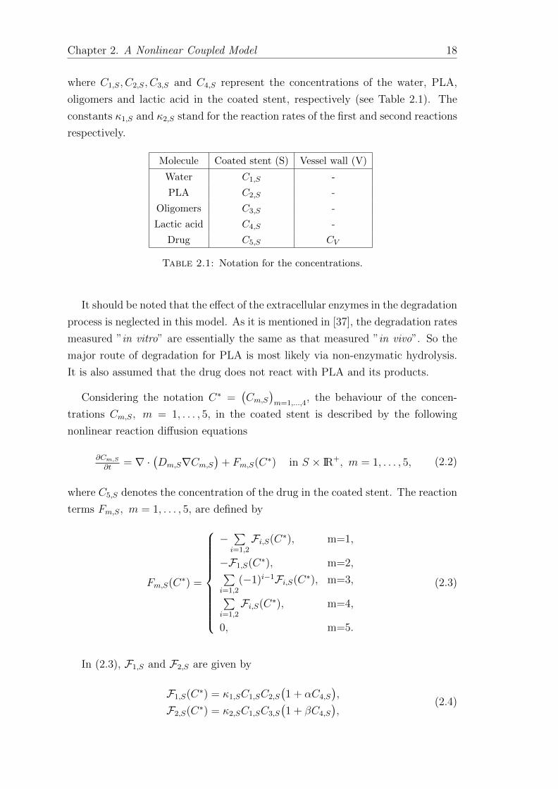
where C1,S, C2,S, C3,S and C4,S represent the concentrations of the water, PLA,
oligomers and lactic acid in the coated stent, respectively (see Table 2.1). The
constants κ1,S and κ2,S stand for the reaction rates of the first and second reactions
respectively.
Molecule Coated stent (S) Vessel wall (V)
Water C1,S -
PLA C2,S -
Oligomers C3,S -
Lactic acid C4,S -
Drug C5,S CV
Table 2.1: Notation for the concentrations.
It should be noted that the effect of the extracellular enzymes in the degradation
process is neglected in this model. As it is mentioned in [37], the degradation rates
measured ”in vitro” are essentially the same as that measured ”in vivo”. So the
major route of degradation for PLA is most likely via non-enzymatic hydrolysis.
It is also assumed that the drug does not react with PLA and its products.
Considering the notation C∗ =(Cm,S
)m=1,...,4
, the behaviour of the concen-
trations Cm,S, m = 1, . . . , 5, in the coated stent is described by the following
nonlinear reaction diffusion equations
∂Cm,S∂t
= ∇ ·(Dm,S∇Cm,S
)+ Fm,S(C∗) in S × IR+, m = 1, . . . , 5, (2.2)
where C5,S denotes the concentration of the drug in the coated stent. The reaction
terms Fm,S, m = 1, . . . , 5, are defined by
Fm,S(C∗) =
−∑i=1,2
Fi,S(C∗), m=1,
−F1,S(C∗), m=2,∑i=1,2
(−1)i−1Fi,S(C∗), m=3,∑i=1,2
Fi,S(C∗), m=4,
0, m=5.
(2.3)
In (2.3), F1,S and F2,S are given by
F1,S(C∗) = κ1,SC1,SC2,S
(1 + αC4,S
),
F2,S(C∗) = κ2,SC1,SC3,S
(1 + βC4,S
),
(2.4)

Chapter 2. A Nonlinear Coupled Model 19
where α and β are positive dimensional constants. The negative signs in (2.3)
indicate the consumption of molecules while the positive signs indicate the pro-
duction of molecules. For instance, the reaction term for the water is represented
by
−κ1,SC1,SC2,S − κ1,SαC1,SC2,SC4,S − κ2,SC1,SC3,S − κ2,SβC1,SC3,SC4,S. (2.5)
The reaction term (2.5) indicates that PLA degrades into oligomers and lactic
acid and also oligomers hydrolyze producing lactic acid. The negative signs in
(2.5) indicate that the water is consumed during the time (see (2.1)). The other
reaction terms in (2.3) have similar interpretations.
The diffusivities of the water, oligomers, lactic acid and drug will evolve with
time. This variation occurs due to the progressive degradation of the polymer
as well as due to the swelling of the polymer. It is therefore assumed that the
diffusion coefficients increase exponentially with the extent of the hydrolysis of
PLA ([34, 38]). The diffusivity coefficients in the coated stent are represented by
Dm,S = D0m,Se
αm,SC0
2,S−C2,S
C02,S in S × IR+, m = 1, . . . , 5, (2.6)
where D0m,S, m = 1, . . . , 5, are the diffusivity of the respective species in the
unhydrolyzed PLA and C02,S is the unhydrolyzed polymer concentration at the
initial time.
For the arterial wall, the following simplified model
∂CV∂t
= ∇ ·(DV∇CV
)in V × IR+, (2.7)
with constant diffusion coefficient, DV is assumed where CV stands for the con-
centration of drug in the arterial wall.
Since the degradation starts at t = 0, we assume that there are no initial
oligomers and lactic acid in the coating. The drug and PLA are distributed uni-
formly. In the coated stent and the arterial wall, the initial conditions are defined
by C1,S(0) = C3,S(0) = C4,S(0) = 0, C2,S(0) = C5,S(0) = 1 in S,
CV (0) = 0 in V.(2.8)
Here and in what follows we denote by v(t) a function that depends on x, y and t,
that is for each t, v(t) : Ω −→ IR, where Ω represents S or V .

Chapter 2. A Nonlinear Coupled Model 20
We also assume that the boundary Γ1, interface between the coating and the
stent structure, is impermeable to the molecules present in the coated stent which
means that no mass flux crosses it, that is
Dm,S∇Cm,S · ηS = 0 on Γ1 × IR+, m = 1, . . . , 5, (2.9)
where ηS is the unit exterior normal to Γ1.
We assume that the blood flow in the arterial lumen does not significantly in-
fluence the drug release in the arterial wall. In Γ2 and Γ3, the boundary conditions
are defined byD1,S∇C1,S · ηS = γ1,S(1− C1,S) on (Γ2 ∪ Γ3)× IR+,
Dm,S∇Cm,S · ηS = −γm,SCm,S on (Γ2 ∪ Γ3)× IR+, m = 2, . . . , 5,(2.10)
where γm,S, m = 1, . . . , 5, represent transference coefficients.
We consider now the issue of finding effective coupling conditions across the
interface Γ4 which separates the coated stent and the arterial wall. The obvi-
ous condition to assign, at a permeable interface, is the continuity of the drug
concentration and the other condition is the continuity of its flux, that isD5,S∇C5,S · ηS = −DV∇CV · ηV on Γ4 × IR+,
C5,S = CV on Γ4 × IR+,(2.11)
where ηS = −ηV on Γ4. It is also assumed that Γ4 is impermeable to PLA, lactic
acid and oligomers.
In what concerns the interface boundary between intima and media, a Robin
boundary condition of type
DV∇CV · ηV = −γvCV on Γ7 × IR+, (2.12)
is considered for the drug. The boundary condition (2.12) means that the drug
can pass from intima to media.
A homogeneous Neumann boundary condition
DV∇CV · ηV = 0 on (Γ8 ∪ Γ9)× IR+, (2.13)
is assumed for the virtual boundaries Γ8 ∪ Γ9.

Chapter 2. A Nonlinear Coupled Model 21
The flux of drug from the arterial wall to the blood is given by
DV∇CV · ηV = −γbCV on (Γ5 ∪ Γ6)× IR+, (2.14)
where γb is such that the endothelium layer offers a small resistance to the drug
transport.
Summarizing, the boundary and interface conditions are defined by
Dm,S∇Cm,S · ηS = 0 on Γ1 × IR+, m = 1, . . . , 5,
D1,S∇C1,S · ηS = γ1,S(1− C1,S) on (Γ2 ∪ Γ3)× IR+,
Dm,S∇Cm,S · ηS = −γm,SCm,S on (Γ2 ∪ Γ3)× IR+, m = 2, . . . , 5,
Dm,S∇Cm,S · ηS = 0 on Γ4 × IR+, m = 1, . . . , 4,
C5,S = CV on Γ4 × IR+,
D5,S∇C5,S · ηS = −DV∇CV · ηV on Γ4 × IR+,
DV∇CV · ηV = −γbCV on (Γ5 ∪ Γ6)× IR+,
DV∇CV · ηV = −γvCV on Γ7 × IR+,
DV∇CV · ηV = 0 on (Γ8 ∪ Γ9)× IR+.
(2.15)
2.2 Qualitative behavior of the total mass
In what follows we analyze the time behavior of the total mass
M(t) =
5∑m=1
∫S
Cm,S(t)dS +
∫V
CV (t)dV, (2.16)
where the notations have been presented in Table 2.1.
Replacing (2.2) and (2.7) in
M′(t) =5∑
m=1
∫S
∂Cm,S∂t
(t)dS +
∫V
∂CV∂t
(t)dV, (2.17)
we obtain
M′(t) =
5∑m=1
∫S
(∇ ·(Dm,S(t)∇Cm,S(t)
)+ Fm,S(C∗(t))
)dS +
∫V
∇ ·(DV∇CV (t)
)dV.(2.18)
Using Gauss’s theorem ([11]), taking into account the boundary conditions
(2.9), (2.10), (2.12), (2.13) and (2.14), and reaction terms (2.3) and (2.4), we

Chapter 2. A Nonlinear Coupled Model 22
deduce
M′(t) = γ1,S
∫Γ2∪Γ3
(1− C1,S(t))ds−4∑
m=2
γm,S
∫Γ2∪Γ3
Cm,S(t)ds− γb∫
Γ5∪Γ6
CV (t)ds
+
∫Γ4
D5,S(t)∇C5,S(t) · ηSds+
∫Γ4
DV∇CV (t) · ηV ds− γ5,S
∫Γ2∪Γ3
C5,S(t)ds
−γv∫
Γ7
CV (t)ds−∫S
κ2,SC1,S(t)C3,S(t)(1 + βC4,S(t)
)dS.
(2.19)
Replacing the coupling conditions (2.11) in (2.19), we have
M′(t) = −∆MΓ(t)−∆MH(t) + γ1,S
∣∣∣∣Γ2 ∪ Γ3
∣∣∣∣, (2.20)
where
∆MΓ(t) =5∑
m=1
γm,S
∫Γ2∪Γ3
Cm,S(t)ds+ γv
∫Γ7
CV (t)ds+ γb
∫Γ5∪Γ6
CV (t)ds, (2.21)
and the mass of hydrolyzed oligomers is given by
∆MH(t) =
∫S
κ2,SC1,S(t)C3,S(t)(1 + βC4,S(t)
)dS, (2.22)
and
∣∣∣∣Γ2 ∪ Γ3
∣∣∣∣ represents the length of the boundary segment Γ2 ∪ Γ3.
We note that ∆MΓ(t) represents the mass of molecules that enters, per unit
time, in the lumen; ∆MH(t) stands for the mass of lactic acid produced by unit
time, and resulting from the hydrolysis of oligomers.
Finally, by integrating in time we deduce
M(t) =M(0) + γ1,S
∣∣∣∣Γ2 ∪ Γ3
∣∣∣∣t−∫ t
0
∆MH(µ) dµ−∫ t
0
∆MΓ(µ) dµ. (2.23)
The equality (2.23) means that the total mass of the system at time t is given
by the difference between the initial mass added to the mass of water that enters
in the system until time t, and the mass of hydrolyzed oligomers until time t, the
mass of the components that are on the boundary until time t.

Chapter 2. A Nonlinear Coupled Model 23
2.3 Weak formulation of the coupled problems
In this section, we introduce a variational problem associated with the initial
boundary value problem (IBVP) (2.2)− (2.7) and (2.15).
Let Ω be a bounded domain in IR2 with boundary ∂Ω. We denote by L2(Ω)
and H1(Ω) the usual Sobolev spaces endowed with the usual inner products (., .)
and (., .)1 and norms ‖.‖L2(Ω) and ‖.‖H1(Ω) respectively (see [3]).
The space of functions v : (0, T ) −→ H1(Ω) such that∫ T
0
∥∥v(t)∥∥2
H1(Ω)dt <∞, (2.24)
will be denoted by L2(0, T ;H1(Ω)). By L∞(0, T ;L∞(Ω)) we represent the space
of functions v : (0, T ) −→ L∞(Ω) such that
ess sup(0,T )
∥∥v(t)∥∥L∞(Ω)
<∞. (2.25)
Let ΩS,V = S ∪ V ∪ Γ4 and let C, γ and D be defined by
C =
C5,S in S × (0, T ],
CV in V × (0, T ],(2.26)
γ =
γ5,S on Γ2 ∪ Γ3,
γb on Γ5 ∪ Γ6,
γv on Γ7,
(2.27)
and
D =
D05,Se
α5,S
C02,S−C2,S
C02,S in S × (0, T ],
DV in V × (0, T ].(2.28)
We remark that C5,S = CV on S ∩ V .
The weak solution of the IBVP (2.2)−(2.7) and (2.15) is defined by the following
variational problem:

Chapter 2. A Nonlinear Coupled Model 24
VP1: Find (C∗, C) ∈(L2(0, T ;H1(S))
)4
× L2(0, T ;H1(ΩS,V )) such that(∂C∗
∂t, ∂C∂t
)∈(L2(0, T ;L2(S))
)4
× L2(0, T ;L2(ΩS,V )) and
4∑m=1
(∂Cm,S∂t (t), vm
)S
+
(∂C∂t (t), w
)ΩS,V
= −4∑
m=1
(Dm,S∇Cm,S(t),∇vm
)S
−(D∇C(t),∇w
)ΩS,V
+
4∑m=1
(Fm,S(C∗(t)), vm
)S
+γ1,S
(1− C1,S(t), v1
)Γ2∪Γ3
−4∑
m=2
γm,S
(Cm,S(t), vm
)Γ2∪Γ3
−(γC(t), w
)Γ
,
a.e. in (0, T ), for all vm ∈ H1(S), m = 1, . . . , 4, and w ∈ H1(ΩS,V ),
C∗(0) = (0, 1, 0, 0),
C(0) = χS ,
(2.29)
where χS =
1 in S,
0 in V,and Γ = Γ2 ∪ Γ3 ∪ Γ5 ∪ Γ6 ∪ Γ7.
In what follows we study the behavior of the solution of the variational problem
VP1 assuming that the diffusion coefficients Dm,S, m = 1, . . . , 5, are constants.
We represent by L∞(L∞) the space L∞(0, T ;L∞(Ω)). Let the energy functional
E∇(t) be defined by
E∇(t) =
4∑m=1
(∥∥∥∥Cm,S(t)
∥∥∥∥2
L2(S)
+ 2
∫ t
0
∥∥∥∥√Dm,S∇Cm,S(s)
∥∥∥∥2
L2(S)
ds
)+
∥∥∥∥C(t)
∥∥∥∥2
L2(ΩS,V )
+2
∫ t
0
∥∥∥∥√D∇C(s)
∥∥∥∥2
L2(ΩS,V )
ds, t ∈ [0, T ],
(2.30)
where E∇(0) is the initial energy that depends only on PLA and drug.
Theorem 2.3.1. If (C∗, C) is a solution of the variational problem VP1 such that
Cm,S(t) ∈ H2(S), m = 1, . . . , 4, then there exists a positive constant K depending
on ‖C∗‖L∞(L∞) = maxm=1,...,4
∥∥Cm,S∥∥L∞(L∞), such that the following holds
E∇(t) ≤ e2KtE∇(0) +γ1,S
2K
∣∣∣∣Γ2 ∪ Γ3
∣∣∣∣(e2Kt − 1), t ∈ [0, T ], (2.31)
where
∣∣∣∣Γ2 ∪ Γ3
∣∣∣∣ is the length of the boundary layer Γ2 ∪ Γ3.

Chapter 2. A Nonlinear Coupled Model 25
Proof. We take in (2.29), vm = Cm,S(t), m = 1, . . . , 4, and w = C(t). It is not
difficult to check that(dCm,Sdt
(t), Cm,S(t)
)S
=
∫S
dCm,Sdt
(t)Cm,S(t)dS
=1
2
d
dt
∫S
C2m,S(t)dS =
1
2
d
dt
∥∥∥∥Cm,S(t)
∥∥∥∥2
L2(S)
,(2.32)
for m = 1, . . . , 4.
With the same approach we have(dC
dt(t), C(t)
)ΩS,V
=1
2
d
dt
∥∥∥∥C(t)
∥∥∥∥2
L2(ΩS,V )
. (2.33)
We also have(Dm,S∇Cm,S(t),∇Cm,S(t)
)S
=d
dt
∫ t
0
∥∥∥∥√Dm,S∇Cm,S(s)
∥∥∥∥2
L2(S)
ds, m = 1, . . . , 4,(D∇C(t),∇C(t)
)ΩS,V
=d
dt
∫ t
0
∥∥∥∥√D∇C(s)
∥∥∥∥2
L2(ΩS,V )
ds.
(2.34)
Summing up (2.32), (2.33) and (2.34) and taking into account (2.30), we obtain
1
2
d
dtE∇(t) =
4∑m=1
(Fm,S(C∗(t)), Cm,S(t)
)S
+ γ1,S
(1− C1,S(t), C1,S(t)
)Γ2∪Γ3
−4∑
m=2
γm,S
∥∥∥∥Cm,S(t)
∥∥∥∥2
L2(Γ2∪Γ3)
− γ∥∥∥∥C(t)
∥∥∥∥2
L2(Γ)
.
(2.35)
By Cauchy inequality ([11]) with ε = 12, we have(
1− C1,S(t), C1,S(t)
)Γ2∪Γ3
=
∫Γ2∪Γ3
(C1,S(t)− C2
1,S(t)
)ds ≤ 1
4
∣∣∣∣Γ2 ∪ Γ3
∣∣∣∣ (2.36)
Consequently the inequality (2.35) leads to
1
2
d
dtE∇(t) ≤
4∑m=1
(Fm,S(C∗(t)), Cm,S(t)
)S
+γ1,S
4
∣∣∣∣Γ2 ∪ Γ3
∣∣∣∣. (2.37)
As H2(S) is embedded in the space of continuous bounded functions in S
([3]), it can be shown that there exists a positive constant K that depends on
Chapter 2. A Nonlinear Coupled Model 26
∥∥C∗∥∥L∞(L∞)= max
m=1,...,4
∥∥Cm,S∥∥L∞(L∞), such that
4∑m=1
(Fm,S(C∗(t)), Cm,S(t)
)S
≤ K4∑
m=1
∥∥∥∥Cm,S(t)
∥∥∥∥2
L2(S)
. (2.38)
Inequality (2.37) leads to the differential inequality
d
dtE∇(t) ≤ 2KE∇(t) +
γ1,S
2
∣∣∣∣Γ2 ∪ Γ3
∣∣∣∣. (2.39)
By multiplying both sides of (2.39) by e−Kt and integrating over time, we finally
deduce (2.31).
2.4 Stability analysis
We consider in what follows two solutions C(t) = (C∗(t), C(t)) and C(t) =
(C∗(t), C(t)) with different initial conditions C(0) and C(0), respectively. We recall
that C∗(t) =(Cm,S(t)
)m=1,...,4
, where Cm,S, m = 1, . . . , 4, are defined in Table 2.1.
To study the stability of the IBVP (2.2)-(2.7) and (2.15), we should verify that∥∥∥∥C∗(t)− C∗(t)∥∥∥∥2
L2(S)
+
∥∥∥∥C(t)− C(t)
∥∥∥∥2
L2(ΩS,V )
≤ B(t)(∥∥∥∥C∗(0)− C∗(0)
∥∥∥∥2
L2(S)
+
∥∥∥∥C(0)− C(0)
∥∥∥∥2
L2(ΩS,V )
),
(2.40)
for t ∈ [0, T ], where
∥∥∥∥C∗(t)− C∗(t)∥∥∥∥L2(S)
=4∑
m=1
∥∥∥∥Cm,S(t)− Cm,S(t)
∥∥∥∥L2(S)
and B(t)
is bounded in time.
To establish the inequality (2.40) it is sufficient to assume that the reaction
terms have bounded partial derivatives. As reaction terms (2.3) are nonlinear
functions without bounded partial derivatives, it is not possible in this case to
establish (2.40). To gain some insights on the stability behavior of the initial
value problem VP1, we study in what follows the stability of a linearization of
VP1 in the neighborhood of a solution C(t).
Chapter 2. A Nonlinear Coupled Model 27
We recall that C and D are defined by (2.26) and (2.28) respectively. Then the
system of equations (2.2) and (2.7) can be rewritten in the following formdCdt
(t) = F(C(t)), t > 0,
C(0) is given,(2.41)
with C(t) =(C∗(t), C(t)
)and F(C(t)) =
(Fm(C(t))
)m=1,...,5
is represented by
Fm(C(t)) = ∇ ·
(Dm,S∇Cm,S(t)
)+ Fm,S(C∗(t)), m = 1, . . . , 4,
F5(C(t)) = ∇ ·(D∇C(t)
),
(2.42)
and Fm,S(C∗(t)), m = 1, . . . , 4, are defined by (2.3) and (2.4). We also assume
that conditions (2.15) hold.
The linearization of the initial value problem (2.41) in C(t) can be written in
the following form dCdt
(t) = LC(t) , t > 0,
C(0) is given,(2.43)
where LC(t) =
(LmC(t)
)m=1,...,5
is defined by
LmC(t) = ∇ ·
(Dm,S∇Cm,S(t)
)+ FJ,m(C(t))C(t), m = 1, . . . , 4,
L5C(t) = ∇ ·(D∇C(t)
),
(2.44)
C(t) = (C∗(t), C(t)), C∗(t) =
(Cm,S(t)
)m=1,...,4
and
FJ,m(C(t))C(t) =
−∑i=1,2
FJ,i(C(t))C(t), m=1,
−FJ,1(C(t))C(t), m=2,∑i=1,2
(−1)i−1FJ,i(C(t))C(t), m=3,∑i=1,2
FJ,i(C(t))C(t), m=4.
(2.45)

Chapter 2. A Nonlinear Coupled Model 28
In (2.45), FJ,i(C(t))C(t), i = 1, 2, represent Frechet derivatives given byFJ,1(C(t))C(t) = κ1,SC2,S(t)(1 + αC4,S(t))C1,S(t) + κ1,SC1,S(t)(1 + αC4,S(t))C2,S(t)
+κ1,SαC1,S(t)C2,S(t)C4,S(t),
FJ,2(C(t))C(t) = κ2,SC3,S(t)(1 + βC4,S(t))C1,S(t) + κ2,SC1,S(t)(1 + βC4,S(t))C3,S(t)
+κ2,SβC1,S(t)C3,S(t)C4,S(t).
(2.46)
Let C and ˜C be solutions of the variational problem associated with the IBVP
defined by (2.43) and conditions (2.15), with initial conditions C(0) and ˜C(0) in
which C(t), ˜C(t) ∈(H2(S)
)4
.
We establish in what follows an upper bound for the functional EW(t) defined
by
EW(t) =
4∑m=1
∥∥∥∥Wm,S(t)
∥∥∥∥2
L2(S)
+
∥∥∥∥W (t)
∥∥∥∥2
L2(ΩS,V )
, t ∈ [0, T ], (2.47)
where Wm,S = Cm,S − ˜Cm,S, m = 1, . . . , 4, and
W =
C5,S − ˜C5,S in S,
CV − ˜CV in V.(2.48)
It can be shown that
1
2
d
dtEW(t) ≤ −
4∑m=1
∥∥∥∥√Dm,S∇Wm,S(t)
∥∥∥∥2
L2(S)
−∥∥∥∥√D∇W (t)
∥∥∥∥2
L2(ΩS,V )
+4∑
m=1
(FJ,m(C(t))Wm,S(t),Wm,S(t)
)S.
(2.49)
Consequently, there exists a positive constant K′ depending on∥∥C∗∥∥L∞(L∞)
such that
d
dtEW(t) ≤ 2K′EW(t), t > 0. (2.50)
This inequality leads to
EW(t) ≤ e2K′tEW(0), (2.51)

Chapter 2. A Nonlinear Coupled Model 29
which allow us to conclude the stability of the linearization of VP1 for short
periods of time.
2.5 Finite dimensional approximation
To define a finite dimensional approximation for the solution of VP1, we fix
h > 0 and introduce in ΩS,V an admissible triangulation Th such that the corre-
spondent admissible triangulations induced in S and V, respectively ThS and ThV ,
are compatible on Γ4 (see Figure 2.3).
Let C∗h =
(Cm,S,h
)m=1,...,4
, stand for an approximation of C∗ and
Ch =
C5,S,h in S × (0, T ],
CV,h in V × (0, T ],(2.52)
where C5,S,h = CV,h on Γ4, represent an approximation of C.
To compute the semi-discrete Ritz-Galerkin approximation Ch = (C∗h, Ch) for
the weak solution C = (C∗, C) defined by VP1, we introduce in what follows the
finite dimensional spaces
PrΩ =
u ∈ C0(Ω) : u
∣∣∆
= Pr, ∆ ∈ ThΩ
, (2.53)
where Ω = S,ΩS,V and Pr denotes a polynomial in the space variables with degree
at most r and C0(Ω) denotes the space of continuous functions in Ω.
The Ritz-Galerkin approximation Ch is then computed by solving the following
variational problem:
FEVP1: Find (C∗h(t), Ch(t)) ∈(PrS)4 × PrΩS,V such that
4∑m=1
(∂Cm,S,h
∂t (t), vm,h
)S
+
(∂Ch∂t (t), wh
)ΩS,V
= −4∑
m=1
(Dm,S,h∇Cm,S,h(t),∇vm,h
)S
−(Dh∇Ch(t),∇wh
)ΩS,V
+
4∑m=1
(Fm,S(C∗h(t)), vm,h
)S
+γ1,S
(1− C1,S,h(t), v1,h
)Γ2∪Γ3
−(γCh(t), wh
)Γ
−4∑
m=2
γm,S
(Cm,S,h(t), vm,h
)Γ2∪Γ3
in (0, T ], for all vm,h ∈ PrS , m = 1, . . . , 4, and wh ∈ PrΩS,V ,C∗h(0) = (0, 1, 0, 0),
Ch(0) = χS .
(2.54)

Chapter 2. A Nonlinear Coupled Model 30
In (2.54), Dm,S,h = D0m,Se
αm,SC0
2,S−C2,S,h
C02,S in S × (0, T ], m = 1, . . . , 4, and
Dh =
D05,Se
α5,S
C02,S−C2,S,h
C02,S in S × (0, T ],
DV in V × (0, T ].
Following the proof of Theorem 2.3.1, it can be shown that a semi-discrete
version of E∇(t), defined by the Ritz-Galerkin approximation Ch, satisfies an in-
equality analogous to (2.31). Moreover, for the linearization of FEVP1 around
Ch, it can be shown an inequality analogous to (2.51).
2.6 Full discrete IMEX problem
We introduce in [0, T ] a uniform grid
tn;n = 0, . . . , N
with t0 = 0, tN = T ,
tn − tn−1 = ∆t. By D−t we denote the backward finite difference operator with
respect to time variable t. The weak solution of the problem in the full discrete
case is the solution of the following finite dimensional variational formulation:
Find (C∗,n+1h , Cn+1
h ) ∈(PrS)4 × PrΩS,V such that
4∑m=1
(D−t(C
∗,n+1h ), vm,h
)S
+
(D−t(C
n+1h ), wh
)ΩS,V
= −4∑
m=1
(Dnm,S,h∇C
n+1m,S,h,∇vm,h
)S
−(Dnh∇C
n+1h ,∇wh
)ΩS,V
+
4∑m=1
(Fm,S(Cn
∗
h ), vm,h
)S
+γ1,S
(1− Cn+1
1,S,h, v1,h
)Γ2∪Γ3
−(γCn+1
h , wh
)Γ
−4∑
m=2
γm,S
(Cn+1m,S,h, vm,h
)Γ2∪Γ3
,
for all vm,h ∈ PrS , m = 1, . . . , 4, and wh ∈ PrΩS,V ,C∗,0h = (0, 1, 0, 0),
C0h = χS ,
(2.55)
for n = 0, . . . , N , where
Fm,S(Cn∗
h ) =
−κ1,SCn+11,S,hC
n2,S,h
(1 + αCn4,S,h
)− κ2,SC
n+11,S,hC
n3,S,h
(1 + βCn4,S,h
), m=1,
−κ1,SCn+11,S,hC
n+12,S,h
(1 + αCn4,S,h
), m=2,
κ1,SCn+11,S,hC
n+12,S,h
(1 + αCn4,S,h
)− κ2,SC
n+11,S,hC
n+13,S,h
(1 + βCn4,S,h
), m=3,
κ1,SCn+11,S,hC
n+12,S,h
(1 + αCn+1
4,S,h
)+ κ2,SC
n+11,S,hC
n+13,S,h
(1 + βCn+1
4,S,h
), m=4,
0, m=5,
(2.56)
are reaction functions of the problem in the implicit-explicit (IMEX) form.

Chapter 2. A Nonlinear Coupled Model 31
2.7 Numerical experiments
In this section we illustrate the behaviour of the numerical solution defined by
(2.55) as well as the influence of the parameters of the model in the release rate. All
experiments have been done with open source partial differential equation solver
freeFEM++ ([19]) with 10096 elements (5224 vertices) for ΩS,V and 3250 elements
(1751 vertices) for the stent S, and using IMEX backward integrator with time
step size ∆t = 10−3.
Figure 2.3: Triangulation in the stent and in the arterial wall.
The following parameters have been used for the modeling of the drug release
from the drug eluting stent into the arterial wall:
γm,S = 105 cm/s, m = 1, . . . , 5, γv = 105 cm/s, γb = 1010 cm/s, αm,S = 9, m =
1, . . . , 4, α5,S = 0.9, κ1,S = 10−6 cm2/g.s, κ2,S = 10−8 cm2/g.s, α = 1 s/cm2,
β = 10 s/cm2, D01,S = 5×10⁻⁷ cm2/s, D0
2,S = 10−15 cm2/s, D03,S = 5×10⁻¹² cm2/s,
D04,S = 3× 10⁻¹² cm2/s, D0
5,S = 2× 10⁻⁸ cm2/s, DV = 5× 10⁻⁸ cm2/s.
Several choices of finite element spaces can be made, but we consider here the
piecewise linear finite element space P1 ([36]).
In Figures 2.4-2.6, we plot the drug distribution in the stent and in the arterial
wall after 1 day, 7 and 14 days. When the drug reaches Γ4 (see Figure 2.1), it
crosses this interface boundary to the arterial wall as mathematically described by
(2.11). When the drug reaches the boundary Γ7, it enters the media as described
by Robin boundary condition (2.12).

Chapter 2. A Nonlinear Coupled Model 32
Figure 2.4: Drug distribution in the coating and the arterial wall after 1 day.
Figure 2.5: Drug distribution in the coating and the arterial wall after 7 days.
Figure 2.6: Drug distribution in the coating and the arterial wall after 14days.

Chapter 2. A Nonlinear Coupled Model 33
In Figures 2.7-2.9, we exhibit the penetration of the water into the coated stent.
We observe that the water penetrates into the PLA until it reaches a steady state
level.
Figure 2.7: Concentration of water in the coating after 1 day.
Figure 2.8: Concentration of water in the coating after 7 days.
Figure 2.9: Concentration of water in the coating after 14 days.

Chapter 2. A Nonlinear Coupled Model 34
Figure 2.10: Concentration of PLA in the coating after 1 day.
Figure 2.11: Concentration of PLA in the coating after 7 days.
Figure 2.12: Concentration of PLA in the coating after 14 days.
Chapter 2. A Nonlinear Coupled Model 35
In Figures 2.10-2.12, the degradation of PLA into smaller molecules which are
released into the lumen is shown. It is assumed that the penetration of the PLA
and also its products, oligomers and lactic acid, into the arterial wall are negligible.
The evolution of PLA concentration is compatible with erosion during degradation.
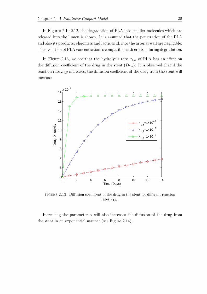
In Figure 2.13, we see that the hydrolysis rate κ1,S of PLA has an effect on
the diffusion coefficient of the drug in the stent (D5,S). It is observed that if the
reaction rate κ1,S increases, the diffusion coefficient of the drug from the stent will
increase.
0 2 4 6 8 10 12 145
6
7
8
9
10
11
12
13
14x 10
−8
Time (Days)
Dru
g D
iffus
ivity
κ1,S
=1×10⁻⁷
κ1,S
=1×10⁻⁶
κ1,S
=1×10⁻⁵
Figure 2.13: Diffusion coefficient of the drug in the stent for different reactionrates κ1,S .
Increasing the parameter α will also increases the diffusion of the drug from
the stent in an exponential manner (see Figure 2.14).

Chapter 2. A Nonlinear Coupled Model 36
0 2 4 6 8 10 12 145
6
7
8
9
10
11
12
13
14x 10
−8
Time (Days)
Dru
g D
iffus
ivity
κ1,S
=1×10⁻⁶, α=1
κ1,S
=1×10⁻⁶, α=5
Figure 2.14: Diffusion coefficient of the drug in the stent for different valuesof α.
We define the mass of species in the coated stent and the mass of drug in the
arterial wall by
Mm,S,h(tn) =
∫S
Cm,S,h(tn)dS, m = 1, . . . , 5, MV,h(tn) =
∫V
CV,h(tn)dV, (2.57)
respectively, where Mm,S,h(tn) and MV,h(tn) are the numerical approximations for
masses at time level tn.
In Figures 2.15-2.18, we exhibit the mass of drug as well as the mass of the
water, PLA and lactic acid in the coated stent during the first 2 weeks after stent
implantation using different diffusion coefficients of drug in the stent.

Chapter 2. A Nonlinear Coupled Model 37
0 2 4 6 8 10 12 140
0.01
0.02
0.03
0.04
0.05
0.06
0.07
0.08
0.09
0.1
Time (days)
Mas
s
Water, D01,S
=5×10⁻⁸
Water, D01,S
=5×10⁻⁹
Figure 2.15: Mass of water in the stent for different values of D01,S .
0 2 4 6 8 10 12 140.82
0.84
0.86
0.88
0.9
0.92
0.94
0.96
0.98
1
Time (Days)
Mas
s
Drug in the stent, D01,S
=5×10⁻⁸
Drug in the stent, D01,S
=5×10⁻⁹
Figure 2.16: Mass of drug in the stent for different values of D01,S .

Chapter 2. A Nonlinear Coupled Model 38
0 2 4 6 8 10 12 140
0.02
0.04
0.06
0.08
0.1
0.12
0.14
0.16
Time (days)
Mas
s
Lactic acid, D01,S
=5×10⁻⁸
Lactic acid, D01,S
=5×10⁻⁹
Figure 2.17: Mass of lactic acid in the stent for different values of D01,S .
0 2 4 6 8 10 12 140.86
0.88
0.9
0.92
0.94
0.96
0.98
1
Time (Days)
Mas
s
PLA, D01,S
=5×10⁻⁸
PLA, D01,S
=5×10⁻⁹
Figure 2.18: Mass of PLA in the stent for different values of D01,S .
In Figures 2.15-2.18, we observe that small diffusion coefficients will decrease
the accumulation of drug and PLA degradation in the stent. It will also decrease
the mass of water and lactic acid in the stent.
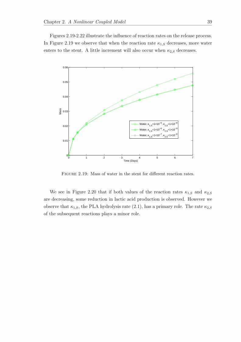
Chapter 2. A Nonlinear Coupled Model 39
Figures 2.19-2.22 illustrate the influence of reaction rates on the release process.
In Figure 2.19 we observe that when the reaction rate κ1,S decreases, more water
enters to the stent. A little increment will also occur when κ2,S decreases.
0 1 2 3 4 5 6 70
0.01
0.02
0.03
0.04
0.05
0.06
Time (Days)
Mas
s
Water, κ1,S
=1×10⁻⁶, κ2,S
=1×10⁻⁸
Water, κ1,S
=1×10⁻⁶, κ2,S
=1×10⁻⁹
Water, κ1,S
=1×10⁻⁷, κ2,S
=1×10⁻⁸
Figure 2.19: Mass of water in the stent for different reaction rates.
We see in Figure 2.20 that if both values of the reaction rates κ1,S and κ2,S
are decreasing, some reduction in lactic acid production is observed. However we
observe that κ1,S, the PLA hydrolysis rate (2.1), has a primary role. The rate κ2,S
of the subsequent reactions plays a minor role.

Chapter 2. A Nonlinear Coupled Model 40
0 1 2 3 4 5 6 70
0.005
0.01
0.015
0.02
0.025
0.03
0.035
0.04
0.045
0.05
Time (Days)
Mas
s
Lactic acid, κ1,S
=1×10⁻⁶, κ2,S
=1×10⁻⁸
Lactic acid, κ1,S
=1×10⁻⁶, κ2,S
=1×10⁻⁹
Lactic acid, κ1,S
=1×10⁻⁷, κ2,S
=1×10⁻⁸
Figure 2.20: Mass of lactic acid in the stent for different reaction rates.
Figures 2.21 and 2.22 indicate that a decrement in κ1,S will decelerate the speed
of drug release and PLA degradation in the stent.
0 1 2 3 4 5 6 70.88
0.9
0.92
0.94
0.96
0.98
1
Time (Days)
Mas
s
Drug, κ1,S
=1×10⁻⁶, κ2,S
=1×10⁻⁸
Drug, κ1,S
=1×10⁻⁷, κ2,S
=1×10⁻⁸
Figure 2.21: Mass of drug in the stent for different reaction rates.

Chapter 2. A Nonlinear Coupled Model 41
0 1 2 3 4 5 6 70.95
0.955
0.96
0.965
0.97
0.975
0.98
0.985
0.99
0.995
1
Time (Days)
Mas
s
PLA, κ1,S
=1×10⁻⁶, κ2,S
=1×10⁻⁸
PLA, κ1,S
=1×10⁻⁷, κ2,S
=1×10⁻⁸
Figure 2.22: Mass of PLA in the stent for different reaction rates.
In this chapter we focused on the influence of polymer degradation parameters
on the drug release from a DES into an arterial wall. The numerical results
obtained are physically sound. The clarification of degradation mechanisms and
the quantification of that influence can provide useful guidelines to manufacturers.
The model proposed in this chapter simulates ”in vivo” drug release. However the
viscoelastic properties of the vessel walls were not taken into account. A detailed
description of their rheological properties will be introduced in Chapter 3.


Chapter 3
A Non-Fickian Coupled Model
In this chapter, we will address to a more complex coupled model than the
one introduced in Chapter 2. We evolve from the model introduced in Section
2.1, where the transport of drug in the stent coating and in the arterial wall
is dominated by diffusion, to a model where convective transport of the drug
is considered and the viscoelastic properties of the arterial wall are taken into
account.
Experiments like creep test ([16, 29, 41]) have clearly demonstrated that the
vascular tissue is viscoelastic. Thus when a constant force is exerted on an artery
over an extended period of time, it will first deform like an elastic body and then
continue to deform or flow for a finite period of time.
Arterial stiffness is considered as an excellent indicator of cardiovascular mor-
bidity and mortality in a large percentage of the population as referenced in [20].
Taking into consideration the arterial stiffness in the mathematical modeling of
drug release from the stent into the arterial wall can help to understand the phar-
macokinetic effects of the drug in atherosclerosis.
During the last years, a number of studies have proposed mathematical models
for coupled drug delivery in the cardiovascular tissues. We refer without being
exhaustive to [2, 5, 18, 25, 28, 34, 46] and also [35] as a review paper. Most
of these studies address the release of drug and its numerical behavior while the
viscoelasticity of the arterial wall is disregarded.
In this chapter, we propose a non-Fickian coupled model for predicting the
biodegradation of PLA, as a drug carrier in the coated stent, and the simultaneous
release of the drug from the stent coating into the arterial wall. The effect of
43

Chapter 3. A Non-Fickian Coupled Model 44
viscoelasticity of the arterial wall in the drug release is investigated using Maxwell-
Wiechert model ([6]) and Fung’s quasilinear viscoelastic model ([16]).
The chapter is organized as follows. Section 3.1 is devoted to the description
of the model and its initial, boundary and interface conditions. In Section 3.2, we
explain the mass behavior of molecules from the viewpoint of a phenomenological
approach. In Section 3.3, we present a variational formulation and establish an
energy estimate for the continuous model. The stability of a linearized problem
is also studied. Using an implicit-explicit finite element method, we establish a
semi-discrete variational form in Section 3.4 and a full discrete variational form
in Section 3.5. Numerical simulations as well as a sensitivity analysis of the vis-
coelastic parameters are discussed in Section 3.6.
3.1 Description of the model
Let us consider a two dimensional domain obtained as a section of a three
dimensional realistic geometry. Due to the symmetry of the geometry, we consider
only a part of the section. We introduce the two dimensional domain S ⊂ IR2
which represents the polymeric coating of the stent and V ⊂ IR2 which represents
the arterial wall. A schematic representation of the two dimensional domain used
in this model is shown in Figure 3.1.
Figure 3.1: DES inside of the arterial wall (left: http://www.ibmt.med.uni-rostock.de/nachwuchsgruppe.html).
In Figure 3.1, for the sake of simplicity we have assumed that the DES is com-
pletely embedded in the arterial wall. This is a reasonable assumption because

Chapter 3. A Non-Fickian Coupled Model 45
of the complex dynamics of tissue healing and regrowth which takes place imme-
diately after DES implantation in the arterial wall. The evolution of neo-intima
around the stent is considered negligible ([26, 46]).
In addition to assumptions 2 and 4 in Section 2.1, the following assumptions
are also taken into consideration in the mathematical model:
1. Viscoelastic properties of the polymeric part of the stent is considered neg-
ligible;
2. The arterial wall is considered as an homogeneous porous medium with the
main properties of media;
3. Permeability and viscosity of the stent and arterial wall are considered con-
stants.
Chemical reactions, convection and non-Fickian diffusion are three main phe-
nomena which explain the kinetics of the drug and the biodegradable polymer.
3.1.1 Chemical reactions
The chemical reactions responsible for the degradation of PLA into oligomers
and lactic acid in the stent coating were presented in Section 2.1. We introduce
now the degradation of oligomers into lactic acid that occurs in the arterial wall.
Let C1,V denotes the concentration of water in the arterial wall. The concen-
tration of oligomers in the arterial wall is denoted by C3,V . By C4,V we denote the
concentration of lactic acid in the arterial wall. Finally, by C5,V we represent the
concentration of drug in the arterial wall (see Table 3.1).
Molecule Coated stent (S) Vessel wall (V)
Water C1,S C1,V
PLA C2,S -
Oligomers C3,S C3,V
Lactic acid C4,S C4,V
Drug C5,S C5,V
Table 3.1: Notation for the concentrations.
Reactions for the degradation of PLA in the stent are defined by (2.1). The
only reaction in the arterial wall is the hydrolysis of the oligomers resulting in

Chapter 3. A Non-Fickian Coupled Model 46
lactic acid. This reaction is schematically represented by
C1,V + C3,V
κ1,V−−−→ C4,V , (3.1)
where κ1,V denotes the reaction rate of the hydrolysis of oligomers in the arterial
wall.
The evolution in time and space of each concentration depends on the type of
chemical reaction involved: production or consumption reaction. To simplify the
presentation of the reaction terms that affect the behavior of each concentration,
we introduce the notations:
CS =
(Cm,S
)m=1,...,5
, CV =
(Cm,V
)m=1,...,5,m 6=2
, and C =(CS, CV
). (3.2)
Let Fm,S(CS), m = 1, . . . , 5, be defined by (2.3) and (2.4). In the arterial wall
we define the following reaction terms
Fm,V (CV ) =
−F1,V (CV ), m=1,
−F1,V (CV ), m=3,
F1,V (CV ), m=4,
0, m=5,
(3.3)
where F1,V (CV ) is given by
F1,V (CV ) = κ1,VC1,VC3,V
(1 + γC4,V
). (3.4)
In (3.4) γ is a positive dimensional constant.
3.1.2 Convection
The transport of oligomers, lactic acid and drug in the coated stent and in the
arterial wall occurs by diffusion and convection. The same phenomena occur in
the transport of PLA in the coated stent. The convection is caused by a pressure
gradient in the fluid. Let uV and pV represent the velocity and the pressure of the
plasma in the arterial wall. We assume that the plasma is incompressible, which
mathematically implies that the divergence of its velocity is zero, ∇·uV = 0. The
behavior of the plasma is described by Darcy’s law.

Chapter 3. A Non-Fickian Coupled Model 47
To prescribe suitable boundary conditions in the arterial wall, we require that
uV · ηV = 0 on Γwall for symmetry, where ηV represents the exterior unit normal.
Moreover, we observe that the filtration of the plasma inside the arterial wall is
driven by a decreasing pressure gradient from the inner layer of the artery (Γlumen)
to the outer layer of the artery (Γadv). By consequence we require that pV = plumen
on Γlumen and pV = padv on Γadv. We notice that plumen is assumed to be uniform
and independent of space and time variables on Γlumen. The velocity and the
pressure in the arterial wall satisfy the following equations:
uV = − kVµV∇pV in V,
∇ · uV = 0 in V,
pV = plumen on Γlumen,
pV = padv on Γadv,
uV · ηV = 0 on Γwall.
(3.5)
We assume in what follows that the incompressible plasma can penetrate inside
the coated stent. Let uS and pS represent the velocity and the pressure of fluid in
the stent. As the metallic part of the stent is rigid we consider no flux of plasma
in Γstrut. So the velocity and the pressure in the coated stent are described byuS = − kS
µS∇pS in S,
∇ · uS = 0 in S,
uS · ηS = 0 on Γstrut,
(3.6)
where ηS represents the exterior unit normal.
Systems of equations (3.5) and (3.6) are completed with the matching conditionspS = pV on Γcoat,
uS · ηS = −uV · ηV on Γcoat.(3.7)
The boundaries Γlumen, Γadv, Γwall, Γstrut and Γcoat introduced in (3.5), (3.6)
and (3.7) are defined in Figure 3.1. In (3.5) and (3.6), kS and kV are permeability
coefficients which characterize the capacity of the stent and arterial wall to allow
the flow of small molecules across them. These coefficients depend on the proper-
ties of the medium and also on the concentrations of PLA, oligomers, lactic acid
and drug in the stent and oligomers, lactic acid and drug in the arterial wall. To
simplify the model, we assume that kj, j = S, V, are constants.

Chapter 3. A Non-Fickian Coupled Model 48
In (3.5) and (3.6), µj, j = S, V, are the viscosities of the fluid in the stent and
the arterial wall respectively, which represents the resistance of the fluid to gradual
deformation. These coefficients depend on the chemical compounds presented in
the stent and in the arterial wall. To simplify, we assume in what follows that the
viscosities µj, j = S, V, are also constants.
3.1.3 Viscoelastic effects
Viscoelasticity is the ability of a material to exhibit both solid-like and fluid-like
behavior. Viscoelastic models have been widely used to characterize mechanistic
properties of the vascular tissues due to their ability to tailor both the viscoelas-
tic relaxation function and the nonlinear elastic stress-strain relation. Numerous
viscoelastic models, derived under different experimental conditions, have been
proposed in the literature. We refer without being exhaustive to [6, 27, 29, 39, 40].
A constitutive equation typically determines the relationship between the stress
(internal force) that a material is subjected and the strain (deformation) response.
A reliable constitutive model for arterial walls is an essential prerequisite for study-
ing mechanical factors of atherosclerosis.
Analogical models are currently used to describe viscoelasticity. The simplest
linear viscoelastic models are attributed to Maxwell, Voigt, and Kelvin ([6]). The
Maxwell fluid model is represented by a dashpot in series with an elastic spring.
The Voigt solid model is represented by a dashpot in parallel with an elastic spring.
The Kelvin model, also called the standard linear solid combines a Maxwell element
in parallel with an elastic spring.
In what follows, we present a linear viscoelastic model (Maxwell-Wiechert model,
[6]). The multiple relaxation times used in this model are well adapted to predict
viscoelastic behavior in living tissues ([29]). We postpone for a later section for
some considerations on the use of a nonlinear viscoelastic model (Fung’s quasilin-
ear viscoelastic model, [16]).
In the Maxwell-Wiechert model (Figure 3.2), the relation between the stress
and the strain is given by the following convolution integral:
σV (t) = −(krεV (t) +
∫ t
0
K(t− s)∂εV∂s
(s)ds
), (3.8)
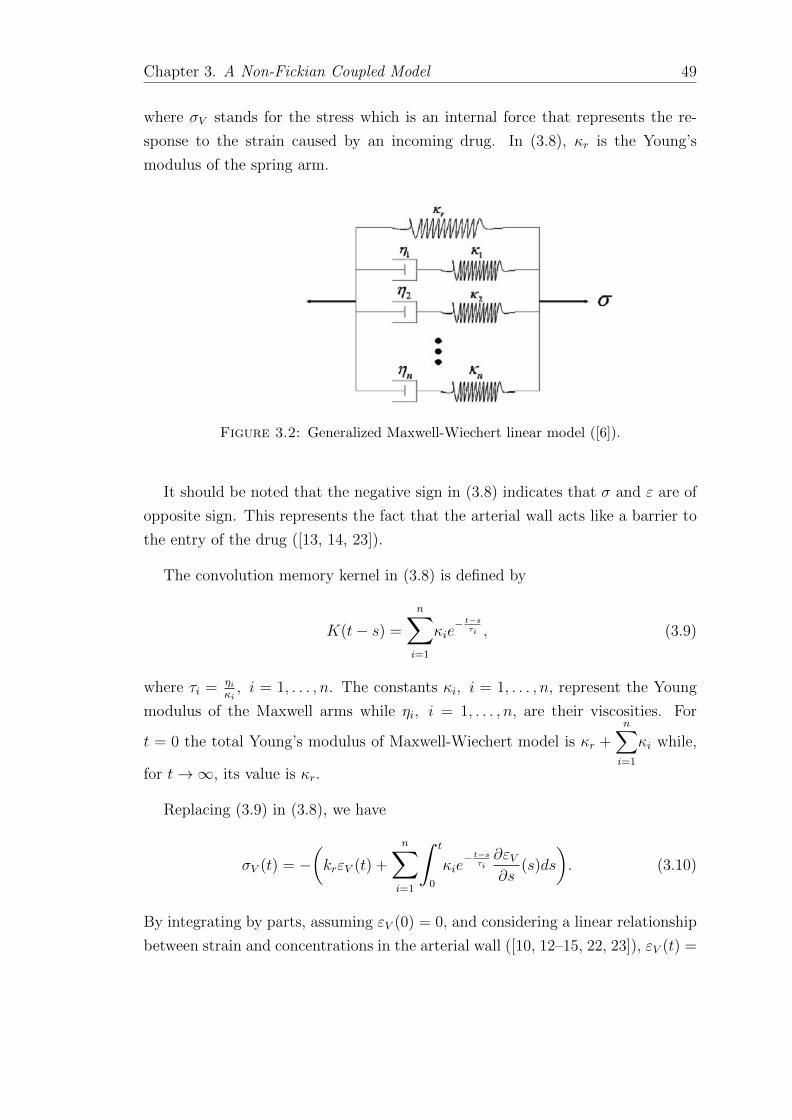
Chapter 3. A Non-Fickian Coupled Model 49
where σV stands for the stress which is an internal force that represents the re-
sponse to the strain caused by an incoming drug. In (3.8), κr is the Young’s
modulus of the spring arm.
Figure 3.2: Generalized Maxwell-Wiechert linear model ([6]).
It should be noted that the negative sign in (3.8) indicates that σ and ε are of
opposite sign. This represents the fact that the arterial wall acts like a barrier to
the entry of the drug ([13, 14, 23]).
The convolution memory kernel in (3.8) is defined by
K(t− s) =
n∑i=1
κie− t−s
τi , (3.9)
where τi = ηiκi, i = 1, . . . , n. The constants κi, i = 1, . . . , n, represent the Young
modulus of the Maxwell arms while ηi, i = 1, . . . , n, are their viscosities. For
t = 0 the total Young’s modulus of Maxwell-Wiechert model is κr +n∑i=1
κi while,
for t→∞, its value is κr.
Replacing (3.9) in (3.8), we have
σV (t) = −(krεV (t) +
n∑i=1
∫ t
0
κie− t−s
τi∂εV∂s
(s)ds
). (3.10)
By integrating by parts, assuming εV (0) = 0, and considering a linear relationship
between strain and concentrations in the arterial wall ([10, 12–15, 22, 23]), εV (t) =

Chapter 3. A Non-Fickian Coupled Model 50
αmCm,V (t), m = 1, . . . , 5, m 6= 2, we will finally have
σm,V (t) = −αm(
(κr +
n∑i=1
κi)Cm,V (t)−n∑i=1
κiτi
∫ t
0
e− t−s
τi Cm,V (s)ds
), (3.11)
for m = 1, . . . , 5, m 6= 2.
Particular attention will be devoted to the case n = 1, that is a mechanical
analog composed by an elastic arm and a Maxwell arm.
Figure 3.3: Maxwell-Wiechert model with n = 1 ([6]).
The following formulation
σm,V (t) = −αm(
(κr + κ1)Cm,V (t)− κ1
τ1
∫ t
0
e− t−s
τ1 Cm,V (s)ds
), (3.12)
for m = 1, . . . , 5, m 6= 2, is a particular case of (3.11) when n = 1.
3.1.4 A reaction-diffusion-convection problem
The reaction-convection-diffusion processes which take place in the stent are
described by the following system of equations
∂Cm,S∂t
= ∇ ·(Dm,S∇Cm,S − uSCm,S
)+ Fm,S(CS), (3.13)
in S × IR+, for m = 1, . . . , 5. The diffusion coefficients Dm,S, m = 1, . . . , 5, are
defined by (2.6), being of the variables summarized in Table 3.1.
The transport process that occurs in the arterial wall is due to convective
transport and non-Fickian diffusion driven by the stress. It is described by the

Chapter 3. A Non-Fickian Coupled Model 51
following set of equations
∂Cm,V∂t
= ∇ ·(Dm,V∇Cm,V − uV Cm,V
)+∇ ·
(Dσ∇σm,V
)+ Fm,V (CV ), (3.14)
in V × IR+, for m = 1, . . . , 5, m 6= 2.
We recall that the subscript m = 2 refers to PLA. As PLA has a large molecular
weight (MW ≥ 1.2 × 10⁵ g/mol) compared to the other species present in the
process, it will not cross the interface boundary Γcoat to enter the arterial wall. So
(3.14) is not applied for PLA.
It should be noted that the velocities uS and uV in (3.13) and (3.14) are
computed by solving the coupled problem (3.5)-(3.7). The reaction functions
Fm,j(Cj), j = S, V, in (3.13) and (3.14), are defined by (2.3), (2.4), (3.3) and
(3.4). In (3.14), the stress σm,V , m = 1, . . . , 5, m 6= 2, is given by (3.11) and Dσ
represents the ”weight” of the non-Fickian diffusion whose physical meaning can
be found in [13, 14].
In what follows, particular attention will be devoted to system (3.13) and
(3.14) when the viscoelastic behavior of the arterial wall is described by Maxwell-
Wiechert model with n = 1. The coupled problem (3.13) and (3.14) in this case
takes the form
∂Cm,S∂t = ∇ ·
(Dm,S∇Cm,S − uSCm,S
)+ Fm,S(CS) in S × IR+, m = 1, . . . , 5,
∂Cm,V∂t = ∇ ·
(Dm,V∇Cm,V − uV Cm,V
)+ Fm,V (CV )
+
∫ t
0e− t−s
τ1 ∇ ·(Dm,σ∇Cm,V (s)
)ds in V × IR+, m = 1, . . . , 5,m 6= 2,
(3.15)
where Dm,V = Dm,V −αm(κr +κ1)Dσ and Dm,σ = αmκ1
τ1Dσ for m = 1, . . . , 5, m 6=
2.
To ensure the positivity of the effective Fickian diffusion coefficient Dm,V , the
diffusion coefficients Dm,V , the Young modulus κr and κ1, the parameter αm and
the non-Fickian weight coefficient Dσ should satisfy the relation Dσ <Dm,V
αm(κr+κ1).
This assumption guarantees that Fickian diffusion dominates the viscoelastic op-
position, which is a physical condition for the effective penetration of drug in the
arterial wall.
For a sake of simplicity, we assume that the diffusion coefficients in the arterial
wall Dm,V , m = 1, . . . , 5, m 6= 2, are constants.
Chapter 3. A Non-Fickian Coupled Model 52
To complete the coupled problem (3.15), we define in what follows the initial,
the boundary and the interface conditions. At the initial time, we assume that
the PLA and drug are distributed uniformly in the stent. We also assume that at
the initial time no degradation has occurred and consequently neither oligomers
nor lactic acid are present in the coating. The initial concentrations in the coating
and in the arterial wall are then given byCm,S(0) = 0, m = 1, 3, 4,
Cm,S(0) = 1, m = 2, 5,(3.16)
and C1,V (0) = 1,
Cm,V (0) = 0, m = 3, 4, 5,(3.17)
respectively.
We represent by Jm,S and Jm,V , the mass fluxes of species in the stent and in
the arterial wall defined respectively by
Jm,S = −(Dm,S∇Cm,S − uSCm,S
), m = 1, . . . , 5,
Jm,V = −(Dm,V∇Cm,V − uVCm,V +Dm,σ
∫ t
0
e− t−s
τ1 ∇Cm,V (s)ds
), m=1,...,5,
m 6=2 .(3.18)
As the metallic stent strut is impermeable to the drug, fluid and PLA degrada-
tion products, which diffuse from the stent coating, no mass flux passes through
the boundary Γstrut. So
Jm,S · ηS = 0 on Γstrut × IR+, m = 1, . . . , 5. (3.19)
Equations in S and V are coupled by appropriate conditions at the interface
boundary Γcoat. Its formulation depends on the structure of the stent coating. A
possible choice could be the continuity of the concentrations and the continuity of
local fluxes, that isCm,S = Cm,V on Γcoat × IR+,m = 1, . . . , 5, m 6= 2,
Jm,S · ηS = −Jm,V · ηV on Γcoat × IR+, m = 1, . . . , 5, m 6= 2.(3.20)
A more realistic interface condition considers that the coated stent, loaded with
the drug is covered by a second thin layer, called topcoat. This layer acts like a

Chapter 3. A Non-Fickian Coupled Model 53
membrane between the transport domains to slow down the release rate from the
stent into the arterial wall. We postpone its mathematical description to a later
section.
We stress that Γcoat is impermeable to PLA due to its large molecular weight,
so J2,S ·ηS = 0 on Γcoat. The symmetric boundaries Γwall of the arterial wall implies
no-flux, that is
Jm,V · ηV = 0 on Γwall × IR+, m = 1, . . . , 5, m 6= 2. (3.21)
We also assume that adventitia is impermeable to all species present in the
arterial wall. So the boundary condition (3.21) also holds for Γadv.
Since the drug, the oligomers and the lactic acid flow directly from the arterial
wall into the blood and are transported fast away from the region of interest, we
consider
Jm,V · ηV = −γm,VCm,V on Γlumen × IR+, m = 3, 4, 5, (3.22)
with a high transference rate γm,V .
As the water penetrates from the blood artery into the arterial wall, we consider
the natural boundary condition
J1,V · ηV = γ1,V (1− C1,V ) on Γlumen × IR+, (3.23)
for the water concentration.
Summarizing boundary and interface conditions, we have:
Jm,S · ηS = 0 on Γstrut × IR+, m = 1, . . . , 5,
J2,S · ηS = 0 on Γcoat × IR+,
Cm,S = Cm,V on Γcoat × IR+, m = 1, . . . , 5, m 6= 2,
Jm,S · ηS = −Jm,V · ηV on Γcoat × IR+, m = 1, . . . , 5, m 6= 2,
J1,V · ηV = γ1,V (1− C1,V ) on Γlumen × IR+,
Jm,V · ηV = −γm,VCm,V on Γlumen × IR+, m = 3, 4, 5,
Jm,V · ηV = 0 on (Γwall ∪ Γadv)× IR+, m = 1, . . . , 5, m 6= 2.
(3.24)

Chapter 3. A Non-Fickian Coupled Model 54
3.2 Qualitative behavior of the total mass
In what follows we analyze the behavior of the total mass of species in the
model. We consider
M(t) =
∫S
CS(t)dS +
∫V
CV (t)dV, (3.25)
where
∫S
CS(t)dS =5∑
m=1
∫S
Cm,S(t)dS,
∫V
CV (t)dV =5∑
m=1m6=2
∫V
Cm,V (t)dV , where the
concentration variables are defined in Table 3.1.
Replacing (3.15) in
M′(t) =
5∑m=1
∫S
∂Cm,S∂t
(t)dS +
5∑m=1m 6=2
∫V
∂Cm,V∂t
(t)dV, (3.26)
we obtain
M′(t) =5∑
m=1
∫S
∇ ·(Dm,S(t)∇Cm,S(t)− uSCm,S(t)
)dS +
5∑m=1
∫S
Fm,S(CS(t))dS
+5∑
m=1m 6=2
∫V
∇ ·(Dm,V∇Cm,V (t)− uVCm,V (t)
)dV +
5∑m=1m6=2
∫V
Fm,V (CV (t))dV
+5∑
m=1m 6=2
∫V
∫ t
0
e− t−s
τ1 ∇ ·(Dm,σ∇Cm,V (s)
)dsdV.
Using Gauss’s theorem ([11]) and applying the boundary conditions, we have
M′(t) =
5∑m=1m6=2
∫Γcoat
Jm,S(t) · ηSds+
5∑m=1m 6=2
∫Γcoat
Jm,V (t) · ηV ds+
∫S
5∑m=1
Fm,S(CS(t))dS
+
∫V
5∑m=1m6=2
Fm,V (CV (t))dV + γ1,V
∫Γlumen
(1− C1,V (t))ds−5∑
m=3
γm,V
∫Γlumen
Cm,V (t)ds,
(3.27)
where Jm,j(t), j = S, V, m = 1, . . . , 5, m 6= 2, are defined by (3.18).
Chapter 3. A Non-Fickian Coupled Model 55
Let
∆MΓlumen(t) =
5∑m=1m 6=2
γm,V
∫Γlumen
Cm,V (t)ds,
∆MH(t) =
∫Sκ2,SC1,S(t)C3,S(t)(1 + βC4,S(t))dS +
∫Vκ1,V C1,V (t)C3,V (t)
(1 + γC4,V (t))dV.
(3.28)
We note that ∆MΓlumen(t) represents the mass per unit time of species (except PLA) that
enters in Γlumen at the instant t, while ∆MH(t) stands for the total mass of hydrolyzed
oligomers that enter per unit time in the stent and the arterial wall at the same instant.
Using (3.28) and replacing the interface condition (3.20) in (3.27), we easily establish
M′(t) = γ1,V
∣∣∣∣Γlumen
∣∣∣∣−∆MH(t)−∆MΓlumen(t). (3.29)
By integration over time, (3.29) leads to
M(t) =M(0) + γ1,V
∣∣∣∣Γlumen
∣∣∣∣t− ∫ t
0∆MH(µ)dµ−
∫ t
0∆MΓlumen
(µ) dµ. (3.30)
The equation (3.30) means that the total mass in the system at a certain time t, t ∈ [0, T ],
is given by the difference between the initial mass added with the mass of plasma that
enters in the system until time t and the cumulative masses of molecules on Γlumen and
in the stent and the arterial wall.
3.3 Weak formulation
In this section, we introduce a variational form of the IBVP (3.15)−(3.17) and (3.24).
3.3.1 Porous media problem
In order to find the pressure drop in the stented arterial wall, as kj and µj , j = S, V,
are constants, it is convenient to rewrite equations (3.5)−(3.7) in terms of pressure drop

Chapter 3. A Non-Fickian Coupled Model 56
in the following coupled form:
−∇ · ( kVµV ∇pV ) = 0 in V,
−∇ · ( kSµS∇pS) = 0 in S,
pV = plumen on Γlumen,
pV = padv on Γadv,
∇pV · ηV = 0 on Γwall,
pV = pS on Γcoat,kVµV∇pV · ηV = − kS
µS∇pS · ηS on Γcoat,
∇pS · ηS = 0 on Γstrut.
(3.31)
For a sake of simplicity, we assume padv = 0 and a nonzero pressure plumen = p0
independent of time and space variables (see Section 3.1.2).
In what follows we use the notations
Aj(pj , qj) =(κjµj∇pj ,∇qj
)j, j = S, V. (3.32)
As the pressure is nonzero on Γlumen and null on Γadv, we introduce the space
H1lumen,adv(V ) =
ϑ ∈ H1(V ) such that ϑ = 0 on Γlumen ∪ Γadv
, (3.33)
and the space
V =
(ϑS , ϑV ) ∈ H1(S)×H1
lumen,adv(V ) such that ϑS = ϑV on Γcoat
, (3.34)
to couple the pressures in the stent coating and in the arterial wall over Γcoat.
Let w ∈ H1(V ) be such that w = p0 on Γlumen and p∗V = pV − w ∈ H1lumen,adv(V ).
The weak formulation of problem (3.31) is as follows: Find (pS , p∗V ) ∈ V such that
AS(pS , qS) +AV (p∗V , qV ) = −AV (w, qV ), ∀ (qS , qV ) ∈ V. (3.35)
It is obvious that pV can be recovered by pV = p∗V + w. Velocities uS and uV can be
then obtained by Darcy’s law uj = − kjµj∇pj , j = S, V .
In the case that kj and µj , j = S, V, depend on the concentration of species, problem
(3.31) needs to be solved simultaneously for each time level coupled with problem for
concentrations. Another approach that can be used to define the variational problem
for the velocities uj , j = S, V, is the so called mixed variational formulation where the
velocities uj , j = S, V, and the pressures pj , j = S, V, are simultaneously computed.

Chapter 3. A Non-Fickian Coupled Model 57
In this case the numerical approximations for the velocities and the pressures are then
obtained using the mixed finite element methods ([4, 7]).
3.3.2 Convection-diffusion-reaction problem
We assume in what follows that the diffusion coefficients Dm,S , m = 1, . . . , 5, are
constants. We adopt the following notations:
aS(vS(t), wS
)=
5∑m=1
(Dm,S∇vm,S(t)− uSvm,S(t),∇wm,S
)S
,
aV(vV (t), wV
)=
5∑m=1m 6=2
(Dm,V∇vm,V (t)− uV vm,V (t),∇wm,V
)V
+5∑
m=1m 6=2
∫ t
0e− t−s
τ1
(Dm,σ∇vm,V (s),∇wm,V
)V
ds,
alumen(vV (t), wV ) = γ1,V
(1− v1,V (t), w1,V
)Γlumen
−5∑
m=3
γm,V
(vm,V (t), wm,V
)Γlumen
.
(3.36)
To take into account the interface boundary conditions over Γcoat in the variationalproblem, we consider the Sobolev spaces
W =
(vS , vV
)∈(H1(S)
)5
×(H1(V )
)4
such that vm,S = vm,V on Γcoat, m = 1, 3, 4, 5
,
(3.37)
where(vS, vV
)=
((vm,S
)m=1,...,5
,(vm,V
)m=1,...,5m6=2
)and
L2(0, T ;W) =
w : (0, T ) −→W such that
∫ T
0
∥∥∥∥w(t)
∥∥∥∥2
Wdt <∞
. (3.38)
The weak solution of the problem (3.15) − (3.17) and (3.24) is the solution of
the following variational problem:
VP2: Find(CS, CV
)∈ L2(0, T ;W) such that
(∂CS∂t, ∂CV∂t
)∈(L2(0, T ;L2(S))
)5
×(L2(0, T ;L2(V ))
)4
and
∑j=S,V
((∂Cj∂t
(t), vj)j
+ aj(Cj(t), vj
))=∑j=S,V
(Fj(Cj(t)), vj
)j
+ alumen(CV (t), vV ),
a.e in (0, T ), for all (vS, vV ) ∈ W ,
CS(0) = (0, 1, 0, 0, 1), CV (0) = (1, 0, 0, 0),
(3.39)
Chapter 3. A Non-Fickian Coupled Model 58
where Cj, j = S, V, are defined in (3.2) and
(FS(CS),FV (CV )
)=
((Fm,S(CS)
)m=1,...,5
,(Fm,V (CV )
)m=1,...,5,m6=2
), (3.40)
is defined by (2.3), (2.4), (3.3) and (3.4).
We introduce the energy functional
E1(t) =∑j=S,V
(∥∥∥∥Cj(t)∥∥∥∥2
L2(j)
+
∫ t
0
∥∥∥∥∇Cj(s)∥∥∥∥2
L2(j)
ds
)+
∥∥∥∥∫ t
0e− t−s
τ1 ∇CV (s)ds
∥∥∥∥2
L2(V )
,
(3.41)
for t ∈ [0, T ], where
∥∥∥∥CS(t)
∥∥∥∥L2(S)
=5∑
m=1
∥∥∥∥Cm,S(t)
∥∥∥∥L2(S)
and
∥∥∥∥CV (t)
∥∥∥∥L2(V )
=5∑
m=1m6=2
∥∥∥∥Cm,V (t)
∥∥∥∥L2(V )
. (3.42)
An upper bound for the energy functional (3.41) is established in the following
theorem.
Theorem 3.3.1. If (CS, CV ) is a solution of the variational problem VP2, then
assuming(CS(t), CV (t)
)∈(H2(S)
)5 ×(H2(V )
)4we have
E1(t) ≤ 1
min
1,φ,Dσe2(K+ϕ)tE1(0) +
γ1,V
2(K+ϕ)
∣∣Γlumen
∣∣(e2(K+ϕ)t − 1
), (3.43)
where K, φ, ϕ and Dσ are concentration-independent constants while |Γlumen| is the
length of the transition boundary Γlumen.
Proof. Taking in (3.39), vj = Cj(t), j = S, V, in the left side of (3.39) we will have(∂Cj∂t
(t), Cj(t))j
=1
2
d
dt
∥∥∥∥Cj(t)∥∥∥∥2
L2(j)
, j = S, V. (3.44)
It is obvious that
d
dt
∥∥∥∥∫ t
0e− t−s
τ1 ∇CV (s)ds
∥∥∥∥2
L2(V )
= 2
(∂
∂t
∫ t
0e− t−s
τ1 ∇CV (s)ds,
∫ t
0e− t−s
τ1 ∇CV (s)ds
)V
.(3.45)
Applying Leibnitz integral theorem to the right hand side of (3.45), we will obtain
d
dt
∥∥∥∥∫ t
0
e− t−s
τ1 ∇CV (s)ds
∥∥∥∥2
L2(V )
= 2
∫ t
0
e− t−s
τ1
(∇CV (s),∇CV (t)
)V
ds
− 2τ1
∥∥∥∥∫ t
0
e− t−s
τ1 ∇CV (s)ds
∥∥∥∥2
L2(V )
.
(3.46)

Chapter 3. A Non-Fickian Coupled Model 59
The inequality(ujCj(t),∇Cj(t)
)j
≤∥∥uj∥∥∞(ε2
j
∥∥∥∥Cj(t)∥∥∥∥2
L2(j)
+ 14ε2j
∥∥∥∥∇Cj(t)∥∥∥∥2
L2(j)
), (3.47)
holds for arbitrary non-zero εj, for j = S, V.
Replacing (3.44), (3.46) and (3.47) in (3.39), we establish the following differ-
ential inequality
1
2
d
dt
∑j=S,V
(∥∥∥∥Cj(t)∥∥∥∥2
L2(j)
+φ
∫ t
0
∥∥∥∥∇Cj(s)∥∥∥∥2
L2(j)
ds+Dσ
∥∥∥∥∫ t
0e− t−s
τ1 ∇CV (s)ds
∥∥∥∥2
L2(V )
)≤∑j=S,V
∥∥uj∥∥∞ε2j
∥∥∥∥Cj(t)∥∥∥∥2
L2(j)
− Dστ1
∥∥∥∥∫ t
0e− t−s
τ1 ∇CV (s)ds
∥∥∥∥2
L2(V )
+∑j=S,V
(Fj(Cj(t), Cj(t)
)j
+ λlumen.
(3.48)
In (3.48), λlumen is given by
λlumen = γ1,V
(1− C1,V (t), C1,V (t)
)Γlumen
−5∑
m=3
γm,V
(Cm,V (t), Cm,V (t)
)Γlumen
≤ γ1,V
4
∣∣∣∣Γlumen
∣∣∣∣− 5∑m=3
γm,V
∥∥∥∥Cm,V (t)
∥∥∥∥2
Γlumen
,
(3.49)
and
φ = minj=S,V
2Dj −
∥∥uj∥∥∞2ε2j
,
DS = minm=1,...,5
Dm,S
,
DV = minm=1,...,5,m6=2
Dm,V
,
Dσ = minm=1,...,5,m6=2
Dm,σ
.
(3.50)
It should be noted that εj in (3.48) should be such that εj >
√∥∥uj∥∥∞4Dj
, j = S, V .
AsH2(j), j = S, V, are embedded in the space of continuous bounded functions,
([3]), it can be shown that there exist positive constants Kj, j = S, V, depending
on ‖Cj‖L∞(L∞) such that(Fj(Cj(t), Cj(t)
)j
≤ Kj∥∥∥∥Cj(t)∥∥∥∥2
L2(j)
≤ K∥∥∥∥Cj(t)∥∥∥∥2
L2(j)
, j = S, V, (3.51)
Chapter 3. A Non-Fickian Coupled Model 60
where K = maxj=S,V
Kj
.
Replacing (3.51) in (3.48) and taking
ϕ = maxj=S,V
ε2j
∥∥uj∥∥∞, (3.52)
in the differential inequality (3.48), we will have
1
2
d
dt
∑j=S,V
(∥∥∥∥Cj(t)∥∥∥∥2
L2(j)
+φ
∫ t
0
∥∥∥∥∇Cj(s)∥∥∥∥2
L2(j)
ds+Dσ
∥∥∥∥∫ t
0e− t−s
τ1 ∇CV (s)ds
∥∥∥∥2
L2(V )
)≤∑j=S,V
(ϕ+K
)∥∥∥∥Cj(t)∥∥∥∥2
L2(j)
+γ1,V
4
∣∣∣∣Γlumen
∣∣∣∣. (3.53)
Multiplying differential inequality (3.53) by e−(K+ϕ)t and then integrating over time
we deduce
E1(t) ≤ 1
min
1,φ,Dσe2(K+ϕ)tE1(0) +
γ1,V
2(K+ϕ)
∣∣∣∣Γlumen
∣∣∣∣(e2(K+ϕ)t − 1
). (3.54)
Estimate (3.54) proves a boundness property of the solution of the model for
finite intervals of time.
Corollary 3.3.2. If (CS, CV ) is a solution of the variational problem VP2 and
E2(t) =∑j=S,V
(∥∥∥∥Cj(t)∥∥∥∥2
L2(j)
+
∫ t
0
∥∥∥∥∇Cj(s)∥∥∥∥2
L2(j)
ds
)(3.55)
for t ∈ [0, T ], assuming(CS(t), CV (t)
)∈(H2(S)
)5 ×(H2(V )
)4then
E2(t) ≤ 1
min
1, φe2 max
K+ϕ1,ϕ2
tE2(0) +
γ1,V
2 maxK + ϕ1, ϕ2
∣∣∣∣Γlumen
∣∣∣∣(e2 maxK+ϕ1,ϕ2
t − 1
),
(3.56)
where ϕ1 and ϕ2 are concentration-independent constants, εj 6= 0, j = S, V, and
φ = minj=S,V
2Dj −
∥∥uj∥∥∞2ε2j
> 0.
Proof. We take into account the inequality
∫ t
0e− t−s
τ1
(∇CV (s),∇CV (t)
)V
ds ≤ τ18ξ2V
∫ t
0
∥∥∥∥∇CV (s)
∥∥∥∥2
L2(V )
ds+ ξ2V
∥∥∥∥CV (t)
∥∥∥∥2
L2(V )
,(3.57)
for ξV 6= 0.

Chapter 3. A Non-Fickian Coupled Model 61
Defining
ϕ1 = max
ε2S‖uS‖∞, ε2
V ‖uV ‖∞ + ξ2V
,
ϕ2 = maxm=1,...,5,m 6=2
D2m,στ1
16ξ2V
,
(3.58)
where εj 6= 0, j = S, V, the result is easily obtained following the proof of Theorem
3.3.1.
Let
C(t) =
((Cm,S(t)
)m=1,...,5
,(Cm,V (t)
)m=1,...,5,m6=2
),
C(t) =
((Cm,S(t)
)m=1,...,5
,(Cm,V (t)
)m=1,...,5,m6=2
),
(3.59)
be two solutions of the problem (3.15) with different initial conditions
C(0) =
((Cm,S(0)
)m=1,...,5
,(Cm,V (0)
)m=1,...,5,m 6=2
),
C(0) =
((Cm,S(0)
)m=1,...,5
,(Cm,V (0)
)m=1,...,5,m 6=2
).
(3.60)
To analyze the stability of the model, we need to establish
∑j=S,V
∥∥∥∥Cj(t)− Cj(t)∥∥∥∥2
L2(j)
≤ B(t)∑j=S,V
∥∥∥∥Cj(0)− Cj(0)
∥∥∥∥2
L2(j)
, (3.61)
for t ∈ [0, T ], where B(t) is bounded in time. To prove the last inequality for a
system of quasi-linear diffusion-convection-reaction equations (3.15), it is sufficient
to assume that the reaction terms have bounded partial derivatives. But we can
not use this argument in our case. To gain some insight on the stability behavior
of VP2, we study in what follows the stability of the linearization of VP2 in a
solution C(t).
Let C =(CS, CV
). System (3.15) can be rewritten in the following form
dCdt
(t) = F(C(t)), t > 0,
C(0) is given,(3.62)

Chapter 3. A Non-Fickian Coupled Model 62
where F(C(t)) =
((Fm,S(CS(t))
)m=1,...,5
,(Fm,V (CV (t))
)m=1,...,5,m6=2
)is defined by
Fm,S(CS(t)) = ∇ ·
(Dm,S∇Cm,S(t)− uSCm,S(t)
)+ Fm,S(CS(t)), m = 1, . . . , 5,
Fm,V (CV (t)) = ∇ ·(Dm,V∇Cm,V (t)− uV Cm,V (t)
)+ Fm,V (CV (t))
+
∫ t
0e− t−s
τ1 ∇ ·(Dm,σ∇Cm,V (s)
)ds, m=1,...,5,
m6=2 ,
(3.63)
and Fm,S, m = 1, . . . , 5, and Fm,V , m = 1, . . . , 5, m 6= 2, are given by (2.3), (2.4),
(3.3) and (3.4). We also assume that conditions (3.24) hold.
The linearization of the initial value problem (3.62) can be written in the fol-
lowing form dCdt
(t) = LC(t) , t > 0,
C(0) is given,(3.64)
where LC(t) =
((Lm,S(CS(t))
)m=1,...,5
,(Lm,V (CV (t))
)m=1,...,5,m6=2
)is defined by
Lm,S(CS(t)) = ∇ ·
(Dm,S∇Cm,S(t)− uSCm,S(t)
)+ FJm,S (CS(t))CS(t), m = 1, . . . , 5,
Lm,V (CV (t)) = ∇ ·(Dm,V∇Cm,V (t)− uV Cm,V (t)
)+ FJm,V (CV (t))CV (t)
+
∫ t
0
e−t−sτ1 ∇ ·
(Dm,σ∇Cm,V (s)
)ds, m=1,...,5,
m6=2 ,
(3.65)
with
FJm,S(CS(t))CS(t) =
−∑i=1,2
FJ,i(CS(t))CS(t), m=1,
−FJ,1(CS(t))CS(t), m=2,∑i=1,2
(−1)i−1FJ,i(CS(t))CS(t), m=3,∑i=1,2
FJ,i(CS(t))CS(t), m=4,
0, m=5,
(3.66)
and
FJm,V (CV (t))CV (t) =
−FJ,3(CV (t))CV (t), m=1,
−FJ,3(CV (t))CV (t), m=3,
FJ,3(CV (t))CV (t), m=4,
0, m=5.
(3.67)

Chapter 3. A Non-Fickian Coupled Model 63
In (3.66) and (3.67), FJ,1(CS(t))CS(t), FJ,2(CS(t))CS(t) and FJ,3(CV (t))CV (t)
represent Frechet derivatives and are defined by
FJ,1(CS(t))CS(t) = κ1,SC2,S(t)(1 + αC4,S(t))C1,S(t) + κ1,SC1,S(t)(1 + αC4,S(t))C2,S(t)
+κ1,SαC1,S(t)C2,S(t)C4,S(t),
FJ,2(CS(t))CS(t) = κ2,SC3,S(t)(1 + βC4,S(t))C1,S(t) + κ2,SC1,S(t)(1 + βC4,S(t))C3,S(t)
+κ2,SβC1,S(t)C3,S(t)C4,S(t),
FJ,3(CV (t))CV (t) = κ1,V C3,V (t)(1 + αC4,V (t))C1,V (t) + κ1,V C1,V (t)(1 + γC4,V (t))C3,V (t)
+κ1,V γC1,S(t)C3,V (t)C4,V (t).
(3.68)
Let C(t) and C(t) be solutions of (3.64) satisfying the same boundary conditions
(3.24) with initial conditions C(0) and C(0). We define Wj(t) = Cj(t)− Cj(t), j =
S, V . The influence of the initial perturbation on the solution of the problem
(3.64) is estimated in the following result.
Theorem 3.3.3. Let
EW(t) =∑j=S,V
(∥∥∥∥Wj(t)
∥∥∥∥2
L2(j)
+
∫ t
0
∥∥∥∥∇Wj(s)
∥∥∥∥2
L2(j)
ds
)+
∥∥∥∥∫ t
0e− t−s
τ1 ∇WV (s)ds
∥∥∥∥2
L2(V )
,
(3.69)
for t ∈ [0, T ], be the energy functional associated with the perturbation W . Then
EW (t) ≤ 1
min
1,φ,Dσ
e2(K′+ϕ)tEW (0), (3.70)
where K′, φ and ϕ are concentration-independent constants.
Proof. It is readily proved that the following equality holds:∫ t
0
e− t−s
τ1
(∇WV (s),∇WV (t)
)V
ds =1
2
d
dt
∥∥∥∥∫ t
0
e− t−s
τ1 ∇WV (s)ds
∥∥∥∥2
L2(V )
+1
τ1
∥∥∥∥∫ t
0
e− t−s
τ1 ∇WV (s)ds
∥∥∥∥2
L2(V )
.
(3.71)
From (3.64), taking φ, ϕ and Dσ as in (3.50) and (3.52), we can easily obtain
1
2
d
dt
∑j=S,V
(∥∥∥∥Wj(t)
∥∥∥∥2
L2(j)
+ φ
∫ t
0
∥∥∥∥∇Wj(s)
∥∥∥∥2
L2(j)
ds
)+Dσ
∥∥∥∥∫ t
0
e−t−sτ1 ∇WV (s)ds
∥∥∥∥2
L2(V )
≤∑j=S,V
ϕ
∥∥∥∥Wj(t)
∥∥∥∥2
L2(j)
− Dστ1
∥∥∥∥∫ t
0
e−t−sτ1 ∇WV (s)ds
∥∥∥∥2
L2(V )
+∑j=S,V
(FJj (Cj(t))Wj(t),Wj(t)
)j,
(3.72)
where FJj(Cj(t))Wj(t), j = S, V, are defined in (3.66)− (3.68).

Chapter 3. A Non-Fickian Coupled Model 64
As
∑j=S,V
(FJj(Cj(t))Wj(t),Wj(t)
)j≤ K′
∑j=S,V
∥∥∥∥Wj(t)
∥∥∥∥2
L2(j)
, (3.73)
we can establish
EW (t) ≤ 1
min
1,φ,Dσ
e2(K′+ϕ)tEW (0). (3.74)
3.4 Finite dimensional approximation
To define a finite dimensional approximation for the solution of (3.15)− (3.17)
and (3.24), we fix h > 0 and define in Ω = S∪V ∪Γcoat (Figure 3.1) an admissible
triangulation Th, depending on h > 0, such that the corresponding admissible
triangulations in S and V , respectively ThS and ThV , are compatible in Γcoat (see
the zoomed part of Figure 3.4). We represent by ∆1 a typical element of ThS and
by ∆2 a typical element of ThV .
Figure 3.4: Triangulations in the stent and in the vessel wall.
Let Sh =⋃
∆1∈ThS
∆1, Vh =⋃
∆2∈ThV
∆2 and let AS,h(., .) and AV,h(., .) be defined
as AS(., .) and AV (., .) (see (3.32)) but with the L2 inner product defined on Sh
and Vh, respectively. To define the bilinear form corresponding to alumen(., .) (see
(3.36)), we represent by Γlumen,h and Γadv,h the boundaries of Vh that replace Γlumen
and Γadv respectively.

Chapter 3. A Non-Fickian Coupled Model 65
3.4.1 Discrete porous media problem
We assume that padv = 0 and plumen = ph0 . Let wh ∈ H1(Vh) is such that
wh = p0,h on Γlumen,h. We define in what follows the space of globally continuous
functions on Sh and Vh whose restrictions to each element ∆1 and ∆2 respectively,
are polynomials of degree at most r, i.e.
Vh =
(ϑS,h, ϑV,h) ∈ C0(Sh)× C0(Vh) such that ϑS,h = ϑV,h on Γcoat,
ϑV,h = 0 on Γlumen,h ∪ Γadv,h, (ϑS,h, ϑV,h)∣∣∆1×∆2
∈ Pr × Pr,
for all ∆1 ∈ ThS ,∆2 ∈ ThV⊂ H1(Sh)×H1
lumen,adv(Vh),
(3.75)
where H1lumen,adv(Vh) is defined by (3.33) with Γlumen ∪ Γadv replaced by Γlumen,h ∪
Γadv,h. In (3.75), Pr denotes the space of polynomials of degree at most r. The
finite dimensional formulation for system (3.31) is as follows:
Find (pS,h, p∗V,h) ∈ Vh such that
AS,h(pS,h, qS,h) +AV,h(p∗V,h, qV,h) = −AV,h(wh, qV,h), ∀ (qS,h, qV,h) ∈ Vh, (3.76)
where p∗V,h = pV,h − wh ∈ H1lumen,adv(Vh).
Velocities uS,h and uV,h can be then obtained by Darcy’s law uj,h = − kjµj∇pj,h,
for j = S, V.
3.4.2 Discrete convection-diffusion-reaction problem
We use in what follows the following notations
(vS,h, vV,h
)=
((vm,S,h
)m=1,...,5
,(vm,V,h
)m=1,...,5,m 6=2
). (3.77)
To compute the semi-discrete Ritz-Galerkin approximation Ch for the weak
solution of C defined by VP2, we consider the space
Wh =
(vS,h, vV,h
)∈(C0(Sh)
)5 × (C0(Vh))4
such that vm,S,h = vm,V,h on Γcoat,
for m = 1, 3, 4, 5, (vS,h, vV,h)∣∣∆1×∆2
∈ (Pq)5 × (Pq)
4,
∆1 ∈ ThS ,∆2 ∈ ThV⊂(H1(Sh)
)5 × (H1(Vh))4,
(3.78)

Chapter 3. A Non-Fickian Coupled Model 66
where Pq denotes the space of polynomials of degree at most q (not necessarily
equal to r).
By aj,h(., .) we represent the bilinear form defined as aj(., .) ((3.36)) with the
L2 inner products defined on Sh for j = S and Vh for j = V . By alumen,h(., .) we
denote the bilinear form defined as alumen(., .) ((3.36)), considering the boundary
integrals on Γlumen,h.
The weak solution of the problem VP2, in the semi discrete case, is the solution
of the following finite dimensional variational formulation:
FEVP2: Find(CS,h, CV,h
)∈ L2(0, T ;Wh) such that (
∂CS,h∂t
,∂CV,h∂t
) ∈(L2(0, T ;L2(Sh))
)5
×(L2(0, T ;L2(Vh))
)4
and
∑j=S,V
((∂Cj,h∂t
(t), vj,h)j,h
+ aj,h(Cj,h(t), vj,h
))=∑j=S,V
(Fj(Cj,h(t)), vj,h
)j,h
+alumen,h(CV,h(t), vV,h),a.e in (0, T ), for all (vS,h, vV,h) ∈ Wh,
CS,h(0) = (0, 1, 0, 0, 1), CV,h(0) = (1, 0, 0, 0).
(3.79)
To conclude this section, we introduce the semi-discrete energy functional
Eh(t) =∑j=S,V
(∥∥∥∥Cj,h(t)
∥∥∥∥2
L2(jh)
+
∫ t
0
∥∥∥∥∇Cj,h(s)
∥∥∥∥2
L2(jh)
ds
)+
∥∥∥∥∫ t
0
e−t−sτ1 ∇CV,h(s)ds
∥∥∥∥2
L2(Vh)
,(3.80)
for t ∈ [0, T ], where(CS,h(t), CV,h(t)
)is the solution of FEVP2. This functional
is the semi-discrete version of the energy functional (3.41). Following a procedure
analogous to the one in Theorem 3.3.1, a discrete version of inequality (3.43) can
be established.
3.5 Full discrete IMEX problem
We introduce in [0, T ] a uniform grid
tn;n = 0, . . . , N
with t0 = 0, tN = T ,
and tn − tn−1 = ∆t. Let(CnS,h, CnV,h
)be a fully discrete approximations of the

Chapter 3. A Non-Fickian Coupled Model 67
solution of the problem. We adopt in what follows the following notations:
aS,h(vn+1S,h , wS,h
)=
5∑m=1
(Dnm,S,h∇vn+1
m,S,h − uS,hvn+1m,S,h,∇wm,S,h
)Sh
,
aV,h(vn+1V,h , wV,h
)=
5∑m=1m6=2
(Dm,V∇vn+1
m,V,h − uV,hvn+1m,V,h,∇wm,V,h
)Vh
+ ∆t5∑
m=1m 6=2
Dm,σ
(n∆t∑i=0
e− (n−i)∆t
τ1 ∇vn+1m,V,h(i∆t),∇wm,V,h
)Vh
,
alumen,h(vn+1V,h , wV,h) = γ1,V
(1− vn+1
1,V,h, w1,V,h
)Γlumen,h
−5∑
m=3
γm,V
(vn+1m,V,h, wm,V,h
)Γlumen,h
.
(3.81)
The weak solution of the problem VP2 in the fully discrete case is the solution
of the following finite dimensional variational formulation:
Find(Cn+1S,h , C
n+1V,h
)∈ Wh such that
∑j=S,V
((D−t(Cn+1
j,h ), wj,h)j
+ aj,h(Cn+1j,h , wj,h
))=∑j=S,V
(Fj(Cn
∗
j,h), wj,h
)j
+alumen,h(Cn+1V,h , wV,h),
for all (wS,h, wV,h) ∈ Wh,
C0S,h = (0, 1, 0, 0, 1), C0
V,h = (1, 0, 0, 0),
(3.82)
for n = 0, . . . , N , where(FS(Cn∗S,h), FV (Cn∗V,h)
)=
((Fm,S(Cn∗S,h)
)m=1,...,5
,(Fm,V (Cn∗V,h)
)m=1,...,5,m6=2
), (3.83)
and
Fm,S(Cn∗
S,h) =
−κ1,SCn+11,S,hC
n2,S,h
(1 + αCn4,S,h
)− κ2,SC
n+11,S,hC
n3,S,h
(1 + βCn4,S,h
), m=1,
−κ1,SCn+11,S,hC
n+12,S,h
(1 + αCn4,S,h
), m=2,
κ1,SCn+11,S,hC
n+12,S,h
(1 + αCn4,S,h
)− κ2,SC
n+11,S,hC
n+13,S,h
(1 + βCn4,S,h
), m=3,
κ1,SCn+11,S,hC
n+12,S,h
(1 + αCn+1
4,S,h
)+ κ2,SC
n+11,S,hC
n+13,S,h
(1 + βCn+1
4,S,h
), m=4,
0, m=5,
(3.84)
and
Fm,V (Cn∗V,h) =
−κ2,V C
n+11,V,hC
n3,V,h
(1 + βCn4,V,h
), m=1,
−κ2,V Cn+11,V,hC
n+13,V,h
(1 + βCn4,V,h
), m=3,
κ2,V Cn+11,V,hC
n+13,V,h
(1 + βCn+1
4,V,h
), m=4,
0, m=5,
(3.85)
Chapter 3. A Non-Fickian Coupled Model 68
are IMEX discretizations of the reaction functions.
3.6 Numerical simulations
All numerical experiments have been done with the open source PDE solver
freeFEM++ ([19]) considering the triangulation plotted in Figure 3.4 with 3688
elements (1968 vertices) for the arterial wall and 100 elements (83 vertices) for
each stent the IMEX method (3.82) with time step size ∆t = 10−3.
Several choices of finite element spaces can be made, but we use here the piece-
wise linear finite element space P1 for concentrations and quadratic finite element
space P2 for the pressure ([36]).
We define the mass in the coated stent and in the arterial wall by
Mm,S,h(tn) =
∫Sh
Cm,S,h(tn)dS, m = 1, . . . , 5,
Mm,V,h(tn) =
∫Vh
Cm,V,h(tn)dV, m = 1, . . . , 5, m 6= 2,(3.86)
respectively, where Mm,j,h(tn), j = S, V, are the numerical approximations for
masses at time level tn.
The thickness of media (2 × 10⁻²cm) and stent coating (5 × 10⁻⁴cm) have
been extracted from literature. The following values for the parameters have been
considered in the numerical experiments ([33, 34, 46]):
κ1,S = κ2,V = 10−6 cm2/g.s, κ2,S = 10−7 cm2/g.s, γm,V = 1010 cm/s, D01,S =
10−8 cm2/s, D02,S = 10−15 cm2/s, D0
3,S = 10−10 cm2/s, D04,S = 2×10⁻¹⁰ cm2/s, D0
5,S =
10−8 cm2/s, kS = 2×10⁻¹⁴ cm2, kV = 10−15 cm2, µS = 0.72×10⁻² g/cm.s, µV =
0.5×10⁻² g/cm.s,D1,V = 10−8 cm2/s, D03,V = 10−10 cm2/s, D0
4,V = 2×10⁻¹⁰ cm2/s,
D05,V = 5× 10⁻⁹ cm2/s, α = 1 s/cm2, β = γ = 10 s/cm2.
We set plumen = 100 mmHg and padv = 0 mmHg, so we impose a pressure
difference between the inner boundary (Γlumen) and the outer boundary (Γadv) of
the arterial wall. A velocity field in the coupled stent-wall system is caused by
this pressure jump.
An approximation for the pressure drop defined by system (3.31) is shown in
Figure 3.5. While pressure on Γcoat is around 76.88 mmHg, it is observed that the
average pressure in the arterial wall and in the stent are 35.93 mmHg and 75.34
mmHg respectively.

Chapter 3. A Non-Fickian Coupled Model 69
Figure 3.5: Velocity field (top) and pressure drop (bottom) in the stentedarterial wall.
The release of the drug from the stent into the arterial wall is shown in Figure
3.6. As time evolves the concentration of the drug increases in the arterial wall.

Chapter 3. A Non-Fickian Coupled Model 70
Figure 3.6: Drug distribution in the stented arterial wall during 6 months(top to bottom: 1 day, 1 month and 6 months).

Chapter 3. A Non-Fickian Coupled Model 71
Figure 3.7: Drug distribution in the stent after 1 day.
Figure 3.8: The flux of drug in the stent after 1 day.

Chapter 3. A Non-Fickian Coupled Model 72
The pattern of the drug diffusion and drug flux in the stent is shown in Figures
3.7 and 3.8. We can see that drug starts to be released from the corners and
underneath of the stent. As it is seen in Figure 3.8, due to the washout of the
drug close to the lumen, the flux of drug underneath the stent, is much higher
than other parts of the stent.
0 10 20 30 40 50 60 70 80 900
0.1
0.2
0.3
0.4
0.5
0.6
0.7
0.8
0.9
1
Time (Days)
Mas
s
PLA
Water
Drug
Figure 3.9: Evolution of masses of water, PLA and drug in the stent during90 days.
The behavior of the mass of drug, the mass of PLA and the amount of water in
the biodegradable stent is shown in Figure 3.9. The drug presents a steep initial
gradient and gradually vanishes after three months. The penetration of water in
the stent presents a steep initial slope and after around 20 days achieves a steady
state. We can also observe in Figure 3.9 that as PLA degrades, the release rate of
drug decreases.

Chapter 3. A Non-Fickian Coupled Model 73
0 10 20 30 40 50 60 70 80 900
0.1
0.2
0.3
0.4
0.5
0.6
0.7
0.8
0.9
1
Time (Days)
Mas
s
Biodegradable Stent, κ1,S
=1×10⁻⁶
Biodegradable Stent, κ1,S
=1×10⁻⁴
Non−biodegradable Stent
8 10 12 14 16 18
0.05
0.1
0.15
Figure 3.10: Evolution of the mass of drug in biodegradable stent versusnon-biodegradable stent.
The release of drug from a biodegradable stent and a non-biodegradable stent is
compared in Figure 3.10. We observe that due to the degradation of the polymer,
the drug release from a biodegradable stent is faster than the drug release from a
non-biodegradable stent. The drug release rate directly depends on the reaction
rate κ1,S.
The influence of the stiffness of the vessel wall in the diffusion process of the
drug is shown in Figures 3.11 and 3.12. A healthy coronary artery with Young
modulus κr = 1.2 MPa ([17]) is compared with a highly diseased coronary artery
with Young modulus κr = 4.1 MPa ([30]).
As κr increases due to age or atherosclerosis, the vessel wall is less elastic, that
is more stiff, and less drug penetrates into the coronary wall. We believe this is an
interesting finding from the medical viewpoint, because cardiovascular morbidity
is related with arterial stiffness ([20]). It means that the concentration of drug in
the DES should be tailored to the severity of the arterial disease.

Chapter 3. A Non-Fickian Coupled Model 74
0 1 2 3 4 5 6 70
0.005
0.01
0.015
0.02
0.025
0.03
0.035
0.04
0.045
0.05
Time (Days)
Dru
g M
ass
κr=1.2 MPa (Healthy Vessel)
κr=4.1 MPa (Diseased Vessel)
Figure 3.11: Evolution of the drug mass in the arterial wall for short time,τ1 = 0.5, κ1 = 1.
The long term influence of stiffness of the coronary wall in the diffusion process
of the drug is shown in Figure 3.12. In the beginning of the treatment, a diseased
coronary wall receives less drug due to its large κr, when compared with a healthy
coronary wall. We observe that a crossing occurs around day 15. This finding
is justified by the fact that the stiffness of the vessel wall imposes a resistance
to the penetration of the drug in the beginning of the process, leading to a drug
accumulation in a long period of time.
0 10 20 30 40 50 60 70 80 900
0.005
0.01
0.015
0.02
0.025
0.03
0.035
0.04
0.045
0.05
Time (Days)
Dru
g M
ass
κr=1.2 MPa
κr=4.1 MPa
Figure 3.12: Evolution of the drug mass in the arterial wall for long time,τ1 = 0.5, κ1 = 1.

Chapter 3. A Non-Fickian Coupled Model 75
The effect of the viscoelastic diffusion coefficient Dσ on the drug release is shown
in Figure 3.13. When Dσ increases, we can expect less accumulation of drug in
the vessel wall in the beginning of the process. This is due to an increasing of the
resistance of the arterial wall to the drug penetration.
When an additional thin layer named topcoat is applied to the PLA matrix,
instead of the interface conditions (3.20), we consider the following interface con-
ditions:Jm,S · ηS = Pc(Cm,S − Cm,V ) on Γcoat × IR+, m = 1, . . . , 5, m 6= 2,
Jm,S · ηS = −Jm,V · ηV on Γcoat × IR+, m = 1, . . . , 5, m 6= 2,(3.87)
where Pc is the permeability of the interface layer Γcoat.
0 1 2 3 4 5 6 70
0.005
0.01
0.015
0.02
0.025
0.03
0.035
0.04
0.045
0.05
Time (Days)
Dru
g M
ass
Without viscoelasticity
Dσ=5×10⁻⁸
Dσ=8×10⁻⁸
Dσ=1×10⁻⁷
Figure 3.13: Evolution of the drug mass in the arterial wall for different valuesof Dσ.
The first condition in (3.87) is the second Kedem-Katchalsky equation ([33]
and the reference [19] therein). We remark that the topcoat is used to slow down
the release rate of the drug and it gives more controllability of the drug delivery
process.
Figure 3.14 presents the effect of permeability of the interface layer Γcoat on the
drug release when a topcoat is applied to the PLA. The accumulation of drug will
decrease, when a topcoat with smaller permeability is applied to the coated stent.

Chapter 3. A Non-Fickian Coupled Model 76
0 1 2 3 4 5 6 70
0.005
0.01
0.015
0.02
0.025
0.03
0.035
0.04
0.045
0.05
Time (Days)
Dru
g M
ass
Without topcoat
Pc=1×10⁻⁶
Pc=1×10⁻⁷
Pc=1×10⁻⁸
Figure 3.14: Evolution of the drug mass in the arterial wall for different valuesof Pc.
This means that the release of drug from the stent into an arterial wall can be
controlled by applying topcoats with different permeabilities.
An alternative model to Maxwell-Wiechert model
Fung’s quasilinear viscoelastic model ([16]) is commonly used to describe the
viscoelastic properties of the living tissues. Several authors consider that Fung’s
quasilinear viscoleastic model is a simple method to incorporate nonlinearity and
viscoelasticity and is a good model for living tissues with moderate deformation
([1, 16, 29, 42]). Fung’s quasilinear model assumes that a viscoelastic kernel can
be separated into time-dependent and strain-dependent components.
In what follows we show that the effect of the rheological properties of the vessel
wall, on drug permeation, are described analogously by Maxwell-Wiechert model
and Fung’s model.

Chapter 3. A Non-Fickian Coupled Model 77
In the framework of Fung’s model, the relation between stress and strain is
given by the following convolution integral
σV (t) = −∫ t
0
K(t− s) ∂∂sσe(εV (s))ds, (3.88)
where
K(t− s) =
1 + c
∫ τ2
τ1
1τe−
t−sτ dτ
1 + c ln( τ2τ1
)(3.89)
and
σe(εV (t)) = λ1
(eλ2εV (t) − 1
)' λ1λ2εV (t). (3.90)
In (3.89), K(t−s) is a special case of the more general convolution kernel proposed
by Fung ([16]),
K(t− s) =
1 +
∫ ∞0
S(ζ)e−t−sζ dζ
1 +
∫ ∞0
S(ζ)dζ
. (3.91)
Fung’s model is quasi-linear because the dependence of the response on the
loading history can be obtained from a linear convolution integral which preserves
the benefits of the linearity in the study of the model and simplify the model
predictions. Nonlinearity appears in the viscoelastic constitutive law where the
strain εV is replaced by a nonlinear function of the strain σe(εV ). The main
feature of the model is that the stress and the strain are related by an intermediate
variable, the so called elastic stress σe(εV ), that separates the nonlinearity from
the viscoelasticity.
In (3.89), c > 0 represents the degree of viscous effects, τ1 and τ2 represent the
short-term and long-term time constants respectively. In (3.90), σe(εV ) represents
the instantaneous nonlinear elastic strain, λ1 > 0 is the elastic stress constant and
λ2 is a non-dimensional parameter representing the nonlinearity of instantaneous
elastic response.

Chapter 3. A Non-Fickian Coupled Model 78
Replacing (3.89) and (3.90) into (3.88), we obtain
σV (t) = − λ1λ2
1 + c ln( τ2τ1
)
(εV (t) + c
∫ t
0
∫ τ2
τ1
1
τe−
t−sτ dτ
∂εV∂s
(s)ds
). (3.92)
In this section we consider equation (3.92) as an alternative to equation (3.11)
to compute the stress in the arterial wall.
The quasilinear viscoelastic model has five material parameters (three for the
reduced relaxation function (3.89) and two for the elastic response (3.90)) which
must be determined experimentally. Although some estimations are available in
the literature for ligaments ([21]), femur-MCL-tibia complexes ([1]) and spinal
tissue ([42]), to the best knowledge of the authors, physiological values of these
five parameters are not available in the case of coronary walls.
Due to the lack of appropriate information, we fix four parameters λ1 = 0.2
Mpa, λ2 = 25, τ1 = 0.5 s and τ2 = 1800 s and choose c = 0.37 to have κr = 1.2
Mpa for healthy arterial wall ([17]) and c = 0.02 to have κr = 4.1 Mpa for highly
diseased arterial wall ([30]).
0 1 2 3 4 5 6 70
0.005
0.01
0.015
0.02
0.025
0.03
0.035
0.04
0.045
0.05
Time (Days)
Dru
g M
ass
κr=1.2 Mpa (Healthy Vessel)
κr=4.1 Mpa (Diseased Vessel)
Figure 3.15: Evolution of the drug mass in the arterial wall for different valuesof κr for short time (Fung’s model).

Chapter 3. A Non-Fickian Coupled Model 79
0 10 20 30 40 50 60 70 80 900
0.005
0.01
0.015
0.02
0.025
0.03
0.035
0.04
0.045
0.05
Time (Days)
Dru
g M
ass
κr=1.2 Mpa (Healthy Vessel)
κr=4.1 Mpa (Diseased Vessel)
Figure 3.16: Evolution of the drug mass in the arterial wall for different valuesof κr for long time (Fung’s model).
The plots in Figures 3.15 and 3.16 show that the profile of drug release exhibits
the same qualitative behavior as before. We conclude that the barrier to drug
permeation in stiff vessel walls, in the first period of drug delivery, is a clinical
finding suggested by Fung’s and Maxwell-Wiechert mechanistic models.
In these last years a great emphasis has been placed on the importance of
arterial stiffness in cardiovascular diseases. As a consequence the evaluation of
vessels stiffness is being used in the clinical assessment of patients. For this reason
our primary focus in this chapter was the study of the influence of the rheological
properties of arterial walls on the drug release from a DES. These drug delivery
devices are used in the case of patients with severe diseased arteries, characterized
by large Young modules. Our numerical results show the difference between drug
distribution in healthy and diseased arterial walls. We believe these results have
clinical importance and provide manufacturers with useful information to produce
tailored DES tuned to specific needs of patients.


Chapter 4
The Effect of Reversible Binding
Hydrophilic drugs, like heparin, are known to be ineffective because they are
rapidly cleared. Nowadays they have been practically discarded from clinical use
in favour of the more persistent hydrophobic drugs such as paclitaxel, sirolimus
and everolimus. Comparing heparin and paclitaxel illustrates the role of reversible
binding process between drug and binding sites, in maintaining the drug in the
arterial wall for a longer period of time. This comparison could help to construct
much effective drug eluting stents in the future.
In this chapter, we extend the model proposed in Chapter 3 to take into account
the reversible nature of the bindings between the hydrophilic and the hydrophobic
drugs and specific sites inside the arterial wall ([26, 43]).
The chapter is organized as follows. Section 4.1 is devoted to the description
of reversible binding reactions. In Section 4.2 we set up the model and its initial,
boundary and interface conditions. The effect of reversible binding sites in the
presence of drug in the arterial wall as well as numerical simulations of different
drugs, with different reversible binding properties, in the healthy and diseased
arterial wall are discussed in Section 4.3.
4.1 Reversible binding reactions
Receptors are gateways where physiological responses of cells are produced and
are often the target of drugs. Drug, as a natural ligand in the arterial wall, binds
to target binding sites to which it has high affinity. The concentration of drug in
81

Chapter 4. The Effect of Reversible Binding 82
the arterial wall depends on the rate at which it diffuses through the tissue and
their propensity to bind with immobilized binding sites in the arterial wall.
Figure 4.1: Schematic representation of a free drug molecule, binding to aspecific binding site and a specific drug-binding site complex ([43]).
Bindings occur when a ligand (drug) and a receptor (binding site) collide due
to diffusion forces and when the collision has the correct orientation and enough
energy. When binding has occurred, drug and binding site remain bound together
for an amount of time, depending on the degree of affinity between them ([26]).
After dissociation, the drug and the binding site keep the same properties as before
binding. The drug-binding site reaction is schematically represented by
Drug + Binding sitesassociation−−−−−−−→←−−−−−−−dissociation
Drug-binding complex. (4.1)
To define the mathematical kinetic model associated to (4.1), the following
assumptions are made:
• All the binding sites are equally accessible to drug;
• All the binding sites are either free or bound to drug, this means that there
are not states of partial binding;
• Neither drug nor binding sites are altered by binding.
The concentration of free drug in the arterial wall is represented by C5,V with
initial concentration C05,V = 0, while C6,V represents the density of free binding
sites in the arterial wall with initial density C06,V 6= 0. The concentration of
activated drug-binding sites is represented by C7,V , and we assume that its initial
concentration is null. The drug-binding reaction is schematically represented by
C5,V + C6,V
κb,V−−−→←−−−κu,V
C7,V , (4.2)

Chapter 4. The Effect of Reversible Binding 83
where κb,V is the association rate between the drug and the binding sites and κu,V
is the dissociation rate. It should be noted that Kb =C0
6,V κb,V
κu,V 1 corresponds to
drugs that have high affinity for their target binding sites.
The drug assumes two different states: the dissolved state where drug moves
by convection and non-Fickian diffusion and the bound state where drug attaches
reversibly to specific sites inside the arterial wall and no longer diffuses or is
transported by water.
4.2 Non-Fickian reaction-diffusion-convection system
Under the previous assumptions the coupled non-Fickian nonlinear reaction-
diffusion-convection model used in Chapter 3 is modified. The following system
of non-linear equations is obtained:∂Cm,S∂t
= −∇ · Jm,S(CS) + Fm,S(CS) in S × IR+, m = 1, . . . , 5,∂Cm,V∂t
= −∇ · Jm,V (CV ) + Fm,V (CV ) in V × IR+, m = 1, . . . , 5, m 6= 2,∂C6,V
∂t= F6,V (CV ) in V × IR+,
∂C7,V
∂t= F7,V (CV ) in V × IR+,
(4.3)
where CS is defined by (3.2) and CV =
(Cm,V
)m=1,...,7,m6=2
and the mass fluxes in the
stent, Jm,S(CS), and in the arterial wall, Jm,V (CV ), are defined by (3.18).
The equation (2.6) is used for the diffusion coefficients of species in the stent.
For a sake of simplicity, we assume that the diffusion coefficients in the vessel wall
Dm,V , m = 1, . . . , 5, m 6= 2, are constants.
In (4.3), Fm,S, m = 1, . . . , 5, are reaction terms that are defined by (2.3) and
(2.4). In the arterial wall we assume that the degradation of oligomers and also the
binding and unbinding of the drug take place. The reaction functions are defined
by (3.3) for m = 1, 3, 4, and
Fm,V (CV ) =
−F2,V (CV ), m=5,
−F2,V (CV ), m=6,
F2,V (CV ), m=7,
(4.4)
. In (4.4), F2,V (CV ) is defined by
F2,V (CV ) = κb,VC5,VC6,V − κu,VC7,V . (4.5)
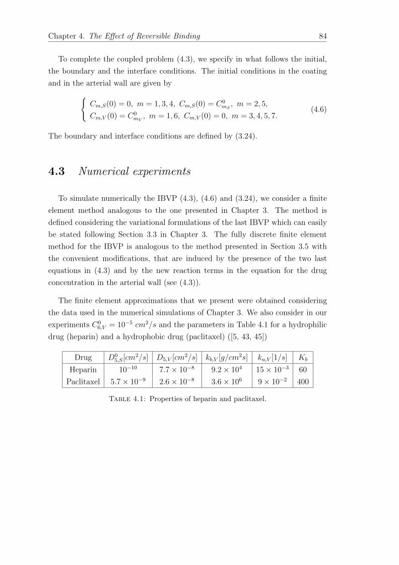
Chapter 4. The Effect of Reversible Binding 84
To complete the coupled problem (4.3), we specify in what follows the initial,
the boundary and the interface conditions. The initial conditions in the coating
and in the arterial wall are given byCm,S(0) = 0, m = 1, 3, 4, Cm,S(0) = C0
mS, m = 2, 5,
Cm,V (0) = C0mV, m = 1, 6, Cm,V (0) = 0, m = 3, 4, 5, 7.
(4.6)
The boundary and interface conditions are defined by (3.24).
4.3 Numerical experiments
To simulate numerically the IBVP (4.3), (4.6) and (3.24), we consider a finite
element method analogous to the one presented in Chapter 3. The method is
defined considering the variational formulations of the last IBVP which can easily
be stated following Section 3.3 in Chapter 3. The fully discrete finite element
method for the IBVP is analogous to the method presented in Section 3.5 with
the convenient modifications, that are induced by the presence of the two last
equations in (4.3) and by the new reaction terms in the equation for the drug
concentration in the arterial wall (see (4.3)).
The finite element approximations that we present were obtained considering
the data used in the numerical simulations of Chapter 3. We also consider in our
experiments C06,V = 10−5 cm2/s and the parameters in Table 4.1 for a hydrophilic
drug (heparin) and a hydrophobic drug (paclitaxel) ([5, 43, 45])
Drug D05,S[cm2/s] D5,V [cm2/s] kb,V [g/cm2s] ku,V [1/s] Kb
Heparin 10−10 7.7× 10⁻⁸ 9.2× 10⁴ 15× 10−3 60
Paclitaxel 5.7× 10⁻⁹ 2.6× 10⁻⁸ 3.6× 10⁶ 9× 10⁻² 400
Table 4.1: Properties of heparin and paclitaxel.

Chapter 4. The Effect of Reversible Binding 85
Figure 4.2: Distribution of heparin in the arterial wall in the models withoutbinding sites (top) and with binding sites (bottom) after 30 days.
Distribution of heparin in the arterial wall, with and without binding, after 30
days is plotted in Figure 4.2. Figure 4.3 illustrates the evolution of the mass of
heparin mass with and without binding. We remark that when binding occurs
the drug has a longer residence time in the arterial wall. We observe that the
concentration of drug in the arterial wall, when affinity between drug and living
tissue occurs, is higher than in the case of non affinity.
TaxusTM paclitaxel eluting stent from Boston Scientific, Natick, MA, USA,
applies paclitaxel, a fairly hyrophobic drug (Kb = 400), as a therapeutic agent

Chapter 4. The Effect of Reversible Binding 86
0 5 10 15 20 25 300
0.05
0.1
0.15
0.2
0.25
0.3
0.35
Time (Days)
Mas
s of
dru
g
Model without binding siteModel with binding site
Figure 4.3: Evolution of the mass of heparin in the arterial wall with andwithout binding sites during 30 days.
to control migration of smooth muscle cells from endothelium caused by in-stent
restenosis. Heparin, a hydrophobic drug (Kb = 60), is used in Carmeda BioActive
Surface (CBAS) heparin coating made by Carmeda, Upplands Vasby, Stockholm,
Sweden.
It should be noted that drugs like sirolimus (Kb = 1700), known also as
rapamycin, which is loaded in sirolimus eluting stent from Cordis, Johnson &
Johnson, Miami Lake, FL, USA, and also everolimus (Kb = 1700) loaded in
XIENCE V TM everolimus eluting stent manufactured by Abbott Vascular, Santa
Clara, CA, USA, are more hydrophobic than paclitaxel and are used to remain in
the arterial wall for a longer period.
Distribution of heparin and paclitaxel in the arterial wall after 30 days are illus-
trated in Figure 4.4, while the evolution of the masses of heparin and paclitaxel,
released from drug eluting stents in the arterial wall are compared in Figure 4.5.
We observe that resident time of paclitaxel is higher than of the heparin. This
means that heparin leaves the arterial wall faster than the paclitaxel.

Chapter 4. The Effect of Reversible Binding 87
Figure 4.4: Distribution of heparin (top) and paclitaxel (bottom) in the arte-rial wall after 30 days.
Evolution of paclitaxel in a healthy coronary artery with Young modulus κr =
1.2 MPa ([17]) is compared with a highly diseased coronary artery with Young
modulus κr = 4.1 MPa ([30]) in Figure 4.6. When κr increases due to age or
atherosclerosis, less drug penetrates to the coronary wall in the beginning of the
process. A crossing occurs around day 7. This result is justified by the fact that
the stiffness of the arterial wall imposes a resistance to the penetration of the drug
in the beginning of the process and leads to a drug accumulation in the long time.
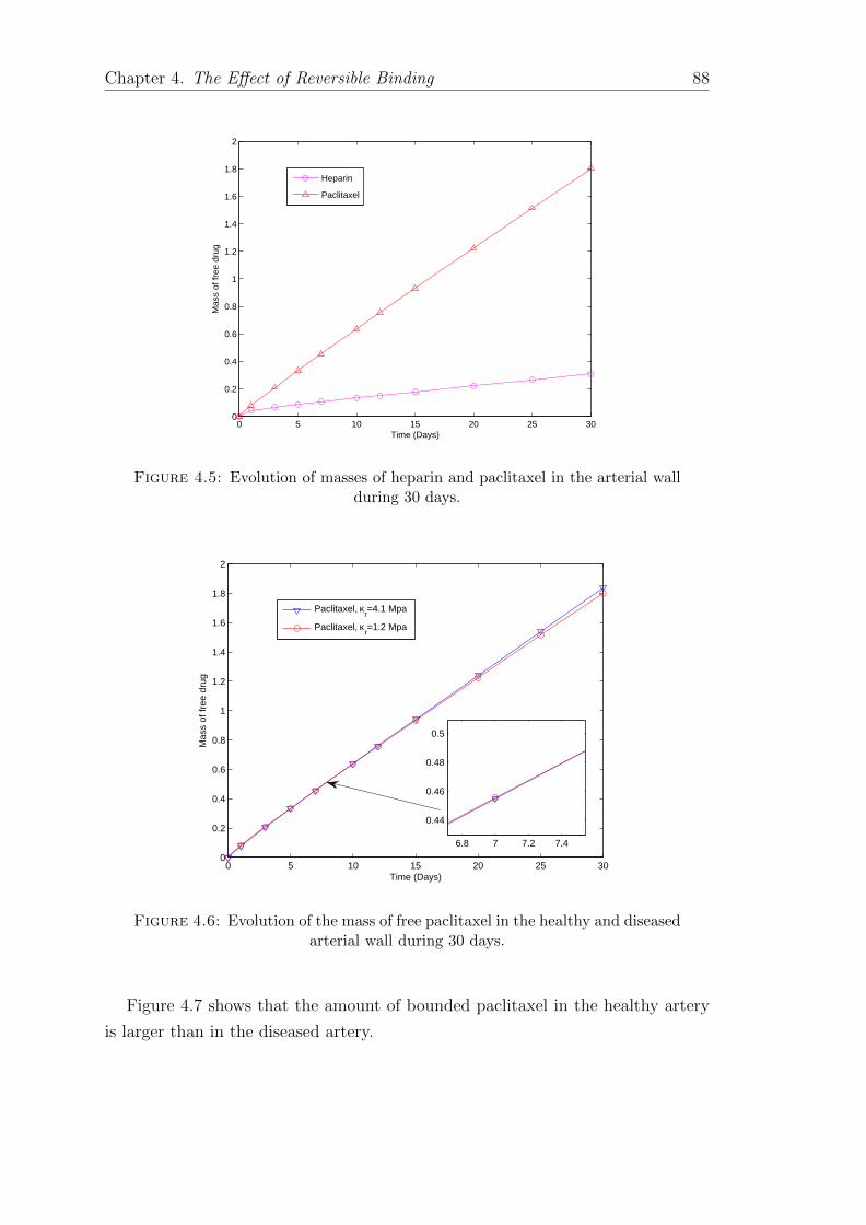
Chapter 4. The Effect of Reversible Binding 88
0 5 10 15 20 25 300
0.2
0.4
0.6
0.8
1
1.2
1.4
1.6
1.8
2
Time (Days)
Mas
s of
free
dru
g
Heparin
Paclitaxel
Figure 4.5: Evolution of masses of heparin and paclitaxel in the arterial wallduring 30 days.
0 5 10 15 20 25 300
0.2
0.4
0.6
0.8
1
1.2
1.4
1.6
1.8
2
Time (Days)
Mas
s of
free
dru
g
Paclitaxel, κr=4.1 Mpa
Paclitaxel, κr=1.2 Mpa
6.8 7 7.2 7.4
0.44
0.46
0.48
0.5
Figure 4.6: Evolution of the mass of free paclitaxel in the healthy and diseasedarterial wall during 30 days.
Figure 4.7 shows that the amount of bounded paclitaxel in the healthy artery
is larger than in the diseased artery.

Chapter 4. The Effect of Reversible Binding 89
0 5 10 15 20 25 300
0.5
1
1.5
2
2.5
x 10−10
Time (Days)
Mas
s of
bou
nded
dru
g
Paclitaxel, κr=4.1 Mpa
Paclitaxel, κr=1.2 Mpa
Figure 4.7: Evolution of the mass of bound paclitaxel in the healthy anddiseased arterial wall during 30 days.
In this chapter we studied the influence of reversible binding sites on the drug
release from a DES to an arterial wall. The mathematical model and the time
discrete finite element method used in the numerical simulations were obtained
modifying the mathematical model and the method of Chapter 3 to include binding
and unbinding effects. The numerical results highlight the difference between
the behaviour of a hydrophilic drug like heparin and a hydrophobic drug like
paclitaxel.


Chapter 5
Conclusions and Future Work
5.1 Conclusions
In this thesis we presented some coupled models to simulate the release of a
therapeutic agent from a drug eluting stent into the arterial wall. Different types
of interface and natural boundary conditions are taken into consideration based on
the physiological assumptions of the problem. The coating of the stent is assumed
to be biodegradable, viscoelastic properties of the arterial wall and affinity between
drug and vessel walls are considered in the complete model studied in Chapters
3 and 4 . From a theoretical viewpoint, appropriate variational formulations for
mathematical models have been introduced and energy estimates for the contin-
uous and fully discrete models have been established. We have introduced IMEX
finite element methods to solve the initial boundary value problems associated to
the system of equations of the models.
From the numerical viewpoint some particular aspects of clinical importance
such as sensitivity to the effective parameters that characterize the biodegradable
polymeric stent, the influence of the viscoelasticity of the arterial wall, the effect
of permeability of the stent coating and the effect of reversible binding reaction in
the release of different drugs are addressed in the thesis.
Regarding the biodegradable polymer, it is illustrated that the drug release from
a biodegradable stent is faster than the release of drug from a non-biodegradable
stent. This finding, which was obviously expected, has been quantified. We believe
that this quantification should be taken into consideration in the design of stents,
that is in the selection of the polymer and the initial concentration of drug.
91

Chapter 5. Conclusions and Future Work 92
Concerning the second clinical aspect, we showed that during an initial period
of time the permeation of the drug in the arterial wall is affected by its stiffness
i.e. the total mass of drug that enters into the arterial wall is a decreasing function
of the Young modulus. Patients who need a cardiovascular stent generally have
atherosclerosis and consequently stiffer arterial walls, that is they have higher
Young modulus. To prevent an inflammatory response and the smooth muscle
cell growth, a correct concentration of the drug must penetrate into the arterial
wall from the moment that the stent is implanted. Our findings suggest that the
initial concentration of the drug in the stent should be tailored to the rheological
properties of the arterial wall.
The third clinical aspect that we want to stress is the control of the release
profile according to the permeability of the coating: release can be speeded up or
delayed as different polymers are used. Application of different topcoats may alter
the penetration rate of the drug from the stent into the arterial wall.
Our last clinical finding is the effect of reversible binding reaction in the release
of different drugs. We observed that a hydrophobic drug such as paclitaxel stays
longer than a hydrophilic drug like heparin in the arterial wall. This result can
help to construct more effective drug eluting stents in the future.
Although our numerical results have been validated from a qualitative viewpoint
using data extracted from scientific works, by leading experts in the cardiovascular
drug delivery field, a comparison of the model with experimental results would
open new routes of research.
5.2 Future work
Viscoelastic properties of the polymeric stent
It is known that polymers like PLA exhibit viscoelastic properties influenced
by the degradation of the polymer into smaller molecules. In recent years several
models have been proposed to describe non-Fickian diffusion in polymers by in-
troducing viscoelastic properties ([6]). Much less attention has been devoted to
the mathematical modeling of viscoelasticity of the polymeric coating of the stent
in drug release.

Chapter 5. Conclusions and Future Work 93
We plan to address this problem in the near future by using appropriate linear
viscoelastic model such as Maxwell-Viechert Model. We believe this will open a
new research line to develop optimal design for drug eluting stents.
Bioabsorbable drug eluting stents
Recently some leading companies in the design of cardiovascular stents, such
as Abbott Vascular, Santa Clara, CA, USA, and Boston Scientific, Natick, MA,
USA, have started to design a new generation of drug eluting stents named bioab-
sorbable stents. This type of stent is mostly made by completely bioabsorbable
polymers with stent strut made by biocompatible metals like magnesium, iron or
other alloys. These metals are resorbed from the body after around three months,
which corresponds to the most critical period after stent implantation. In current
biodegradable DES, manufacturers use metals like titanium or chromium which
are not metabolized by the body. This fact have several drawbacks as for example
causing a late stent thrombosis.
ABSORB which has been recently launched by Abbott Vascular is a biore-
sorbable vascular scaffold system that elutes everolimus in a similar way to the
drug eluting stent XIENCE V TM and then is naturally resorbed leaving no perma-
nent scaffold. ABSORB is composed of four key design elements: a bioresorbable
scaffold (Poly (L-lactide)), a bioresorbable coating (poly (D,L lactide)), everolimus
and the XIENCE V TM delivery system.
To model this next generation of stents, new reaction equations and modified
interface and boundary conditions are needed. To the best of our knowledge,
mathematical modeling, numerical and theoretical studies of this kind of stents
have not been yet in the literature. We plan to model, in the time coming, drug
delivery from ABSORB into a viscoelastic vessel.


Bibliography
[1] S. D. Abramowitch and S. L.-Y. Woo, A new analytical approach to
evaluate the viscoelastic properties of the goat medial collateral ligament using
the quasilinear viscoelastic theory, Proceedings of the Summer Bioengineering
Conference, ASME, Key Biscayne, Florida, (2003), pp. 47–92.
[2] G. Acharya and K. Park, Mechanisms of controlled drug release from
drug-eluting stents, Advanced Drug Delivery Reviews, 58 (2006), pp. 387–
401.
[3] R. Adams and J. Fournier, Sobolev Spaces, Elsevier 2nd edition, 2003.
[4] D. Boffi, F. Brezzi, and M. Fortin, Mixed Finite Element Methods and
Applications, Springer Series in Computational Mathematics, Vol 44, 2013.
[5] A. Borghi, E. Foa, R. Balossino, F. Migliavacca, and G. Dubini,
Modelling drug elution from stents: effects of reversible binding in the vascular
wall and degradable polymeric matrix, Computer Methods in Biomechanics
and Biomedical Engineering, 11 (2008), pp. 367–377.
[6] H. F. Brinson and L. C. Brinson, Polymer Engineering Science and
Viscoelasticity: An Introduction, Springer, 2010.
[7] Z. Chen, G. Huan, and Y. Ma, Computational Methods for Multiphase
Flows in Porous Media, Computational Science and Engineering, SIAM, 2006.
[8] D. Cohen and A. B. White, Jr., Sharp fronts due to diffusion and vis-
coelastic relaxation in polymers, SIAM Journal on Applied Mathematics, 51
(1991), pp. 472–483.
[9] J. Crank and G. S. Park, Diffusion in Polymers, Academic Press, 1968.
[10] D. A. Edwards and D. S. Cohen, A mathematical model for a dissolving
polymer, AIChE Journal, 41 (1995), pp. 2345–2355.
95
Bibliography 96
[11] L. C. Evans, Partial Differential Equations, American Mathematical Soci-
ety, 1998.
[12] J. A. Ferreira, P. de Oliveira, and P. M. Silva, Reaction–diffusion in
viscoelastic materials, Journal of Computational and Applied Mathematics,
236 (2012), pp. 3783–3795.
[13] J. A. Ferreira, M. Grassi, E. Gudino, and P. de Oliveira, A 3D
Model for Mechanistic Control of Drug Release, SIAM Journal on Applied
Mathematics, 74 (2014), pp. 620–633.
[14] J. A. Ferreira, M. Grassi, E. Gudino, and P. de Oliveira, A new
look to non-Fickian diffusion, Applied Mathematical Modelling, 39 (2015),
pp. 194–204.
[15] J. A. Ferreira, E. Gudino, and P. de Oliveira, Analytical and Numer-
ical Study of Memory Formalisms in Diffusion Processes, Modelling and Sim-
ulation in Fluid Dynamics in Porous Media, Springer Proceedings in Mathe-
matics and Statistics, J. A. Ferreira, S. Barbeiro, G. Pena and M. F. Wheeler
(editors), 28 (2013), pp. 67–85.
[16] Y. C. Fung, Biomechanics: Mechanical Properties of Living Tissues,
Springer-Verlag, 1993.
[17] B. S. Gow and C. D. Hadfield, The elasticity of canine and human
coronary arteries with reference to postmortem changes, Circulation Research,
45 (1979), pp. 588–594.
[18] M. Grassi, G. Pontrelli, L. Teresi, G. Grassi, L. Comel, A. Fer-
luga, and L. Galasso, Novel design of drug delivery in stented arteries:
a numerical comparative study, Mathematical Biosciences and Engineering, 6
(2009), pp. 493–508.
[19] F. Hecht, freeFEM++, Third Edition, Version 3.20, tech. report.
[20] T. Khamdaeng, J. Luo, J. Vappou, P. Terdtoon, and E. E.
Konofagou, Arterial stiffness identification of the human carotid artery us-
ing the stress-strain relationship in vivo, Ultrasonics, 52 (2012), pp. 402–411.
[21] M. Kohandel, S. Sivaloganathan, and G. Tenti, Estimation of the
quasi-linear viscoelastic parameters using a genetic algorithm, Mathematical
and Computer Modelling, 47 (2008), pp. 266–270.

Bibliography 97
[22] Q. Liu and D. Kee, Modeling of diffusion through polymeric membranes,
Rheologica Acta, 44 (2004), pp. 287–294.
[23] Q. Liu, X. Wang, and D. De Kee, Mass transport through swelling mem-
branes, International Journal of Engineering Science, 43 (2005), pp. 1464–
1470.
[24] F. Migliavacca, F. Gervaso, M. Prosi, P. Zunino, S. Minisini,
L. Formaggia, and G. Dubini, Expansion and drug elution model of a
coronary stent, Computer Methods in Biomechanics and Biomedical Engi-
neering, 10 (2007), pp. 63–73.
[25] F. Migliavacca, L. Petrini, V. Montanari, I. Quagliana, F. Au-
ricchio, and G. Dubini, A predictive study of the mechanical behaviour of
coronary stents by computer modelling, Medical Engineering & Physics, 27
(2005), pp. 13–18.
[26] S. Minisini, Mathematical and Numerical Modeling of Controlled drug re-
lease, PhD thesis, Politecnico di Milano, 2009.
[27] A. Muliana and K. R. Rajagopal, Changes in the response of viscoelastic
solids to changes in their internal structure, Acta Mechanica, 217 (2010),
pp. 297–316.
[28] A. H. Muliana and K. R. Rajagopal, On the response of viscoelas-
tic biodegradable polymeric solids, Mechanics Research Communications, 39
(2012), pp. 51–58.
[29] A. Nekouzadeh, K. M. Pryse, E. L. Elson, and G. M. Genin, A
simplified approach to quasi-linear viscoelastic modeling, Journal of Biome-
chanics, 40 (2007), pp. 3070–3078.
[30] I. Ozolanta, G. Tetere, B. Purinya, and V. Kasyanov, Changes
in the mechanical properties, biochemical contents and wall structure of the
human coronary arteries with age and sex, Medical Engineering & Physics,
20 (1998), pp. 523–533.
[31] G. Pontrelli, The role of the arterial prestress in blood flow dynamics,
Medical Engineering & Physics, 28 (2006), pp. 6–12.
[32] G. Pontrelli and F. de Monte, Mass diffusion through two-layer porous
media: an application to the drug-eluting stent, International Journal of Heat
and Mass Transfer, 50 (2007), pp. 3658–3669.

Bibliography 98
[33] , A multi-layer porous wall model for coronary drug-eluting stents, Inter-
national Journal of Heat and Mass Transfer, 53 (2010), pp. 3629–3637.
[34] S. Prabhu and S. Hossainy, Modeling of degradation and drug release
from a biodegradable stent coating, Journal of Biomedical Materials Research.
Part A, 80 (2007), pp. 732–741.
[35] A. Raval, J. Parikh, and C. Engineer, Mechanism of controlled release
kinetics from medical devices, Brazilian Journal of Chemical Engineering, 27
(2010), pp. 211–225.
[36] J. N. Reddy, An Introduction to the Finite Element Method, McGraw-Hill;
3rd edition, 2005.
[37] J. M. Schakenraad, M. J. Hardonk, J. Feijen, I. Molenaar, and
P. Nieuwenhuis, Enzymatic activity toward poly(L-lactic acid) implants,
Journal of Biomedical Materials Research, 24 (1990), pp. 529–545.
[38] J. Siepmann and A. Gopferich, Mathematical modeling of bioerodible,
polymeric drug delivery systems, Advanced Drug Delivery Reviews, 48 (2001),
pp. 229–247.
[39] J. S. Soares, Constitutive Modeling for Biodegradable Polymers Application
in Endovascular Stents, PhD thesis, Mechanical Engineering, Texas A&M
University, 2008.
[40] J. S. Soares, J. E. Moore, and K. R. Rajagopal, Modeling of defor-
mation accelerated breakdown of polylactic acid biodegradable stents, Journal
of Medical Devices, 4 (2010), p. 41007.
[41] Y. Tao, Nonlinear Viscoelastic Properties and Constitutive Modeling of Blood
Vessel, Master’s thesis, National University of Singapore, 2009.
[42] K. L. Troyer, D. Estep, and C. M. Puttlitz, Viscoelastic effects dur-
ing loading play an integral role in soft tissue mechanics, Acta Biomaterialia,
8 (2012), pp. 234–243.
[43] V. Tuoi, Mathematical Analysis of Some Models for Drug Delivery, PhD
thesis, National University of Ireland, 2012.
[44] C. Vergara and P. Zunino, Multiscale boundary conditions for drug re-
lease from cardiovascular stents, Multiscale Modeling & Simulation, 7 (2008),
pp. 565–588.

Bibliography 99
[45] F. Zhang, M. Fath, R. Marks, and R. Linhardt, A highly stable co-
valent conjugated heparin biochip for heparin-protein interaction studies, An-
alytical Biochemistry, 304 (2002), pp. 271–273.
[46] P. Zunino, Multidimensional pharmacokinetic models applied to the design
of drug-eluting stents, Cardiovascular Engineering, 4 (2004), pp. 181–191.