Non-Equilibrium Statistical Mechanicspavl/noneqstatmech.pdf · Non-Equilibrium Statistical...

Non-Equilibrium Statistical Mechanics

G.A. PavliotisDepartment of Mathematics

Imperial College LondonLondon SW7 2AZ, UK

June 20, 2012

Contents

1 Derivation of the Langevin Equation 11.1 Open Classical Systems . . . . . . . . . . . . . . . . . . . . . . . 11.2 The Markovian Approximation . . . . . . . . . . . . . . . . . . . 81.3 Derivation of the Langevin Equation . . . . . . . . . . . . . . . . 131.4 Discussion and Bibliography . . . . . . . . . . . . . . . . . . . . 151.5 Exercises . . . . . . . . . . . . . . . . . . . . . . . . . . . . . . 16

2 Linear Response Theory for Diffusion Processes 192.1 Linear Response Theory . . . . . . . . . . . . . . . . . . . . . . 192.2 The Fluctuation–Dissipation Theorem . . . . . . . . . . . . . . .252.3 Einstein’s Relation and the Green-Kubo Formula . . . . . . .. . 282.4 Discussion and Bibliography . . . . . . . . . . . . . . . . . . . . 312.5 Exercises . . . . . . . . . . . . . . . . . . . . . . . . . . . . . . 32

i

ii CONTENTS

Chapter 1

Derivation of the LangevinEquation

In this chapter we derive the Langevin equation from a simplemechanical modelfor a small system (that we will refer to as the Brownian particle) that is in con-tact with a thermal reservoir which is at thermodynamic equilibrium at timet =

0. The full Brownian particle plus thermal reservoir dynamics is assumed to beHamiltonian. The derivation proceeds in three steps. First, we derive a closedstochastic integrodifferential equation for the dynamicsof the Brownian particle,the Generalized Langevin Equation (GLE) . In the second step, we approximatethe GLE by a finite dimensional Markovian equation in an extended phase space.Finally, we use singular perturbation theory for Markov processes to derive theLangevin equation, under the assumption of rapidly decorrelating noise. Thisderivation provides a partial justification for the use of stochastic differential equa-tions, in particular, the Langevin equation, in the modeling of physical systems.

In Section 1.1 we study a simple model for open classical systems and wederive the Generalized Langevin Equation. The Markovian approximation of theGLE is studied in Section 1.2. The derivation of the Langevinequation from thisMarkovian approximation is studied in Section 1.3. Discussion and bibliographicalremarks are included in Section 1.4. Exercises can be found in Section 1.5.

1.1 Open Classical Systems

We consider a particle in one dimension that is in contact with a thermal reservoir(heat bath), a system with infinite heat capacity at temperatureβ−1 that interacts

1

2 CHAPTER 1. DERIVATION OF THE LANGEVIN EQUATION

(exchanges energy) with the particle. We will model the reservoir as a system ofinfinitely many non-interacting particles which is in thermodynamic equilibriumat time t = 0. In other words, we will model the heat bath as a system of in-finitely many harmonic oscillators whose initial energy is distributed according tothe canonical (Boltzmann-Gibbs) distribution at temperatureβ−1.

A finite collection of harmonic oscillators is a Hamiltoniansystem with Hamil-tonian

H(p,q) =1

2

N∑

j=1

p2j +

1

2

N∑

j=1

q2j , (1.1)

where for simplicity we have set all the spring constants{kj}Nj=1 equal to1. The

corresponding canonical distribution is

µβ(dp, dq) =1

Ze−βH(p,q) dpdq. (1.2)

Since the Hamiltonian (1.1) is quadratic in both positions and momenta, the mea-sure (1.2) is Gaussian. We setz = (q, p) ∈ R

2N =: H and denote by〈·, ·〉the Euclidean inner product in (the Hilbert space)H. Then, for arbitrary vectorsh, b ∈ H we have

E〈z,h〉 = 0, E

(〈z,h〉〈z,b〉

)= β−1〈h,b〉. (1.3)

We want to consider an infinite dimensional extension of the above model for theheat bath. A natural infinite dimensional extension of a finite system of harmonicoscillators is the wave equation∂2

t ϕ = ∂2xϕ that we write as a system of equations

∂tϕ = π, ∂tπ = ∂2xϕ. (1.4)

The wave equation is an infinite dimensional Hamiltonian system with Hamiltonian

H(π, ϕ) =1

2

∫

R

(|π|2 + |∂xϕ|2

)dx. (1.5)

It is convenient to introduce the Hilbert spaceHE with the (energy) norm

‖φ‖2 =

∫

R

(|π|2 + |∂xϕ|2

)dx (1.6)

whereφ = (ϕ, π). The corresponding inner product is

〈φ1, φ2〉 =

∫

R

(∂xϕ1(x)∂xϕ2(x) + π1(x)π2(x)

)dx (1.7)

1.1. OPEN CLASSICAL SYSTEMS 3

where the overbar denotes the complex conjugate. Using the notation (1.6) we canwrite the Hamiltonian for the wave equation as

H(φ) =1

2‖φ‖2.

We would like to extend the Gibbs distribution (1.2) to this infinite dimensionalsystem. However, the expression

µβ(dπdϕ) =1

Ze−βH(ϕ,π)Πx∈R dπdϕ (1.8)

is merely formal, since Lebesgue measure does not exist in infinite dimensions.However, this measure is Gaussian (the HamiltonianH is a quadratic functional inπ andφ) and the theory of Gaussian measures in Hilbert spaces is well developed.This theory goes beyond the scope of this book1 For our purposes it is sufficient tonote that ifX is a Gaussian random variable in the Hilbert spaceHE with innerproduct (1.7) then〈X, f〉 is a scalar Gaussian random variable with mean andvariance

〈X, f〉 = 0, and E

(〈X, f〉〈X,h〉

)= β−1〈f, h〉. (1.9)

Notice the similarity between the formulas in (1.3) and (1.9).We assume that the full dynamics of the particle coupled to the heat bath is

Hamiltonian described by a Hamiltonian function

H(p, q, π, ϕ) = H(p, q) + HHB(π, ϕ) +HI(q, ϕ). (1.10)

We useHHB(π, φ) to denote the Hamiltonian for the wave equation (1.5).H(p, q)

denotes the Hamiltonian of the particle, whereasHI describes the interaction be-tween the particle and the fieldφ. We assume that the coupling is only through thepositionq andφ, it does not depend on the momentump and the momentum fieldπ.We assume that the particle is moving in a confining potentialV (q). Consequently:

H(p, q) =p2

2+ V (q). (1.11)

Concerning the coupling, we assume that it is linear in the field φ and that it istranslation invariant:

HI(q, ϕ) =

∫

R

ϕ(x)ρ(x − q) dx. (1.12)

1Some discussion about Gaussian measures in Hilbert spaces can be found in Section??.


The coupling between the particle and the heat bath depends crucially on the func-tion ρ(x) which is arbitrary at this point.2

Now we make an approximation that will simplify considerably the analysis:since the particle moves in a confining potential (think of a quadratic potential),we can assume that its position does not change too much. Consequently, we canperform a Taylor series expansion in (1.12) which, togetherwith an integration byparts gives (see Exercise 1)3

HI(q, ϕ) ≈ q

∫

R

∂xϕ(x)ρ(x) dx. (1.13)

The coupling now is linear in bothq andϕ. This will enable us to integrate outexplicitly the fieldsϕ andπ from the equations of motion and to obtain a closedequation for the dynamics of the particle.

Putting (1.11), (1.5) and (1.13) together, the Hamiltonian(1.10) becomes

H(p, q, π, φ) =p2

2+ V (q) +

1

2

∫

R

(|π|2 + |∂xϕ|2

)dx+ q

∫

R

∂xϕ(x)ρ(x) dx.

(1.14)Now we can derive Hamilton’s equations of motion for the coupled particle-fieldmodel (1.14):

q =∂H∂p

, p = −∂H∂q

, (1.15a)

∂tϕ =δHδπ

, ∂tπ = −δHδϕ

, (1.15b)

where δHδ· stands for the functional derivative.4 Carrying out the differentiations

we obtain

q = p, p = −V ′(q) −∫

R

∂xϕ(x)ρ(x) dx, (1.16a)

∂tϕ = π, ∂tπ = ∂2xϕ+ q∂xρ. (1.16b)

Our goal now is to solve equations (1.16b), which is a system of linear inhomo-geneous differential equations and then substitute into (1.16a). We will use the

2In the terminology of electrodynamics,ρ plays the role of acharge density.3Again, in the terminology of electrodynamics this is calledthedipole approximation.4We remind the reader that for a functional of the formH(φ) =

R

RH(φ, ∂xφ) dx the functional

derivative is given byδHδφ

= ∂H∂φ

−∂

∂x∂H

∂(∂xρ). We apply this definition to the functional (1.14) to

obtain δHδπ

= π, δHδϕ

= −∂2xϕ − q∂xρ.


variation of constants formula (Duhamel’s principle). It is more convenient torewrite (1.16) in a slightly different form. First, we introduce the operator

A =

(0 1∂2

x 0

), (1.17)

acting on functions inHE with inner product (1.7). It is not hard to show that theA is an antisymmetric operator in this space (see Exercise 2).Furthermore, weintroduce the notationα = (α1(x), 0) ∈ HE with ∂xα1(x) = ρ(x). Noticing that

Aα = (0, ∂xρ),

we can rewrite (1.16b) in the form

∂tφ = A(φ+ qα) (1.18)

with φ = (ϕ, π). Furthermore, the second equation in (1.16) becomes

p = −V ′(q) − 〈φ, α〉. (1.19)

Finally, we introduce the functionψ = φ+ qα to rewrite

∂tψ = Aψ + pα. (1.20)

Similarly, we introduceψ in (1.19) to obtain

p = −V ′eff (q) − 〈ψ,α〉, (1.21)

whereVeff (q) = V (q) − 1

2‖α‖2q2. (1.22)

Notice that‖α‖2 = ‖ρ‖2

L2 =: λ.

The parameterλ measures the strength of the coupling between the particle andthe heat bath. The correction term in the potentialVeff (q) is essentially due to theway we have chosen to write the equations of motion for the particle-field systemand it is not fundamental; see Exercise 1.

The solution of (1.20) is

ψ(t) = eAtψ(0) +

∫ t

0eA(t−s)p(s)α ds.


We substitute this in (1.21) to obtain

p = −V ′eff (q) − 〈ψ,α〉

= −V ′eff (q) −

⟨eAtψ(0), α

⟩−∫ t

0

⟨eA(t−s)α,α

⟩p(s) ds

= −V ′eff (q) −

∫ t

0γ(t− s)p(s) ds+ F (t)

whereF (t) =

⟨ψ(0), e−Atα

⟩(1.23)

andγ(t) =

⟨e−Atα,α

⟩(1.24)

Notice thatψ(0) = φ(0) + q(0)α is a Gaussian field with mean and covariance,using (1.9),

E〈ψ(0), f〉 = q(0)〈α, f〉 =: µf

andE ((〈ψ(0), f〉 − µf ) (〈ψ(0), h〉 − µh)) = β−1〈f, h〉.

To simplify things we will setq(0) = 0. ThenF (t) is a mean zero stationaryGaussian process with autocorrelation function

E(F (t)F (s)) = E(⟨ψ(0), e−Atα

⟩ ⟨ψ(0), e−Asα

⟩)

= β−1⟨e−Atα, e−Asα

⟩

= β−1γ(t− s),

where we have used (1.9). Consequently, the autocorrelation function of the stochas-tic forcing in (1.23) is precisely the kernel (times the temperature) of the dissipationterm in the equation forp. This is an example of thefluctuation-dissipation theo-rem .

To summarize, we have obtained a closed equation for the dynamics of theparticle, theGeneralized Langevin Equation

q = −V ′eff (q) −

∫ t

0γ(t− s)q(s) ds + F (t), (1.25)

with F (t) being a mean zero stationary Gaussian processes with autocorrelationfunction given by the fluctuation–dissipation theorem

E(F (t)F (s)) = β−1γ(t− s). (1.26)


It is clear from formula (1.24) and the definition ofα that the autocorrelation func-tion γ(t) depends only on the densityρ.5 In fact, we can show that (see Exercise 3)that

γ(t) =

∫

R

|ρ(k)|2eiktdk, (1.27)

whereρ(k) denotes the Fourier transform ofρ.Let us now make several remarks on the Generelized Langevin Equation (1.25)

(GLE). First, notice that the GLE is Newton’s equation of motion for the particle,augmented with two additional terms: a linear dissipation term which depends onthe history of the particle position and a stochastic forcing term which is relatedto the the dissipation term through the fluctuation–dissipation theorem (1.26). Thefact that the fluctuations (noise) and the dissipation in thesystems satisfy such arelation is not surprising, since they have the same source,namely the interactionbetween the particle and the field. Is is important to note that the noise (and also thefact that it is Gaussian and stationary) in the GLE is due to our assumption that theheat bath is at equilibirum at timet = 0, i.e. that the initial equations of the waveequation are distributed according to the (Gaussian) Gibbsmeasure (1.8). Perhapssurprisingly, the derivation of the GLE and the fluctuation dissipation theorem arenot related to our assumption that the heat bath is describedby a field, i.e. itis a dynamical system with infinitely many degrees of freedom. We could havearrived at the GLE and the fluctuation–dissipation theorem even if we had onlyone oscillator in the “heat bath”. See Exercise 6.

Furthermore, the autocorrelation function of the noise depends only on thecoupling functionρ(x): different choices of the coupling function lead to differentnoise processesF (t). 6

It is also important to emphasize the fact that the GLE (1.25)isequivalentto theoriginal Hamiltonian dynamics (1.14) with random initial conditions distributedaccording to (1.8). So far, no approximation has been made. We have merely usedthe linearity of the dynamics of the heat bath and the linearity of the coupling inorder to integrate out the heat bath variables by using the variation of constantsformula.

Finally we remark that an alternative way for writing the GLEis

q = −V ′(q) −∫ t

0D(t− s)q(s) ds+ F (t) (1.28)

5Assuming, of course, that the heat bath is described by a waveequation, i.e. assuming thatA isthe wave operator.

6In fact, the autocorrelation function depends also on the operatorA in (1.17).


with

D(t) = 〈AeAtα,α〉. (1.29)

The fluctuation-dissipation theorem takes the form

γ(t) = D(t). (1.30)

See Exercise 7. When writing the GLE in the form (1.28) there is no need tointroduce an effective potential or to assume thatq(0) = 0.

1.2 The Markovian Approximation

From now on we will ignore the correction in the potential (1.22). We rewrite theGLE (1.25):

q = −V ′(q) −∫ t

0γ(t− s)q(s) ds + F (t), (1.31)

together with the fluctuation-dissipation theorem (1.26).Equation (1.31) is a non-Markovian stochastic equation, since the solution at timet depends on the entirepast. In this section we show that when autocorrelation function γ(t) decays suf-ficiently fast, then the dynamics of the particle can be described by a Markoviansystem of stochastic differential equations in an extendedphase space. The basicobservation that was already made in Chapter??, Exercise?? that a one dimen-sional mean zero Gaussian stationary with continuous pathsand an exponentialautocorrelation function is necessarily the Ornstein-Uhlenbeck process. This isthe content of Doob’s theorem . Consequently, if the memory kernel (autocorre-lation function)γ(t) is decaying exponentially fast, then we expect that we candescribe the noise in the GLE by adding a finite number of auxiliary variables.We can formalize this by introducing the concept of aquasi-Markovian processquasi-Markovian process:

Definition 1.1. We will say that a stochastic processXt is quasi-Markovian if itcan be represented as a Markovian stochastic process by adding a finite number ofadditional variables: there exists a finite dimensional stochastic processYt so that{Xt, Yt} is a Markov process.

In the following result we will use the notation〈·, ·〉 to denote the Euclideaninner product.

1.2. THE MARKOVIAN APPROXIMATION 9

Proposition 1.2. Let λ ∈ Rd, A ∈ R

d×d, positive definite, and assume that theautocorrelation functionγ(t) is given by

γ(t) = 〈e−Atλ, λ〉. (1.32)

Then the GLE(1.31)is equivalent to the SDE

q(t) = p(t), (1.33a)

p(t) = −V ′(q(t)) + 〈λ, z(t)〉, (1.33b)

z(t) = −p(t)λ−A z(t) + ΣW (t), z(0) ∼ N (0, β−1I), (1.33c)

wherez : R+ 7→ R

m, λ ∈ Rm, Σ ∈ R

m×m and the matrixΣ satisfies

ΣΣT = β−1(A+AT ). (1.34)

Remark 1.3. Notice that the formula for the autocorrelation function(1.32) issimilar to (1.24). However, the operatorA in (1.24) is the wave operator(1.17),i.e. the generator of a unitary group, whereas the operatorA (or, rather,−A) thatappears in(1.32)is the generator of the contraction semigroupe−At, i.e. a dissipa-tive operator. The source of the noise in(1.25)and in(1.33)is quite different, eventhough the have the same effect, when the autocorrelation function is exponentiallydecaying.

Proof. The solution of (1.33c) is

z(t) = e−Atz(0) +

∫ t

0e−A(t−s)ΣdW (s) −

∫ t

0e−A(t−s)λp(s) ds. (1.35)

We substitute this into (1.33b) to obtain

p = −V ′(q) −∫ t

0γ(t− s)p(s) ds + F (t)

withγ(t) = 〈e−Atλ, λ〉

and

F (t) =

⟨λ, e−Atz(0) +

∫ t

0e−A(t−s)ΣdW (s)

⟩

=: 〈λ, y(t)〉 ,


where

y(t) = S(t)z(0) +

∫ t

0S(t− s)ΣdW (s)

with S(t) = e−At. With our assumptions onZ(0) and (1.34),y(t) is a mean zerostationary Gaussian process with covariance matrix

Q(t− s) = E(yT (t)y(s)) = β−1S(|t− s|). (1.36)

To see this we first note that (using the summation convention)

E(yi(t)yj(s)) = Siℓ(t)Sjρ(t)E(zℓ(0)zρ(0)) +

∫ t

0

∫ s

0Siρ(t− ℓ)ΣρkSjn(s − τ)Σnkδ(ℓ− τ) dℓdm

= β−1Siρ(t)Sjρ(s) +

∫ min(t,s)

0Siρ(t− τ)ΣρkΣnkSjn(s− τ) dτ.

Consequently, and using (1.34),

E(yT (t)y(s)) = β−1S(t)ST (s) +

∫ min(t,s)

0S(t− τ)ΣT ΣST (s− τ) dτ

= β−1S(t)

(I +

∫ min(t,s)

0S(−τ)(A+AT )ST (−τ) dτ

)ST (s).

Without loss of generality we may assume thats 6 t. Now we claim that(I +

∫ min(t,s)

0S(−τ)(A+AT )ST (−τ) dτ

)ST (s) = S(−s).

To see this, notice that this equation is equivalent to

I +

∫ t,s

0S(−τ)(A +AT )ST (−τ) dτ = S(s)ST (−s).

This equation is clearly valid ats = 0. We differentiate to obtain the identity

S(−s)(A+AT )ST (−s) =d

dtS(s)ST (−s),

which is true for alls. This completes the proof of (1.36). Now we calculate, withs 6 t,

E(F (t)F (s)) = E (〈λ, y(t)〉〈λ, y(s)〉)= 〈Q(t− s)λ, λ〉 = β−1〈e−Atλ, λ〉= β−1γ(t− s)

and the proposition is proved.

1.2. THE MARKOVIAN APPROXIMATION 11

Example 1.4. Consider the casem = 1. In this case the vectorλ and the matrixA become scalar quantities. The SDE(1.33)becomes

q(t) = p(t),

p(t) = −V ′(q(t)) + λz(t),

z(t) = −λp(t) − αz(t) +√

2αβ−1W (t), z(0) ∼ N (0, β−1).

The autocorrelation function is

γ(t) = λ2e−αt.

Example 1.5. Consider now the case

A =

(0 11 −γ

).

The Markovian GLE takes the form

q = p, (1.37a)

p = −V ′(q) + 〈λ, z〉, (1.37b)

z1 = (z2 + λ1p), (1.37c)

z2 = (−z1 − γz2 − λ2p) +√

2β−1α2 W . (1.37d)

The generator of the dynamics (1.33) is

L = p∂q − ∂qV ∂p + 〈λ, z〉∂p − pλ · ∇z −Az · ∇z +1

2β−1A : Dz, (1.38)

whereA : Dz denotes the Frobenius inner product betweenA and the Hessian withrespect toz, A : Dz =

∑di,j=1Aij

∂2

∂zi∂zj.7 The Fokker-Planck operator is

L∗ = −p∂q + ∂qV ∂p − 〈λ, z〉∂p + pλ · ∇z + ∇z (Az· ) +1

2β−1A : Dz. (1.39)

When the potentialV (q) is confining then the processX(t) := (q(t), p(t), z(t))

has nice ergodic properties. We recall that the Hamiltonianof the system isH(p, q) =12p

2 + V (q).

7In fact, the last term in (1.38) should readβ−1As : Dz , whereAs = 12(A + AT ) denotes the

symmetric part ofA. However sinceDz is symmetric we can write it in the form12β−1A : Dz .


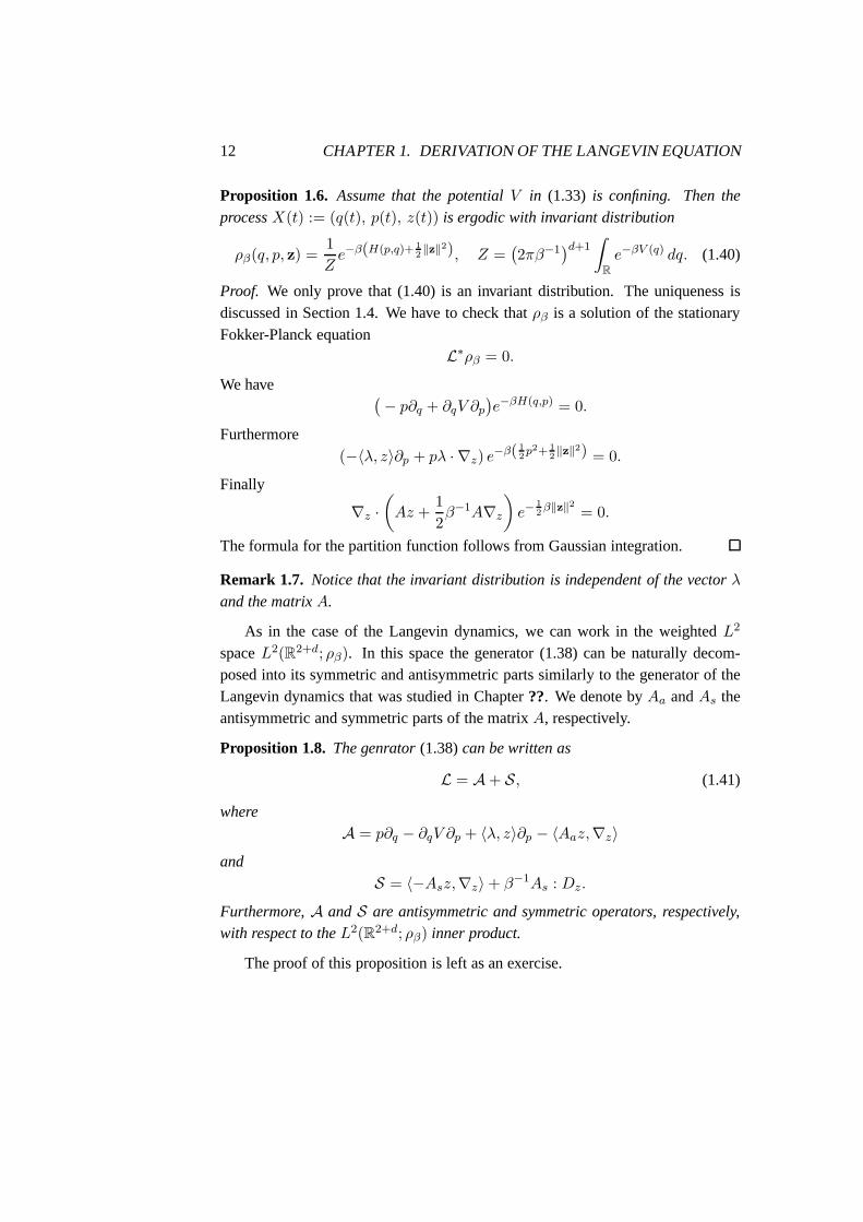
Proposition 1.6. Assume that the potentialV in (1.33) is confining. Then theprocessX(t) := (q(t), p(t), z(t)) is ergodic with invariant distribution

ρβ(q, p, z) =1

Ze−β(H(p,q)+ 1

2‖z‖2), Z =

(2πβ−1

)d+1∫

R

e−βV (q) dq. (1.40)

Proof. We only prove that (1.40) is an invariant distribution. The uniqueness isdiscussed in Section 1.4. We have to check thatρβ is a solution of the stationaryFokker-Planck equation

L∗ρβ = 0.

We have (− p∂q + ∂qV ∂p

)e−βH(q,p) = 0.

Furthermore(−〈λ, z〉∂p + pλ · ∇z) e

−β( 12p2+ 1

2‖z‖2) = 0.

Finally

∇z ·(Az +

1

2β−1A∇z

)e−

12β‖z‖2

= 0.

The formula for the partition function follows from Gaussian integration.

Remark 1.7. Notice that the invariant distribution is independent of the vectorλand the matrixA.

As in the case of the Langevin dynamics, we can work in the weightedL2

spaceL2(R2+d; ρβ). In this space the generator (1.38) can be naturally decom-posed into its symmetric and antisymmetric parts similarlyto the generator of theLangevin dynamics that was studied in Chapter??. We denote byAa andAs theantisymmetric and symmetric parts of the matrixA, respectively.

Proposition 1.8. The genrator(1.38)can be written as

L = A + S, (1.41)

whereA = p∂q − ∂qV ∂p + 〈λ, z〉∂p − 〈Aaz,∇z〉

andS = 〈−Asz,∇z〉 + β−1As : Dz.

Furthermore,A andS are antisymmetric and symmetric operators, respectively,with respect to theL2(R2+d; ρβ) inner product.

The proof of this proposition is left as an exercise.

1.3. DERIVATION OF THE LANGEVIN EQUATION 13

1.3 Derivation of the Langevin Equation

Now we are ready to derive the Langevin equation

q = p, p = −V ′(q) − γp+√

2γβ−1W , (1.42)

and to obtain a formula for the friction coefficientγ. We can derive the dynam-ics (1.42) from the GLE (1.31) in the limit where the correlation time of the noisebecomes very small,γ(t) → δ(t). This corresponds to taking the coupling in thefull Hamiltonian dynamics (1.14) to be localized,ρ(x) → δ(x).

We focus on the Markovian approximation (1.33) with the family of autocor-relation functions

γε(t) =1

ε2〈e−

A

ε2tλ, λ〉.

This corresponds to rescalingλ andA in (1.33) according toλ 7→ λ/ε andA 7→A/ε2. Equations (1.33) become

qε(t) = pε(t), (1.43a)

pε(t) = −V ′(qε(t)) +1

ε〈λ, zε(t)〉, (1.43b)

zε(t) = −1

εpε(t)λ− 1

ε2A zε(t) +

1

εΣW (t), zε(0) ∼ N (0, β−1I),(1.43c)

where (1.34) has been used.

Proposition 1.9. Let{qε(t), pε(t), zε(t)

}denote the solution of(1.43) and as-

sume that the matrixA is invertible. Then{qε(t), pε(t)

}converges weakly to the

solution of the Langevin equation(1.42)where the friction coefficient is given bythe formula

γ(t) = 〈λ,A−1λ〉. (1.44)

Remark 1.10. Notice that(1.44)is equivalent to

γ =

∫ +∞

0γ(t) dt

as well asγ = 〈λ, φ〉, Aφ = λ.

These formulas are similar to the ones that we obtained in Chapter ?? for thediffusion coefficient of a Brownian particle in a periodic potential as well as theones that we will obtain in Chapter 2 in the context of the Green-Kubo formalism.


Proof. The backward Kolmogorov equation corresponding to (1.43) is

∂uε

∂t=

1

ε2L0 +

1

εL1 + L2 (1.45)

with

L0 = −〈Az,∇z〉 + β−1A : Dz,

L1 = 〈λ, z〉∂p − p〈λ,∇z〉L2 = p∂q − ∂qV ∂p.

We look for a solution to (1.45) in the form of a power series expansion inε:

uε = u0 + εu1 + ε2u2 + . . . .

We substitute this into (1.45) and equate powers ofε to obtain the sequence ofequations

L0u0 = 0, (1.46a)

−L0u1 = L1u0, (1.46b)

−L0u2 = L1u1 + L2u0 −∂u0

∂t. (1.46c)

. . . = . . .

From the first equation we deduce that to leading order the solution of the Kol-mogorov equation is independent of the auxiliary variablesz, u0 = u(q, p, t). Thesolvability of the second equation reads

∫

Rd

L1u0e−β

2‖z‖2

dz = 0,

which is satisfied, since

L1u0 = 〈λ, z〉∂u∂t.

The solution to the equation

−L0u1 = 〈λ, z〉∂u∂t

is

u1(q, p, t) = 〈(AT )−1λ, z〉∂u∂t,

1.4. DISCUSSION AND BIBLIOGRAPHY 15

plus an element in the null space ofL0, which, as we know from similar calculationthat we have already done, for example in Section?? will not affect the limitingequation.

Now we use the solvability condition for (1.46c) to obtain the backward Kol-mogorov equation corresponding to the Langevin equation. The solvability condi-tion gives

∂u

∂t= L2u+ 〈L1u1〉β,

where

〈·〉β :=(2πβ−1

)−d∫

Rd

·e−β2‖z‖2

dz.

We calculate

〈L1u1〉β = β−1〈(AT )−1λ, λ〉∂2u

∂p2− 〈(AT )−1λ, λ〉p∂u

∂p.

Consequently,u is the solution of the PDE

∂u

∂t=(p∂q − ∂qV ∂p − γp∂p + β−1∂2

p

)u,

whereγ is given by (1.44). This is precisely the backward Kolmogorov equationof the Langevin equation (1.42).

1.4 Discussion and Bibliography

.Section 1.1 is based on [42]. The Generalized Langevin equation was studied

extensively in [19, 20, 21] where existence and uniqueness of solutions as well asergodic properties were established. An early reference onthe construction of heatbaths is [32]. The ergodic properties of a chain of anharmonic oscillators, coupledto two Markovian heat baths (i.e. with an exponential autocorrelation function) atdifferent temperatures were studied in [10, 11, 9, 43]. The Markovian approxima-tion of the Generalized Langevin equation was studied in [29]. See also [37].

A natural question that arises is whether it is possible to approximate the GLEequation (1.25) with an arbitrary memory kernel by a Markovian system of theform (1.33). This essentially a problem in approximation theory that was studiedin [46, 26, 25]. A systematic methodology for obtaining Markovian approxima-tions to the GLE, which is based on the continued fraction expansion of the Laplace


transform of the autocorrelation function of the noise in the GLE, was introducedby Mori in [36].

Another model for an open classical system that has been studied extensivelyis based on a finite dimensional heat bath. A calculation similar to the one thatwe have done in Section 1.1 leads to a GLE in which the noise depends on thenumber of particles in the heat bath. One then passes to the thermodynamic limiti.e. the limit where the number of particles in the heat bath becomes infinite toobtain the GLE; see Exercise 6. This model is called theKac–Zwanzig modeland was introduced in [13, 49]. See also [12]. Further information on the Kac-Zwanzig model can be found in [33, 5, 14, 2]. Nonlinear coupling between thedistinguished particle and the harmonic heat bath is studied in [30]. The Kac-Zwanzig model can be used in order to compare between the results of reaction ratetheory that was developed in Chapter?? with techniques for calculating reactionrates that are appropriate for Hamiltonian systems such astransition state theory.See [16, 39, 1, 38].

We emphasize the fact that the GLE obtained in sections?? and?? from thecoupled particle-field model (1.10) isexact. Of course, all the information aboutthe environment is contained in the noise process and the autocorrelation function.The rather straightforward derivation of the GLE is based onthe linearity of thethermal reservoir and on the linear coupling. Similar derivations are also possiblefor more general Hamiltonian systems of the form (??) using projection operatortechniques. This approach is usually referred to as theMori-Zwanzig formalism.This approach is developed in many books on non-equilibriumstatistical mechan-ics [35, 28, 50]. It is possible to derive Langevin (or Fokker-Planck) equations insome appropriate asymptotic limit, for example, in the limit as the ratio betweenthe mass of the particles in the bath and the (much heavier) Brownian particle tendsto 0. See [35, 47]. This asymptotic limit goes back to Einstein’soriginal work onBrownian motion. A rigorous study of such a model is presented in [8].

1.5 Exercises

1. Derive (1.13) from (1.12). Show that the next term in the expansion compen-sates for the correction term in the effective potential (1.22).

2. Show that the operatorA defined in (1.17) is antisymmetric in the Hilbert spaceHE with inner product (1.7). Conclude that(eAt)∗ = e−At. Prove that the

1.5. EXERCISES 17

one parameter family of operatorsecAt forms aunitary group (This is usuallyreferred to asStone’s theorem . See [40].

3. Solve the wave equation (1.4) by taking the Fourier transform. In particular,calculatee−At in Fourier space. Use this to prove (1.27).

4. Solve the GLE (1.31) for the free particleV ≡ 0 and when the potential isquadratic (hint: use the Laplace transform, see [29]).

5. (a) Consider a system ofN harmonic oscillators governed by the Hamiltonian

H(q, p) =

N∑

j=1

p2j

2mj+kj

2q2j

q, p ∈ RN . Assume that the initial conditions are distributed according

to the distribution1Ze−βH(p,q) with β > 0. Compute the average kinetic

energy for this system as a function of time.

(b) Do the same calculation for the Hamiltonian

H(q, p) =1

2〈Ap,p〉 +

1

2〈Bq,q〉

whereq, p ∈ RN , A, B ∈ RN×N are symmetric strictly positive definitematrices and the initial conditions are distributed according to 1

Ze−βH(p,q).

6. (The Kac-Zwanzig model) . Consider the Hamiltonian

H(QN , PN , q, p) =P 2

N

2+ V (QN ) +

N∑

n=1

[(p2

n

2mn+

1

2mnω

2nq

2n

)− λµnqnQN

],(1.47)

where the subscriptN in the notation for the position and momentum of thedistinguished particle,QN andPN emphasizes their dependence on the numberN of the harmonic oscillators in the heat bath,V (Q) denotes the potential ex-perienced by the Brownian particle andλ > 0 is the coupling constant. Assumethat the initial conditions of the Brownian particle are deterministic and that thethose of the particles in the heat bath are Gaussian distributed according to thedistribution 1

Ze−βH(p, q).

(a) Obtain the Generalized Langevin equation and prove the fluctuation–dissipationtheorem.


(b) Assume that the frequencies{ωn}Nn=1 are random variables. Investigate

under what assumptions on their distribution it is possibleto pass to thethermodynamic limit (see [14]).

7. Derive equations (1.28), (1.29) and (1.30).

8. Prove Proposition 1.8.

9. Analyze the modelds studied in this paper in the multidimensional case, i.e.when the Brownian particle is ad–dimensional Hamiltonian system.

Chapter 2

Linear Response Theory forDiffusion Processes

In this chapter we study the effect of a weak external forcingto a system at equilib-rium. The forcing moves the system away from equilibrium andwe are interestedin understanding the response of the system to this forcing.We study this problemfor ergodic diffusion processes using perturbation theory. In particular, we developlinear response theory. The analysis of weakly perturbed systems leads to funda-mental results such as thefluctuation-dissipation theoremand to the Green-Kuboformula that enables us to calculate transport coefficients.

Linear response theory is developed in Section 2.1. The fluctuation-dissipationtheorem is presented in Section 2.2. Einstein’s relation, The Green-Kubo formulaand the fluctuation-dissipation theorem are studied in Section 2.3. Discussion andbibliographical remarks are included in Section 2.4. Exercises can be found inSection 2.5.

2.1 Linear Response Theory

The (somewhat abstract) setting that we will consider in thefollowing. Let Xt

denote a stationary dynamical system with state spaceX and invariant measureµ(dx) = f∞(x) dx. We probe the system by adding a time dependent forcingεF (t) with ε ≪ 1 at timet0.1. Our goal is to calculate the distribution functionf ε(x, t) of the perturbed systemsXε

t , ε ≪ 1, in particular in the long time limit

1The natural choice ist0 = 0 Sometimes it is convenient to taket0 = −∞.

19

20CHAPTER 2. LINEAR RESPONSE THEORY FOR DIFFUSION PROCESSES

t → +∞. We can then calculate the expectation value of observablesas well ascorrelation functions.

We assume that the distribution functionf ε(x, t) satisfies a linear kinetic equa-tion e.g. the Liouville or the Fokker-Planck equation:2

∂f ε

∂t= L∗ εf ε, (2.1a)

f ε∣∣t=t0

= f∞. (2.1b)

The choice of the initial conditions reflects the fact that att = t0 the system is atequilibrium.

The operatorL∗ ε can be written in the form

L∗ ε = L∗0 + εL∗

1, (2.2)

whereL∗0 denotes the Liouville or Fokker-Planck operator of the unperturbed sys-

tem andL∗1 is related to the external forcing. Throughout this sectionwe will

assume thatL1 is of the form

L∗1 = F (t) ·D, (2.3)

whereD is some linear (differential) operator. Sincef∞ is the unique equilibriumdistribution, we have that

L∗0f∞ = 0. (2.4)

Before we process with the analysis of (2.1) we present a few examples.

Example 2.1. (A deterministic dynamical system). LetXt be the solution of thedifferential equation

dXt

dt= h(Xt), (2.5)

on a (possibly compact) state spaceX. We add a weak time dependent forcing toobtain the dynamics

dXt

dt= h(Xt) + εF (t). (2.6)

2Note that, in order to be consistent with the notation that wehave used previously in these notes,in (2.1a) we useL∗ instead ofL, since the operator that appears in the Liouville or the Fokker-Planckequation is the adjoint of the generator.

2.1. LINEAR RESPONSE THEORY 21

We assume that the unperturbed dynamics has a unique invariant distributionf∞which is the solution of the stationary Liouville equation

∇ ·(h(x)f∞

)= 0, (2.7)

equipped with appropriate boundary conditions. The operator L∗ ε in (2.2)has theform

L∗ ε· = −∇ ·(h(x) ·

)− εF (t) · ∇ · .

In this example, the operatorD in (2.3) isD = −∇.

A particular case of a deterministic dynamical system of theform (2.5), and themost important in statistical mechanics, is that of anN -body Hamiltonian system.

Example 2.2. (A stochastic dynamical system). LetXt be the solution of thestochastic differential equation

dXt = h(Xt) dt + σ(Xt) dWt, (2.8)

onRd, whereσ(x) is a positive semidefinite matrix and where the Ito interpretation

is used. We add a weak time dependent forcing to obtain the dynamics

dXt = h(Xt) dt+ εF (t) dt + σ(Xt) dWt. (2.9)

We assume that the unperturbed dynamics has a unique invariant distributionf∞which is the solution of the stationary Fokker-Planck equation

−∇ ·(h(x)f∞

)+

1

2D2 :

(Σ(x)f∞

)= 0, (2.10)

whereΣ(x) = σ(x)σT (x). The operatorL∗ ε in (2.2)has the form

L∗ ε· = −∇ ·(h(x) ·

)+

1

2D2 :

(Σ(x) ·

)− εF (t) · ∇.

As in the previous example, the operatorD in (2.3) isD = −∇.

Example 2.3. A particular case of Example 2.2 is the Langevin equation:

q = −∇V (q) + εF (t) − γq +√

2γβ W . (2.11)

Writing (2.13)as a system of SDEs we have

dqt = pt dt, dpt = −∇V (qt) dt + εF (t) dt − γpt dt+√

2γβ dWt. (2.12)

For this example we haveD = −∇p and, assuming thatV is a confining potential,f∞ = 1

Ze−βH(p,q), H(p, q) = 1

2p2 + V (q). We will study this example in detail

later on.


Example 2.4. Consider again the Langevin dynamics with a time-dependenttem-perature. The perturbed dynamics is

dqt = pt dt, dpt = −∇V (qt) dt − γpt dt+√

2γβ−1(1 + εT (t)) dWt, (2.13)

with 1 + εT (t) > 0. In this case the operatorD is

D = γβ−1∆p.

The general case where both the drift and the diffusion are perturbed is consid-ered in Exercise 1.

Now we proceed with the analysis of (2.1). We look for a solution in the formof a power series expansion inε:

f ε = f0 + εf1 + . . . . (2.14)

We substitute this into (2.1a) and use the initial condition(2.1b) to obtain the equa-tions

∂f0

∂t= L∗

0f0, f0

∣∣t=0

= f∞, (2.15a)

∂f1

∂t= L∗

0f1 + L∗1f0, f1

∣∣t=0

= 0. (2.15b)

The only solution to (2.15a) is

f0 = f∞.

We use this into (2.15b) and use (2.3) to obtain

∂f1

∂t= L∗

0f1 + F (t) ·Df∞, f1

∣∣t=0

= 0.

We use the variation of constants formula to solve this equation:

f1(t) =

∫ t

t0

eL∗0(t−s)F (s) ·Df∞ ds. (2.16)

It is possible to calculate higher order terms in the expansion forf ε; see Exercise 2.For our purposes the calculation off1(t) is sufficient.

Now we can calculate the deviation in the expectation value of an observabledue to the external forcing. Let〈·〉eq and 〈·〉 denote the expectation value with

2.1. LINEAR RESPONSE THEORY 23

respect tof∞ andf ε, respectively. LetA(·) be an observable (phase-space func-tion) and denote byA(t) the deviation of its expectation value from equilibrium,to leading order:

A(t) := 〈A(Xt)〉 − 〈A(Xt)〉eq=

∫A(x)

(f ε(x, t) − feq(x)

)dx

= ε

∫A(x)

(∫ t

t0

eL∗0(t−s)F (s) ·Df∞ ds

)dx.

Assuming now that we can interchange the order of integration we can rewrite theabove formula as

A(t) = ε

∫A(x)

(∫ t

t0

eL∗0(t−s)F (s) ·Df∞ ds

)dx

= ε

∫ t

t0

(∫A(x)eL

∗0(t−s) ·Df∞ dx

)ds

=: ε

∫ t

t0

RL0,A(t− s)F (s) ds, (2.17)

where we have defined theresponse function

RL0,A(t) =

∫A(x)eL

∗0t ·Df∞ dx (2.18)

We set now the lower limit of integration in (2.17) to bet0 = −∞ (we extendthe definition ofRL0,A(t) in (2.18) to be0 for t < 0) and assume thatRL0,A(t)

decays to0 ast → +∞ sufficiently fast so that we can extend the upper limit ofintegration to+∞ to write

A(t) = ε

∫ +∞

−∞RL0,A(t− s)F (s) ds, (2.19)

As expected (since we have used linear perturbation theory), the deviation of theexpectation value of an observable from its equilibrium value is a linear functionof the forcing term. Notice also that (2.19) has the form of the solution of a lineardifferential equation withRL0,A(t) playing the role of the Green’s function. If weconsider a delta-like forcing att = 0, F (t) = δ(t), then the above formula gives

A(t) = εRL0,A(t).


Thus, the response function gives the deviation of the expectation value of an ob-servable from equilibrium for a delta-like force.

Consider now a constant force that is exerted to the system attime t = 0,F (t) = FΘ(t) whereΘ(t) denotes the Heaviside step function. For this forc-ing (2.17) becomes

A(t) = εF

∫ t

0RL0,A(t− s) ds. (2.20)

Example 2.5(Stochastic Resonance, see Sec.??). Linear response theory providesus with a very elegant method for calculating the noise amplification factor fora particle moving in a double well potential in the presence of thermal fluctua-tions under the influence of a weak external forcing. We consider the model (cf.eqn.(??))

dXt = −V ′(Xt) dt +A0 cos(ω0t) dt+√

2β−1 dW. (2.21)

Our goal is to calculate the average position〈Xt〉 in the regimeA0 ≪ 1. We canuse(2.17)and (2.18). The generator of the unperturbed dynamics is the generatorof the reversible dynamics

dXt = −V ′(Xt) dt +√

2β−1 dWt.

We have

D = − ∂

∂x, f∞(x) =

1

Ze−βV (x), F (t) = cos(ω0t).

The observable that we are interested in is the particle position. The responsefunction is

RL0,x(t) =

∫xeL

∗0t

(− ∂

∂xf∞(x)

)dx

= β

∫ (eL0tx

)V ′(x)f∞(x) dx

= β〈XtV′(Xt)〉eq.

Let now{λℓ, φℓ}∞ℓ=0 denote the eigenvalues and eigenfunctions of the unperturbedgenerator(??). We calculate (see Exercise??)

〈XtV′(Xt)〉eq =

∞∑

ℓ=1

gℓe−λℓt

2.2. THE FLUCTUATION–DISSIPATION THEOREM 25

with

gℓ = 〈x, φℓ〉f∞〈V ′(x), φℓ〉f∞ ,

with 〈g, h〉f∞ =∫g(x)h(x)f∞(x) dx. Consequently (remember that〈Xt〉eq = 0;

furthermore, to ensure stationarity, we have sett0 = −∞)

〈Xt〉 = βA0

∫ t

−∞

∞∑

ℓ=1

gℓe−λℓ(t−s) cos(ω0s) ds

=βA0

2

∞∑

ℓ=1

gℓRe

(eiω0t

λℓ + iω0

).

We introduce now thesusceptibility

χ(ω) = χ′(ω) − iχ′′(ω) =∞∑

ℓ=1

gℓ

λℓ + iω,

to rewrite

〈Xt =〉x cos(ω0t− φ) (2.22)

with

x = βA0|χ(ω0)| and φ = arctan

(χ′′(ω0)

χ′′(ω0)

). (2.23)

The noise amplification factor (see eqn.), in the linear response approximation is

η = β|χ(ω0)|2. (2.24)

As expected, it is independent of the amplitude of the oscillations. and it dependsonly on the spectrum of the generator of the unperturbed dynamics and the tem-perature.

2.2 The Fluctuation–Dissipation Theorem

In this section we establish a connection between the response function (2.18) andstationary autocorrelation functions. LetXt be a stationary Markov process inR

d with generatorL and invariant distributionf∞ and letA(·) andB(·) be two


observables. The stationary autocorrelation function〈A(Xt)B(X0)〉eq (see Equa-tion (??)) can be calculated as follows

κA,B(t) := 〈A(Xt)B(X0)〉eq=

∫ ∫A(x)B(x0)p(x, t|x0, 0)f∞(x0) dxdx0

=

∫ ∫A(x)B(x0)e

L∗tδ(x− x0)f∞(x0) dxdx0

=

∫ ∫eLtA(x)B(x0)δ(x− x0)f∞(x0) dxdx0

=

∫eLtA(x)B(x)f∞(x) dx,

whereL andL∗ act on functions ofx. Thus we have established the formula

κA,B(t) =(StA(x), B(x)

)f∞, (2.25)

whereSt = eLt denotes the semigroup generated byL and(·, ·)f∞

denotes theL2

inner product weighted by the invariant distribution of thediffusion process.

Consider now the particular choiceB(x) = f−1∞ Df∞. We combine (2.18)

and (2.25) to deduce

κA,f−1

∞ Df∞(t) = RL0,A(t). (2.26)

This is a version of thefluctuation-dissipation theoremand it forms one of thecornerstones of non-equilibrium statistical mechanics. In particular, it enables usto calculate equilibrium correlation functions by measuring the response of thesystem to a weak external forcing.

Example 2.6. Consider the Langevin equation from Example 2.3 in one dimensionwith a constant external forcing:

q = −∂qV (q) + εF − γq +√

2γβW .

We haveD = −∂p and

B = f−1∞ Df∞ = βp.

We use(2.26)withA = p:

RL0,p(t) = β〈p(t)p(0)〉eq.

2.2. THE FLUCTUATION–DISSIPATION THEOREM 27

When the potential is harmonic,V (q) = 12ω

20q

2, we can compute explicitly theresponse function and, consequently, the velocity autocorrelation function at equi-librium:3

RL0,q(t) =1

ω1e−

γt2 sin(ω1t), ω1 =

√ω2

0 −γ2

4

and

RL0,p(t) = e−γt2

(cos(ω1t) −

γ

2ω1sin(ω1t)

).

Consequently:

〈p(t)p(0)〉eq = β−1e−γt2

(cos(ω1t) −

γ

2ω1sin(ω1t)

).

Similar calculations can be done for more general linear SDEs. See Exercise 5.

Example 2.7. Consider again the Langevin dynamics with a perturbation inthetemperature

dq = p dt, dp = −V ′(q) dt + F dt− γp dt+√

2γβ−1(1 + F ) dWt.

We haveD = γβ−1∂2p and

B = f−1∞ Df∞ = γβ(p2 − β−1).

LetH(p, q) = p2/2 + V (q) denote the total energy. We have

f−1∞ L∗

0H(p, q)f∞ = L0H(p, q) = γ(−p2 + β−1).

Consequently (see Exercise 6):

κA,f−1∞ Df∞

(t) = −β ddtκA,H(t). (2.27)

Setting nowA = H we obtain

RH,L(t) = −β ddt〈H(t)H(0)〉eq .

3Notice that this is the Green’s function for the damped harmonic oscillator.


2.3 Einstein’s Relation and the Green-Kubo Formula

Let us now calculate the long time limit ofA(t) when the external forcing is a stepfunction. The following formal calculations can be justified in particular cases, forexample for reversible diffusion process in which case the generator of the processis a self-adjoint operator (in the right function space) andfunctional calculus canbe used.

We calculate:∫ t

0RL,A(t− s) ds =

∫ t

0

∫A(x)eL0(t−s)Df∞ dx ds

=

∫ ∫ t

0

(eL(t−s)A(x)

)Df∞ ds dx

=

∫ (eL0t

∫ t

0eL(−s) dsA(x)

)Df∞ dx

=

∫ (eL0t(−L0)

−1(eL0(−t) − I

)A(x)

)Df∞ dx

=

∫ ((I − eL0t

)(−L)−1A(x)

)Df∞ dx

Assuming now thatlimt→+∞ eLt = 0 (again, think of reversible diffusions) wehave that

Σ := limt→+∞

∫ t

0RL,A(t− s) ds =

∫(−L)−1A(x)Df∞ dx. (2.28)

Using this in (2.20) and relabelingεF 7→ F we obtain

limF→0

limt→+∞

A(t)

F=

∫(−L)−1A(x)Df∞ dx. (2.29)

Notice that we can interchange the order with which we take the limits in (2.29).We will see later that formulas of the form (2.29) enable us tocalculatetransportcoefficients, such as the diffusion coefficient. We remark also that we canrewritethe above formula in the form

limF→0

limt→+∞

A(t)

F=

∫φDf∞ dx,

whereφ is the solution of the Poisson equation

−Lφ = A(x), (2.30)

2.3. EINSTEIN’S RELATION AND THE GREEN-KUBO FORMULA 29

equipped with appropriate boundary conditions. This is precisely the formalismthat was used in Chapter?? in the study of Brownian motion in periodic potentials:

Example 2.8. Consider the Langevin dynamics in a periodic or random potential.

dqt = pt dt, dpt = −∇V (qt) dt − γpt dt+√

2γβ−1 dW.

From Einstein’s formula(??) we have that the diffusion coefficient is related to themobility according to

D = β−1 limF→0

limt→+∞

〈pt〉F

where we have used〈pt〉eq = 0. We use now(2.28) with A(t) = pt, D =

−∇p, f∞ = 1Ze−βH(q,p) to obtain

D =

∫ ∫φpf∞ dpdq = 〈−Lφ, φ〉f∞ , (2.31)

which is precisely the formula obtained from homogenization theory.

Notice also that, upon combining (2.26) with (2.29) we obtain

Σ = limt→+∞

∫ t

0κA,f−1

∞ Df∞(t− s) ds. (2.32)

Thus, a transport coefficient can be computed in terms of the time integral of an ap-propriate autocorrelation function. This is an example of theGreen-Kubo formula.

We can obtain a more general form of the Green-Kubo formalismas follows.First, we define the generalized drift and diffusion coefficients as follows (comparewith (??) and (??)):

V f (x) = limh→0

1

hE

(f(Xh) − f(X0)

∣∣∣X0 = x)

= Lf (2.33)

and

Df,g(x) := limh→0

1

hE

((f(Xt+h) − f(Xt))((g(Xt+h) − g(Xt))

∣∣∣Xt = x)

= L(fg)(x) − (gLf)(x) − (fLg)(x), (2.34)

wheref, g are smooth functions.4 The equality in (2.33) follows from the definitionof the generator of a diffusion process. For the equality in (2.34) see Exercise 3.SometimesDf,g(x) is called theoperateur carre du champ.

We have the following result.4In fact, all we need isf, g ∈ D(L) andfg ∈ D(L).


Theorem 2.9. [The Green-Kubo formula] LetXt be a stationary diffusion processwith state spaceX, generatorL, invariant measureµ(dx) and letV f (x), Df,g(x)

given by(2.33)and (2.34), respectively. Then

1

2

∫Df,fµ(dx) =

∫ ∞

0E

(V f (Xt)V

f (X0))dt. (2.35)

Proof. We will use the notation(·, ·)µ for the inner product inL2(X, µ). First wenote that

1

2

∫Df,fµ(dx) = (−Lf, f)µ := DL(f), (2.36)

whereDL(f) is the Dirichlet form associated with the generatorL. In viewof (2.36), formula (2.35) becomes

DL(f) =

∫ ∞

0E

(V f (Xt)V

f (X0))dt. (2.37)

Now we use (2.25), together with the fact that∫ ∞

0eLt · dt = (−L)−1

to obtain ∫ ∞

0κA,B(t) dt = ((−L)−1A,B)µ.

We set nowA = B = V f = Lf in the above formula to obtain (2.37) fromwhich (2.35) follows.

Remark 2.10. In the reversible case we can show that

1

2

∫Df,gµ(dx) =

∫ ∞

0E

(V f (Xt)V

g(X0))dt. (2.38)

In the reversible case (i.e.L being a selfadjoint operator inH := L2(X, µ)) theformal calculations presented in the above proof can be justified rigorously usingfunctional calculus and spectral theory. See Exercise 7

Example 2.11. Consider the diffusion process(2.39)from Section??:

dXt = b(Xt) dt + σ(Xt) ◦ dWt, (2.39)

where the noise is interpreted in the Stratonovich sense. The generator is

L· = b(x) · ∇ +1

2∇ · (A(x)∇·) ,

2.4. DISCUSSION AND BIBLIOGRAPHY 31

whereA(x) = (σσT )(x). We assume that the diffusion process has a unique in-variant distribution which is the solution of the stationary Fokker-Planck equation

L∗ρ = 0. (2.40)

The stationary processXt (i.e. X0 ∼ ρ(x)dx) is reversible provided that condi-tion (??) holds:

b(x) =1

2A(x)∇ log ρ(x). (2.41)

Letf = xi, g = xj. We calculate

V xi(x) = Lxi = bi +1

2∂kAik, i = 1, . . . d. (2.42)

We use the detailed balance condition(2.41)and (2.36)to calculate

1

2

∫Dxi,xjµ(dx) = (−Lxi, xj)µ

= −∫ (

bi(x) +1

2∂kAik(x)

)xjρ(x) dx

= −1

2

∫(Aik∂kρ(x) + ∂kAik(x)ρ(x)) xj dx

=1

2

∫Aij(x)ρ(x) dx.

The Green-Kubo formula(2.35)gives:

1

2

∫Aij(x)ρ(x) dx =

∫ +∞

0E

(V xi(Xt)V

xj(X0))dt, (2.43)

where the driftV xi(x) is given by(??).

2.4 Discussion and Bibliography

.

Linear response theory and the fluctuation-dissipation theorem form the cor-nerstones of non-equilibrium statistical mechanics. These topics can be found inany book on non-equilibrium statistical mechanics such as [28, 41, 3, 50, 34]. Anearlier reference is [6]. An early review article is [27].


In Section 2.1 we considered stationary processes whose invariant density hasa smooth density with respect to Lebesgue measure. This excludes several in-teresting problems such as chaotic dynamical systems or stochastic PDEs. Lin-ear response theory for deterministic dynamical systems isreviewed in [45] andfor stochastic PDEs in [15]. Rigorous results on linear response theory and thefluctuation-dissipation theorem for Markov processes are presented in [7]. Thereis a very large literature on the mathematical justificationof linear response theory,the fluctuations dissipation theory and the Green-Kubo formula. Our approach onthe Green-Kubo formula in Section 2.3 and, in particular, Theorem 2.9 is basedon [23, 48]. See also [22].

Formulas of the form (2.31) for the diffusion coefficient canbe justified rigor-ously using tools either from stochastic analysis (the martingale central limit the-orem) or the theory of partial differential equations (homogenization theory). Thediffusion coefficient for reversible diffusions (togetherwith the functional centrallimit theorem) is proved in [24]. Einstein’s formula for thediffusion coefficient ofa Brownian particle in a periodic potential is justified rigorously in [44].

Linear response theory and the fluctuation-dissipation theorem have a found awide range of applications. Examples include climate modeling [31] and galacticdynamics [4, Ch. 5].

Linear response theory, the fluctuation–dissipation theorem and Green–Kuboformulas are important topics in quantum non-equilibrium statistical mechanics.See, for example [17, 18] and the references therein. See also [34].

2.5 Exercises

1. LetXt be the solution of (2.8) and assume that we add a weak externalforcing toboth the drift and the noise. Write down the equation for the perturbed dynamicsand the formulas forL1 andD.

2. Calculate higher order terms in the expansion (2.14). Usethis in order to calcu-late higher order terms in the calculation of expectation values of observables.

3. LetXt be a stationary Markov process with state spaceX, generatorL andinvariant measureµ and letf, g ∈ D(L) andfg ∈ D(L). Show that

limh→0

1

hE

((f(Xt)−f(X0)(g(Xt)−g(X0)

∣∣∣X0 = x)

= L0(fg)(x)−(gLf)(x)−(fLg)(x)(2.44)

2.5. EXERCISES 33

in L1(X, µ).

4. Let Xt ∈ Rd be a dynamical system at equilibrium att = −∞, which isperturbed away from equilibrium by a weak external forceF (t). LetA(x) be ascalar phase space function and consider the linear response relation

∆A(t) =

∫

R

γ(s)F (t− s) ds, (2.45)

where∆A(t) = 〈A(Xt)〉 − 〈A(Xt)〉eq. Thecausality principleimplies that

γ(t) = 0, for t < 0. (2.46)

Assume thatγ(t) ∈ L1(R).

(a) Show that the linear response relation (2.45) can be written in the form

∆A(ω) = γ(ω)F (ω), (2.47)

wheref(ω) denotes the Fourier transform of a functionf(t) (we assumethat all Fourier transforms in (2.47) exist). The Fourier transform of theresponse functionγ(ω) is called thesusceptibility.

(b) Show that the causality principle (2.46) implies thatγ(ω), ω ∈ C is ananalytic function in the upper half of the complex half plane.

(c) Assume furthermore thatlim|ω|→+∞1|ω|γ(ω) = 0. Apply Cauchy’s inte-

gral theorem to the function

f(ω) =γ(ω)

ω − ζ,

whereζ ∈ R and use the residue theorem to prove theKramers-Kronigrelations

γR(ζ) =1

πP∫

R

γI(ω)

ω − ζdω, (2.48a)

γI(ζ) = − 1

πP∫

R

γR(ω)

ω − ζdω, (2.48b)

whereγ(ω) = γR(ω)+ iγI(ω) andP denotes the Cauchy principal value.(Hint:integrate the functionf(ω) alongR and a semicircle in the upperhalf plane, avoiding the pointζ ∈ R with a small semicircle of radiusr inthe upper half plane ).


(d) Use the fact thatγ(t) is a real valued function to obtain the alternativeformulas

γR(ζ) =2

πP∫ ∞

0

ωγI(ω)

ω2 − ζ2dω, (2.49a)

γI(ζ) = − 1

πP∫

R

ζγR(ω)

ω2 − ζ2dω. (2.49b)

More information about the Kramers-Kronig relations can befound in [6, Sec.VIII.3], [41, Sec. XI.1.2].

5. LetA andΣ strictly positive and positive, respectivelyd× d matrices and con-sider the linear SDE

dXt = −AXt dt+√

2Σ dWt (2.50)

(a) Consider a weak external forcing. Calculate the response function. Usethis to calculate the equilibrium autocorrelation matrix

〈x(t) ⊗ x(0)〉eq.

(b) Calculate the susceptibilities corresponding to the response functionsRL0,xi(t)

(see Exercise 4).

(c) Consider weak fluctuations in the diffusion matrixΣ. Calculate the re-sponse function and the equilibrium autocorrelation function of the (ap-propriately defined) energy.

6. Use (2.25) to prove (2.27).

7. LetL be the generator of a reversible diffusion process. Use the spectral theo-rem for self-adjoint operators to provide a rigorous proof of (2.38).

Index

, 8

causality principle, 32

dipole approximation, 4Dirichlet form, 29Doob’s theorem, 8Duhamel’s principle, 4

fluctuation–dissipation theorem, 6fluctuation-dissipation theorem, 19, 26

generalized Langevin equation, 1, 6Green-Kubo formula, 19, 29

heat bath, 1

Kac–Zwanzig model, 15Kac-Zwanzig model, 17Kramers-Kronig relations, 33

linear response theory, 19

Mori-Zwanzig formalism, 16

noise amplification factor, 24

operateur carre du champ, 29open classical system, 1

reaction rate theory, 16response function, 23

Stone’s theorem, 16susceptibility, 25, 32

theoremDoob, 8fluctuation–dissipation, 6fluctuation-dissipation, 19, 26

thermal reservoir, 1transition state theory, 16transport coefficients, 28

wave equation, 2

35

36 INDEX

Bibliography

[1] G. Ariel and E. Vanden-Eijnden. Testing transition state theory on Kac-Zwanzig model.J. Stat. Phys., 126(1):43–73, 2007.

[2] G. Ariel and E. Vanden-Eijnden. A strong limit theorem inthe Kac-Zwanzigmodel.Nonlinearity, 22(1):145–162, 2009.

[3] R. Balescu. Equilibrium and nonequilibrium statistical mechanics. Wiley-Interscience [John Wiley & Sons], New York, 1975.

[4] J. Binney and S. Tremaine.Galactic Dynamics. Princeton University Press,Princeton, second edition, 2008.

[5] E. Cortes, B.J. West, and K Lindenberg. On the Generalized Langevin Equa-tion - Classical and Quantum-Mechanical.Journal of Chemical Physics,82(6):2708–2717, 1985.

[6] S. R. de Groot and P. Mazur.Non-equilibrium thermodynamics. Interscience,New York, 1962.

[7] A. Dembo and J.-D. Deuschel. Markovian perturbation, response and fluctua-tion dissipation theorem.Ann. Inst. Henri Poincare Probab. Stat., 46(3):822–852, 2010.

[8] D. Durr, S. Goldstein, and J. L. Lebowitz. A mechanical model of Brownianmotion. Comm. Math. Phys., 78(4):507–530, 1980/81.

[9] J.-P. Eckmann and M. Hairer. Non-equilibrium statistical mechanics ofstrongly anharmonic chains of oscillators.Comm. Math. Phys., 212(1):105–164, 2000.

37

38 BIBLIOGRAPHY

[10] J-P. Eckmann, C-A. Pillet, and L. Rey-Bellet. Entropy production in nonlin-ear, thermally driven Hamiltonian systems.J. Statist. Phys., 95(1-2):305–331,1999.

[11] J.-P. Eckmann, C.-A. Pillet, and L. Rey-Bellet. Non-equilibrium statisticalmechanics of anharmonic chains coupled to two heat baths at different tem-peratures.Comm. Math. Phys., 201(3):657–697, 1999.

[12] G. W. Ford and M. Kac. On the quantum Langevin equation.J. Statist. Phys.,46(5-6):803–810, 1987.

[13] G. W. Ford, M. Kac, and P. Mazur. Statistical mechanics of assemblies ofcoupled oscillators.J. Mathematical Phys., 6:504–515, 1965.

[14] D. Givon, R. Kupferman, and A.M. Stuart. Extracting macroscopic dynamics:model problems and algorithms.Nonlinearity, 17(6):R55–R127, 2004.

[15] M. Hairer and A. J. Majda. A simple framework to justify linear responsetheory.Nonlinearity, 23(4):909–922, 2010.

[16] P. Hanggi, P. Talkner, and M. Borkovec. Reaction-rate theory: fifty yearsafter Kramers.Rev. Modern Phys., 62(2):251–341, 1990.

[17] V. Jaksic, Y. Ogata, and C.-A. Pillet. The Green-Kuboformula and the On-sager reciprocity relations in quantum statistical mechanics. Comm. Math.Phys., 265(3):721–738, 2006.

[18] V. Jaksic, Y. Ogata, and C.-A. Pillet. Linear response theory for thermallydriven quantum open systems.J. Stat. Phys., 123(3):547–569, 2006.

[19] V. Jaksic and C.-A. Pillet. Ergodic properties of thenon-Markovian Langevinequation.Lett. Math. Phys., 41(1):49–57, 1997.

[20] V. Jaksic and C.-A. Pillet. Spectral theory of thermal relaxation. J. Math.Phys., 38(4):1757–1780, 1997. Quantum problems in condensed matterphysics.

[21] V. Jaksic and C.-A. Pillet. Ergodic properties of classical dissipative systems.I. Acta Math., 181(2):245–282, 1998.

BIBLIOGRAPHY 39

[22] D.-Q. Jiang, M. Qian, and M.-P. Qian.Mathematical theory of nonequilib-rium steady states, volume 1833 ofLecture Notes in Mathematics. Springer-Verlag, Berlin, 2004. On the frontier of probability and dynamical systems.

[23] D.-Q. Jiang and F.-X. Zhang. The Green-Kubo formula andpower spectrumof reversible Markov processes.J. Math. Phys., 44(10):4681–4689, 2003.

[24] C. Kipnis and S. R. S. Varadhan. Central limit theorem for additive func-tionals of reversible Markov processes and applications tosimple exclusions.Comm. Math. Phys., 104(1):1–19, 1986.

[25] P. Kree. Realization of Gaussian random fields.J. Math. Phys., 24(11):2573–2580, 1983.

[26] P. Kree and C. Soize. Markovianization of nonlinear oscillators with coloredinput. Rend. Sem. Mat. Univ. Politec. Torino, pages 135–150, 1982.

[27] R. Kubo. The fluctuation-dissipation theorem.Rep. Prog. Phys., 29:255–284,1966.

[28] R. Kubo, M. Toda, and N. Hashitsume.Statistical physics. II, volume 31of Springer Series in Solid-State Sciences. Springer-Verlag, Berlin, secondedition, 1991. Nonequilibrium statistical mechanics.

[29] R. Kupferman. Fractional kinetics in Kac-Zwanzig heatbath models. J.Statist. Phys., 114(1-2):291–326, 2004.

[30] R. Kupferman and A. M. Stuart. Fitting SDE models to nonlinear Kac-Zwanzig heat bath models.Phys. D, 199(3-4):279–316, 2004.

[31] C.E. Leith. Climate response and fluctuation dissipation. Journal of the At-mospheric Sciences, 32(10):2022–2026, 1975.

[32] J. T. Lewis and L. C. Thomas. How to make a heat bath. InFunctionalintegration and its applications (Proc. Internat. Conf., London, 1974), pages97–123. Clarendon Press, Oxford, 1975.

[33] K. Lindenberg and B. J. West.The nonequilibrium statistical mechanics ofopen and closed systems. VCH Publishers Inc., New York, 1990.

[34] G. F. Mazenko.Nonequilibrium statistical mechanics. Wiley-VCH VerlagGmbH & Co. KGaA, Weinheim, 2006.

40 BIBLIOGRAPHY

[35] R.M. Mazo. Brownian motion, volume 112 ofInternational Series of Mono-graphs on Physics. Oxford University Press, New York, 2002.

[36] H. Mori. A continued-fraction representation of the time-correlation func-tions. Progress of Theoretical Physics, 34(3):399–416, 1965.

[37] M. Ottobre and G. A. Pavliotis. Asymptotic analysis forthe GeneralizedLangevin Equation.Nonlinearity, 24(5):1629–1653, 2011.

[38] E Pollak. Theory of Activated Rate-processes - a new derivation of Kramersexpression.Journal of Chemical Physics, 85(2):865–867, JUL 15 1986.

[39] E. Pollak, H. Grabert, and P. Hanggi. Theory of activated rate processes forarbitrary frequency dependent friction: Solution of the turnover problem.TheJournal of Chemical Physics, 91(7):4073–4087, 1989.

[40] M. Reed and B. Simon.Methods of modern mathematical physics. II. Fourieranalysis, self-adjointness. Academic Press [Harcourt Brace Jovanovich Pub-lishers], New York, 1975.

[41] P. Resibois and M. De Leener.Classical Kinetic Theory of Fluids. Wiley,New York, 1977.

[42] L. Rey-Bellet. Open classical systems. InOpen quantum systems. II, volume1881 ofLecture Notes in Math., pages 41–78. Springer, Berlin, 2006.

[43] L. Rey-Bellet and L. E. Thomas. Exponential convergence to non-equilibriumstationary states in classical statistical mechanics.Comm. Math. Phys.,225(2):305–329, 2002.

[44] H. Rodenhausen. Einstein’s relation between diffusion constant and mobilityfor a diffusion model.J. Statist. Phys., 55(5-6):1065–1088, 1989.

[45] D. Ruelle. A review of linear response theory for general differentiable dy-namical systems.Nonlinearity, 22(4):855–870, 2009.

[46] C. Soize.The Fokker-Planck equation for stochastic dynamical systems andits explicit steady state solutions, volume 17 ofSeries on Advances in Math-ematics for Applied Sciences. World Scientific Publishing Co. Inc., RiverEdge, NJ, 1994.

BIBLIOGRAPHY 41

[47] H. Spohn.Large Scale Dynamics of Interacting Particle Systems. Springer,Heidelberg, 1991.

[48] F. Yang, Y. Chen, and Y. Liu. The Green-Kubo formula for general Markovprocesses with a continuous time parameter.J. Phys. A, 43(24):245002, 17,2010.

[49] R. Zwanzig. Nonlinear generalized Langevin equations. J. Stat. Phys.,9(3):215–220, 1973.

[50] R. Zwanzig.Nonequilibrium statistical mechanics. Oxford University Press,New York, 2001.

Non-Equilibrium Statistical Mechanicspavl/noneqstatmech.pdf · Non-Equilibrium Statistical...

Documents

Transcript of Non-Equilibrium Statistical Mechanicspavl/noneqstatmech.pdf · Non-Equilibrium Statistical...