Noise Analysis In Operational Amplifier Circuits - Texas Instruments

Noise Analysis inOperational AmplifierCircuits

2007 Digital Signal Processing Solutions

ApplicationReport

SLVA043B

iii Noise Analysis in Operational Amplifier Circuits

ContentsIntroduction 1. . . . . . . . . . . . . . . . . . . . . . . . . . . . . . . . . . . . . . . . . . . . . . . . . . . . . . . . . . . . . . . . . . . . . . . . . . . . . . . . . . . . . .

Notational Conventions 1. . . . . . . . . . . . . . . . . . . . . . . . . . . . . . . . . . . . . . . . . . . . . . . . . . . . . . . . . . . . . . . . . . . . . . . . . Spectral Density 1. . . . . . . . . . . . . . . . . . . . . . . . . . . . . . . . . . . . . . . . . . . . . . . . . . . . . . . . . . . . . . . . . . . . . . . . . . . . . . .

Types of Noise 2. . . . . . . . . . . . . . . . . . . . . . . . . . . . . . . . . . . . . . . . . . . . . . . . . . . . . . . . . . . . . . . . . . . . . . . . . . . . . . . . . . . . Shot Noise 2. . . . . . . . . . . . . . . . . . . . . . . . . . . . . . . . . . . . . . . . . . . . . . . . . . . . . . . . . . . . . . . . . . . . . . . . . . . . . . . . . . . Thermal Noise 2. . . . . . . . . . . . . . . . . . . . . . . . . . . . . . . . . . . . . . . . . . . . . . . . . . . . . . . . . . . . . . . . . . . . . . . . . . . . . . . . Flicker Noise 3. . . . . . . . . . . . . . . . . . . . . . . . . . . . . . . . . . . . . . . . . . . . . . . . . . . . . . . . . . . . . . . . . . . . . . . . . . . . . . . . . . Burst Noise 3. . . . . . . . . . . . . . . . . . . . . . . . . . . . . . . . . . . . . . . . . . . . . . . . . . . . . . . . . . . . . . . . . . . . . . . . . . . . . . . . . . . Avalanche Noise 3. . . . . . . . . . . . . . . . . . . . . . . . . . . . . . . . . . . . . . . . . . . . . . . . . . . . . . . . . . . . . . . . . . . . . . . . . . . . . .

Noise Characteristics 4. . . . . . . . . . . . . . . . . . . . . . . . . . . . . . . . . . . . . . . . . . . . . . . . . . . . . . . . . . . . . . . . . . . . . . . . . . . . . . Adding Noise Sources 4. . . . . . . . . . . . . . . . . . . . . . . . . . . . . . . . . . . . . . . . . . . . . . . . . . . . . . . . . . . . . . . . . . . . . . . . . Noise Spectra 6. . . . . . . . . . . . . . . . . . . . . . . . . . . . . . . . . . . . . . . . . . . . . . . . . . . . . . . . . . . . . . . . . . . . . . . . . . . . . . . . . Integrating Noise 6. . . . . . . . . . . . . . . . . . . . . . . . . . . . . . . . . . . . . . . . . . . . . . . . . . . . . . . . . . . . . . . . . . . . . . . . . . . . . . Equivalent Noise Bandwidth 8. . . . . . . . . . . . . . . . . . . . . . . . . . . . . . . . . . . . . . . . . . . . . . . . . . . . . . . . . . . . . . . . . . . . Resistor Noise Model 10. . . . . . . . . . . . . . . . . . . . . . . . . . . . . . . . . . . . . . . . . . . . . . . . . . . . . . . . . . . . . . . . . . . . . . . . .

Op Amp Circuit Noise Model 10. . . . . . . . . . . . . . . . . . . . . . . . . . . . . . . . . . . . . . . . . . . . . . . . . . . . . . . . . . . . . . . . . . . . . .

Inverting and Noninverting Op Amp Circuit Noise Calculations 11. . . . . . . . . . . . . . . . . . . . . . . . . . . . . . . . . . . . . .

Differential Op Amp Circuit Noise Calculations 15. . . . . . . . . . . . . . . . . . . . . . . . . . . . . . . . . . . . . . . . . . . . . . . . . . . . .

Summary 20. . . . . . . . . . . . . . . . . . . . . . . . . . . . . . . . . . . . . . . . . . . . . . . . . . . . . . . . . . . . . . . . . . . . . . . . . . . . . . . . . . . . . . . .

References 21. . . . . . . . . . . . . . . . . . . . . . . . . . . . . . . . . . . . . . . . . . . . . . . . . . . . . . . . . . . . . . . . . . . . . . . . . . . . . . . . . . . . . .

Appendix A Using Current Sources for Resistor Noise Analysis A-1. . . . . . . . . . . . . . . . . . . . . . . . . . . . . . . . . .

Figures

iv SLVA043A

List of Figures1 Gaussian Distribution of Noise Amplitude 4. . . . . . . . . . . . . . . . . . . . . . . . . . . . . . . . . . . . . . . . . . . . . . . . . . . . . . . . . . . 2 R1 and R2 Noise Model 5. . . . . . . . . . . . . . . . . . . . . . . . . . . . . . . . . . . . . . . . . . . . . . . . . . . . . . . . . . . . . . . . . . . . . . . . . . . 3 1/f and White Noise Spectra 6. . . . . . . . . . . . . . . . . . . . . . . . . . . . . . . . . . . . . . . . . . . . . . . . . . . . . . . . . . . . . . . . . . . . . . . 4 Equivalent Input Noise Voltage vs Frequency for TLV2772 as Normally Presented 8. . . . . . . . . . . . . . . . . . . . . . . . 5 Equivalent Input Noise Voltage vs Frequency for TLV2772 on Log-Log Scale 8. . . . . . . . . . . . . . . . . . . . . . . . . . . . 6 ENB Brick-Wall Equivalent 9. . . . . . . . . . . . . . . . . . . . . . . . . . . . . . . . . . . . . . . . . . . . . . . . . . . . . . . . . . . . . . . . . . . . . . . . 7 RC Filter 9. . . . . . . . . . . . . . . . . . . . . . . . . . . . . . . . . . . . . . . . . . . . . . . . . . . . . . . . . . . . . . . . . . . . . . . . . . . . . . . . . . . . . . . . 8 Resistor Noise Models 10. . . . . . . . . . . . . . . . . . . . . . . . . . . . . . . . . . . . . . . . . . . . . . . . . . . . . . . . . . . . . . . . . . . . . . . . . . . 9 Op Amp Noise Model 10. . . . . . . . . . . . . . . . . . . . . . . . . . . . . . . . . . . . . . . . . . . . . . . . . . . . . . . . . . . . . . . . . . . . . . . . . . . . 10 Inverting and Noninverting Noise Analysis Circuit 11. . . . . . . . . . . . . . . . . . . . . . . . . . . . . . . . . . . . . . . . . . . . . . . . . . 11 E1 11. . . . . . . . . . . . . . . . . . . . . . . . . . . . . . . . . . . . . . . . . . . . . . . . . . . . . . . . . . . . . . . . . . . . . . . . . . . . . . . . . . . . . . . . . . . 12 E2 12. . . . . . . . . . . . . . . . . . . . . . . . . . . . . . . . . . . . . . . . . . . . . . . . . . . . . . . . . . . . . . . . . . . . . . . . . . . . . . . . . . . . . . . . . . . 13 E3 12. . . . . . . . . . . . . . . . . . . . . . . . . . . . . . . . . . . . . . . . . . . . . . . . . . . . . . . . . . . . . . . . . . . . . . . . . . . . . . . . . . . . . . . . . . . 14 Ep 13. . . . . . . . . . . . . . . . . . . . . . . . . . . . . . . . . . . . . . . . . . . . . . . . . . . . . . . . . . . . . . . . . . . . . . . . . . . . . . . . . . . . . . . . . . . 15 Enp 13. . . . . . . . . . . . . . . . . . . . . . . . . . . . . . . . . . . . . . . . . . . . . . . . . . . . . . . . . . . . . . . . . . . . . . . . . . . . . . . . . . . . . . . . . . . 16 Enn 14. . . . . . . . . . . . . . . . . . . . . . . . . . . . . . . . . . . . . . . . . . . . . . . . . . . . . . . . . . . . . . . . . . . . . . . . . . . . . . . . . . . . . . . . . . . 17 Differenital Op Amp Circuit Noise Model 15. . . . . . . . . . . . . . . . . . . . . . . . . . . . . . . . . . . . . . . . . . . . . . . . . . . . . . . . . . 18 e1 15. . . . . . . . . . . . . . . . . . . . . . . . . . . . . . . . . . . . . . . . . . . . . . . . . . . . . . . . . . . . . . . . . . . . . . . . . . . . . . . . . . . . . . . . . . . 19 e2 16. . . . . . . . . . . . . . . . . . . . . . . . . . . . . . . . . . . . . . . . . . . . . . . . . . . . . . . . . . . . . . . . . . . . . . . . . . . . . . . . . . . . . . . . . . . 20 e3 16. . . . . . . . . . . . . . . . . . . . . . . . . . . . . . . . . . . . . . . . . . . . . . . . . . . . . . . . . . . . . . . . . . . . . . . . . . . . . . . . . . . . . . . . . . . 21 e4 16. . . . . . . . . . . . . . . . . . . . . . . . . . . . . . . . . . . . . . . . . . . . . . . . . . . . . . . . . . . . . . . . . . . . . . . . . . . . . . . . . . . . . . . . . . . 22 inp 17. . . . . . . . . . . . . . . . . . . . . . . . . . . . . . . . . . . . . . . . . . . . . . . . . . . . . . . . . . . . . . . . . . . . . . . . . . . . . . . . . . . . . . . . . . . 23 ep 17. . . . . . . . . . . . . . . . . . . . . . . . . . . . . . . . . . . . . . . . . . . . . . . . . . . . . . . . . . . . . . . . . . . . . . . . . . . . . . . . . . . . . . . . . . . 24 inn 18. . . . . . . . . . . . . . . . . . . . . . . . . . . . . . . . . . . . . . . . . . . . . . . . . . . . . . . . . . . . . . . . . . . . . . . . . . . . . . . . . . . . . . . . . . . A−1 E1 A-1. . . . . . . . . . . . . . . . . . . . . . . . . . . . . . . . . . . . . . . . . . . . . . . . . . . . . . . . . . . . . . . . . . . . . . . . . . . . . . . . . . . . . . . . A−2 E2 A-1. . . . . . . . . . . . . . . . . . . . . . . . . . . . . . . . . . . . . . . . . . . . . . . . . . . . . . . . . . . . . . . . . . . . . . . . . . . . . . . . . . . . . . . . A−3 E3 A-1. . . . . . . . . . . . . . . . . . . . . . . . . . . . . . . . . . . . . . . . . . . . . . . . . . . . . . . . . . . . . . . . . . . . . . . . . . . . . . . . . . . . . . . .

List of Tables1 ENB vs Filter Order for Low-Pass Filters 10. . . . . . . . . . . . . . . . . . . . . . . . . . . . . . . . . . . . . . . . . . . . . . . . . . . . . . . . . . .

1

Noise Analysis in Operational Amplifier Circuits

ABSTRACTThis application report uses standard circuit theory and noise models to calculate noisein op amp circuits. Example analysis of the inverting, noninverting, and differential-amplifier circuits shows how calculations are performed. Characteristics of noise sourcesare presented to help the designer make informed decisions when designing for noise.

Introduction“Statistical fluctuation of electric charge exists in all conductors, producingrandom variation of potential between the ends of the conductor. The electriccharges in a conductor are found to be in a state of thermal agitation, inthermodynamic equilibrium with the heat motion of the atoms of the conductor.The manifestation of the phenomenon is a fluctuation of potential differencebetween the terminals of the conductor” – J.B. Johnson[1]

“The term spontaneous fluctuations, although, perhaps, theoretically the mostappropriate, is not commonly used in practice; usually it is simply called noise”− Aldert van der Ziel[2]

Early investigators of noise likened spontaneous fluctuations of current andvoltage in electric circuits to Brownian motion. In 1928 Johnson[1] showed thatelectrical noise was a significant problem for electrical engineers designingsensitive amplifiers. The limit to the sensitivity of an electrical circuit is set by thepoint at which the signal-to-noise ratio drops below acceptable limits.

Notational Conventions

In the calculations throughout this report, lower case letters e and i indicateindependent voltage and current noise sources; upper case letters E and Iindicate combinations or amplified versions of the independent sources.

Spectral Density

A spectral density is a noise voltage or noise current per root hertz, i.e. V/√Hz orA/√Hz. Spectral densities are commonly used to specify noise parameters. Thecharacteristic equations that identify noise sources are always integrated overfrequency, indicating that spectral density is the natural form for expressing noisesources. To avoid confusion in the following analyses, spectral densities areidentified, when used, by stating them as volts or amps per root hertz.

Types of Noise

2 SLVA043A

Types of NoiseIn electrical circuits there are 5 common noise sources:• Shot noise• Thermal noise• Flicker noise• Burst noise• Avalanche noise

In op amp circuits, burst noise and avalanche noise are normally not problems,or they can be eliminated if present. They are mentioned here for completeness,but are not considered in the noise analysis.

Shot Noise

Shot noise is always associated with current flow. Shot noise results whenevercharges cross a potential barrier, like a pn junction. Crossing the potential barrieris a purely random event. Thus the instantaneous current, i, is composed of alarge number of random, independent current pulses with an average value, iD.Shot noise is generally specified in terms of its mean-square variation about theaverage value. This is

written as i 2n , where :

in2i–iD

22qiDdf

Where q is the electron charge (1.62 × 10−19 C) and dƒ is differential frequency.

Shot noise is spectrally flat or has a uniform power density, meaning that whenplotted versus frequency, it has a constant value. Shot noise is independent oftemperature.

The term qiD is a current power density having units A2/Hz.

Thermal Noise

Thermal noise is caused by the thermal agitation of charge carriers (electrons orholes) in a conductor. This noise is present in all passive resistive elements.

Like shot noise, thermal noise is spectrally flat or has a uniform power density,but thermal noise is independent of current flow.

Thermal noise in a conductor can be modeled as voltage or current. Whenmodeled as a voltage it is placed in series with an otherwise noiseless resistor.When modeled as a current it is placed in parallel with an otherwise noiselessresistor. The average mean-square value of the voltage noise source or currentnoise source is calculated by:

e24kTRdf or i24kT Rdf

Where k is Boltzmann’s constant (1.38 × 10−23 j/K), T is absolute temperature inKelvin (K), R is the resistance of the conductor in ohms (Ω) and df is differentialfrequency.

(1)

(2)

Types of Noise

3 Noise Analysis in Operational Amplifier Circuits

The terms 4kTR and 4kT/R are voltage and current power densities having unitsof V 2/Hz and A2/Hz.

Flicker Noise

Flicker noise is also called 1/f noise. It is present in all active devices and hasvarious origins. Flicker noise is always associated with a dc current, and itsaverage mean-square value is of the form:

e2K2e f df or i2K2

i fdf

Where Ke and Ki are the appropriate device constants (in volts or amps), f isfrequency, and df is differential frequency.

Flicker noise is also found in carbon composition resistors where it is oftenreferred to as excess noise because it appears in addition to the thermal noise.Other types of resistors also exhibit flicker noise to varying degrees, with wirewound showing the least. Since flicker noise is proportional to the dc current inthe device, if the current is kept low enough, thermal noise will predominate andthe type of resistor used will not change the noise in the circuit.

The terms ƒKe

/2 and ƒKi

/2 are voltage and current power densities having units

of V 2/Hz and A2/Hz.

Burst Noise

Burst noise, also called popcorn noise, appears to be related to imperfections insemiconductor material and heavy ion implants. Burst noise makes a poppingsound at rates below 100 Hz when played through a speaker. Low burst noise isachieved by using clean device processing.

Avalanche Noise

Avalanche noise is created when a pn junction is operated in the reversebreakdown mode. Under the influence of a strong reverse electric field within thejunction’s depletion region, electrons have enough kinetic energy that, when theycollide with the atoms of the crystal lattice, additional electron-hole pairs areformed. These collisions are purely random and produce random current pulsessimilar to shot noise, but much more intense.

(3)

Noise Characteristics

4 SLVA043A

Noise CharacteristicsSince noise sources have amplitudes that vary randomly with time, they can onlybe specified by a probability density function. Thermal noise and shot noise haveGaussian probability density functions. The other forms of noise noted do not. Ifδ is the standard deviation of the Gaussian distribution, then the instantaneousvalue lies between the average value of the signal and ±δ 68% of the time. Bydefinition, δ2 (variance) is the average mean-square variation about the averagevalue. This means that in noise signals having Gaussian distributions of

amplitude, the average mean-square variation about the average value, i 2 or e2,is the variance δ2, and the rms value is the standard deviation δ.

Theoretically the noise amplitude can have values approaching infinity. However,the probability falls off rapidly as amplitude increases. An effective limit is ±3δ,since the noise amplitude is within these limits 99.7% of the time. Figure 1 showsgraphically how the probability of the amplitude relates to the rms value.

3σ

2σ

1σ

−3σ

−2σ

−1σ

MeanValue

Gaussian ProbabilityDensity Function

rmsValue

NoiseSignal

99.7% ProbilitySignal Will Be≤ 6 X rms Value

Figure 1. Gaussian Distribution of Noise Amplitude

Since the rms value of a noise source is equal to δ, to assure that a signal is withinpeak-to-peak limits 99.7% of the time, multiply the rms value by 6(+3δ−(−3δ)):Erms × 6 = Epp. For more or less assurance, use values between 4(95.4%) and6.8(99.94%).

Adding Noise Sources

With multiple noise sources in a circuit, the signals must be combined properlyto obtain the overall noise signal.

Consider the example of two resistors, R1 and R2, connected in series. Eachresistor has a noise generator associated with it as shown in Figure 2 where

e214kTR1df and e2

24kTR2df .



e1R1

e2R2

Et

Figure 2. R1 and R2 Noise Model

To calculate the average mean square voltage, 2t

E , across the two resistors, let

Et(t) = e1(t) + e2(t) be the instantaneous values. Then

Et (t)2 e1(t) e2(t)2 e1(t)2 e2(t)2 2e1(t)e2(t)

Since the noise voltages, e1 (t) and e2 (t), arise from separate resistors, they areindependent, and the average of their product is zero:

2e1(t)e2(t) 0

This results in

E2t e2

1 e22.

Therefore, as long as the noise sources arise from separate mechanisms and areindependent, which is usually the case, the average mean square value of a sumof separate independent noise sources is the sum of the individual average mean

square values. Thus in our example 2t

E = ∫ 4kT(R1 + R2)df, which is what would

be expected. This is derived using voltage sources, but also is true for currentsources. The same result can be shown to be true when considering twoindependent sine wave sources.

(4)

(5)

(6)


6 SLVA043A

Noise Spectra

A pure sine wave has power at only one frequency. Noise power, on the otherhand, is spread over the frequency spectrum. Voltage noise power density,

Hze /2 , and current noise power density, Hzi /2 are often used in noisecalculations. To calculate the mean-square value, the power density is integratedover the frequency of operation. This application report deals with noise that isconstant over frequency, and noise that is proportional to 1/f.

Spectrally flat noise is referred to as white noise. When plotted vs frequency,white noise is a horizontal line of constant value.

Flicker noise is 1/f noise and is stated in equation form as:

e2K2efdf or i2K2

ifdf

See equation (3). When plotted vs frequency on log-log scales, 1/f noise is a linewith constant slope. If the power density V2/Hz is plotted, the slope is −1 decadeper decade. If the square root of the power density, Vrms/√Hz, is plotted, the slopeis −0.5 decade per decade.

Figure 3 shows the spectra of 1/f and white noise per root hertz.

1/fNoise

−0.5 dec/dec

White Noise

Frequency (Log Scale)

SpectralDensity

(Log Scale)

Figure 3. 1/f and White Noise Spectra

Integrating Noise

To determine the noise or current voltage over a given frequency band, thebeginning and ending frequencies are used as the f integration limits and theintegral evaluated. The following analysis uses voltages; the same is true forcurrents.



Given a white or constant voltage noise versus frequency source then:

e2 fH

fL

C df C fH–fL

where e2 is the average mean-square voltage, C is the spectral power densityper hertz (constant), ƒL is the lowest frequency, and ƒH is the highest frequency.

Given a 1/f voltage noise versus frequency source then:

e2 fH

fL

K2

fdf K2 ln

fHfL

where 2e is the average mean-square voltage, K is the appropriate deviceconstant in volts, ƒL is the lowest frequency, and ƒH is the highest frequency.

The input noise of an op amp contains both 1/f noise and white noise. The pointin the frequency spectrum where 1/f noise and white noise are equal is referredto as the noise corner frequency, fnc. Using the same notation as in the equationsabove, this means that K2/fnc = C. It is useful to find fnc because the total averagemean-square noise can be calculated by adding equations (7) and (8) andsubstituting Cfnc for K2:

E2 Cfnc lnfHfL

fH–fLWhere C is the square of the white noise voltage specification for the op amp.

Figure 4 shows the equivalent input noise voltage vs frequency graph for theTLV2772 as normally displayed in the data sheet.

fnc can be determined visually from the graph of equivalent input noise per roothertz vs. frequency graph that is included in most op amp data sheets. Since atfnc the white noise and 1/f noise are equal, fnc is the frequency at which the noiseis √2 x white noise specification. This would be about 17 nV/√Hz for the TLV2772,which is at 1000 Hz as shown in Figure 4.

Another way to find fnc , is to determine K2 by finding the equivalent input noisevoltage per root hertz at the lowest possible frequency in the 1/f noise region,square this value, subtract the white noise voltage squared, and multiply by thefrequency. Then divide K2 by the white noise specification squared. The answeris fnc .

For example, the TLV2772 has a typical noise voltage of 130 nV/√Hz at 10 Hz.

The typical white noise specification for the TLV2772 is 12 nV/√Hz

K2 130 nV Hz 2–12 nV Hz 2 (10 Hz) 167560 (nV)2

Therefore, fnc = (167560(nV)2)/(144(nV)2/Hz) = 1163 Hz

(7)

(8)

(9)


8 SLVA043A

100

f − Frequency − Hz

1k 10k10

120

80

40

0

100

60

20

140

− In

pu

t N

ois

e Vo

ltag

e −

nV

Hz

Vn

Figure 4. Equivalent Input Noise Voltage vs Frequency for TLV2772 as Normally Presented

Figure 5 was constructed by interpreting the equivalent input noise voltageversus frequency graph for the TLV2772 and plotting the values on log-log scales.The –0.5 dec/dec straight line nature of 1/f noise when plotted on log-log scalescan be seen.

1/f Noise Noise Voltage

White Noise

100

1010 100

f − Frequency − Hz

1000

1000 10000

Inp

ut

No

ise

Volt

age −

RM

S V

/ rt

Hz

Figure 5. Equivalent Input Noise Voltage vs Frequency for TLV2772 on Log-Log Scale

Equivalent Noise Bandwidth

Equations (7), (8), and (9) are only true if the bandwidth If the op amp circuit isbrick-wall. In reality there is always a certain amount of out-of-band energytransferred. The equivalent noise bandwidth (ENB) is used to account for theextra noise so that brick-wall frequency limits can be used in equations (7), (8),and (9). Figure 6 shows the idea for a first order low-pass filter.



ENB Brick-Wall Equivalent

3dB Bandwidth

ENBfcFrequency

Gain

Figure 6. ENB Brick-Wall Equivalent

Figure 7 shows an example of a simple RC filter used to filter a voltage noisesource, ein.

An(f) 1

1 j2fRC An(f )

2 1

1 (2fRC)2

R

ein eonC

Figure 7. RC Filter

An(f) is the frequency-dependant gain of the circuit, and eon is calculated:

eon

0

An(f )2 ein

2 dfAssuming ein is a white noise source (specified as a spectral density in V/√Hz),using radian measure for frequency, and substituting for An(f), the equation canbe solved as follows:

eon ein

0

1

1 (2fRC)2df ein

12RC

|

0tan–12fRC ein

12RC

2

So that the ENB = 1.57 x 3dB bandwidth in this first-order system. This resultholds for any first-order low-pass function. For higher order filters the ENBapproaches the normal cutoff frequency, fc, of the filter. Table 1 shows the ENBfor different order low-pass filters.

(10)

(11)

Op Amp Circuit Noise Model

10 SLVA043A

Table 1. ENB vs Filter Order for Low-Pass Filters

FILTER ORDER ENB

1 1.57 x fc

2 1.11 x fc

3 1.05 x fc

4 1.025 x fc

Resistor Noise Model

To reiterate, noise in a resistor can be modeled as a voltage source in series, oras a current source in parallel, with an otherwise noiseless resistor as shown inFigure 8. These models are equivalent and can be interchanged as required toease analysis. This is explored in Appendix A.

i2 4kTR

df

e2 4 kTR df

R

R

Figure 8. Resistor Noise Models

Op Amp Circuit Noise ModelOp amp manufacturers measure the noise characteristics for a large samplingof a device. This information is compiled and used to determine the typical noiseperformance of the device. The noise specifications published by TexasInstruments in their data sheets refer the measured noise to the input of the opamp. The part of the internally generated noise that can properly be representedby a voltage source is placed in series with the positive input to an otherwisenoiseless op amp. The part of the internally generated noise that can properly berepresented by current sources is placed between each input and ground in anotherwise noiseless op amp. Figure 9 shows the resulting noise model for atypical op amp.

−NoislessOp Amp

+

−

+

en

inn

inp

Figure 9. Op Amp Noise Model

Inverting and Noninverting Op Amp Circuit Noise Calculations


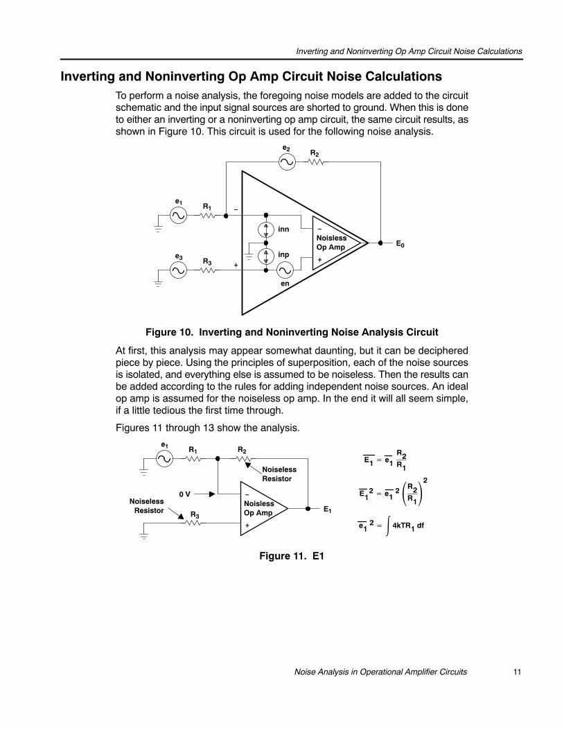
Inverting and Noninverting Op Amp Circuit Noise CalculationsTo perform a noise analysis, the foregoing noise models are added to the circuitschematic and the input signal sources are shorted to ground. When this is doneto either an inverting or a noninverting op amp circuit, the same circuit results, asshown in Figure 10. This circuit is used for the following noise analysis.

−NoislessOp Amp

+

−

+

en

inn

inp

e2 R2

e1 R1

e3 R3

E0

Figure 10. Inverting and Noninverting Noise Analysis Circuit

At first, this analysis may appear somewhat daunting, but it can be decipheredpiece by piece. Using the principles of superposition, each of the noise sourcesis isolated, and everything else is assumed to be noiseless. Then the results canbe added according to the rules for adding independent noise sources. An idealop amp is assumed for the noiseless op amp. In the end it will all seem simple,if a little tedious the first time through.

Figures 11 through 13 show the analysis.

E1 e1R2R1

E 21 e1

2 R2R12

e12 4kTR1 df

−NoislessOp Amp

+

R2e1 R1

R3E1

NoiselessResistor

0 VNoiseless

Resistor

Figure 11. E1


12 SLVA043A

E2 e2

e22 4kTR2 df

E 22 e2

2−NoislessOp Amp

+

R2e2R1

R3E2

0 VNoiseless

Resistor

NoiselessResistor

Figure 12. E2

E3 e3 R1 R2R1

E 22 e2

2 R1 R2R12

e32 4kTR3 df

−NoislessOp Amp

+

R2

e3

R1

R3E3

NoiselessResistor

NoiselessResistor

Figure 13. E3

Combining to arrive at the solution for the circuit’s output rms noise voltage,ERrms , due to the thermal noise of the resistors in the circuit:

ERrms E 21 E 2

2 E 23

ERrms

4kTR1R2R12

4kTR2 4kTR3R1 R2R12

df

ERrms

4kTR2R1 R2R1 4kTR3R1 R2

R12

df

If it is desired to know the resistor noise referenced to the input, EiRrms , the outputnoise is divided by the noise gain, An, of the circuit:

An R1 R2R1

(12)

(13)



E 2iRrms ERrms

An2

4kTR2 R1R2

R1 4kTR3R1R2

R12

df

R1R2R12

4kT R1R2R1 R2

R3df

Normally R3 is chosen to be equal to the parallel combination of R1 and R2 tominimize offset voltages due to input bias current. If this is done, the equationsimplifies to:

EiRrms 8kTR3 df When R3 R1R2R1 R2

Now consider the noise sources associated with the op amp itself. The analysisproceeds as before as shown in Figures 14 through 16.

En2 (en) R1 R2

R12

df

−NoislessOp Amp

+

en

R2R1

R3

Ep

NoiselessResistors

NoiselessResistor

Figure 14. Ep

Enp2 inpR3

R1 R2R12

df

−NoislessOp Amp

+

R2R1

R3

Enp

NoiselessResistors

NoiselessResistor inp

Figure 15. Enp

(14)

(15)


14 SLVA043A

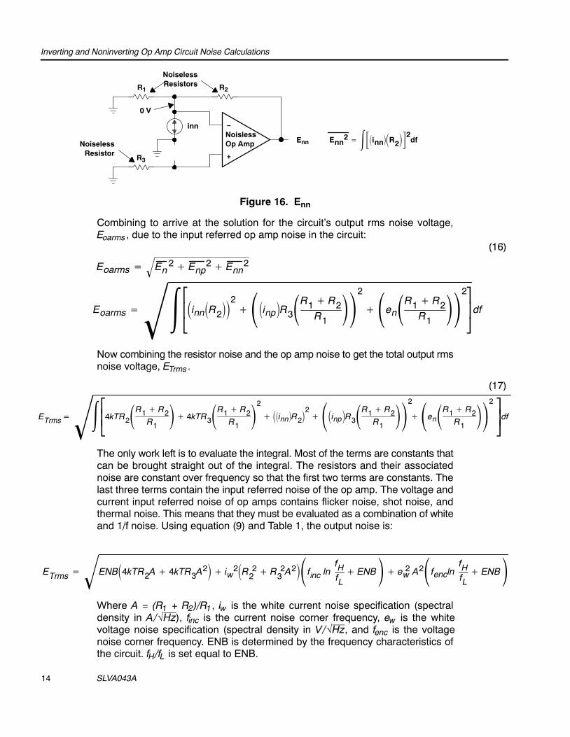
Enn2 innR2

2df

−NoislessOp Amp

+

R2R1

R3

Enn

NoiselessResistors

NoiselessResistor

inn

0 V

Figure 16. Enn

Combining to arrive at the solution for the circuit’s output rms noise voltage,Eoarms , due to the input referred op amp noise in the circuit:

Eoarms E 2n E 2

np E 2nn

Eoarms innR2

2 inpR3R1 R2R12

enR1 R2R12

df

Now combining the resistor noise and the op amp noise to get the total output rmsnoise voltage, ETrms .

ETrms


R12

innR22 inpR3R1 R2

R12

enR1 R2R12

dfThe only work left is to evaluate the integral. Most of the terms are constants thatcan be brought straight out of the integral. The resistors and their associatednoise are constant over frequency so that the first two terms are constants. Thelast three terms contain the input referred noise of the op amp. The voltage andcurrent input referred noise of op amps contains flicker noise, shot noise, andthermal noise. This means that they must be evaluated as a combination of whiteand 1/f noise. Using equation (9) and Table 1, the output noise is:

ETrms ENB4kTR2A 4kTR3A2 i 2w R 2

2 R 23 A2finc ln

fHfL

ENB e 2w A2fencln

fHfL

ENBWhere A = (R1 + R2)/R1, iw is the white current noise specification (spectraldensity in A/√Hz), finc is the current noise corner frequency, ew is the whitevoltage noise specification (spectral density in V/√Hz, and fenc is the voltagenoise corner frequency. ENB is determined by the frequency characteristics ofthe circuit. fH/fL is set equal to ENB.

(16)

(17)

Differential Op Amp Circuit Noise Calculations


In CMOS input op amps, noise currents are normally so low that the input noisevoltage dominates and the iw terms are not factored into the noise computation.Also, since bias current is very low, there is no need to use R3 for bias currentcompensation, and it, too, is removed from the circuit and the calculations. Withthese simplifications the formula above reduces to:

ETrms ENB 4kTR2 A e 2w A2fenc ln

fHfL

ENB CMOS input op amps


A noise analysis for a differential amplifier can be done in the same manner asthe previous example. Figure 17 shows the circuit used for the analysis.

−NoislessOp Amp

+

−

+

en

inn

inp

e2 R2

e1 R1

e3 R3

E0

R4

e4

Figure 17. Differenital Op Amp Circuit Noise Model

Figures 18 through 21 show the analysis.

E21 e2

1 R2R12−

NoiselessOp Amp

+

R2e1 R1

R3E1

0 V

R4

NoiselessResistors

NoiselessResistors

Figure 18. e1


16 SLVA043A

E 22 e 2

2

−

NoiselessOp Amp

+

R2e2R1

R3E2

0 V

R4

NoiselessResistors

NoiselessResistors

Figure 19. e2

E 23 e3

2 R4R3 R4

R1 R2R12−

+

R2

e3

R1

R3E3

R4

NoiselessOp Amp

Noiseless Resistors

NoiselessResistors

Figure 20. e3

E 24 e4

2 R3R3 R4

R1 R2R12−

NoiselessOp Amp

+

R2

e4

R1

R3E4

R4NoiselessResistors

NoiselessResistors

Figure 21. e4



Combining to arrive at the solution for the circuit’s output rms noise voltage,ERrms , due to the thermal noise in the resistors in the circuit:

ERrms E12 E22 E32 E42

ERrms4kTR1R2

R12 (4kTR2) 4kTR3 R4

R3 R42R1 R2

R124kTR4 R3

R3 R42R1 R2

R12df

ERrms 4kTR2R1

2 R2 R3 R4

R3 R42R1 R2

R12R4 R3

R3 R42R1 R2

R12df

Normally R1 = R3 and R2 = R4. Making this substitution reduces the above equation to:

ERrms 8kTR21 R2R1 df If R1 R3 and R2 R4

Now consider the noise sources associated with the op amp itself. The analysisproceeds as before as shown in Figures 22 through 24.

Enp2 inp R3R4R3 R4

R1 R2R1

2

df

−

NoiselessOp Amp

+

R2R1

R3

Enp

NoiselessResistors

NoiselessResistors

inp

Figure 22. inp

En2 (en)R1 R2R1

2

df

−

+

R2R1

R3

Ep

NoiselessResistors

NoiselessResistors

en

NoiselessOp Amp

Figure 23. en

(18)

(19)


18 SLVA043A

Enn 2 [(inn)(R2)]2df

−

+

R2R1

R3

Enn

NoiselessResistors

NoiselessResistors

inn

NoiselessOp Amp

Figure 24. inn

Combining to arrive at the solution for the circuit’s output rms noise voltage,Eoarms , due to the input referred op amp noise in the circuit:

Eoarms En 2 Enp 2 Enn 2

Eoarms ((inn) R2)2 (inp) R3R4R3 R4

R1 R2R1

2en R1 R2

R12

df

Normally R1 = R3, R2 = R4, and inn = inp = in. Making this substitution reducesthe above equation to:

Eoarms (2inR2)2 en R1 R2R1

2

df

R1 R3, R2 R4 and inn inp in

(20)

(21)



Now combine the resistor noise and the op amp noise to get the total output rmsnoise voltage, ETrms .

ETrms ((inn) R2)2 (inp) R3R4R3 R4

R1 R2R1

2

en R1 R2R1

24kTR1R2

R12

(4kTR2) 4kTR3 R4R3 R4

2R1 R2

R124kTR4 R3

R3 R42R1 R2

R12df

ETrms ((inn) R2)2 (inp) R3R4R3 R4

R1 R2R1

2

en R1 R2R1

2

4kT

R2R1

2 R2 R3 R4

R3 R42R1 R2

R12R4 R3

R3 R42R1 R2

R12

df

Substituting R1 = R3, R2 = R4, and inn = inp = in:

ETrms 2 (inR2)2 en R1 R2R1

2 8kTR2 R1 R2

R1df

R1 R3, R2 R4 and inn inp in

Evaluating the integral using these simplifications results in:

ETrms ENB 8kTR2A 2i 2w R 2

2 finc ln

fHfL

ENB e 2w A2 fenc ln

fHfL

ENBR1 R3, R2 R4 and inn inp in

Where A = (R1 + R2)/R1, iw is the white current noise specification (spectraldensity in A/√Hz), finc is the current noise corner frequency, ew is the white voltagenoise specification (spectral density in V/√Hz ), and fenc is the voltage noisecorner frequency. ENB is determined by the frequency characteristics of thecircuit. fH/fL is set equal to ENB.

(22)

(23)

(24)

Summary

20 SLVA043A

SummaryThe techniques presented here can be used to perform a noise analysis on anycircuit. Superposition was chosen for illustrative purposes, but the samesolutions can be derived by using other circuit analysis techniques.

Noise is a purely random signal; the instantaneous value and/or phase of thewaveform cannot be predicted at any time. The only information available forcircuit calculations is the average mean-square value of the signal. With multiplenoise sources in a circuit, the total root-mean-square (rms) noise signal thatresults is the square root of the sum of the average mean-square values of theindividual sources.

ETotalrms e21rms e2

2rms ...e2nrms

Because noise adds by the square, when there is an order of magnitude or moredifference in value, the lower value can be ignored with very little error. Forexample:

12 102 10.05

If the 1 is ignored, the error is 0.5%. With modern computational resources,evaluation of all the terms is trivial, but it is important to understand the principlesso that time will be spent reducing the 10 before working on the 1.

Noise is normally specified as a spectral density in rms volts or amps per rootHertz, V/√Hz or A/√Hz. To calculate the amplitude of the expected noise signal,the spectral density is integrated over the equivalent noise bandwidth (ENB) ofthe circuit.

Very often the peak-to-peak value of the noise is of interest. Once the total rmsnoise signal is calculated, the expected peak-to-peak value can be calculated.The instantaneous value will be equal to or less than 6 times the rms value 99.7%of the time.

References


References1. J. B. Johnson. Thermal Agitation of Electricity in Conductors. Physical

Review, July 1928, Vol. 32.

2. Aldert van der Ziel. Noise. Prentice-Hall, Inc., 1954.

3. H. Nyquist. Thermal Agitation of Electric Charge in Conductors. PhysicalReview, July 1928, Vol. 32.

4. Paul R. Gray and Robert G Meyer. Analysis and Design of Analog IntegratedCircuits. 2d ed., John Wiley & Sons, Inc., 1984.

5. Sergio Franco. Design with Operational Amplifiers and Analog IntegratedCircuits. McGraw-Hill, Inc., 1988.

6. David E. Johnson, Johnny R. Johnson, and John L. Hilburn. Electric CircuitAnalysis. Prentice-Hall, Inc., 1989.

Using Current Sources for Resistor Noise Analysis

A-1 Noise Analysis in Op Amp Circuits

Appendix A Using Current Sources for Resistor Noise AnalysisFigures A1 through A3 show analysis of the resistor noise in theinverting/noninverting op amp noise analysis circuit using current sources inparallel with the noiseless resistors.

E1 i1 R1R2R1

i1R2

E 21 i1R2

2

i12 4kT

R1df

−

NoiselessOp Amp

+

R2R1

R3

0 V

i1

NoiselessResistor

NoiselessResistor

Figure A−1. E1

E2 i2 R2

E 22 i2R2

2

i22 4kT

R2df

−

+

R2R1

R3

0 V

i2

NoiselessResistors

NoiselessOp Amp

Figure A−2. E2

E3 i3 R3 R1 R2R1

E 23 i3 R3 R1 R2

R12

i32 4kT

R3df

−

+

R2R1

R3

i3

NoiselessOp Amp

Figure A−3. E3

Using Current Sources for Resistor Noise Analysis

A-2 SLVA043A

Combining the independent noise signals:

ERrms E 21 E 2

2 E 23

ERrms

4kTR1

R22 4kT

R2R2

2 4kTR3

R23R1 R2

R12

df

ERrms


R12

df

The resulting equation is the same as equation (12) presented earlier.

(A−1)

IMPORTANT NOTICE

Texas Instruments Incorporated and its subsidiaries (TI) reserve the right to make corrections, modifications, enhancements,improvements, and other changes to its products and services at any time and to discontinue any product or service without notice.Customers should obtain the latest relevant information before placing orders and should verify that such information is current andcomplete. All products are sold subject to TI’s terms and conditions of sale supplied at the time of order acknowledgment.

TI warrants performance of its hardware products to the specifications applicable at the time of sale in accordance with TI’sstandard warranty. Testing and other quality control techniques are used to the extent TI deems necessary to support thiswarranty. Except where mandated by government requirements, testing of all parameters of each product is not necessarilyperformed.

TI assumes no liability for applications assistance or customer product design. Customers are responsible for their products andapplications using TI components. To minimize the risks associated with customer products and applications, customers shouldprovide adequate design and operating safeguards.

TI does not warrant or represent that any license, either express or implied, is granted under any TI patent right, copyright, maskwork right, or other TI intellectual property right relating to any combination, machine, or process in which TI products or servicesare used. Information published by TI regarding third-party products or services does not constitute a license from TI to use suchproducts or services or a warranty or endorsement thereof. Use of such information may require a license from a third party underthe patents or other intellectual property of the third party, or a license from TI under the patents or other intellectual property of TI.

Reproduction of information in TI data books or data sheets is permissible only if reproduction is without alteration and isaccompanied by all associated warranties, conditions, limitations, and notices. Reproduction of this information with alteration is anunfair and deceptive business practice. TI is not responsible or liable for such altered documentation.

Resale of TI products or services with statements different from or beyond the parameters stated by TI for that product or servicevoids all express and any implied warranties for the associated TI product or service and is an unfair and deceptive businesspractice. TI is not responsible or liable for any such statements.

TI products are not authorized for use in safety-critical applications (such as life support) where a failure of the TI product wouldreasonably be expected to cause severe personal injury or death, unless officers of the parties have executed an agreementspecifically governing such use. Buyers represent that they have all necessary expertise in the safety and regulatory ramificationsof their applications, and acknowledge and agree that they are solely responsible for all legal, regulatory and safety-relatedrequirements concerning their products and any use of TI products in such safety-critical applications, notwithstanding anyapplications-related information or support that may be provided by TI. Further, Buyers must fully indemnify TI and itsrepresentatives against any damages arising out of the use of TI products in such safety-critical applications.

TI products are neither designed nor intended for use in military/aerospace applications or environments unless the TI products arespecifically designated by TI as military-grade or "enhanced plastic." Only products designated by TI as military-grade meet militaryspecifications. Buyers acknowledge and agree that any such use of TI products which TI has not designated as military-grade issolely at the Buyer's risk, and that they are solely responsible for compliance with all legal and regulatory requirements inconnection with such use.

TI products are neither designed nor intended for use in automotive applications or environments unless the specific TI productsare designated by TI as compliant with ISO/TS 16949 requirements. Buyers acknowledge and agree that, if they use anynon-designated products in automotive applications, TI will not be responsible for any failure to meet such requirements.

Following are URLs where you can obtain information on other Texas Instruments products and application solutions:

Products Applications

Amplifiers amplifier.ti.com Audio www.ti.com/audio

Data Converters dataconverter.ti.com Automotive www.ti.com/automotive

DSP dsp.ti.com Broadband www.ti.com/broadband

Interface interface.ti.com Digital Control www.ti.com/digitalcontrol

Logic logic.ti.com Military www.ti.com/military

Power Mgmt power.ti.com Optical Networking www.ti.com/opticalnetwork

Microcontrollers microcontroller.ti.com Security www.ti.com/security

RFID www.ti-rfid.com Telephony www.ti.com/telephony

Low Power www.ti.com/lpw Video & Imaging www.ti.com/videoWireless

Wireless www.ti.com/wireless

Mailing Address: Texas Instruments, Post Office Box 655303, Dallas, Texas 75265Copyright © 2007, Texas Instruments Incorporated

http://amplifier.ti.com

http://www.ti.com/audio

http://dataconverter.ti.com

http://www.ti.com/automotive

http://dsp.ti.com

http://www.ti.com/broadband

http://interface.ti.com

http://www.ti.com/digitalcontrol

http://logic.ti.com

http://www.ti.com/military

http://power.ti.com

http://www.ti.com/opticalnetwork

http://microcontroller.ti.com

http://www.ti.com/security

http://www.ti-rfid.com

http://www.ti.com/telephony

http://www.ti.com/lpw

http://www.ti.com/video

http://www.ti.com/wireless

Noise Analysis In Operational Amplifier Circuits - Texas Instruments

Documents

Transcript of Noise Analysis In Operational Amplifier Circuits - Texas Instruments