NOAA Technical Memorandum ERL PMEL-54

METLIB-II - A PROGRAM LIBRARY FOR CALCULATING AND PLOTTING

ATMOSPHERIC AND OCEANIC FIELDS

S. A. MacklinR. L. BrownJ. GrayR. W. Lindsay

Pacific Marine Environmental LaboratorySeattle, WashingtonApril 1984

UNITED STATESDEPARTMENT OF COMMERCE

Malcolm Baldrlg..Secntary

NATIONAL OCEANIC AND.ATMOSPHERIC ADMINISTRATION

John V. Byrne,Administrator

Environmental Researchlaboratories

Vernon E. DerrDirector

NOTICE

Mention of a commercial company or product does not constitutean endorsement by NOAA Environmental Research Laboratories.Use for publicity or advertising purposes of information fromthis publication concerning proprietary products or the testsof such products is not authorized.

i i

CONTENTS

PageAbstract 11. INTRODUCTION 22. COMPUTING WITH MElLIB-II 33. DATA SOURCES 74. DATA MANAGEMENT 85. MAIN PROGRAMS 13

5.1 UNPACK (Used to Extract Subsets from large Temporal orGeographic Data Sets Such as NCAR) 13

5.2 DECKS (Creates a Standard Format File from Digitized Fields) 165.3 WINDS (Calculations of Winds) 185.4 PNTWIND (Time Series of Winds) 255.5 TRKWIND (Time Series of Winds Following a Track line) 275.6 METlOOK (Prints Records from METlIB Files) 295.7 FORMAT (Creates Formatted Files from METlIB Files) 305.8 PlOTGRD (Plots METlIB Fields) 325.9 DRAWMAP (Draws Grid with Continental Outlines) 40

6. SUBROUTINE DOCUMENTATION 416.1 Introduction 416.2 list of Subroutines 426.3 Interpolation (NTERP) 436.4 location on SUbgrid (IJ2ll,ll2IJ) 436.5 Speed and Direction (SD2UV,UV2SD) 446.6 Thermal Wind (THRMWND) 456.7 Grid Initialization (GRIDSET) 456.8 Geostrophic Wind (GEOWIND,EDGE) 456.9 Gradient Wind (GRADWND) 466.10 Wind Models (MODEl2, 4, 6, 8, BROWN, CARDON, etc.) 46

7. ACKNOWLEDGEMENTS 498. REFERENCES 50APPENDIX: DIGITIZING DATA FROM CHARTS - AN EXAMPLE 52

iii

METlIB-II - A PROGRAM lIBRARY FOR CALCULATING AND PLOTTINGATMOSPHERIC AND OCEANIC FIELDS

S. A. MacklinR. l. Brown

J. GrayPacific Marine Environmental laboratory

Seattle. Washington

R. W. lindsayUniversity of Washington

Seattle. Washington

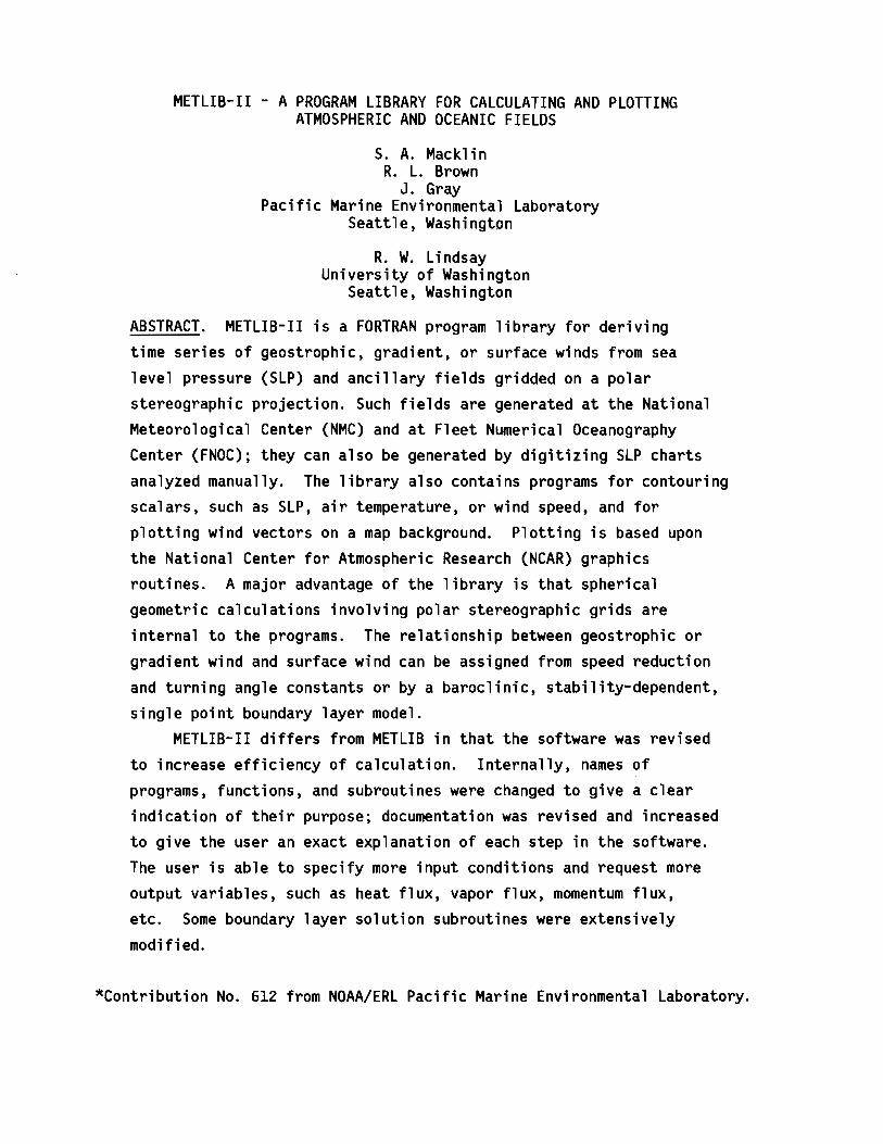
ABSTRACT. METlIB-II is a FORTRAN program library for derivingtime series of geostrophic. gradient. or surface winds from sea

level pressure (SlP) and ancillary fields gridded on a polarstereographic projection. Such fields are generated at the NationalMeteorological Center (NMC) and at Fleet Numerical OceanographyCenter (FNOC); they can also be generated by digitizing SlP charts

analyzed manually. The library also contains programs for contouringscalars. such as SlP. air temperature. or wind speed. and forplotting wind vectors on a map background. Plotting is based uponthe National Center for Atmospheric Research (NCAR) graphicsroutines. A major advantage of the library is that sphericalgeometric calculations involving polar stereographic grids areinternal to the programs. The relationship between geostrophic or

gradient wind and surface wind can be assigned from speed reductionand turning angle constants or by a baroclinic. stability-dependent.single point boundary layer model.

METlIB-II differs from METlIB in that the software was revised

to increase efficiency of calculation. Internally. names ofprograms. functions. and subroutines were changed to give a clearindication of their purpose; documentation was revised and increasedto give the user an exact explanation of each step in the software.The user is able to specify more input conditions and request more

output variables. such as heat flux. vapor flux. momentum flux.etc. Some boundary layer solution subroutines were extensivelymodified.

*Contribution No. 612 from NOAA/ERl Pacific Marine Environmental laboratory.

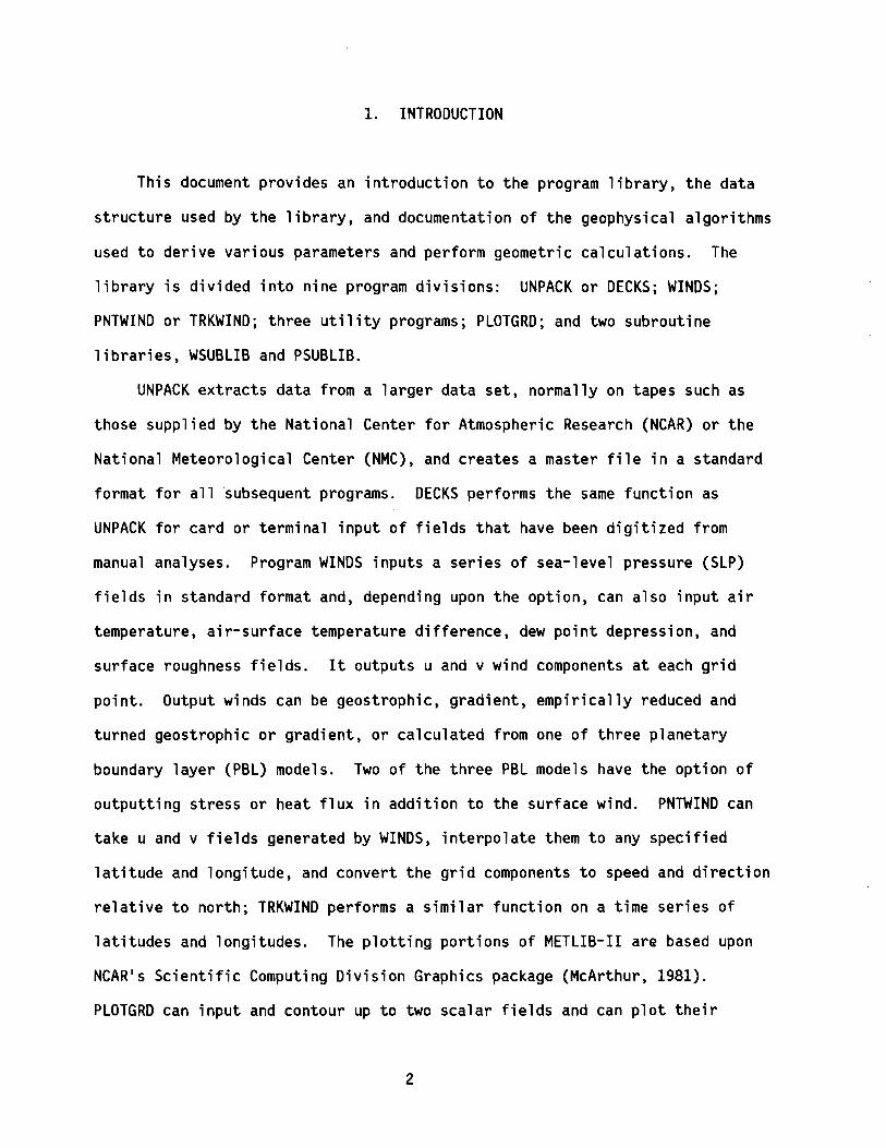
1. INTRODUCTION

This document provides an introduction to the program library, the data

structure used by the library, and documentation of the geophysical algorithms

used to derive various parameters and perform geometric calculations. The

library is divided into nine program divisions: UNPACK or DECKS; WINDS;

PNTWIND or TRKWIND; three utility programs; PlOTGRD; and two subroutine

libraries, WSUBlIB and PSUBlIB.

UNPACK extracts data from a larger data set, normally on tapes such as

those supplied by the National Center for Atmospheric Research (NCAR) or the

National Meteorological Center (NMC) , and creates a master file in a standard

format for all sUbsequent programs. DeCKS performs the same function as

UNPACK for card or terminal input of fields that have been digitized from

manual analyses. Program WINDS inputs a series of sea-level pressure (SlP)

fields in standard format and, depending upon the option, can also input air

temperature, air-surface temperature difference, dew point depression, and

surface roughness fields. It outputs u and v wind components at each grid

point. Output winds can be geostrophic, gradient, empirically reduced and

turned geostrophic or gradient, or calculated from one of three planetary

boundary layer (PBl) models. Two of the three PBl models have the option of

outputting stress or heat flux in addition to the surface wind. PNTWIND can

take u and v fields generated by WINDS, interpolate them to any specified

latitude and longitude, and convert the grid components to speed and direction

relative to north; TRKWIND performs a similar function on a time series of

latitudes and longitudes. The plotting portions of METlIB-II are based upon

NCAR's Scientific Computing Division Graphics package (McArthur, 1981).

PlOTGRD can input and contour up to two scalar fields and can plot their

2

difference. It can draw arrow plots of a vector field or the difference of

two vector fields t and can plot a vector field with contours of a scalar t

including contours of the magnitude (isotachs) of the vector field itself or

the difference in magnitude of two vector fields. All routines are intended

to be machine-independent FORTRAN 66 programs.

For use at the Pacific Marine Environmental laboratory (PMEl) or other

locations with access to the Environmental Research laboratories· (ERl) CDC

Cyber 750 computer in Boulder t Colorado t SUBMIT files are shown for each of

the main programs for METlIB-II. These SUBMIT files all have filenames

beginning with the letter J and are specific to the ~OS 2.0 operating system

in use at the time of pUblication.

METlIB-II is a direct outgrowth of METlIB - A PROGRAM lIBRARY FOR

CALCULATING AND PLOTTING MARINE BOUNDARY lAYER WIND FIELDS by Overland t et

al. (1980). METlIB-II offers a more liberal choice of input and output

fields t computes more accurately and efficientlYt and provides three levels

of output documentation. InternallYt subroutine and program names have been

changed to better reflect their purpose t and documentation has been added at

appropriate steps. The surface wind model 6 has been revised extensively.

Complete listings of programs and subroutines are available from the authors.

2. COMPUTING WITH METlIB-II

METlIB-II is a library of FORTRAN programs that are used for batch

processing; this means that jobs are submitted to the computer for processing

independent of any other computer execution a user may be undertaking t such

as a terminal session. We proceed in this manner because METlIB programs

3

often require the mounting of tapes or disk packs, and require lengthy execution

times because of the vast amount of data that is processed. Batch processing

allows the user to continue interacting with other computer work at the

terminal without waiting for the METLIB job to terminate.

Most METLIB jobs have four components:

1. input data files,

2. Fortran program and subroutine library,

3. output data files, and

4. job control language (SUBMIT files) to instruct the computer

on how to assign, link and execute the above three items.

Input data files may be in the form of raw data tapes or card decks, but

generally they will be gridded data created with a format compatible with the

programs presently residing in METLIB. Output data, too, are generally

METLIB format files. The Fortran programs and their required input and

output data assignments are discussed in section 5 of this document. We have

tried to use standard Fortran 66 statements throughout the library, however,

the UNPACK routine, for reading raw data tapes, uses system-defined, word-size­

dependent utilities that will depend on the conditions set by the computer

which created the tapes. Job control statements in the SUBMIT files are

dictated by the operating system employed by each particular computer.

Examples of job control language for the Network Operating System (NOS) in

place on the NOAA Cyber 750 computer in Boulder, Colorado, are presented for

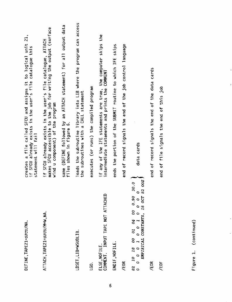
each main program. Figure 1 gives a brief explanation of each of the job

control statements in the SUBMIT file JWINDS. All the ATTACH statements

assign a logical unit number (for example, TAPE10) to each input and output

data file. The many available program options are controlled by the data

card variables set by the user. Many of the data cards are in free

4

<.11

/JOB

JWIN

DS.

lie /REA

D,U

SERI

D

/NOS

EQ

GET

,WIN

DS.

FTN

,I=W

IND

S,R=

O,L

=O,P

MD

.

RETU

RN,W

IND

S.

GET

,WSU

BLIB

/UN

=MET

LIB.

ATT

ACH

,TA

PE10

=SLP

/NA

.

IFE

,FIL

E(T

APE

10,B

OI)

,NO

FIL

E.

tell

sth

eco

mpu

ter

toex

pect

ase

quen

ceof

job

cont

rol

stat

emen

ts

nam

eof

the

SUBM

ITfi

le

ast

ar

inco

lum

n1

foll

owed

bya

spac

ein

dic

ates

aco

mm

ent

card

read

sth

eu

ser'

sna

me,

char

ge,

pro

ject

num

ber,

and

rout

ing

info

rmat

ion

(fo

rp

rin

ted

outp

ut)

from

afi

lecr

eate

dby

the

user

call

edUS

ERID

(res

ides

inth

eu

ser'

spe

rman

ent

file

spac

e)

allo

ws

data

entr

yto

begi

nin

colu

mn

1

find

sth

esp

ecif

ied

mai

npr

ogra

m(e

x.W

INDS

)in

the

use

r's

perm

anen

tfi

lesp

ace

and

mak

esit

acce

ssib

leto

the

job

sequ

ence

com

pile

sth

esp

ecif

ied

For

tran

prog

ram

;R

,Lan

dPM

Dar

eou

tput

spec

ific

atio

ns

rele

ases

the

unco

mpi

led

copy

ofW

INDS

find

sth

esu

brou

tine

lib

rary

WSU

BLIB

inac

coun

tM

ETLI

B

find

sth

ein

put

data

file

(SL

P),

assi

gns

itto

logi

cal

un

it10

,an

dm

akes

itac

cess

ible

toth

epr

ogra

m

ifTA

PE10

isno

tat

tach

edor

rew

ound

then

skip

toth

eEL

SE,N

OFI

LE.

stat

emen

t

sam

e(A

TTAC

Hfo

llow

edby

anIF

Est

atem

ent)

for

all

inpu

tda

tafi

les

show

nin

figu

re6.

Fig

ure

1.An

anno

tate

dve

rsio

nof

the

SUBM

ITfi

leJW

INDS

illu

stra

tes

the

mea

ning

ofth

eNO

S2.

0jo

bco

ntro

lla

ngua

geus

edin

MET

LIB

-II.

The

wor

dsan

dnu

mbe

rsin

itali

cs

are

set

byth

eus

eran

dar

eex

plai

ned

inse

ctio

ns

4an

d5.

0'\

DEF

INE.

TAPE

21=S

FCV

/NA

.

ATT

ACH

.TA

PE21

=SFC

VIM

=W.N

A.

LDSE

T.LI

B=W

SUBL

IB.

LGO.

ELSE

.NO

FILE

.CO

MM

ENT.

INPU

TTA

PENO

TAT

TACH

ED

ENDI

F•N

OFIL

E.

IEO

R

crea

tes

afi

leca

lled

SFCU

and

assi

gn

sit

tolo

gic

alu

nit

21.

ifSF

CUal

read

yex

ists

inth

eu

ser'

sfi

leca

talo

gue

this

stat

emen

tw

ill

fail

ifSF

CUal

read

yex

ists

inth

eu

ser'

sfi

leca

talo

gu

e.AT

TACH

mak

esSF

CUac

cess

ible

toth

ejo

bfo

rw

riti

ng

the

outp

ut(s

urf

ace

win

du

com

pone

nt)

of

the

prog

ram

sam

e(D

EFIN

Efo

llow

edby

anAT

TACH

stat

emen

t)fo

ral

lou

tput

dat

afi

les

show

nin

fig

ure

6.

load

sth

esu

brou

tine

lib

rary

into

LIB

whe

reth

epr

ogra

mca

nac

cess

the

subr

outi

nes

wit

ha

CALL

stat

emen

t

exec

utes

(or

runs

)th

eco

mpi

led

prog

ram

ifan

yo

fth

eIF

Est

atem

ents

are

tru

e.th

eco

mpu

ter

skip

sth

ein

term

edia

test

atem

ents

and

pri

nts

the

COM

MEN

T

ends

the

po

rtio

no

fth

eSU

BMIT

rou

tin

eto

whi

chIF

Esk

ips

end

of

reco

rdsi

gn

als

the

end

of

the

job

cont

rol

lang

uage

82

10

18

00

010

40

00

.90

30

.0}

o0

00

10

01

00

00

EM

PIR

ICA

LC

ON

STAN

TS,

18

OCT

82

OO

Zd

ata

card

s

IEO

Ren

do

fre

cord

sig

nal

sth

een

do

fth

ed

ata

card

s

IEO

Fen

do

ffi

lesi

gn

als

the

end

of

this

job

Fig

ure

1.

(con

tinu

ed)

field format meaning that the numbers must only be in the correct order and

separated by commas or spaces.

METLIB is generally used in the following sequence: first, raw pressure

(and sometimes, temperature, humidity, etc.) fields are transformed into

METLIB files using DECKS (card decks) or UNPACK (tape); next, these METLIB

files are submitted to WINDS to generate u and v wind components; maps of the

wind, temperature, and pressure fields are then created by PLOTGRD; and

finally, time series of winds are produced by PNTWIND or TRKWIND.

All the METLIB main programs, SUBMIT files, and subroutine libraries

reside in a separate account on the ERL CDC computer in Boulder, CO. In

order to keep the master account files unchanged, we ask that users with

access to the ERL CDC make copies of the main programs and SUBMIT files they

need. The appropriate changes (dimensions, file names, titles) can then be

made and the programs can be submitted from the users' accounts.

3. DATA SOURCES

NMC currently produces SLP and surface air temperature (SAT) analyses at

0000 and 1200 GMT on one of two polar stereographic meshes: the PE 65 x 65

point grid, with a spacing of 381 km at GOoN, covering the northern hemisphere;

and the LFM 53 x 57 point grid, a fine-mesh grid with a spacing of 190.5 km

at GOoN, covering North America and the adjacent waters (Figures 2 and 3).

PE and LFM are historical names standing for IIfrimitive £quation ll and lI.!:imited

Area fine-Mesh ~odel". The PE data are archived at NCAR (Jenne, 1975) and at

the National Climatic Center (NCC). At present the LFM data are not routinely

archived for general distribution. Pressure fields are also produced by the

7

Fleet Numerical Oceanography Center (FNOC) at 0000, 0600, 1200, and 1800 GMT

on a 63 x 63 point grid with the same scale and orientation as the PE grid.

All grids are uniformly spaced upon a polar stereographic map projection,

which preserves angles (Figures 2 and 3).

Internal north-pole coordinates are (33,33) for the PE grid and (27,49)

for the LFM. The FNOC pressure fields have pole coordinates of (32,32). For

PE data prior to 1976 the NMC "octagon" was used. The number of grid points

was 47 x 51, the pole location was (24,26), and the data were stored in a

one-dimensional array. This is the format used by NCAR to store much of

their NMC PE data.

Over the ocean, SLP and SAT values for operational forecast models are

obtained from ocean-station vessel, buoy and ship observations analysed by a

variety of objective analysis techniques (Cressman, 1959; Flattery, 1970;

Holl and Mendenhall, 1971). For many research purposes it is necessary to

reanalyze the SLP charts making use of reports that were not included in the

NMC analysis. To this end, the reanalysis is done on a standard polar

stereographic projection and digitized at a uniform spacing compatible with

either the PE or LFM grids. The digitizing process is explained in the

Appendix.

4. DATA MANAGEMENT

All master data files created by UNPACK or DECKS are in a standard

format for subsequent processing. Master data sets are arranged

chronologically and separated by type (e.g., SLP or wind speed) and geo­

graphical region (e.g., the Gulf of Alaska). Thus, one file might have a

8

'., , , ,

, ,

,, ,.-'

" .." "

",",,

,",

" , ,."

I, " 'M "

, , ,. . '." ,. . , ..

",

"

,.

"", "

...' "'.

"

. '

, '

, '

'. '

..

, ..

, .'.,

. .., ....,,

. ,." , .' .' , "

l ""'•. ,. .;C ,', i . 'II-M1HH.........:.J.-+-++-f.:~¥=f-ftl-l-H~'4-+-=!s!f-+-r~r.f.t+:;iIj ...~I-_ ., f.l,:+-"J,~.:t+"'!If+.p""'t-f-.-.HI-f:IH:ot~:tf-+++++-Hl-HI+-lH

, "" ..~ J.

..... ',,:' ,

..... "

~ .. ',. ,. ", "

.. ,'.

'...

.', ,

- ,'j: .

'i .: ~:. ,:

'. ~ _.. ..:,

...•... ,~

"

,, ," ,

.' .

,'. ..,. ": " .~. "

.. ,.," '. ', . "

" .'.

. .I "

,. "

'.

..-, /

Figure 2. Some PE data are stored in a 65 x 65 point grid. FNOC uses a63 x 63 grid with the same mesh point locations and center point.Prior to 1976, PE data were archived in the 47 x 51 point NMC"octagon". These grids have internal north-pole coordinates (33,33),(32,32), and (24,26), respectively, and are IGRID options 1, 4, and3 in programs UNPACK and DECKS.

9

"'."

... ......-

- L_

\. " .

1"\

\ I~ Ll..1';" \

, " • IJ

.. _..... ~ .... _.....

';c

~ 'cf -. -,

1\."' ..... "

Il~ ' ..

"

.~

I""

........ ,

. " ,.IT"

. "

,10 ... ......

]'

/, ,, '. '

'.r--·"-1!ooI.

. , ......

'1:::::(," "

. ',~',

',,:)' ,':,,: .'''''r-. ".' . ::., {":: ':\ ..' .', ' .. '1\

: '.I.}..•:~~'... " .. ,~""'". "1.;. i\ ~:r.,;;n ,...,. f~ "

..

" )' '~. .~

, , ., , ." ~~ ........ ' "

" .

"

-.

"

-- ... 1

.'

- -- _. ~

,'f~

"

• '10"'- _ ,....

"

I., ."

--~ ,

""

1'\

"

J •

-~ -- - 1;1- 11- -__

_ ._ .- - Kf .- -- -

L.,

.'

.....~ .....

.,,.

"

""

"

""

"

....~ ...

; '. '. '\.

\ ,"..: .:.-...."

" ', "

..,....,,,

I) .I\.. .'

\- ...-• '. ,~:. "rr... - ..~ _

" I.... .::...... t\. l" oJ

" '. , . l-: ~ ....~ ,.., .......

.... '. :.:. '.

,...

.':' .'

1\1

,I\. "

.., ."

"

"

., ,

"

,,

"

..

.. " .ti . .;.... .. '.I-HH-.."',o...t-+..>+--,,~,HH-rt-+-+-++tt-+-"~ __ _ ~.;_ .. - : " ". ;: ", ..I-Hf-,,*"+-+-+-j-.:J~, ~.,:oF-+-+-+-HiI'-f-f~ . r,1l.'T;t---hF..:.:l.F..::1.~:.:F.f:-.t-HH.~.,".-.. t.:"':::t:,:'l1:~j.-.,~:H.".+-#'".1l.'Y"..--I:-..f-+-t---f--HH,-+-1

.'

...,

....

....

..

"

..

"

.."'" I\.

.. , .'

\. .' ... : " "

" ,.,.. :.- ' L..o.

, :.

: -< " ~~

;.; : ".

' , " , .'.' ,.... •... I~

. .. ' '.: ",: ,,<:; :"I:f

............ , ~

'.' ". ~

,.' ..

, ., :

.:

· .· .

·;·:

:1'\" .

.. ...:.......: ....

.........

l\1\

'- - " ~- -__ LI --1 -- --rri 1.1

I\.

If

J '" f'

'i-4 , i

r .

'f "

"

"

.."

....

"

....

"

""

"

"

" '.

Figure 3., LFM data are stored in the NMC 53 x 57 point grid with north-polecoordinates (27,49). This grid is IGRID option 2 in programsUNPACK and DECKS.

10

I-year time series of daily observed SLP's in a 10 x 10 grid for the Gulf of

Mexico; another file might consist of model-generated t u-component winds for

the same period t etc.

All records are generated by FORTRAN unformatted write statements and

are stored in an unpacked form. Every METLIB data file is identified by a

header record. This header is the first card in the data file and consists

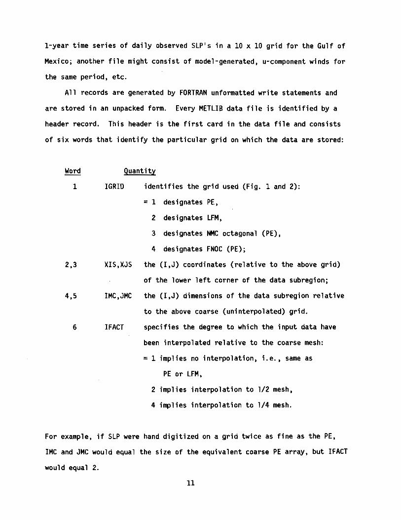
of six words that identify the particular grid on which the data are stored:

Word Quantity

1 IGRID identifies the grid used (Fig. 1 and 2):

=1 designates PEt

2 designates LFM,

3 designates NMC octagonal (PE),

4 designates FNOC (PE);

2,3 XIS,XJS the (I,J) coordinates (relative to the above grid)

of the lower left corner of the data subregion;

4,5 IMC,JMC the (I,J) dimensions of the data subregion relative

to the above coarse (uninterpolated) grid.

6 IFACT specifies the degree to which the input data have

been interpolated relative to the coarse mesh:

= 1 implies no interpolation, i.e., same as

PE or LFM,

2 implies interpolation to 1/2 mesh,

4 implies interpolation to 1/4 mesh.

For example, if SLP were hand digitized on a grid twice as fine as the PE,

IMC and JMC would equal the size of the equivalent coarse PE array, but IFACT

would equal 2.

11

The header is followed by as many data records as necessary. Each

record consists of a card containing seven identification words followed by

the data. The identification words specify the date and data characteristics

as follows:

Word

1

2

3

4

5

6

IYEAR

MONTH

IDAY

IHOUR

ITYPE

lOBS

Quantity

"68" means 1968,

"11" means November,

"03" means the third day of the month,

"12" means 12 GMT,

data type coded as in NMC office note 84 (1973):

= 8 implies pressure in mb,

16 implies air temperature in °C or oK,

17 implies dew point temperature (same units as

air temperature),

18 implies dew point depression in °C or oK,

30 implies air-surface temperature difference in

°C or oK,

88 implies relative humidity as a fraction of 1 (0-1),

384 implies surface temperature (in same units as

air temperature);

gives the type of forecast:

= 0 designates observed data,

12 designates 12-hr forecast data,

24 designates 24-hr forecast data, etc.,

910 designates climate type 1.0,

920 designates climate type 2.0, etc.;

12

7 IFLAG flags missing data:

= 0 means data are complete~

1 means data are missing.

Following these identification words~ the data array is written in words 8~

9~ 10~ etc. Missing data are given the value 9999. Two-dimensional arrays~

A(I~J)~ are structured so that I and J increase in the same direction as I

and J of the PE or LFM grids~ with A(l~l) at the lower left corner of the

subregion and the arrays reading ((A(I~J)~ 1=1~ IMC)~ J=l~ JMC).

5. MAIN PROGRAMS

5.1 UNPACK (Used to Extract Subsets from Large

Temporal or Geographic Data Sets such as NCAR)

UNPACK performs four tasks. It unpacks the data~ if necessary; extracts

the appropriate time series~ subregion~ data type~ and forecast type as

specified; interpolates the data to a finer (1/0FACT) mesh by biquadratic

interpolation; and organizes the data set into the standard format for use by

subsequent METLIB analysis routines. Since the raw data tapes come in

different formats~ UNPACK contains separate subroutines for each grid used

(at publication time~ subroutines exist only for the NMC octagonal and FNOC

grids). The user specifies the start and stop time of the file to be generated~

the grid to which the source data correspond~ the lower-left-corner coordinates

and dimensions of the region to be analyzed~ the data type~ the forecast

types~ the desired degree of interpolation~ and the number of hours between

map times on a single input data card with format (1713) as follows:

13

IYSTRT.

IMSTRT.

IDSTRT.

IHSTRT.

IYSTOP.

IMSTOP.

IDSTOP.

IHSTOP.

IGRID .

the year of the first desired datum (e.g. 71 for 1971),

the month (e.g. 03 for March),

the day,

the hour,

the year of the last desired datum,

the month,

the day,

the hour,

the grid used:

= 1 for PE (65 x 65),

= 2 for lFM (53 x 57),

= 3 for NMC octagonal (47 x 51),

=4 for FNOC PE (63 x 63);

ILl,JLL ... the lower left (I,J) coordinates measured on the

source grid of the desired geographical region;

IMC,JMC ... the number of (source) grid points to be taken in

the I and J directions to cover the desired geographical

region: the point (ILL,Jll) is counted as the first

point;

ITYPE .... METlIB data type codes as in NMC office note 84:

= 8 for pressure in millibars,

= 16 for air temperature in degrees Centigrade or Kelvin,

etc. (as listed in section 4, page 12);

IFCST . . . . the forecast type:

= 0 for observed data,

= 12 for 12-hr forecast data, etc.;

OFACT .... the degree of interpolation for output fields:

14

= 1 no interpolation

= 2 interpolate to 1/2 mesh

= 4 interpolate to 1/4 mesh;

MINOT . . . . the number of hours between map times.

The file generated by UNPACK is in standard format with a file header and a

time series of data records.

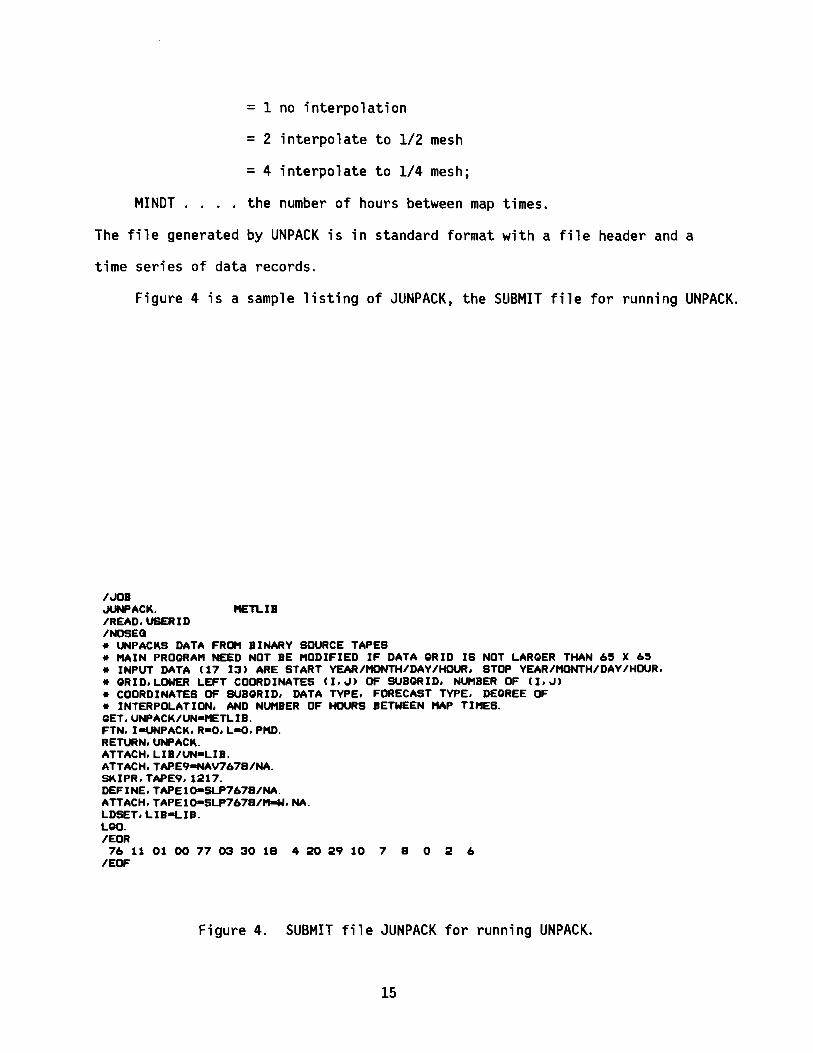
Figure 4 is a sample listing of JUNPACK. the SUBMIT file for running UNPACK.

I.JOB.JUNPACK. t£TLIBIREAD,USERIDINOSEQ* UNPACKS DATA FROM BINARV SOURCE TAPES* MAIN PROgRAM NEED NOT BE MODIFIED IF DATA gRID IS NOT LARgER THAN 6' X 6'* INPUT DATA (17 13) ARE START VEAR/MONTH/DAV/HOUR, STOP VEAR/MONTH/DAV/HOUR,* gRID, LOWER LEFT COORDINATES (I,.J) OF SUBQRID. NUMBER OF (I,.J)* COORDINATES OF SUBgRID. DATA TVPE. FORECAST TVPE. DEQREE OF* INTERPOLATION. AND NUMBER OF HOURS BETWEEN HAP TIMES.QET.UNPACK/UN-METLIB.FTN.I-UNPACK.R-O.L-O.PKD.RETURN. UNPACK.ATTACH.LIB/UN-LIB.ATTACH.TAPE9-NAV7678/NA.SKIPR.TAPE9.1217.DEFINE.TAPE10-SLP7678/NA.ATTACH.TAPE10-SLP7678/M-W.NA.LDSET.LIB-LIB.LOO.IEOR76 11 01 00 77 03 30 18 4 20 29 10 7 8 0 2 6

IEOF

Figure 4. SUBMIT file JUNPACK for running UNPACK.

15

5.2 DECKS (Creates a Standard Format File from Digitized Fields)

DECKS performs for manually digitized fields the same function that

UNPACK performs for the packed binary data sets. A uniform mesh compatible

with the locations of the grid points of either the LFM or PE is laid over a

hand-analysed polar stereographic National Weather Service sea level pressure

chart or a hand analysis is performed on a chart produced by program PLOTGRD

(section 5.8) or program DRAWMAP (section 5.9). and values are extracted.

The grid can be either at the standard. half or quarter mesh spacing. An

example of digitizing data from charts is given in the Appendix.

The first card read by DECKS gives IGRID. XIS. XJS. IMC. JMC. IFACT.

ITYPE. N. and OFACT in a (13.2F3.0.413.15.13) format. The first six words

are the standard header from section 4. ITYPE is the data type explained in

section 4. page 12. The number of fields to be read is N. IFACT is the

resolution of the digitized input fields relative to the standard PE or LFM

resolution; OFACT can be 1. 2. or 4. but must at least equal IFACT. If OFACT

is greater than IFACT. the digitized fields will be interpolated to a finer

(1/0FACT) mesh by biquadratic interpolation. This card is followed by

the data sets. each beginning with a header card (612) specifying IYEAR.

IMONTH. IDAY. IHOUR. lOBS. IFLAG; followed by the data to be read (in user­

specified format) by the FORTRAN statements:

DO 10 J=l.JM

READ (5.11) (ARRAY(I.J).I=l.IM)

10 CONTINUE

In DECKS the dimensions of ARRAY(IM.JM) are set by the user at the size of

the input array and the dimensions of OUTPUT (IMM.JMM) and W(IMM.JMM) are set

at the size of the array written on the output file in standard format. The

16

size of the output array depends on the input array and the degree of inter­

polation. Values in the DATA statement, following the DIMENSION statement,

and the read format statement must also be made compatible with the input

array.

DECKS expects the leading 9 or 10 to be left off of the digitized fields

of pressure (in milibars). For example, the pressures 986.4 and 1021.8 would

be read in as 86.4 and 21.8 (or 864 and 218). If the number read is less

than 50.0 then 1000 is added, else, 900 is added.

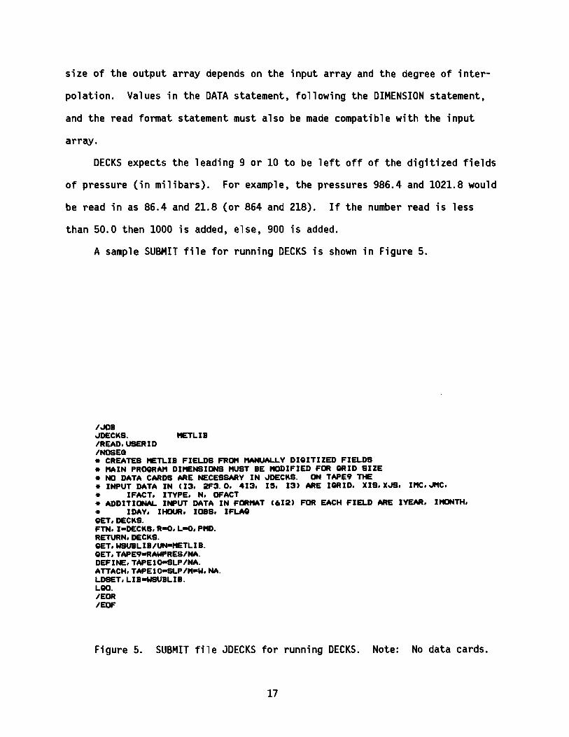
A sample SUBMIT file for running DECKS is shown in Figure 5.

I.IOBJDECKS. METLIBIREAD,USERIDINOSEG• CREATES t'lETLIB FIELDS FROt1 I1ANUALLV DIOITIZED FIELDS• f1AIN PROORN1 Dlt'lENSIDNS t1UST BE I"IODIFIED FOR ORID SIZE• NO DATA CARDS ARE NECESSARV IN JDECKS. ON TAPE9 THE• INPUT DATA IN (13. 2F3.0, 413. I'. 13) ARE IORID. XIS.XJS, I"C.~.

• IFACT. ITVPE. N, OFACT• ADDITIONAL IIIPUT DATA IN FDRttAT (612) FOR EACH FIELD ARE IVEAR. I "ONTH.• IDAV. I HOUR. lOBS. IFLAOOET. DECKS.FTN. I-DECKS.R-o,L-o.P~.RETURN. DECKS.OET,WSUBLIB/~TLIB.

OET,TAPE9-RAWPRES/NA.DEFINE,TAPElO-SLP/NA.ATTACH,TAPE10-SLP/"-W,NA.LDSET,LIB-w&UBLIB.LOO.IEORIEOF

Figure 5. SUBMIT file JDECKS for running DECKS. Note: No data cards.

17

5.3 WINDS (Calculations of Winds)

Program WINDS uses any of several models to compute surface wind fields.

Input always consists of a time series of sea-level pressures defined at each

point of a spatial grid. Models 6 and 8 also require the time sequences of

surface air temperature and air-surface-temperature difference at the grid

points. The Brown model (model 6) has the option of using dew-point depression

fields as well. The air-surface temperature difference and the dew-point

depression can be internally calculated from the surface and dew point

temperatures, respectively. The information in the file header record on

each data set (i.e., IGRID, XIS, XJS) completely defines the parameters

necessary for geometric manipulations on the polar stereographic grid. User

controlled output consists of fields of u and v components of winds and

stresses and sensible and latent heat fluxes. All the output u and v

components are relative to the grid reference frame and not the meteorological

convention of east (u) and north (v).

The input and output units are as follows:

TAPE 10

TAPE 11

TAPE 12

TAPE 13

TAPE 14

TAPE 21

TAPE 22

TAPE 23

input sea-level pressure,

input surface roughness,

input air temperature,

input air-surface temperature difference or surface

temperature,

input relative humidity, dew point, or dew-point

depression,

output u component of the surface wind (cm s-I),

output v component of the surface wind (cm s-I),

output u component of the stress (dyne cm-2), or USTAR

(cm s-l; models 6 and 8 only),

18

TAPE 24

TAPE 25

TAPE 26

output v component of the stress (dyne cm- 2), or ALPHA

(degrees; models 6 and 8 only),

output sensible heat flux (mw cm- 2), or u component

of the thermal wind (s-l), and

output latent heat flux (mw cm- 2), or v component of

the thermal wind (5-1).

Before using WINDS, the dimension of the interpolated grid should be set in the

first DIMENSION statement after the comment cards.

There are three data cards in the SUBMIT· file JWINDS (figure 6) which

control processing in the program WINDS. The first two are in free field

format meaning that the numbers must only be in the correct order and

separated by commas or spaces. Extra spaces are ignored. The cards are as

follows:

A. First card (free field format):

1. IYSTRT

2. IMSTRT

3. IDSTRT

4. IHSTRT

5. KSETS

6. MODEL

year of the start time (e.g., 81),

month of the start time,

day of the start time,

hour of the start time,

number of data sets to analyze,

model used to calculate surface winds:

=1 geostrophic winds (section 6.8),

=2 winds by the balance equation (section 6.10),

= 3 gradient winds (section 6.9),

=4 constant turning and reduction (section 6.10),

= 5 not used,

= 6 Brown model (section 6.10),

= 7 not used,

= 8 Cardone model (section 6.10);

19

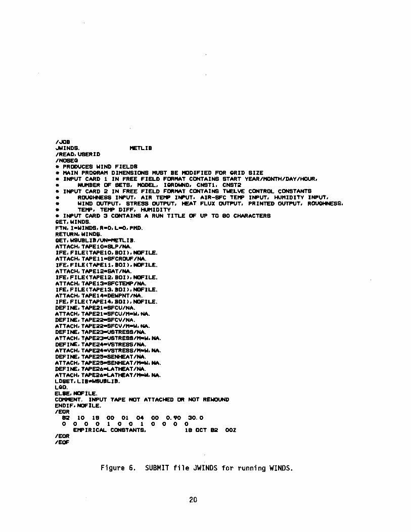
I'£TLIB

00 0.90 30.0000 0

18 OCT 82 OOZ

I.JOB"!wINDS.IREAD.UBERIDINOSEG• PRODUCES WIND FIELDS• MAIN PROQRAM DIMENSIONS MUST BE MODIFIED FOR GRID SIZE• INPUT CARD 1 IN FREE FIELD FORMAT CONTAINS START YEAR IMDNTHIDAY/HDUR.• NUMBER OF BETS. I'IDDEL. IORDWND. CNSTl,CNST2• IIIPUT CARD 2 IN FREE FIELD FORMAT CONTAINS TWELVE CONTROL CONSTANTS• ROUQHNEBS IIIPUT. AIR TEMP IIIPUT. AIR-SFC TEMP INPUT. HUMIDITY INPUT.• WIND OUTPUT. STRESS OUTPUT. HEAT FLUX OUTPUT. PRINTED OUTPUT. RD\JOHIiESS.• TEMP. TEMP DIFF. HUMIDITY• IIIPUT CARD 3 CONTAINS A RUN TITLE OF UP TO SO CHARACTERSgET. WINDS.FTN.I-WINDS.R-O.L-D.PKD.RETURN. WINDS.OET.WSUlLIB/UN-METLIB.ATTACH.TAPE10-SLP/NA.IFE.FILE1TAPE10.BOI).NDFILE.ATTACH.TAPEll-SFCRDUF/NA.IFE.FILECTAPEll.BOI).NDFILE.ATTACH. TAPE12-SAT/NA.IFE.FILECTAPE12. BOI). NDFILE.ATTACH. TAPE13-SFCTEMP/NA.IFE.FILECTAPE13.BOI).NDFILE.ATTACH. TAPE14-DEWPNT/NA.IFE. FILECTAPE14. BOI).NDFILE.DEFINE.TAPE21-sFCU/NA.ATTACH.TAPE21-SFCU/M-W.NA.DEFINE.TAPE22-sFCY/NA.ATTACH. TAPE:;Z:;Z-SFCY/M-N. NA.DEFINE.TAPE23-USTREBS/NA.ATTACH.T~E23-USTRESS/M-W.NA.

DEFINE.TAPE24-YSTRESS/NA.ATTACH. TAPE24-YSTRESS/M-W. NA.DEFINE.TAPE25-SENHEAT/NA.ATTACH.TAPE2~ENHEAT/M-W.NA.

DEFINE.TAPE26-LATHEAT/NA.ATTACH.TAPE26-LATHEAT/M-W.NA.LDBET.LIB-WSUBLIB.LOO.ELSE. NDFiLE.CDl1t£NT. INPUT TAPE NOT ATTACHED OR NOT REWOUNDENDIF. NDFILE.IEOR

BlZ 10 is 00 01 040000100 1

EMPIRICAL CONSTANTS.IEORIEOF

Figure 6. SUBMIT file JWINDS for running WINDS.

20

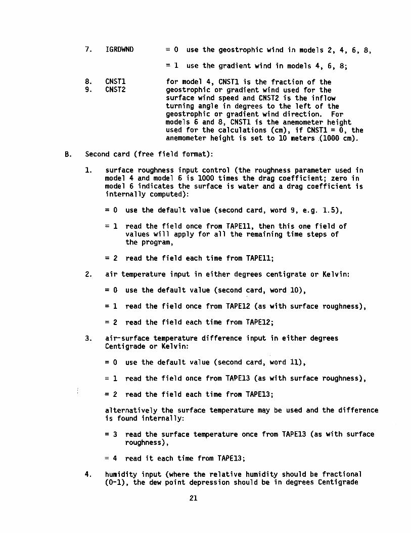
7. IGRDWND = 0 use the geostrophic wind in models 2, 4, 6, 8,

= 1 use the gradient wind in models 4, 6, 8;

CNST1CNST2

8.9.

for model 4, CNST1 is the fraction of thegeostrophic or gradient wind used for thesurface wind speed and CNST2 is the inflowturning angle in degrees to the left of thegeostrophic or gradient wind direction. Formodels 6 and 8, CNST1 is the anemometer heightused for the calculations (em), if CNST1 = 0, theanemometer height is set to 10 meters (1000 em).

B. Second card (free field format):

1. surface roughness input control (the roughness parameter used inmodel 4 and model 6 is 1000 times the drag coefficient; zero inmodel 6 indicates the surface is water and a drag coefficient isinternally computed):

=0 use the default value (second card, word 9, e.g. 1.5),

= 1 read the field once from TAPE11, then this one field ofvalues will apply for all the remaining time steps ofthe program,

= 2 read the field each time from TAPE11;

2. air temperature input in either degrees centigrate or Kelvin:

= 0 use the default value (second card, word 10),

=1 read the field once from TAPE12 (as with surface roughness),

= 2 read the field each time from TAPE12;

3. air-surface temperature difference input in either degreesCentigrade or Kelvin:

= 0 use the default value (second card, word 11),

= 1 read the field once from TAPE13 (as with surface roughness),

= 2 read the field each time from TAPE13;

alternatively the surface temperature may be used and the differenceis found internally:

= 3 read the surface temperature once from TAPE13 (as with surfaceroughness),

= 4 read it each time from TAPE13;

4. humidity input (where the relative humidity should be fractional(0-1), the dew point depression should be in degrees Centigrade

21

or Kelvin, and the dew point should be in the same units as theair temperature): .

;;: 0 use the default relative humidity (second card, word 12,e. g. 0.70),

;;: 1 read the field once from TAPE14 (as with surface roughness),

;;: 2 read it each time from TAPE14,

;;: 3 read the dew point depression field once from TAPE14 (aswith surface roughness),

;;: 4 read it each time,

;;: 5 read the dew point field once from TAPE14 (as with surfaceroughness),

;;: 6 read it each time,

5. surface wind output:

;;: 0 no output,

;;: 1 u component output on TAPE21 (cm s:~)v component output on TAPE22 (cm s );

6. stress output:

;;: 0 no output (always for models 1 and 3),

;;: 1 u component output on TAPE23 (dyne cm:~)v component output on TAPE24 (dyne cm ),

;;: 2 USTAR output on TAPE23 (cm s-1)ALPHA output on TAPE24 (degrees) (models 6 and 8, only);

7. sensible and latent heat flux or thermal wind output:

;;: 0 no output,

;;: 1 sensible heat flux output on TAPE25 (mw cm-2)latent heat flux output on TAPE26 (mw cm-2) (model 6 only),

;;: 2 u component of the thermal wind output on TAPE25 (s-1)v component of the thermal wind output on TAPE26 (s-1);

8. printed output:

=0 minimal,

;;: 1 several lines per time step,

;;: 2 several lines per grid point per time step.

22

The last four words on the second card are default values set by theuser. If a default value is used, it is assigned uniformly over thewhole field:

9. default roughness is the drag coefficient times 103 (in model 6,zero indicates an all water surface);

10. default air temperature (OC or OK);

11. default air-surface temperature difference (OC or OK);

12. default relative humidity (0-1).

C. Third card: This card is used as a run title, up to 80 characterslong.

The following three cards, for example, would process 10 sets ofdata starting at OOl 15 February 1982. Geostrophic winds would beproduced with minimal printing:

82 2 15 0 10 1 0 0 0

o 0 0 0 1 0 0 0 000 0

GEOSTROPHIC WINDS

These next three cards select the empirical constants model with 70percent reduction and 15 degrees of turning relative to the gradientwind. Stress fields are also produced using a drag coefficient of0.0015:

82 2 15 0 10 4 1 .70 15

000 0 110 0 1.5 0 0 0

EMPIRICAL CONSTANTS

And finally the Brown model is used to compute winds at a height of19.5 m from the geostrophic wind over water with input ofair temperature, sea temperature, and dew point fields at eachtime step. Winds, stress and heat flux are output:

82 2 15 0 10 6 0 1950 0

o 2 4 6

BROWN MODEL

1 110 o 0 0 0

The value for ITYPE written on the output files is

23

ITYPE = 400 + MODEL for the surface roughness parameter,

480 + MODEL for the u velocity component (em s-I),

490 + MODEL for the v velocity component (em s-I),

500 + MODEL for the u stress component, (dyne cm-2),

510 + MODEL for the v stress component (dyne cm-2),

530 + MODEL for latent heat flux (mw cm-2),

540 + MODEL for sensible heat flux (mw cm-2) ,

550 + MODEL for USTAR (em s-I),

560 + MODEL for ALPHA (~egrees),

570 + MODEL for u component of the thermal wind (s-I),

580 + MODEL for v component of the thermal wind (s-I),

so that ITYPE = 482 designates a surface u field generated by model 2.

The Brown model occasionally has problems with convergence, particularly

in unstable stratification with a strong thermal wind. If this occurs 8 line

is printed with the geostrophic wind,the air-surface temperature difference,

the thermal wind, and an LTST code with four numbers. This code is deciphered

as follows:

LTST(I) = 1

LTST(2) = 1

LTST(3) = 1

no convergence in Ultloop, test criteria increased

from 1% to 10%;

no convergence in z/L loop, test criteria increased

from 1% to 10%;

failed to converge with expanded test criteria,

horizontal temperature gradient halved;

= 2 still no convergence, quit trying; .

24 :

LTST(4) =1

= 2

no solution in subroutine PBL, horizontal temperature

gradient halved;

still no solution, quit trying.

5.4 PNTWIND (Time Series of Winds)

PNTWIND inputs the u (TAPE14) and v (TAPE15) wind components (in the

grid reference frame) and creates time series of winds at up to five specific

geographic locations by interpolation. First, the DIMENSION statement must

be adjusted for grid size. The SUBMIT file JPNTWND is shown in Figure 7.

The first data card is formatted (513,15,212) and specifies the starting

time, the data interval in hours NINT, number of data sets in the time series

KSETS, and the parameters NPT and lOUT:

NPT ... number of geographical points at which a time series is to be

created;

lOUT... specifies the type of data to be output on TAPE9 (unformatted):

lOUT = 0 for u and v components of winds (grid reference

frame),

1 for speed and direction of winds (geographic

reference frame),

2 for u and v wind components (geographic reference

frame) in IITAPE4 11 format.

25

Cards 2 through NPT+l specify the north latitude and west longitude (degrees)

of each point in (2FlO.5) format. Modifications to PNTWIND can be used to

access the u and v fields for almost any purpose.

IJOBJPNTWND. ~TLIB

IREAD,USERIDINOSEG* PRODUCES STATION TI"E SERIES FR~ ~TLIB FIELDS* ~IN PROgRA" DI"ENSIONS "UST BE "ODIFIED FOR gRID SIZE AND SERIES LENgTH* AND NUMBER OF LOCATIONS* INPUT DATA CARD 1 CONTAINS (:513, 1:5, 212) START VEARIMONTH/DAV/HOUR,* INTERVAL, SERIES LENgTH, NU"BER OF LOCATIONS, OUTPUT TVPE* SECOND AND SUCCEEDINg DATA CARDS HAVE LOCATION LAT AND LONg (2 FlO. :5)gET, PNTWIND.FTN,I-PNTWIND,R-D,L-O,PKD.RETURN, PNTWIND.gET,WSUBLIB/UN-METLIB.ATTACH,TAPE14-SFCU/NA.ATTACH,TAPE1:5-SFCV/NA.ATTACH,TAPE16-SAT/NA.ATTACH,TAPE17-SLP/NA.DEFINE,TAPE9-PNTDUT/NA.ATTACH,TAPE9-PNTOUT/NA,~W.

LDSET,LIB-WSUBLIB.LgO.IEOR

7:5 01 01 00 06 1460 2 2:57.07000 163.3300063.:50000 166.00000

IEOF

Figure 7. SUBMIT file JPNTWND for running PNTWIND.

IITAPE4 11 format was developed for time series analysis of current meter,

pressure gauge, or wind data in a set of programs known as R2D2 (see

Guide to R2D2 - Rapid Retrieval Data Display, by C. A. Pearson). IITAPE411

format consists of an unformatted nine word header field and four sets of

unformatted data arrays. If available, the temperature and pressure fields

are assigned to TAPE16 and TAPE17, respectively. The header field created is:

26,. .... ;4f •.

....

Word Description Content

1 grid type "METLIB",IGRID,IFACT

2 model number ITYPE

3 height always "0"

4 start time YYJJJHHMM

5 end time YYJJJHHMM

6 seri es 1ength . KSETS

7 data time interval, minutes NINT*60

8 north latitude, decimal degrees ALAT

9 west longitude, decimal degrees ALON

Start time and end time are written as nine digit integers YYJJJHHMM where YY

is year, JJJ Julian day, HH hour, and MM minutes. The data arrays are written

to TAPE9 in order of east velocity, north velocity, temperature and pressure

(the latter two arrays are zero-filled if data are unavailable). Data are

written in arrays of maximum size 2000. If the actual series length is

larger than 2000, the first 2000 values of all the parameters are written in

the above order, then the next 2000, etc.

5.5 TRKWIND (Time Series of Winds Following a Track Line)

TRKWIND inputs up to four METLIB grid variables and creates time series

of these variables along a user-specified time series of geographic positions.

This program is thus helpful for generating wind, temperature, and/or pressure

time series along the route of a steaming ship, drifting buoy, etc.

27

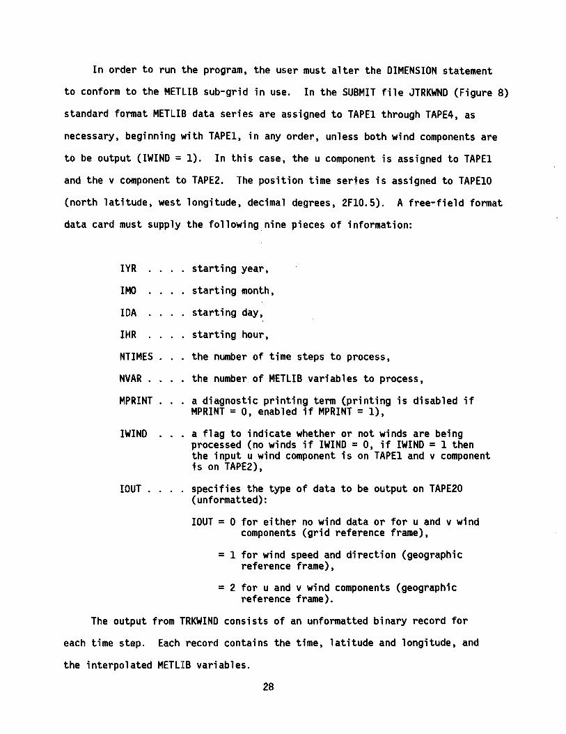
In order to run the programs the user must alter the DIMENSION statement

to conform to the METLIB sub-grid in use. In the SUBMIT file JTRKWND (Figure 8)

standard format METLIB data series are assigned to TAPE1 through TAPE4 s as

necessarys beginning with TAPE1 s in any orders unless both wind components are

to be output (IWIND = 1). In this cases the u component is assigned to TAPE1

and the v component to TAPE2. The position time series is assigned to TAPElO

(north latitudes west longitudes decimal degrees s 2F10.5). A free-field format

data card must supply the following nine pieces of information:

IYR

lHO

IDA

r~R

NTIMES .

starting years

. starting months

starting days

starting hours

the number of time steps to process s

NVAR .... the number of METLIB variables to process s

MPRINT . a diagnostic printing term (printing is disabled ifMPRINT =Os enabled if MPRINT =l)s

IWIND a flag to indicate whether or not winds are beingprocessed (no winds if IWIND =Os if IWIND =1 thenthe input u wind component is on TAPE1 and v componentis on TAPE2L

lOUT . . . . specifies the type of data to be output on TAPE20(unformatted):

lOUT =0 for either no wind data or for u and v windcomponents (grid reference frame)s

=1 for wind speed and direction (geographicreference frame)s

=2 for u and v wind components (geographicreference frame).

The output from TRKWIND consists of an unformatted binary record for

each time step. Each record contains the times latitude and longitudes and

the interpolated METLIB variables.

28

I.JOB~TRKWND. METLIBIREAD.USERIDINOSEO* INTERPOLATES METLIB FIELDS TO A TRACK LINE* ""IN PRogRAM DIMENSIONS MUST BE MODIFIED FOR GRID SIZE* INPUT IN FREE FIELD FORMAT START YEAR. MONTH. DAY. HOUR.* NUMBER OF TIME STEPS. NUMBER OF VARIABLES. PRINT ENABLER.* A FLAg FOR PROCESSINO WIND DATA. AND A SPECIFICATION OF* THE FORM OF WIND OUTPUT.gET. TRKWIND.FTN.I-TRKWIND.R-D.L-O.PKD.RETURN. TRKWIND.gET.WSUBLIB/UN-METLIB.ATTACH.TAPE1-SFCU/NA.IFE.FILE(TAPE1.MS).NOFILE.ATTACH.TAPE2-SFCV/NA.IFE.FILE(TAPE2.MS).NOFILE.ATTACH.TAPE3-SLP/NA.IFE.FILE(TAPE3.MS).NOFILE.ATTACH.TAPE4aSAT/NA.IFE.FILE(TAPE4.MS).NOFILE.gET.TAPE10-BHIPTRK.IFE.FILE(TAPE10.MS).NOFILE.DEFINE.TAPE20-TRAKOUT/NA.ATTACH. TAPE2D-TRAKOUT/M-W. NA.LDSET.LIB-WSUBLIB.LgO.ELSE. NOFILE.COMMENT. INPUT DATA FILE NOT FOUNDENDIF. NOFILE.IEDR7:t. 1. 1. O. :tOO. 4. O. 1. 1

IEOF

Figure 8. SUBMIT file JTRKWND for running TRKWIND.

5.6 METlOOK (Pri nts Records from METLIB Fi 1es)

METlOOK reads and prints the header record and the first. last. and any

chronologically-ordered. user-specified data records from an unformatted

binary METlIB file. Up to four files may be processed. The data grid may be

as large as 63 x 63 without modifying this routine. The input files are

assigned to logical units 11 through 14 (TAPEll. etc.; Figure 9). as required.

User-requested record dumps require one data card for each record (free field

format) :

29

IUNIT

IYR

IMO

IDA

IHR

the num~er of the logical unit on which the data reside.

. the year of the user-requested data record

to be d~mped.

the month of the data record.

the day of the data record.

the hour of the data record.

I.JOB.Jt1ETLDK. I'1ETLIIIREAD,USERIDINOSEG• PRINTS ~LII FIELDS• MAIN PRDQRAM NEEDS NO MODIFICATION IF QRID IS NOT LARGER THAN 63 X 63• HEADER RECORD AND FIRST, LAST, AND USER SPECIFIED DATA RECORDS ARE LISTED• FROM AS MANY AS FOUR SEPARATE METLII FIELDS (TAPE11, 1~, 13. 14)• INPUT DATA IN FREE FJELD FORMAT ARE CHRONOLOGICALLY ORDERED USER SPECIFIED• DATA TIMES FOR IUNIT. YEAR. MONTH. DAY, HOUR. ONE CARD FOR EACH TIME.GET,METLOOK/UN-METLIB.FTN,I-METLOOK,R-o,L-O,PMD.RETURN,I'IETLOOK.ATTACH,TAPEI1-SFCU.IFE,FILE(TAPEll,MS),NOFILE.ATTACH.TAPE1~-SFCY.

IFE,FJLE(TAPE1~,MS),NOFILE.

ATTACH,TAPEI3-sLP.JFE.FILE(TAPEI3,MS),NOFJLE.ATTACH, TAPEI4-SAT.IFE,FILE(TAPEI4,MS),NOFILE.LGO.ELSE, NOFILE.CCII'V1ENT. INPUT DATA FILE NOT FOUNDENDIF, NOFJLE.lEaR11,66,10,1,011, 66, 11, 1, 011,67,10,1,0

IEOF

Figure 9. SUBMIT file JMETlOK for running METlOOK.

5.7 FORMAT (Creates formatted files from METlIB files)

It is sometimes necessary to transfer METlIB data files to different

computing installations. Standard METlIB files are generated by unformatted

30

binary WRITE statements, and these files are not easily read by different

computing systems. FORMAT is a utility program which converts standard

METLIB files to formatted files which can be transferred to other installations.

In order to run FORMAT, it is not necessary to modify the program if the

data grid to be converted is no larger than 65 x 65. By default, FORMAT will

process one METLIB file assigned to TAPE1, writing the formatted output to

TAPE2 with the header record in format (13, 2F3.0, 413, 15, 13) and each data

record as one line of time and data characteristics (612) followed by as many

lines as necessary of (10E12.5) to output the grid variables. These formats

were chosen to match the input header cards of the program DECKS.

In the SUBMIT file ~IFORMAT (figure 10) the user may override these

default settings by providing as many as four data cards: the first specifying

in free field format the number of files to process from the TAPE1 input unit

(NFILS), and the final three cards specifying the number of format characters

(NCHAR) and the formats for the header (IHDRFMT), time (ITIMFMT), and data

(IDATFMT) records, respectively. The format for typing these three data

cards is (13, 77A1). If a substitution is made for a default parameter, all

the data cards preceding the substitution must be entered with their default

values. The data cards following the substitution do not need to be entere~.

For example, if the time and data characteristics are to be written in (313,

214, 12) instead of (612) the data file would contain the first two cards

with their default values then the card with the substituted format

specification:

1

14(13,2F3.0,413,15,13)

12(313,214,12).

31

IJOB.,/FORMAT. ~TLIB

IREAD,PIHEADI~CI

• WRJTI8 FOR"ATTED ~TLIB FILES FROI1 IJIlFORr1ATTED BINARV INPUT• PRDORN1 NEEDS NO I'IDDIFICATION IF DATA GRID IS NO LARGER THAN 6~ X 6~

• NO ~TA CARDS ARE NECESSARV, HOWEVER.• US~ft MAV OVERRIDE NUI'IBER OF FILES AND OUTPUT FORr1AT DEFAULT BV SPECIFVING• DAT~ CARD 1 (FREE FIELD FORr1AT> NFILS. CARD 2 <l3.77AU NCHAR.IHDRFr1T.• CARD 3 (I3.77Al) NCHAR,ITIr1Fr1T, CARD 4 (I3.77A1) NCHAR.IDATF"T~ET. FPRr1AT.FTN. J~ORKAT.R.O.L-o.P"O.ATTACH,TAPE1.BPB3/UN-YLL.~.

DEFINE,TAPE3·PBERB3/~.

ATTACH,TAPE3aPBERB3/r1aW.~.LQO.REWIND, TAPE2.COPV! I , TAPE2. TAPE3.REWIND, TAPE3.PACK, T~E3.IEDRIEOF

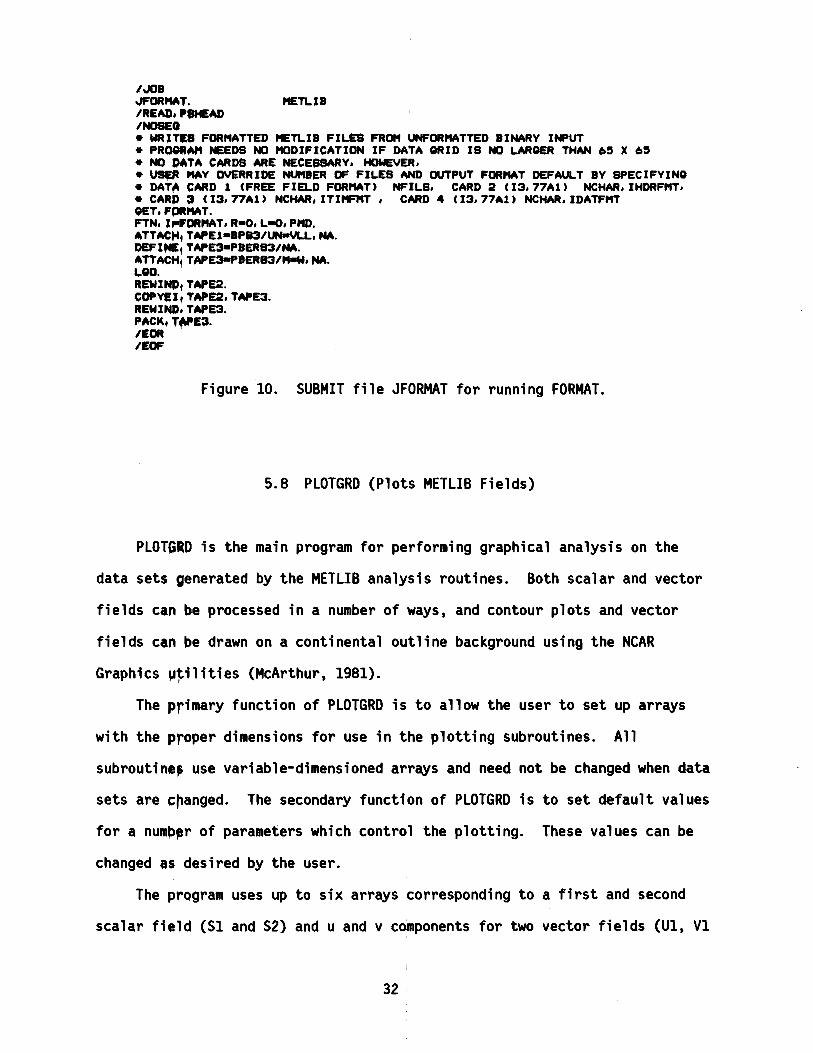
Figure 10. SUBMIT file JFORMAT for running FORMAT.

5.8 PlOTGRD (Plots MElLIB Fields)

PlOTGRD is the main program for performing graphical analysis on the

data sets generated by the METlIB analysis routines. Both scalar and vector

fields can be processed in a number of ways, and contour plots and vector

fields can be drawn on a continental outline background using the NCAR

Graphics ~~ilities (McArthur, 1981).

T~e primary function of PlOTGRD is to allow the user to set up arr~s

with the proper dimensions for use in the plotting subroutines. All

SUbroutine, use variable-dimensioned arr~s and need not be changed when data

sets are c~anged. The secondary function of PlOTGRD is to set default values

for a nump,r of parameters which control the plotting. These values can be

changed as desired by the user.

The program uses up to six arrays corresponding to a first and second

scalar field (51 and 52) and u and v components for two vector fields (U1, VI

32

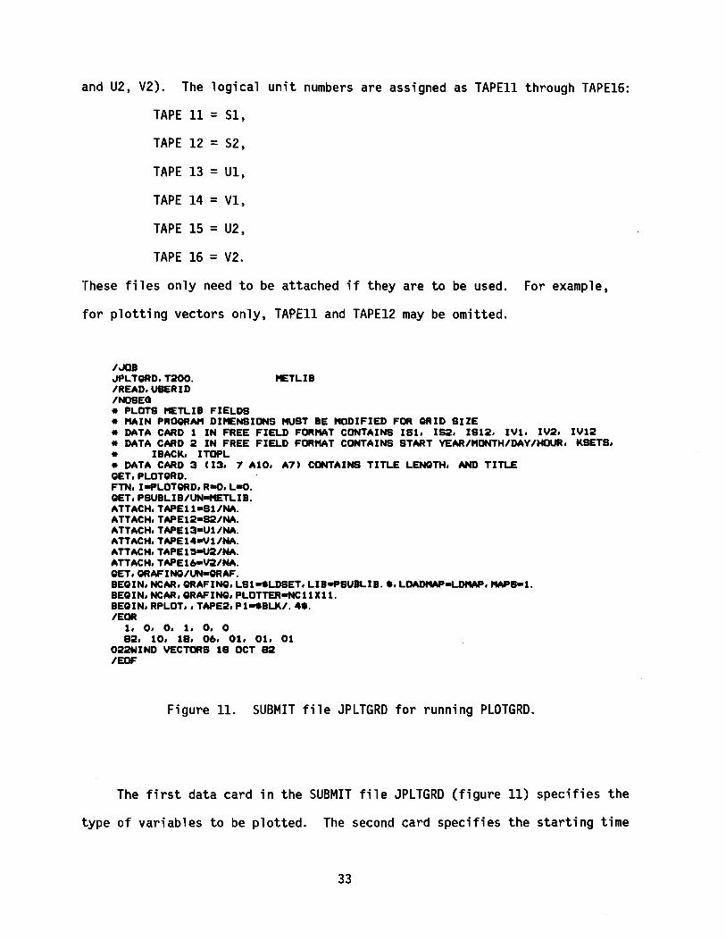
and U2, V2). The logical unit numbers are assigned as TAPE11 through TAPE16:

TAPE 11 =51,

TAPE 12 =52,

TAPE 13 =U1,

TAPE 14 =VI,

TAPE 15 =lI2,

TAPE 16 = V2.

These files only need to be attached if they are to be used. For example,

for plotting vectors only, TAPE11 and TAPE12 may be omitted.

1.J08JPLTQRD.T200. METLI8IREAD.UBERIDINOSEG* PLOTS METLI8 FIELDS* "AIN PROQR~ DIMENSIONS ~ST 8E MODIFIED FOR QRID SIZE* DATA CARD 1 IN FREE FIELD FOR~T CONTAINS IS1. lea. IS12. IV1. IV2. IV12* DATA CARD 2 IN FREE FIELD FOR~T CONTAINS START VEAR/"ONTH/DAV/HOUR. KSETS.* I8ACK. ITOPL• DATA CARD 3 (13. 7 Al0. A7) CONTAINS TITLE LENOTH. AND TITLEGET. PLOTQRD.FTN,I-PLOTQRD,RaO,L-O.QET,PSU8LI8/UN-HETLI8.ATTACH,TAPEll-Sl/NA.ATTACH,TAPE12-S2/NA.ATTACH,TAPE13-Ul/NA.ATTACH,TAPE14-Vl/NA.ATTACH,TAPE1~-U2/NA.

ATTACH, TAPE16-V2/NA.QET,QRAFINQ/UN-QRAF.8EQIN,NCAR,QRAFINQ,LS1"LDSET,LI8.pSU8LI8.*,LOADKAP-LDKAP,~8-1.

8EQIN,NCAR,QRAFINQ,PLOTTER-NCllXll.8EQIN,RPLOT"TAPE2,Pl..8LK/.4*.IEOR

1, 0, 0, 1, 0, 082, 10, 18, 06, 01, 01, 01

022WIND VECTORS 18 OCT B2lEaF

Figure 11. SUBMIT file JPLTGRD for running PLOTGRD.

The first data card in the SUBMIT file JPLTGRD (figure 11) specifies the

type of variables to be plotted. The second card specifies the starting time

33

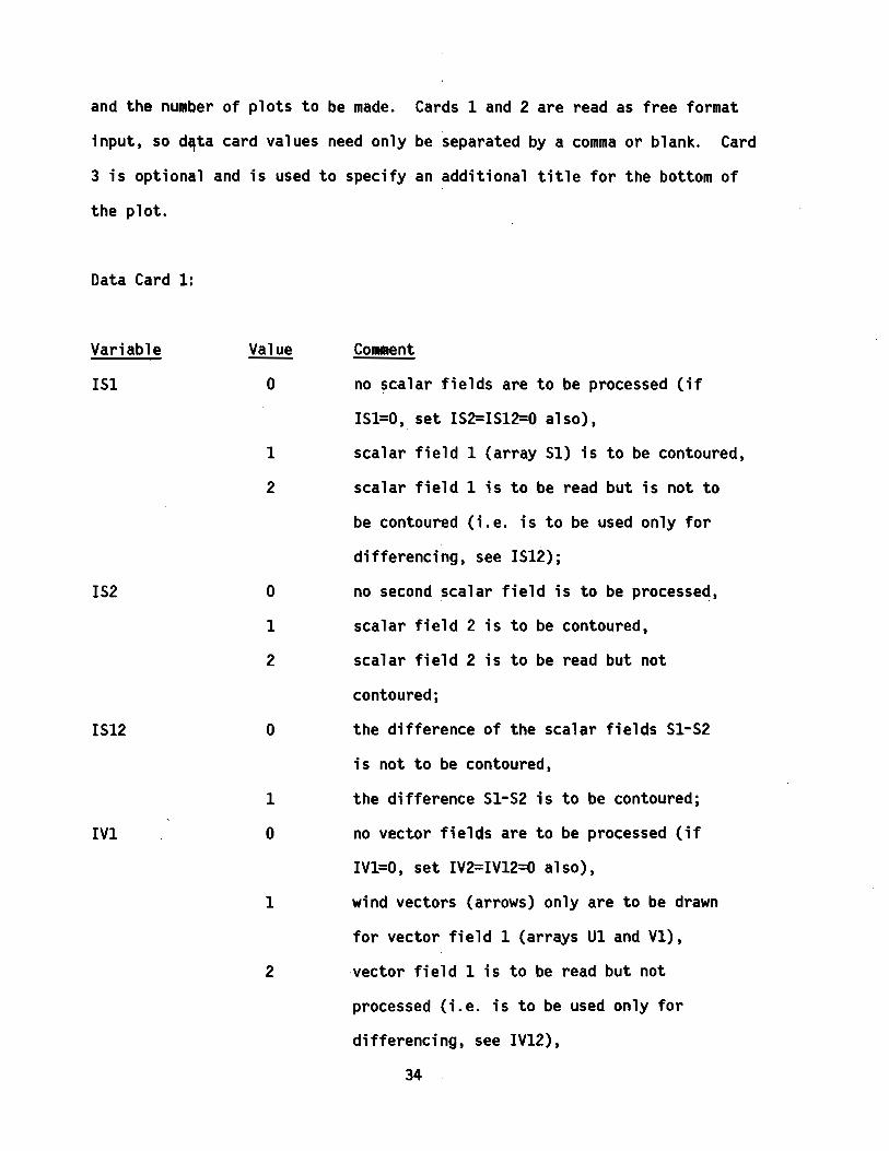
and the number of plots to be made. Cards 1 and 2 are read as free format

input, so d~ta card values need only be separated by a comma or blank. Card

3 is optional and is used to specify an additional title for the bottom of

the plot.

Data Card 1:

Variable

151

152

1512

1Vl

Value

o

1

2

o

1

2

o

1

o

1

2

Comment

no scalar fields are to be processed (if

151=0, set 152=1512=0 also),

scalar field 1 (array 51) is to be contoured,

scalar field 1 is to be read but is not to

be contoured (i.e. is to be used only for

differencing, see 1512);

no second scalar field is to be processed,

scalar field 2 is to be contoured,

scalar field 2 is to be read but not

contoured;

the difference of the scalar fields 51-52

is not to be contoured,

the difference 51-52 is to be contoured;

no vector fields are to be processed (if

1V1=O, set 1V2=IV12=0 also),

wind vectors (arrows) only are to be drawn

for vector field 1 (arrays U1 and VI),

vector field 1 is to be read but not

processed (i.e. is to be used only for

differencing, see 1V12),

34 i

IV2

IV12

3

4

o

1

2

3

4

o1

2

3

isotachs (contours of the magnitude of the

vectors. ex. wind speed) only of vector field 1

are to be drawn.

both 1 and 3. i. e.• both arrows and

isotachs of vector field 1 are to be drawn;

no vector field 2 is to be processed (if

IV2=O. set IV12=O also).

wind vectors (arrows) only are to be drawn

for vector field 2 (arrays U2 and V2).

vector field 2 is to be read but not

processed (i.e. is to be used only for

differencing. see IV12).

isotachs only of vector field 2 are to be

drawn.

both 1 and 3. i. e.• both arrows and

isotachs of vector field 2 are to be drawn;

no differencing of vector fields is to be done,

arrows only of vector field 1 minus vector

field 2 are to be drawn.

isotachs only of the magnitude of vector field 1

minus the magnitude of vector field 2 are to be

contoured,

both 1 and 2, i.e. arrows and isotachs of the

differences.

35

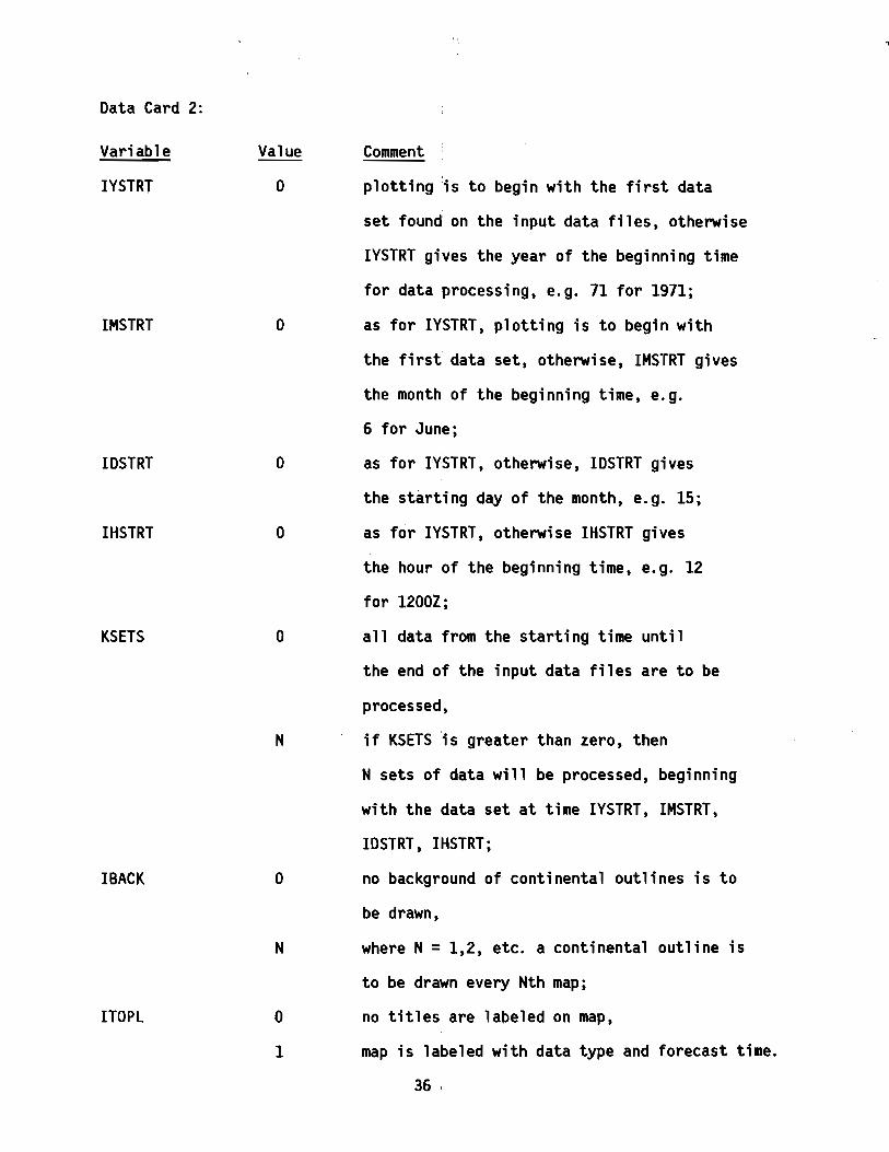
Data Card 2:

Variable

IYSTRT

IMSTRT

IDSTRT

IHSTRT

KSETS

IBACK

ITOPL

Value

o

o

o

o

o

N

o

N

o

1

Comment

plotting is to begin with the first data

set found on the input data files, otherwise

IYSTRT gives the year of the beginning time

for data processing, e.g. 71 for 1971;

as for IYSTRT, plotting is to begin with

the first data set, otherwise, IMSTRT gives

the month of the beginning time, e.g.

6 for June;

as for lY'STRT, otherwi se, IDSTRT gi ves

the starting day of the month, e.g. 15;

as for IYSTRT, otherwise IHSTRT gives

the hour of the beginning time, e.g. 12

for 12002;

all data from the starting time until

the end of the input data files are to be

processed,

if KSETSis greater than zero, then

N sets of data will be processed, beginning

with the data set at time IYSTRT, IMSTRT,

IDSTRT, IHSTRT;

no background of continental outlines is to

be drawn,

where N=1,2, etc. a continental outline is

to be drawn every Nth map;

no titles are labeled on map,

map is labeled with data type and forecast time.

36 '

Note that setting IYSTRT=IMSTRT=IDSTRT=IHSTRT=KSETS=O means that all data

found on the input files will be processed.

Data Card 3: This card provides any desired title at the bottom of the plot,

given the specification of 2 variables:

Variable

NAUXTL

AUXTIT

Format

13

7A10,A7

Comment

the number of characters in the

auxiliary title;

the character string which comprises the

title (up to 77 characters are allowed).

If no auxiliary title is desired, either omit this data card entirely or give

NAUXTL the value O. An example of data card 3 is: 013EXAMPLE TITLE.

Figure 12 is a sample plot.

The next set of variables is assigned within PLOTGRD and can be changed

by editing a copied version of the program:

JGRID .... the interval for drawing latitude and longitude lines,

default is 10°;

IUSOUT.... determines whether or not U.S. state outlines are to be

drawn if continental outlines are drawn, default of 1

gives state outlines, set to 0 for no outlines;

lOOT..... 0 for continental outlines drawn by solid lines (default),

1 for continental outlines drawn by dotted lines;

NHI ..... 0 if highs and lows are labelled by Hand L on all contour

maps (pressure maps are always labelled Hand L),

-1 if highs and lows are not to be labelled (default).

37

--......-.....

......-

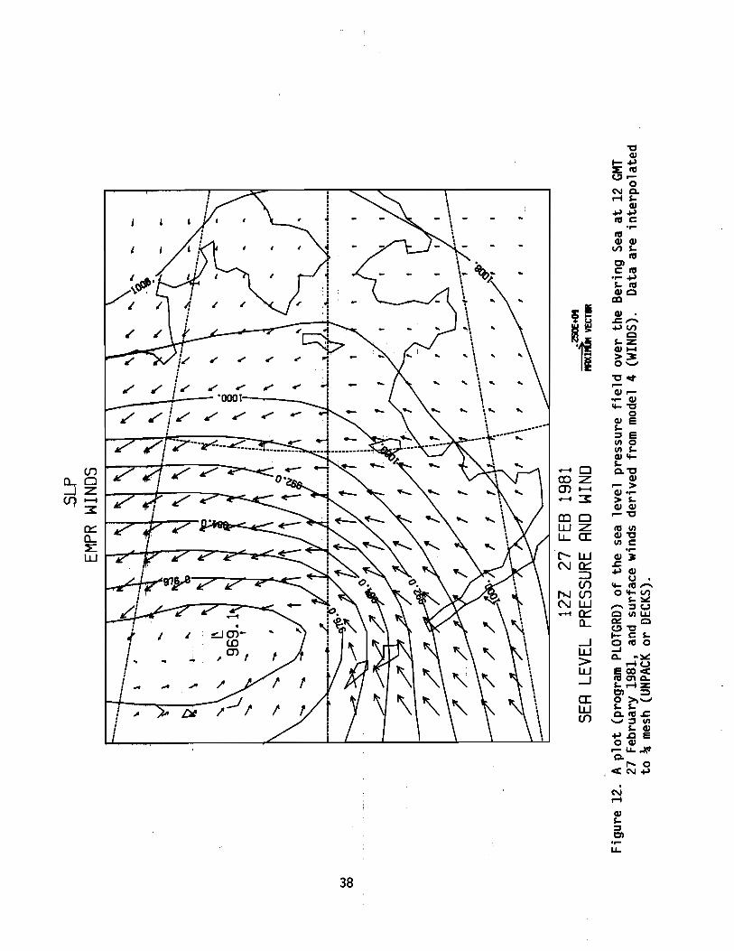
...f

1---:--~-

w ())

\.....

1-..

.

-SlP

EMPR

WIN

DS

'\ \" ----- '\

\,

'\I.'

,0 0 '1'

,\

\,

1,

,~!

__---

-f----

-;---

\_

__-_

..---

---1':

,,

,,

\ \ 1\

,,

\ \

12Z

27FE

B19

81SE

ALE

VEL

PRES

SURE

AND

WIN

D.Z

SlE

+04

tllX

IItl

.VE

CTIR

Fig

ure

12.

Ap

lot

(pro

gram

PLOT

GRD)

ofth

ese

ale

vel

pres

sure

fiel

dov

erth

eB

erin

gSe

aat

12GM

T27

Febr

uary

1981

.an

dsu

rfac

ew

inds

deri

ved

from

mod

el4

(WIN

DS)

.D

ata

are

inte

rpo

late

dto

~m

esh

(UNP

ACK

or

DEC

KS)

.

Contour intervals for various types of data are as follows:

PRESIN.

TEMPIN.

the contour interval for pressure fields, default is 4.0 mb;

the contour interval for temperature fields, the default

is 1.00 C;

WINDIN.... the contour interval for isotachs of the wind fields,

default is 400.0 cm sec-I;

OTHRIN the contour interval for any other data type, the

default of 0.0 allows the NCAR routine to examine

the data and choose an appropriate interval.

Contour intervals for plotting the differences between two data fields

are as follows:

PDIFIN.... the contour interval for contouring the differences of

two pressure fields, default is 2.0 mb;

TDIFIN.... the interval for contouring the difference of two

temperature fields, default is 1.00 C;

WDIFIN.... the interval for contouring isotachs of the difference

of two vector fields, default is 200.0 cm sec-I;

ODIFIN.... the interval for contouring differences of other types

of data, the default is 0.0.

Any of these eight contour intervals can be set to zero, as are OTHRIN

and ODIFIN. If this is done, the NCAR plot routines select an appropriate

interval.

Parameters for the wind vector (arrow) plots are:

39

VECMIN .... the smallest vector magnitude to be drawn t default

is 0.0;

VECMAX .... the largest vector magnitude to be drawn t the plot

is scaled so that an arrow of this length will just

reach from one data point to the next t default is

2500.0 cm sec-I;

VDIFMN .... the smallest vector magnitude to be drawn when the

difference of two vector fields is being plotted t any

vector smaller than this will not be plotted t default-1is 1.0 cm sec ;

VDIFMX .... the largest vector magnitude to be drawn when the

difference of two vector fields is being plotted t

default is 500.0 cm sec-I.

If the wind is greater than VECMAX t only a point is plotted; if the wind is

less th~n or equal to VECMIN no mark is plotted at the grid point.

5.9 DRAWMAP

Thi$ program creates plots of the polar stereographic background used

with PLOTGRD. DRAWMAP is run by JDRWMAP (Figure 13) and generates working

base map$ for hand plotting and analyzing meteorological data for later

digitization. The data card is described in section 4.

40

I JOB~DRWKAP. ~TLIB

IREAD,USERIDINOSEG* DRAWS A SPECIFIED QRID OR SUBQRID* MAIN PROQRAM NEEDS NO MODIFICATION* USER INPUTS IN FREE FIELD FORMAT IQRID, XIS, XJ6, IMC, ~C, IFACTQET,DRAWMAP/UN-METLIB.FTN,I-DRAWMAP,R-O,L-O.RETURN, DRAWMAP.QET,QRAFINQ/UN-QRAF.QET,WSUBLIB/UN-METLIB.BEQIN,NCAR,QRAFINQ,MAPS-2,LS1-.LDSET,LIB-WSUBLIB.•.BEQIN,NCAR,QRAFINQ,PLOTTER-NCllXll,LDADKAP-O.BEQIN,RPLOT"TAPE2,Pl-.BLK/.3•.IEOR

I, 1., 1., 6', 6', 1IEOF

Figure 13. SUBMIT file JDRWMAP for running DRAWMAP.

6. SUBROUTINE DOCUMENTATION

6.1 Introduction

The bulk of the computations performed by METlIB-II are accomplished by

its many subroutines. Since the source code of these subroutines is invariant,

they are pre-compiled. The resulting relocatable code is stored in two

subroutine libraries: WSUBlIB contains routines supporting computational

programs such as UNPACK and WINDS, while the plotting programs access the

PSUBlIB subroutine library. A list of subroutines contained in WSUBlIB with

abbreviated documentation can be found in section 6.2. PSUBlIB makes extensive

reference to the NCAR Scientific Computing Division Graphics package (McArthur,

1981). Consult the authors of METlIB-II for source listings and calling

sequences.

41

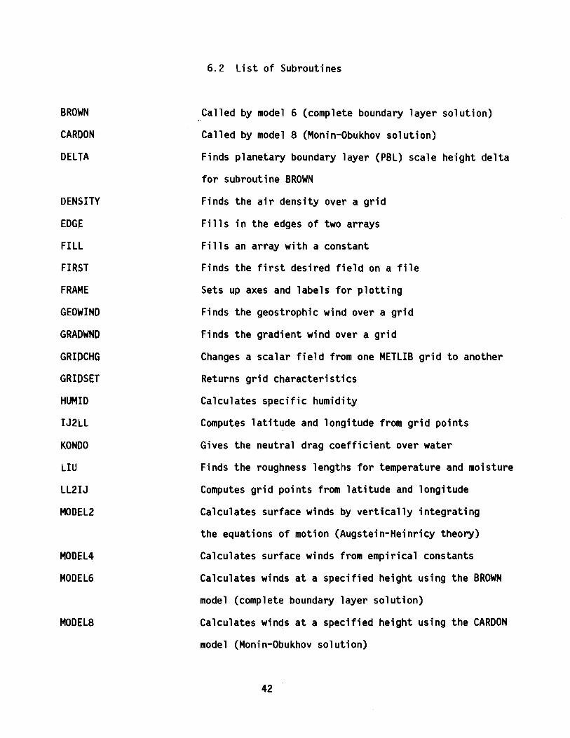
BROWN

CARPON

DELTA

DENSITY

EDGE

FILL

FIRST

FRA~E

GEOWIND

GRADWND

GRIDCHG

GRIDSET

HUMID

IJ2LL

KONDO

LIU

LL2IJ

MODEL2

MODEL4

MODEL6

MODEL8

6.2 List of Subroutines

Called by model 6 (complete boundary layer solution)

Called by model 8 (Monin-Obukhov solution)

Finds planetary boundary layer (PBL) scale height delta

for subroutine BROWN

Finds the air density over a grid

Fills in the edges of two arrays

Fills an array with a constant

Finds the first desired field on a file

Sets up axes and labels for plotting

Finds the geostrophic wind over a grid

Finds the gradient wind over a grid

Changes a scalar field from one METLIB grid to another

Returns grid characteristics

Calculates specific humidity

Computes latitude and longitude from grid points

Gives the neutral drag coefficient over water

Finds the roughness lengths for temperature and moisture

Computes grid points from latitude and longitude

Calculates surface winds by vertically integrating

the equations of motion (Augstein-Heinricy theory)

Calculates surface winds from empirical constants

Calculates winds at a specified height using the BROWN

model (complete boundary layer solution)

Calculates winds at a specified height using the CARDON

model (Monin-Obukhov solution)

42

NTERP Interpolates a field to a point

PBl Boundary layer model called by subroutine BROWN

PRNTOUT Prints entire fields as calculated in program WINDS

PSU, PHU, PSI. PST, etc. Surface layer parameter functions

ROUGH Gives the roughness length

SD2UV Computes u and v components from speed and direction

SMOGRD Smooths or desmooths grid

THRMWND Finds the thermal wind over a grid

UV2SD Computes speed and direction from u and v components

ZETA Finds the stability parameter

6.3 Interpolation (NTERP)

NTERP is a general subroutine for interpolating values to an arbitrary

fractional I-J location from a regular grid-point array. To call NTERP,

first determine whether the point is closer than one grid from a boundary.

in which case the value is assigned via linear interpolation (i.e. KQUAD=5).

For an interior point, biquadratic interpolation is used. which utilizes

the values at the 16 surrounding points and is consistent with procedures

in use at the National Meteorological Center (NMC).

6.4 location on Subgrid (IJ2ll,ll2IJ)

IJ2ll calculates the latitude. ~, and longitude. A, from polar

stereographic grid locations. The transformation equations are:

43

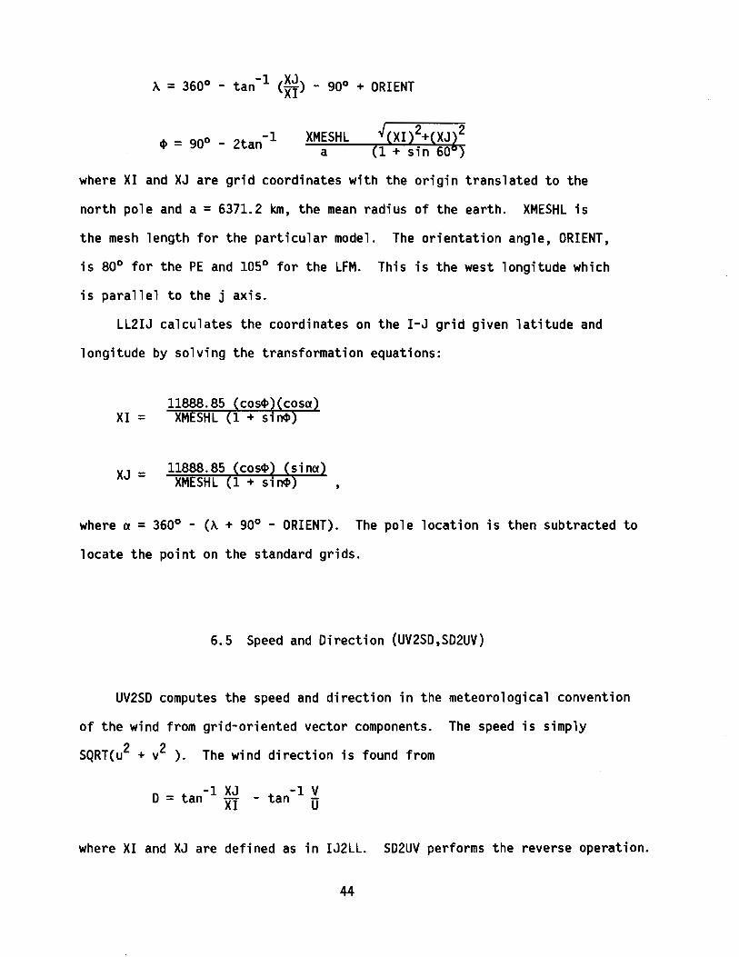
A = 360° - tan-1 (XJ) - 90° + ORIENTXI

-1~ = 90° - 2tan XMESHL

a (1 + sin 60 )

where XI and XJ are grid coordinates with the origin translated to the

north pole and a = 6371.2 km, the mean radius of the earth. XMESHL is

the mesh length for the particular model. The orientation angle, ORIENT,

is 80° for the PE and 105° for the LFM. This is the west longitude which

is parallel to the j axis.

LL2IJ calculates the coordinates on the I-J grid given latitude and

longitude by solving the transformation equations:

11888.85XI = XMESHL

XJ =

where a = 360° - (A + 90° - ORIENT). The pole location is then subtracted to

locate the point on the standard grids.

6.5 Speed and Direction (UV2SD,SD2UV)

UV2SD computes the speed and direction in the meteorological convention

of the wind from grid-oriented vector components. The speed is simply

SQRT(u2 + v2 ). The wind direction is found from

-1 XJ -1 VD = tan XI - tan U

where XI and XJ are defined as in IJ2LL. SD2UV performs the reverse operation.

44

6.6 Thermal Wind (THRMWND)

This subroutine calculates the non-dimensional thermal u and v wind

component fields. These calculations are made only if one of models 6 or 8 is to

be used or if it is specified in word 7 of the second input card to program WINDS.

The vertical gradient of the geostrophic wind in the boundary layer is assumed

to depend only on the surface horizontal temperature gradient computed by

central differences and on the Coriolis parameter:

V - 9­T = 2­f T

aTax

where g is the gravitational acceleration; f, the Coriolis parameter; and

air temperature (SAT) is taken for the boundary layer average temperature, T,at each grid point.

6.7 Grid Initialization (GRIDSET)

GRIDSET reads in IGRID, IFACT, and other parameters and adjusts them

according to the degree of interpolation and the grid system used.

6.8 Geostrophic Wind (GEOWIND,EDGE)

In order to compute geostrophic wind, the components of the pressure

gradient at each point of a grid field are found by central differences,

dividing by twice the earth distance between adjacent grid points at that

latitude. The grid spacing distance, the Coriolis parameter, and the air

45

density depend on the grid point. Subroutine EDGE assigns values to the

boundary points from the closest interior points.

To generate geostrophic winds. the program WINOS (section 5.3) requires

the pressure input on TAPElO and the wind components (cm s-l) output on TAPE21

and TAPE22 in JWINDS. The first data card must have word 6 (MODEL) set to 1

and w9rd 7 (IGRDWND) set to 0; in addition. word 5 on card 2 must be set to 1.

6.9 Gradient Wind (GRADWND)

A method of successive approximations is used for computing the gradient

wind at each interior point (Endlich. 1961). In GRADWND the geostrophic windI

speed and the radius of ¢urvature are calculated at each point. The equation

C =C - C2 is iterated. where C is the gradient wind speed. C is theg fr g

geostrophic wind speed. f is the Coriolis force. and r is the radius of the

curvature (negative for a clockwise trajectory). EDGE is called at the end

to assign gradient wind values to perimeter points.

For gradient wind o~tput from WINDS. the submit file JWINDS must have

the pressure input on TAPE10 and the wind components (cm s-l) output on TAPE21i

and TAPE22; word 6 and word 7 on the first data card are set to 3 and 1

respectively; and word 5 on the second data card is set to 1.

6.10 Wind Models (MODEl2. 4. 6. 8. BROWN. CARDON. etc.)

There are four options available for modeling surface winds in the METlIB

program WINDS. They are chosen by setting word 6 on the first data card inI

46

JWINDS. It is imperative to note that all u and v components are relative to

the reference grid and not meteorological convention.

Model 4 calculates a surface wind from the geostrophic or gradient wind

by reducing the wind speed and rotating the wind direction by the amounts

specified in CNSTI and CNST2 on the first data card in JWINDS. If CNST2 is

positive, the rotation is to the left of the geostrophic (or gradient) wind.

The surface stress may be calculated using a constant drag coefficient (set

in word 9 of data card 2 in JWINDS). Surface wind components (cm s-l) are

output to TAPE21 and TAPE22 by setting word 5 of card 2 to 1. When word 6 of

card 2 is set to 1, the u and v components of surface stress (dyne cm-2) are

written to TAPE23 and TAPE24.

Model 2 utilizes the vertically intergrated equations of motion, as

suggested by Mahrt (1975) and by Augstein and Heinricy (1976), to yield a

first-order approximation of surface winds from geostrophic winds. The

equations are discussed in the original METLIB manual (Overland, et a1.,

1980). The output of surface wind and/or surface stress components is

controlled by setting words 5, 6, and 9 on card 2 in JWINDS.

Models 6 and 8 are full single point atmospheric-boundary-1ayer models

that compute the thermal wind from surface air temperature fields then use

the thermal wind, the air-sea temperature difference, and the latitude to

correct for stability and baroc1inity of the boundary layer in deriving

surface-wind speed and inflow angle from the geostrophic or gradient wind.

MODEL6 uses the model of R. A. Brown (subroutine BROWN), summarized in

Appendix A of the original METLIB manual (Overland et a1., 1980). The model

is also described by Brown and Liu (1982). MODEL8 uses the model provided by

V. Cardone (subroutine CARDON), summarized in Appendix B of the original

METLIB manual.

47

Models 6 and 8 utilize the geostrophic (or gradient) and thermal winds,

relative humidity or dew point depression (model 6 only), and air-surface

temperature difference calculated in WINDS to compute a variety of surface

layer parameters at the height CNST1 (cm, word 8 of card 1 in JWINDS).

The second data card in JWINDS controls the output of models 6 and 8

including the u and v wind components (cm s-l, word 5 =1) on TAPE21 and

TAPE22, either the u and v stress components (dyne cm- 2, word 6 = 1) or USTAR

and ALPHA (cm s-l and degrees, respectively, word 6 = 2) on TAPE23 and TAPE24,

and (for model 6 only) the sensible and latent heat fluxes (mw cm-2, word 7 =1)

on TAPE25 and TAPE26. In both models, USTAR is the friction velocity defined

as ~stressJair density and ALPHA is the turning angle between the geostrophic

(or gradient) wind and USTAR. When ALPHA is positive the turning is to the

left of the input wind signifying inflow toward a northern hemispheric low

pressure center.

48

7. ACKNOWLEDGEMENTS

This report is a contribution to the Marine Services Project at Pacific

Marine Environmental Laboratory. It has been funded in part by the Fisheries

Oceanography Coordinated Investigations (FOCI). Subroutines IJ2LL, LL2IJ,

and NTERP are adaptations of subroutines in use at the National Meteorological

Center. Our thanks to J. E. Overland, S. Galt, V. L. Long, and C. H. Pease

who have contributed to the development of METLIB-II. We are indebted to

Ryan Whitney and Lai Lu for their help in preparing this manuscript.

49

8. REFERENCES

Augstein, E. and D. Heinricy (1976): Actual and geostrophic wind relationships

in an accelerated marine atmospheric boundary layer. Beitrage zur

Physik der Atmosphare 49, 55-68.

Automation Division Staff (1973): Labels for NMC 360/195 Data Fields.

NOAA/NWS/NMC Office Note 84, 16 pp.

Brown, R. A., and W. T. Liu (1982): An operational large-scale marine

planetary boundary layer model. J. App1. Meteor. 21, 261-269.

Cressman, G. (1959): An Operational Objective Analysis System. Mon. Wea. Rev.,

87, 367-374.

Endlich, R. M. (1961): Computation and Uses of Gradient Winds. Mon. Wea. Rev.,

89, 187-191.

Flattery, T. W. (1970): Spectral models for global analysis and forecasting.

Proceedings, Sixth AWS Technical Exchange Conference, AWS Tech. Rept.,

242, Scott AFB, 111., pp 42-54.

Ho11, M., and B. Mendenhall (1971): FIB-fields by information blending.

Final report to Commanding Officer, Fleet Numerical Weather Central,

Project M-167, 66 pp.

Jenne, R. L. (1975): Data sets for meteorological research. NCAR Tech.

Note NCAR-TN/1A-111, 194 pp.

Mahrt, L. (1975): The influence of momentum advections on a well mixed

layer, Quart. J. R. Met. Soc., 101, 111.

McArthur, Gregory R. (1981): The SCD Graphics Utilities and System Plot

Package, NCAR Technical Note NCAR/TN-161 + IA.

50

Overland, J. E., R. A. Brown and C. D. Mobley (1980): METlIB - A Program

library for Calculating and Plotting Marine Boundary layer Wind Fields.

NOAA Tech. Memo. ERl PMEl-20, 82 pp.

Pearson, C. A. (1981): Guide to R2D2 - Rapid Retrieval Data Display. NOAA

Tech. Memo. ERl PMEl-29, 148 pp.

51

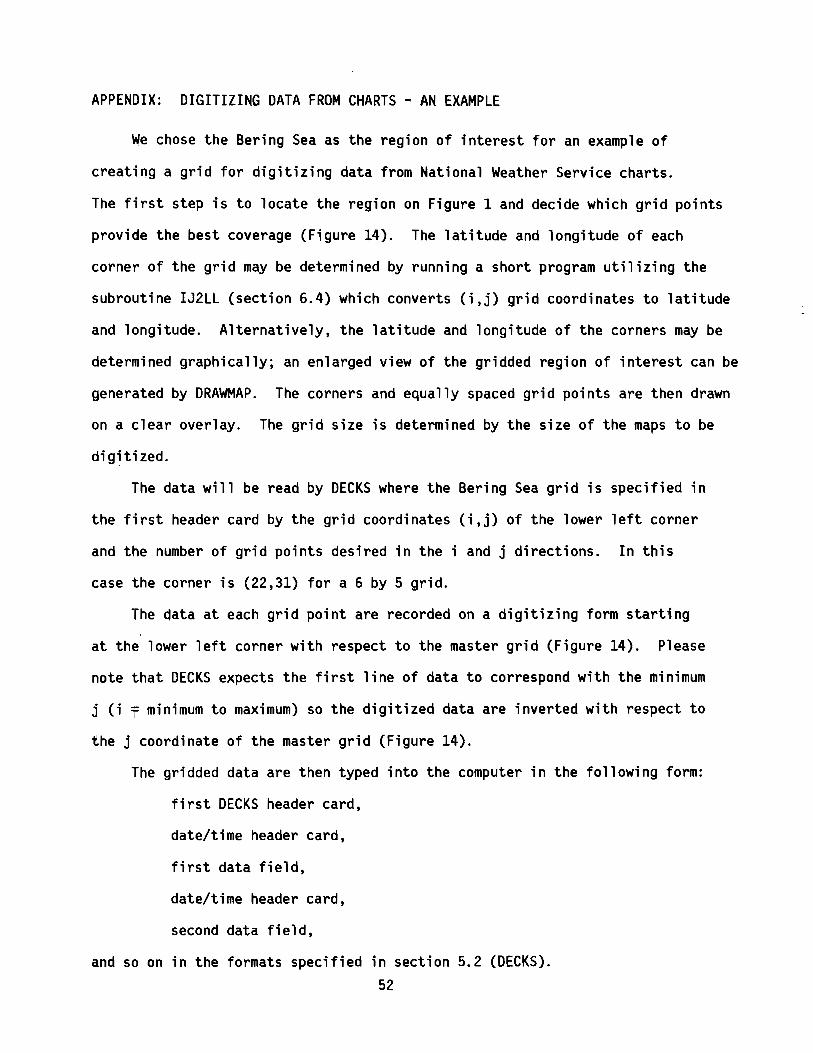
APPENDIX: DIGITIZING DATA FROM CHARTS ~ AN EXAMPLE

We chose the Bering Sea as the region of interest for an example of

creating a grid for digitizing data from National Weather Service charts.

The first step is to locate the region on Figure 1 and decide which grid points

provi~e the best coverage (Figure 14). The latitude and longitude of each

corner of the grid may be determined by running a short program utilizing the

subroutine IJ2LL (section 6.4) which converts (i,j) grid coordinates to latitude

and longitude. Alternatively, the latitude and longitude of the corners may be

determined graphically; an enlarged view of the gridded region of interest can be

generated by DRAWMAP. The corners and equally spaced grid points are then drawn

on a clear overlay. The grid size is determined by the size of the maps to be

digitized.

The data will be read by DECKS where the Bering Sea grid is specified in

the first header card by the grid coordinates (i,j) of the lower left corner

and the number of grid points desired in the i and j directions. In this

case the corner is (22,31) for a 6 by 5 grid.

The data at each grid point are recorded on a digitizing form starting

at the lower left corner with respect to the master grid (Figure 14). Please

note that DECKS expects the first line of data to correspond with the minimum

j (i f minimum to maximum) so the digitized data are inverted with respect to

the j coordinate of the master grid (Figure 14).

The gridded data are then typed into the computer in the following form:

first DECKS header card,

date/time header card,

first data field,

date/time header card,

second data field,

and so on in the formats specified in section 5.2 (DECKS).52

...". "

: .· : . .

. .'.

....". ~ . . . .. . . . ~ . .. .. , ," ..'· . .

j =31'." ",

• • ' • t_

'.

'.." .. .. . ,. .\ .

. . ',".~ .'

." ."

· , . .· . . ..: ."..

'..

. ., .- .

. -. -' J

'"

· .... .

. " ..

i =22

'.,.' .

•22,35 .. 27,35

2~,31, 2"7, 31

1j

(0"

1l~ C"'... .~.J

'\~Lr.......

22,35 27, 3522,31 27,31

GRI D DIGITIZING FORM

Figure 14. To digitize data from charts: locate the grid points that bestcover the area of interest in Fig. I, determine (lat,long) of thecorner grid points, draw a copy of the grid on a clear overlay withsize determined by the chart, record data at each grid point startingwith lower left corner.

53