1

CENTER for SATELLITE APPLICATIONS and

ALGORITHM THEORETICAL BASIS DOCUMENT

ABI Ice Motion

NOAA NESDIS CENTER for SATELLITE APPLICATIONS and

RESEARCH

ALGORITHM THEORETICAL BASIS DOCUMENT

ABI Ice Motion

Yinghui Liu, UW/CIMSS Jeff Key, NOAA/NESDIS/STAR

William Straka III, CIMSS

Version 1.02

September 16, 2010

CENTER for SATELLITE APPLICATIONS and

ALGORITHM THEORETICAL BASIS DOCUMENT

2

TABLE OF CONTENTS 1 Abstract ....................................................................................................................... 6 2 Introduction ................................................................................................................. 6

2.1 Purpose of This Document.................................................................................. 6 2.2 Who Should Use This Document ....................................................................... 6 2.3 Inside Each Section ............................................................................................. 6 2.4 Related Documents ............................................................................................. 7 2.5 Revision History ................................................................................................. 7 2.6 Acknowledgements ............................................................................................. 7

3 Observing System Overview ...................................................................................... 8 3.1 Instrument Characteristics .................................................................................. 8 3.2 Products Generated ............................................................................................. 8 3.3 Instrument Characteristics .................................................................................. 9

4 Algorithm Description .............................................................................................. 10 4.1 Algorithm Overview ......................................................................................... 10 4.2 Processing Outline ............................................................................................ 10 4.3 Algorithm Input ................................................................................................ 12

4.3.1 Primary Sensor Data ................................................................................. 12 4.3.2 Static Ancillary Data ................................................................................. 12

4.3.2.1 Static Ancillary Data ............................................................................. 12 4.3.2.2 Dynamic Ancillary Data ....................................................................... 12

4.4 Theoretical Description ..................................................................................... 12 4.4.1 Ice Motion Physics .................................................................................... 13 4.4.2 Mathematical Description ................................................................. 13 4.4.3 Algorithm Output ................................................................................. 14

5 Test Data Sets and Validations ................................................................................. 17 5.1 Simulated Input Data Sets ................................................................................. 17 5.2 Output from Simulated Inputs Data Sets .......................................................... 18

5.2.1 Precisions and Accuracy Estimates .......................................................... 18 5.2.2 Error Budget.............................................................................................. 19

6 Practical Considerations............................................................................................ 20 6.1 Numerical Computation Considerations ........................................................... 20 6.2 Programming and Procedural Considerations .................................................. 20 6.3 Quality Assessment and Diagnostics ................................................................ 20 6.4 Exception Handling .......................................................................................... 21 6.5 Algorithm Validation ........................................................................................ 21

7 Assumptions and Limitations ................................................................................... 21 7.1 Performance ...................................................................................................... 21 7.2 Assumed Sensor Performance .......................................................................... 21 7.3 Pre-Planned Product Improvements ................................................................. 22

8 References ................................................................................................................. 22

3

LIST OF FIGURES Figure 1. High Level Flowchart of the ice concentration and extent algorithm illustrates the Main Processing Sections. .......................................................................................... 11 Figure 2. Compositie of 11 micron brightness temperature and ice motion vectors from MODIS, using data from Tromso, Norway, for May 20, 2008 ........................................ 18 Figure 3. Compositie of 11 micron brightness temperature and ice motion vectors from MODIS, using data from Tromso, Norway, for May 8, 2008 .......................................... 19 Figure 4. Frequency distributions of ice motion speed (left) and direction (right) difference between MODIS retrieved and from buoy data. .............................................. 20

4

LIST OF TABLES Table 1. Product Function and Performance Specification for sea and lake ice motion. ... 8 Table 2. Summary of the Current ABI Channel Numbers and Wavelengths. ................... 9 Table 3. Sea and Lake Ice Motion Quality Information (3 bytes) ................................... 15 Table 4. Error analysis of retrieved ice motion direction and speed. ............................... 20

5

LIST OF ACRONYMS ABI: Advanced Baseline Imager AIM: ABI Ice Motion AIT: Algorithm Integration Team ATBD: Algorithm Theoretical Basis Document AWG: Algorithm Working Group BT: Brightness Temperature CIMSS: Cooperative Institute for Meteorological Satellite Studies FFT: fast Fourier transforms GOES-R: Geostationary Operational Environmental Satellite R series MODIS: Moderate Resolution Imaging Spectroradiometer MCC: Maximum Cross-Correlation MRD: Mission Requirements Document NH: Northern Hemisphere NIC: National Ice Center NOAA: National Oceanic and Atmospheric Administration SAR: synthetic-aperture-radar USIABP: U.S. Interagency Buoy Program (USIABP)

6

Abstract The cryosphere exists at all latitudes and in about one hundred countries. It has profound socio-economic value due to its role in water resources and its impact on transportation, fisheries, hunting, herding, and agriculture. It also plays a significant role in climate studies, and is critical for accurate weather forecasts. In the cryosphere ice motion is an important property of ice cover. This document provides a high level description of the physical basis and technical approach of an algorithm to retrieve ice motion vectors for ice pixels under clear conditions with supplementary information from observations and products retrieved from the Advanced Baseline Imager (ABI) on the Geostationary Operational Environmental Satellite R series (GOES-R) of the National Oceanic and Atmospheric Administration (NOAA) geostationary meteorological satellites. A Maximum Cross-Correlation procedure is applied to retrieve the ice motion vector. The algorithm is tested using other satellite observations as proxy data for GOES-R ABI. Validations show that the results meet the requirements for product measurement accuracy and precision.

1 Introduction

1.1 Purpose of This Document The ice motion algorithm theoretical basis document (ATBD) provides a high level description of the physical basis for detecting movement of the ice and estimating the speed and direction of ice motion with images from the Advanced Baseline Imager (ABI) flown on the Geostationary Operational Environmental Satellite R series (GOES-R) of the National Oceanic and Atmospheric Administration (NOAA) geostationary meteorological satellites.

1.2 Who Should Use This Document The intended users of this document are those interested in understanding the physical basis and technical implementation of the algorithms, and how to use the output of this algorithm to optimize ice motion for a particular application. This document also provides information useful to anyone implementing, maintaining, and potentially improving the original algorithm.

1.3 Inside Each Section This document is broken down into the following main sections.

• System Overview: Provides relevant details of the ABI and provides a brief description of the products generated by the algorithm.

• Algorithm Description: Provides a detailed description of the algorithm

including its physical basis, its input and its output.

7

• Assumptions and Limitations: Provides an overview of the current limitations of the approach and presents the plan for overcoming these limitations with further algorithm development.

1.4 Related Documents This document currently does not relate to any other document outside of the specifications of the GOES-R Mission Requirements Document (MRD) and to the references given through out.

1.5 Revision History Version 0.2 of this document was created by Yinghui Liu and William Straka III of the Cooperative Institute for Meteorological Satellite Studies (CIMSS), University of Wisconsin-Madison, and Jeffrey Key of NOAA/NESDIS. It is intended to accompany the delivery of the version 0.0 algorithm to the GOES-R Algorithm Working Group (AWG) Algorithm Integration Team (AIT). Version 1.0 was modified by Yinghui Liu and Jeffrey Key for the 80% ready ATBD submitted to AIT.

1.6 Acknowledgements The core ice motion code was provided by Chuck Fowler of the Colorado Center for Astrodynamics Research at the University of Colorado-Boulder. Section 3.4.1 was contributed by Walt Meier of the National Snow and Ice Data Center.

8

Observing System Overview This section describes the products generated by the ABI Ice Motion (AIM) algorithm and the requirements it places on the sensor.

1.7 Instrument Characteristics The ABI onboard the future GOES-R has a wide range of applications in weather, oceanographic, climate, and environmental studies. ABI has 16 spectral bands, with visible bands, 5 near-infrared bands, and 9 infrared bands. The spatial resolution of ABI will be nominally 2 km for the infrared bands, 1 km for the 0.47, 0.86, and 1.61 µm bands, and 0.5 km for the 0.64 µm visible band. ABI will scan the full disk every 15 minutes, plus the continental United States 3 times, plus a selectable 1000 km × 1000 km area every 30 s. ABI can also be programmed to scan the full disk every 5 minutes. Compared to the current GOES imager, ABI offers more spectral bands and higher spatial resolution. In particular, the newly added band at 1.61 µm and higher spatial resolution at 0.64 µm allow for better detection and monitoring of surface snow and ice (Schmit et al., 2005).

1.8 Products Generated The ice motion algorithm is responsible for determining the motion of ice pixels for all clear and non-land ABI pixels with sea ice cover. In terms of the MRD, it is responsible directly for the movement within the Cryosphere category. The current ice motion design calls for a u and v movement in pixel space. The required product Function and Performance Specification (F&PS) for ice motion is listed in Table 1.

Table 1. Product Function and Performance Specification for sea and lake ice motion.

Name Sea & Lake Ice motion Sea & Lake Ice Motion User and Priority GOES-R GOES-R Geographic Coverage (G, H, C, M) C: Great Lakes and

Chesapeake and Delaware Bays only

FD: Sea ice covered waters in N & S Hemisphere

Vertical Resolution N/A N/A Horizontal Resolution 5 km 15 km Mapping Accuracy 2.5 km 7.5 km Measurement Range Direction: 0 to 360°,

and displacement 0 to 0.6 m/s

Direction: 0 to 360°, and displacement 0 to 0.6 m/s

Measurement Accuracy Direction: 22.5°, Speed 3 km/day

Direction: 22.5°, Speed 3 km/day

Product Refresh Rate/Coverage Time 3 hr 6 hr Vendor Allocated Ground 3236 sec 9716 sec Product Measurement Precision Direction: 30°, Speed 3 Direction: 30°, Speed 3

9

km/day km/day

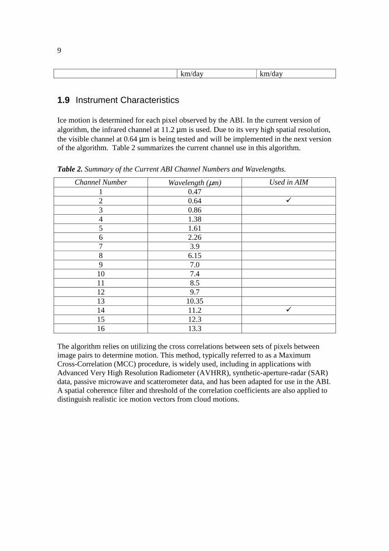
1.9 Instrument Characteristics Ice motion is determined for each pixel observed by the ABI. In the current version of algorithm, the infrared channel at 11.2 µm is used. Due to its very high spatial resolution, the visible channel at 0.64 µm is being tested and will be implemented in the next version of the algorithm. Table 2 summarizes the current channel use in this algorithm.

Table 2. Summary of the Current ABI Channel Numbers and Wavelengths.

Channel Number Wavelength (µm) Used in AIM 1 0.47 2 0.64 � 3 0.86 4 1.38 5 1.61 6 2.26 7 3.9 8 6.15 9 7.0 10 7.4 11 8.5 12 9.7 13 10.35 14 11.2 � 15 12.3 16 13.3

The algorithm relies on utilizing the cross correlations between sets of pixels between image pairs to determine motion. This method, typically referred to as a Maximum Cross-Correlation (MCC) procedure, is widely used, including in applications with Advanced Very High Resolution Radiometer (AVHRR), synthetic-aperture-radar (SAR) data, passive microwave and scatterometer data, and has been adapted for use in the ABI. A spatial coherence filter and threshold of the correlation coefficients are also applied to distinguish realistic ice motion vectors from cloud motions.

10

Algorithm Description A complete description of the algorithm at its current level of maturity (which will improve with each revision) is provided in this section. An overview, processing outline and a more in depth description of the basis for the algorithm are included.

1.10 Algorithm Overview The ABI ice motion algorithm is based upon the methodology used by the National Snow and Ice Data Center’s Polar Pathfinder Daily 25 km EASE-Grid Sea Ice Motion Vectors for gathering ice motion vectors from the AVHRR instrument and passive microwave observations (Fowler 2003). The ice motion output is in x and y coordinates of a standardized global grid, with the u and v components of motion.

1.11 Processing Outline The processing outline of the AIM is summarized as follows:

- Process full image of 11-micron channel data in Brightness Temperature (BT) - Load 11-micron image from 24 hours prior. Re-map both 11-micron images to

common grid. - Make common cloud mask containing current and cloud mask from 24 hours

prior and re-map to common grid - Run motion executable - Run vector filtering executable

o This outputs vectors of points and motion in pixel space A flow chart of the processing of the AIM is shown below.

Ice motion algorithm begin

Current and 24-hour previous ABI channel BTs and cloud mask,

land/water mask

ABI Channel Used: Channel No 14. Algorithm Dependencies: Cloud mask Ice mask Ancillary Data Dependencies: Land/water mask. Products Generated: Ice motion vector and associated quality flags.

Re-map BTs to common grid

Calculate Maximum cross-correlation

11

Figure 1. High Level Flowchart of the ice concentration and extent algorithm illustrates the Main Processing Sections.

12

1.12 Algorithm Input This section describes the input needed to process the AIM. The AIM requires knowledge of the surrounding pixels. In its current operation, we run the AIM on all pixels from both the current and previous images. The AIM is not designed to run with information from only one pixel or just one image.

1.12.1 Primary Sensor Data The list below notes the primary sensor data used by the AIM. By primary sensor data, we mean information that is derived solely from the ABI observations and geo-location information.

• Current calibrated brightness temperatures for the 11-micron channel • Calibrated 11-micron channel brightness temperatures from 24 hours previous.

1.12.2 Ancillary Data

1.12.2.1 Static Ancillary Data Static ancillary data represent data that require information not included in the ABI observations or geo-location data and do not change with each image. The only static dataset that is useful to the AIM is the pixel level land/water mask. This data set can be an output from the AIT Framework data structures.

1.12.2.2 Dynamic Ancillary Data Dynamic ancillary data represent data that change with each image and are not included in the ABI observations or geo-location data. The AIM requires two sets of dynamic ancillary data. First are the current image pixel level cloud and ice masks, and second are the cloud and ice masks from the image 24 hours previous. These data are necessary to accurately determine where clear sky and ice pixels are located.

1.13 Theoretical Description Ice motion detection is the process of determining the movement of pixels that are ice pixels. It always involves assumptions of the radiometric characteristics of ice, particularly those that relate to the brightness temperature in the 11-micron channel. In the AIM, a small target area in one image is correlated with many areas of the same size in a search region of the second image. The displacement of the ice is then defined by the location in the second image where the correlation coefficient is the highest with the small target area in the first image. This process makes the basic assumptions that the sea-ice cover can be treated as a solid, with the ice movement only a translation of this

13

solid plane (e.g., ignoring deformation and rotation of the ice), and the radiative property of the pixels does not change significantly over the 24 hour period. These assumptions are generally valid over short distances and away from ice edges such as the marginal ice zone where the ice is less constrained. However, radiative properties can change during onset of melt, snowfall, etc. (Maslanik et al., 1998). Furthermore, two extra filterings are applied to the output ice motion vectors as described later to get better results. Selecting the sizes of the target area and search windows in the images depends upon several factors. The size of the target window cannot be so large as to negate this solid-plane assumption, but the window size must be large enough so that the correlation still has some statistical significance. Also, the size of the search window is dependent on the expected displacement of the ice. For small areas of movement (such as the Great Lakes), this window must be less than a few pixels. In the current algorithm, a 15 pixel by 15 pixel search window is selected. The size and shape of the search window is being tested, and can be changed in the next version of algorithm.

1.13.1 Ice Motion Physics The motion of an individual ice floe is governed by the balance of the forces that act on that floe. This relationship can be expressed using what is often called the momentum equation, simply Newton’s third law of motion:

∑ ==Dt

DummaF

where m is the mass of the ice. We usually express the forces in terms of stress (force per unit area), so the mass will be in mass per unit area, or the ice density multiplies by its thickness (H). The external stresses acting on the ice floe are the wind stress, τa, the water stress, τw, the apparent force due to Coriolis, τc, the force due the tilt of the water surface, τt, and the internal ice stress, τi. Therefore,

itcwaDt

Dum τττττ ++++=

Which terms are most important depends on the scales of interest. More details can be found in Maslanik et al. (1998) and Thorndike and Colony (1982). Theoretically, the ice motion vector can be derived by solving the above non-linear equation. In satellite remote sensing applications, correlation coefficient analysis between two satellite images is often used to derive ice motion vectors. Details are explained in the next section.

1.13.2 Mathematical Description

14

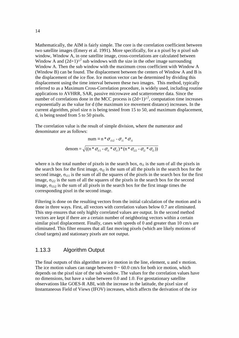
Mathematically, the AIM is fairly simple. The core is the correlation coefficient between two satellite images (Emery et al. 1991). More specifically, for a n pixel by n pixel sub window, Window A, in one satellite image, cross-correlations are calculated between Window A and (2d+1)^2 sub windows with the size in the other image surrounding Window A. Then the sub window with the maximum cross coefficient with Window A (Window B) can be found. The displacement between the centers of Window A and B is the displacement of the ice floe. Ice motion vector can be determined by dividing this displacement using the time interval between these two images. This method, typically referred to as a Maximum Cross-Correlation procedure, is widely used, including routine applications to AVHRR, SAR, passive microwave and scatterometer data. Since the number of correlations done in the MCC process is (2d+1)^2, computation time increases exponentially as the value for d (the maximum ice movement distance) increases. In the current algorithm, pixel size n is being tested from 15 to 50, and maximum displacement, d, is being tested from 5 to 50 pixels. The correlation value is the result of simple division, where the numerator and denominator are as follows: where n is the total number of pixels in the search box, σi1 is the sum of all the pixels in the search box for the first image, σi2 is the sum of all the pixels in the search box for the second image, σi11 is the sum of all the squares of the pixels in the search box for the first image, σi22 is the sum of all the squares of the pixels in the search box for the second image, σi1i2 is the sum of all pixels in the search box for the first image times the corresponding pixel in the second image. Filtering is done on the resulting vectors from the initial calculation of the motion and is done in three ways. First, all vectors with correlation values below 0.7 are eliminated. This step ensures that only highly correlated values are output. In the second method vectors are kept if there are a certain number of neighboring vectors within a certain similar pixel displacement. Finally, cases with speeds of 0 and greater than 10 cm/s are eliminated. This filter ensures that all fast moving pixels (which are likely motions of cloud targets) and stationary pixels are not output.

1.13.3 Algorithm Output The final outputs of this algorithm are ice motion in the line, element, u and v motion. The ice motion values can range between 0 ~ 60.0 cm/s for both ice motion, which depends on the pixel size of the sub window. The values for the correlation values have no dimensions, but have a value between 0.0 and 1.0. For geostationary satellite observations like GOES-R ABI, with the increase in the latitude, the pixel size of Instantaneous Field of Views (IFOV) increases, which affects the derivation of the ice

i1i1i1i2 *-*n num σσσ=

))*-*(n*)*-*((n = denom i2i2i22i1i1i11 σσσσσσ

15

motion vectors and their qualities, e.g. resolution. The maximum latitude of the ice motion vector is the latitude with a 67 degree local zenith angle, which corresponds to latitudes less than 60 degrees. For a pixel size of 2 km under the nadir view, the resolution near the Arctic, 60 degree North, is around 5 km, and the resolution over the Great Lakes, 45 degree North, is around 3 km. With better image resolution for the visible channel, 0.5 km at the 0.64 µm channel, the image resolution is around 0.75 km over the Great Lakes and 1.25 km over 60 degree North latitude, which improves the quality of the ice motion vectors. In this regard, observations with higher spatial resolution, like 0.5 km spatial resolution for ABI’s 0.64 µm channel, will improve the quality of the output ice motion vector. The quality flag information of the product is listed in Table 3, with metadata information followed.

Table 3. Sea and Lake Ice Motion Quality Information (3 bytes)

Byte Bit Quality Flag Name Description Meaning

0

0 QC_INPUT_PREV Valid input from previous image 0-yes 1-no 1 QC_INPUT_NOW Valid input from current image 0-yes 1-no

2 QC_CLDMASK_PREV Valid cloud mask from previous

image 0-yes 1-no

3 QC_CLDMASK_NOW Valid cloud mask from current

image 0-yes 1-no

4 QC_ICEMASK_PREV Valid ice cover from previous

image 0-yes 1-no

5 QC_ICEMASK_PREV Valid ice mask from current

image 0-yes 1-no

6

QC_INPUT_SURFACE Surface background flag

00 - in-land water 01 - sea water

10- land 11 - others

7

2

0 QC_VALID_PIXEL_NOW

Percentage of pixels over water surface under clear conditions in a sub-window in current image is

greater than set threshold

0-yes 1-no

1 QC_VALID_PIXEL_PREV

Percentage of pixels over water surface under clear conditions in

sub-windows in previous image is greater than set threshold

0-yes 1-no

2 QC_VALID_CORR Maximum correlation coefficient

is larger than the set threshold 0-yes 1-no

3 QC_VALID_SRFC_NOW Surface is ice covered in the sub-

window in current image 0-yes 1-no

4 QC_VALID_SRFC_PREV Surface is ice covered in the sub-

window in previous image 0-yes 1-no

5 QC_FILTER Pass the filtering 0-yes 1-no 6 7

3 0 QC_INPUT_LOCALZEN

Local zenith angle is less than set threshold (67 degree)

0-yes 1-no

1 QC_DERIVED_U u-component is less than set 0-yes 1-no

16

threshold

2 QC_DERIVED_V u-component is less than set

threshold 0-yes 1-no

3 4 5 6 7

Sea and Lake Ice Motion File Metadata: Common metadata for all data products:

� DateTime (swath beginning and swath end) � Bounding Box

• Product resolution (nominal and/or at nadir) • Number of rows, and number of columns • Bytes per pixel • Data type • Byte order information • Location of box relative to nadir (pixel space)

� Product Name � Product units � Ancillary data to produce product (including product precedence and interval

between datasets is applicable) • Version Number • Origin • Name

� Satellite � Instrument � Altitude � Nadir pixel in the fixed grid � Attitude � Latitude, longitude � Grid projection � Type of scan � Product version number � Data compression type � Location of production � Citations to documents � Contact information

Sea and Lake Ice Motion Specific Metadata:

� Pixel size of sub-window � Maximum Local zenith angle limit � Threshold of minimum clear-sky water surface percentage in a sub-window

17

� Maximum correlation coefficient threshold � Threshold of maximum u and v-component � Total number of pixels with ice cover � Total number of valid ice motion retrievals � Total percentage of valid ice motion retrievals of all pixels with ice cover � Total pixel numbers and percentage of terminator pixels (Non-retrievable and Bad

data) � Mean, Min, Max, and standard deviation of the speed of the ice motion retrievals � Mean, Min, Max, and standard deviation of the direction of the ice motion

retrievals

2 Test Data Sets and Validations

2.1 Simulated Input Data Sets Currently the AIM is being simulated and tested in near real time at the Moderate Resolution Imaging Spectroradiometer (MODIS) Direct Broadcast site at Tromsø, Norway, using data from the Integrated Program Office's direct broadcast system, operated by Kongsberg Satellite Services (Ksat). This data is then compared to buoy measurements from the International Arctic Buoy Program, operated by the University of Washington, with funding from the U.S. Interagency Buoy Program (USIABP) through the National Ice Center (NIC). MODIS is used because of its coverage over the regions with buoy measurements as well as coverage of moving ice on a nearly daily basis. Further validation over the mid-latitudes will be carried out when in situ observations become available. The direct broadcast system is useful as it provides a platform for near-realtime processing testing. Data is remapped to a standard grid, much like what is proposed for ABI. In addition, the location of the direct broadcast systems in the polar regions allows for near complete coverage of the Arctic and Antarctic testing in near real time.

18

Figure 2. Compositie of 11 micron brightness temperature and ice motion vectors from MODIS, using data from Tromso, Norway, for May 20, 2008.

2.2 Output from Simulated Inputs Data Sets

2.2.1 Precisions and Accuracy Estimates A test case study was taken from May 4-9, 2008, utilizing near realtime data from the MODIS Direct Broadcast site at Tromsø, Norway, operated by Ksat. Buoy measurements provide latitude, longitude and UTC every 45 minutes to 1 hour. Using these observations, we can calculate speed and direction of the buoy. Evaluation of the buoy data and data measured from the AIM was performed by assuming that motion is within 50km of the buoy data. Consequently, there are a total of 50 comparisons for this time period (see an example in Figure 3).

19

Figure 3. Compositie of 11 micron brightness temperature and ice motion vectors from MODIS, using data from Tromso, Norway, for May 8, 2008.

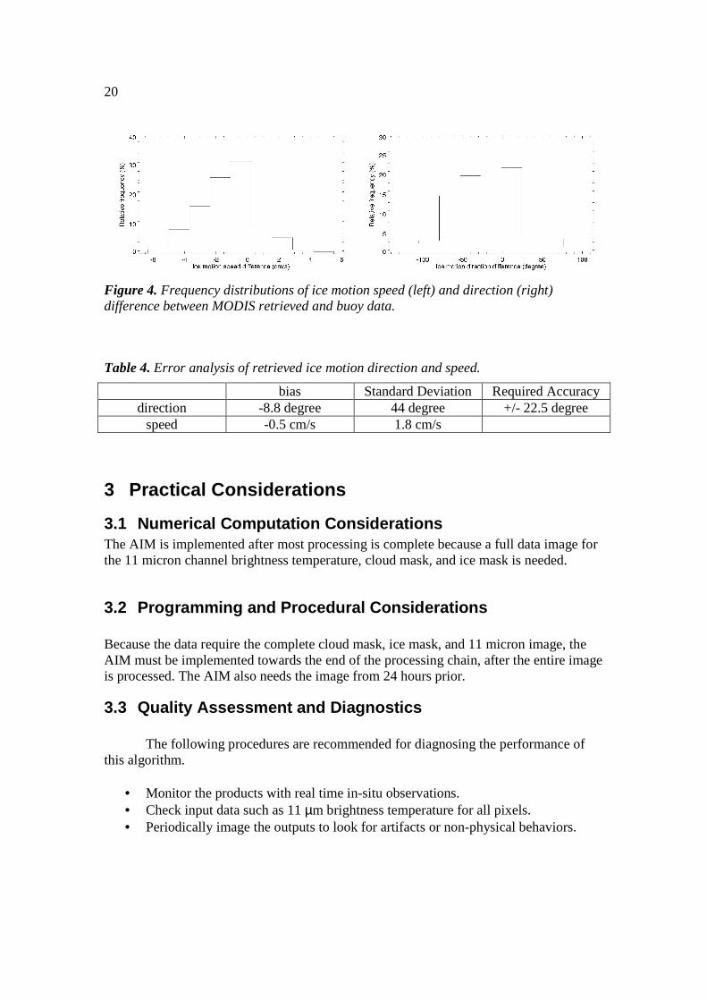
2.2.2 Error Budget The average speed difference for the case study time period was approximately –0.5 cm/s with a standard deviation of 1.8 cm/s. The average directional difference was –8.8 degrees. The maximum speed difference was around 6 cm/s, and the maximum absolute directional difference was around 50 degrees (Figure 4, Table 4). These large differences are likely due to the fact that none of the ice motion vectors were closer than about 20 km. Based on this case, the accuracy of this algorithm meets the MRD requirement. However, more cases and extensive validations need be carried out, including more cases over the Arctic, and over the Great Lakes regions.

20

Figure 4. Frequency distributions of ice motion speed (left) and direction (right) difference between MODIS retrieved and buoy data.

Table 4. Error analysis of retrieved ice motion direction and speed.

bias Standard Deviation Required Accuracy direction -8.8 degree 44 degree +/- 22.5 degree

speed -0.5 cm/s 1.8 cm/s

3 Practical Considerations

3.1 Numerical Computation Considerations The AIM is implemented after most processing is complete because a full data image for the 11 micron channel brightness temperature, cloud mask, and ice mask is needed.

3.2 Programming and Procedural Considerations Because the data require the complete cloud mask, ice mask, and 11 micron image, the AIM must be implemented towards the end of the processing chain, after the entire image is processed. The AIM also needs the image from 24 hours prior.

3.3 Quality Assessment and Diagnostics The following procedures are recommended for diagnosing the performance of this algorithm.

• Monitor the products with real time in-situ observations. • Check input data such as 11 µm brightness temperature for all pixels. • Periodically image the outputs to look for artifacts or non-physical behaviors.

21

3.4 Exception Handling This algorithm checks the validity of input data before running, as well as checks for missing input variables values.

3.5 Algorithm Validation The current validation cases are limited. More extensive validation will be carried out using proxy data, such as MODIS, and other proxy data sets, over ocean and the Great Lakes, in comparison with ice motion products from buoy observations, ice charts, and other resources.

4 Assumptions and Limitations The following sections describe the current limitations and assumptions in the current version of the AIM.

4.1 Performance The following assumptions have been made in developing and estimating the performance of the AIM.

1. The cloud mask provides an accurate clear sky mask for both the current and scene 24 hours prior in a timely manner.

2. Land mask maps are available to identify land/water pixels and are available at the pixel level.

3. Sensor data for the 11 micron channel are available for the current and scene 24 hours prior in a timely manner.

4. All data are in the same gridded format and in the same orientation.

4.2 Assumed Sensor Performance We assume the sensor will meet its current specifications. However, the AIM will be dependent on the following instrument characteristics:

• The cross correlation of each search bin in the AIM will be critically dependent on the amount of striping in the data.

• Unknown spectral shifts in some channels will cause biases in calculating the cross-correlations and may impact the performance of the AIM.

• The AIM is critically dependent on the quality of the cloud mask, ice mask, as well as 11 micron sensor data.

• Errors in navigation from image to image will affect the re-mapping of the data into pixel space.

22

• All sensor issues can play a role in accurate clear sky detection. In addition, it is assumed that the cloud mask is an accurate portrayal of clear/cloudy pixels.

4.3 Pre-Planned Product Improvements To improve its accuracy before satellite launch, this algorithm will continue to be modified. In-depth research will be carried out during the process. Below are some areas currently being investigated:

• Size of the sub-window will be tested to get the best results. The current size of the search window is 15 pixels by pixels.

• The shape of the sub-window (square versus circle) will be tested to get the best results. The current shape of the sub-window is 15 pixel by pixel square. The lake ice near shore has an irregular shape, which should be taken into consideration

• The instrument noise on the final retrieval results is being investigated. • Different re-map plans will be applied to pick the best map projection.

5 References Emery, W.J., C.W. Fowler, J. Hawkins, and R.H. Preller, 1991. Fram Strait satellite image derived ice motions, J. Geophys. Res., 96, 4751-4768. Fowler, C. 2003, updated 2007. Polar Pathfinder Daily 25 km EASE-Grid Sea Ice Motion Vectors. Boulder, Colorado USA: National Snow and Ice Data Center. Digital media. Maslanik, J., C. Fowler, J. Key, T. Scambos, T. Hutchinson, and W. Emery. 1998. AVHRR-based Polar Pathfinder products for modeling applications. Annals of Glaciology 25:388-392. Schmit, Timothy J., Mathew M. Gunshor, W. Paul Menzel, James J. Gurka, Jun Li, A. Scott Bachmeier, 2005: INTRODUCING THE NEXT-GENERATION ADVANCED BASELINE IMAGER ON GOES-R. Bull. Amer. Meteor. Soc., 86, 1079-1096 Thorndike, A. S., and R. Colony (1982), Sea Ice Motion in Response to Geostrophic Winds, J. Geophys. Res., 87(C8), 5845\u20135852, doi:10.1029/JC087iC08p05845.