Noname manuscript No.(will be inserted by the editor)

NMR Assignment through Linear Programming

Jose F. S. Bravo-Ferreira · DavidCowburn · Yuehaw Khoo · Amit Singer

Received: date / Accepted: date

Abstract Nuclear Magnetic Resonance (NMR) Spectroscopy is the second mostused technique (after X-ray crystallography) for structural determination of pro-teins. A computational challenge in this technique involves solving a discrete opti-mization problem that assigns the resonance frequency to each atom in the protein.This paper introduces LIAN (LInear programming Assignment for NMR), a novellinear programming formulation of the problem which yields state-of-the-art re-sults in simulated and experimental datasets.

Keywords NMR spectroscopy · Shortest path problem · Resonance assignmentproblem · Linear programming relaxation

1 Introduction

We investigate a type of constraint satisfaction problem on certain graphs arising inNMR Spectroscopy. Crucial to NMR spectroscopy is the time-consuming chemicalshift assignment problem (also known as the spectral or resonance assignmentproblem) [14], which inhibits the wider application of this technique. To date,this procedure is done largely in a semi-manual way, even though approachesusing exhaustive search [25], integer programming [2], genetic algorithms [29],

Jose F. S. Bravo-FerreiraPACM, Princeton University, NJ 08540E-mail: josesf@princeton.edu

David CowburnDepartments of Biochemistry and of Physiology and Biophysics, Albert Einstein College ofMedicine, NY 10461E-mail: cowburn@cowburnlab.org

Yuehaw KhooDepartment of Statistics, University of Chicago, IL 60637E-mail: ykhoo@uchicago.edu

Amit SingerDepartment of Mathematics and PACM, Princeton University, NJ 08540E-mail: amits@math.princeton.edu

arX

iv:2

008.

0364

1v2

[cs

.AI]

8 S

ep 2

021

2 Jose F. S. Bravo-Ferreira et al.

variants of belief propagation [4], among others, have all shown promise in differentexperimental datasets. However, these approaches typically lack either a principleddefinition of the cost function, or a way to determine whether the global optimizeris every attained. In this paper, we attempt to address these issues in the searchfor a more rigorous algorithm.

1.1 The assignment problem

The spectral assignment problem is the problem of determining the resonancefrequencies of individual atoms in the protein. These frequencies are typicallydefined by their chemical shifts, measured in parts per million (ppm) relative toa reference compound since they depend on the local environment of individualnuclei [12]. Therefore, the resonance frequencies are often referred to as chemicalshifts.

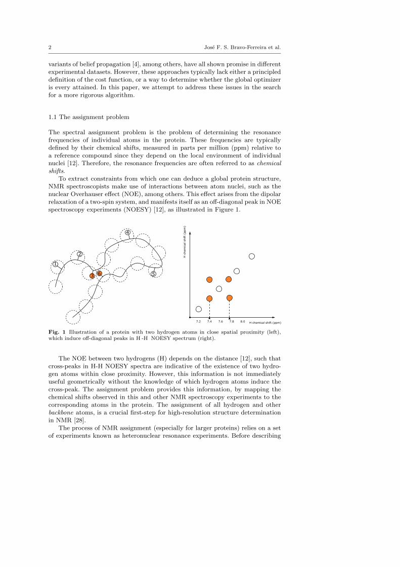
To extract constraints from which one can deduce a global protein structure,NMR spectroscopists make use of interactions between atom nuclei, such as thenuclear Overhauser effect (NOE), among others. This effect arises from the dipolarrelaxation of a two-spin system, and manifests itself as an off-diagonal peak in NOEspectroscopy experiments (NOESY) [12], as illustrated in Figure 1.

Fig. 1 Illustration of a protein with two hydrogen atoms in close spatial proximity (left),which induce off-diagonal peaks in H -H NOESY spectrum (right).

The NOE between two hydrogens (H) depends on the distance [12], such thatcross-peaks in H-H NOESY spectra are indicative of the existence of two hydro-gen atoms within close proximity. However, this information is not immediatelyuseful geometrically without the knowledge of which hydrogen atoms induce thecross-peak. The assignment problem provides this information, by mapping thechemical shifts observed in this and other NMR spectroscopy experiments to thecorresponding atoms in the protein. The assignment of all hydrogen and otherbackbone atoms, is a crucial first-step for high-resolution structure determinationin NMR [28].

The process of NMR assignment (especially for larger proteins) relies on a setof experiments known as heteronuclear resonance experiments. Before describing

NMR Assignment through Linear Programming 3

(a1, a2, a4)

(a1, a2, a3)

p1

p2 p3p5p6

p4

pi ∈ ℝ3

Fig. 2 Representing the assignment problem as a graph. Each node is associated with a tripletof atoms (e.g. (a1, a2, a3) or (a1, a2, a4)). When two triplets share some atoms, there is an edgejoining them. Each triplet gives rise to a resonance peak in the 3-dimensional spectra. The goalis to assign the measured peaks to the nodes or triplets. Crucially, when two peaks result fromtwo triplets that share some common atoms, they will share certain coordinates. For example,(a1, a2, a3) and (a1, a2, a4) share (a1, a2), so the coordinates in the horizontal plane of theresulting peaks p1, p3 are the same (indicated by the vertical dotted line).

these experiments in detail, we first provide some background information on pro-tein structure. A protein is composed of a chain of residues. Every residue containsthe same set of atoms HN , N, Cα, Cβ (with the exception of Proline). These re-peated elements then form the protein backbone. Basic heteronuclear experimentscouple (HN , N), (HN , N, Cα), or (HN , N, Cβ) from a single residue or two adja-cent residues. Ideally, these pairs or triplets contribute to the resonance peaks ona 2- or n-dimensional spectra, where the coordinates of the peak are the resonancefrequencies of the hydrogen, nitrogen and carbon (similar to the case in Figure 1).As different triplets (or pairs) may share common atoms, this results in a graphsuch as the one depicted in Figure 2, where a node resembles a triplet (pair), andan edge between two nodes means two triplets (pairs) share one or two atoms.The goal of the assignment procedure is to take the measured peaks in R3 (peaksin R2 resulted from (N, HN ) can be embedded into R3), and assign them to theappropriate nodes in the graph. An edge between two nodes induces a constraintthat the two assigned peaks must share coordinates across certain dimensions.

In the next subsection, we describe different kinds of measurements one can per-form to couple different pairs or triplets, giving rise to peaks in 2- or 3-dimensionalspectra that facilitate the assignment procedure. Readers unfamiliar with thechemistry involved may skip the rest of the next subsection, and read Section 2where we elucidate the general philosophy of how these spectra can be used ingraph theoretic notions.

1.2 Typical spectra used for assignment

In this section we detail three basic experiments which are commonly used forbackbone assignment of small proteins (<150 residues). As we shall see, these

4 Jose F. S. Bravo-Ferreira et al.

three sets of experiments can provide an assignment of the peaks. They give riseto the three types of spectra detailed below.

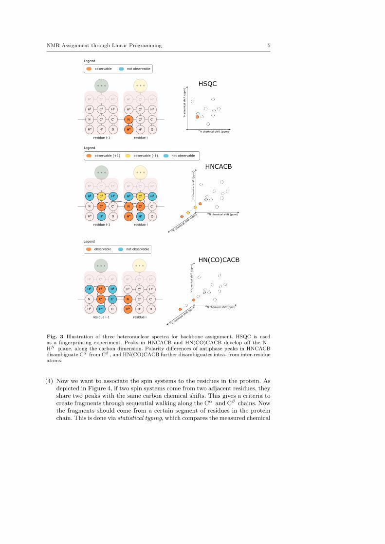
HSQC The heteronuclear single quantum coherence experiment [10] involves atransfer of magnetization between the base amide proton, HN , and the nitrogenN and back, as illustrated in Figure 3. With the exception of proline, all basicamino acids feature this amide pair, such that a distinct peak can be expected formost residues, leading to the use of HSQC as a fingerprinting experiment.

HNCACB This experiment involves magnetization transfer from Hα and Hβ toCα and Cβ , respectively, and then from Cβ to Cα and finally to N and to HN

of the same or subsequent residue, as illustrated in Figure 3, and described in[18]. The polarities of the Cα and Cβ peaks are opposite, which allows theseto be distinguished. Importantly, note that Cα and Cβ peaks are observed withthe same root N –HN pair. This means there should be four peaks in HNCACBspectra, having the same frequency in the N and HN dimension. This allows forsequential walking (Section 1.2.1), the process of matching residues with theirneighbors through matching carbon frequencies.

HN(CO)CACB The last of the experimental toolset for backbone assignment ofmedium-size proteins also gives rise to Cα and Cβ peaks [17], as illustrated inFigure 3. Magnetization transfer happens from Hα and Hβ to Cα and Cβ , ontoCO' and finally the base amide pair. Chemical shifts are evolved only on Cα andCβ before detection, so no CO' peaks are observed.

1.2.1 Basic assignment procedure

Given this set of experiments, a greedy way of assignment (Figure 4) is summarizedin this section. This procedure forms the backbone of many assignment algorithms.It is as follows:

(1) HSQC is used as a fingerprint experiment due to high sensitivity and resolution,allowing for accurate determination of base N –HN pairs. As we can see inFigure 4, peaks in HNCACB and HN(CO)CACB can be grouped accordingto frequency in the N and HN . Therefore, peaks in HSQC are matched withpeaks in HNCACB and HN(CO)CACB spectra which satisfy tolerance bounds(typically 0.02 - 0.03 ppm for hydrogen and 0.20 - 0.30 ppm for nitrogen).

(2) After grouping the peaks in HNCACB and HN(CO)CACB, within the same N –HN grouping, the peaks are further correlated and disambiguated using phaseinformation, allowing for the assembly of spin systems. Firstly, HN(CO)CACBtells which of the four peaks in HNCACB comes from the carbons of previousresidue, while the +/- sign in HNCACB distinguishes Cα from Cβ .

(3) After steps (1) and (2), peaks from HSQC, HN(CO)CACB, HNCACB arecombined, resulting in groups of peaks where each group has four peaks. Eachgroup is called a spin system. We re-emphasize that the peaks within the samespin system have the same N and HN frequency, but the frequency along thecarbon axis differs. There should be as many spin systems as the number ofresidues (with a few exceptions), since each residue has exactly one pair ofN –HN .

NMR Assignment through Linear Programming 5

HN Hα

N Cα

Hβ Cβ

Hγ Cγ

O

C'

Hβ

Hγ

HN Hα

N Cα

Hβ Cβ

Hγ Cγ

O

C'

Hβ

Hγ

residue i-1 residue i

... ...

observable not observable

Legend

15N chemical shift (ppm)

1H

chem

ical

shift

(ppm

)

HN

N

HSQC

HN Hα

N Cα

Hβ Cβ

Hγ Cγ

O

C'

Hβ

Hγ

HN Hα

N Cα

Hβ Cβ

Hγ Cγ

O

C'

Hβ

Hγ

residue i-1 residue i

... ...

observable (+1) not observable

Legend

observable (-1)

15N chemical shift (ppm)

1H

chem

ical

shift

(ppm

)

13 C chem

ical s

hift (

ppm)

HN

N

HNCACB

Hα

Cα

Hβ Cβ Hβ

Hα

Cα

Hβ Cβ Hβ

HN Hα

N Cα

Hβ Cβ

Hγ Cγ

O

C'

Hβ

Hγ

HN Hα

N Cα

Hβ Cβ

Hγ Cγ

O

C'

Hβ

Hγ

residue i-1 residue i

... ...

observable not observable

Legend

15N chemical shift (ppm)

1H

chem

ical

shift

(ppm

)

13 C chem

ical s

hift (

ppm)

HN

N

HN(CO)CACB

Hα

Cα

Hβ Cβ Hβ

C'

Fig. 3 Illustration of three heteronuclear spectra for backbone assignment. HSQC is usedas a fingerprinting experiment. Peaks in HNCACB and HN(CO)CACB develop off the N –HN plane, along the carbon dimension. Polarity differences of antiphase peaks in HNCACBdisambiguate Cα from Cβ , and HN(CO)CACB further disambiguates intra- from inter-residueatoms.

(4) Now we want to associate the spin systems to the residues in the protein. Asdepicted in Figure 4, if two spin systems come from two adjacent residues, theyshare two peaks with the same carbon chemical shifts. This gives a criteria tocreate fragments through sequential walking along the Cα and Cβ chains. Nowthe fragments should come from a certain segment of residues in the proteinchain. This is done via statistical typing, which compares the measured chemical

6 Jose F. S. Bravo-Ferreira et al.

shifts of atoms in the identified fragments with the expected chemical shift ofthe residues collected in a public database such as BMRB [30]. The fragmentsare placed optimally according to that prior.

We remark that that the widespread availability of NMR data collected indatabases such as BMRB is fundamental in assignment. The distributions of chem-ical shifts in different amino acid types is not the same, due to the unique environ-ment induced by the different chemical structures. Certain amino acids, includingalanine, glycine, isoleucine, leucine, proline, serine, threonine, and valine, presentparticularly distinct signatures. Among these, Glycine and Proline are unique inthat they do not feature certain peaks. Specifically, Glycine is characterized by itsunique Cα shift and the absence of a Cβ signal (see, e.g. [19]). Proline, as theonly secondary amine among proteinogenic amino acids, does not yield peaks inthe experiments described above. As a result, such residues are only identified asneighbors through HN(CO)CACB spectra or via specific experiments (e.g. [26]).

We also note, however, that the local chemical environment can shift the reso-nance frequencies of certain atoms, even if they belong to the same residue type.In fact, local chemical shifts can be used as predictors for the chemical shift ofa specific atom (see, e.g., [34]), which means that sophisticated probabilistic de-scriptions of the resonance frequencies may be necessary for certain proteins, orthat an iterative process taking into account the primary and secondary structureof the protein should be employed.

1.2.2 Challenges in sequential assignment

As described above, accurate assignment relies on the correct identification ofpeaks in NMR experiments, and their assembly into consistent spin systems thatcan be sequentially assigned.

In practice, as the quality of NMR spectra deteriorates, some peaks will over-lap, and others cannot be detected at all, due to peak broadening and lower SNR.Artifacts included in automatically selected peak lists further hamper sequentialassignment. Even with a decent set of spin systems, sequential assignment itself isnot as simple as solving a one-dimensional puzzle, as experimental noise, erroneousspin systems, overlapping chemical shifts, and missing spin systems introduce am-biguity to the process.

1.3 Our contributions

The contribution of the paper is two-fold:

1. We formulate the spectral assignment problem as a constraint satisfaction prob-lem, with cost being defined on a graph G = (V,E):

min{zi}i∈V⊂{0,1}m

∑(i,j)∈E

fij(zi, zj), s.t. linear constraints on z1, . . . , z|V |. (1)

Here zi’s are indicator vectors associated with nodes V .

NMR Assignment through Linear Programming 7

15N

1H

HSQC

15N

1H

13 C

HN(CO)CACB

15N

1H

13 C

HNCACB

1 2

34

HN(CO)CACBHNCACB

Cα

Cα

Cβ

Cβ

Ci-1

?

?

?

? Ci-1?

?

Spin Systems

... ...N G K T L K G E T T T E A

Fig. 4 Sketch of backbone assignment procedure through heteronuclear NMR. (1) HSQCpeaks are used as fingerprints and linked to matching peaks in HN(CO)CACB and HNCACBspectra. (2) The carbon dimension in HNCACB and HN(CO)CACB is used along with phaseinformation to identify specific atom frequencies. (3) Spin systems are created from thesefragments, each containing carbon frequencies for two adjacent residues. (4) Spin systems areordered into fragments (based on matching carbon frequencies) and placed in their correctposition through statistical typing (using prior information from a public database of chemicalshift statistics).

2. In general, this type of problem is hard to solve, unless G is tree-like. However,the adjacency matrix of graph G in the assignment problem forms a bandmatrix, which allows us to reformulate (1) as a problem on a path graph,by clustering the nodes in G. Such a reformulation allows (1) to be solvedeither via dynamic programming or linear programming (LP), depending onthe structure of the constraints.

1.4 Organization

In Section 2, we formulate the assignment problem as a constraint satisfactionproblem over discrete domain. In Section 3, we present a few versions of LPsto solve the constraint satisfaction problem. In Section 4, we demonstrate theperformance of our algorithm in simulated and experimental datasets. However,we begin by surveying a few works that are most relevant to the proposed method.

8 Jose F. S. Bravo-Ferreira et al.

1.5 Prior work

As early as 2004, a detailed review identified twelve important works on automatedNMR assignment [7]. A more recent protocol overview [20] cited 44 works on auto-mated chemical shift assignment, which is still not a complete list. Nearly all of theworks cited leveraged a similar pipeline of: (1) registering peaks across differentdimensions, (2) spin system construction, (3) fragment building through sequen-tial walking, and finally (4) mapping of fragments through probabilistic typing,where a variety of different techniques have been explored, including exhaustivesearch [22], best-fit heuristics [35], simulated annealing/monte carlo [15], [24], [27],and genetic algorithms [8], [33], [31]. Among these, only a small subset has seenextensive use reported on the protein data bank (PDB, [9]) including AutoAssign[35], CYANA [21], GARANT [8], and PINE [4]. This highlights how automatedassignment techniques have not yet managed to achieve widespread adoption.

The development of new automated assignment tools is challenging on a tech-nical level, but there are additional barriers that must be mitigated. Namely, itis currently challenging to fairly compare assignment algorithms, due to discrep-ancies in input formats, simulation assumptions, and the lack of reproducibilitystandards or benchmarking datasets. Many state-of-the-art tools, such as CYANA[21] (or FLYA, [29], which is available as part of the CYANA package) lie behinda pay wall. Benchmark datasets are rarely open sourced, such that reliable com-parisons can only be made through simulations. Since simulation code is rarelyopen sourced, comparisons require replicating the simulation frameworks adoptedin other works, which is time consuming and error prone.

In [32], the authors attempted to rectify this by introducing a standardizedsimulated test suite of spin systems, produced according to empirically acceptedexperimental noise margins. The authors tested their algorithm against three otherassignment tools: an iterative, connectivity-based approach called PACES [13], therandom-graph theoretic approach RANDOM [5], and MARS [25], yet another it-erative, connectivity-based method using random permutations to progressivelynudge assignments into better ones. An integer programming approach calledIPASS [2] later tested on this same experimental suite. We include comparisonson this same test suite for our algorithm.

Out of all automated assignment methodologies, our approach shares the mostsimilarities with IPASS and FLYA. These are all algorithms that adopt a global op-timization view of the assignment problem, rather than optimizing locally throughfragment building. We describe them briefly below.

IPASS: This algorithm begins with a graph-based procedure to build spin systemsfrom peak lists of HSQC, HNCACB, and HN(CO)CACB spectra [2]. Distancesbetween peaks are calculated based on the chemical shifts of carbon, nitrogen,and hydrogen atoms, with any distances smaller than twice the nearest-neighbordistance converting into an edge. Spin systems are obtained through brute-forcesearch of consistent Cα and Cβ values. A connectivity graph is established bycreating edges between any two spin systems where the Cα and Cβ connectionssatisfy a loose threshold of δ = 0.5ppm, and a heuristic connectivity score is com-puted for each edge, with edges scoring below a threshold score trimmed fromthe graph. Finally, all combinations of fragments where no spin system appearsin more than one fragment and no fragments overlap are enumerated. An integer

NMR Assignment through Linear Programming 9

linear program is then solved for each such combination to compute an assign-ment that best agrees with a probabilistic prior on the frequencies of each proteinresidue.

FLYA: Unlike IPASS, FLYA attempts to optimize a global score directly frompeak lists, without the intermediate steps of spin system construction or fragmentbuilding [29], with state-of-the-art results. Given a set of measured peak lists,FLYA compares it directly to a hypothetical set of peak lists which one wouldexpect to observe given the NMR experiments that were carried out. Expectedpeaks are matched to measured peaks with the goal of maximizing the globalscore, and chemical shift values are inferred from this matching. The score isbased on a likelihood computed from a generative model assumed to produce theexperimental data (we refer the reader to [29] for details). The optimization processitself is a combination of heuristic local optimizations (which remap local regionsof the assignment) and a genetic algorithm, which probabilistically recombines andmixes existing assignments from generation to generation.

1.5.1 A note on generative assumptions

While probabilistic assumptions are commonly made across automated assignmenttools, they do not always coincide. In particular, CISA [32] and, by extension,IPASS [2] generate simulated data by adding white noise chemical shifts at thespin system level. FLYA, on the other hand, assumes truncated Gaussian noiseon measured peaks to ensure valid assignments are possible under their evalua-tion framework [29]. As a result, great care is required when comparing differentalgorithms.

2 Spectral assignment problem as constraint satisfaction problem

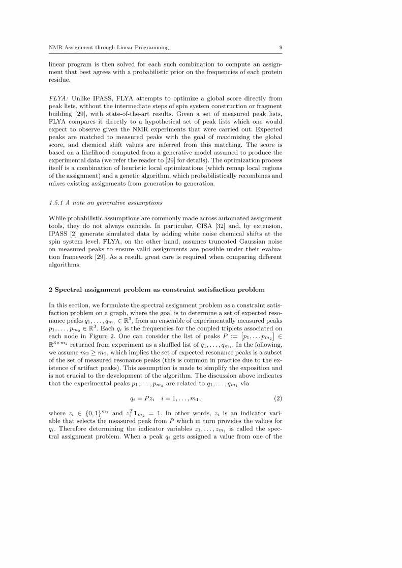
In this section, we formulate the spectral assignment problem as a constraint satis-faction problem on a graph, where the goal is to determine a set of expected reso-nance peaks q1, . . . , qm1 ∈ R3, from an ensemble of experimentally measured peaksp1, . . . , pm2 ∈ R3. Each qi is the frequencies for the coupled triplets associated oneach node in Figure 2. One can consider the list of peaks P :=

[p1, . . . pm2

]∈

R3×m2 returned from experiment as a shuffled list of q1, . . . , qm1 . In the following,we assume m2 ≥ m1, which implies the set of expected resonance peaks is a subsetof the set of measured resonance peaks (this is common in practice due to the ex-istence of artifact peaks). This assumption is made to simplify the exposition andis not crucial to the development of the algorithm. The discussion above indicatesthat the experimental peaks p1, . . . , pm2 are related to q1, . . . , qm1 via

qi = Pzi i = 1, . . . ,m1, (2)

where zi ∈ {0, 1}m2 and zTi 1m2 = 1. In other words, zi is an indicator vari-able that selects the measured peak from P which in turn provides the values forqi. Therefore determining the indicator variables z1, . . . , zm1 is called the spec-tral assignment problem. When a peak qi gets assigned a value from one of the

10 Jose F. S. Bravo-Ferreira et al.

zj

zi

Lij([1,1,0]Pzi, [1,1,0]Pzj)

Li(Pzi)

Fig. 5 Definition of cost for the assignment problem depicted in Figure 2. On each edge (i, j)in G = (V,E), there is a loss function Lij penalizing the difference in peaks’ frequencies, whileon each node a prior term Li is used to encourage the selection of certain peaks from P .

p1, . . . , pm2 , the three atoms that generate peak qi get assigned with resonancefrequencies.

In order to determine the indicator variables zi, i = 1, . . . ,m1, we solve aconstraint satisfaction type problem on the graph defined in Figure 2. Each edge(i, j) is associated with a penalty

Lij(BTijqi, B

Tijqj), (3)

where eachBij ∈{[

1 0 0]T,[0 1 0

]T,[0 0 1

]T,[1 1 0

]T,[0 1 1

]T,[1 0 1

]T}, and

Lij is some loss function. In words, we want to penalize the difference of certaincoordinates between qi and qj . Furthermore, each node i is associated with a reg-ularization Li : R3 → R that is used to impose some prior beliefs on qi. Thereforedetermining the indicator variables z1, . . . , zm1 can be done via solving

min{zi}

m1i=1

∑(i,j)∈E

Lij(BTijPzi, B

TijPzj) +

m1∑i=1

Li(Pzi) (4)

s.t. zi ∈ {0, 1}m2 , zTi 1m2 = 1 ∀i,m1∑i=1

zi ≤ 1m2 , (5)

an inference problem on a graphical model defined by G = (V,E). The last con-straint prevents selecting more than one measured peak from P for each qi. Weillustrate this construction in Figure 5.

We now turn to a reformulation of (4) that is closer in spirit to the most com-mon assignment procedure outlined in Section 1.2.1. Suppose there are n residuesin the protein. Based on the types of coupling detailed in Section 1.2, graph G infact takes the form in Figure 6, which is a path graph after an appropriate cluster-ing of the nodes into subgraphs G1, . . . , Gn, where we assume that each subgraphhas c nodes.

NMR Assignment through Linear Programming 11

Gk−1 Gk Gk+1

zizj

yk

Fig. 6 Redefining the variables z1, . . . , zm1 in (4) as y1, . . . , yn in (6) according to subgraphG1,. . . ,Gn. Grouping the nodes according to the dotted box induces a path graph.

Consider unit vectors yk, yk+1 ∈ {0, 1}mc2 , each representing the mc

2 ways ofassociating c measured peaks to each of the node clusters Gk, Gk+1, respectively(where the dimensionality follows from the fact that there are a total of m2 mea-sured peaks to assign to c nodes). Given some specific choice of yk, denoted by i,and some choice of yk+1, denoted by j, there is some total cost Wk,k+1(i, j) asso-ciated with the evaluation of the loss functions on our choice of peak assignments.Therefore, we have

min{yk}ni=1

n−1∑k=1

Tr(Wk,k+1yk+1yTk ) (6)

s.t. yk ∈ {0, 1}mc2 , yTk 1mc

2= 1, k = 1, . . . , n.

A(y1, . . . , yn) ≤ 1m2 (7)

That is, once we group the variables, as depicted in Figure 6, there are onlycost functions defined between the adjacent yk, yk+1, k = 1, . . . , n − 1. For eachpossible assignment of measured peaks to each set of adjacent subgraphs there isan associated cost, with the matrix Wk,k+1 representing the individual costs of allsuch assignment possibilities. The linear constraint A(y1, . . . , yn) ≤ 1m2 captures(5).

2.1 Outline of proposed method for solving (6)

Without constraint (7), the optimization problem (6) has cost defined on a pathgraph (since only yk and yk+1, k = 1, . . . , n−1 are coupled via some cost functions).This type of optimization problem can be solved using dynamic programming[6], and has a complexity of O(nm2c

2 ). More precisely, in order to get a dynamicprogramming problem, we turn to the construction of a new weighted graph G =(V, E) in Figure 7 with nmc

2 + 2 nodes. There are n + 2 layers, where each layerconsists of mc

2 nodes (except the first and last layer), and within each layer thereare no edges. Edges are formed between two adjacent layers of nodes with weights

12 Jose F. S. Bravo-Ferreira et al.

Wk−1,k Wk,k+1

Start End

nodesmc2

-th layerk -th layer(k + 1)-th layer(k − 1)Fig. 7 Illustration of finding a solution to (6) by solving a shortest path problem. Here, theshortest path is indicated in blue by dotted line that traverses from the “start” to the “end”node. Each set of nodes, e.g. nodes in the box, depicts all possible choices for each yi in (6).

defined by {Wk,k+1}n−1k=1 , where each Wk,k+1 ∈ Rm

c2×m

c2 . There are two extra

nodes in addition to the nmc2 nodes, denoted as the “start” and “end” nodes.

They are connected to the first and last groups of the nmc2 nodes as depicted in

Figure 7. The minimization problem in (6) without constraint (7) thus becomesa problem of tracing the shortest path from the start node to the end node, asdepicted in Figure 7. While this problem can be solved efficiently using dynamicprogramming, such an approach is not possible due to constraint (7). Therefore,in the next section, we turn to a linear programming formulation of the shortestpath problem, where (7) can be easily addressed.

3 Methodology

This section presents our general approach to NMR assignment, which we callLIAN (LInear Programming Assignment for NMR). We first describe how weconstruct an assignment graph G = (V, E) (different from G = (V,E) in (1) or(4)) on which we efficiently solve (6), a constrained shortest path problem whosesolution yields a valid assignment which approximately maximizes the expectedlog-likelihood under a given probabilistic model. We divide this section into twoparts: (1) defining the structure of the assignment graph (Section 3.1), and (2)solving the constrained shortest path problem (Section 3.2).

3.1 Building the assignment graph

The assignment graph G is a directed graph with n+2 layers, where n is the knownnumber of residues in the protein. This is illustrated in Figure 7, where a layer isa group of nodes, for example those in the red dotted box. The construction of thegraph proceeds in three steps:

1. Initial peak groupings: We first enumerate groups of measured peaks whosefrequencies are internally consistent. More precisely, we partition the variables

NMR Assignment through Linear Programming 13

z1, . . . , zm1 in (4) associated with nodes of G, by partitioning G into n sub-graphs G1, . . . , Gn (corresponding to n residues) as in Figure 6, and for eachpart we enumerate all the possible choices of assignments. For example, if eachGk has c number of zi’s associated with it, and each zi has m2 choices, thenthere are at most mc

2 choices for all the variables in Gk. This is too large in gen-eral, therefore we pick the possible values for all zi, zj associated with Gk suchthat Lij(B

TijPzi, B

TijPzj) is smaller than some threshold, for all i, j ∈ Gk. The

possible values of c zi’s within each part essentially corresponds to a choice ofc peaks from p1, . . . , pm2 . Therefore this is called the peak grouping procedure.We assume there are g choices for the variables in each Gk, which give g nodesin the k-th layer of the assignment graph.

2. Creating the graph nodes: A possible combination of peaks in P , that canbe assigned to the nodes in Gk, forms a node in a k-layer of G. Again, cor-responding to each layer (i.e. each residue), there are g nodes. To further cutdown the number of nodes, for each residue we enumerate the peak groupingsthat are sufficiently consistent with each residue, as determined by the differ-ence between the frequencies in the peak grouping and a prior, which is derivedfrom chemical shift statistics for each residue type stored in BMRB [30]. Thisstep associates a cost related to the log-likelihood of the assignment under theprior for each node. For the k-th residue, such a cost basically comes fromLi(Pzi), i ∈ Gk in (4). After this step, the k-th layer is left with gk nodes.

3. Creating the graph edges: Edges between two layers are added to the graphbetween any two nodes which have sufficiently consistent frequency assign-ments for the same atoms. Each edge contributes a cost commensurate with therelevant level of consistency. Such a cost comes from Lij(Bij

TPzi, BTijPzj), i ∈

Gk, j ∈ Gk+1 in (4).

We describe each of these steps in greater detail below.

3.1.1 Initial peak groupings

As explained in Section 2, our experimental data consists of a list of peaks, P :=[p1, . . . , pm], where each pi ∈ R3 corresponds to a set of atom frequencies. In orderto form nodes from this list of peaks, we group them in groups that are internallyconsistent, i.e., groups of peaks which assign approximately the same frequency tothe same atom.

As mentioned previously, a protein consists of n residues that have repeatedsets of atoms. The k-th residue rk contains atoms Nk, HNk , Cαk , Cβk . In subgraphGk,the nodes come from residues rk and rk+1 with triplets forming by Nk, HNk , Cαk ,Cβk , Cαk+1, Cβk+1. When considering an NMR dataset with three spectra, HSQC,HNCACB, and HN(CO)CACB, we expect Gk to contain seven nodes, comingfrom the fact that there are seven triplet interactions all involving the same Nkand HNk . Therefore, each Gk contributes to seven peaks in the three spectra.Some of these peaks will also share Cαk and Cβk frequencies. This is illustratedin Figure 3, where all seven peaks have consistent frequency values in N –HN

plane (and there are two peaks agreeing along the C dimension). This allows usto guess valid peak groupings associated with Gk. To this end, we make use ofan enumeration procedure (described in Appendix A) to enumerate all consistentpeak groupings, which are defined as groupings of seven peaks (or more, depending

14 Jose F. S. Bravo-Ferreira et al.

on the experiment set) where the frequencies associated with certain atoms do notdiffer by more than an experimentally-accepted threshold. We describe it moreconcisely here in the context of our example:

1. Select a reference spectrum (often called a fingerprint spectrum). This is typi-cally a spectrum from an experiment such as HSQC, which contains the peaksgenerated from the pairs (Nk,H

Nk ) as these spectra have higher sensitivity than

other experiments and are therefore less likely to be missing peaks. In principle,there should be n peaks in this spectra.

2. For each HSQC peak, enumerate all peaks in other spectra which are consistentwith peaks in the fingerprint spectrum along the N –HN dimensions, withinappropriate experimental thresholds (δ1, δ2).

3. Among all consistent peaks, identify all subsets which are consistent (withinexperimental threshold δ3) along the corresponding C dimension.

Spin systems: On some occasions, NMR practitioners perform this grouping proce-dure manually (or in a human-in-the-loop, computer-guided fashion). The group-ings of measured peaks are then summarized in the form of spin systems, byaveraging the frequencies assigned to each atom, thus producing a simple vectorof ”consensus” atom frequencies. As a result, data is sometimes summarized inthe spin system format rather as peak lists, and we can skip the grouping stepdescribed in this section. However, we note that this leads to some informationloss, as we lose information related to the level of agreement between frequenciesassigned to the same atom by different peaks.

3.1.2 Creating the graph nodes

Nodes in the assignment graph are subdivided into n + 2 layers, one for each ofthe n residues in the protein, and additional start and end layers to simplify theformulation of the problem. There are three broad classes of nodes:

1. Start and End nodes: The first layer and the n + 2-th layer consist of asingle node, used for convenience. These nodes help define the start and endposition of the shortest path we seek to find.

2. Dummy nodes: There is one such node for each of the n inner layers, andtheir function is to ensure the shortest path problem is feasible. There is apath from every node in layer k − 1 to the dummy node of layer k, and fromthis dummy node to every node in layer k + 1. If included in the final path,no frequencies will be assigned to the atoms in residue k, such that this nodeis equivalent to a null assignment for residue k, and incurs a high associatedcost.

3. Regular nodes: All other nodes in the graph represent a grouping of measuredpeaks, as defined in Section 3.1.1, which is consistent with the given residue.

In sum, there is exactly one start and one end node, and there are exactly ndummy nodes, one for each residue of the protein. However, given g valid peakgroupings (as defined in Section 3.1.1) we create gk ≤ g nodes in each layer. Thisis because any peak groupings which are not consistent with the prior on the atomfrequencies for a given residue are not instantiated, in order to reduce the overallsize of the graph. We formalize the process for eliminating nodes below, uponintroducing the edge cost definitions.

NMR Assignment through Linear Programming 15

xa1

N σ1

. . .

N σ...

xaoa

N σoa

µ

N

µa σa

Fig. 8 Generative model for an atom observed by oa peaks. A Gaussian prior for the frequencyof each atom, a, is assumed, with parameters µa and σa derived from chemical shift statisticsdeposited in BMRB [30]. The observed frequencies {xa1 , . . . , xaoa} of each atom are also assumedto be normally distributed, centered around the latent frequency of the atom and with (assumedknown) experimental variance σ1, . . . , σoa .

3.1.3 Creating the graph edges

After creating all n + 2 node layers, we connect nodes between each layer andthe subsequent layer. The edge creation step is most important because it is alsowhere we define the costs associated with each edge. In sum, we want this cost torepresent some notion of probabilistic agreement between our assumed generativemodel for the data and our set of observations.

Generative model: In Figure 2, atom a1 is shared by two nodes in graph G. Thatmeans two peaks observed in the spectra are associated with a1. We want to modelthe probability distribution of the observed peaks associated with an atom in com-mon. Many probabilistic cost functions would be reasonable, but for the purposesof this paper we assume that the prior on each atom’s frequency is Gaussian, andthat the experimental noise is also Gaussian (with mean 0). This is depicted inFigure 8 for an atom, a, for which we have oa distinct observations of its frequency,{xa1 , . . . , xaoa}. This implies that this atom is associated with oa peaks (or in otherwords associated with oa nodes in graph G in Figure 2). Such a generative modelprescribes a graphical model on graph G. Solving (4) amounts to performing infer-ence on zi’s under such a probabilistic model. This generative model is consistentwith much of the automated assignment literature (see, e.g. [32]) with the notableexception of FLYA, which assumes the experimental noise is a truncated Gaussian,in order to guarantee feasible assignments under its definition of a valid assignment[29].

Under this model, we define the score associated with each atom as

Definition 1 (Atom cost) The cost associated with atom a, with a normally dis-tributed prior N (µa, σa), and oa observations {xal }oal=1 defined by the peak grouping,also assumed to be normally distributed around the true frequency, µ, according toN (µ, σl) is defined as

cost (a, {xal }oal=1) , − logEµ∼N (µa,σa)

[oa∏l=1

f(xal | µ, σl)

]. (8)

16 Jose F. S. Bravo-Ferreira et al.

where f(· | u, v) is the Gaussian density with mean u and standard deviationv. This expectation works out to a simple expression involving the observations,experimental noise parameters, and the parameters of the prior distribution, asexplained in Appendix A.

Now, recall that if we select an edge between two nodes, node i in layer k,and node j in layer k + 1 in Figure 7, to be included in our path, we are indeedassigning observed peaks to the nodes in Gk and Gk+1. This implies that all theatoms involved in establishing the nodes (recall that each node is associated witha triplet or a pair of atoms) are assigned a frequency valued obtained from theobserved peaks. Then the generative model in Definition 1 determines how likelythese frequency assignments are under the assumed generative model, which will,in turn, help determine the likelihood of an edge (i, j) in Figure 7.

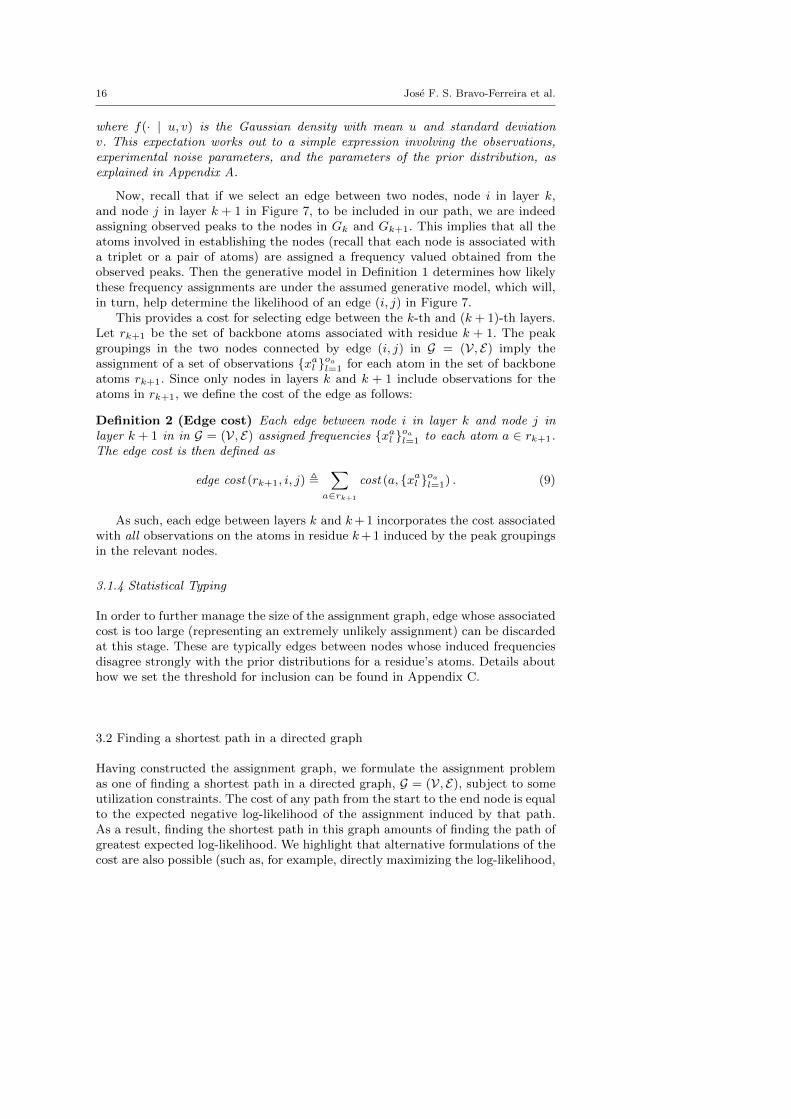
This provides a cost for selecting edge between the k-th and (k + 1)-th layers.Let rk+1 be the set of backbone atoms associated with residue k + 1. The peakgroupings in the two nodes connected by edge (i, j) in G = (V, E) imply theassignment of a set of observations {xal }oal=1 for each atom in the set of backboneatoms rk+1. Since only nodes in layers k and k + 1 include observations for theatoms in rk+1, we define the cost of the edge as follows:

Definition 2 (Edge cost) Each edge between node i in layer k and node j inlayer k + 1 in in G = (V, E) assigned frequencies {xal }oal=1 to each atom a ∈ rk+1.The edge cost is then defined as

edge cost (rk+1, i, j) ,∑

a∈rk+1

cost (a, {xal }oal=1) . (9)

As such, each edge between layers k and k+ 1 incorporates the cost associatedwith all observations on the atoms in residue k+ 1 induced by the peak groupingsin the relevant nodes.

3.1.4 Statistical Typing

In order to further manage the size of the assignment graph, edge whose associatedcost is too large (representing an extremely unlikely assignment) can be discardedat this stage. These are typically edges between nodes whose induced frequenciesdisagree strongly with the prior distributions for a residue’s atoms. Details abouthow we set the threshold for inclusion can be found in Appendix C.

3.2 Finding a shortest path in a directed graph

Having constructed the assignment graph, we formulate the assignment problemas one of finding a shortest path in a directed graph, G = (V, E), subject to someutilization constraints. The cost of any path from the start to the end node is equalto the expected negative log-likelihood of the assignment induced by that path.As a result, finding the shortest path in this graph amounts of finding the path ofgreatest expected log-likelihood. We highlight that alternative formulations of thecost are also possible (such as, for example, directly maximizing the log-likelihood,

NMR Assignment through Linear Programming 17

rather than the expected likelihood). However, the formulation presented here iscomputationally straightforward to implement, allowing us to quickly build largegraphs.

While an unconstrained shortest path problem is straightforward to solvethrough dynamic programming, our problem is not unconstrained, due to thefact that each observed datum (i.e. a measured peak) can only be utilized once ina valid assignment. This practical limitation can be concisely written as a linearconstraint, which fits into the constraint satisfaction framework we describe inSection 2.

In particular, recall that we had defined the assignment problem (6), whereyk ∈ {0, 1}m

c2 is a unit vector selecting a group of peaks for Gk. After reducing the

possible choices, we actually redefine our yk variables into yk ∈ {0, 1}gk , assuminggk valid combinations for layer k. We can further define

Xk,k+1 , ykyTk+1 ∈ {0, 1}gk×gk+1 , 1TgkXk,k+11gk+1 = 1 (10)

as a selection matrix, where Xk,k+1(i, j) = 1 implies that node i is selected in layerk and node j is selected in layer k + 1. Under this simple redefinition, Wk,k+1 ∈Rgk×gk+1 can also be easily understood as the matrix of edge costs between layersk and k + 1. That is

Wk,k+1(i, j) , edge cost(i, j) (11)

where edge cost(i, j) is the cost associated with the edge between node i in layerk and node j in layer k + 1. Also note that we need not worry about layers 0 andn + 1 to express the linear programming formulation of the problem, since thereis a single node in these two layers.

Finally, we can formulate the NMR assignment problem in terms of these newvariables:

Problem 1 (NMR assignment)

min{Xk,k+1}nk=0

n∑k=1

Tr(WTk,k+1Xk,k+1) (12)

s.t. Xk,k+1 ∈ {0, 1}gk×gk+1 , 1TgkXk,k+11gk+1 = 1, k = 1, . . . , n

XTk−1,k1gk−1 = Xk,k+11gk+1 , k = 1, . . . , nA(X1,21g2 , . . . , Xn,n+11gn+1) ≤ 1m2 (13)

Note the following details: A path constraint is included in the formulation,enforcing that the end node selected using Xk−1,k must coincide with the startnode selected using Xk,k+1. Compare to (6), the summation in the cost of (1)goes from k = 0 to k = n, which takes into account of the extra “start” and “end”node, and g0 = gn+1 = 1.

The problem as formulated above is equivalent to a constrained shortest pathproblem, and is NP-hard [1]. For small enough problems, integer linear program-ming (ILP) solvers such as Gurobi [23] can successfully solve the problem withshort runtimes. In our experience, this is often feasible whenever the input con-sists of a high quality set of nodes in each layer of G (e.g. when we have a setof reliable spin systems as input). However, for larger problems we can insteadmake use of linear programming relaxations of Problem 1. These relaxations canoccasionally return integer solutions (in which case the solution coincides with

18 Jose F. S. Bravo-Ferreira et al.

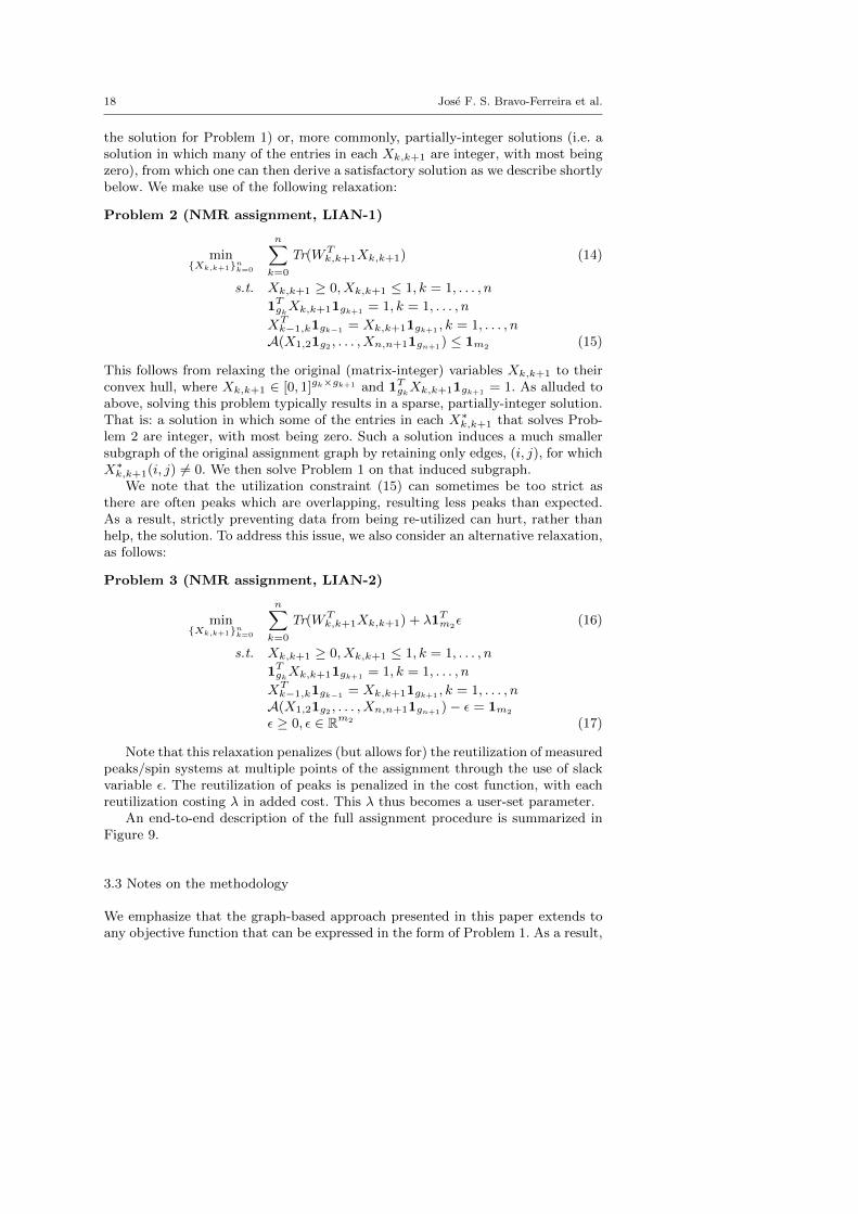
the solution for Problem 1) or, more commonly, partially-integer solutions (i.e. asolution in which many of the entries in each Xk,k+1 are integer, with most beingzero), from which one can then derive a satisfactory solution as we describe shortlybelow. We make use of the following relaxation:

Problem 2 (NMR assignment, LIAN-1)

min{Xk,k+1}nk=0

n∑k=0

Tr(WTk,k+1Xk,k+1) (14)

s.t. Xk,k+1 ≥ 0, Xk,k+1 ≤ 1, k = 1, . . . , n

1TgkXk,k+11gk+1 = 1, k = 1, . . . , n

XTk−1,k1gk−1 = Xk,k+11gk+1 , k = 1, . . . , nA(X1,21g2 , . . . , Xn,n+11gn+1) ≤ 1m2 (15)

This follows from relaxing the original (matrix-integer) variables Xk,k+1 to theirconvex hull, where Xk,k+1 ∈ [0, 1]gk×gk+1 and 1TgkXk,k+11gk+1 = 1. As alluded toabove, solving this problem typically results in a sparse, partially-integer solution.That is: a solution in which some of the entries in each X∗k,k+1 that solves Prob-lem 2 are integer, with most being zero. Such a solution induces a much smallersubgraph of the original assignment graph by retaining only edges, (i, j), for whichX∗k,k+1(i, j) 6= 0. We then solve Problem 1 on that induced subgraph.

We note that the utilization constraint (15) can sometimes be too strict asthere are often peaks which are overlapping, resulting less peaks than expected.As a result, strictly preventing data from being re-utilized can hurt, rather thanhelp, the solution. To address this issue, we also consider an alternative relaxation,as follows:

Problem 3 (NMR assignment, LIAN-2)

min{Xk,k+1}nk=0

n∑k=0

Tr(WTk,k+1Xk,k+1) + λ1Tm2

ε (16)

s.t. Xk,k+1 ≥ 0, Xk,k+1 ≤ 1, k = 1, . . . , n

1TgkXk,k+11gk+1 = 1, k = 1, . . . , n

XTk−1,k1gk−1 = Xk,k+11gk+1 , k = 1, . . . , nA(X1,21g2 , . . . , Xn,n+11gn+1)− ε = 1m2

ε ≥ 0, ε ∈ Rm2 (17)

Note that this relaxation penalizes (but allows for) the reutilization of measuredpeaks/spin systems at multiple points of the assignment through the use of slackvariable ε. The reutilization of peaks is penalized in the cost function, with eachreutilization costing λ in added cost. This λ thus becomes a user-set parameter.

An end-to-end description of the full assignment procedure is summarized inFigure 9.

3.3 Notes on the methodology

We emphasize that the graph-based approach presented in this paper extends toany objective function that can be expressed in the form of Problem 1. As a result,

NMR Assignment through Linear Programming 19

Fig. 9 Illustration of the full assignment procedure. (a) Possible chemical shift assignmentsare determined and enumerated for each residue, creating nodes in a graph. (b) Each node isstatistically typed against its residue’s distribution, and very low likelihood nodes are elimi-nated. (c) Edges are placed between nodes i, j in adjacent layers, k and k + 1 with weightequal to the posterior log-likelihood of the respective assignment. Empty nodes are added toeach residue and connected to every node in the preceding and succeeding layers with edgeweights equal to the threshold. (d) A longest path is found between the start and end nodes,subject to any additional constraints (e.g. that spin systems cannot be used more than once).

many different generative models can easily be accommodated by this methodol-ogy, and one is also not limited to maximizing an expected log-likelihood. As anexample, for each edge in the assignment graph connecting two nodes betweenlayers k and k + 1, which assign a set of observed chemical shifts to the atoms ofresidue k, one could solve a local maximum likelihood problem for that residue un-der the given observations. Doing so would enable a maximum likelihood estimateinstead.

20 Jose F. S. Bravo-Ferreira et al.

We also note that prior information or information from supporting experi-ments can also be accommodated, either by modifying the edge costs (through thematrices Wk,k+1) or by editing the assignment graph. As a concrete example, if onehad accurate information about the chemical shifts in a particular residue, rk+1,then one could specify tight priors, N (µa, σa), for each atom a in that residue,where µa would be set to the chemical shift implied by the prior information, andσa would be set to a value that accurately represents the uncertainty of that priorinformation. By doing so, Equations 8, 9, and 11 would result in entries of Wk,k+1

which are high for any chemical shift assignment that violates the prior informa-tion about residue rk+1, and low for any assignment consistent with that priorinformation, as desired. Additionally, one could also use this prior information todirectly edit the assignment graph (i.e. by removing any nodes which represent anassignment inconsistent with prior knowledge). This not only helps enforce priorknowledge, but also helps the efficiency of the algorithm.

In sum, while we describe a concrete end-to-end methodology using a specificgenerative model, the building blocks of our approach should prove more broadlyapplicable to a wider range of problems in spectral assignment.

4 Results

4.1 Simulated data

4.1.1 CISA

As a first sanity check, we tested our approach on the entirety of the benchmarkdataset developed by the authors of CISA in [32], as it provides a useful comparisonto many other fully automated algorithms on problems of small, medium, andlarge scale. This synthetic dataset is created by generating a simulated list ofspin systems from the ground-truth assignment values recorded in BMRB [30].White Gaussian noise is then added to the carbon atoms, with standard deviationsσα = 0.08 ppm, σβ = 0.16 ppm for the Cα and Cβ atoms, respectively, in the low-noise simulation, and σα = 0.16 ppm, σβ = 0.32 ppm in the high-noise simulation.For full details on the simulation scenario, we refer the reader to [32].

We compare the performance of LIAN to that of 4 different algorithms. Resultsfor MARS [25] and CISA [32] are both retrieved from the original CISA paper.We also compare with IPASS [2], although we note that the relevant paper doesnot mention adding noise to the spin systems (and, indeed, refers to a ”perfectconnectivity” scenario, which suggests that no noise is added). Finally, we alsoinclude a partial comparison with C-SDP [16], which is an earlier semidefiniteprogramming relaxation approach to the NMR assignment problem which we de-veloped, but which does not scale to larger proteins. The results for LIAN wereobtained by solving Problem 2, which typically produces a partially integer solu-tion. This partially integer solution induces a (much) smaller subgraph on whichwe can efficiently solve the original integer linear programming problem. Each rowis averaged over 100 simulations.

The results are summarized in Tables 1 and 2, for the two distinct noise levelsconsidered in [32]. We evaluate the results by calculating the precision and recallof the assignment algorithm. Let massigned be the number of assigned residues

NMR Assignment through Linear Programming 21

(i.e. non-dummy nodes in the path), mcorrect be the number of correctly assignedresidues, and massignable be the number of assignable residues (i.e. residues whichhave a ground-truth assignment). Then

precision , mcorrect/massigned

recall , mcorrect/massignable.

Table 1 Accuracy of assignment (precision/recall) of various algorithms and LP on syntheticspin systems with noise level (σα, σβ) = (0.08, 0.16). Results for MARS [25] and CISA takenfrom Table 2 in [32]. Results for IPASS taken from Table 3 in [2]. Results for C-SDP takenfrom Table 1 in [16].

Protein ID Length N1 MARS CISA IPASS C-SDP LIAN-1bmr4391 66 59 91/97 97/97 93/90 99/99 90/90bmr4752 68 66 98/97 96/94 100/94 100/100 100/100bmr4144 78 68 100/97 100/99 98/85 100/100 99/96bmr4579 86 83 97/91 98/98 100/98 100/100 100/99bmr4316 89 85 97/96 100/99 99/98 99/99 100/100bmr4288 105 94 97/95 98/98 100/98 99/99bmr4929 114 110 99/97 93/91 100/100 100/98bmr4302 115 107 95/92 96/95 100/99 100/99bmr4670 120 102 94/88 96/95 98/97 99/99bmr4353 126 98 91/85 96/95 99/93 95/95bmr4207 158 148 96/93 100/99 100/97 99/99bmr4318 215 191 88/81 87/84 100/98 98/98

1 Number of assignable spin systems in the BMRB data.

Table 2 Accuracy of assignment (precision/recall) of various algorithms and LP on syntheticspin systems with noise level (σα, σβ) = (0.16, 0.32). Results for MARS [25] and CISA takenfrom Table 2 in [32]. Results for IPASS taken from Table 3 in [2]. Results for C-SDP takenfrom Table 2 in [16].

Protein ID Length N1 MARS CISA IPASS C-SDP LIAN-1bmr4391 66 59 86/85 91/91 93/90 100/100 86/86bmr4752 68 66 91/90 90/88 100/94 99/99 100/100bmr4144 78 68 100/97 100/99 98/85 96/96 96/94bmr4579 86 83 79/75 80/80 100/98 100/100 100/99bmr4316 89 85 95/92 83/83 99/98 98/98 99/99bmr4288 105 94 95/93 91/91 100/98 99/99bmr4929 114 110 99/97 96/94 100/100 100/98bmr4302 115 107 82/80 91/91 100/99 99/99bmr4670 120 102 83/81 88/87 98/97 98/97bmr4353 126 98 83/80 90/90 99/93 95/95bmr4207 158 148 82/81 88/85 100/97 99/99bmr4318 215 191 84/75 74/70 100/98 98/98

1 Number of assignable spin systems in the BMRB data.

It can be seen that LIAN-1 achieves an assignment performance that generallyexceeds that of both CISA and IPASS, particularly on recall (with the aforemen-tioned caveat about the IPASS results, which may be overestimated by virtue

22 Jose F. S. Bravo-Ferreira et al.

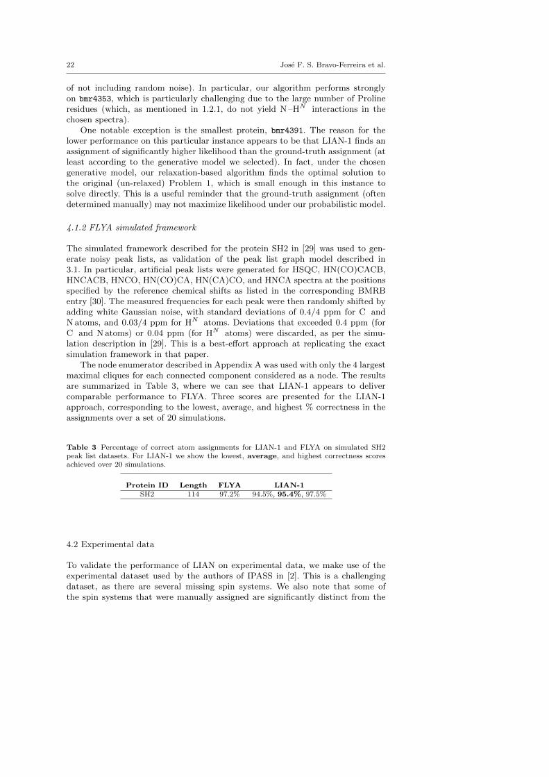
of not including random noise). In particular, our algorithm performs stronglyon bmr4353, which is particularly challenging due to the large number of Prolineresidues (which, as mentioned in 1.2.1, do not yield N –HN interactions in thechosen spectra).

One notable exception is the smallest protein, bmr4391. The reason for thelower performance on this particular instance appears to be that LIAN-1 finds anassignment of significantly higher likelihood than the ground-truth assignment (atleast according to the generative model we selected). In fact, under the chosengenerative model, our relaxation-based algorithm finds the optimal solution tothe original (un-relaxed) Problem 1, which is small enough in this instance tosolve directly. This is a useful reminder that the ground-truth assignment (oftendetermined manually) may not maximize likelihood under our probabilistic model.

4.1.2 FLYA simulated framework

The simulated framework described for the protein SH2 in [29] was used to gen-erate noisy peak lists, as validation of the peak list graph model described in3.1. In particular, artificial peak lists were generated for HSQC, HN(CO)CACB,HNCACB, HNCO, HN(CO)CA, HN(CA)CO, and HNCA spectra at the positionsspecified by the reference chemical shifts as listed in the corresponding BMRBentry [30]. The measured frequencies for each peak were then randomly shifted byadding white Gaussian noise, with standard deviations of 0.4/4 ppm for C andN atoms, and 0.03/4 ppm for HN atoms. Deviations that exceeded 0.4 ppm (forC and N atoms) or 0.04 ppm (for HN atoms) were discarded, as per the simu-lation description in [29]. This is a best-effort approach at replicating the exactsimulation framework in that paper.

The node enumerator described in Appendix A was used with only the 4 largestmaximal cliques for each connected component considered as a node. The resultsare summarized in Table 3, where we can see that LIAN-1 appears to delivercomparable performance to FLYA. Three scores are presented for the LIAN-1approach, corresponding to the lowest, average, and highest % correctness in theassignments over a set of 20 simulations.

Table 3 Percentage of correct atom assignments for LIAN-1 and FLYA on simulated SH2peak list datasets. For LIAN-1 we show the lowest, average, and highest correctness scoresachieved over 20 simulations.

Protein ID Length FLYA LIAN-1SH2 114 97.2% 94.5%, 95.4%, 97.5%

4.2 Experimental data

To validate the performance of LIAN on experimental data, we make use of theexperimental dataset used by the authors of IPASS in [2]. This is a challengingdataset, as there are several missing spin systems. We also note that some ofthe spin systems that were manually assigned are significantly distinct from the

NMR Assignment through Linear Programming 23

prior (this could be a legitimate biological phenomenon, as shielding effects re-sulting from the specific electronic environment of the protein shift the resonancefrequencies of atoms). LIAN-2 (Problem 3) was used throughout, with λ = 5. Re-sults are summarized in Table 4, which shows the number of correctly assignedresidues alongside the number of assigned residues for each methodology.

Table 4 Accuracy of assignment on four distinct spin system datasets provided by the authorsof IPASS. Results for other algorithms were obtained from [2].

Protein Length Manual1 Spins2 MARS IPASS C-SDP LIAN-2TM1112 89 83 81/85 55/63 71/72 50/85 74/81CASKIN 67 54 47/48 23/25 29/39 27/48 36/44VRAR 72 60 47/47 6/17 30/37 19/47 29/51HACS1 74 61 48/61 15/16 37/50 19/61 39/53

For each method, we show the results in the form #Correct/#Assigned, where #Correct isthe number of correctly assigned residues and #Assigned is the total number of assignedresidues.1 Number of manually assigned residues in the BMRB file.2 Correct/Total available spin systems, where spin systems are considered correct (i.e. notartifacts) if they were manually assigned by NMR practitioners. These numbers are takenfrom [2]. We note that there are meaningful differences between the spin system values andthe chemical shifts available publicly on BMRB, so the first number should be interpreted asan upper bound on the number of potentially assignable residues.

We see that LIAN-2 delivers state-of-the-art performance on this dataset interms of recall (albeit at the expense of lower precision relative to IPASS). How-ever, we note that the precision-recall threshold can be easily tuned by adjustingthe threshold score in the dummy nodes, and that once an assignment is pro-duced, validation of assigned spin systems can be made more easily by referringto the residue-level likelihood scores for debugging (which is why higher recall wasselected for in our thresholds).

An important observation provided by these experiments is that LIAN-2 isparticularly useful when datasets are of poor quality. In fact, we observe that thefinal solution in all these experiments reused several of the spin systems in multiplepositions, which would not have been possible under the standard formulationpresented in Problem 1. This illustrates the importance of correctly characterizingthe quality of the dataset through appropriate constraints on the problem.

5 Conclusion

This paper introduced a novel formulation of the spectral assignment problem inNMR as a constraint satisfaction problem. More specifically, we formulate it as aconstrained shortest path problem, for which near-optimal solutions can be foundvia linear programming relaxations. This approach has significant advantages overexisting approaches, as it treats spectral assignment as a global optimization prob-lem, without the need for intermediate steps (such as spin system creation) whichcan lead to information loss. Furthermore, the approach is amenable to multipleprobabilistic characterizations and could therefore accommodate complex charac-terizations of the generative model for the data (such as aminoacid-specific chem-ical shift correlations), which would simply result in different edge weights for the

24 Jose F. S. Bravo-Ferreira et al.

assignment graph introduced in Section 3. This approach could also straightfor-wardly accommodate other interactions often useful for assignment, such as theexistence of hydrogen-hydrogen interactions in NOE spectra, through additionallinear costs in the objective function.

Testing of our approach with a simplistic generative model on both simulatedand experimental data showed state-of-the-art performance. For synthetic, spinsystem data, our methodology’s performance matched or surpassed the best per-forming algorithms (IPASS, [2] and CISA, [32]), with a notable exception whereour algorithm found a higher likelihood assignment than the reference assignment,under our probabilistic model. For experimental, spin system data, our methodol-ogy improved upon state-of-the-art. For the higher dimensional problem of peaklist data, our preliminary studies indicate performance on par with state-of-the-artalgorithm, FLYA.

Our reformulation of the assignment problem permits a more realistic basis forassessment of complete automated structure determination, including ambiguousassignment and constraint methods [3].

Acknowledgements A.S. was partially supported by NSF BIGDATA award IIS-1837992,NIH/NIGMS award 1R01GM136780-01, award FA9550-17-1-0291 from AFOSR, the SimonsFoundation Math+X Investigator Award, and the Moore Foundation Data-Driven DiscoveryInvestigator Award. DC was supported by NIH GM-117212.

Conflict of interest

The authors declare that they have no conflict of interest.

Data and code availability

Data and preliminary (non-production) code used in simulations and tests is avail-able in the author’s repository at https://github.com/fsbravo/lipras.

References

1. Ahuja, R.K., Magnanti, T.L., Orlin, J.B.: Network Flows: Theory, Algorithms, and Ap-plications. Prentice-Hall, Inc., Upper Saddle River, NJ, USA (1993)

2. Alipanahi, B., Gao, X., Karakoc, E., Li, S.C., Balbach, F., Feng, G., Donaldson, L., Li, M.:Error tolerant NMR backbone resonance assignment and automated structure generation.J Bioinform Comput Biol 9(1), 15–41 (2011)

3. Allain, F., Mareuil, F., Menager, H., Nilges, M., Bardiaux, B.: ARIAweb: a server forautomated NMR structure calculation. Nucleic Acids Research 48(W1), W41–W47 (2020).DOI 10.1093/nar/gkaa362. URL https://doi.org/10.1093/nar/gkaa362

4. Bahrami, A., Assadi, A.H., Markley, J.L., Eghbalnia, H.R.: Probabilistic interaction net-work of evidence algorithm and its application to complete labeling of peak lists fromprotein nmr spectroscopy. PLOS Computational Biology 5(3), 1–15 (2009). DOI10.1371/journal.pcbi.1000307. URL https://doi.org/10.1371/journal.pcbi.1000307

5. Bailey-Kellogg, C., Chainraj, S., Pandurangan, G.: A random graph approach to NMRsequential assignment. J. Comput. Biol. 12(6), 569–583 (2005)

6. Bang-Jensen, J., Gutin, G.Z.: Digraphs: theory, algorithms and applications. SpringerScience & Business Media (2008)

NMR Assignment through Linear Programming 25

7. Baran, M.C., Huang, Y.J., Moseley, H.N.B., Montelione, G.T.: Automated analysis ofprotein nmr assignments and structures. Chemical Reviews 104(8), 3541–3556 (2004).DOI 10.1021/cr030408p. URL https://doi.org/10.1021/cr030408p. PMID: 15303826

8. Bartels, C., Guntert, P., Billeter, M., Wuthrich, K.: Garant-a general algorithm for res-onance assignment of multidimensional nuclear magnetic resonance spectra. Journal ofComputational Chemistry 18(1), 139–149. DOI 10.1002/(SICI)1096-987X(19970115)18:1〈139::AID-JCC13〉3.0.CO;2-H

9. Berman, H.M., Westbrook, J., Feng, Z., Gilliland, G., Bhat, T.N., Weissig, H., Shindyalov,I.N., Bourne, P.E.: The protein data bank. Nucleic Acids Res 28(1), 235–242 (2000). URLhttp://www.ncbi.nlm.nih.gov/pmc/articles/PMC102472/

10. Bodenhausen, G., J. Ruben, D.: Natural abundance nitrogen-15 nmr by enhanced het-eronuclear spectroscopy 69, 185–189 (1980)

11. Bromiley, P.: Products and convolutions of gaussian probability density functions. Tina-Vision Memo 3(4), 1 (2003)

12. Cavanagh, J., Fairbrother, W.J., Palmer, A.G., Rance, M., Skelton, N.J.: Protein NMRSpectroscopy, first edn. Academic Press Limited, 24-28 Oval Road, London NW1 7DX(1996)

13. Coggins, B.E., Zhou, P.: PACES: Protein sequential assignment by computer-assistedexhaustive search. Journal of Biomolecular NMR 26(2), 93–111 (2003)

14. Donald, B.R.: Algorithms in Structural Molecular Biology. The MIT Press (2011)15. Donald, B.R., Martin, J.: Automated nmr assignment and protein structure determina-

tion using sparse dipolar coupling constraints. Progress in Nuclear Magnetic ResonanceSpectroscopy 55(2), 101 – 127 (2009). DOI https://doi.org/10.1016/j.pnmrs.2008.12.001.URL http://www.sciencedirect.com/science/article/pii/S0079656509000119

16. Ferreira, J.F.S.B., Khoo, Y., Singer, A.: Semidefinite programming approach for thequadratic assignment problem with a sparse graph. Comp. Opt. and Appl. 69(3),677–712 (2018). DOI 10.1007/s10589-017-9968-8. URL https://doi.org/10.1007/s10589-017-9968-8

17. Grzesiek, S., Bax, A.: Correlating backbone amide and side chain resonances in largerproteins by multiple relayed triple resonance nmr. Journal of the American ChemicalSociety 114(16), 6291–6293 (1992). DOI 10.1021/ja00042a003. URL https://doi.org/10.1021/ja00042a003

18. Grzesiek, S., Bax, A.: An efficient experiment for sequential backbone assignment ofmedium-sized isotopically enriched proteins. Journal of Magnetic Resonance (1969)99(1), 201 – 207 (1992). DOI https://doi.org/10.1016/0022-2364(92)90169-8. URLhttp://www.sciencedirect.com/science/article/pii/0022236492901698

19. Grzesiek, S., Bax, A.: Amino acid type determination in the sequential assignment proce-dure of uniformly 13C/15N-enriched proteins. J Biomol NMR 3(2), 185–204 (1993)

20. Guerry, P., Herrmann, T.: Comprehensive Automation for NMR Structure Determi-nation of Proteins, pp. 429–451. Humana Press, Totowa, NJ (2012). DOI 10.1007/978-1-61779-480-3 22. URL https://doi.org/10.1007/978-1-61779-480-3_22

21. Guntert, P., Buchner, L.: Combined automated noe assignment and structure calcu-lation with cyana. Journal of Biomolecular NMR 62(4), 453–471 (2015). DOI10.1007/s10858-015-9924-9. URL https://doi.org/10.1007/s10858-015-9924-9

22. Guntert, P., Salzmann, M., Braun, D., Wuthrich, K.: Sequence-specific nmr assignment ofproteins by global fragment mapping with the program mapper. Journal of BiomolecularNMR 18(2), 129–137 (2000). DOI 10.1023/A:1008318805889. URL https://doi.org/10.1023/A:1008318805889

23. Gurobi Optimization, L.: Gurobi optimizer reference manual (2020). URL http://www.gurobi.com

24. Hitchens, T.K., Lukin, J.A., Zhan, Y., McCallum, S.A., Rule, G.S.: MONTE: An auto-mated Monte Carlo based approach to nuclear magnetic resonance assignment of proteins.Journal of Biomolecular NMR 25(1), 1–9 (2003)

25. Jung, Y.S., Zweckstetter, M.: Mars - robust automatic backbone assignment of proteins.Journal of Biomolecular NMR 30(1), 11–23 (2004). DOI 10.1023/B:JNMR.0000042954.99056.ad. URL http://dx.doi.org/10.1023/B%3AJNMR.0000042954.99056.ad

26. Karjalainen, M., Tossavainen, H., Hellman, M., Permi, P.: HACANCOi: a new HI±-detected experiment for backbone resonance assignment of intrinsically disordered pro-teins. J Biomol NMR (2020)

27. Leutner, M., Gschwind, R.M., Liermann, J., Schwarz, C., Gemmecker, G., Kessler, H.: Au-tomated backbone assignment of labeled proteins using the threshold accepting algorithm.Journal of Biomolecular NMR 11(1), 31–43 (1998)

26 Jose F. S. Bravo-Ferreira et al.

28. Lian, L.Y., Barsukov, I.L.: Resonance Assignments, chap. 3, pp. 55–82. Wiley-Blackwell(2011). DOI 10.1002/9781119972006.ch3. URL https://onlinelibrary.wiley.com/doi/abs/10.1002/9781119972006.ch3

29. Schmidt, E., Guntert, P.: A new algorithm for reliable and general NMR resonance as-signment. Journal of the American Chemical Society 134(30), 12817–12829 (2012). DOI10.1021/ja305091n. URL https://doi.org/10.1021/ja305091n. PMID: 22794163

30. Ulrich, E.L., Akutsu, H., Doreleijers, J.F., Harano, Y., Ioannidis, Y.E., Lin, J., Livny, M.,Mading, S., Maziuk, D., Miller, Z., Nakatani, E., Schulte, C.F., Tolmie, D.E., Kent Wenger,R., Yao, H., Markley, J.L.: Biomagresbank. Nucleic Acids Research 36(suppl 1), D402–D408 (2008). DOI 10.1093/nar/gkm957. URL http://nar.oxfordjournals.org/content/36/suppl_1/D402.abstract

31. Volk, J., Herrmann, T., Wuthrich, K.: Automated sequence-specific protein NMR assign-ment using the memetic algorithm MATCH. Journal of Biomolecular NMR 41(3), 127–138(2008)

32. Wan, X., Lin, G.: CISA: Combined NMR resonance connectivity information determina-tion and sequential assignment. IEEE/ACM Transactions on Computational Biology andBioinformatics 4(3), 336–348 (2007). DOI 10.1109/tcbb.2007.1047

33. Yang, Y., Fritzsching, K.J., Hong, M.: Resonance assignment of the NMR spectra of disor-dered proteins using a multi-objective non-dominated sorting genetic algorithm. Journalof Biomolecular NMR 57(3), 281–296 (2013)

34. Zeng, J., Zhou, P., Donald, B.R.: HASH: a program to accurately predict protein Hα shiftsfrom neighboring backbone shifts. J. Biomol. NMR 55(1), 105–118 (2013)

35. Zimmerman, D.E., Kulikowski, C.A., Huang, Y., Feng, W., Tashiro, M., Shimotaka-hara, S., ya Chien, C., Powers, R., Montelione, G.T.: Automated analysis of proteinnmr assignments using methods from artificial intelligence. Journal of Molecular Bi-ology 269(4), 592 – 610 (1997). DOI https://doi.org/10.1006/jmbi.1997.1052. URLhttp://www.sciencedirect.com/science/article/pii/S0022283697910524

NMR Assignment through Linear Programming 27

A - Grouping Peaks

As we mentioned in Section 3.1.1, grouping consistent peaks together is a crucial step in thegraph creation process for G = (V, E). One would wish the enumeration of valid assignments tobe as thorough as possible. We can effectively enumerate peak groupings to construct nodes inG by matching measured and expected peaks in a self-consistent way. In particular, we expecta specific set of peaks due to N –HN from residue k (see Figure 10 for a standard examplewith three experiments) where the values of these peaks in R3 along certain dimensions areconsistent. If there are n residues, we should have n sets of such expected peaks. Therefore,each layer in G = (V, E) in principle should have n nodes, although in practice there are morenodes due ambiguities.

Expected peaks

S1 S2 S3

Nk Cα

Ckβ

HkN

Ckα Ck

O

Ok

Nk-1 Cα

Ck-1β

Hk-1N

Ck-1α Ck-1

O

Ok-1

residue k-1 residue k

Nk

HkN

Nk

HkN

Nk

HkN

Nk

HkN

Nk

HkN

Nk

HkN

Nk

HkN

Ckα Ck

αCkβ Ck

β Ck-1α Ck-1

β

Fig. 10 With three NMR experiments (often HSQC, HNCACB, and HN(CO)CACB) wegenerally expect 7 distinct peaks for each base N –HN pair in a residue, k. These peaks mustbe consistent - that is, the frequencies assigned to the same atom by two different peaks mustbe approximately the same up to some experimental tolerance. In principle, there should be nsets of such 7 peaks, one for each residue.

The notion of consistency can help significantly simplify the enumeration process (whichwould otherwise result in an exponential number of nodes). In order to efficiently enumerateconsistent peak groupings, we do the following. Let S1, . . . ,SL be collections of measured peaklists corresponding to different heteronuclear experiments, i.e. ∪Ll=1Sl := [p1, . . . , pm2 ]. In thecase of Figure 10, L = 3, as we have peaks from three experiments. Now from these m2

experimental peaks we form all combinations of seven peaks that each consists of one peakfrom S1, two peaks from S2, and four peaks from S3 using the following criteria.

– For any pair of pu, pv in a combination of seven peaks,

|pu(1)− pv(1)| ≤ δ1|pu(2)− pv(2)| ≤ δ2.

This means that the frequencies of the seven peaks in the N –HN dimension have tocoincide up to tolerance δ1, δ2.

– Furthermore, for a combination of seven peaks, let pu, pv be the two peaks in S2. Thesepeaks should coincide with two of the peaks in S3 (denoted pi, pj) up to tolerance δ3, i.e.

|pu(3)− pi(3)| ≤ δ3|pv(3)− pj(3)| ≤ δ3

along the C dimension.

B - Atom cost

Recall that we defined the cost of an atom, a, under a given set of assigned observations,{xl}oal=1 as

28 Jose F. S. Bravo-Ferreira et al.

Definition 3 (Atom cost) The cost associated with atom a, with a normally distributedprior N (µa, σa), and oa observations {xal }

oal=1 defined by the peak grouping, also assumed to

be normally distributed around the true frequency, µ, according to N (µ, σl) is defined as

cost(a, {xal }

oal=1

), − logEµ∼N (µa,σa)

[oa∏l=1

f(xal | µ, σl)]. (18)

where f(· | u, v) is the Gaussian density with mean u and standard deviation v.

This is Definition 1 in the main text. Note that the term inside the expectation is aproduct of oa univariate Gaussian probability density functions. Furthermore, expanding theexpectation, we note that

Eµ

[oa∏l=1

f(xal | µ, σl)]

=

∫ +∞

−∞f(µ | µa, σa)

oa∏l

f(xal | µ, σl)dµ (19)

=

∫ +∞

−∞f(µ | µa, σa)

oa∏l

f(µ | xal , σl)dµ (20)

by symmetry. Using a standard result regarding the product of univariate Gaussian PDFs (see,e.g., [11]), we can write

Eµ

[oa∏l=1

f(xal | µ, σl)]

=

∫ +∞

−∞f(µ | µa, σa)

oa∏l

f(µ | xal , σl)dµ (21)

=

∫ +∞

−∞Zaf(µ |Ma, Σa)dµ (22)

= Za (23)

where

Σa =

(1

σ2a

+

oa∑l=1

1

σ2l

)−1/2

(24)

Ma =

(µa

σ2a

+

oa∑l=1

xl

σ2l

)Σ2a (25)

Za =1

(2π)oa/2

√Σ2a

σ2a

∏oal=1 σ

2l

exp

[−

1

2

(µ2aσ2a

+

oa∑l=1

x2lσ2l

−M2a

Σ2a

)]. (26)

We see that this choice of cost function is therefore computationally advantageous, as thedesired expectation is a simple function of the observations, {xl}oal=1 and of the distributionalparameters of the prior, (µa, σa) and experiments, {σl}oal=1. That said, it is certainly not theonly cost function that one could use. As an example, we could instead solve a maximumlikelihood problem for each peak grouping that would assign the highest likelihood frequencyto each atom, given the prior and the observations. The exploration of alternative cost functionsis left for future work.

C - Statistical Typing

Statistical typing is a process that happens both during the node and edge creation steps.In particular, we want to avoid the creation of nodes and edges which are too unlikely toconstitute a valid assignment. The way we action on this notion is to define a threshold belowwhich we would rather have a null assignment than the assignment induced by the relevantnodes. This threshold also determines the cost of the edges to (and from) the dummy nodes,which are therefore the highest cost edges in the graph.

For all simulations in this paper, we use the following definition:

NMR Assignment through Linear Programming 29

Definition 4 (Atom cost threshold) The maximum allowable cost associated with atoma, with an expected frequency, µ, distributed according to the normally distributed priorN (µa, σa), and a total of oa expected observations is given by:

threshold (a) , cost(a, {wal }oal=1) (27)

wherewal = µa + δσa + (−1)l+1δσl. (28)

That is, we define the maximum allowable cost for atom a by setting {xal }oal=1 in Definition

1 to {wal }oal=1, which constitute an adversarial realization of the observations. In this realization,

the mean of the observations is ≈ δ standard deviations away from the prior mean, and theobservations are split into two clusters, 2δ experimental standard deviations apart.