
NMF HANDBOOK · NMF HANDBOOK An Introduction to the Neutral Model Format NMF version 3.02 Nov 1996...
66
NMF HANDBOOK An Introduction to the Neutral Model Format NMF version 3.02 Nov 1996 Per Sahlin Building Sciences KTH 100 44 STOCKHOLM [email protected] ASHRAE RP-839
Transcript of NMF HANDBOOK · NMF HANDBOOK An Introduction to the Neutral Model Format NMF version 3.02 Nov 1996...
NMF HANDBOOKAn Introduction to the Neutral Model Format
NMF version 3.02
Nov 1996
Per Sahlin Building Sciences KTH 100 44 STOCKHOLM [email protected] ASHRAE RP-839
2
Contents
1. ABOUT THIS TEXT ................................................................................................................... 4
2. INTRODUCTION ........................................................................................................................ 5
2.1 MODULAR SIMULATION ENVIRONMENTS........................................................................................ 52.1.1 Separation of Modelling and Solving Activities..................................................................... 62.1.2 Target Users and Software Structure..................................................................................... 62.1.3 Available and Emerging MSEs.............................................................................................. 6
2.2 THE NEUTRAL MODEL FORMAT ..................................................................................................... 82.3 CURRENT DEVELOPMENT............................................................................................................... 8
3. BASIC CONSTRUCTS.............................................................................................................. 10
3.1 A SIMPLE EXAMPLE - THERMAL CONDUCTANCE........................................................................... 103.2 WHAT IS A CONTINUOUS MODEL? ................................................................................................. 113.3 NOMENCLATURE: COMMENTS, RESERVED WORDS, ETC................................................................ 113.4 ABSTRACT SECTION .................................................................................................................... 113.5 EQUATION DECLARATIONS.......................................................................................................... 113.6 MODEL BOUNDARIES - LINKS ..................................................................................................... 123.7 VARIABLE AND PARAMETER DECLARATIONS ................................................................................ 14
3.7.1 Type.................................................................................................................................... 143.7.2 Name .................................................................................................................................. 143.7.3 Role .................................................................................................................................... 143.7.4 Description ......................................................................................................................... 143.7.5 IN/OUT Discussion............................................................................................................. 143.7.6 Order of Declared Quantities.............................................................................................. 15
3.8 PARAMETER PROCESSING............................................................................................................. 153.8.1 Restriction on Repeated Assignments.................................................................................. 15
3.9 GLOBAL DECLARATIONS.............................................................................................................. 173.9.1 Name .................................................................................................................................. 183.9.2 Unit .................................................................................................................................... 183.9.3 Kind.................................................................................................................................... 183.9.4 The GENERIC Reserved Word............................................................................................ 19
3.10 FILE STRUCTURE....................................................................................................................... 20
4. MODELLING GUIDELINES ................................................................................................... 21
4.1 THINKING EQUATION DECLARATION - NOT ASSIGNMENT PROGRAMMING...................................... 214.1.1 Algorithmic Models ............................................................................................................ 214.1.2 Equation Models................................................................................................................. 214.1.3 Discussion .......................................................................................................................... 22
4.2 FINDING COMPONENT MODEL BOUNDARIES................................................................................. 224.3 THE RIGHT NUMBER OF EQUATIONS IN EACH MODEL ................................................................... 234.4 A USEFUL SPECIAL CASE - BI-DIRECTIONAL FLOW........................................................................ 24
4.4.1 The Multizone Air-Exchange Models.................................................................................. 244.4.2 NMF Examples .................................................................................................................. 25
4.5 REAL-LIFE EQUATIONS................................................................................................................ 294.5.1 User-Independent Initial Guesses........................................................................................ 304.5.2 Additional Features of the Multizone Air Exchange Model Family..................................... 31
4.6 DECLARATION OF BAD INVERSES.................................................................................................. 324.7 TARGET ENVIRONMENT CAPABILITIES........................................................................................... 32
5. ADVANCED CONSTRUCTS.................................................................................................... 33
5.1 VECTORS AND MATRICES............................................................................................................. 335.1.1 Model Parameter Declaration and Processing.................................................................... 355.1.2 A PDE Example: 1D Heat Equation ................................................................................... 35
5.2 USER DEFINED FUNCTIONS.......................................................................................................... 38
3
5.2.1 Commented BNF Example: NMF Function Definitions....................................................... 385.2.2 Functions in NMF Notation ................................................................................................415.2.3 Functions in F77 or C......................................................................................................... 415.2.4 Target Environment Functions - EXTERNAL...................................................................... 425.2.5 Discussion .......................................................................................................................... 43
5.3 NMF VARIABLE ASSIGNMENTS.................................................................................................... 435.3.1 Locally Assigned Variables................................................................................................. 44
5.3.1.1 Discussion ..................................................................................................................................485.3.2 Assigned State Variables..................................................................................................... 49
5.3.2.1 Discussion ..................................................................................................................................515.4 MULTIPLE MODES AND DISCRETE EVENTS.................................................................................... 52
5.4.1 A General Framework for Multimode Models ..................................................................... 545.4.2 Signaling Discrete Events ................................................................................................... 54
5.4.2.1 Discussion ..................................................................................................................................55
6. SOLVED NMF PROBLEMS..................................................................................................... 56
6.1 EXERCISE 1 - A BASIC MECHANICS PROBLEM................................................................................ 566.2 SOLUTION TO EXERCISE 1 ............................................................................................................ 56
6.2.1 NMF Models....................................................................................................................... 566.2.2 Input file for IDA Solver..................................................................................................... 61
APPENDIX A A SYSTEM MODEL EXAMPLE IN FUTURE NMF (V. 4) ............................. 66
NMF Model Examples
NMF MODEL 3-1: TQ_CONDUCTANCE...................................................................................... 10NMF MODEL 4-1: SIMPLE_BDZONE........................................................................................... 26NMF MODEL 4-2: SIMPLE_BDLEAK........................................................................................... 27NMF MODEL 4-3: SIMPLE_VXSUPT............................................................................................ 29NMF MODEL 5-1: LESS_SIMPLE_BDZONE ................................................................................ 34NMF MODEL 5-2: TQ_HOM_WALL............................................................................................. 38NMF MODEL 5-3: FUNCTION HOM_WALL................................................................................ 42NMF MODEL 5-4: FUNCTION HOM_WALL2 .............................................................................. 42NMF MODEL 5-5: TQ_HOM_WALL_WRAPPED ......................................................................... 46NMF MODEL 5-6: TQ_HOM_WALL_WRAPPED2 ....................................................................... 51NMF MODEL 5-7: THERMOSTAT_NO_EVENTS ........................................................................ 53NMF MODEL 6-1: POINT_MASS .................................................................................................. 58NMF MODEL 6-2: SPRING ............................................................................................................ 59NMF MODEL 6-3: DAMPER..........................................................................................................59
Figures
FIGURE 3-1. A THERMAL CONDUCTANCE WITH A LINEAR RELATIONSHIP BETWEENHEATFLUX, Q, AND TEMPERATURE DIFFERENCE, T1 - T2.......................................... 10
FIGURE 3-2. TWO CONNECTED TQ_CONDUCTION INSTANCES........................................... 13FIGURE 4-1..................................................................................................................................... 23FIGURE 4-2..................................................................................................................................... 23FIGURE 5-1. A HOMOGENEOUS WALL DIVIDED INTO SEVERAL LAYERS.......................... 35FIGURE 5-2. THERMOSTAT CHARACTERISTIC........................................................................ 49FIGURE 5-3. A MODEL WITH FOUR MODES, ARROWS REPRESENT POSSIBLE MODE
SWITCHES. EACH SWITCH WILL HAVE AN ASSOCIATED CONDITION...................... 52FIGURE 6-1. SIMPLE MECHANICAL SYSTEM........................................................................... 56
4
1. About This TextThe NMF Handbook provides guidelines for modelling with the Neutral ModelFormat. It is intended to be a first text on the subject, but some topics should also beuseful for an NMF modeller with previous experience. The reader is assumed to havemathematical modelling experience and also to be familiar with the general softwareand hardware tools that are necessary for NMF modelling, such as a compiler and atarget simulation environment. NMF is normally used in conjunction with a specificsimulation environment, such as TRNSYS. However, this text is environmentindependent, except for some exercises, where an IDA Solver file is used as a concreteexample. The text is a complement to the NMF report The Neutral Model Format forBuilding Simulation and many grammatical details of NMF and other specific rules arenot repeated here. The following material is useful to have at hand during reading:
1. The ASHRAE NMF Translator program and associated sample NMF files. Thismaterial is available at ftp://urd.ce.kth.se/pub/rp839/.
2. The NMF Report The Neutral Model Format for Building Simulation, available atftp://urd.ce.kth.se/pub/reports/nmfre302.ps.
3. An NMF compatible simulation environment and an associated NMF translator formodel testing, available, for example, at http://www.brisdata.se/.
This document is also available in electronic form in Rich Text Formatftp://urd.ce.kth.se/pub/reports/handbook.rtf and in Postscriptftp://urd.ce.kth.se/pub/reports/handbook.ps.
5
2. IntroductionThe author of this handbook has for some time worked with new simulation techniquesand languages for continuous modular systems. These techniques are applicable to alarge class of static and dynamical simulation problems in, e.g., the building, energyand process industries. One important aspect of this work has been involvement in thedefinition of the Neutral Model Format (NMF), for expression of component levelsimulation models.
In the present version of NMF, component models (primitive models) are automaticallytranslated from NMF to the proprietary format of the target simulation environment.For example, an NMF model of an axial fan is used to generate an axial fan class in,e.g. IDA, or a corresponding type subroutine in TRNSYS or HVACSIM+. The class isthen instantiated in the target environment. The instances are furnished with suitableparameters, and incorporated into a system model. System modelling is notencompassed by the present version of NMF, i.e. TRNSYS decks cannot be generatedautomatically at this stage, only types.
In the next two sections we will give a brief overview of current work on modularsimulation methods, mainly in the context of building simulation, and of thebackground of the Neutral Model Format. These sections may be omitted without lossof continuity.
2.1 Modular Simulation EnvironmentsPhysical systems that are simulated in Modular Simulation Environments (MSEs) aremodular in nature, i.e. they naturally decompose into subsystems. Frequently, identicalsubsystems are repeated a number of times in a model, a fact that is taken advantage ofin many tools. Furthermore, the systems should have a basically continuous behavior,meaning that equations used to describe them, as well as forcing functions, will have alimited number of discontinuities. Purely event driven systems are excluded.
If characterized by equations, the physical systems under consideration will requireboth algebraic and differential equations. Differential equations can be either ordinary(ODE) or partial (PDE), although current tools, and the present NMF, require thatPDEs are explicitly discretized in space and thus turned into ODEs. Note that incontrast to many widely used commercial tools, the simulation environments we areconcerned with here are not limited to ODEs only. They allow a free mixture ofalgebraic and ordinary differential equations generally referred to as differential-algebraic systems of equations (DAE).
Furthermore, the simulation tools under discussion are rarely used for applicationswhere a strict formalism for generating governing equations exists. In, e.g., electricalcircuit analysis, multibody mechanics, or structural analysis special purpose systemsmay be more advantageous.
Examples of physical systems that fit this description can be found in many fields.Chemical process plant simulation is a significant area of application. Energydistribution networks and plants is another. The author of this handbook has mainly
6
worked with building related systems and important applications within this field are:thermal processes in walls and spaces; air and water based distribution systems andplants; and automatic control.
2.1.1 Separation of Modelling and Solving ActivitiesIn contrast to mainstream design tools in, e.g., building simulation, MSEs separatestrictly between the modelling and subsequent system solution activities. A modellingtool is often used for model formulation. This tool generates a system model, generallyexpressed in a modelling language. The model is then treated by a solver. Animportant benefit of a separate solver is that it may be altered or even exchanged withminimal interference with the modelling environment. Some MSEs rely on regularprogramming languages as part of their system model description. For these,component models are typically described as subroutines with prescribed structure,while interconnection of pre-programmed component models into system models isdescribed with a dedicated language. Other environments have complete modellinglanguages, which describe component as well as system behavior.
Key characteristics of the modelling language, such as expressiveness and level ofstandardization, are critical to the usefulness and development potential of the overallMSE. The Neutral Model Format is part of such a modelling language. NMF can betranslated into subsets of several complete target modelling languages; it does notcover all constructs in any of the present targets, just a sufficient “commondenominator.”
2.1.2 Target Users and Software StructureMost of the simulation tools under discussion are intended for quite sophisticatedusers, who are well versed in mathematical modelling, numerical methods andadvanced use of computers. These tools are not directly suited for designers, withoutspecial simulation expertise, that use simulation as one of several methods for designevaluation. However, for the expert, they generally provide an efficient environmentfor model building, simulation and analysis.
Other tools, e.g. EKS and IDA, are primarily intended for efficient design toolproduction, and the normal end user will rarely interact directly with the underlyingMSE techniques.
2.1.3 Available and Emerging MSEsA few tools and environments with the discussed main characteristics are alreadymatured and available and others are under development:
TRNSYS was developed during the seventies at the Solar Energy Lab at theUniversity of Wisconsin. It was one of the first modular simulation solvers for DAEsand it is distributed as a Public Domain product. It has recently been furnished with asimultaneous solver, i.e. a solver which solves all equations simultaneously. Severalcompatible commercial modelling tools have been developed, e.g. PRESIM
(http://www.engr.wisc.edu/centers/sel/trnsys/index.html).
HVACSIM+ is a solver with similar characteristics as TRNSYS in terms of modelformat and structure, but more recent numerical techniques than in the original TRNSYS
7
are utilized. It was developed by NIST in Maryland and released in the mid eighties ona Public Domain basis [Clark 1985]
SANDYS is a general DAE solver and textual modelling environment developed byASEA, Sweden, in the early eighties. It is commercially available from ABB CorporateResearch [Ohlsson 1991].
ALLAN.Simulation is a graphical modeller and solver combination developed by Gazde France and CISI Engineering. It is since a few years commercially available from thedevelopers [Jeandel 1993].
ESACAP is a DAE solver by Elektronikcentralen in Denmark. It is commerciallyavailable from STANSIM, Denmark.
DYMOLA is a commercial modelling tool with symbolic algebra capabilities andinterfaces to several solvers. Available from DYNASIM, Lund, Sweden(http://www.dynasim.se/).
CLIM 2000, a graphical modelling tool for building applications, is developed byElectricite de France for internal use [Bonneau 1993].
IDA , a graphical modelling environment (IDA Modeller) and solver (IDA Solver). Thelatter is available from Bris Data AB, Stockholm, Sweden. IDA Modeller will bereleased during 1996 [Bring 1995].
MS1 is a graphical multi input language modeller with interfaces to several solvers byLorenz Simulation, Liege, Belgium in cooperation with Electricite de France [Lorenz1990].
ISE, a graphical programmable front end that can be used with several buildingsimulation engines such as TRNSYS and COMIS. A TRNSYS application (IIisibat) isavailable from the developers at CSTB, France [Pelletret 1995].
SPARK is a solver and graphical model editor under development at LBL, Berkeley,California [Buhl 1993].
OMSIM is a graphical modelling tool under development at the Dept. of AutomaticControl at the Lund Institute of Technology, Sweden (http://control.lth.se/~cace/).
EKS is a C++ toolkit for development of energy related simulation design tools, byamong others the Univ. of Strathclyde, Scotland [Clarke 1993].
SMILE, a general purpose differential-algebraic modelling and simulation environmentdeveloped primarily for energy related problems. Modelling language, model library,and related software is under development at the Technical University of Berlin(http://www.cs.tu-berlin.de/~smile/synopsis.html).
8
THUVAC is a graphical modelling tool and solver for simulation of HVAC relatedmodular systems. It is under development at Dept. of Thermal Energy, Tsinghua Univ.,Beijing, China [Yi Jiang 1994]
2.2 The Neutral Model FormatWithout a comprehensive, validated library of ready made component models in arelevant application area most simulation environments are rather useless. To developall necessary models from scratch is, in many projects, quite unrealistic. And since thecost of developing a substantial library easily exceeds the development cost of thesimulation tool itself, it is important to be able to reuse what other people already havedone. This was the basic motivation for proposing a text based neutral model format tothe building simulation community in 1989 [Sahlin and Sowell 1989]. Since then theproposal has attracted a great deal of interest from environment developers and usersin several application fields. Translators have been developed for SPARK [Nataf1995], IDA [Shapovalov 1995, Kolsaker 1994c], ESACAP [Pelletret 1994a],TRNSYS [Grozman 1996], HVACSIM+ [Grozman 1996], and MS1 [Lorenz 1994].
Pending formal standardization, ASHRAE (American Society of Heating,Refrigerating, and Air-Conditioning Engineers) has formed an ad hoc committee thatapproves changes to the present format.
NMF has two main objectives: (1) models can be automatically translated into the localrepresentation of several simulation environments, i.e. the format is program neutraland machine readable; and (2) models should be easy to understand and express fornon-experts. The first objective enables development of common model libraries,which can be accessed from a number of simulation environments.
2.3 Current DevelopmentThe present version of NMF (3.02) is fully functional, but the list of desirable newfeatures is nevertheless long. Since the original NMF paper in 1989, several differentdirections of further development have been proposed, some of which are listed below:
Constructs forhierarchical (system)modelling
One of the more obvious missing items in the current NMF isthe possibility to express whole system models, and systemsthat are in turn (hierarchically) built from other systems. TheNMF Committee has approved the basic principles of a recentproposal in this area [Sahlin, Bring, and Kolsaker 1995]. (SeeAppendix A for a system model example.) The proposal alsocontains a number of further structural improvements, such asinheritance between models and so called property links, i.e.link types that have associated media models.
Other primitive modeltypes
Another area of development which is pointed out in theNMF report is to include e.g. causal, algorithmically describedmodels that operate in discrete time. This type of model isneeded primarily to express discrete time controllers. Anumber of other interesting model categories have also beenenvisioned.
9
Model documentation Significant efforts have been made in the area of representingadditional knowledge about a model. Some of this will bepossible to formalize, other portions will be best representedas structured text. Contributors in this field are e.g. [Pelletret1995].
Liaison with STEP General product modelling (PM) is an important related field.It should be natural in the future to also express modelbehavior in a PM. Indeed, PMs of many types of objects, e.g.,controllers, are rather meaningless without any account ofobject behavior. NMF and similar languages are obviouscandidates for this type of description. A discussion of therelationship between NMF and STEP-related work can befound in [Sahlin and Johansson 1994].
10
3. Basic Constructs
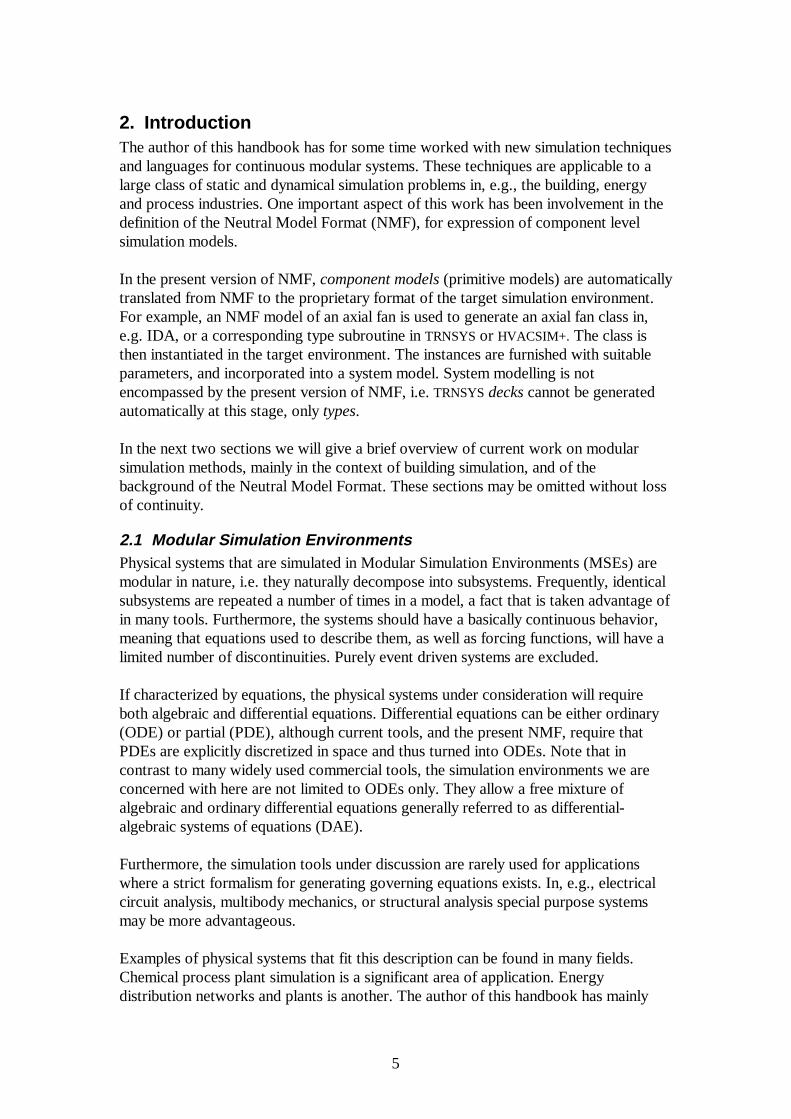
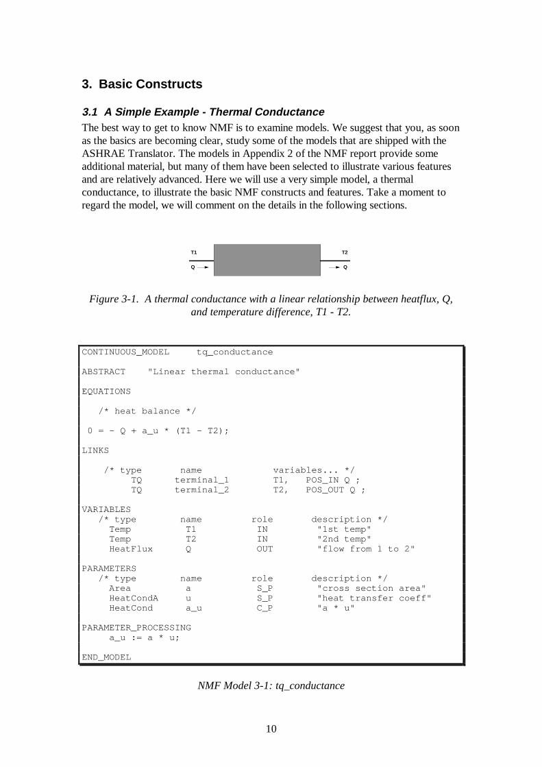
3.1 A Simple Example - Thermal ConductanceThe best way to get to know NMF is to examine models. We suggest that you, as soonas the basics are becoming clear, study some of the models that are shipped with theASHRAE Translator. The models in Appendix 2 of the NMF report provide someadditional material, but many of them have been selected to illustrate various featuresand are relatively advanced. Here we will use a very simple model, a thermalconductance, to illustrate the basic NMF constructs and features. Take a moment toregard the model, we will comment on the details in the following sections.
T1
Q
T2
Q
Figure 3-1. A thermal conductance with a linear relationship between heatflux, Q,and temperature difference, T1 - T2.
CONTINUOUS_MODEL tq_conductance
ABSTRACT "Linear thermal conductance"
EQUATIONS
/* heat balance */
0 = - Q + a_u * (T1 - T2);
LINKS
/* type name variables... */ TQ terminal_1 T1, POS_IN Q ; TQ terminal_2 T2, POS_OUT Q ;
VARIABLES /* type name role description */ Temp T1 IN "1st temp" Temp T2 IN "2nd temp" HeatFlux Q OUT "flow from 1 to 2"
PARAMETERS /* type name role description */ Area a S_P "cross section area" HeatCondA u S_P "heat transfer coeff" HeatCond a_u C_P "a * u"
PARAMETER_PROCESSING a_u := a * u;
END_MODEL
NMF Model 3-1: tq_conductance
11
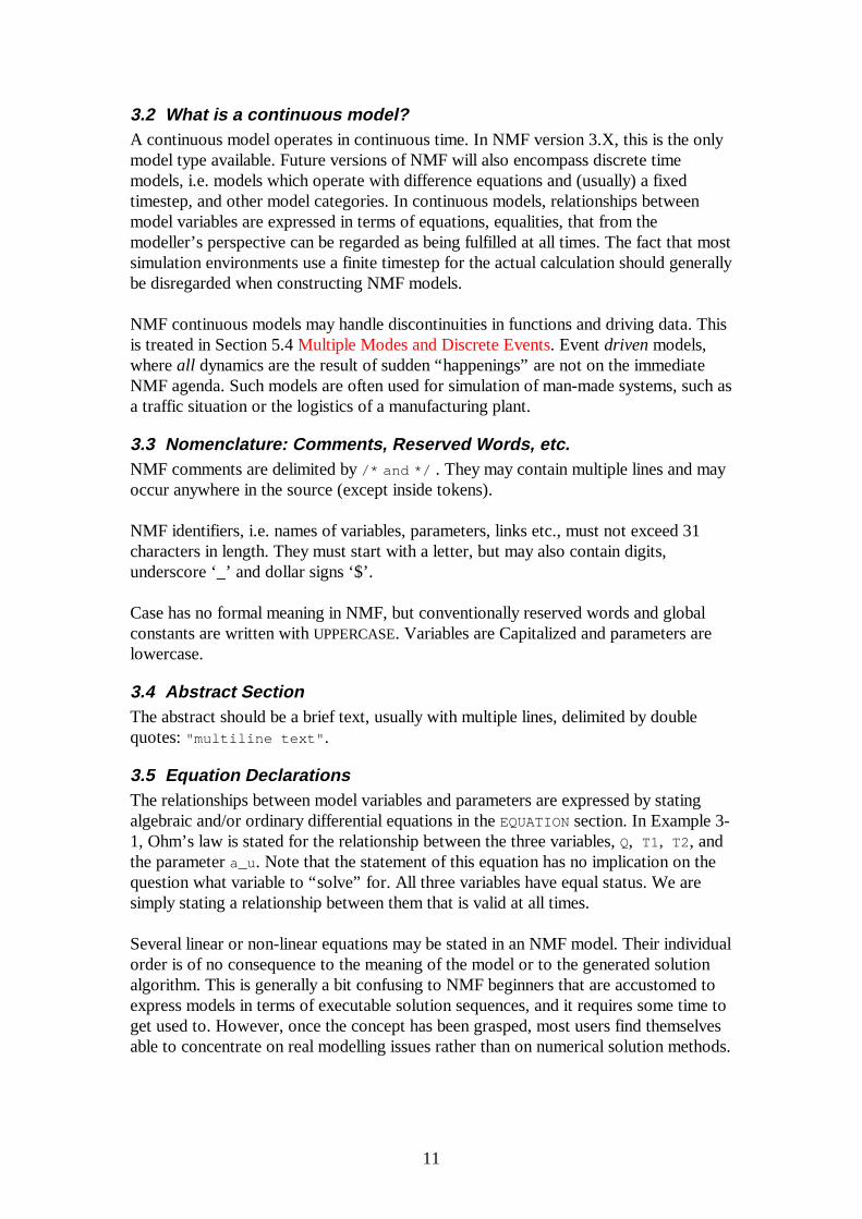
3.2 What is a continuous model?A continuous model operates in continuous time. In NMF version 3.X, this is the onlymodel type available. Future versions of NMF will also encompass discrete timemodels, i.e. models which operate with difference equations and (usually) a fixedtimestep, and other model categories. In continuous models, relationships betweenmodel variables are expressed in terms of equations, equalities, that from themodeller’s perspective can be regarded as being fulfilled at all times. The fact that mostsimulation environments use a finite timestep for the actual calculation should generallybe disregarded when constructing NMF models.
NMF continuous models may handle discontinuities in functions and driving data. Thisis treated in Section 5.4 Multiple Modes and Discrete Events. Event driven models,where all dynamics are the result of sudden “happenings” are not on the immediateNMF agenda. Such models are often used for simulation of man-made systems, such asa traffic situation or the logistics of a manufacturing plant.
3.3 Nomenclature: Comments, Reserved Words, etc.NMF comments are delimited by /* and */ . They may contain multiple lines and mayoccur anywhere in the source (except inside tokens).
NMF identifiers, i.e. names of variables, parameters, links etc., must not exceed 31characters in length. They must start with a letter, but may also contain digits,underscore ‘_’ and dollar signs ‘$’.
Case has no formal meaning in NMF, but conventionally reserved words and globalconstants are written with UPPERCASE. Variables are Capitalized and parameters arelowercase.
3.4 Abstract SectionThe abstract should be a brief text, usually with multiple lines, delimited by doublequotes: "multiline text" .
3.5 Equation DeclarationsThe relationships between model variables and parameters are expressed by statingalgebraic and/or ordinary differential equations in the EQUATION section. In Example 3-1, Ohm’s law is stated for the relationship between the three variables, Q, T1 , T2 , andthe parameter a_u . Note that the statement of this equation has no implication on thequestion what variable to “solve” for. All three variables have equal status. We aresimply stating a relationship between them that is valid at all times.
Several linear or non-linear equations may be stated in an NMF model. Their individualorder is of no consequence to the meaning of the model or to the generated solutionalgorithm. This is generally a bit confusing to NMF beginners that are accustomed toexpress models in terms of executable solution sequences, and it requires some time toget used to. However, once the concept has been grasped, most users find themselvesable to concentrate on real modelling issues rather than on numerical solution methods.
12
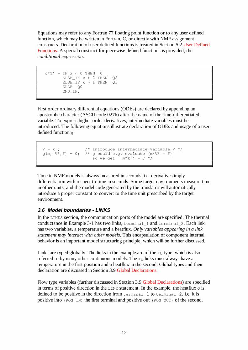
Equations may refer to any Fortran 77 floating point function or to any user definedfunction, which may be written in Fortran, C, or directly with NMF assignmentconstructs. Declaration of user defined functions is treated in Section 5.2 User DefinedFunctions. A special construct for piecewise defined functions is provided, theconditional expression:
c*T’ = IF x < 0 THEN 0 ELSE_IF x > 2 THEN Q2 ELSE_IF x > 1 THEN Q1 ELSE Q0 END_IF;
First order ordinary differential equations (ODEs) are declared by appending anapostrophe character (ASCII code 027h) after the name of the time-differentiatedvariable. To express higher order derivatives, intermediate variables must beintroduced. The following equations illustrate declaration of ODEs and usage of a userdefined function g:
V = X’; /* introduce intermediate variable V */ g(m, V’,F) = 0; /* g could e.g. evaluate (m*V’ - F) so we get m*X’’ = F */
Time in NMF models is always measured in seconds, i.e. derivatives implydifferentiation with respect to time in seconds. Some target environments measure timein other units, and the model code generated by the translator will automaticallyintroduce a proper constant to convert to the time unit prescribed by the targetenvironment.
3.6 Model boundaries - LINKSIn the LINKS section, the communication ports of the model are specified. The thermalconductance in Example 3-1 has two links, terminal_1 and terminal_2 . Each linkhas two variables, a temperature and a heatflux. Only variables appearing in a linkstatement may interact with other models. This encapsulation of component internalbehavior is an important model structuring principle, which will be further discussed.
Links are typed globally. The links in the example are of the TQ type, which is alsoreferred to by many other continuous models. The TQ links must always have atemperature in the first position and a heatflux in the second. Global types and theirdeclaration are discussed in Section 3.9 Global Declarations.
Flow type variables (further discussed in Section 3.9 Global Declarations) are specifiedin terms of positive direction in the LINK statement. In the example, the heatflux Q isdefined to be positive in the direction from terminal _1 to terminal _2 , i.e. it ispositive into (POS_IN) the first terminal and positive out (POS_OUT) of the second.
13
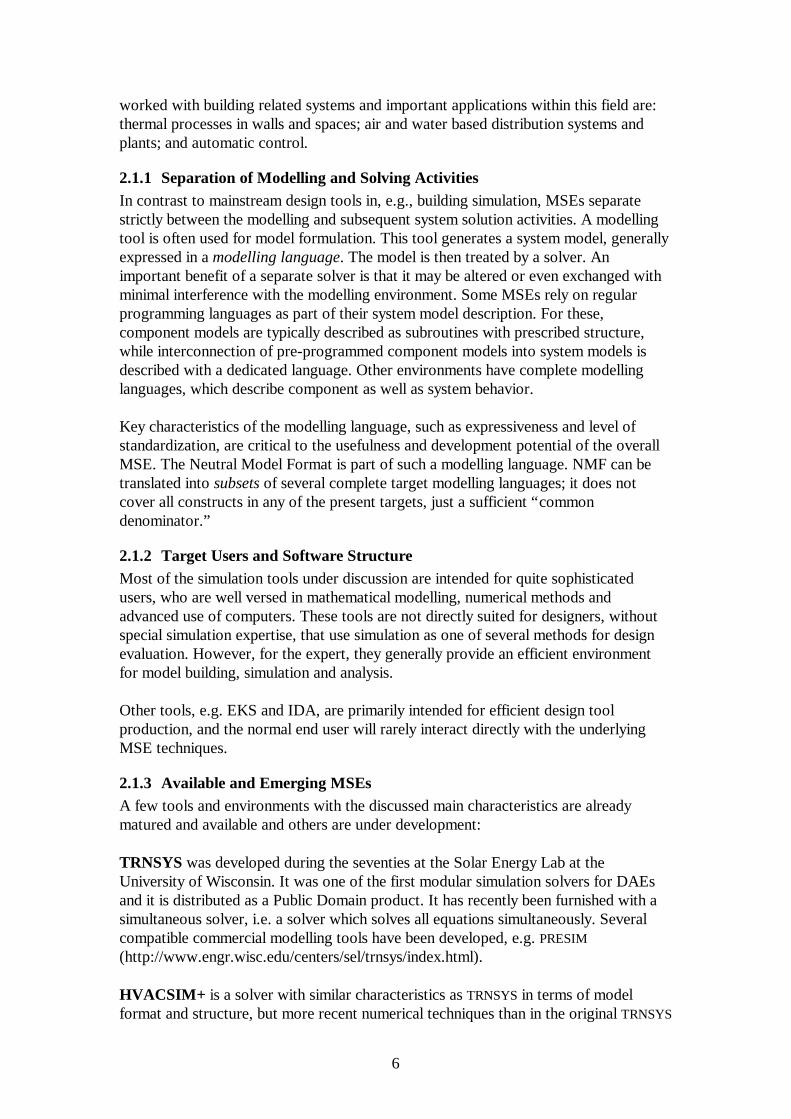
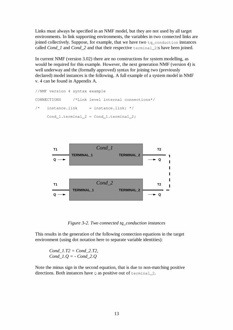
Links must always be specified in an NMF model, but they are not used by all targetenvironments. In link supporting environments, the variables in two connected links arejoined collectively. Suppose, for example, that we have two tq_conduction instancescalled Cond_1 and Cond_2 and that their respective terminal_2 :s have been joined.
In current NMF (version 3.02) there are no constructions for system modelling, aswould be required for this example. However, the next generation NMF (version 4) iswell underway and the (formally approved) syntax for joining two (previouslydeclared) model instances is the following. A full example of a system model in NMFv. 4 can be found in Appendix A.
//NMF version 4 syntax example
CONNECTIONS /*Link level internal connections*/
/* instance.link = instance.link; */
Cond_1.terminal_2 = Cond_1.terminal_2;
T1
Q
T2
Q
Cond_2
T1
Q
T2
Q
Cond_1TERMINAL_1
TERMINAL_1
TERMINAL_2
TERMINAL_2
Figure 3-2. Two connected tq_conduction instances
This results in the generation of the following connection equations in the targetenvironment (using dot notation here to separate variable identities):
Cond_1.T2 = Cond_2.T2,Cond_1.Q = - Cond_2.Q
Note the minus sign in the second equation, that is due to non-matching positivedirections. Both instances have Q as positive out of terminal_2 .
14
3.7 Variable and Parameter DeclarationsVariables and parameters are explicitly declared in an NMF model. Parameters arequantities that remain constant throughout every simulation. Each quantity, a variableor parameter, must be declared in four respects:
3.7.1 TypeSimilarly as for links, variables and parameters, are globally typed. As an alternative,they may be declared GENERIC, which roughly means that they are compatible with anyother type.
3.7.2 NameThe local name for the quantity.
3.7.3 RoleVariables are divided into four different roles: IN , OUT, LOC, and A_S. The two latterconcern assignment modelling and are treated in Section 5.3 NMF VariableAssignments. A modeller is required to specify one possible selection of given (IN ) andcalculated (OUT) variables, and the number of OUT-variables must be equal to thenumber of equations in the model. The selection should be made to maximize modelrobustness. The reasons for requiring this information are discussed below.
Parameters can be either supplied, S_P, or computed, C_P. The former are givenexplicitly by the user, while computed parameters are calculated in the PARAMETER
PROCESSING section, which is executed once, prior to the actual simulation. Both S_P
and C_P parameters may occur in equations in the EQUATION section.
3.7.4 DescriptionA descriptive string must be given for each variable or parameter. It cannot exceed 80characters. Each white space between words is counted as a single character, even if itin fact contains several tab, newline, or space characters.
In addition to this, a quantity may optionally be given a default value and an interval inwhich the model is valid. These declarations are described further in the NMF report,Sections 4.2.4 - 5.
3.7.5 IN/OUT DiscussionThe explicit selection of given (IN ) and calculated (OUT) variables for a model mayseem to contradict the principles of equation-based input-output free modelling thatform the basis of NMF. However, for environments where models are packaged assubroutines, with inputs and outputs, a selection is needed. The IN /OUT labels onvariables in the NMF source code is one way to signal the desired partitioning. TheASHRAE translator to TRNSYS and HVACSIM+ utilizes this method.
Consequently, one reason for including this information is that maximal compatibility isattained with the large number of existing input-output oriented environments. Usingthe IN/OUT information, it is always possible to translate an NMF model into theseenvironments directly, without adding anything extra. It should also be observed thatmost models in the libraries of such environments exist in a single input-output version.
15
For many application domains, only a few models are duplicated with different input-output structures to attain connectivity. A further discussion of these issues can befound in Section 3.1 of the NMF report. The issue is also discussed in Exercise 1.
The more fundamental argument for the IN-OUT partitioning is that different selectionshave different robustness properties, and this is taken advantage of in someenvironments. The given selection should be a “good inverse” for the whole model (inthe matrix sense). An extreme example is a limited proportional controller, where it ispossible to calculate the in signal from the out signal in the proportional band, but notin any saturated state. See also Section 3.5 of the NMF Report.
3.7.6 Order of Declared QuantitiesThe order of quantity declarations does not influence the mathematical meaning of amodel. However, an NMF implementation is allowed to use the order for otherpurposes. Frequently, the order of variables and parameters in the generated code isidentical to that of the NMF source. In the ASHRAE Translator, for example, theorder of declarations is used to generate an order for the input, output, and parametervectors of the TYPE subroutines. (See the Generated Code Section of the user’smanual.)
3.8 Parameter ProcessingIn the PARAMETER_PROCESSING section, computed parameters (C_P) are calculatedfrom supplied ditto (S_P). The code is executed once at the start of a simulation. Alimited range of algorithmic constructs such as IF <condition> THEN ... ELSE
... END_IF are available. There are no potentially endless iteration constructs such asWHILE <condition> DO .
Standard and user-defined functions may be referred to, as in the EQUATION section.Standard functions include all Fortran 77 floating point operations, and a routine forsignaling errors NMF_ERROR, which takes any number of strings and expressions asarguments. NMF_ERROR and other special functions are discussed in Section 4.3 of theNMF Report.
IF Re < 2500 THEN CALL NMF_ERROR ("Laminar flow, Reynolds number = ", Re)END_IF;
3.8.1 Restriction on Repeated AssignmentsCompared to regular programming, one important difference applies. In NMF, aquantity may not be assigned to repeatedly. It may or may not be assigned to -depending on the thread of execution - but once assigned, it is illegal to update thevariable again.
The reason for this limitation is that it should, for the benefit of pure equation basedenvironments, always be possible to interpret NMF assignments as if they wereequations. The limitation also enables a range of symbolic processing constructs thatwould otherwise be out of reach.
16
One consequence of this restriction is illustrated by the following example.
FOR i = 1, n /* NOT permitted */ help := a [i ] - b [i ] ; /* help assigned repeatedly */ c [i ] := IF help < 0 THEN 0 ELSE help**2 END_IF ;END_FOR ;
Two alternative ways to respect the restriction are shown:
FOR i = 1, n c [i ] := IF a [i ] - b [i ] < 0 THEN 0 ELSE (a [i ] - b [i ])**2 END_IF ;END_FOR ;
FOR i = 1, n help [i ] := a [i ] - b [i ] ; c [i ] := IF help [i ] < 0 THEN 0 ELSE help [i ]**2 END_IF ;END_FOR ;
Another aspect of the restriction relates to conditional assignments. Here, theinterpretation of the restriction is less obvious.
In the present version of NMF, it is formally permitted to lexically assign a variable inall of a series of mutually exclusive IF THEN ... END_IF constructs. Thispossibility will most likely be removed in future versions, and it is thereforerecommended to assign a parameter only within a single, possibly complex, conditionalconstruct.
This construction, for example, is presently formally allowed but not recommended:
IF test <= 1 THEN a := 2END_IF;...<other assignments>...IF test > 3 THEN a := 4END_IF;

17
A recommended construction is:
IF test <= 1 THEN a := 2ELSE_IF test > 3 THEN a := 4END_IF;
Note that in both these constructions, a will not always be defined.
3.9 Global DeclarationsThe basic idea with NMF is to provide a way to exchange models between developers.One thing that makes model exchange difficult today is that people naturally makedifferent choices in rather trivial matters such as selection of units and variables. Someprefer to use e.g. enthalpy to get compact equations, others pick temperature to gainengineering appeal. The modest ambition of NMF is to recommend some choices, toattain standardization on a voluntary basis, but without limiting the freedom of theindividual modeller.
Global declarations include quantity types, ordered lists of quantity types called linktypes, and global constants. Global declarations is sometimes also called foundation. Abasic list of recommended global declarations will be issued regularly by the NMFCommittee. A user may add to or change this list as necessary. An excerpt from thepresent global.nmf file is:
QUANTITY_TYPES
/* type name unit kind */
Area "m2" CROSS Control "dimless" CROSS Density "kg/m3" CROSS Factor "dimless" CROSS Force "N" CROSS HeatCap "J/(K)" CROSS HeatCapA "J/(K m2)" CROSS HeatCapM "J/(kg K)" CROSS HeatCond "W/K" THRU HeatCondL "W/(m K)" THRU HeatCondA "W/(m2 K)" THRU HeatFlux "W" THRU HeatFlux_k "kW" THRU Length "m" CROSS MassFlow "kg/s" THRU Pressure "Pa" CROSS Temp "Deg-C" CROSS
LINK_TYPES
/* type name variable types... */
/* generic (arbitrary, arbitrary,...) implicitly defined */
Q (HeatFlux) T (Temp) TQ (Temp, HeatFlux) PMT (Pressure, MassFlow, Temp)
18
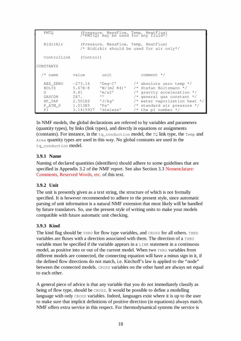
PMTQ (Pressure, MassFlow, Temp, HeatFlux) /*PMT(Q) may be used for any fluid*/
BidirAir (Pressure, MassFlow, Temp, HeatFlux) /* BidirAir should be used for air only*/
ControlLink (Control)
CONSTANTS
/* name value unit comment */
ABS_ZERO -273.16 "Deg-C" /* absolute zero temp */ BOLTZ 5.67E-8 "W/(m2 K4)" /* Stefan Boltzmann */ G 9.81 "m/s2" /* gravity acceleration */ GASCON 287. "" /* general gas constant */ HF_VAP 2.501E6 "J/kg" /* water vaporization heat */ P_ATM_0 1.013E5 "Pa" /* standard air pressure */ PI 3.1415927 "dimless" /* the pi number */
In NMF models, the global declarations are referred to by variables and parameters(quantity types), by links (link types), and directly in equations or assignments(constants). For instance, in the tq_conduction model, the TQ link type, the Temp andArea quantity types are used in this way. No global constants are used in thetq_conduction model.
3.9.1 NameNaming of declared quantities (identifiers) should adhere to some guidelines that arespecified in Appendix 3.2 of the NMF report. See also Section 3.3 Nomenclature:Comments, Reserved Words, etc. of this text.
3.9.2 UnitThe unit is presently given as a text string, the structure of which is not formallyspecified. It is however recommended to adhere to the present style, since automaticparsing of unit information is a natural NMF extension that most likely will be handledby future translators. So, use the present style of writing units to make your modelscompatible with future automatic unit checking.
3.9.3 KindThe kind flag should be THRU for flow type variables, and CROSS for all others. THRU
variables are fluxes with a direction associated with them. The direction of a THRU
variable must be specified if the variable appears in a LINK statement in a continuousmodel, as positive into or out of the current model. When two THRU variables fromdifferent models are connected, the connecting equation will have a minus sign in it, ifthe defined flow directions do not match, i.e. Kirchoff’s law is applied to the “node”between the connected models. CROSS variables on the other hand are always set equalto each other.
A general piece of advice is that any variable that you do not immediately classify asbeing of flow type, should be CROSS. It would be possible to define a modellinglanguage with only CROSS variables. Indeed, languages exist where it is up to the userto make sure that implicit definitions of positive direction (in equations) always match.NMF offers extra service in this respect. For thermodynamical systems the service is
19
very valuable, for some other applications it is less useful. (See for example Exercise1.)
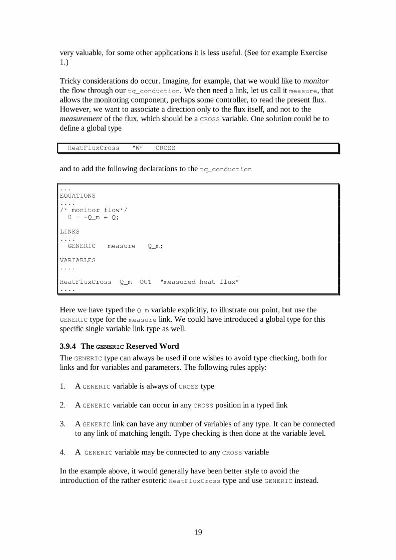
Tricky considerations do occur. Imagine, for example, that we would like to monitorthe flow through our tq_conduction . We then need a link, let us call it measure , thatallows the monitoring component, perhaps some controller, to read the present flux.However, we want to associate a direction only to the flux itself, and not to themeasurement of the flux, which should be a CROSS variable. One solution could be todefine a global type
HeatFluxCross “W” CROSS
and to add the following declarations to the tq_conduction
...EQUATIONS..../* monitor flow*/ 0 = -Q_m + Q;
LINKS.... GENERIC measure Q_m;
VARIABLES....
HeatFluxCross Q_m OUT “measured heat flux”....
Here we have typed the Q_m variable explicitly, to illustrate our point, but use theGENERIC type for the measure link. We could have introduced a global type for thisspecific single variable link type as well.
3.9.4 The GENERIC Reserved Word
The GENERIC type can always be used if one wishes to avoid type checking, both forlinks and for variables and parameters. The following rules apply:
1. A GENERIC variable is always of CROSS type
2. A GENERIC variable can occur in any CROSS position in a typed link
3. A GENERIC link can have any number of variables of any type. It can be connectedto any link of matching length. Type checking is then done at the variable level.
4. A GENERIC variable may be connected to any CROSS variable
In the example above, it would generally have been better style to avoid theintroduction of the rather esoteric HeatFluxCross type and use GENERIC instead.
20
3.10 File StructureNMF does not specify the precise structure for source files. Global declarations musthowever be kept together in a single file, possibly decomposed into several includefiles. Some implementations have each model in a single file, others have all modelsthat belong to the same (informal) model family in a single file. The ASHRAEtranslator can effectively handle both these file organizations.
21
4. Modelling GuidelinesIn this section we will attempt to convey some qualitative aspects of the art of NMFmodelling. Experience has been gained from several significant simulation projects, andsome general conclusions regarding modelling methodology can be drawn.
The set of basic constructs that were presented in the previous section represent thecore that is needed for simple models. In this section we will base the discussion onthese basic constructs. The more advanced constructs that will be treated later will notaffect the validity of the modelling guidelines presented here.
We will introduce some general guidelines in the first sections and then illustrate themwith an example regarding pressure-flow modelling with models which allow massflowto change direction.
4.1 Thinking Equation Declaration - Not Assignment ProgrammingThe difference between an algorithmic description of a model and an equationdescription is frequently misunderstood. NMF is sometimes erroneously thought of asa proposed standard for algorithmic descriptions. Let us look for a moment at thedifference between algorithms and equations.
4.1.1 Algorithmic ModelsAn algorithm is used to describe a computation procedure, a step by step recipe onhow to get from input to output. Some important characteristics of algorithms are:
1. Variables are defined as either input, output, or local
2. A variable receives it’s value by assignment of the value of some computableexpression, possibly involving the variable itself
3. The same variable may be assigned to repeatedly
4. Variables are often repeatedly assigned in loops, which are executed until somecriterion is met, i.e. not an easily predictable number of times.
4.1.2 Equation ModelsEquation models state a mathematical relationship between variables. The followingcharacteristics apply:
1. If the number of variables, k, exceeds the number of linearly independent equations,N, then k - N variables may be given as input, and the remainder, N, can usually besolved for analytically or numerically.
2. A variable should be thought of as having a value at all times; the equations may bemore or less satisfied depending on current variable values. If anything is to becalled output of the equation model, it is the value of the residuals in each equation.
3. The order of equations and the arrangement of terms in equations is irrelevant to themeaning of the model.
22
4.1.3 DiscussionThe main advantage of expressing models in terms of equations rather than asalgorithms is that an equation model generally can be automatically converted into analgorithm, whereas the opposite is only possible in a small number of cases.Furthermore, several algorithms with, for example, different input-outputconfigurations can be generated from the same equation model. Equation models alsolend themselves to other types of symbolic processing, which is of great importance tosimulation, for example automatic differentiation.
Many people with programming experience tend to look for the same concepts andtools for NMF work as they are accustomed to. Some things are certainly common forall types of formal coding work, but one must be aware of the differences. Someexamples are:
1. It is generally misleading to think of a continuous model as a concept similar to asubroutine or a function in a regular language. A better mental picture is to think ofthe model as a class definition in an object oriented language. A class which can beinstantiated multiple times, each with its own private set of data, and each with theability to say how well it’s equations are fulfilled.
2. There is far less need for sophisticated data structures in the NMF domain than in aregular language.
3. NMF model definitions tend to be reused in various configurations and by otherusers to a greater extent than what is generally the case for subroutine and classdefinitions.
4. NMF modelling is more work intensive than most other regular programming, interms of produced code per time unit.
4.2 Finding Component Model BoundariesThe first task to tackle in developing a library of NMF models for a specific applicationis to divide the system to be simulated into separate component models. The real art ofNMF modelling lies in finding the proper boundaries for component models. Manyphysical systems have a natural decomposition into component models, that one shouldtry to mimic in the modelling. Others, such as a thermal zone model, require muchmore careful planning in order to achieve a good structure with versatile componentpieces. Some things to consider are:
1. Identify “flow circuits” in the system, where a common link type can be used tocommunicate between individual components. Try to keep the number of link typesto a minimum. Examples of such circuits in a building simulation are: the ductsystem, the water pipe system, heat transfer between objects (using, for example,the TQ link type).
2. Define component boundaries that minimize the data shared between components,i.e. try as far as possible to avoid cases when two models need the same variable orparameter.
23
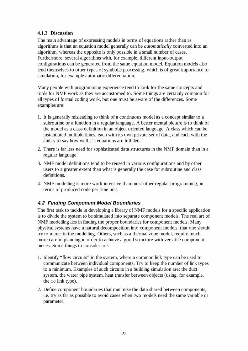
3. There is no optimal size of a component model, large models are sometimes morepractical, small usually more versatile. For most solvers, large models are morecomputationally efficient.
Take a look at some component model libraries that are shipped with the translator toget a feel for model architecture. Some libraries have been translated from othersources and they may not be ideal from an NMF architectural point of view. Mostmodels contain advanced constructs, as will be presented in the next section, but thearchitectural concepts remain the same.
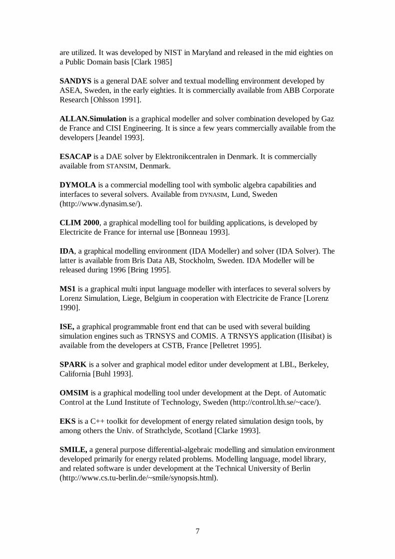
4.3 The Right Number of Equations in Each ModelIt is sometimes difficult to decide what equations go where. Two general guidelinesapply:
1. Try to make models as self-contained as possible.
T1 T2 T3
NOT RECOMMENDED!
Figure 4-1. Dashed boundaries are a possible subdivision of an RC-network intoNMF component models with only a single variable, T, on the links. The
disadvantages are that the resistor (or conductor) parameters are duplicated inneighboring models, and the equation for ohm’s law is similarly duplicated.
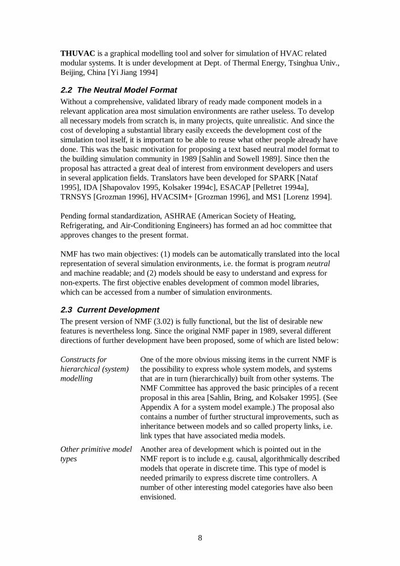
T1 T2 T3
RECOMMENDED!
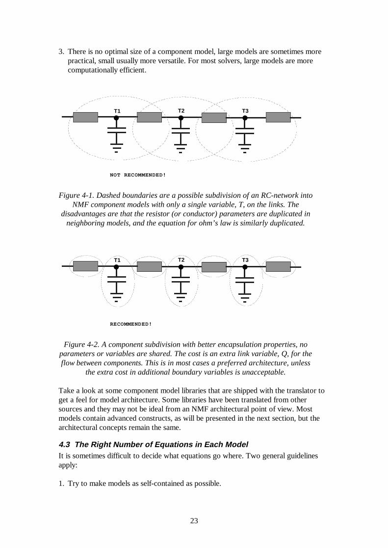
Figure 4-2. A component subdivision with better encapsulation properties, noparameters or variables are shared. The cost is an extra link variable, Q, for theflow between components. This is in most cases a preferred architecture, unless
the extra cost in additional boundary variables is unacceptable.
24
2. Say everything there is to say about a component, but only once. Never state thesame equation twice.
One must rely on “engineering intuition” here, but this seldom leads to any significantproblems in practice.
4.4 A Useful Special Case - Bi-directional FlowWe will now turn to an example rooted in a real life NMF application, multizoneairflow.
The Multizone Air-Exchange (MAE) models constitute an example of a componentfamily that have been developed primarily for IDA, but that should be useful in otherenvironments as well. However, these models are rather numerically demanding, and itis not reasonable to expect that they will perform satisfactorily with any solver. Theissue of limitations in the matching between models and solvers will be discussedfurther in Section 4.7 Target environment capabilities.
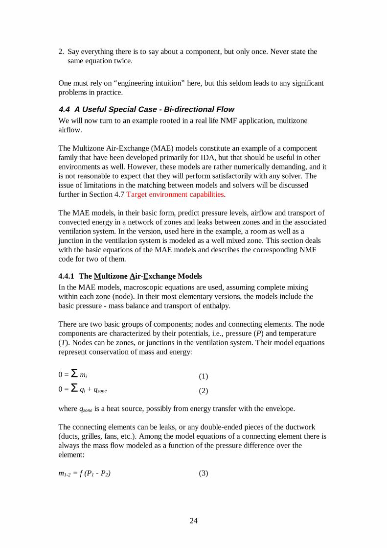
The MAE models, in their basic form, predict pressure levels, airflow and transport ofconvected energy in a network of zones and leaks between zones and in the associatedventilation system. In the version, used here in the example, a room as well as ajunction in the ventilation system is modeled as a well mixed zone. This section dealswith the basic equations of the MAE models and describes the corresponding NMFcode for two of them.
4.4.1 The Multizone Air-E xchange ModelsIn the MAE models, macroscopic equations are used, assuming complete mixingwithin each zone (node). In their most elementary versions, the models include thebasic pressure - mass balance and transport of enthalpy.
There are two basic groups of components; nodes and connecting elements. The nodecomponents are characterized by their potentials, i.e., pressure (P) and temperature(T). Nodes can be zones, or junctions in the ventilation system. Their model equationsrepresent conservation of mass and energy:
0 = Σ mi (1)
0 = Σ qi + qzone (2)
where qzone is a heat source, possibly from energy transfer with the envelope.
The connecting elements can be leaks, or any double-ended pieces of the ductwork(ducts, grilles, fans, etc.). Among the model equations of a connecting element there isalways the mass flow modeled as a function of the pressure difference over theelement:
m1-2 = f (P1 - P2) (3)
25
In the example of this text power law equations are used for the pressure - flowrelation. For a leak this implies:
c(∆p)n, ∆p > 0f(∆p) = (4)
-c(-∆p)n, ∆p < 0
where n is a coefficient between 0.5 and 1.0, depending on flow type, and c is a“conductivity” coefficient.
Heat (enthalpy) transport through a connecting element is convected by the mass flow:
cpT1m1-2, m1-2 > 0q1-2 = (5)
cpT2m1-2, m1-2 < 0
where T1 and T2 are the temperatures of the nodes connected by the element.
This type of modular approach makes it easy to replace individual component modelsas long as the interface variables between models are the same. Thus, it is possible torefine on the MAE models by replacing the above equations by more detailed ones.
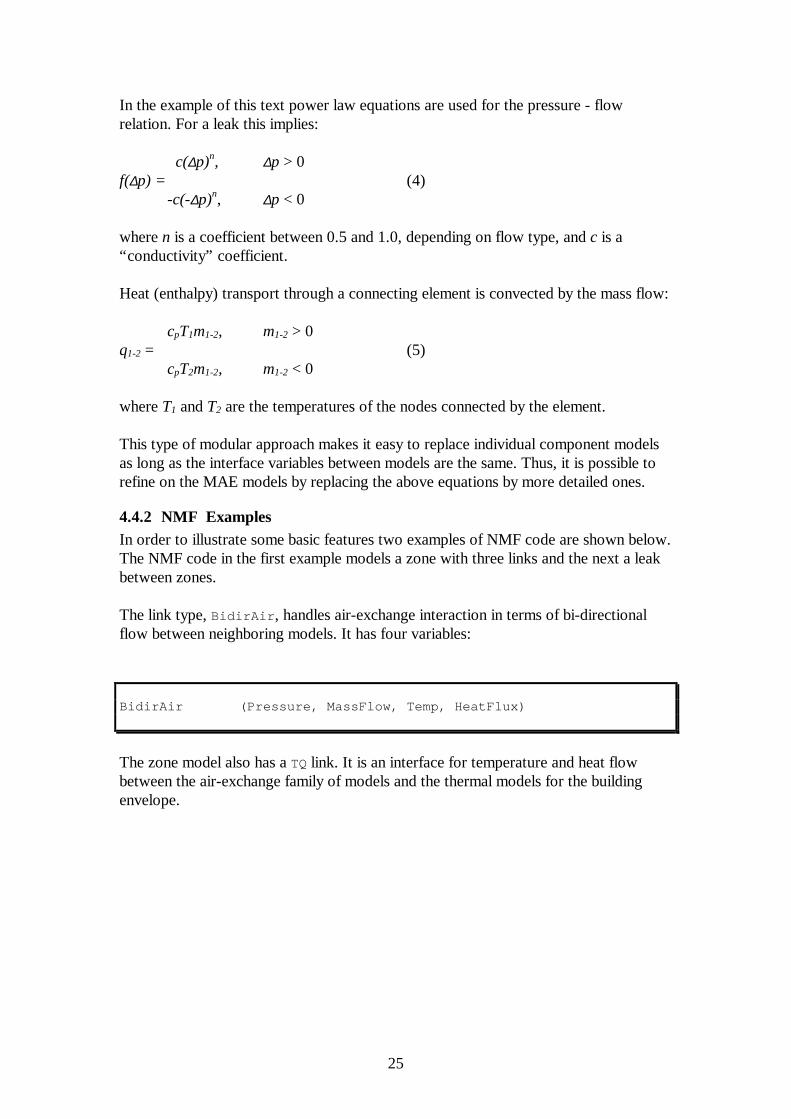
4.4.2 NMF ExamplesIn order to illustrate some basic features two examples of NMF code are shown below.The NMF code in the first example models a zone with three links and the next a leakbetween zones.
The link type, BidirAir , handles air-exchange interaction in terms of bi-directionalflow between neighboring models. It has four variables:
BidirAir (Pressure, MassFlow, Temp, HeatFlux)
The zone model also has a TQ link. It is an interface for temperature and heat flowbetween the air-exchange family of models and the thermal models for the buildingenvelope.
26
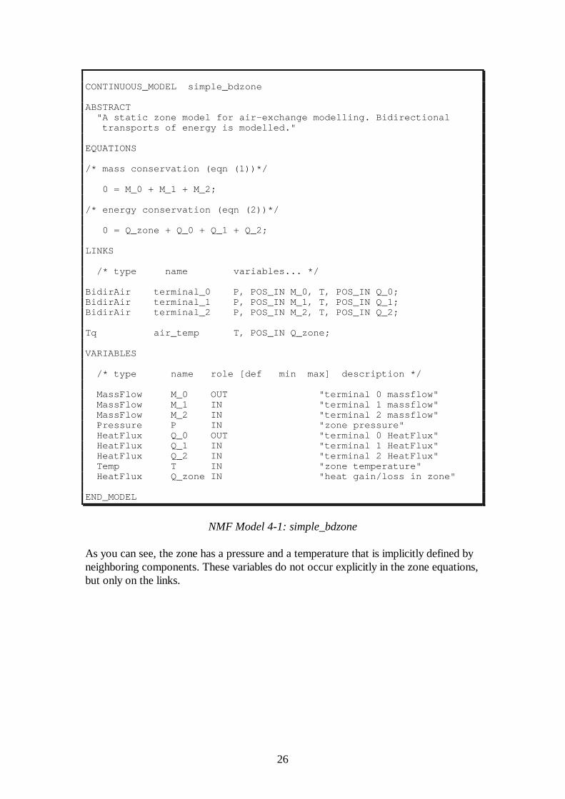
CONTINUOUS_MODEL simple_bdzone
ABSTRACT "A static zone model for air-exchange modelling. Bidirectional transports of energy is modelled."
EQUATIONS
/* mass conservation (eqn (1))*/
0 = M_0 + M_1 + M_2;
/* energy conservation (eqn (2))*/
0 = Q_zone + Q_0 + Q_1 + Q_2;
LINKS
/* type name variables... */
BidirAir terminal_0 P, POS_IN M_0, T, POS_IN Q_0;BidirAir terminal_1 P, POS_IN M_1, T, POS_IN Q_1;BidirAir terminal_2 P, POS_IN M_2, T, POS_IN Q_2;
Tq air_temp T, POS_IN Q_zone;
VARIABLES
/* type name role [def min max] description */
MassFlow M_0 OUT "terminal 0 massflow" MassFlow M_1 IN "terminal 1 massflow" MassFlow M_2 IN "terminal 2 massflow" Pressure P IN "zone pressure" HeatFlux Q_0 OUT "terminal 0 HeatFlux" HeatFlux Q_1 IN "terminal 1 HeatFlux" HeatFlux Q_2 IN "terminal 2 HeatFlux" Temp T IN "zone temperature" HeatFlux Q_zone IN "heat gain/loss in zone"
END_MODEL
NMF Model 4-1: simple_bdzone
As you can see, the zone has a pressure and a temperature that is implicitly defined byneighboring components. These variables do not occur explicitly in the zone equations,but only on the links.

27
CONTINUOUS_MODEL simple_bdleak
ABSTRACT "A simplified powerlaw leak model w/ bidirectionaltransports tempered air."
EQUATIONS
/*driving pressure difference*/
Dp = P1 - P2;
/* powerlaw massflow equation (eqns (3) and (4))*/
M = IF Dp > 0 THEN c * Dp**n ELSE -c * (-Dp)**n END_IF ;
/* convected heat through leak (eqn (5))*/
Q = IF M > 0.0 THEN cp * T1 * M ELSE cp * T2 * M END_IF ;
LINKS
/* type name variables... */
BidirAir terminal_1 P1, POS_IN M, T1, POS_IN QBidirAir terminal_2 P2, POS_OUT M, T2, POS_OUT Q;
VARIABLES
/* type name role def min max description */
MassFlow M OUT 0 -BIG BIG "massflow through leak"Pressure P1 IN 1 -BIG BIG "terminal 1 pressure"Pressure P2 IN 2 -BIG BIG "terminal 2 pressure"Temp T1 IN 20 ABS_ZERO BIG "Temperature of neighbor 1"Temp T2 IN 20 ABS_ZERO BIG "Temperature of neighbor 2"HeatFlux Q OUT 0 -BIG BIG "heat moved by massflow"Pressure Dp OUT "effective pressure diff."
PARAMETERS
/* type name role def min max description */Generic c S_P 1 0 BIG "powerlaw coeff. [kg/(s Pa**n)]"Generic n S_P .5 .5 1.0 "powerlaw exponent [dimless]"HeatCapM cp S_P 1006 .5E3 3E3 "air cp"END_MODEL
NMF Model 4-2: simple_bdleak
These two models can be combined into arbitrary networks. The connection rules arethat two zones always must be connected via one or more leaks. Leaks may beconnected in series. These rules are not formalized in the models, but are implied bythe way the equations have been formulated. In future versions of NMF, connectionrules like these may well be formalized.
28
Key to the understanding of these models is the fact that the pressure and temperaturethat appear in the leak model are valid for the neighboring components. P and T of thezone model become computable since they occur in equations in the leak model.
A new concept in the leak model is the default, minimum, and maximum values thatmay be defined for each variable or parameter. Most real models have such explicitlimits coded.
The zone and leak models have the BidirAir link allowing for bi-directional flow. Letus model a ventilation component with unidirectional flow as well, since bi-directionalflow modelling in the ventilation system may be too costly (more variables andequations) for some applications.
For unidirectional modelling we need only three link variables: pressure, massflow andtemperature, and, generally, only a single equation (3). The three-variable link type iscalled PMT. Simple link types are generally named after the variables in them, whereascomplex ones have other descriptive names.
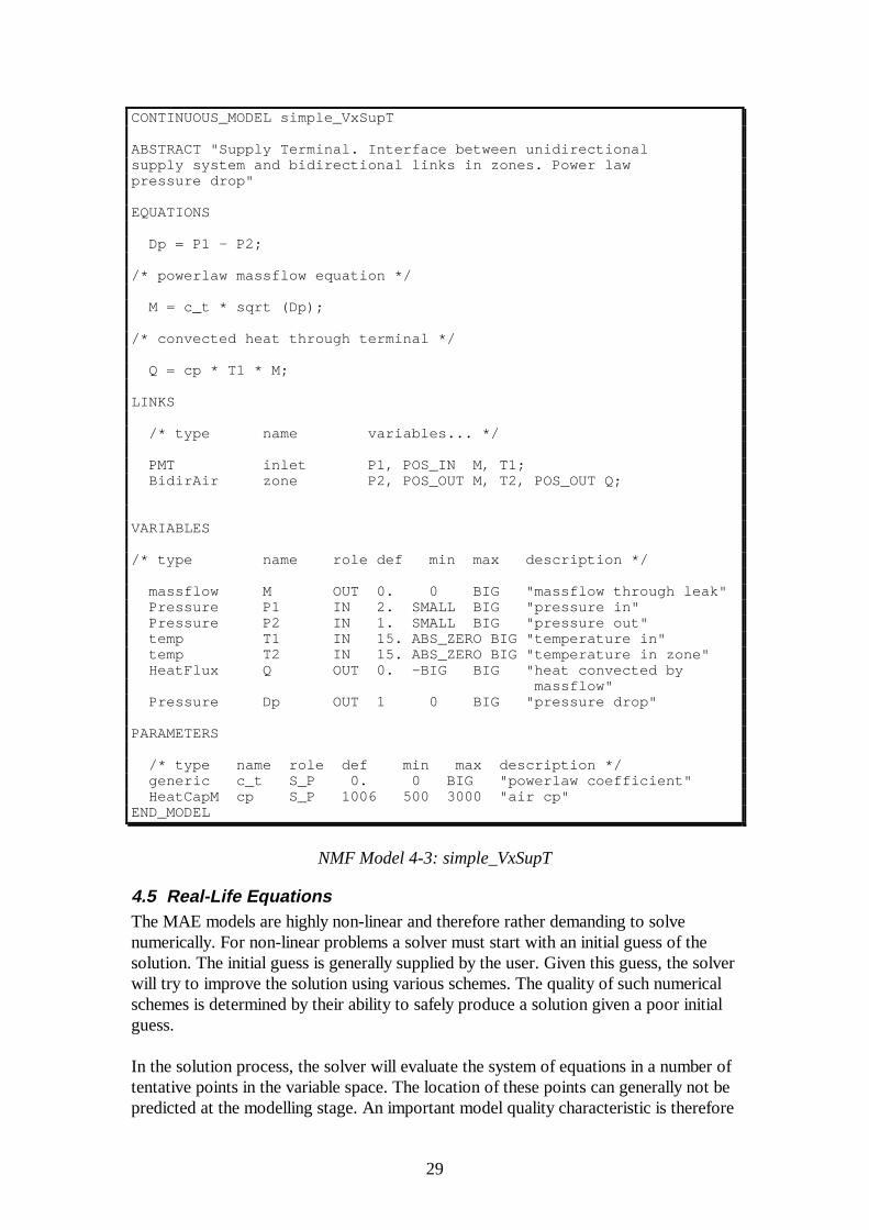
We will present a single unidirectional model, a supply terminal model,simple_VxSupT , that acts as interface between zone models, with BidirAir links,and the supply side of the ventilation system, with PMT links. Consequently, thesimple_VxSupT model has one link of each kind. Although only uni-directional flow isallowed, it still needs two equations (in addition to the calculation of dp) since there isa BidirAir link present.
29
CONTINUOUS_MODEL simple_VxSupT
ABSTRACT "Supply Terminal. Interface between unidirectionalsupply system and bidirectional links in zones. Power lawpressure drop"
EQUATIONS
Dp = P1 - P2;
/* powerlaw massflow equation */
M = c_t * sqrt (Dp);
/* convected heat through terminal */
Q = cp * T1 * M;
LINKS
/* type name variables... */
PMT inlet P1, POS_IN M, T1; BidirAir zone P2, POS_OUT M, T2, POS_OUT Q;
VARIABLES
/* type name role def min max description */
massflow M OUT 0. 0 BIG "massflow through leak" Pressure P1 IN 2. SMALL BIG "pressure in" Pressure P2 IN 1. SMALL BIG "pressure out" temp T1 IN 15. ABS_ZERO BIG "temperature in" temp T2 IN 15. ABS_ZERO BIG "temperature in zone" HeatFlux Q OUT 0. -BIG BIG "heat convected by
massflow" Pressure Dp OUT 1 0 BIG "pressure drop"
PARAMETERS
/* type name role def min max description */ generic c_t S_P 0. 0 BIG "powerlaw coefficient" HeatCapM cp S_P 1006 500 3000 "air cp"END_MODEL
NMF Model 4-3: simple_VxSupT
4.5 Real-Life EquationsThe MAE models are highly non-linear and therefore rather demanding to solvenumerically. For non-linear problems a solver must start with an initial guess of thesolution. The initial guess is generally supplied by the user. Given this guess, the solverwill try to improve the solution using various schemes. The quality of such numericalschemes is determined by their ability to safely produce a solution given a poor initialguess.
In the solution process, the solver will evaluate the system of equations in a number oftentative points in the variable space. The location of these points can generally not bepredicted at the modelling stage. An important model quality characteristic is therefore
30
that models permit evaluation also in odd variable combinations, without riskingdivision by zero or that the derivative of an equation with respect to its variablesbecomes infinite. Most solvers try to estimate such derivatives in the solution process.
The simple MAE models that we have just discussed, will work well for good qualityinitial guesses, if the massflows in the solution process stay away from zero. Oneproblem is that the derivative of equation (4) with respect to ∆p becomes infinitearound zero, and since the purpose of the models is to predict bi-directional flow, theyshould be robust for evaluation in the neighborhood of zero massflow.
Solution ideas to these types of difficulties can often be obtained from the physics ofthe problem. In our case, for a small enough flow through an opening, there will be aswitch to laminar flow, with a corresponding linear relationship between flow andpressure. If equation (4) is augmented with a linear section around zero, we should beable to avoid the problem:
c(∆p)n, ∆p > ∆p0
f(∆p) = c0∆p, abs(∆p) < ∆p0 (4b)-c(-∆p)n, ∆p < -∆p0
where the parameter ∆p0 could be selected to be smaller than any interesting pressuredifference to resolve. c0 can be computed to give a continuous transition between thedifferent regimes of equation (4b).
Explicit isolation of singularities like we have just seen, and equations that are possibleto evaluate in any “strange” regime are characteristics of a good quality model. Aclassical pitfall is when a polynomial is used to interpolate between measured points onsome curve, e.g. a fan curve. The polynomial fit may work reasonably well within theoperating regime of the fan, but can be completely off in other areas, even having thewrong sign. A solver is much more likely to converge if the fan curve has a reasonableslope outside of the (physical) operating regime as well.
4.5.1 User-Independent Initial GuessesAnother problem with the MAE models, as with any non-linear model, is that theyrequire a reasonable initial guess to be provided in order to converge safely. This maybe acceptable for some applications, and equally unacceptable for others. If forexample, a few thousand non-linear equations are solved, it becomes both difficult andtedious to provide any non-trivial initial guess.
NMF provides a way around this problem by a system function called LINEARIZE . If asolver supports this feature, a call to LINEARIZE will return true in the first fewiterations. The model can then detect this and behave linearly or close to linearly in thiscase, and thus provide a user-independent and reasonable initial state, since mostsolvers will solve a linear system in one iteration independent of the starting point.
The LINEARIZE function can also be invoked in several steps, to introduce non-linearities in a model successively. Study the specification in Section 4.3.3 in the NMFreport.

31
Equations (3) - (5) in the “real life” MAE leak model bdleak , with both isolation ofthe singularity around zero and a LINEARIZE call, look like:
/* powerlaw massflow equation */
M = IF LINEARIZE (1) THEN c * Dp ELSE_IF abs (Dp) < dp0 THEN c0 * Dp ELSE_IF Dp > 0 THEN c * Dp**n ELSE -c * (-Dp)**n END_IF BAD_INVERSES () ;
/* convected heat through leak*/
Q = IF LINEARIZE (1) THEN (T1 - T2) / 2 ELSE_IF M > 0.0 THEN cp * T1 * M ELSE cp * T2 * M END_IF GOOD_INVERSES (Q) ;
The BAD_ and GOOD_INVERSES declarations are discussed in the Section 4.6Declaration of Bad Inverses.
The linearized model for the heatflux Q deserves some comment. It makes no effort todepict reality. However, if similar constructs are used in other components, thetemperatures reached in the linear stage will be averages between boundarytemperatures. Given the weak coupling from temperature to pressure in normalventilation studies, this should mean realistic temperatures in most cases. Thus, thismodel will not aggravate the difficulties with the non-linear flow balance.
4.5.2 Additional Features of the Multizone Air Exchange Model FamilyIn the previous sections, exerpts and simplified versions of the MAE models have beenpresented. The full library is shipped with the ASHRAE NMF Translator. It is a goodreference example. The full models contain several language constructs that will bepresented in the section on Advanced Constructs. They also model some additionalphysics that has not yet been discussed:
Stack effect Driving forces due to temperature dependent density change aremodeled throughout the library. Zones are assumed to be well mixed -no temperature gradients are modeled. An oddity in the design is worthmentioning: The models utleak , utsupt , and utexht are used as“boundary objects” to the environment. They all have the outside airpressure at ground level on their outside link. The pressure at thelevel of the actual device is calculated internally.
Contaminantfraction
In addition to the transport of heat with the air, a fraction of somearbitrary substance is also modeled throughout the circuit. Zones havesource terms for fraction production, and all models take properaccount of the transport and conservation of the fraction.
32
The MAE models are discussed in more detail in some separate reports [Sahlin, Bring1993] [Sahlin, Bring 1995].
4.6 Declaration of Bad InversesNMF equations are frequently treated symbolically to generate, for example, variousinverses. When the ASHRAE Translator generates Fortran code for TRNSYS andHVACSIM+, equations are whenever possible solved symbolically to calculate OUT fromIN variables. Only in the case when no complete symbolic solution is found, does thetranslator rely on numerical methods. In most cases, the translator is able toautomatically determine what symbolic operations can be done without risk ofintroducing potential errors (generally division by zero). The user can also explicitlydeclare potentially hazardous inverses of equations, by adding a comma delimited listof BAD_INVERSES to an equation before the terminating semicolon. This feature isnaturally most important for symbolic solvers that are unable to make good decisionsin this respect on their own.
The user can similarly specify GOOD_INVERSES of an equation. This is more interestingfor a modern symbolic solver, since this way the user can add knowledge about themodel that is difficult to deduce automatically.
4.7 Target environment capabilitiesNMF tries to overcome many of the trivial problems in transferring models betweendifferent simulation environments. There are however fundamental environmentdifferences that prevent some models to be implemented in certain targetenvironments.
The MAE family is a good example of a rather demanding set of models that areunlikely to converge in, for example, a sequential solver such as the traditional TRNSYS
solver. The new simultaneous TRNSYS solver (v. 14) should be able to handle the MAEmodels.
It would be unreasonable to require that any NMF model can be solved in any targetenvironment, since this would, not only in practice be impossible to ensure, but alsolimit the incentive for solver improvement that simplified model transfer is likely tobring.
A smaller, more practical problem is that most present NMF models have beenimplemented primarily for use with input-output free solvers, and that the presentselection of IN and OUT variables may prove inadequate for practical work in otherenvironments. Hopefully, the quality of the libraries will be improved in this respect, asthey are more widely used in input-output environments, such as TRNSYS v. 13, andHVACSIM+.
Another similar problem is the different conventions regarding units and variablechoices that have evolved in the dedicated model libraries around existingenvironments. It is an impossible mission for NMF to try to be compatible with all ofthese, and the only feasible solution seems to be the evolution of a new separate NMFbased culture in this respect.

33
5. Advanced ConstructsThe basic constructs that we have presented so far are sufficient for small modellibraries that are mainly intended to illustrate the concept. Unfortunately, the academicdiscussion about modelling languages rarely goes beyond such simple examples.However, real-scale modelling puts entirely new requirements on the language. NMFhas a strong set of features that enable non-academic modelling. This side of thelanguage has been prioritized at the expense of other features, such as hierarchicalmodelling, and other types of structuring support, that are mainly needed for systemrather than component modelling. Basic system modelling features have been proposedand are now being refined and tested, but they are not discussed in this text.
5.1 Vectors and MatricesFew other modelling languages have working implementations of vector and matrixsupport. NMF is built to enable dynamic changes of field dimensions, i.e. aninstantiated NMF model can increase field dimensions interactively. This is very usefulfor a graphical modelling environment where models have, for example, a dynamicnumber of links. Take for instance the MAE zone model that was discussed in theprevious section. It happened to have three BidirAir links, but clearly this is nosacred number. In many applications one would need a larger number of links, and ininteractive modelling, one would like this number to be flexible. A morecomprehensive zone model is:
CONTINUOUS_MODEL less_simple_Bdzone
ABSTRACT "A static zone model for air-exchange modelling. Bidirectional transports of energy are modelled."
EQUATIONS
/* mass conservation */ 0 = M_0 + SUM i=1, n M[i] END_SUM BAD_INVERSES () ;
/* energy conservation */ 0 = Q_zone + Q_0 + SUM i=1, n Q[i] END_SUM BAD_INVERSES () ;
LINKS
/* type name variables... */
BidirAir terminal_0 P, POS_IN M_0, T, POS_IN Q_0;
FOR i = 1, n BidirAir terminal[i] P, POS_IN M[i], T, POS_IN Q[i]END_FOR ;
TQ air_temp T, POS_IN Q_zone;
VARIABLES
/* type name role [def [min max]] description */ MassFlow M_0 OUT "terminal 0 massflow" MassFlow M[n] IN "terminal i massflow"
34
Pressure P IN "zone pressure" HeatFlux Q_0 OUT "terminal 0 HeatFlux" HeatFlux Q[n] IN "terminal i HeatFlux" Temp T IN "zone temperature" HeatFlux Q_zone IN "heat gain/loss in zone"
MODEL_PARAMETERS
/* type name role [def min max] description */ INT n SMP 1 1 BIGINT "Number of links minus one"
END_MODEL
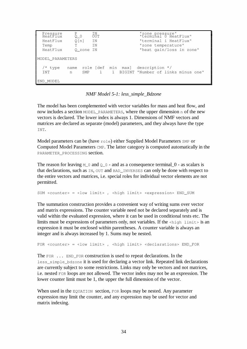
NMF Model 5-1: less_simple_Bdzone
The model has been complemented with vector variables for mass and heat flow, andnow includes a section MODEL_PARAMETERS, where the upper dimension n of the newvectors is declared. The lower index is always 1. Dimensions of NMF vectors andmatrices are declared as separate (model) parameters, and they always have the typeINT .
Model parameters can be (have role ) either Supplied Model Parameters SMP orComputed Model Parameters CMP. The latter category is computed automatically in thePARAMETER_PROCESSING section.
The reason for leaving M_0 and Q_0 - and as a consequence terminal_0 - as scalars isthat declarations, such as IN , OUT and BAD_INVERSES can only be done with respect tothe entire vectors and matrices, i.e. special roles for individual vector elements are notpermitted.
SUM <counter> = <low limit> , <high limit> <expression> END_SUM
The summation construction provides a convenient way of writing sums over vectorand matrix expressions. The counter variable need not be declared separately and isvalid within the evaluated expression, where it can be used in conditional tests etc. Thelimits must be expressions of parameters only, not variables. If the <high limit> is anexpression it must be enclosed within parentheses. A counter variable is always aninteger and is always increased by 1. Sums may be nested.
FOR <counter> = <low limit> , <high limit> <declarations> END_FOR
The FOR ... END_FOR construction is used to repeat declarations. In theless_simple_bdzone it is used for declaring a vector link. Repeated link declarationsare currently subject to some restrictions. Links may only be vectors and not matrices,i.e. nested FOR loops are not allowed. The vector index may not be an expression. Thelower counter limit must be 1, the upper the full dimension of the vector.
When used in the EQUATION section, FOR loops may be nested. Any parameterexpression may limit the counter, and any expression may be used for vector andmatrix indexing.
35
5.1.1 Model Parameter Declaration and ProcessingModel parameters are always positive scalar integers (type INT ). It is important toremember to declare the minimum value of the model parameter for which the model isvalid.
Computed model parameters (CMP) may be functions of supplied model parameters(SMP) ditto, not of regular parameters. They are computed by assignment in thePARAMETER_PROCESSING section.
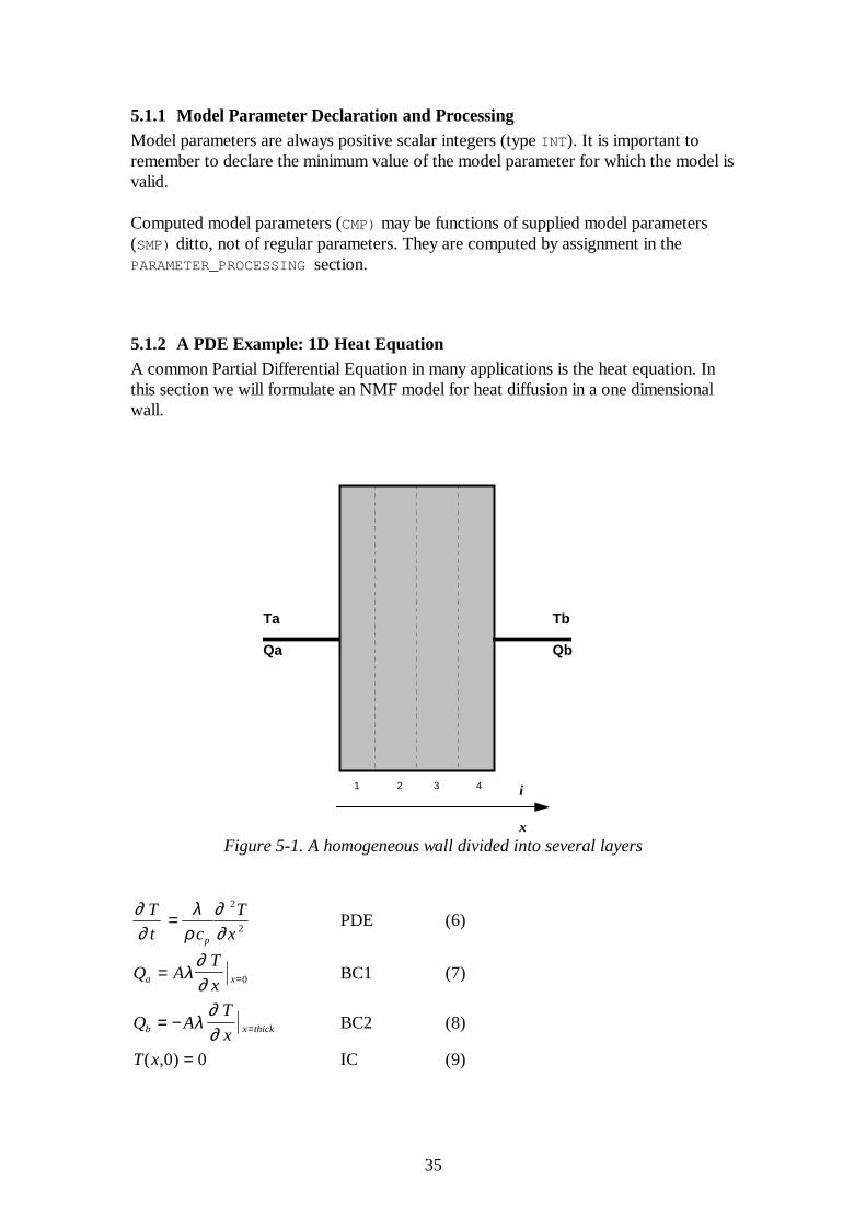
5.1.2 A PDE Example: 1D Heat EquationA common Partial Differential Equation in many applications is the heat equation. Inthis section we will formulate an NMF model for heat diffusion in a one dimensionalwall.
Ta
Qa
Tb
Qb
1 2 3 4 i
xFigure 5-1. A homogeneous wall divided into several layers
∂∂
λρ
∂∂
T
t c
T
xp
=2
2PDE (6)
Q AT
xa x= =λ∂∂ 0 BC1 (7)
Q AT
xb x thick= − =λ∂∂
BC2 (8)
T x( , )0 0= IC (9)
36
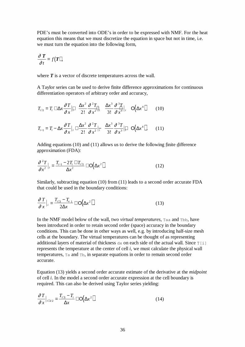
PDE’s must be converted into ODE’s in order to be expressed with NMF. For the heatequation this means that we must discretize the equation in space but not in time, i.e.we must turn the equation into the following form,
( )∂∂
TT
tf= ,
where T is a vector of discrete temperatures across the wall.
A Taylor series can be used to derive finite difference approximations for continuousdifferentiation operators of arbitrary order and accuracy,
( )T T xT
x
x T
x
x T
xxi i i i i+ = + + + +1
2 2
2
3 3
34
2 3∆ ∆ ∆ Ο ∆∂
∂∂∂
∂∂! !
(10)
( )T T xT
x
x T
x
x T
xxi i i i i− = − + − +1
2 2
2
3 3
34
2 3∆ ∆ ∆ Ο ∆∂
∂∂∂
∂∂! !
. (11)
Adding equations (10) and (11) allows us to derive the following finite differenceapproximation (FDA):
( )∂∂
2
21 1
222T
x
T T T
xxi
i i i= − + +− +
∆Ο ∆ . (12)
Similarly, subtracting equation (10) from (11) leads to a second order accurate FDAthat could be used in the boundary conditions:
( )∂∂
T
x
T T
xxi
i i=−
++ −1 1 2
2∆Ο ∆ . (13)
In the NMF model below of the wall, two virtual temperatures, Taa and Tbb, havebeen introduced in order to retain second order (space) accuracy in the boundaryconditions. This can be done in other ways as well, e.g. by introducing half-size meshcells at the boundary. The virtual temperatures can be thought of as representingadditional layers of material of thickness dx on each side of the actual wall. Since T[i]
represents the temperature at the center of cell i, we must calculate the physical walltemperatures, Ta and Tb, in separate equations in order to remain second orderaccurate.
Equation (13) yields a second order accurate estimate of the derivative at the midpointof cell i. In the model a second order accurate expression at the cell boundary isrequired. This can also be derived using Taylor series yielding:
( )∂∂
T
x
T T
xxi
i i+
+=−
+1 21 2
/ ∆Ο ∆ . (14)
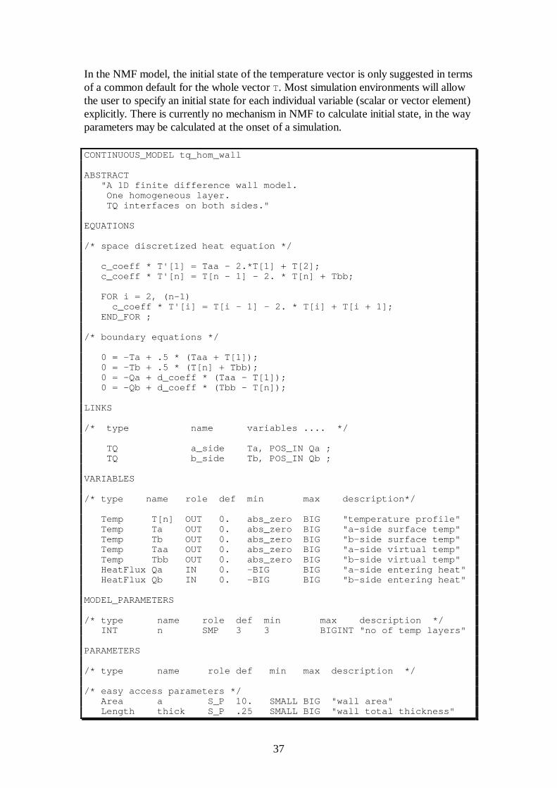
37
In the NMF model, the initial state of the temperature vector is only suggested in termsof a common default for the whole vector T. Most simulation environments will allowthe user to specify an initial state for each individual variable (scalar or vector element)explicitly. There is currently no mechanism in NMF to calculate initial state, in the wayparameters may be calculated at the onset of a simulation.
CONTINUOUS_MODEL tq_hom_wall
ABSTRACT "A 1D finite difference wall model. One homogeneous layer. TQ interfaces on both sides."
EQUATIONS
/* space discretized heat equation */
c_coeff * T'[1] = Taa - 2.*T[1] + T[2]; c_coeff * T'[n] = T[n - 1] - 2. * T[n] + Tbb;
FOR i = 2, (n-1) c_coeff * T'[i] = T[i - 1] - 2. * T[i] + T[i + 1]; END_FOR ;
/* boundary equations */
0 = -Ta + .5 * (Taa + T[1]); 0 = -Tb + .5 * (T[n] + Tbb); 0 = -Qa + d_coeff * (Taa - T[1]); 0 = -Qb + d_coeff * (Tbb - T[n]);
LINKS
/* type name variables .... */
TQ a_side Ta, POS_IN Qa ; TQ b_side Tb, POS_IN Qb ;
VARIABLES
/* type name role def min max description*/
Temp T[n] OUT 0. abs_zero BIG "temperature profile" Temp Ta OUT 0. abs_zero BIG "a-side surface temp" Temp Tb OUT 0. abs_zero BIG "b-side surface temp" Temp Taa OUT 0. abs_zero BIG "a-side virtual temp" Temp Tbb OUT 0. abs_zero BIG "b-side virtual temp" HeatFlux Qa IN 0. -BIG BIG "a-side entering heat" HeatFlux Qb IN 0. -BIG BIG "b-side entering heat"
MODEL_PARAMETERS
/* type name role def min max description */ INT n SMP 3 3 BIGINT "no of temp layers"
PARAMETERS
/* type name role def min max description */
/* easy access parameters */ Area a S_P 10. SMALL BIG "wall area" Length thick S_P .25 SMALL BIG "wall total thickness"
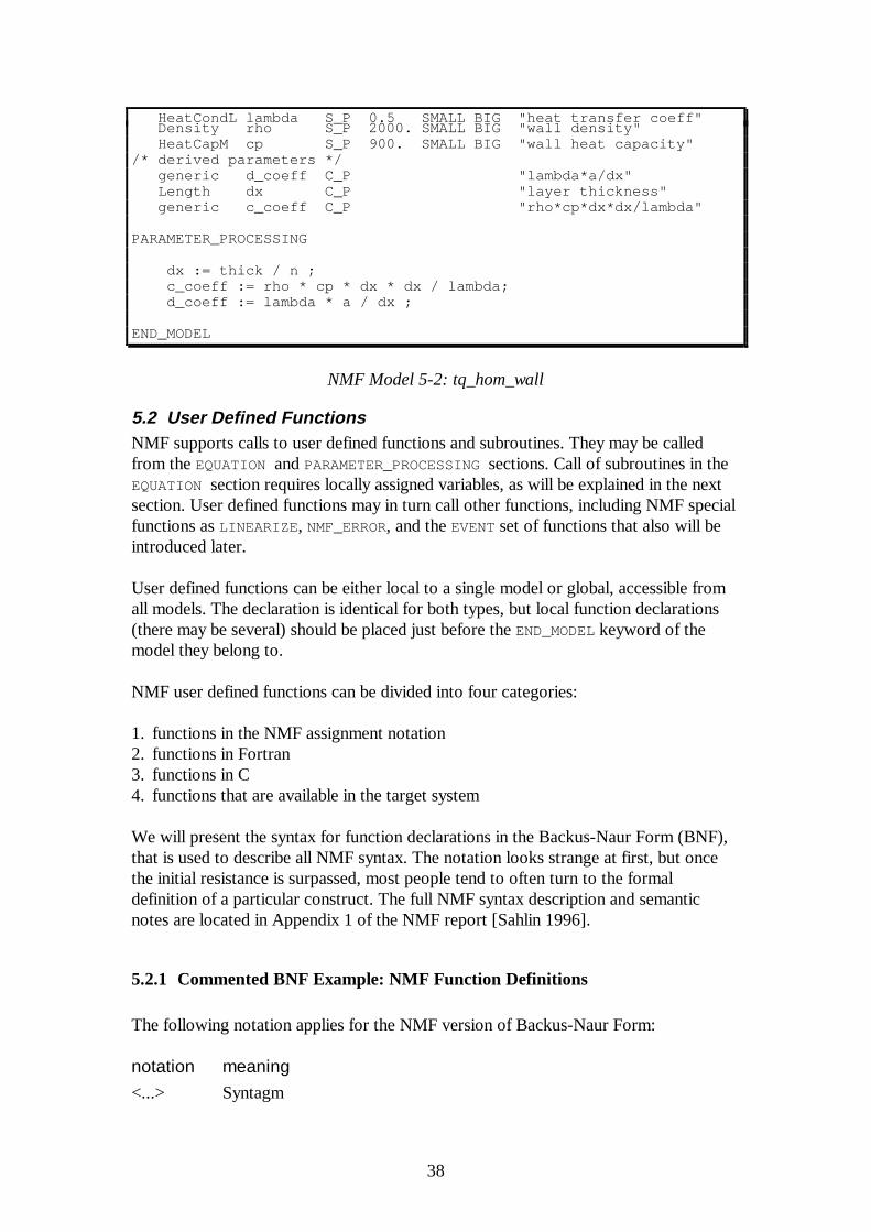
38
HeatCondL lambda S_P 0.5 SMALL BIG "heat transfer coeff" Density rho S_P 2000. SMALL BIG "wall density" HeatCapM cp S_P 900. SMALL BIG "wall heat capacity"/* derived parameters */ generic d_coeff C_P "lambda*a/dx" Length dx C_P "layer thickness" generic c_coeff C_P "rho*cp*dx*dx/lambda"
PARAMETER_PROCESSING
dx := thick / n ; c_coeff := rho * cp * dx * dx / lambda; d_coeff := lambda * a / dx ;
END_MODEL
NMF Model 5-2: tq_hom_wall
5.2 User Defined FunctionsNMF supports calls to user defined functions and subroutines. They may be calledfrom the EQUATION and PARAMETER_PROCESSING sections. Call of subroutines in theEQUATION section requires locally assigned variables, as will be explained in the nextsection. User defined functions may in turn call other functions, including NMF specialfunctions as LINEARIZE , NMF_ERROR, and the EVENT set of functions that also will beintroduced later.
User defined functions can be either local to a single model or global, accessible fromall models. The declaration is identical for both types, but local function declarations(there may be several) should be placed just before the END_MODEL keyword of themodel they belong to.
NMF user defined functions can be divided into four categories:
1. functions in the NMF assignment notation2. functions in Fortran3. functions in C4. functions that are available in the target system
We will present the syntax for function declarations in the Backus-Naur Form (BNF),that is used to describe all NMF syntax. The notation looks strange at first, but oncethe initial resistance is surpassed, most people tend to often turn to the formaldefinition of a particular construct. The full NMF syntax description and semanticnotes are located in Appendix 1 of the NMF report [Sahlin 1996].
5.2.1 Commented BNF Example: NMF Function Definitions
The following notation applies for the NMF version of Backus-Naur Form:
notation meaning
<...> Syntagm
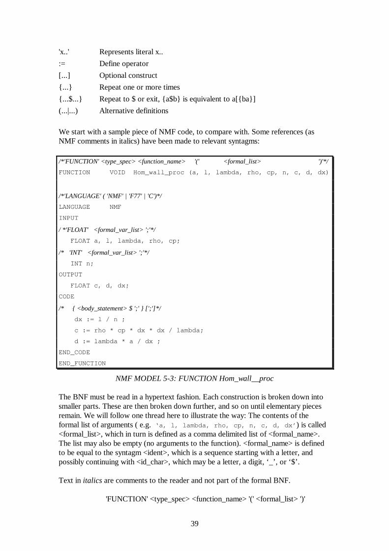
39
'x..' Represents literal x..
:= Define operator
[...] Optional construct
{...} Repeat one or more times
{...$...} Repeat to $ or exit, {a$b} is equivalent to a[{ba}]
(...|...) Alternative definitions
We start with a sample piece of NMF code, to compare with. Some references (asNMF comments in italics) have been made to relevant syntagms:
/*'FUNCTION' <type_spec> <function_name> '(' <formal_list> ')'*/
FUNCTION VOID Hom_wall_proc (a, l, lambda, rho, cp, n, c, d, dx)
/*'LANGUAGE' ( 'NMF' | 'F77' | 'C')*/
LANGUAGE NMF
INPUT
/ *'FLOAT' <formal_var_list> ';'*/
FLOAT a, l, lambda, rho, cp;
/* 'INT' <formal_var_list> ';'*/
INT n;
OUTPUT
FLOAT c, d, dx;
CODE
/* { <body_statement> $ ';' } [';']*/
dx := l / n ;
c := rho * cp * dx * dx / lambda;
d := lambda * a / dx ;
END_CODE
END_FUNCTION
NMF MODEL 5-3: FUNCTION Hom_wall__proc
The BNF must be read in a hypertext fashion. Each construction is broken down intosmaller parts. These are then broken down further, and so on until elementary piecesremain. We will follow one thread here to illustrate the way: The contents of theformal list of arguments ( e.g. ‘a, l, lambda, rho, cp, n, c, d, dx’ ) is called<formal_list>, which in turn is defined as a comma delimited list of <formal_name>.The list may also be empty (no arguments to the function). <formal_name> is definedto be equal to the syntagm <ident>, which is a sequence starting with a letter, andpossibly continuing with <id_char>, which may be a letter, a digit, ‘_’, or ‘$’.
Text in italics are comments to the reader and not part of the formal BNF.
'FUNCTION' <type_spec> <function_name> '(' <formal_list> ')'
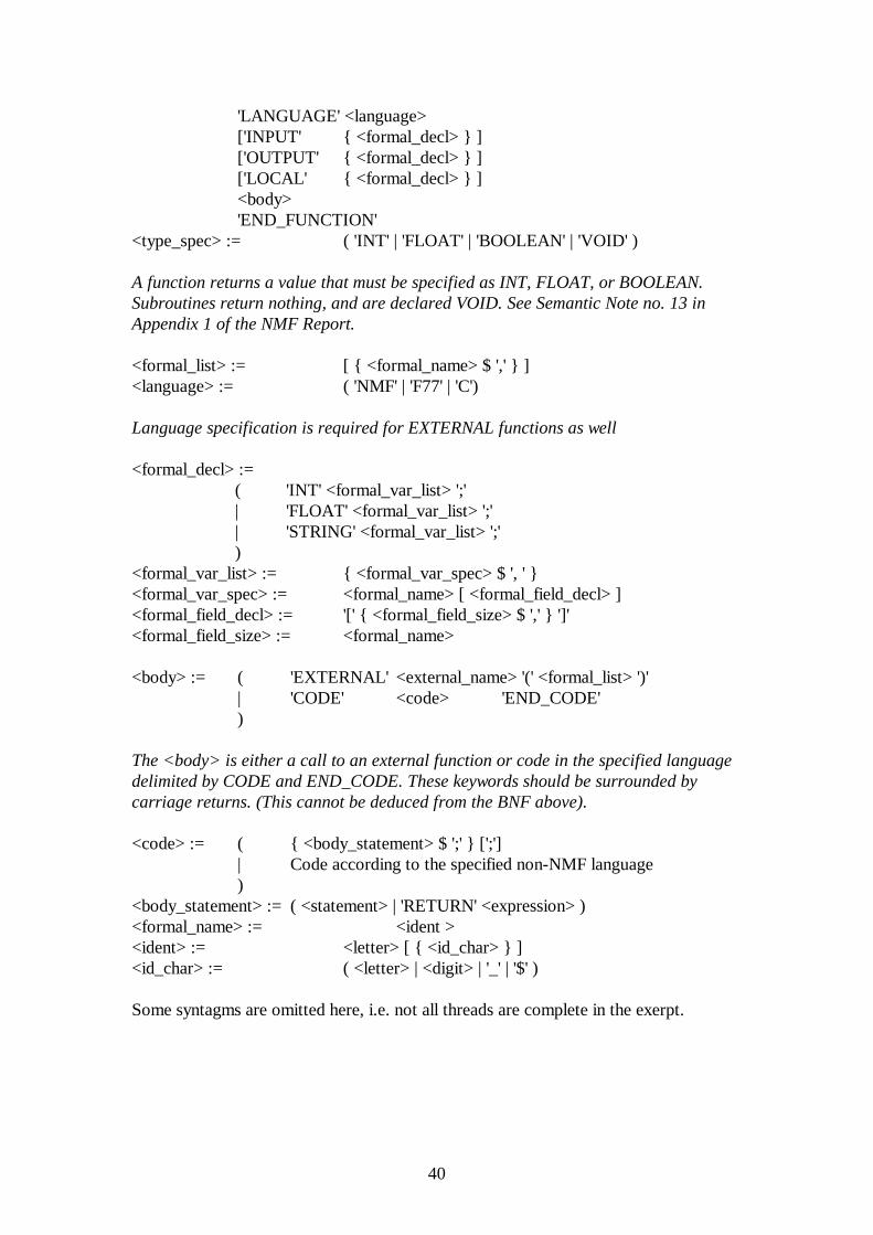
40
'LANGUAGE' <language>['INPUT' { <formal_decl> } ]['OUTPUT' { <formal_decl> } ]['LOCAL' { <formal_decl> } ]<body>'END_FUNCTION'
<type_spec> := ( 'INT' | 'FLOAT' | 'BOOLEAN' | 'VOID' )
A function returns a value that must be specified as INT, FLOAT, or BOOLEAN.Subroutines return nothing, and are declared VOID. See Semantic Note no. 13 inAppendix 1 of the NMF Report.
<formal_list> := [ { <formal_name> $ ',' } ]<language> := ( 'NMF' | 'F77' | 'C')
Language specification is required for EXTERNAL functions as well
<formal_decl> :=( 'INT' <formal_var_list> ';'| 'FLOAT' <formal_var_list> ';'| 'STRING' <formal_var_list> ';')
<formal_var_list> := { <formal_var_spec> $ ', ' }<formal_var_spec> := <formal_name> [ <formal_field_decl> ]<formal_field_decl> := '[' { <formal_field_size> $ ',' } ']'<formal_field_size> := <formal_name>
<body> := ( 'EXTERNAL' <external_name> '(' <formal_list> ')'| 'CODE' <code> 'END_CODE')
The <body> is either a call to an external function or code in the specified languagedelimited by CODE and END_CODE. These keywords should be surrounded bycarriage returns. (This cannot be deduced from the BNF above).
<code> := ( { <body_statement> $ ';' } [';']| Code according to the specified non-NMF language)
<body_statement> := ( <statement> | 'RETURN' <expression> )<formal_name> := <ident ><ident> := <letter> [ { <id_char> } ]<id_char> := ( <letter> | <digit> | '_' | '$' )
Some syntagms are omitted here, i.e. not all threads are complete in the exerpt.
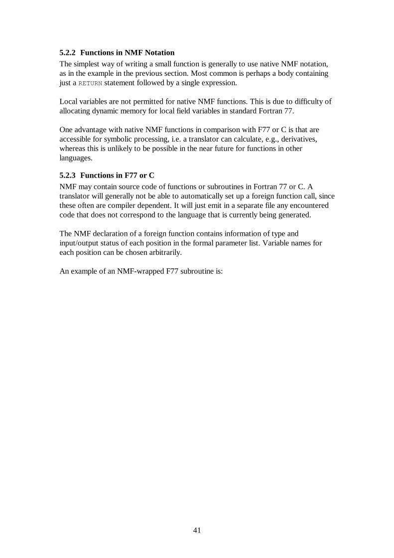
41
5.2.2 Functions in NMF NotationThe simplest way of writing a small function is generally to use native NMF notation,as in the example in the previous section. Most common is perhaps a body containingjust a RETURN statement followed by a single expression.
Local variables are not permitted for native NMF functions. This is due to difficulty ofallocating dynamic memory for local field variables in standard Fortran 77.
One advantage with native NMF functions in comparison with F77 or C is that areaccessible for symbolic processing, i.e. a translator can calculate, e.g., derivatives,whereas this is unlikely to be possible in the near future for functions in otherlanguages.
5.2.3 Functions in F77 or CNMF may contain source code of functions or subroutines in Fortran 77 or C. Atranslator will generally not be able to automatically set up a foreign function call, sincethese often are compiler dependent. It will just emit in a separate file any encounteredcode that does not correspond to the language that is currently being generated.
The NMF declaration of a foreign function contains information of type andinput/output status of each position in the formal parameter list. Variable names foreach position can be chosen arbitrarily.
An example of an NMF-wrapped F77 subroutine is:
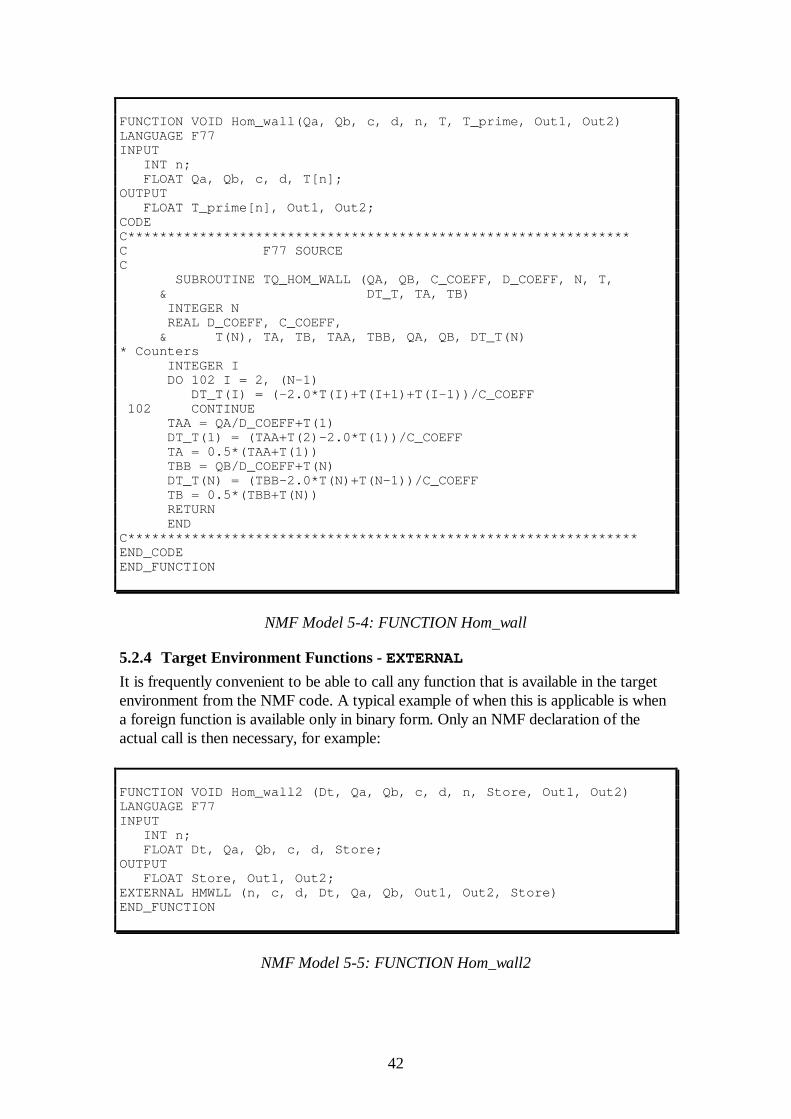
42
FUNCTION VOID Hom_wall(Qa, Qb, c, d, n, T, T_prime, Out1, Out2)LANGUAGE F77INPUT INT n; FLOAT Qa, Qb, c, d, T[n];OUTPUT FLOAT T_prime[n], Out1, Out2;CODEC***************************************************************C F77 SOURCEC SUBROUTINE TQ_HOM_WALL (QA, QB, C_COEFF, D_COEFF, N, T, & DT_T, TA, TB) INTEGER N REAL D_COEFF, C_COEFF, & T(N), TA, TB, TAA, TBB, QA, QB, DT_T(N)* Counters INTEGER I DO 102 I = 2, (N-1) DT_T(I) = (-2.0*T(I)+T(I+1)+T(I-1))/C_COEFF 102 CONTINUE TAA = QA/D_COEFF+T(1) DT_T(1) = (TAA+T(2)-2.0*T(1))/C_COEFF TA = 0.5*(TAA+T(1)) TBB = QB/D_COEFF+T(N) DT_T(N) = (TBB-2.0*T(N)+T(N-1))/C_COEFF TB = 0.5*(TBB+T(N)) RETURN ENDC****************************************************************END_CODEEND_FUNCTION
NMF Model 5-4: FUNCTION Hom_wall
5.2.4 Target Environment Functions - EXTERNAL
It is frequently convenient to be able to call any function that is available in the targetenvironment from the NMF code. A typical example of when this is applicable is whena foreign function is available only in binary form. Only an NMF declaration of theactual call is then necessary, for example:
FUNCTION VOID Hom_wall2 (Dt, Qa, Qb, c, d, n, Store, Out1, Out2)LANGUAGE F77INPUT INT n; FLOAT Dt, Qa, Qb, c, d, Store;OUTPUT FLOAT Store, Out1, Out2;EXTERNAL HMWLL (n, c, d, Dt, Qa, Qb, Out1, Out2, Store)END_FUNCTION
NMF Model 5-5: FUNCTION Hom_wall2
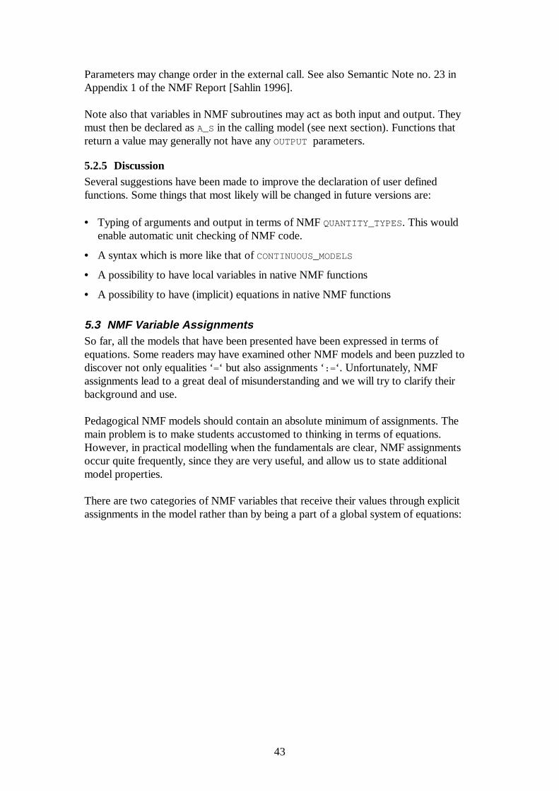
43
Parameters may change order in the external call. See also Semantic Note no. 23 inAppendix 1 of the NMF Report [Sahlin 1996].
Note also that variables in NMF subroutines may act as both input and output. Theymust then be declared as A_S in the calling model (see next section). Functions thatreturn a value may generally not have any OUTPUT parameters.
5.2.5 DiscussionSeveral suggestions have been made to improve the declaration of user definedfunctions. Some things that most likely will be changed in future versions are:
• Typing of arguments and output in terms of NMF QUANTITY_TYPES. This wouldenable automatic unit checking of NMF code.
• A syntax which is more like that of CONTINUOUS_MODELS
• A possibility to have local variables in native NMF functions
• A possibility to have (implicit) equations in native NMF functions
5.3 NMF Variable AssignmentsSo far, all the models that have been presented have been expressed in terms ofequations. Some readers may have examined other NMF models and been puzzled todiscover not only equalities ‘=‘ but also assignments ‘:= ‘. Unfortunately, NMFassignments lead to a great deal of misunderstanding and we will try to clarify theirbackground and use.
Pedagogical NMF models should contain an absolute minimum of assignments. Themain problem is to make students accustomed to thinking in terms of equations.However, in practical modelling when the fundamentals are clear, NMF assignmentsoccur quite frequently, since they are very useful, and allow us to state additionalmodel properties.
There are two categories of NMF variables that receive their values through explicitassignments in the model rather than by being a part of a global system of equations:
44
category NMF role description
Locallyassignedvariables
LOC • Locally assigned variables receive their value byassignment. Assignments to LOC variables are inmost respects equivalent to equations with a singledeclared good inverse
• Their fundamental job is to carry subroutine outputinto equation evaluation
• They may also occur in some other convenientconstructions, where equations are not allowed
• They must be assigned to before they are referred
• They may remain unassigned, but must not beassigned repeatedly
• They may not occur in links
• They may not occur as time derivatives
Assigned statevariables
A_S • Assigned variables retain their values from onetimestep to the next
• They are necessary in order to express models thatcan have multiple modes (or states), such as athermostat
• They must be referred before they are assigned to
• They must be assigned to once, never repeatedly
• They may not occur in links
• They may not occur as time derivatives
5.3.1 Locally Assigned VariablesAs we have seen, NMF allows calling of external functions and subroutines. This is animportant gateway to already existing models, which can be turned into NMF with asimple “wrapper.” It also enables coding of special algorithms that are beyond thescope of straight NMF or that are proprietary in nature and that therefore aredistributed in binary form. However, even if the actual model is hidden in a subroutine,(trivial) equations must be declared in the calling NMF model. The basic rules forcalling external subroutines are:
1. Subroutine output must be stored in a LOC or A_S variable.
2. Subroutine input may be any expression of present variables and parameters,excluding those that are assigned as output in the same call.

45
The NMF rule that there must be one explicit equation (declared “=“ sign) per OUT
variable still applies.
Let us pretend for a moment that the finite difference approximation of the wall modelfrom Section 5.1.2 is a trade secret, that we would like to contain in a binary EXTERNAL
routine. The “wrapper” model could then take the following form:
CONTINUOUS_MODEL tq_hom_wall_wrapped
ABSTRACT "A 1D finite difference wall model. One homogeneous layer. TQ interfaces on both sides."
EQUATIONS
/*Hom_wall was declared in Section 5.2.3 */
CALL Hom_wall(Qa, Qb, c_coeff, d_coeff, n, State, Temp, Out1, Out2);
/* wrapper equations */ FOR i = 1, n State'[i] = Temp[i]; END_FOR ;
0 = -Ta + Out1; 0 = -Tb + Out2;
LINKS
/* type name variables .... */
TQ a_side Ta, POS_IN Qa ; TQ b_side Tb, POS_IN Qb ;
VARIABLES
/* type name role def min max description*/
generic State[n] OUT "Internal State vector" Temp Ta IN 0. abs_zero BIG "a-side surface temp" Temp Tb IN 0. abs_zero BIG "b-side surface temp" HeatFlux Qa OUT 0. -BIG BIG "a-side entering heat" HeatFlux Qb OUT 0. -BIG BIG "b-side entering heat" generic Temp[n] LOC "Local for State " Temp Out1 LOC "Local for Out1 " Temp Out2 LOC "Local for Out2 "
MODEL_PARAMETERS
/* type name role def min max description */ INT n SMP 3 3 BIGINT "no of internal states"
PARAMETERS
/* type name role def min max description */
Area a S_P 10. SMALL BIG "wall area" Length thick S_P .25 SMALL BIG "wall total thickness" HeatCondL lambda S_P 0.5 SMALL BIG "heat transfer coeff" Density rho S_P 2000. SMALL BIG "wall density" HeatCapM cp S_P 900. SMALL BIG "wall heat capacity"

46
generic c_coeff C_P "internal coeff." generic d_coeff C_P "internal coeff." generic e_coeff C_P "internal coeff."
PARAMETER_PROCESSING
/*Hom_wall_proc was declared in Section 5.2.1 */
CALL Hom_wall_proc(a, thick, lambda, rho, cp, n, c_coeff, d_coeff, e_coeff);
END_MODEL
NMF Model 5-6: tq_hom_wall_wrapped
In the wall model, the “wrapper equations” are indeed trivial and therefore seem rathersuperfluous. Usually, the wrapper contains some meaningful conversion, for example,from one set of units to another.
Note that the IN/OUT partitioning of the link variables has been changed in this versionof the wall model. The subroutine input arguments (Cf. Section 5.2.3) Qa and Qb havebeen declared as OUT variables of the NMF model to illustrate the fact that subroutineinputs may be any expression of present NMF variables. This will lead to a ratherawkward calculation algorithm in an input/output oriented environment, including acall to a numerical equation solver. Depending on other environment characteristicsthis may or may not influence the overall calculation work in any significant way.Typically, it will have little influence on the overall execution time in a simultaneoussolver for real-scale problem sizes.
It is fundamental to understand that subroutine input may depend on model OUT
variables. However, since this leads to more complicated generated code for someenvironments, it rarely occurs in practice.
Explicit local assignment of LOC variables is equivalent to a subroutine call. Theassignment modelling repertoire that was presented in the PARAMETER_PROCESSING
section (3.7.6) may be used in the EQUATION section as well for LOC (and A_S)
variables. A typical structure is that a model is in either on or off mode:
/* Excerpt from Annex 17 chiller*/
IF Gamma <= 0 OR M_fl_c <= 0 OR M_fl_e <= 0 OR T_in_e <= T_set OR Q_reg <= 0 THEN /* The chiller is off */ T_ex_e := T_in_e ; T_evap := 0 ; Qevap := 0 ; Power := 0 ; Qcond := 0 ; Cop := 0 ; Status := 0 ; Optime := 0 ; Power_c := 0 ; H_tran_e := 0 ; H_tran_c := 0 ;
47
ELSE /* The chiller is on */ Status := IF Q_reg < q_min THEN 1 ELSE_IF Q_reg < q_max THEN 2 ELSE 3 END_IF;
Qevap := IF Q_reg < q_min THEN q_min ELSE_IF Q_reg < q_max THEN Q_reg ELSE q_max END_IF;
Optime := IF Q_reg < q_min THEN Q_reg / q_min ELSE_IF Q_reg < q_max THEN 1 ELSE 1 END_IF;
T_ex_e := T_in_e - Qevap / M_fl_e / CP_WAT ; Etaev := 1 - EXP (- auev / M_fl_e / CP_WAT) ; T_evap := T_in_e - (T_in_e - T_ex_e) / Etaev ; Etacd := 1 - EXP (- aucd / M_fl_c / CP_WAT) ; Ct := CRTemp (icompr, T_cond, T_evap) ; Pl := Qevap / q_max * Ct ; Fl := PLFACT (icompr, Pl) ;
T_diff := T_cond - T_evap; Cop := IF T_diff < -1E-4 OR T_diff > 1E-4 THEN Fl * etacar * (-ABS_ZERO + T_evap) / T_diff ELSE 1 END_IF;
Power := Qevap / Cop ; Qcond := Qevap + Power ; Power_c := Power * Optime ; H_tran_e := Qevap * Optime ; H_tran_c := Qcond * Optime ; END_IF ;
Statements enclosed by IF … THEN … ELSE … END_IF structures must in NMF beassignments. For equations, only conditional expressions are available.
The previous example, and any other conditional structure, can always be convertedinto equivalent equations. The only fundamental difference is that in assignment form, avariable may remain unassigned and without a defined value, while in equation formsome (dummy) equation must always be in effect.
From Section 3.8 we have

48
IF test <= 1 THEN a := 2 ELSE_IF test > 3 THEN a := 4END_IF;
In this case, a (a LOC variable) will not always be defined. The phrase can be convertedinto an equivalent equation for a (an IN or OUT variable):
a = IF test <= 1 THEN 2 ELSE_IF test > 3 THEN 4 ELSE 0 /* or some other arbitrary value*/ END_IF;
5.3.1.1 DiscussionThe main advantage of the use of local assignments is that the modeller may, in acompact form, give advice about an efficient solution algorithm. Such an algorithmmay be nearly impossible to deduce by automatic symbolic methods, since verycomplex condition structures may have to be successfully analyzed.
For many solvers, the cost of an additional local assignment in a model is nearlynegligible, since it will not add to the dimension of the global system matrix. Therefore,any variable that can be turned into a local assignment should. A model is consideredto be of better quality if all potential local assignments have been utilized. Examples ofvariables that could have been converted into locals in previous examples are thevirtual temperatures Taa and Tbb of the wall model in Section 5.1.2, and the localpressure drop dp in the leak model of Section 4.4.2.
A limitation of NMF v. 3.02 is that variable limits must be constants. A trick to check avariable against arbitrary limits with the introduction of an additional local variable isthe following. Assume that the variable var is to be kept between lo_expr andhi_expr .
The condition can then be written and simplified,
lo_expr < var < hi_expr,
0 < var - lo_expr < hi_expr - lo_expr,
0 < (var - lo_expr)/(hi_expr - lo_expr) < 1.
Introducing the local variable Test ,
Test := (var - lo_expr)/(hi_expr - lo_expr)
allows us to rewrite the condition with constant limits
0 < Test < 1.
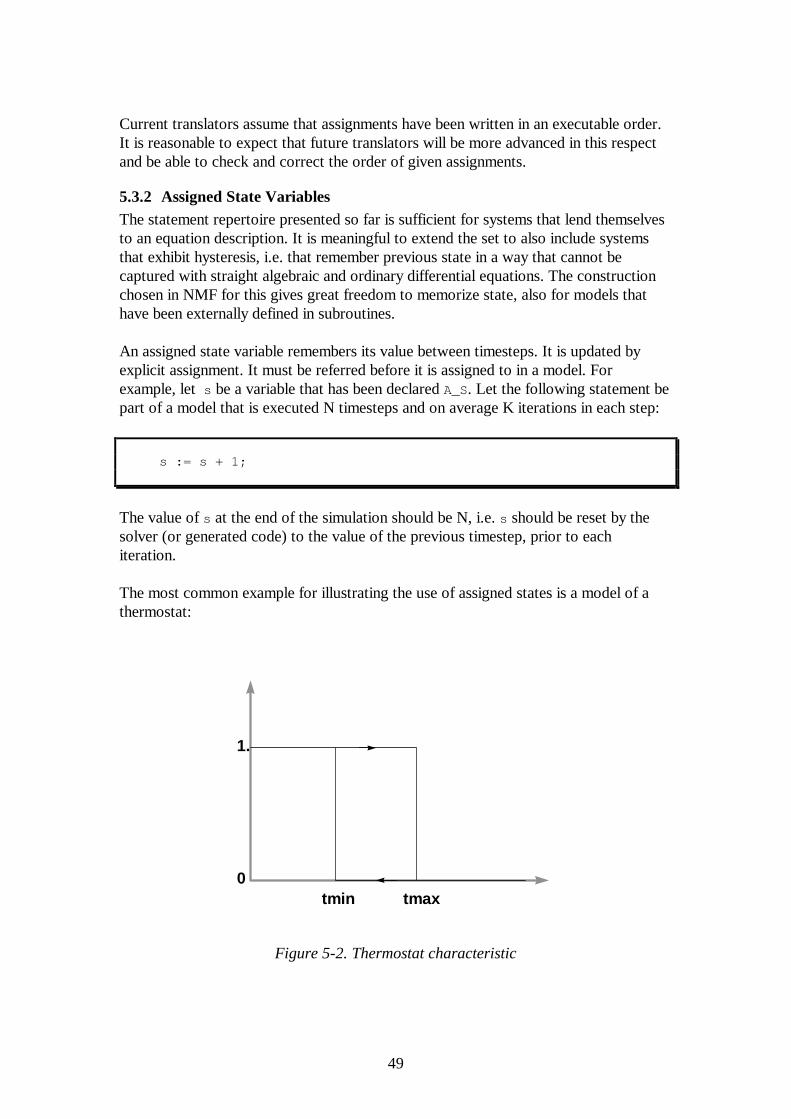
49
Current translators assume that assignments have been written in an executable order.It is reasonable to expect that future translators will be more advanced in this respectand be able to check and correct the order of given assignments.
5.3.2 Assigned State VariablesThe statement repertoire presented so far is sufficient for systems that lend themselvesto an equation description. It is meaningful to extend the set to also include systemsthat exhibit hysteresis, i.e. that remember previous state in a way that cannot becaptured with straight algebraic and ordinary differential equations. The constructionchosen in NMF for this gives great freedom to memorize state, also for models thathave been externally defined in subroutines.
An assigned state variable remembers its value between timesteps. It is updated byexplicit assignment. It must be referred before it is assigned to in a model. Forexample, let s be a variable that has been declared A_S. Let the following statement bepart of a model that is executed N timesteps and on average K iterations in each step:
s := s + 1;
The value of s at the end of the simulation should be N, i.e. s should be reset by thesolver (or generated code) to the value of the previous timestep, prior to eachiteration.
The most common example for illustrating the use of assigned states is a model of athermostat:
tmin tmax0
1.
Figure 5-2. Thermostat characteristic
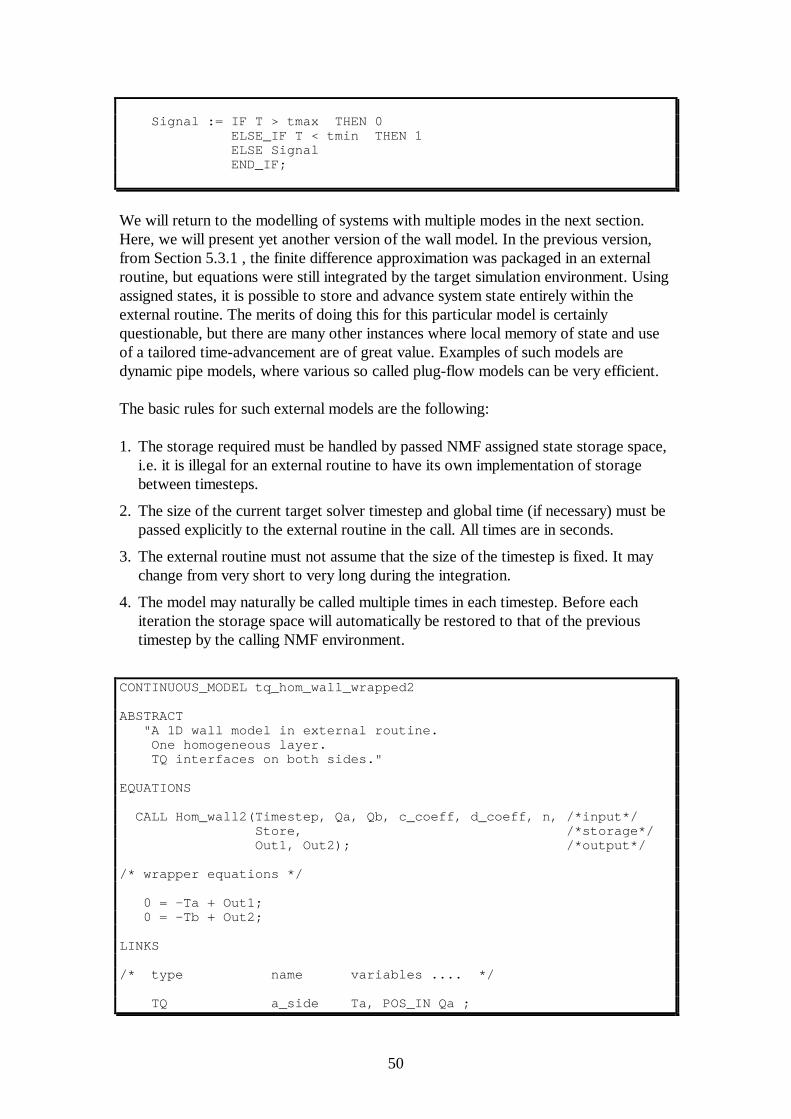
50
Signal := IF T > tmax THEN 0 ELSE_IF T < tmin THEN 1 ELSE Signal END_IF;
We will return to the modelling of systems with multiple modes in the next section.Here, we will present yet another version of the wall model. In the previous version,from Section 5.3.1 , the finite difference approximation was packaged in an externalroutine, but equations were still integrated by the target simulation environment. Usingassigned states, it is possible to store and advance system state entirely within theexternal routine. The merits of doing this for this particular model is certainlyquestionable, but there are many other instances where local memory of state and useof a tailored time-advancement are of great value. Examples of such models aredynamic pipe models, where various so called plug-flow models can be very efficient.
The basic rules for such external models are the following:
1. The storage required must be handled by passed NMF assigned state storage space,i.e. it is illegal for an external routine to have its own implementation of storagebetween timesteps.
2. The size of the current target solver timestep and global time (if necessary) must bepassed explicitly to the external routine in the call. All times are in seconds.
3. The external routine must not assume that the size of the timestep is fixed. It maychange from very short to very long during the integration.
4. The model may naturally be called multiple times in each timestep. Before eachiteration the storage space will automatically be restored to that of the previoustimestep by the calling NMF environment.
CONTINUOUS_MODEL tq_hom_wall_wrapped2
ABSTRACT "A 1D wall model in external routine. One homogeneous layer. TQ interfaces on both sides."
EQUATIONS
CALL Hom_wall2(Timestep, Qa, Qb, c_coeff, d_coeff, n, /*input*/ Store, /*storage*/ Out1, Out2); /*output*/
/* wrapper equations */
0 = -Ta + Out1; 0 = -Tb + Out2;
LINKS
/* type name variables .... */
TQ a_side Ta, POS_IN Qa ;
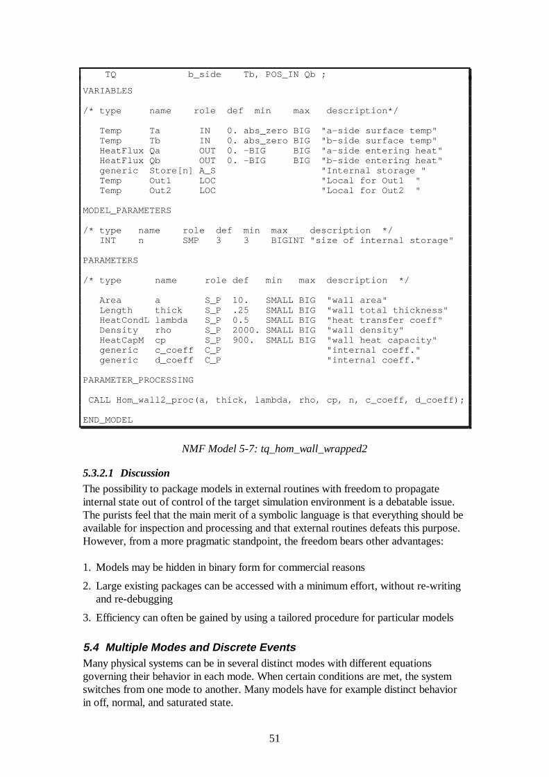
51
TQ b_side Tb, POS_IN Qb ;
VARIABLES
/* type name role def min max description*/
Temp Ta IN 0. abs_zero BIG "a-side surface temp" Temp Tb IN 0. abs_zero BIG "b-side surface temp" HeatFlux Qa OUT 0. -BIG BIG "a-side entering heat" HeatFlux Qb OUT 0. -BIG BIG "b-side entering heat" generic Store[n] A_S "Internal storage " Temp Out1 LOC "Local for Out1 " Temp Out2 LOC "Local for Out2 "
MODEL_PARAMETERS
/* type name role def min max description */ INT n SMP 3 3 BIGINT "size of internal storage"
PARAMETERS
/* type name role def min max description */
Area a S_P 10. SMALL BIG "wall area" Length thick S_P .25 SMALL BIG "wall total thickness" HeatCondL lambda S_P 0.5 SMALL BIG "heat transfer coeff" Density rho S_P 2000. SMALL BIG "wall density" HeatCapM cp S_P 900. SMALL BIG "wall heat capacity" generic c_coeff C_P "internal coeff." generic d_coeff C_P "internal coeff."
PARAMETER_PROCESSING
CALL Hom_wall2_proc(a, thick, lambda, rho, cp, n, c_coeff, d_coeff);
END_MODEL
NMF Model 5-7: tq_hom_wall_wrapped2
5.3.2.1 DiscussionThe possibility to package models in external routines with freedom to propagateinternal state out of control of the target simulation environment is a debatable issue.The purists feel that the main merit of a symbolic language is that everything should beavailable for inspection and processing and that external routines defeats this purpose.However, from a more pragmatic standpoint, the freedom bears other advantages:
1. Models may be hidden in binary form for commercial reasons
2. Large existing packages can be accessed with a minimum effort, without re-writingand re-debugging
3. Efficiency can often be gained by using a tailored procedure for particular models
5.4 Multiple Modes and Discrete EventsMany physical systems can be in several distinct modes with different equationsgoverning their behavior in each mode. When certain conditions are met, the systemswitches from one mode to another. Many models have for example distinct behaviorin off, normal, and saturated state.
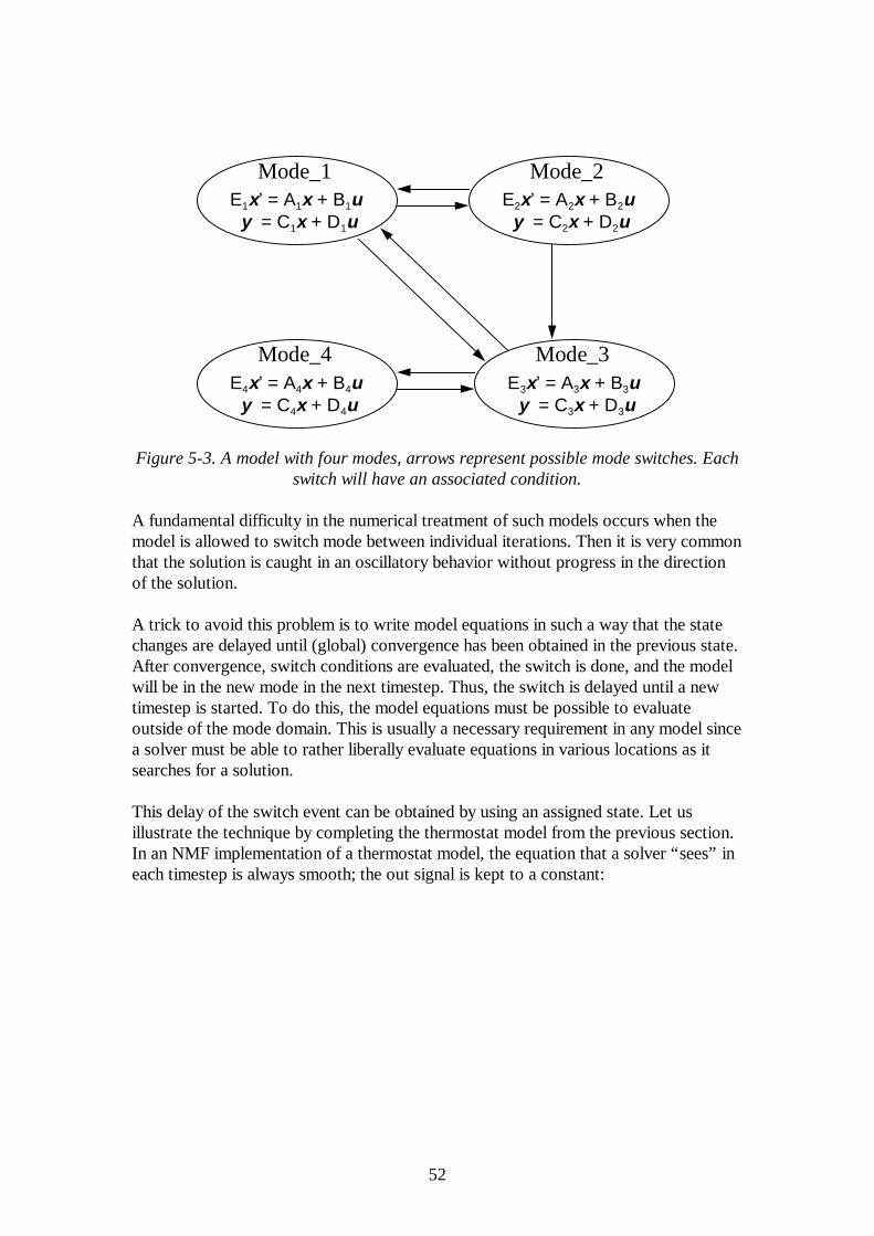
52
E1x’ = A1x + B1u y = C1x + D1u
Mode_1
E3x’ = A3x + B3u y = C3x + D3u
Mode_3E4x’ = A4x + B4u y = C4x + D4u
Mode_4
E2x’ = A2x + B2u y = C2x + D2u
Mode_2
Figure 5-3. A model with four modes, arrows represent possible mode switches. Eachswitch will have an associated condition.
A fundamental difficulty in the numerical treatment of such models occurs when themodel is allowed to switch mode between individual iterations. Then it is very commonthat the solution is caught in an oscillatory behavior without progress in the directionof the solution.
A trick to avoid this problem is to write model equations in such a way that the statechanges are delayed until (global) convergence has been obtained in the previous state.After convergence, switch conditions are evaluated, the switch is done, and the modelwill be in the new mode in the next timestep. Thus, the switch is delayed until a newtimestep is started. To do this, the model equations must be possible to evaluateoutside of the mode domain. This is usually a necessary requirement in any model sincea solver must be able to rather liberally evaluate equations in various locations as itsearches for a solution.
This delay of the switch event can be obtained by using an assigned state. Let usillustrate the technique by completing the thermostat model from the previous section.In an NMF implementation of a thermostat model, the equation that a solver “sees” ineach timestep is always smooth; the out signal is kept to a constant:

53
CONTINUOUS_MODEL Thermostat_no_events
ABSTRACT "Thermostat w dead band tmin-tmax, OFF=0, ON=1 at low temperature. No event calls."
EQUATIONS
Out_signal = Old_signal; /* Old_signal will be maintained constant in each timestep*/
/* since Old_signal is an A_S, it should be assigned to after being referred to*/
Old_signal := IF T > tmax THEN 0 ELSE_IF T < tmin THEN 1 ELSE Old_signal END_IF ;
LINKS
/* type name variables */
ControlLink Out_sign Out_signal ; ControlLink In_sign T ;
VARIABLES
/* type name role def min max description */
generic Old_signal A_S "State On or Off" generic T IN "In-signal" generic Out_signal OUT 0 0 1 "Out-signal On=1 or Off=0"
PARAMETERS
/* type name role def min max description */
temp tmin S_P "lower limit of dead band " temp tmax S_P "higher limit of dead band"
END_MODEL
NMF Model 5-8: Thermostat_no_events
This model will always overshoot the switch event by some fraction of the currenttimestep. Thus if nothing else is done, there will be a time step dependent error, whichmay become large in, e.g., a variable timestep environment. A remedy for this problemis presented in Section 5.4.2.
Hysteresis can occur in unexpected places, and is not always associated with physicalfriction. Regard for example the bdleak model among the Multizone Air Exchangemodels. A physical leak with finite volume will “remember its state” by the properties(temperature) of the air in the leak cavity.
54
5.4.1 A General Framework for Multimode ModelsNMF does not allow separate equations for each mode. A single set of equations mustbe valid at all times, and conditions must be contained in these. Thus multimodeequations should be written in the following general form:
0 = IF Mode == 1 THEN <expression 1> ELSE_IF Mode == 2 THEN <expression 2> ELSE_IF Mode == 3 THEN <expression 3> ELSE <expression 4> END_IF
The update of the assigned state Mode is done after the actual equations have beendeclared. The set of switches in Figure 5-3 can, e.g., be implemented in the followingway:
IF <1->2 expression> >= 0 AND Mode == 1 THEN Mode :=2 END_IF;IF <1->3 expression> >= 0 AND Mode == 1 THEN Mode :=3 END_IF;IF <2->3 expression> >= 0 AND Mode == 2 THEN Mode :=3 END_IF;IF <2->1 expression> >= 0 AND Mode == 2 THEN Mode :=1 END_IF;IF <3->1 expression> >= 0 AND Mode == 3 THEN Mode :=1 END_IF;IF <3->4 expression> >= 0 AND Mode == 3 THEN Mode :=4 END_IF;IF <4->3 expression> >= 0 AND Mode == 4 THEN Mode :=3 END_IF;
where the expressions are assumed to be formulated in such a way that zero iscrossed from negative to positive when the switch shall occur. This construction allowsinsertion of arbitrary algorithmic code at switches. We will motivate the chosenconstruction further in the next section, where we turn our attention to the signaling ofdiscrete events to a solver.
5.4.2 Signaling Discrete EventsThe method presented for multimode modelling may lead to an overshoot of the event,since the switch is delayed until the end of the current timestep. This is a problem witha variable timestep solver, which, if everything else is behaving smoothly, may takevery long steps.
For this reason, many solvers are able to detect event signals from the model. Whensuch a signal has been detected, the solver can go into an event-location mode, andwith more or less sophisticated methods, determine the precise location of the switchand finish the timestep just before. After a short step across the discontinuity, normaltime stepping is resumed.
Three NMF functions are dedicated to event signaling, EVENT, EVENTN, and EVENTP.They take two arguments, an assigned state variable and a signal (an expression), thezero crossing of which signifies an event. EVENTP flags an event only when the signal
55
goes from negative to positive, EVENTN from positive to negative, and EVENT in anydirection. The event functions will compare the present value of the signal with the (inthe A_S) memorized past value, signal the event if necessary, update the A_S variable,and return the current signal value.
It is important to make sure that the event functions are actually updated as necessary,and not lie buried in some logical structure. Hence the proposed event switchingconstruction in the general framework, where all event functions are updated in everyiteration. Tailored constructions are obviously applicable in individual cases.
IF Eventp(G[1], <1->2 expr> ) >= 0 AND Mode == 1 THEN Mode :=2 END_IF;IF Eventp(G[2], <1->3 expr> ) >= 0 AND Mode == 1 THEN Mode :=3 END_IF;IF Eventp(G[3], <2->3 expr> ) >= 0 AND Mode == 2 THEN Mode :=3 END_IF;IF Eventp(G[4], <2->1 expr> ) >= 0 AND Mode == 2 THEN Mode :=1 END_IF;IF Eventp(G[5], <3->1 expr> ) >= 0 AND Mode == 3 THEN Mode :=1 END_IF;IF Eventp(G[6], <3->4 expr> ) >= 0 AND Mode == 3 THEN Mode :=4 END_IF;IF Eventp(G[7], <4->3 expr> ) >= 0 AND Mode == 4 THEN Mode :=3 END_IF;
Both Mode and G must be declared as A_S variables.
5.4.2.1 DiscussionThe requirement of an explicitly declared memory variable in the event functions maybe perceived as unnecessary. Surely this variable could be introduced automatically bya translator. This is true, and “auto-expandable” versions of the event functions couldeasily be furnished with future NMF versions. However, the main motivation for thepresent construction is that event calls may also occur in external code. The same istrue for the chosen method of modelling hysteresis, and for any other NMF systemroutine, as LINEARIZE or NMF_ERROR. NMF’s ability to accommodate sophisticatedexternal models is an important feature which is often lost when typical models indifferent formalisms are compared and discussed.
The final version of the thermostat model with event calls can be examined inAppendix 2 of the NMF report. Notice the explicit calls to event functions to ensurethat they are always evaluated. The event functions are special in that they have an I/Oargument (the A_S). In general, functions are allowed to return only a single value.
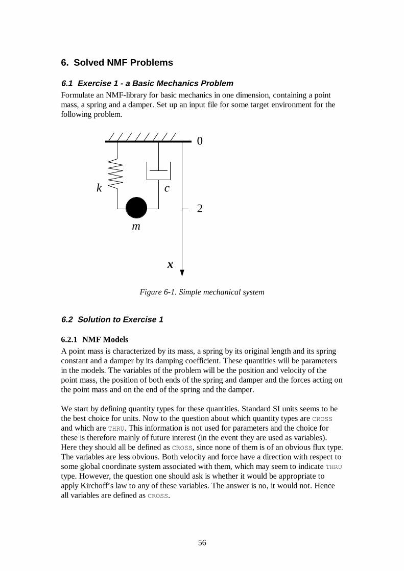
56
6. Solved NMF Problems
6.1 Exercise 1 - a Basic Mechanics ProblemFormulate an NMF-library for basic mechanics in one dimension, containing a pointmass, a spring and a damper. Set up an input file for some target environment for thefollowing problem.
x
0
2
m
ck
Figure 6-1. Simple mechanical system
6.2 Solution to Exercise 1
6.2.1 NMF ModelsA point mass is characterized by its mass, a spring by its original length and its springconstant and a damper by its damping coefficient. These quantities will be parametersin the models. The variables of the problem will be the position and velocity of thepoint mass, the position of both ends of the spring and damper and the forces acting onthe point mass and on the end of the spring and the damper.
We start by defining quantity types for these quantities. Standard SI units seems to bethe best choice for units. Now to the question about which quantity types are CROSS
and which are THRU. This information is not used for parameters and the choice forthese is therefore mainly of future interest (in the event they are used as variables).Here they should all be defined as CROSS, since none of them is of an obvious flux type.The variables are less obvious. Both velocity and force have a direction with respect tosome global coordinate system associated with them, which may seem to indicate THRU
type. However, the question one should ask is whether it would be appropriate toapply Kirchoff’s law to any of these variables. The answer is no, it would not. Henceall variables are defined as CROSS.
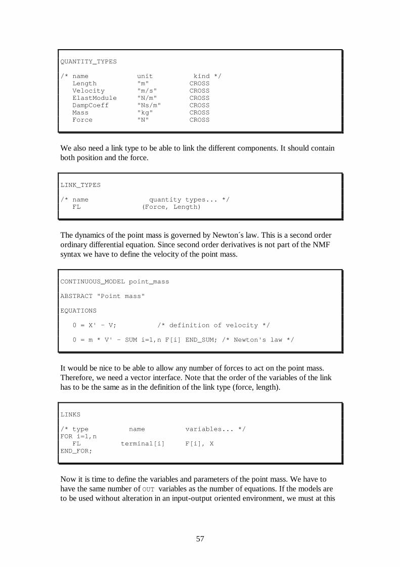
57
QUANTITY_TYPES
/* name unit kind */ Length "m" CROSS Velocity "m/s" CROSS ElastModule "N/m" CROSS DampCoeff "Ns/m" CROSS Mass "kg" CROSS Force "N" CROSS
We also need a link type to be able to link the different components. It should containboth position and the force.
LINK_TYPES
/* name quantity types... */ FL (Force, Length)
The dynamics of the point mass is governed by Newton´s law. This is a second orderordinary differential equation. Since second order derivatives is not part of the NMFsyntax we have to define the velocity of the point mass.
CONTINUOUS_MODEL point_mass
ABSTRACT "Point mass"
EQUATIONS
0 = X' - V; /* definition of velocity */
0 = m * V' - SUM i=1,n F[i] END_SUM; /* Newton's law */
It would be nice to be able to allow any number of forces to act on the point mass.Therefore, we need a vector interface. Note that the order of the variables of the linkhas to be the same as in the definition of the link type (force, length).
LINKS
/* type name variables... */FOR i=1,n FL terminal[i] F[i], XEND_FOR;
Now it is time to define the variables and parameters of the point mass. We have tohave the same number of OUT variables as the number of equations. If the models areto be used without alteration in an input-output oriented environment, we must at this
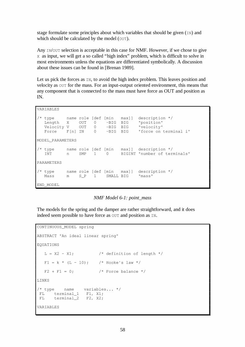
58
stage formulate some principles about which variables that should be given (IN ) andwhich should be calculated by the model (OUT).
Any IN /OUT selection is acceptable in this case for NMF. However, if we chose to giveX as input, we will get a so called “high index” problem, which is difficult to solve inmost environments unless the equations are differentiated symbolically. A discussionabout these issues can be found in [Brenan 1989].
Let us pick the forces as IN , to avoid the high index problem. This leaves position andvelocity as OUT for the mass. For an input-output oriented environment, this means thatany component that is connected to the mass must have force as OUT and position asIN.
VARIABLES
/* type name role [def [min max]] description */ Length X OUT 0 -BIG BIG "position" Velocity V OUT 0 -BIG BIG "velocity" Force F[n] IN 0 -BIG BIG "force on terminal i"
MODEL_PARAMETERS
/* type name role [def [min max]] description */ INT n SMP 1 0 BIGINT "number of terminals"
PARAMETERS
/* type name role [def [min max]] description */ Mass m S_P 1 SMALL BIG "mass"
END_MODEL
NMF Model 6-1: point_mass
The models for the spring and the damper are rather straightforward, and it doesindeed seem possible to have force as OUT and position as IN .
CONTINUOUS_MODEL spring
ABSTRACT "An ideal linear spring"
EQUATIONS
L = X2 - X1; /* definition of length */
F1 = k * (L - l0); /* Hooke's law */
F2 + F1 = 0; /* Force balance */
LINKS
/* type name variables... */ FL terminal_1 F1, X1; FL terminal_2 F2, X2;
VARIABLES
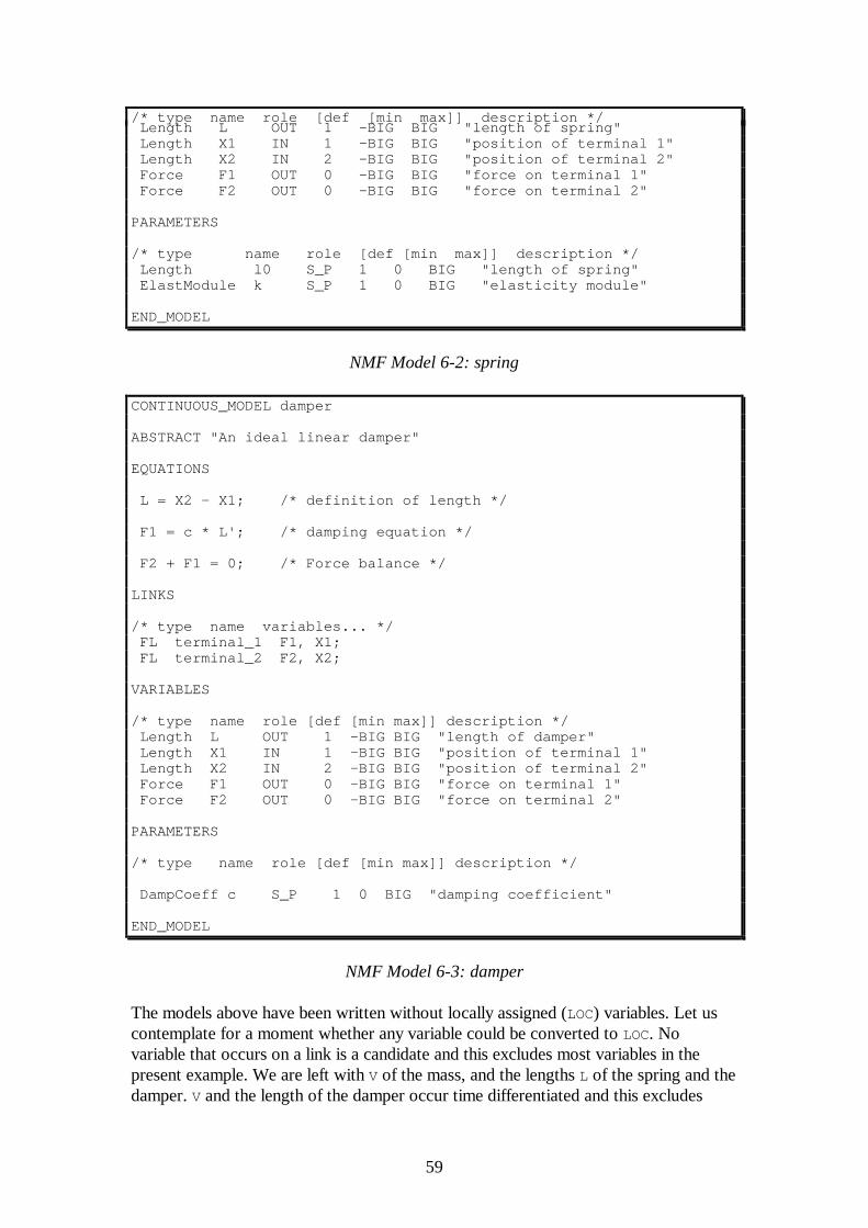
59
/* type name role [def [min max]] description */ Length L OUT 1 -BIG BIG "length of spring" Length X1 IN 1 -BIG BIG "position of terminal 1" Length X2 IN 2 -BIG BIG "position of terminal 2" Force F1 OUT 0 -BIG BIG "force on terminal 1" Force F2 OUT 0 -BIG BIG "force on terminal 2"
PARAMETERS
/* type name role [def [min max]] description */ Length l0 S_P 1 0 BIG "length of spring" ElastModule k S_P 1 0 BIG "elasticity module"
END_MODEL
NMF Model 6-2: spring
CONTINUOUS_MODEL damper
ABSTRACT "An ideal linear damper"
EQUATIONS
L = X2 - X1; /* definition of length */
F1 = c * L'; /* damping equation */
F2 + F1 = 0; /* Force balance */
LINKS
/* type name variables... */ FL terminal_1 F1, X1; FL terminal_2 F2, X2;
VARIABLES
/* type name role [def [min max]] description */ Length L OUT 1 -BIG BIG "length of damper" Length X1 IN 1 -BIG BIG "position of terminal 1" Length X2 IN 2 -BIG BIG "position of terminal 2" Force F1 OUT 0 -BIG BIG "force on terminal 1" Force F2 OUT 0 -BIG BIG "force on terminal 2"
PARAMETERS
/* type name role [def [min max]] description */
DampCoeff c S_P 1 0 BIG "damping coefficient"
END_MODEL
NMF Model 6-3: damper
The models above have been written without locally assigned (LOC) variables. Let uscontemplate for a moment whether any variable could be converted to LOC. Novariable that occurs on a link is a candidate and this excludes most variables in thepresent example. We are left with V of the mass, and the lengths L of the spring and thedamper. V and the length of the damper occur time differentiated and this excludes
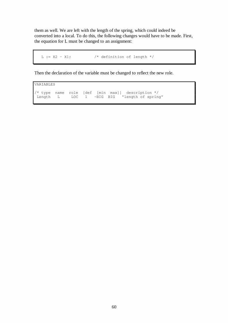
60
them as well. We are left with the length of the spring, which could indeed beconverted into a local. To do this, the following changes would have to be made. First,the equation for L must be changed to an assignment:
L := X2 - X1; /* definition of length */
Then the declaration of the variable must be changed to reflect the new role.
VARIABLES
/* type name role [def [min max]] description */ Length L LOC 1 -BIG BIG "length of spring"
61
6.2.2 Input file for IDA SolverBelow is an input file for IDA Solver for the system configuration of Exercise 1. TheIN /OUT partitioning of the variables in the NMF models have, as previously discussed,been selected to avoid IN -IN and OUT-OUT connections for the given configuration.However, in an input-output free environment like IDA Solver any connection ispermitted, and springs and dampers can for example be connected in series.
Some comments have been added to clarify meanings of file statements.
ABSTRACT"Simple test of exercise 1mechancis library"
!logical and physical filesFILES OUTPUT OUTPUT1 PATH MECH.PRNEND_FILES
! declare model instances! P - point mass! S - spring! D - damperMODULES MODULE P TYPE Point_mass! parameters for Pn 2m 1
MODULE S TYPE Springk 1l0 1
MODULE D TYPE Damperc 1END_MODULES
!Connect the instances. Variable!level connections are used in!this exampleCONNECTIONS P.F(1) = S.F2 P.F(2) = D.F2 P.X = S.X2 P.X = D.X2END_CONNECTIONS
!Define boundary valuesBOUNDARIESS.X1 0D.X1 0END_BOUNDARIES
!Define initial valuesSTART_VALUESDEFAULT 0P.X 2P.V 0D.X2 2D.L 2S.X2 2S.L 2END_START_VALUES
!Specify integration dataINTEGRATION FROM 0. TO 10.!Initial time step to be used STEP 0.0001!Overall error tolerance TOL 0.001!Switch limit between relative!and absolute tolerance TOL_LIM 1.
!Specify output data LIST OUT_ALL OUT_TIMES 0 1 1 END_TIMES
P.X Position S.F1 Spring_force D.F1 Damper_force END
LOG FILE OUTPUT1 P.X Position S.F1 Spring_force D.F1 Damper_force ENDEND_INTEGRATION
62
7. References
Andersson, M., 1990, An Object-Oriented Language for Model Representation,Licentiate Thesis, Dept. of Automatic Control, LIT , Box 118, 221 00 Lund, Sweden,May 1990, CODEN:LUTFD2/(TFRT-3208)/1-102/(1990)
Bonneau, D., F.X. Rongere, D. Covalet, B. Gautier, 1993, CLIM 2000 - ModularSoftware for Energy Simulation in Buildings, Conference proc. BuildingSimulation'93, IBPSA, Adelaide, Australia, Aug. 1993
Brenan, K.E., S.L. Campbell, and L.R. Petzold, 1989, Numerical Solution ofInitial-Value Problems in Differential-Algebraic Equations, North Holland
Bring, A., P. Sahlin, 1993, Modelling Air Flows and Buildings with NMF and IDA,Conference proc. Building Simulation'93, IBPSA, Adelaide, Australia, Aug. 1993
Bring, A., L. Eriksson, H. Hermansson, M. Lindgren, P. Sahlin, 1995, IDA - anEnvironment for Building and Energy Systems Simulation, Conference proc. BuildingSimulation'95, IBPSA, Madison, WI, USA, Aug. 1995
Buhl, W.F., E. Erdem, F.C. Winkelmann, E.F. Sowell, 1993, Recent Improvementsin SPARK: Strong Component Decomposition, Multivalued Objects, and GraphicalInterface, Conference proc. Building Simulation'93, IBPSA, Adelaide, Australia, Aug.1993
Clark, D.R., 1985, HVACSIM+ Building Systems and Equipment SimulationProgram - Reference Manual, National Institute of Standards and Technology,Washington D.C.
Clarke, J.A., D.F. Mac Randall, 1993, The Energy Kernel System: Form andContent, Conference proc. Building Simulation'93, IBPSA, Adelaide, Australia, Aug.1993
Dubois, A.M., 1988, MODEL-BASED COMPUTER AIDED MODELLING: the newperspectives for building energy simulation, communication from CSTB, B.P. 21,06561 VALBONNE Cedex, France
Elmquist, H., 1978, A Structured Model Language for Large Continuous Systems,Phd thesis, Lund Institute of Technology
Elmqvist, H., 1986, LICS: Language for Implementation of Control Systems, Dept.of Automatic Control, LIT , Box 118, 221 00 Lund, Sweden
Grozman, P., P. Sahlin, 1996, ASHRAE RP-839 NMF Translator - User’s Guide,ASHRAE Inc. and Bris Data AB
63
ISO TC 184, 1993, The STEP Standard, draft international standard DIS 10303,continuously since 1992 published in several different parts
Jeandel, A., F. Favret, E. Lariviere, 1993, ALLAN.Simulation - a General SoftwareTool for Model Description and Simulation, Conference proc. Building Simulation'93,IBPSA, Adelaide, Australia, Aug. 1993
Kolsaker, K., 1994a, NEUTRAN-supported NMF Enhancements, presented to the TC4.7 NMF Ad Hoc Subcommittee at the ASHRAE winter meeting 1994
Kolsaker, K., 1994b, Simpler NMF Description of Advanced Models UsingHierarchical Modelling and Data Abstraction, presented to the TC 4.7 NMF Ad HocSubcommittee at the ASHRAE annual meeting 1994
Kolsaker, K., 1994c, NEUTRAN - A Translator of Models from NMF into IDA andSPARK, Proceeding to the BEPAC conference, BEP'94, York
Lorenz, F., 1987, Reflections about Representation Methods, proc. workshop on thefuture of building energy modelling, Ispra, Italy, Nov. 1987, CEC EUR 11603 ENPREPRINT, May 1988
Lorenz, F., 1990, Brief Description of the MS1 (Modelling System 1) Project, privatecommunication
Lorenz, F., 1994, Comments on the Neutral model Format, presented to the TC 4.7NMF Ad Hoc Subcommittee at the ASHRAE winter meeting 1994
Nataf J.-M. 1994, Translator from NMF to SPARK, Conference proc. BuildingSimulation'95, IBPSA, Madison, WI, USA, Aug. 1995
Ohlsson, B., A. Persson, 1991, Sandys - a simulation program for electrical circuitsand systems, ABB Review 5/91
Pelletret, R., 1994a, Personal communication
Pelletret, R., S. Soubra, 1994b, Standardizing Model Documentation - ThePROFORMA Experience, presented to the TC 4.7 NMF Ad Hoc Subcommittee at theASHRAE winter meeting 1994
Pelletret, R., S. Soubra, W. Kielholz, 1995, Transferring Simulation Techniques toEnd-Users - Application to TRNSYS, Conference proc. Building Simulation'95,IBPSA, Madison, WI, USA, Aug. 1995
Sahlin, P., A.Bring, 1993, Applying IDA to Airflow Problems in Buildings, ITMreport 1993:3
Sahlin, P., A. Bring, 1995, The IDA Multizone Air Exchange Application, Bris DataAB and Div. of Building Services Engineering, KTH
64
Sahlin P., A. Bring, K. Kolsaker, 1995, Future Trends of the Neutral Model Format,Conference proc. Building Simulation'95, IBPSA, Madison, WI, USA, Aug. 1995
Sahlin, P., A.Bring, E.F.Sowell, 1996, The Neutral Model Format for BuildingSimulation, Version 3.02, Report, Dept. of Building Sciences, KTH, Stockholm(available at ftp://urd.ce.kth.se/pub/reports/nmfre302.rtf)
Sahlin, P., C. Johansson, 1994, NMF-Based Aspect Models in STEP for Buildingand Process Plant Simulation, proc. of the CIC W78 workshop on computerintegrated construction, Aug. 22-24, 1994, VTT, Helsinki, Finland
Sahlin, P, E.F. Sowell, 1989, A Neutral Format for Building Simulation Models,proc. of Building Simulation ´89 , Vancouver, BC, International Building PerformanceSimulation Association
Shapovalov, A., 1995, personal communication
Yi Jiang , Zhenxi Xu, Feng Chen, 1994, TUHVAC - an object oriented computersoftware for HVAC design, analysis and simulation, preprints of the 4th Intnl. Conf.on System Simulation in Buildings, Dec, 1994, Liege, Belgium
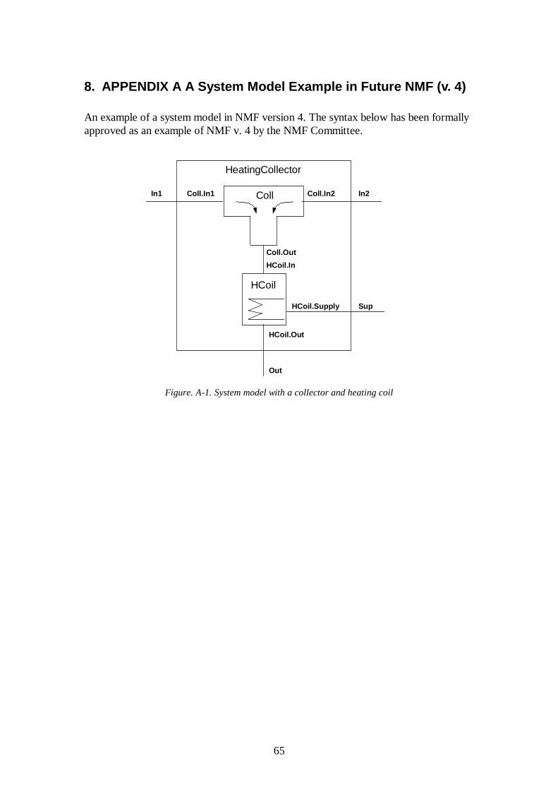
65
8. APPENDIX A A System Model Example in Future NMF (v. 4)
An example of a system model in NMF version 4. The syntax below has been formallyapproved as an example of NMF v. 4 by the NMF Committee.
Coll
HCoil
HeatingCollector
Out
HCoil.Out
HCoil.In
Coll.Out
Coll.In1 Coll.In2In1 In2
HCoil.Supply Sup
Figure. A-1. System model with a collector and heating coil
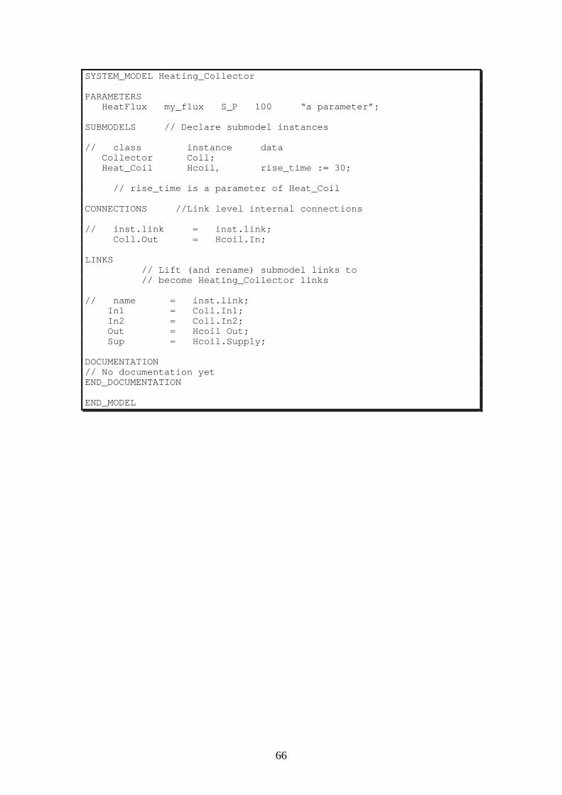
66
SYSTEM_MODEL Heating_Collector
PARAMETERS HeatFlux my_flux S_P 100 “a parameter”;
SUBMODELS // Declare submodel instances
// class instance data Collector Coll; Heat_Coil Hcoil, rise_time := 30;
// rise_time is a parameter of Heat_Coil
CONNECTIONS //Link level internal connections
// inst.link = inst.link; Coll.Out = Hcoil.In;
LINKS // Lift (and rename) submodel links to // become Heating_Collector links
// name = inst.link; In1 = Coll.In1; In2 = Coll.In2; Out = Hcoil Out; Sup = Hcoil.Supply;
DOCUMENTATION// No documentation yetEND_DOCUMENTATION
END_MODEL