New Jersey Geological and Water SurveyGeological Survey Report GSR 42

BOREHOLE GEOPHYSICAL LOGS AND GEOLOGICAL INTERPRETATION

OF TWO DEEP, OPEN BOREHOLES IN THE PASSAIC FORMATION,

ELIZABETH CITY, UNION COUNTY, NEW JERSEY

N.J. Department of Environmental Protection - Water Resources Management

STATE OF NEW JERSEYChris Christie, GovernorKim Guadagno, Lieutenant Governor

Department of Environmental ProtectionBob Martin, Commissioner

Water Resources ManagementDaniel Kennedy, Assistant Commissioner

Geological and Water SurveyKarl Muessig, State Geologist

NEW JERSEY DEPARTMENT OF ENVIRONMENTAL PROTECTION

The mission of the New Jersey Department of Environmental Protection is to assist the residents of New Jersey in preserving, sustaining, protecting and enhancing the environment to ensure the integration of high environmental quality, public health and economic vitality.

NEW JERSEY GEOLOGICAL AND WATER SURVEY

The mission of the New Jersey Geological and Water Survey (NJGWS) is to map, research, interpret and provide scientific information regard ing the state’s geology and groundwater resources. This information supports the regulatory and planning functions of DEP and other governmental agencies and provides the business community and public with information necessary to address environmental concerns and make economic decisions.

Geological Survey Reports (ISSN 0741-7357) are published by the New Jersey Geological and Water Survey, P.O. Box 420, Mail stop 29-01, Trenton, NJ 08625-0420. This report may be reproduced in whole or part provided that suitable reference to the source of the copied material is provided.

More information on NJGWS reports and the price list is available on the Survey’s website: www.njgeology.org.

Use of brand, commercial, or trade names is for identification purposes only and does not constitute endorsement by the New Jersey Geological and Water Survey.

For more information, contact: ` New Jersey Department of Environmental Protection Division of Water Supply and Geoscience New Jersey Geological and Water Survey P.O. Box 420, Mail Code 29-01Trenton, NJ 08625-0420(609) 292-1185http://www.njgeology.org/

Cover illustration: Geophysical logging at the ETES geothermal well field in April 2012. Mark French is pictured overseeing activities.

New Jersey Geological and Water Survey

Geological Survey Report GSR 42

Borehole Geophysical Logs and Geological Interpretation of Two Deep, Open Boreholes in the Passaic Formation,

Elizabeth City, Union County, NJ

by

Gregory C. Herman, Mark A. French, and John F. CurranNew Jersey Geological and Water Survey

New Jersey Department of Environmental ProtectionWater Resources Management

New Jersey Geological and Water SurveyP.O. Box 420, Mail Code 29-01

Trenton, NJ 08625-04202015

CONTENTS

Introduction ..................................................................................................................................................................1Geological Setting .......................................................................................................................................................2Well Parameters and Geophysical Logs .......................................................................................................................2Stratigraphy .................................................................................................................................................................4Borehole Telemetry and Structural Geology ...............................................................................................................8Borehole Model Using Google EarthTM (GE) .............................................................................................................12Hydrogeology .............................................................................................................................................................14Geothermal Gradient and Fluid-Temperature Anomalies ...........................................................................................15Nature of the Deep Water-Bearing Zone and the Crustal In-Situ Stress Regime .......................................................17Discussion ...................................................................................................................................................................20Acknowledgements .....................................................................................................................................................20References ...................................................................................................................................................................21

FIGURES

1. Approximate location of ETES geothermal boreholes EG1 and EG20 that were logged by the NJGWS ...........12. Generalized geologic map and profile geometry of the covered stratigraphic section ..........................................33. The penetrated section relative to Newark Basin formations and aquifers .............................................................44. Geophysical logs and borehole diagrams ..............................................................................................................55. Examples of red mudstone and gray shale from EG20 ...........................................................................................66. Examples of red mudstone and gray shale from EG1 .............................................................................................67. Borehole sections showing local alteration of the rock ..........................................................................................78. Structural-feature orientation analyses of BTV data for boreholes EG1 and EG20 ...............................................99. EG1 structural-feature orientation analyses of OBTV data and scatterplot of fracture dip versus fracture quantity .....................................................................................................................................................1010. Scatterplot of fracture aperture versus depth ....................................................................................................... 1111. Examples of late-stage extension veins cutting sub-horizontal veins with apparent offset .................................1212. Map view of a virtual well-field model in Google Eart TM (GE) of deep-bedrock well EG1 and EG20 ............1313. An oblique view looking west through the GE model .........................................................................................1414. Profile and map diagrams detailing methods used to construct the GE mode ....................................................1515. NNE view of the GE model showing details of the deep water-bearing zone .....................................................1616. Generalized geologic map of the New York recess (A) centered on the Newark Basin comparing early Mesozoic tectonic elements with the in-situ crustal stress regime .............................................................1717. Schematic diagrams illustrating an elliptical borehole profile (A) related to the in-situ crustal stres regime, local extension fractures, and light artifacts in a OBI record .................................................................1818. Sections of the EG1 OBI record showing light artifacts centered on 140o and 320o trends ................................19

TABLES

1. Identification, location, and GE-model parameters for boreholes EG1 and EG2 .................................................22. Primary and secondary structural planes measured in OBTV records of EG1 and EG20 .....................................103. The depth, range, number, and estimated vertical thickness of gently-dipping gypsum veins interpreted from the OBI records of EG1 and EG20................................................................................................................11

CONTENTS (continued)

APPENDICES

1. Support information about the NJ Geological and Water Survey borehole televiewer and heat-pulse flow-meter instruments and method .....................................................................................................................232. NJGWS structural planes and borehole telemetry parameters for the EG1 and EG20 OBI-40 records ...............27

Digital-data file download using a compressed-file format (GSR42.zip) containing the following files:

NJGWS GSR42 Borehole EG1_1773_UP360c.pdf (3.69 MB) - Adobe Systems Incorporated©, Adobe Portable Document File (PDF) of interpreted OBI-40 record of borehole EG1 NJGWS GSR42 Borehole EG20_1426_UP360c.pdf (1.98 MB) - Adobe Systems Incorporated©, Adobe Portable Dcoument File (PDF) of interpreted OBI-40 record of borehole EG20 NJGWS GSR42 - Elizabeth Geothermal.kmz (123 KB) - Google Inc.©, Google Earth Keyhole Markup

Language (KMZ) 3D model with OBI-40 structural interpretations of boreholes EG1 and EG20 including geophysical logs. NJGWS GSR42 Appendix 2.xlsx - Microsoft Excel® (2010) workbook containing worksheets for borehole EG1 and EG20, including depth, telemetery, and structural-feature parameters measured in the OBI-40 records

Earth Tech Energy Solutions (ETES) informed the NJ Geological and Water Survey (NJGWS) in July 2011 that deep bedrock boreholes were planned as part of a geothermal heat pump system installation in downtown Elizabeth City, Union County, N.J. (fig. 1). Approxi-mately 20 boreholes of about 7-3/4 to 10-inch diameter would be drilled to depths of as much as 2000 feet (ft) or about 610 meters (m) below land surface (bls). The wells would be open to bedrock below the cased depths, start-ing at about 275 ft (~84 m) bls. The NJGWS is currently compiling geothermal information as part of a national effort to promote renewable energy sources (Herman and others, 2012), therefore, the Survey expressed an in-terest in contributing to the study as it offered an oppor-tunity to characterize geo-thermal properties and the structural framework of a bedrock aquifer in an urban environment having very limited surface exposures.

By April 2012, more than 20 deep boreholes had been drilled in a ½-acre parking lot located northeast and adjacent to a commercial building complex for which the system was designed (fig.1C and D). NJGWS was given access to log two of these boreholes from April 25th to April 30th, 2012. Geophysical logs were collected to a maxi-mum depth of about 1776 ft (541 m) bls. These in-cluded continuous records of the fluid temperature, fluid electrical resistivity/conductivity, caliper (well diameter), natural gamma ray radioactivity, forma-tion single-point electri-cal resistance, electrical self-potential and an opti-

BOREHOLE GEOPHYSICAL LOGS AND GEOLOGICAL INTERPRETATION OF TWO DEEP, OPEN BOREHOLES IN THE PASSAIC FORMATION,

ELIZABETH CITY, UNION COUNTY, NJ

INTRODUCTION

Figure 1. Approximate location of ETES geothermal boreholes EG1 and EG20 that were logged by the NJGWS.

cal borehole image (OBI) of the borehole wall. Spot measurements of borehole flow were also taken in each hole using a heat-pulse flow meter (HPFM – see Ap-pendix 1). The logs were processed, interpreted, and archived soon afterward. This report summarizes the study results including: 1) an interpretation of sub-surface geological structures from photographed and measured stratigraphic bed planes and non-bedding fractures; 2) water-bearing (permeable) features; 3) formation and borehole-fluid geophysical logs; and 4) a three-dimensional (3D) computer model thatwas designed for interactive display and examination of the subsurface geology using Google Earth ™.

GEOLOGICAL SETTING

The site is located near the intersection of Jefferson Avenue and East Jersey Street in downtown Elizabeth City, N.J, within the Elizabeth, N.J., 7-1/2 minute top-ographic quadrangle (fig. 1). The site also sits on the southeast edge of the NJ part of the Newark Basin (fig.2). Outcrop exposure is poor due to the urban develop-ment and most of the existing geological information in the area is compiled from previous subsurface borings and wells. Less than 50 ft of unconsolidated sedimen-tary cover overlies Triassic age red and gray mudstone and shale of the Passaic Formation (Stanford, 1995). Bedrock dips about 13o northwest (Drake and others, 1996). Figure 2A shows a map view of the penetrat-

is commonly stopped upon passing into casing while logging upward. Galvanized steel casing develops a magnetic dipole that locally perturbs Earth’s local mag-netic field which distorts the record close to the bottom of the casing. BTV interpretations are therefore useful on the open borehole sections whereas other geophysi-cal logs, like natural gamma radiation and fluid tem-perature are typically run through casing. An unstable power source used during OBTV logging required two logging runs in each hole that overlapped, with upper and lower record segments that required joining dur-ing subsequent data processing. Appendix 1 includes schematic illustrations of the OBTV (OBI-40 by the manufacturer) and HPFM tools, and a brief explanation of logging specifications and methods of deployment.

The geophysical records were processed and inter-preted in May, 2012. The natural gamma and caliper logs were combined with the OBI images using WellCAD v.4.4 computer software (figs. 5-7). WellCAD® image

WELL PARAMETERS AND GEOPHYSICAL LOGS

Table 1 lists the identification, location and construc-tion characteristics of boreholes EG1 and EG20. ETES drilled each borehole with an air-rotary rig using 10- and 7-inch-diameter drill bits. The larger bit was used for installing temporary, 10-inch-diameter steel casing from land surface to 280 ft (85 m) in EG1 and to 275 ft (84 m) in EG20. However, the temporary casing in EG20 was pulled and replaced by a short length (~11 ft) of casing prior to logging. The casing was used to help stabilize and guide drilling to greater depths when using the smaller-diameter bit. Each borehole now con-tains a closed geothermal loop consisting of a small-di-ameter feed and return lines that are cemented in place.

Geophysical logs collected in each borehole (fig.4) include borehole diameter (caliper), natural gamma,fluid temperature and electrical conductivity/resistiv-ity, formation single-point electrical resistance, forma-tion self-potential, optical borehole televiewer (OBTV), and a heat-pulse flow meter (HPFM). OBTV recording

2

ed section of the lower part of the Passaic Formation with respect to gray-bed marker units identified here as being part of the Ukrainian, Kilmer, Neshanic, and Perkasie Members of Olsen and others (1996). These marker beds are taken from work by Drake and others (1996) and were extrapolated from the central part of the basin beyond the terminal moraine where outcrops are more common than in the Elizabeth area. Figure 2B illustrates the method used to estimate the profilethickness of the penetrated section and figure 3 shows the approximate stratigraphic interval covered in this study with respect to strata and aquifers of the New-ark Basin (Herman and others, 1998; Herman, 2010).

Identification

Geographic coordinates(WGS84 - decimal degrees) Elevation NGVD88 – feet (meters)

NJ Permit Land

StickupCasing Borehole

Name Number Longitude Latitude surface depth depth

GEModel

Altitude

EG1 2700016708 -74.213062 40.66573326

(7.9)1.5

(0.5)10*

(3.0)1774 (540.9)

1804(550)

EG20 2700016708 -74.212704 40.66552228

(8.5)2.0

(0.6)280

(85.4)1427 (435.0)

1806(550.6)

Table 1. Identification, location, and GE-model parameters for boreholes EG1 and EG20

*EG1 had ~275 feet (84 meters) of 10-inch-diameter casing installed at one time, but it was pulled and replacedwith about 11 feet of 10-inch casing prior to logging.

Figure 2. Generalized geologic map and profile geometry of the covered stratigraphic section

3

Martinsville

Weston

Somerset

Rutgers

Ukranian Mbr

New Brunswick South Amboy Keyport

RARITANBAY

Roselle

Kilmer M

br

Nesh

anic M

br

Perkasie M

br

Elizabeth

NJ

NY

penetrate

d sect

ion

WISCO

NSIN

AN

Passaic Flood Tunnel borings

and cores

Jersey City

EXPLANATIONLate Triassic to Early Jurassic sedimentary and igneous rocks of the Newark Basin

Diabase

Lockatong Formation

Basalt

Passaic Formation

Stockton Formation

Feltville, Towaco, andBoonton Formations

Passaic Formation gray and black beds

Lockatong Formation red beds

ConglomerateNewark Basin CoringProject corehole

63 0 3 6 Kilometers

10000 0 10000 20000 30000 Feet

Boreholes EG1 and

EG20 penetrated

section

Compositedistribution of dark gray andblack bedsbeneath thePreaknessBasaltadapted from Olsen andothers (1996)

Hook Mt. Basalt

Orange Mt. Basalt

Top of the UkranianMember of the

Passaic Formation

Base of the Kilmer Member of the

Passaic Formation

Top of the T-U Member of the

Passaic Formation

Base of the Q Member of the

Passaic Formation

Top of the Neshanic Member of the

Passaic Formation

diabase

and deviation modules were used to conduct a structural analysis of the visible primary and secondary geo-logical planes. Primary planes are contacts between mudstone and silt-stone beds whereas secondary planes are fractures other than those lying along stratigraphic contacts. Fractures lacking any visible accumulations of secondary minerals infilling frac-ture interstices are classified simply as fractures whereas the mineralized fractures are noted as veins. Appendix 2 includes a Microsoft Excel® work-book summarizing the sets of struc-tural measurements for each borehole including alphabetic variables describ-ing the structural features, and numeric ones denoting structural depths, plane dip, plane dip direction (DipAzm), the borehole tilt (BHTilt), and tilt direction (BHAzm) for each interpreted plane. These variables were used for subse-quent structural trend analyses and to generate 3D computer models of the boreholes and interpreted structures.

The wells were not thoroughly de-veloped prior to OBTV logging. Con-sequently, each well contains sections where natural cross flows were weak and the borehole water was muddy and turbid, resulting in sections with poor borehole imagery and no geologi-cal interpretation. In sections having stronger cross flows, the water was clearer, the OBTV image quality was fair to good, bedding and fractures are visible in the borehole wall, and structural interpretation was possible. Figure 4 graphically combines the log results of both wells and summarizes the interpreted and obscure sections for each hole. Geo-logical sections were obtained in EG1 from about 274 ft to 1428 ft (84 m to 435 m) bls, and in EG20 from about 11 ft to 290 ft (3m to 88 m) bls (fig. 6). How-ever, structural measurements were only obtained in EG20 to about 275 ft (84 m) because of turbidity and a

4

Figure 3. The penetrated section relative to Newark Basin formations and aquifers.

borehole-diameter change below 280 ft (85 m). The in-terpreted section of each borehole nearly overlaps, and combines in having a near-continuous geological sec-tion for the site from about 11 ft to 1428 ft (3 m to 435 m) bls (fig. 6). The integrated and interpreted logs are printed and output at a depth scale of 1 inch = 20 ft

STRATIGRAPHY

The bulk of the stratigraphic section consists of dif-ferent types of brownish-red mudstone simply referred to here as ‘red’ mudstone (figs. 5-7). Thin sections of

laminated shale are interpreted as gray-shale beds (or simply ‘gray beds’) that are optically masked by red muddy water. Many different types of red mudstones oc-

TURB

ID

TURB

ID

Figure 4. Geophysical logs and borehole diagrams.

cur within the Newark Basin (Smoot and Olsen, 1985; 1994). These are commonly referred to as ‘massive’, the term being used in a broad sense, for rocks that tend to have a blocky or hackly appearance in a weathered out-crop and that show little obvious internal structure on su-perficial examination (Smoot and Olsen, 1985). In con-trast, an OBTV record provides a continuous, subsurface scan of a rock section not subject to surface-weathering and thus captures the stratigraphic sequence with clar-ity where the borehole water is clear. Root-disrupted (fig. 5A), vesicular (fig. 6A), and ‘featureless’ (fig. 6C) types of mudstones are the most abundant in this sec-tion, whereas mud-cracked, burrowed, and sand-patch types are more scarce. However, it is likely that the fine, telltale features of mudstone identified in outcrop

and core as desiccated or bioturbated, are in many in-stances beyond the OBTV image resolution.

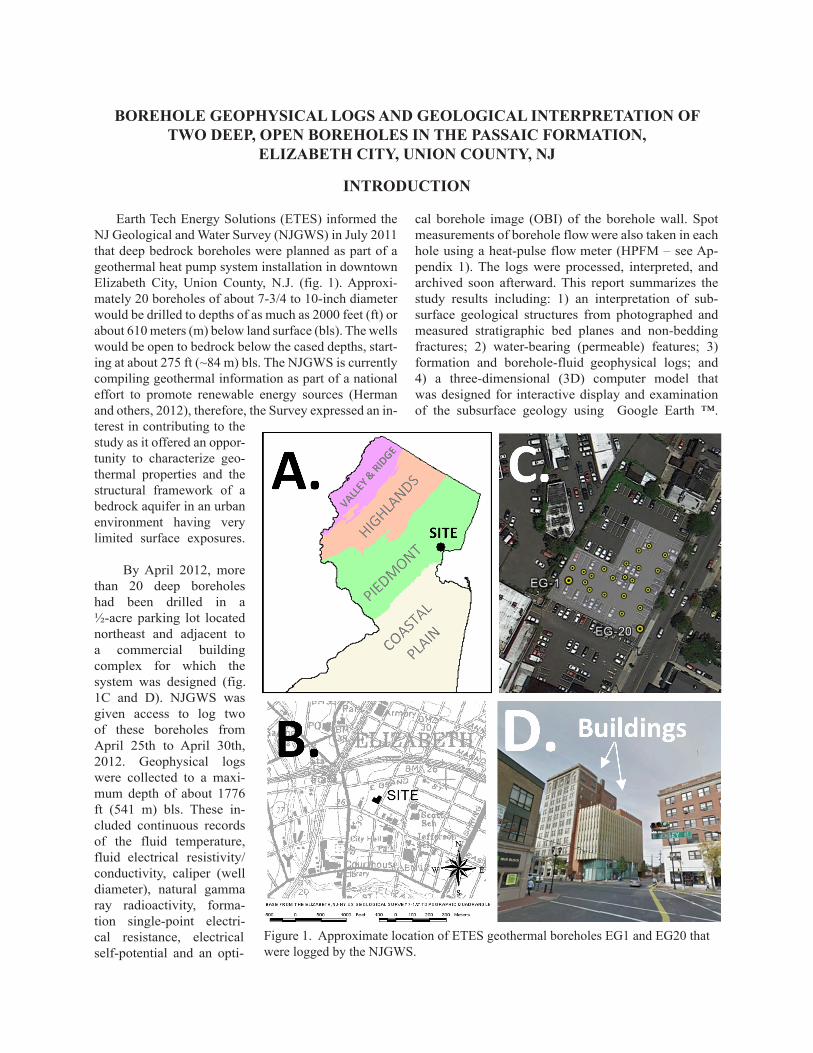
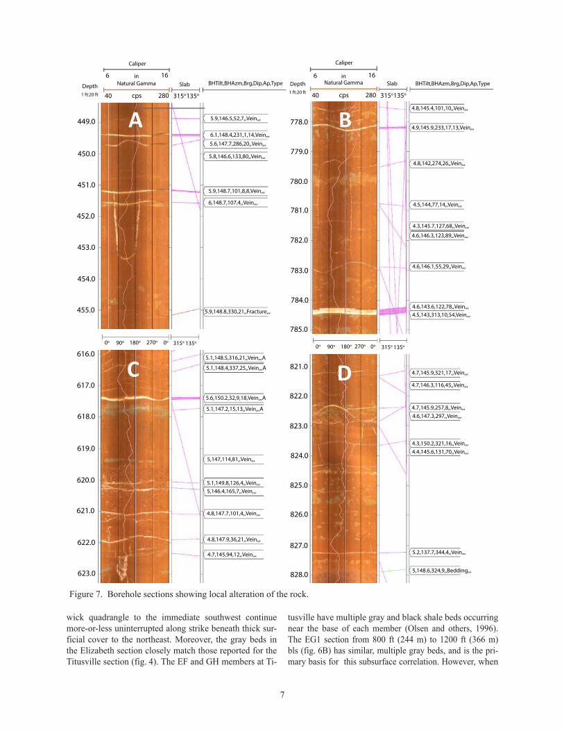
The OBTV imagery also shows that many sections of red mudstone are locally altered and mottled with light-greenish gray ovoid blebs, or light-greenish-gray tabular patches aligned along bedding planes (fig. 7) or bracketing thin, planar accumulations of white to light-gray, secondary minerals that infill interstices of gently- to-steeply-dipping secondary fractures (figs. 5B, 6A, and 6C). The ovoid blebs range in size from a few millimeters (mm) to tens of mm in diameter and occur in sections containing root-disrupted mudstone. These features probably stem from iron reduction, or iron re-moval from root growth and plant uptake prior to burial

5

A

B

C

Figure 5. Examples of red mudstone and gray shale from EG20.

A

B

C Figure 6. Examples of red mudstone and gray shale from EG1.

and compaction, because the long axes of many blebs are oriented parallel to the bedding plane (fig.7), thereby reflecting subsequent sedimentary loading and compac-tion. Similar features are reported by Smoot and Olsen (1988) as ‘reduction halos’ associated with calcite-filled, tubular root casts. Otherwise, reduction halos in mineralized bedding and fracture planes have not been widely stud-ied and recorded in the Newark Basin. However, this type of ma-trix alteration has been observed in some secondary, calcite-filledfractures in a rock core taken from the middle part of the Pas-saic Formation in Hopewell, New Jersey (Herman, 2001). Parnell and Monson (1995) point out that reduction of metal ions occurs in basin rocks subjected to low-Eh (organic-rich) environments with calcite veining and the migration of hydrocarbons and sulfides at vari-ous places and times in the basin. The composite section formed by boreholes EG1 and EG20 contains about eight sets of gray shale beds that are rhythmically distributed throughout the sec-tion otherwise dominated by red beds (for example, fig. 5B and 6B). These ‘gray’ marker beds graphically depict Late Triassic cyclic sedimentation noted by Van Houten (1965) and Olsen and others (1996). Most of these beds are only 1 or 2 ft (< 1 m) thick, but some are as much as 11 ft (3 m) thick (fig. 4). This pen-etrated section covers most of the lower part of the Passaic Forma-tion and the lower gray zone of the Brunswick aquifer (Herman and others, 2010) based on both surface and subsurface consid-erations (figs. 2 and 3). Figure 2 shows the map expression of the penetrated section within and below the Perkasie Member, as-suming that gray marker beds that crop out in the New Bruns-

6

A

B

C

D

5.9,146.5,52,7,,Vein,,,

6.1,148.4,231,1,14,Vein,,,5.6,147.7,286,20,,Vein,,,

5.8,146.6,133,80,,Vein,,,

5.9,148.7,101,8,8,Vein,,,

6,148.7,107,4,,Vein,,,

5.9,148.8,330,21,,Fracture,,,

5.1,148.5,316,21,,Vein,,,A

5.1,148.4,337,25,,Vein,,,A

5.6,150.2,32,9,18,Vein,,,A

5.1,147.2,15,13,,Vein,,,A

5,147,114,81,,Vein,,,

5.1,149.8,126,4,,Vein,,,5,146.4,165,7,,Vein,,,

4.8,147.7,101,4,,Vein,,,

4.8,147.9,36,21,,Vein,,,

4.7,145,94,12,,Vein,,,

4.8,145.4,101,10,,Vein,,,

4.9,145.9,233,17,13,Vein,,,

4.8,142,274,26,,Vein,,,

4.5,144,77,14,,Vein,,,

4.3,145.7,127,68,,Vein,,,

4.6,146.3,123,89,,Vein,,,

4.6,146.1,55,29,,Vein,,,

4.6,143.6,122,78,,Vein,,,4.5,143,313,10,54,Vein,,,

4.7,145.9,321,17,,Vein,,,

4.7,146.3,116,45,,Vein,,,

4.7,145.9,257,8,,Vein,,,4.6,147.3,297,,Vein,,,

4.3,150.2,321,16,,Vein,,,4.4,145.6,131,70,,Vein,,,

5.2,137.7,344,4,,Vein,,,

5,148.6,324,9,,Bedding,,,

449.0

450.0

451.0

452.0

453.0

454.0

455.0

616.0

617.0

618.0

619.0

620.0

621.0

622.0

623.0

778.0

779.0

780.0

781.0

782.0

783.0

784.0

785.0

821.0

822.0

823.0

824.0

825.0

826.0

827.0

828.0

0o 90o 180o 270o 0o 315o 135o

0o 90o 180o 270o 0o 315o 135o

Depth1 ft:20 ft

Caliper

Natural Gamma

40 cps 280 135o315o

Slab BHTilt,BHAzm,Brg,Dip,Ap,Type Depth1 ft:20 ft

Caliper

16in16in6 6Natural Gamma Slab BHTilt,BHAzm,Brg,Dip,Ap,Type

40 cps 280 135o315o

Caliper

7

wick quadrangle to the immediate southwest continue more-or-less uninterrupted along strike beneath thick sur-ficial cover to the northeast. Moreover, the gray beds in the Elizabeth section closely match those reported for the Titusville section (fig. 4). The EF and GH members at Ti-

tusville have multiple gray and black shale beds occurring near the base of each member (Olsen and others, 1996). The EG1 section from 800 ft (244 m) to 1200 ft (366 m) bls (fig. 6B) has similar, multiple gray beds, and is the pri-mary basis for this subsurface correlation. However, when

Figure 7. Borehole sections showing local alteration of the rock.

8

BOREHOLE TELEMETRY AND STRUCTURAL GEOLOGY

WellCAD® provides program-output options for sav-ing OBTV structural measurements as delimited ASCII®

files, including feature depth, feature description, plane dip (0-90o) and dip direction (dip azimuth, 0-359o). The sets of structural readings from each borehole in appendix 2 were sorted, parsed and saved to new text files. These were used as input for computer software used to statisti-cally analyze plane orientations with circular histograms and lower-hemisphere, equal-angle, stereographic-pro-jection diagrams (Holcombe, 2004). One circular histo-gram and two stereonets were generated for each set of beds and fractures (fig. 8). Circular histograms utilize 10o

bins for determining dip-azimuth frequencies. The stere-onet plots are used to measure the orientations of the most common planes in a data set using density contours of plane poles and for displaying a cyclographic plot of all the measured planes (fig. 8). Table 2 lists the average bed orientation and the three most common fracture planes measured in each borehole based on pole contouring.

The structural analyses show that sedimentary bed-ding in both holes consistently dips NW 10o to 11o to-ward 323o with little variation (figure 8; EG1 - 324o and EG20 - 322o). Fracture orientations are more complex and were further analyzed with respect to the borehole telemetry parameters using Microsoft Excel® software to generate scatterplots of depth versus: 1) borehole tilt (BH Tilt), 2) borehole tilt azimuth (BH-Azimuth), 3) fea-ture dip azimuth, and 4) feature (fig. 9). The borehole tilt plot for EG1 shows a sharp break from lower to higher tilts after the driller changed from using a 10-inch drill bit above ~280 ft bls to a 7-inch one below (fig. 9A). Variation in borehole azimuth is less scattered below this same depth (fig. 9B) and settles into a consistent trend with an average bearing of 144o that closely op-poses the dip direction of bedding (average 323o). This means the borehole curves gently down section in the general direction opposing bed dip. The graph of fea-ture-dip azimuth (fig. 9C) shows that most structures cluster in two preferred directions, one varying about bedding dip, and the other in the opposite direction vary-ing around ~120o. The graph of feature dip (fig. 9D) is sectioned in 30o increments to help evaluate the verti-cal distribution of gently–dipping (<30o), moderately-dipping (30o - 59o), and steeply-dipping (>60o) structural features. This graph shows that gently-dipping features (<30o) are proportionately more abundant above 1100 ft (335 m) bls whereas steeply-dipping features (60o -89o)

are the most abundant fracture set below this depth.

More than 70 percent of the fractures measured in EG1 dip less than 20o (fig. 9E) and are filled with sec-ondary, highly reflective minerals, and lie sub-parallel to stratigraphic bedding (fig. 8). The most common gently dipping fractures in EG20 strike about 38o counterclock-wise from those in EG1, and dip in opposite directions (fig. 8, and table 2). The OBTV records show that in many places these gently-dipping veins parallel bed con-tacts, but cut them at acute angles elsewhere. The drill cuttings for all of the boreholes contained fragments of gypsum spar, suggesting that many, if not most of the gently-dipping mineralized fractures are gypsum veins that thicken the section through sub-vertical extension. Although the resolution of the OBTV imagery is insuf-ficient to positively identify all of these features as gyp-sum veins, the thickest ones seen in the OBTV records have central suture lines similar to the morphology of the late-stage gypsum veins reported from the Newark Basin Coring Project (NBCP) rock cores (El Tabakh and oth-ers, 1998; Simonson and others, 2010). However, some of the gently-dipping veins display a branching and anas-tomosing configuration that may stem from reverse shear fracturing that would also structurally thicken the section.

An estimate of the vertical elongation strain (ev) in the penetrated section stemming from sub-horizontal vein growth was calculated in order to more precisely account for its compacted thickness. This is important when com-paring stratigraphic thickness variations at different loca-tions in the basin, as for example between this section and the correlative one from the NBCP Titusville core (Olsen and others, 1996). For this calculation, we assume that the cumulate thickness of veins dipping less than 20o is wholly attributed to sub-vertical elongation from gyp-sum-vein growth. Owing to the OBTV image resolution, interpretations here only include measurements of those fracture interstices generally exceeding widths of 0.15- inch (4 mm). Therefore, an interstice thickness of 0.125 inch (2 mm) was used in the calculation for each vein with unspecified thickness (table 3). The orientations of 647 gently-dipping veins were measured in the two holes with 376 having unmeasured interstices and 171 having measured ones (appendix 2). Figure 10 charts the width, or aperture, of the measured veins that range between 0.15 and 3.0 inches (4 and 76 mm). Gently-dipping veins in EG1 were measured at depths ranging from 278 to

comparing thicknesses of the two sections, the Titus-ville section is about 50 percent thicker than the section at Elizabeth (1600 ft or 488 m at Titusville compared to

1040 ft or 317 m at Elizabeth) and is therefore a substan-tially thicker sedimentary section and is consistent with its location closer to the depositional center of the basin.

Figure 8. Structural-feature orientation analyses of BTV data for boreholes EG1 and EG20. The circular histograms (left) show dip-azimuth frequency in 10o bins, and the lower-hemisphere, equal-angle stereographic plots include contoured poles-to-planes (middle), and plane cyclographs (right). The statistics for the contour plots include calculated girdles of the most common plane orientation(s).

9

Table 2. Primary and secondary structural planes measured in OBTV records of EG and EG20.

Hole Beds (dip/dip azimuth) Fractures (dip/dip azimuth)

No. Readings Average No. Readings Plane1 Plane 2 Plane 3

EG1 50 11/324 804 23/130 29/313 77/309

EG20 17 10/322 60 6/168 42/152 8/310

Table 2. Primary and secondary structural planes measured in OBTV records of EG1 and EG20.

EG1 - Fracture dip vs. number of fractures

nni

numb

nnu

Figure 9.

A

B

C

D

E

num

ber o

f fra

ctur

es

fracture dip

Figure 9. (A - D) Structural-feature orientation analyses of OBTV data and (E) scatterplot of fracture dip versus fracture quantity for EG1.

10

Dep

th (f

eet)

Aperture (inches)

Figure 10. Scatterplot of fracture aperture versus depth.

11

1079 ft (85 to 329 m) bls, over an 800-foot (244-m) in-terval. Gently-dipping veins in EG20 were measured at depths ranging from 26 to 270 ft (8 to 82 m) bls (appen-dix 2), with most occurring between 70 to 270 ft (21 to 82 m), or about a 200-ft (6-m) interval. An estimate of total sub-horizontal vein thickness and the resulting ver-tical elongation stemming from vein growth over a total ~1000-ft (305 m) section (table 3) is 133 inches (~11 ft or 3389 mm). Therefore, the vertical elongation strain (ev) = L1 (1000 ft) – L0 (989 ft) / L0 * 100 = 1.1 %.

Moderately-to-steeply-dipping fractures are distrib-uted unevenly through the section (fig. 9D). Moderate-ly-dipping fractures are the least abundant but appear to cluster in groups that are spaced at about 100- to 200-ft (~30 to 60 m) intervals. The steeply dipping fractures are similarly grouped in sets spaced about 200 ft (61 m) apart, and there is a tendency for fracture dips to steepen downward within a cluster (fig. 9D). The deepest frac-ture group occurs between ~1300 to 1400 ft (397 to 427 m) bls and constitutes the deep water-bearing zone (figs.4 and 6C). The most common, steeply-dipping fracture sets dip 77o northwest toward azimuth 309o (77/309). This fracture set shows an apparent cross-cutting rela-tionship with the sub-horizontal (gypsum?) veins (fig.11). A subordinate, steeply-dipping set strikes parallel to the former set but dips steeply southeast (about 77/129 degrees). The latter set was estimated from the cyclo-graphic plot of all fractures in EG1 (fig. 8A). The ori-entation of fracture sets measured here with respect to those measured elsewhere in the basin is discussed later. The width of fracture interstices or fracture ‘aperture’ (fig. 10) generally increases downward from land surface to a maximum approaching 4 inches (0.33 ft or ~10 cm) at 500 ft (152 m) bls, then returns to a linear base trend of about 1 inch (25 mm) in the rest of the section. The stere-

Hole

Borehole section

containing gently

inclined veins (feet)

Total number

of gently

dipping veins

Total number having

unmeasured interstices

< 4mm

Total thickness (mm) for

unmeasured interstices assuming

2mm per vein

Total number having

measured interstices

> 4mm

Total thickness (mm) for

measured interstices

ranging from 5 to

80 mm

Total vertical

thickness (mm)

EG1 278 - 1079 572 712 116 2542 3254

EG20 26 – 270 75 20 40 55 95 135

Totals 1045 647 376 752 171 3254 3389

Table 3. Number of gently-dipping gypsum veins and estimated total vertical thickness based on the OBI interpretations.

S1

S1

gypsum vein

gypsum (?) veins

5,139.5,303,70,,Vein,,,

5.2,138.8,123,10,,Vein,,,

4.9,139.9,164,9,,Vein,,,

4.7,140,285,22,8,Vein,,,

5,145.5,122,15,,Vein,,,

5.2,145.1,358,7,,Vein,,,

5.3,142.3,310,74,,Vein,,,4.9,144.2,83,5,,Vein,,,

5.2,143.3,267,23,7,Vein,,,

5.4,143.3,182,4,8,Vein,,,

5.5,138.9,116,27,,Vein,,,

5.6,139.7,163.4,,Vein,,,

5.5,140.3,305,78,,Vein,,,

5.6,142.7,102,16,11,Vein,,,

5.5,140.1,311,36,12,Vein,,,

5.5,140.1,311,36,16,Vein,,,A

5.3,142.4,298,89,,Vein,,,

5.3,143.2,312,12,,Vein,,,

5.3,142.6,310,80,,Vein,,,

5.3,142.6,289,2,10,Vein,,,

5.2,142.2,356,2,,Vein,,,

5.1,142.7,316,23,,Vein,,,A5.1,142.4,320,3,,Vein,,,A5.1,142.4,124,15,,Vein,,,A

1024.0

1025.0

1026.0

1027.0

1028.0

1029.0

1030.0

1031.0

1032.0

1049.0

1050.0

1051.0

1052.0

1053.0

1054.0

1055.0

1056.0

1057.0

0o 90o 180o 270o 0o 315o 135o

Figure 11. Examples of late-stage extension veins cutting sub-horizontal veins with apparent offset.

BOREHOLE MODEL USING GOOGLE EARTHTM (GE)

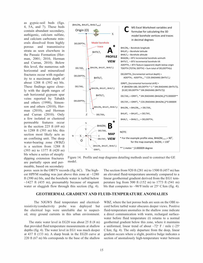
The OBTV records for both boreholes and select geophysical logs for EG1 were used to generate a 3D computer model of the interpreted subsurface geology for display in Google Earth (GE). EG20 provided a clear view of the shallow section whereas EG1 provided one of the deep section, except for the turbid interval be-tween 1427 to 1647 ft (435 to 502 m) bls (Fig. 4). GE provides a free, interactive computerized platform for dynamically viewing the distribution of the interpreted geological features with respect to borehole and geo-physical logs (Herman, 2013). Because GE only dis-plays physical features at and above Earth’s surface, the borehole model was built to project above ground (figs.12 and 13). This requires offsetting the vertical com-ponent of the model origin above its surface location by an amount exceeding the borehole depth. Therefore, rather than using the elevation of land surface for the model origin, the model origin is offset directly above its actual location by about 1778 ft (542 m, table 1). The 3D model was constructed using customized Microsoft (MS) Excel® worksheets that use input pa-rameters for the borehole location and telemetry, and the measured geological planes listed in appendix 2 to assemble computer scripts that Google Earth can use to spatially reference virtual, 3D borehole and geo-logical components (Herman, 2013). The model uses computer Keyhole Markup Language (KML), geo-graphic coordinates (latitude and longitude) and the 1988 North American vertical datum (NGVD88 me-ters). Conversion factors for meters to degrees used values of 0.00000898 degrees per meter for latitude and 0.000000681 per meter for longitude, as the latter is the cosine factor of the site latitude (40.6657o; Kirvan, 1997). Various MS Excel® worksheets were used to build the model borehole components. One worksheet is used to generate coordinate vertices for a 3D vertical reference line and the 3D borehole including sections for the cas-ing and the open hole, both of which drift off vertical (figs. 13 and 14). The cased part of each hole was con-structed using a simple 3D polyline segment connecting the model origin point to the first structural plane mea-

sured beneath casing (for example, BHLON1, BHLAT1, and BHALT1 in fig. 14). The borehole trace is an approx-imation because it’s constructed using a subset of the

12

onet and histograms (fig. 8) show that all modes of frac-turing are essentially coaxial with stratigraphic bedding, and consistent with the long-held view that the principal joint direction in parts of the Newark Basin distal to intra-basinal faults strikes parallel to bedding and dip steeply.

complete telemetry record, only taken at depths where structures were measured (appendix 2). Each measure-ment point is therefore both a 3D polyline vertex in the borehole trace and the point where the measured geolog-ical planes are placed in a spatial context (figs. 12-15). Structural planes are represented using plane ellipses having a major: minor axes ratio of 2:1, with the major axis oriented along plane strike. These features are dis-played using solid colors and various sizes for each set of structures (figs. 12-13 and 15). Gray and red beds are represented using 164x82 ft (50x25 m), gray and pink ellipses, whereas permeable planes are rendered with 131.2x65.6 ft (40x20 m) ellipses that are colored orange for partially mineralized fractures (veins), red for unmin-eralized fractures, and dark blue for permeable bedding planes (figs. 12,13, and 15). The model ellipses are thin, 3D planes positioned along bedding contacts or at the center of fractures. As such, model planes only approxi-mate the relative positions of thicker, tabular, gray mud-stone and shale beds that can confine groundwater flow to

intervening red beds containing highly transmissive, wa-ter-bearing units (Michalski and Britton, 1997; Herman, 2010). Permeable planes are interpreted where second-ary porosity is seen in the OBTV records (figs. 5A, 5C, and 6C) in conjunction with correlative response anom-alies on logs of fluid temperature (fig. 4). Annotation is also generated for each plane showing plane dip and dip azimuth (ex. 23/249). Annotation is placed in a separate folder so that they can be shut off during model viewing.

A third set of MS Excel® customized worksheets were used to generate 3D polyline traces of geophysical logs (fig. 13). These include natural gamma radioactivity, borehole diameter, and inter-fracture spacing, as shown in 2D in figure 4. The log traces are generated vertically below the model origin using a single longitude value while allowing latitude to vary as a linear function of the log-response values. The resulting 3D logs plot along a vertical line trending North (figs. 12 and13). Each set of log-response values are arbitrarily scaled and offset

13

Figure 12. Map view of a virtual well-field model in Google Eart TM (GE) of deep-bedrock well EG1 and EG20.

Figure 13. An oblique view looking west through the GE model.

14

horizontally towards North to minimize interference when viewing the composite set of model components. Trimble SketchUp software was used to assemble a rec-tilinear reference grid formed with simple 3D line seg-ments with 100-ft (~30-m) graticules. This reference grid was imported as an object model and was manually positioned in GE as shown in figures 12, 13, and 15.

The OBI-40 instrument samples and records its position every 0.137 ft (4 mm) as components of a complete record. This GE model uses only subsets of the full telemetry records based on where the planar structures were measured. Therefore, in order to un-

derstand how this data filtering affects the model ac-curacy, the difference between borehole depth and drift was calculated and compared for the complete record versus the modeled one over a 890-foot (271 m) section of EG1 (268 to 1158 ft or 82 to 353 mbls). The comparison was limited to this section be-cause of the row limitation of a MS Excel® work-sheet. As seen below, the calculated differences for depth and drift between the complete record (Depthc and Driftc) and the GE model (Depthm and Driftm) are miniscule, with the GE model being greater than 98% accurate for the tested interval, which is about half of the total penetrated section (table 1):

Model depth error = ((Depthc (5.8 ft) - Depthm (5.4 ft) = 0.4 ft ) / 890 ft * 100 = 0.04%Model drift error = ((Driftc (80.8 ft) - Driftm (82.0 ft) = -1.2 ft ) / 80.8 ft * 100 = 1.4%

The bedrock aquifer here includes shallow and deep water-bearing zones (fig. 4). The shallow zone occurs

HYDROGEOLOGY

above 230 ft depth and includes many red mudstone beds with relict, mineralized soil horizons, noted here

15

as gypsic-soil beds (figs.4, 5A, and 7). These beds contain abundant secondary, authigenic, calcium sulfate, and calcium carbonate min-erals dissolved from highly porous and transmissive strata as seen elsewhere in the Passaic Formation (Her-man, 2001; 2010, Herman and Curran, 2010). Below this level, the numerous sub horizontal and mineralized fractures occur with regular-ity to a maximum depth of about 1288 ft (392 m) bls. These findings agree close-ly with the depth ranges of sub horizontal gypsum spar veins reported by Tabakh and others (1998), Simon-son and others (2010), Her-man (2010), and Herman and Curran (2010). Only a few isolated or clustered permeable features occur in the section 225 ft (69 m) to 1288 ft (393 m) bls; this section most likely acts as an confining unit. The deep water-bearing zone (WBZ) is a section from 1288 ft (393 m) to 1377 ft (420 m) bls where a series of steeply dipping extension fractures are partially open and per-meable, based on secondary pores seen in the OBTV records (fig. 6C). The high-est HPFM reading was just above this zone at ~1280 ft (390 m) bls, and the borehole water is turbid below ~1427 ft (435 m), presumably because of stagnant water or sluggish flow through this section (fig. 4).

X

Z

DELDEPTH2

DELDEPTH3

DELTAX2

(BHLON1, BHLAT1, BHALT1)

(BHLON2, BHLAT2, BHALT2)

(BHLON3, BHLAT3, BHALT3)

DELTAX3

BHTILT3

Model borehole trace

MS Excel Worksheet variables and formulae for calculating the 3D model borehole vertices and traces in decimal degrees

(BHLON1, BHLAT1, BHALT1)

BHAZM1

IDRIFT1

PROFILEVIEW

MAP VIEW

NOTE:

* For the example profile view, BHAZM1 to n = 90o, for the map example, BAZM1 = 130o

** 1 meter ~ 0.000009 degree

A*

B*

C

DELDEPTH1

(BHLON0, BHLAT0, BHALT0ADJ)

Origin (O)

BHTILT1

BHTILT2

BHLON0 – Borehole longitude BHLAT0 – Borehole latitude BHALT0 – Borehole altitude BHAZMn = BTV incremental borehole azimuth BHTILTn = BTV incremental borehole tilt ADEPTHn = BTV feature (apparent) depth below origin TDEPTH [TOTAL DEPTH] = Sum total of DELDEPTH(s)

DELDEPTHn [Incremental vertical depth] = ADEPTHn - ADEPTHn-1 * COS (RADIANS (BHTILTn)

IDRIFTn [Incremental horizontal drift] = IF (BHAZM>180, DELDEPTH *-1 * SIN (RADIANS (BHTILT)), [ELSE] DELDEPTH * SIN (RADIANS (BHTILT)))

DELTAXn = IDRIFTn * SIN (RADIANS (BHAZMn))*0.000009**

DELTAYn = IDRIFTn * COS (RADIANS (BHAZMn))*0.000009

BHLONn = BHLONn-1 + DELTAXn

BHLATn = BHLATn-1 + DELTAYn

BHALTn = BHALTn-1 + DELDEPTHn

DELTAX1

X

Y

O

N

DELTAX1

DELTAY1 EW

S

Figure 14. Profile and map diagrams detailing methods used to construct the GEmodel.

GEOTHERMAL GRADIENT AND FLUID-TEMPERATURE ANOMALIES

WBZ, where the last porous beds are seen on the OBI re-cord before turbid water obscures deeper views. Positive fluid-temperature anomalies in the shallow zone indicate a direct communication with warm, recharged surface-water before fluid temperature (t) returns to a normal geothermal gradient below this zone, where it maintains a uniformed, linear trend of about ~72o F / mile (~25o

C/km; fig. 4). The only departure from the deep, linear gradient occurs where a slight, positive bulge indicates a section of anomalously high-temperature water between

The NJGWS fluid temperature and electrical-resistivity/conductivity probe was deployed but the electrical logs were unreliable due to suspect-ed, stray ground currents in this urban environment. The static water level in EG20 was about 25 ft (8 m) that provided fluid temperature measurements at shallow depths (fig. 4). The water level in EG1 was much deeper at 437 ft (133 m). A sharp break in the EG20 curve at 220 ft (67 m) bls corresponds to the base of the shallow

The section from 920 ft (281 m) to 1500 ft (457 m) has an elevated fluid-temperature anomaly compared to a linear geothermal gradient derived from the EG1 tem-perature log from 500 ft (152 m) to 1773 ft (541 m) bls that computes to ~96oF/mile or 25o C/km (fig. 4).

Figure 15. NNE view of the GE model showing details of the deep water-bearing zone.

16

930 to 1500 ft (~283 to 457 m) bls. This anomaly occurs in both boreholes, but the log response for EG1 is slightly higher, peaking at about 1230 ft bls (fig. 4). About 70 ft (21 m) below this peak, the stratigraphic section con-tains elevated gamma-ray emissions over a 90-ft (27 m) section from 1350 to 1450 ft (411 to 442 m) bls (fig. 4). There is only partial overlap of the high-gamma section with the positive temperature anomaly, but the tempera-ture anomaly extends upward beyond the high-radiation beds by more than 400 ft (122 m). Heat pulse flow me-ter (HPFM) data indicate that this area is a groundwater recharge zone with weak, downward cross flows in the saturated zone to at least 1280 ft (390 m), thereby reflec -ing a downward loss of hydraulic head to at least this

depth. It therefore remains uncertain as to whether the deep thermal anomaly stems entirely from the conductive dissipation of heat from water warmed through mineral radioactive decay, or because of undetected hydraulic cross flows connecting this interval with warmer water flowing upward from sections below. HPFM readings weren’t taken near the bottom of the holes so this rela-tionship can’t be tested. The deep sections of EG20 are turbid, but show a layering of varying colors and bright-ness (fig. 4). It is likely that these OBI light-intensity variations reflect weak cross flows occurring at interme-diate depths in EG20 that were not seen in EG1. In sum-mary, it is simply noted that a deep section of this aquifer has an elevated heat profile for an undetermined reason.

17

Figure 16. Generalized geologic map of the New York recess (A) centered on the Newark Basin comparing early Mesozoic tectonic elements with the in-situ crustal stress regime.

NATURE OF THE DEEP WATER-BEARING ZONE AND THE CRUSTAL IN-SITU STRESS REGIME

The network of open, permeable fracture planes con-stituting the deep WBZ have the same structural azimuths as recent borehole breakouts reported below about 600 ft (183 m) in a 4592-ft (1400 m) deep borehole drilled in 2012 in the New York part of the basin (point TC in fig.16 adapted from Zakharova and Goldberg, 2014). Well-bore breakouts are meso-scale crustal strains commonly developed around sub-vertical holes drilled into crustal materials subject to in-situ compressive or tensile stress-es (Zoback, 2010). Breakouts occur as flat-bottomed rock splinters that spall off borehole walls along directions parallel to the horizontal minimum component of the crustal, in-situ compressive stress field (SHMIN, fig. 17). This brings into question the nature of the permeable, deep fractures with respect to their structural origin and evolution. Are they relatively new strain features formed in response to the current stress regime, or are they old extension fractures that are suitably aligned in this re-

gime to have been broken open a second time, and are now propped open under favorable conditions? A close examination of the borehole structure favors the second scenario. First, the plane orientation of the deep, perme-able fractures is represented by girdle 3 of figure 8A for well EG1 (dipping 77o toward azimuth 309o; or striking 039o (N39o E)). These fractures have the same morphol-ogy and orientation as the principal group of tensile-transitional fractures cutting Late Triassic strata in the central part of the basin (S1 fracture group of Herman, 2010 and fig. 16). Second, the nature of these exten-sion fractures substantially differs from that of ‘break-outs’. In cross-section, borehole breakouts typically are flat-bottomed rather than being pointed and shaped like dogs ears, and do not penetrate deeply into a formation like tectonic fractures (fig. 6C). These boreholes were logged within weeks of being drilled but already show wellbore strains where vein-fill minerals are selectively

EXPLANATIONQuaternaryCretaceousJurassic igneous rockTriassic-Jurassic sedimentary rockSilurianPreCambrianundividedmapped or concealed fault and fracture lineamentsboreholes

0 - 10 16 - 3036 - 50

4%4%

S3

SECTOR SIZE = 5O

MAXIMUM = 5.5%N = 2500

S3

S2

S1

10%

N = 148

10%

SECTOR SIZE = 5O

MAXIMUM = 11.5%0

020 miles

40 kilometers

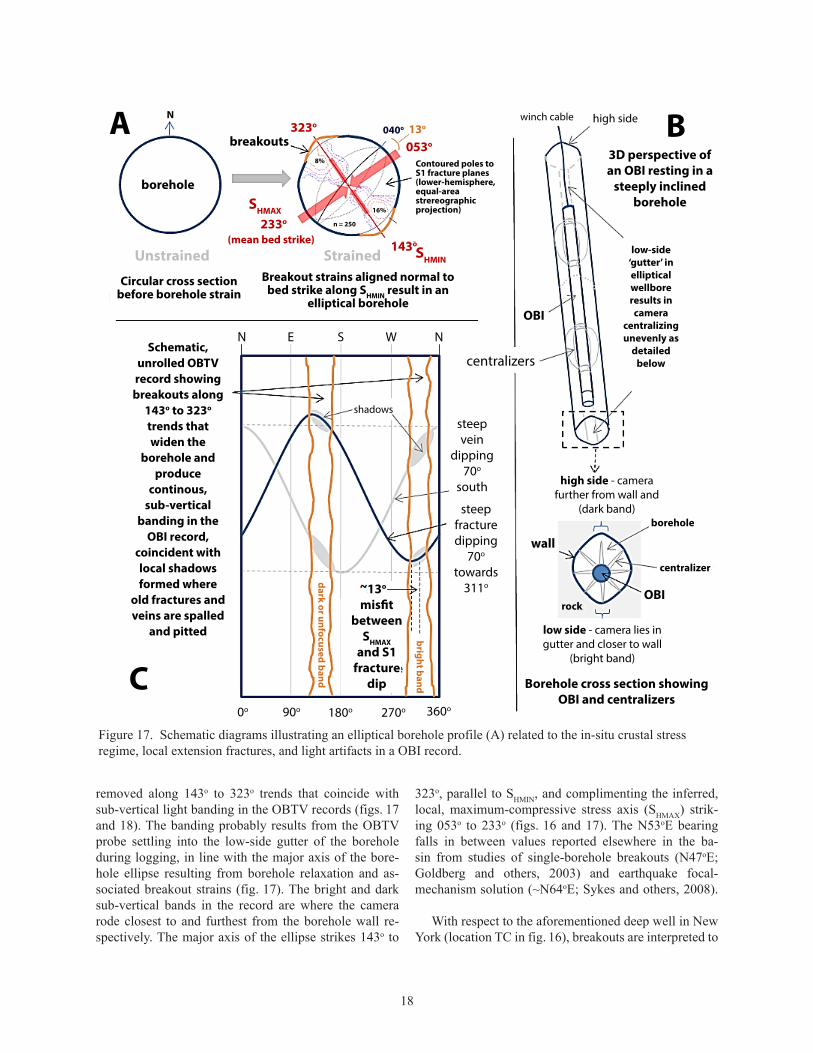
removed along 143o to 323o trends that coincide with sub-vertical light banding in the OBTV records (figs. 17 and 18). The banding probably results from the OBTV probe settling into the low-side gutter of the borehole during logging, in line with the major axis of the bore-hole ellipse resulting from borehole relaxation and as-sociated breakout strains (fig. 17). The bright and dark sub-vertical bands in the record are where the camera rode closest to and furthest from the borehole wall re-spectively. The major axis of the ellipse strikes 143o to

18

A

C

B

A B

C

N

borehole

breakouts

Unstrained Strained

SHMAX

233o

(mean bed strike) 143oSHMIN

323o

053o

040o 13o

8%

n = 250

16%

Contoured poles toS1 fracture planes(lower-hemisphere,equal-areastrereographicprojection)

Circular cross section before borehole strain

Breakout strains aligned normal to bed strike along SHMIN result in an

elliptical borehole

winch cable high side

3D perspective of an OBI resting in a

steeply inclined borehole

low-side ‘gutter’ in elliptical wellbore results in camera

centralizing unevenly as

detailed below

OBI

high side - camera further from wall and

(dark band)

centralizers

wall

OBI

borehole

centralizer

rock

low side - camera lies in gutter and closer to wall

(bright band)

Borehole cross section showing OBI and centralizers

Schematic, unrolled OBTV record showing breakouts along

143o to 323o trends that widen the

borehole and produce

continous, sub-vertical

banding in the OBI record,

coincident with local shadows formed where

old fractures and veins are spalled

and pitted

N NE S W

shadows

13o mis�t

between SHMAX

and S1 fracture

dip

0o 90o 180o 270o 360o

dark or unfocused band

bright band

steep vein

dipping 70o

south

steep fracture dipping

70o towards

311o

Figure 17. Schematic diagrams illustrating an elliptical borehole profile (A) related to the in-situ crustal stressregime, local extension fractures, and light artifacts in a OBI record.

323o, parallel to SHMIN, and complimenting the inferred, local, maximum-compressive stress axis (SHMAX) strik-ing 053o to 233o (figs. 16 and 17). The N53oE bearing falls in between values reported elsewhere in the ba-sin from studies of single-borehole breakouts (N47oE; Goldberg and others, 2003) and earthquake focal-mechanism solution (~N64oE; Sykes and others, 2008). With respect to the aforementioned deep well in New York (location TC in fig. 16), breakouts are interpreted to

19

have trends and widths differing as a function of depth and crustal anisotropy, with observed breakouts ranging from ~N80o E to N25oE and reflecting a clockwise twist of the current principal stress axis progressing upward, through the Late Triassic section. This range falls into the envelope of “all plausible orientations of the maximum horizontal compressive stress axis (SHMAX) in the region” of N10oE to E-W (Zhakarova and Goldberg, 2014). It is simply noted here that the upward twist of 54o clockwise of the principal stress axes through the Late Triassic sec-tion is of opposite polarity but the same magnitude as the upward 60o twist of the finite-stretching direction revealed by sets of overlapping, old tensile-transitional shear fractures occurring in basin strata (Herman, 2009). These systematic fractures cluster into three promi-nent strike sets correlated to early- (S1, about 30oE to N60oE), intermediate- (S2, about N15o to N30oE), and

late-stage (S3, about N-S) stretching events in the basin (fig. 16). They display progressive linkage, spatial clus-tering, and geometric interactions pointing to succes-sive, heterogeneous crustal stretching and the progres-sive development of major fault blocks resulting from complex dip-slip and oblique-slip strains. The geometry, distribution, and morphology of the extension fractures indicate progressive counterclockwise rotation of the re-gional, principal extension axis from NW-SE during and after deposition of Late Triassic strata (Herman, 2009).

The mean strike of the oldest, tensile-transitional frac-ture group (~N40oE with dip azimuth ~310o) varies only about 13o counterclockwise from SHMAX inferred here (N53oE), but falls neatly in the 30o envelope of shear-failure varying about SHMAX predicted for rocks follow-ing Coulomb fracture criterion under compressive strain

6.2,149.1,265,6,,Vein,,,

6.1,149.5,15,15,8,Vein,,,

6.3,145.3,341,11,,Vein,,,

6.3,146.9,63,6,,Vein,,,

6.3,148,145,36,18,Vein,,,

6.2,147.8,343,15,,Fracture,,

6.2,146.6,132,14,,Fracture,,

6.2,147.8,340,22,,Fracture,,

6.2,146.7,342,11,,Vein,,,

6.3,148.5,131,19,31,Vein,,,

5.3,143.5,39,1,,Vein,,,

5.6,143.8,302,13,,Vein,,,

5.6,143.8,95,6,,Vein,,,

5.3,148.3,292,43,,Vein,,,

5,144.7,127,35,,Vein,,,

4.9,146,120,32,,Vein,,S,

4.9,147.3,64,7,,Vein,,S,

4.8,145.7,312,76,,Vein,,,

4.5,148.4,300,16,,Vein,,,

4.6,148.9,138,20,,Vein,,,

4.7,148,128,68,,Vein,,,

4.4,146.1,326,11,,Vein,,,

4.6,147.6,128,8,,Vein,,,

4.6,145.5,310,78,,Vein,,,

5.3,144.6,292,9,,Vein,,,

5.3,145.5,351,9,,Vein,,,

0o 90o 180o 270o 0o 315o 135o0o 90o 180o 270o 0o 315o 135o

370.0

371.0

372.0

373.0

374.0

375.0

376.0

377.0

378.0

655.0

656.0

657.0

658.0

659.0

660.0

661.0

662.0

663.0

664.0

OBI banding above waterblurry light

OBI banding below waterdark light

Figure 18. Sections of the EG1 OBI record showing light artifacts centered on 140o and 320o trends.

(Fossen, 2010). This simply means that old tensile frac-tures oriented less than 30o strike from SHMAX are current-ly prone to reactivated slip as they are suitably aligned sub-parallel to the minimum, horizontal compressive stress axis to be propped open (SHMIN, figs. 16 and 17). Moreover, both S1 and S2 fracture groups mapped in the basin fall inside this fracture envelope, but S1 fractures are the only extension-fracture group represented within

the lower section of the Passaic Formation here, and Eliz-abeth is far removed from intrabasinal faults of S2 ori-entation (fig. 1). Having S1 fractures in this stratigraphic interval at this place in the basin is consistent with having the earliest, S1 fractures occurring in Late Triassic mud rocks throughout the basin, whereas those of later fracture groups are abundant in mid-to upper sections of the Pas-saic Formation and Early Jurassic strata (Herman, 2009).

This work upholds some long-held views of basin geology while refining others. For example, the hori-zontal drift of EG1 generally opposes bed dip (~323o) along the inferred 143o bearing of SHMIN. Therefore, stratigraphic tilt primarily determines both the hemi-sphere and direction in which boreholes drift off verti-cal, with boreholes curving gently down section in a direction lying normal to the bed plane. As previously mentioned, Zhakarova and Goldberg (2014) observed a clockwise rotation of the in situ stress axes in strata penetrated by the Tri-Carb well that reflects systematic variations in fracture strike and formation anisotropy with depth. This brings us to a couple of final points. Acoustic and optical BTV work is commonly used for groundwater studies in bedrock having boreholes open to depths less than 600 ft (183 m). Deeper holes drilled for hydrocarbon exploration or reservoir char-acterization principally rely on high-resolution electri-cal methods or sonic systems. When BTV is used, it is more common to see only one type of record col-lected because it more than doubles the cost of a proj-ect to process, interpret, and compare the results for each type of record. Acoustic BTV methods are com-monly favored over optical ones when investigating deep boreholes such as these because water turbidity is difficult to prevent or mitigate and sections become obscured in optical BTV records as seen in figure 4, resulting in incomplete geological interpretations. But

DISCUSSION

acoustic BTV signals cannot always differentiate com-pletely healed (mineralized) fractures from host rock, and can thereby lead to a fracture inventory that is bi-ased towards those that are suitably aligned to sustain breakout strains that enhance their acoustic signal. Based on the findings of this optical study, old, formerly mineralized fractures are apparently rejuve-nated with structural slip and have effective porosity at great depths when they strike acutely to SHMAX. The fault slip noted on S1 fractures where they apparently cross cut and offset the sub-horizontal gypsum veins (fig. 11) merits further study because to date, this is the only place that we have seen this relationship. It re-mains unclear whether the small slip strains observed on these old fractures results from recent, concurrent vein growth on both fracture sets or if the late slip on the steeply dipping S1 fractures is strictly younger than the sub-horizontal veining. In either case, these strains are among the latest strains observed in the region, and they probably reflect recent brittle strain responses to crustal loading and unloading. Nevertheless, in or-der to establish a viable hydrogeologic framework, it is very important to be able to recognize old fractures from new, regardless of the instrumentation used, in order to help predict how the various primary and sec-ondary geological features interact in the contemporary crustal stress field to store and channel groundwater.

We thank Harry and Mark Sussman and Chuck Van der Volgen of Earth Tech Energy Solutions for the opportunity to obtain an unprecedented, deep look into the properties of the Brunswick aquifer in an urban environment. It was a pleasure having Jack Koczan of The Verina Group involved through-out the borehole logging as a representative of Earth Tech. I especially thank Irving “Butch” Grossman,

Otto Zapecza, William Graff, and Kathleen Vandegrift for their editorial and production assistance. We also thank Jim Peterson of Princeton Geosciences, LLC for his editorial review and comments to early forms of the manuscript. We also thank Brad Posner of Pet-roPhysicsPlus Consulting for multimedia files illus-trating borehole breakouts in optical BTV images of deep wells from the Marcellus Shale in Pennsylvania.

ACKNOWLEDGEMENTS

20

21

Drake, A. A., Jr., Volkert, R.A., Monteverde, D.H., Herman, G.C., Houghton, H.H., and Parker, R.A., 1996, Bedrock geologic map of northern New Jersey: U.S. Geological Survey Miscellaneous Investigation Series Map I-2540-A, scale 1:100,000; 2 sheets.

Fossen, Haakon, 2010, Structural Geology, Cambridge University Press, Cambridge, UK, 480 p.

Goldberg, D.S., Lupo, T., Caputi, M., Barton, C., and Seeber, L., 2003, Stress regimes in the Newark Basin rift: evidence from core and downhole data, in The great rift valleys of Pangea in eastern North Ameri-ca, 1, p. 104-117.

Herman, G. C., 2001, Hydrogeological framework of bedrock aquifers in the Newark Basin, New Jersey: in LaCombe, P.J. and Herman, G.C., eds. Geology in Service to Public Health, Field Guide and Proceed-ings of the 18th Annual Meeting of the Geological Association of New Jersey, p. 6-45.

Herman, G. C., 2005, Joints and veins in the Newark basin, New Jersey, in regional tectonic perspective: in Gates, A. E., ed., Newark basin – View from the 21st

Century: Field Guide and Proceedings of the 22nd An-nual Meeting of the Geological Association of New Jersey, p. 75-116.

Herman, G. C., 2009, Steeply-dipping extension frac-tures in the Newark basin, Journal of Structural Geol-ogy, v. 31, p. 996-1011.

Herman, G.C., 2010, Hydrogeology and borehole geophysics of fractured-bedrock aquifers, in Her-man, G.C., and Serfes, M.E., eds., Contributions to the geology and hydrogeology of the Newark basin: N.J. Geological Survey Bulletin 77, Chapter F., p. F1-F45.

Herman, G. C., 2013, Utilizing Google Earth for geospatial, tectonic, and hydrogeological research at the New Jersey Geological Survey: Geological Society of America, Abstracts with Programs v. 45, No. 1. www.impacttectonics.org/gcherman/down-loads/GEO310/GCH_GESymbols/GCH_GE_Geol-ogy_Apps.htm

Herman, G.C., and Curran, J., 2010, Borehole geophys-ics and hydrogeology studies in the Newark basin,

New Jersey (38 MB PDF), in Herman, G.C., and Serfes, M.E., eds., Contributions to the geology and hydrogeology of the Newark basin: N.J. Geological Survey Bulletin 77, Appendixes 1-4, 245 p.

Herman, G. C., Canace, R.J., Stanford, S.D., Pristas, R.S., Sugarman, P.J., French, M.A., Hoffman, J.L., Serfes, M.S., and Mennel, W.J., 1998, Aquifers of New Jersey (2 MB PDF): N. J. Geological Survey Open-File Map 24, scale 1:500,000, 1 sheet.

Herman, G.C., Santangelo, A., and Vandegrift, K., 2012, Geothermal parameters required for the design and installation of geothermal heat-pump systems in New Jersey: N.J. Geological and Water Survey Newsletter, Unearthing New Jersey, v. 8, no. 2, p. 4-6.

Holcombe, R. J., 2004, GEOorient 9.2 Stereographic projections and rose diagram plots: Personal com-puter software downloaded from www.earth.uq.edu.au/~rodh/software, Queensland, Australia.

Kirvan, A. P., (1997), Latitude/Longitude, NCGIA Core Curriculum in GIScience, http://www.ncgia.ucsb.edu/giscc/units/u014/u014.html.

Michalski, A., and Britton, R., 1997, The role of sedi-mentary bedding in the hydrogeology of sedimentary bedrock - Evidence from the Newark Basin, New Jersey: Ground Water, v. 35, no. 2, p. 318-327.

Olsen, P. E., Kent, D. V., Cornet, B., Witte, W. K., and Schlische, R. W., 1996, High-resolution stratigraphy of the Newark rift basin (early Mesozoic, eastern North America): Geological Society of America Bul-letin, v. 108, no. 1, p. 40-77.

Parnell, J., and Monson, B., 1995, Paragenesis of hy-drocarbon, metalliferous and other fluids in NewarkGroup basins, Eastern U.S.A., Institute of Mining and Metallurgy, Transactions, Section B: Applied Earth Science; v. 104, p. 136-144.

Simonson, B. M., Smoot, J. P., and Hughes, J. L., 2010, Authigenic minerals in macropores and veins in Late Triassic mudstones of the Newark basin: Implications for fluid migration through mudstone, in Herman, G.C., and Serfes, M.E., eds., Contributions to the geol-ogy and hydrogeology of the Newark basin: N.J. Geo-logical Survey Bulletin 77, Chapter B, p. B1-B26.

REFERENCES

Smoot, J. P., and Olsen, P. E., 1985, Massive mud-stones in basin analysis and paleoclimatic inter-pretation of the Newark Supergroup, in Robinson, G. R., and Froelich, A. J., eds., Proceedings of the second U.S. Geological Survey workshop on the Early Mesozoic basins of the Eastern United States: U. S. Geological Survey Circular 946, p. 29-33.

Smoot, J. P., and Olsen, P. E., 1988, Massive mud-stones in basin analysis and paleoclimatic interpre-tations, in Manspeizer, W., ed., Triassic-Jurassic rifting, continental breakup, and the origin of the Atlantic Ocean and passive margins, Part A: Am-sterdam, Netherlands, Elsevier, p. 249-274.

Smoot, J. P., and Olsen, P.E., 1994, Climatic cycles as sedimentary controls of rift-basin lacustrine depos-its in the early Mesozoic Newark Basin based on continuous core, in Lomando, T., and Harris, M., eds. Lacustrine depositional systems: Society of Economic Paleontologists and Mineralogists Core Workshop Notes, v. 19, p. 201-237.

Stanford, S. D., 1995, Surficial geology of the JerseyCity Quadrangle, Hudson and Essex Counties, New Jersey: New Jersey Geological Survey Open-fileMap OFM 20, scale 1:24,000.

Sykes, L. R., Armbruster, J. G., Kim, W-Y., and Seeber, L., 2008, Observations and tectonic setting of the historic and instrumentally located earthquakes in the greater New York City-Philadelphia area: Bul-letin of the Seismological Society of America, v. 98, no. 4, p. 1696-1719.

Tabakh, M. El, Schreiber, B. C., and Warren, J. K., 1998, Origin of fibrous gypsum in the Newark riftBasin, eastern North America: Journal of Sedimen-tary Research, v. 68, p. 88-99.

Van Houten, F. B., 1965, Composition of Triassic Lockatong and associated formations of Newark Group, central New Jersey and adjacent Pennsylva-nia: American Journal of Science, v. 263, p. 825-8631.

Zakharova, N. V., and Goldberg, D. S., 2014, In situ stress analysis in the northern Newark Basin: Impli-cations for induced seismicity from CO2 injection: Journal of Geophysical Research of the Solid Earth, v. 199, doi:10.1002/2013JB010492.

Zoback, M. D., 2010, Reservoir Geomechanics: Cam-bridge University Press, Cambridge, U.K.

22

APPENDIX 1. SUPPORT INFORMATION ABOUT THE NJ GEOLOGICAL AND WATER SURVEY BOREHOLE TELEVIEWER AND HEAT-PULSE

FLOW-METER INSTRUMENTS AND METHODS

A. Advanced Logic Technologies’ OBI40 Digital Optical Borehole Imaging Tool

The borehole televiewer (BTV) instrument used by the NJ Geological and Water Survey is an Ad-vanced Logic Technology (ALT) Optical Borehole Imager (OBI) Model OBI40 (A). It is a slimhole logging tool designed for the optical imaging of the borehole walls of open and cased wells, either in air or clean water. It includes a high precision de-viation sensor allowing accurate orientation of the image and borehole. The purpose of the tool is to provide detailed, oriented, structural and geologi-cal information. The OBI incorporates a high reso-lution, high sensitivity CCD camera that captures successive digital snapshots of the borehole wall that are stacked for display and geological analy-sis. Light from an LED light source located below the camera and above a conical mirror is directed off the borehole wall, through a clear window, and upward to the camera that includes an array of light sensors. Azimuthal resolutions are 720 pixels, or more commonly, 360 pixels per inch. By using pro-cessed camera data in combination with deviation sensor data, the tool can generate an unwrapped 360o oriented image (B) of the borehole walls.

A

B

23

B. OBI Data Processing

The OBI produces a continuous, oriented, digi-tal photographic image of the borehole walls using magnetic north as a reference azimuth. A digital re-cord typically includes a small number of data errors, or record omissions that are mm-scale, bad traces that failed to upload or process depending upon log-ging speeds and environmental conditions. They ap-pear as thin white lines spaced at various depths in the pre-processed borehole image. WellCAD® was used to interpolate across bad traces resulting in a continuous, uninterrupted image. Data-processing procedures for each OBI record are detailed in the log header, as detailed in the next section below.Prior to structural interpretation, an acquired im-age of an approximately cylindrical borehole is ‘unrolled’ and rotated to true north (~12.5o coun-terclockwise rotation in New Jersey) using the bore-hole-telemetry parameters derived from incremen-tally comparing the instruments varying position in a borehole (tilt and tilt bearing) with respect the Earth’s gravitational and magnetic potential fields. Below

is a schematic diagram illustrating how simple in-clined planes intersect cylindrical boreholes and how 3-dimensional BTV records are transformed or ‘unrolled’ into 2-dimensional arrange-ment for interpretation of the geological planes.

GEOrient v.9.2 is used to plot and analyze the structural data. Feature (plane) orientations are plot-ted for each structure type using circular histograms and equal-angle, lower hemisphere stereonet dia-grams. Stereonet analyses commonly included den-sity contours of poles-to-planes to derive representa-tive planes, and plane cyclographic plots of primary stratigraphic layering and secondary fractures, veins, cleavage, and fault planes. OBI-40 records produced by the NJGWS are currently output as Adobe Portable Document Files (PDF) files formatted in standard page layout that is 8.5 inches wide by 11 inches long, or up to 200 inches long for continuous representation and/or printing. The latter format outputs about 360 feet of borehole record per 200 inches page at the 1:20 scale.

24

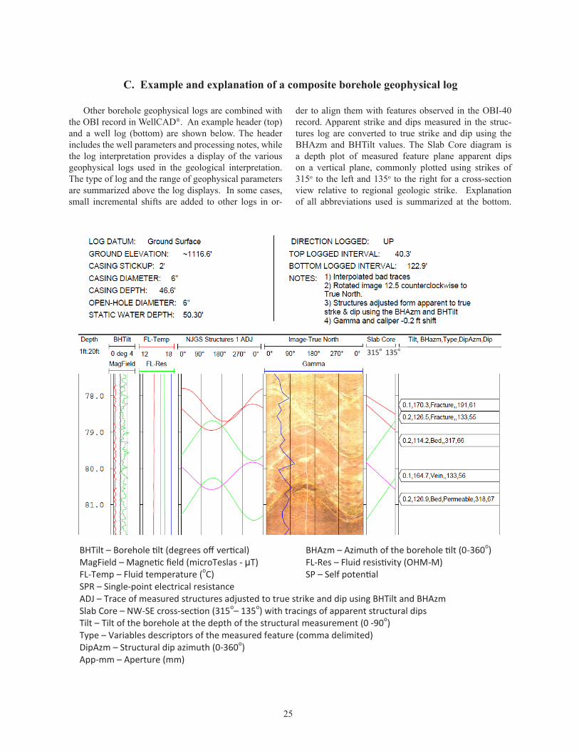
Other borehole geophysical logs are combined with the OBI record in WellCAD®. An example header (top) and a well log (bottom) are shown below. The header includes the well parameters and processing notes, while the log interpretation provides a display of the various geophysical logs used in the geological interpretation. The type of log and the range of geophysical parameters are summarized above the log displays. In some cases, small incremental shifts are added to other logs in or-

C. Example and explanation of a composite borehole geophysical log

der to align them with features observed in the OBI-40 record. Apparent strike and dips measured in the struc-tures log are converted to true strike and dip using the BHAzm and BHTilt values. The Slab Core diagram is a depth plot of measured feature plane apparent dips on a vertical plane, commonly plotted using strikes of 315o to the left and 135o to the right for a cross-section view relative to regional geologic strike. Explanation of all abbreviations used is summarized at the bottom.

BHTilt – Borehole tilt (degrees off vertical) BHAzm – Azimuth of the borehole tilt (0-360o) MagField – Magnetic field (microTeslas - µT) FL-Res – Fluid resistivity (OHM-M) FL-Temp – Fluid temperature (oC) SP – Self potential SPR – Single-point electrical resistance ADJ – Trace of measured structures adjusted to true strike and dip using BHTilt and BHAzm Slab Core – NW-SE cross-section (315o– 135o) with tracings of apparent structural dips Tilt – Tilt of the borehole at the depth of the structural measurement (0 -90o) Type – Variables descriptors of the measured feature (comma delimited) DipAzm – Structural dip azimuth (0-360o) App-mm – Aperture (mm)

315o 135o

25

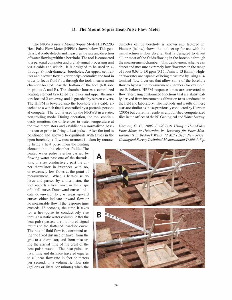
D. The Mount Sopris Heat-Pulse Flow Meter

The NJGWS uses a Mount Sopris Model HFP-2293 Heat-Pulse Flow Meter (HPFM) shown below. This geo-physical probe detects and measures the rate and direction of water flowing within a borehole. The tool is connected to a personal computer and digital-signal processing unit via a cable and winch. It is designed to be used in 4- through 8- inch-diameter boreholes. An upper, central-izer and a lower flow diverter helps centralize the tool in order to focus fluid flow through the tools measurement chamber located near the bottom of the tool (left side in photos A and B). The chamber houses a centralized heating element bracketed by lower and upper thermis-tors located 2 cm away, and is guarded by screen covers. The HPFM is lowered into the borehole via a cable at-tached to a winch that is controlled by a portable person-al computer. The tool is used by the NJGWS in a static, non-trolling mode. During operation, the tool continu-ously monitors the differences in water temperature at the two thermistors and establishes a normalized base-line curve prior to firing a heat pulse. After the tool is positioned and allowed to equilibrate with fluids in the open borehole, a flow measurement is taken by remote-ly firing a heat pulse from the heating element into the chamber fluids. The heated water pulse is either carried by flowing water past one of the thermis-tors, or rises conductively past the up-per thermistor in instances with no, or extremely low flows at the point of measurement. When a heat-pulse ar-rives and passes by a thermistor, the tool records a heat wave in the shape of a bell curve. Downward curves indi-cate downward flo , whereas upward curves either indicate upward flow or no measurable flow if the response time exceeds 32 seconds, the time it takes for a heat-pulse to conductively rise through a static water column. After the heat-pulse passes, the monitored signal returns to the flattened, baseline curve. The rate of fluid flow is determined us-ing the fixed distance of travel from the grid to a thermistor, and from measur-ing the arrival time of the crest of the heat-pulse wave. The heat-pulse ar-rival time and distance traveled equates to a linear flow rate in feet or meters per second, or a volumetric flow rate (gallons or liters per minute) when the

diameter of the borehole is known and factored in. Photo A (below) shows the tool set up for use with the manufacturer’s flow diverter that is designed to divert all, or most of the fluids flowing in the borehole through the measurement chamber. This deployment scheme can detect and measure extremely low flow rates in the range of about 0.03 to 1.0 gpm (0.15 ft/min to 13 ft/min). High-er flow rates are capable of being measured by using cus-tomized flow diverters that allow some of the borehole flow to bypass the measurement chamber (for example, see B below). HPFM response times are converted to flow rates using customized functions that are statistical-ly derived from instrument-calibration tests conducted in the field and laboratory. The methods and results of these tests are similar as those previously conducted by Herman (2006) but currently reside as unpublished computerized files in the offices of the NJ Geological and Water Survey.

Herman, G. C., 2006, Field Tests Using a Heat-Pulse Flow Meter to Determine its Accuracy for Flow Mea-surements in Bedrock Wells (2 MB PDF): New Jersey Geological Survey Technical Memorandum TM06-1, 8 p.

B

A

26

APPENDIX 2. NJGWS STRUCTURAL PLANES AND BOREHOLE TELEMETRY PARAMETERS FOR THE EG1 AND EG20 OBI-40 RECORDS

27

Digital-data file download using a compressed-file format (GSR42.zip) containing the following files:

• NJGWS GSR42 Borehole EG1_1773_UP360c.pdf (3.69 MB) - Adobe Systems Incorporated©,Adobe Portable Document File (PDF) of interpreted OBI-40 record of borehole EG1

• NJGWS GSR42 Borehole EG20_1426_UP360c.pdf (1.98 MB) - Adobe Systems Incorporated©,Adobe Portable Document File (PDF) of interpreted OBI-40 record of borehole EG20

• NJGWS GSR42 - Elizabeth Geothermal.kmz (123 KB) - Google Inc.©, Google Earth Keyhole Markup Language (KMZ) 3D model with OBI-40 structural interpretations of boreholes EG1 and EG20 including geophysical logs.

• NJGWS GSR42 Appendix2.xlsx - Microsoft Excel® (2010) workbook containing worksheets forborehole EG1 and EG20, including depth, telemetry, and structural-feature parameters measuredin the OBI-40 records