NISSUNA UMANA INVESTIGAZIONE SI PUO DIMANDARE VERA SCIENZIAS’ESSA NON PASSA PER LE MATEMATICHE DIMOSTRAZIONI

LEONARDO DAVINCI

Mathematics and Mechanicsof

Complex Systems

msp

vol. 4 no. 2 2016

MICKHAIL A. GUZEV AND ALEXANDR A. DMITRIEV

STABILITY ANALYSIS OF TWO COUPLED OSCILLATORS

MATHEMATICS AND MECHANICS OF COMPLEX SYSTEMSVol. 4, No. 2, 2016

dx.doi.org/10.2140/memocs.2016.4.139MM ∩

STABILITY ANALYSIS OF TWO COUPLED OSCILLATORS

MICKHAIL A. GUZEV AND ALEXANDR A. DMITRIEV

We study a system of two coupled oscillators linked by a linear elastic springand positioned vertically in a uniform gravity field. It is demonstrated that thesystem has different equilibrium configurations below and above the oscillators’suspension centers. We obtained the relations of the string stiffness and thedistance between the suspension centers identifying the stability region of theoscillators.

1. Introduction

Mechanical oscillators are models of various physical processes and complex phys-ical systems as demonstrated by a vast body of literature. For example, coupledoscillators are used to describe the lattice vibrations in crystals [Kittel 2005].

A well-known and useful oscillator system is the sympathetic oscillators [Som-merfeld 1994], which are two linked oscillators with equal rods and masses inter-acting through a spring. Small linear oscillations about the equilibrium point havebeen studied, focusing on analyzing the physical situations depending on the springstiffness.

There have been many scientific studies on oscillating dynamics of mechanicalsystems. However, new results still periodically appear. For instance, Maianti et al.[2009] study the impact of symmetrical initial conditions of linked oscillators ina uniform gravity field on the eigenoscillations and obtain the initial angle thatensures an independent frequency spectrum. Ramachandran et al. [2011] deal withdifferent configurations of two pendulums connected by a rod. The results are thatthere are stable equilibrium configurations that are asymmetrical with respect tothe vertical midline. An important property of the system is that there can appearbifurcations depending on the distance between the suspension points. The ob-tained results are useful for investigation of the pantographic structures [dell’Isolaet al. 2016]. The interest in these materials is defined by development of the three-dimensional printing technology. They can be regarded as families of pendulums(also called fibers) interconnected by pivots in equilibrium. Synchronization of

Communicated by Francesco dell’Isola.MSC2010: 70E55, 70H14.Keywords: coupled oscillators, equilibrium configurations, stability, linear interaction.

139

140 MICKHAIL A. GUZEV AND ALEXANDR A. DMITRIEV

two oscillators is the focus of [Koluda et al. 2014] and their chaotic dynamics isstudied in [Huynh and Chew 2010; Huynh et al. 2013].

A system of inverted oscillators also provides physically sound phenomena. Sta-ble positions can also be attained if there is a fast perturbation frequency [Stephen-son 1908]. This result is due to Pyotr Kapitza [Kapitza 1951a; Kapitza 1951b].A more accurate condition of dynamical stabilization of an inverted oscillator isintroduced in [Butikov 2011]. Chelomei’s problem of the stabilization of an elas-tic, statically unstable rod by means of a vibration is considered in [Seyranianand Seyranian 2008]. The stability of two inverted linearly linked oscillators isanalyzed in [Markeev 2013]. The author reveals bifurcations depending on thelinking spring stiffness and single out parameters that lead to stable or unstableequilibria. The phenomenon of stabilization by parametric excitation of an elasti-cally restrained double inverted pendulum is considered in [Arkhipova et al. 2012].The problem of restabilization of statically unstable linear Hamiltonian systemsis analyzed in [Arkhipova and Luongo 2014]. A comprehensive review of thedynamics of a large number of coupled oscillators is presented in [Pikovsky andRosenblum 2015].

The objective of the current paper is to study the stability of the model of twolinearly interacting oscillators in a uniform gravity field. The formal analysis ofequilibrium stability is carried out in the framework of the linear stability approach.It consists of determination of the equilibrium position and calculation of the matrixof the second partial derivatives of potential energy in the equilibrium position. Ifthe matrix spectrum is positive, the equilibrium is stable. Otherwise, it is unstable.We focus on analyzing the equilibrium solutions depending on the distance betweenthe suspension points and the spring stiffness. This analysis includes differentconfigurations of the model of coupled oscillators.

2. Basic equations

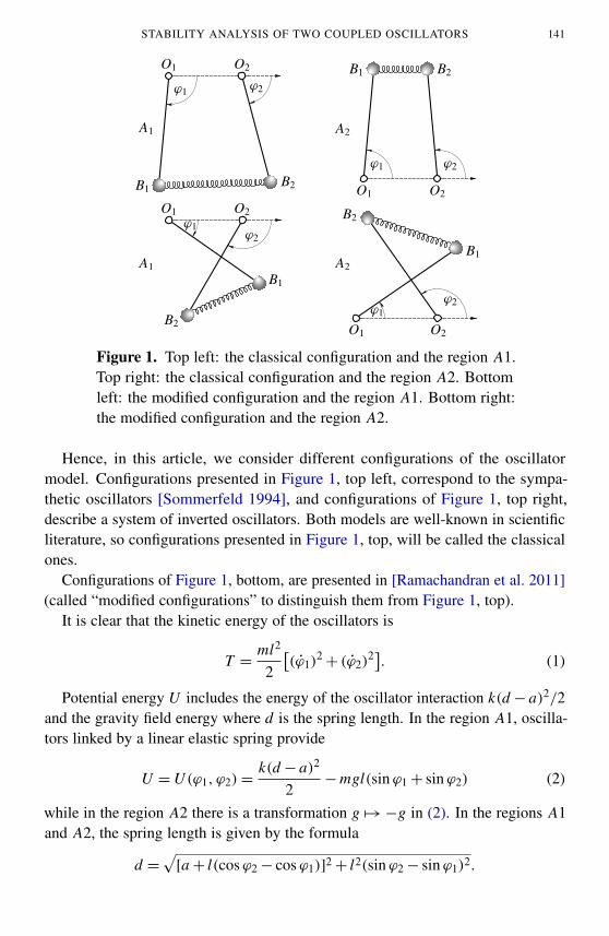
Let us consider two oscillators of length l and mass m in a uniform gravity field.We assume that the suspension points O1 and O2 are positioned on a motionlesshorizontal straight line, while the distance between the suspension points a is con-stant. A massless elastic spring of stiffness k links the masses at points B1 and B2,which coincide with the masses’ positions. We assume that the oscillators move ina fixed vertical plane containing the interval O1O2 (see Figure 1). The oscillatorscan be situated both below the horizontal suspension line (see the region A1 inFigure 1, left) and above it (see the region A2 in Figure 1, right). In the region A1,angles ϕ1 and ϕ2 lie in the interval (0, π), while transition to the region A2 impliesthe transformation ϕ1, ϕ2 7→ −ϕ1,−ϕ2.

STABILITY ANALYSIS OF TWO COUPLED OSCILLATORS 141

O1 O2

ϕ1 ϕ2

A1

B1 B2

B1 B2

A2

ϕ1 ϕ2

O1 O2

O1 O2ϕ1

ϕ2

A1

B2

B1

B2

B1A2

O1 O2

ϕ1ϕ2

Figure 1. Top left: the classical configuration and the region A1.Top right: the classical configuration and the region A2. Bottomleft: the modified configuration and the region A1. Bottom right:the modified configuration and the region A2.

Hence, in this article, we consider different configurations of the oscillatormodel. Configurations presented in Figure 1, top left, correspond to the sympa-thetic oscillators [Sommerfeld 1994], and configurations of Figure 1, top right,describe a system of inverted oscillators. Both models are well-known in scientificliterature, so configurations presented in Figure 1, top, will be called the classicalones.

Configurations of Figure 1, bottom, are presented in [Ramachandran et al. 2011](called “modified configurations” to distinguish them from Figure 1, top).

It is clear that the kinetic energy of the oscillators is

T =ml2

2

[(ϕ1)

2+ (ϕ2)

2]. (1)

Potential energy U includes the energy of the oscillator interaction k(d − a)2/2and the gravity field energy where d is the spring length. In the region A1, oscilla-tors linked by a linear elastic spring provide

U =U (ϕ1, ϕ2)=k(d − a)2

2−mgl(sinϕ1+ sinϕ2) (2)

while in the region A2 there is a transformation g 7→ −g in (2). In the regions A1and A2, the spring length is given by the formula

d =√[a+ l(cosϕ2− cosϕ1)]2+ l2(sinϕ2− sinϕ1)2.

142 MICKHAIL A. GUZEV AND ALEXANDR A. DMITRIEV

It is interesting that there is a natural geometrical condition for the configurations.In the case of the classical configurations (Figure 1, top), the difference of the rodlength projections on the suspension axis is less then a, giving the condition

l(cosϕ1− cosϕ2) < a. (3)

In the case of the modified configurations (Figure 1, bottom), the correspondingdifference is larger than a:

l(cosϕ1− cosϕ2) > a. (4)

From (1) and (2), the Lagrangian of the system ensures

L = T −U =ml2

2(ϕ2

1 + ϕ22)−

k(d − a)2

2+ 2mgl sin

ϕ1+ϕ2

2cos

ϕ1−ϕ2

2. (5)

Now let us introduce instead of ϕ1 and ϕ2 new coordinates q1 and q2, whereq1 = (π −ϕ1−ϕ2)/2 and q2 = (ϕ1−ϕ2)/2. Introducing new dimensionless timeτ = t√

2g/ l and Lagrangian 3= L/mgl, (5) can be rewritten as

3= 12(q

21 + q2

2 )−5(q1, q2),

5=5(q1, q2)=(s−µ)2

2ν− cos q1 cos q2,

s2= sin2 q2+ 2µ cos q1 sin q2+µ

2, µ=a2l, ν =

2mglk

.

(6)

Parameter ν characterizes the relation between the potential energy of the oscilla-tors and the spring’s effective energy, while µ is a kinematic parameter and dependson the metric characteristics.

Differential equations of the oscillator dynamics in the form of Lagrangian equa-tions are

ddτ∂3

∂qi=∂3

∂qi⇐⇒ qi =−

∂5

∂qi, i = 1, 2. (7)

System (7) allows for solutions corresponding to both the classical and the modifiedconfigurations. Therefore, while analyzing system (7), it is necessary to point outthe region of feasible solutions. Conditions (3)–(4) can be written as

µ+ cos q1 sin q2 > 0, (8)

µ+ cos q1 sin q2 < 0. (9)

Equilibrium configurations of the oscillator system ensue from the conditionqi = 0; then it follows from (7) that they are determined as the critical points ofthe system’s potential energy

∂5

∂q1= 0,

∂5

∂q2= 0. (10)

STABILITY ANALYSIS OF TWO COUPLED OSCILLATORS 143

O1 O2

B2 B1

ν

ν(µ)

� %(µ)

µ∗

µ∗

µ

1.0

0.9

0.8

0.7

0.6

0.5

0.4

0.3

0.2

0.1

0 0.1 0.2 0.3 0.4 0.5 0.6 0.7 0.8 0.9 1.0

Figure 2. Left: the modified symmetric equilibrium configurationfor the oscillator model in the region A1. Right: the stability do-main � for the modified configuration in the region A1.

Taking into account (6), one can rewrite (10) in the form

sin q1

[(µs− 1

)µ sin q2+ ν cos q2

]= 0, (11)(

1−µ

s

)(sin q2+µ cos q1) cos q2+ ν cos q1 sin q2 = 0. (12)

Thus, by solving the system (11)–(12), one obtains a set of equilibrium configura-tions.

3. Symmetrical equilibrium configurations

Symmetrical configurations are characterized by symmetrical positions of the pen-dulums with respect to the vertical midline. The classical symmetric configurationsin the region A1 follow from q1 = 0, while in the region A2 from q1 = π . In thiscase, (11) is satisfied identically (sin q1 = 0); then the distance (6) between theoscillators equals s=|sin q2±µ| and the condition (8) is equivalent to µ±sin q2>0,i.e., s = µ± sin q2. So (12) reduces to sin q2(cos q2± ν)= 0, which was studiedin [Markeev 2013].

The modified symmetrical configurations in the region A1 follow from ϕ2 =

π−ϕ1, q1= 0, and are shown in Figure 2. This allows us to rewrite the condition (9)as µ+ sin q2 < 0, i.e., µ < 1 and |q2|< π/2; then the distance s =−(µ+ sin q2)

and (12) is equivalent to

(2µ+ sin q2) cos q2+ ν sin q2 = 0⇐⇒ sin 2q2+ 2

√4µ2+ ν2 sin(q2− q∗)= 0, (13)

144 MICKHAIL A. GUZEV AND ALEXANDR A. DMITRIEV

where q∗=− arcsin(2µ/√

4µ2+ ν2). Let q∗∗=− arcsinµ; then inside the interval(q∗, q∗∗), (13) has a unique solution q provided the inequality

ν <√

1−µ2, µ < 1, (14)

is true. Indeed, (13) is identical to

2µ+ sin q2 =−ν tan q2. (15)

The right-hand side of (15) decreases; it equals 2µ/ν at point q∗ and µ/√

1−µ2 atpoint q∗∗. The left-hand side increases; it is less than 2µ/ν at point q∗ and equals2µ/ν at point q∗∗. If the inequality (14) is satisfied, the function graphs intersectat one and only one point q .

Let us analyze the type of equilibrium. The matrix of the second partial deriva-tives of potential 5 at critical point (0, q) agrees with

511 =∂25

∂q21

=

(µs− 1

)µν

sin q + cos q,

522 =∂25

∂q22

=1ν

[cos2 q +

(µs− 1

)(sin q +µ) sin q

]+ cos q,

512 =∂25

∂q1 ∂q2= 0;

i.e., the matrix is diagonal. At point q, since s =−(µ+ sin q), (13) is equivalentto (s−µ)= ν tan q , which results in

511 =µ+ cos2 q sin qcos q(µ+ sin q)

, 522 =1ν

cos2 q +1

cos q. (16)

It is straightforward that 522 > 0 and 511 > 0 if

µ+ cos2 q sin q < 0. (17)

To solve (17), one needs to find the roots of the cubic parabola x3− x − µ as

x = sin q . It ensures the restrictions on parameter µ

0< µ< µ∗ =2

3√

3, x1(µ) < sin q < x2(µ), (18)

where x1(µ) and x2(µ) are the cubic parabola’s roots:

x1(µ)=−2√

3sin(π

6+φ(µ)

),

x2(µ)=−2√

3sin(π

6−φ(µ)

),

φ(µ)= 13 arccos

(µ

µ∗

). (19)

STABILITY ANALYSIS OF TWO COUPLED OSCILLATORS 145

B2 B1

O1 O2

ν

ν(µ)

�+

%(µ)

�−µ µ

µ∗

1.0

0.9

0.8

0.7

0.6

0.5

0.4

0.3

0.2

0.1

0 0.10 0.20 0.30 0.40 0.50

Figure 3. Left: the modified symmetric equilibrium configurationin the region A2. Right: the solution existence domain for themodified symmetric equilibrium configuration in the region A2.The region �− is the stability region.

Thus, the oscillator model in the region A1 given the condition (14) has modifiedequilibrium configurations depending on the solution q of (13). This equilibriumis stable if the conditions (18) and (19) are satisfied.

Figure 2 shows that the region of solution existence is bounded by a circulararc ν(µ)=

√1−µ2. The shaded region � indicates parameters (µ, ν) that ensure

stable configuration. The boundary of the stability region %(µ) is determined by511 = 0. However, this formula is rather cumbersome; thus, it is not presented. Itshould be noted that %(µ) has two branches merging at point µ∗.

If a point (µ, ν) is outside the domain �, then the critical point correspondingto the solution q of (13) is a saddle.

For the modified oscillator model, the equilibrium configurations in the region A2follow from q1 = π (ϕ1+ϕ2 =−π), the distance s = sin q2−µ > 0, i.e., q2 > 0,and (12) takes the form

sin q2 = 2µ+ ν tan q2. (20)

The oscillator position corresponding to the region A2 is depicted in Figure 3.Since sin q is a concave function as q ∈ (0, π/2) and tan q is convex, the number

of solutions of (20) depends on the parameters (µ, ν). Particularly, q0 exists if thefunction graphs have a common tangent, i.e., cos q0 = ν/ cos2 q0. Substituting theobtained ν into (20), we get 2µ= sin3 q0. It follows that there is a curve

ν(µ)=[1− (2µ)2/3

]3/2, (21)

146 MICKHAIL A. GUZEV AND ALEXANDR A. DMITRIEV

whose points determine the only solution q0(µ)= arcsin(2µ)1/3 of (20). The so-lution q0(µ) is a bifurcation point. If one slightly varies the parameters (µ, ν),(20) has either no solution or two solutions q− and q+ (q− < q0(µ) < q+). Fromconvexity of tan q, concavity of sin q, and (21), it follows that the condition fortwo solutions is

ν <[1− (2µ)2/3

]3/2,

which leads to µ < 12 .

By analogy to (16), one can infer that

511 =µ− cos2 q± sin q±cos q±(µ− sin q±)

, 522 = cos2 q±−ν

cos q±.

The function 1− ν/ cos3 q decreases and equals zero at q0(µ); therefore, 522 < 0at the root q+ of (20). Hence, the oscillators are unstable around the equilibriumfrom q+.

The value of 511 is positive in the region where h(q) = µ − cos2 q sin q ispositive. This region ensures that

sin q < x1(µ), x2(µ) < sin q, 0< µ< µ∗.

Figure 3 shows a shaded region �+, where 511 < 0 at q+, and another shadedregion �−, where 511 > 0 at q−. The point µ is a tangential point of curves ν(µ)and %(µ). Calculated values of µ≈ 0.272166 and ν ≈ 0.19245.

Thus, in the region A2, the equilibria of the modified configurations are deter-mined by the two solutions q− and q+ of (20), which exist as the parameters (µ, ν)comply with (21).

If the parameters (µ, ν) are inside the region �+, the critical point correspond-ing to q+ is a maximum, while otherwise it is a saddle.

If the parameters (µ, ν) are inside the region �−, the critical point correspond-ing to q− is stable, while otherwise it is again a saddle.

4. Asymmetric equilibrium configurations

To study the asymmetric equilibria, it is convenient to use the variables x = sin q2

and y = cos q1. Since −π/2 < q2 < π/2 and 0 < q1 < π/2 in the region A1and −π/2< q1 < 0 in the region A2, these transformations result in a one-to-onemapping in each of the considered regions. It is straightforward that the variablesx and y vary within the triangle 1+ = {(x, y) : −1 < x < 1, 0 < y < 1} in theregion A1 and 1− = {(x, y) : −1< x < 1, −1< y < 0} in the region A2. Usingthe variables x and y, the potential 5 is given by

5(x, y)=(s−µ)2

2ν∓

√1− x2 · y, s2

= x2+ 2µxy+µ2,

STABILITY ANALYSIS OF TWO COUPLED OSCILLATORS 147

where the minus corresponds to the region A1 and the plus corresponds to A2.Then the system (10) can be rewritten as

µs−µ

sk(x)∓ ν = 0,

s−µs

(x +µy)± νk(x)y = 0,k(x)=

x√

1− x2.

By eliminating (s−µ)/s, we obtain the relation µy+x(1−x2)= 0, which suggeststhat the critical points of the potential 5 are determined from the system

h(x, µ)= µs−µ

sk(x)=±ν, (22)

µy+ x(1− x2)= 0. (23)

The left-hand side of (23) differs from the cubic parabola pertaining to (17), by amultiplicator y at µ.

Substituting (23) in the s relation, one obtains

s2= 2x4

− x2+µ2. (24)

The triangle 1+ intersects the cubic parabola of (23) if

−√

1−µ≤ x ≤ x1(µ),

x2(µ)≤ x ≤ 0as 0< µ< µ∗,

−√

1−µ≤ x ≤ 0 as µ∗ ≤ µ < 1.

(25)

Thus, the asymmetric equilibria in the region A1 may exist only if 0<µ< 1 and aredetermined by the solutions x of (22) as the s follows from (24) agreeing with (25).

Condition (8) for the classical configurations takes the form

µ+ xy > 0. (26)

Inequality (26) then can be rewritten as

x2+ y2 < 1, y ≥−x as −1< x ≤ 0. (27)

Indeed, since y < 0 and x < 0, by multiplying (26) by y and using (23), we get

y(µ+ xy)= x(x2− 1)+ xy2

= x(x2+ y2− 1)≥ 0 or x2

+ y2≤ 1.

For the modified configurations, the inequality sign in (26) changes to the opposite;then the condition of existence is determined by

x2+ y2 > 1, y ≥−x as −1< x ≤ 0. (28)

148 MICKHAIL A. GUZEV AND ALEXANDR A. DMITRIEV

On the other hand, by multiplying (26) by µ, one can determine the boundarydemarcating the classical configuration from the modified one:

µ2− x2(1− x2)= 0.

By solving the biquadratic equation, one can find the intersection points of a unitcircle and the cubic parabola of (23):

x1(µ)=−

√12 +

√14 −µ

2, x2(µ)=−

√12 −

√14 −µ

2.

The asymmetric equilibrium is stable if the eigenvalues of the second derivativematrix of the potential 5 are positive. It can be shown that the eigenvalues arepositive if and only if det5′′ > 0. Moreover, det5′′ coincides with the accuracyof a multiplicator with the derivative of h(x, µ) over x , which leads to

det5′′ =µ

−xh′(x, µ).

By figuring out h′(x, µ) and omitting always-positive multiplicators, one can seethat the equilibrium is stable at the point x , the solution of (23), if the function

3(x, µ)= µx2(4x2− 1)(1− x2)+ s2(s−µ)

is positive.The stability region boundary is determined by h(x, µ) = ν and h′(x, µ) = 0.

However, the condition h′(x, µ)= 0 implies that the solution x is a local extremumof the function h(x, µ) and a bifurcation point of the solution of (22), which resultsin the solution x dividing into the two solutions x− < x+. One of the solutions isstable since h′(x, µ) changes its sign at the point x . The solutions of 3(x, µ)= 0taking into account the corresponding restrictions on x determine x as a functionof µ. Then by substituting it into (22), we have the function %(µ), whose graph isthe boundary of the stability region of the asymmetric equilibria.

The region A1. Equation (22) is written in the form

µs−µ

sk(x)= ν. (29)

Since k(x) < 0, the function h(x, µ) is positive if s <µ. This inequality is validif x∗= 1/

√2< x < 0. From this, it follows that in the region A1 the solution of (23)

lies within the intersection of the interval (x∗, 0) and the intervals determined bythe inequalities (25).

In the case of classical configuration, the inequality (27) must be satisfied, whilethe modified configuration is valid given the inequality (28). The boundary ofthe solution existence region is determined by the maximal and minimal valuesof h(x, µ) for corresponding µ. The stability region is determined by the values

STABILITY ANALYSIS OF TWO COUPLED OSCILLATORS 149

O1 O2

B1

B2

ν

%(µ)

�

µmin µmax µ

0.200.180.160.140.120.100.080.060.040.02

0 0.2 0.4 0.6 0.8 1.0

Figure 4. Left: the asymmetric classical configuration in the re-gion A1. Right: the stability domain � of the asymmetric classicalconfiguration in the region A1.

of %(µ) while 3(x, µ) must be positive. Figure 4, right, shows the solution ex-istence region of (29) for the sympathetic oscillators (Figure 4, left). The valuesµmin and µmax are determined by the condition of maximality and minimality ofµ, which ensures 3(x, µ) to be zero. Calculated values of µmin ≈ 0.452258 andµmax ≈ 0.693692. The stable equilibrium region � is shaded and coincides withthe region of two-solution existence x− < x+ of (22) with x− being the stableequilibrium. It is worth noticing that the sympathetic oscillators correspond to thebranch of the cubic parabola (23) corresponding to the x satisfying

x2(µ) < x < 0 as 0< µ< µ∗ and −√

1−µ < x < 0 as µ∗ ≤ µ < 0.

The equilibrium existence region of the modified configuration (Figure 5, left,is depicted in Figure 5, right). The condition (28) is satisfied for two branches ofthe parabola (23) as 0< µ< µ∗, corresponding to the x satisfying

−√

1−µ≤ x ≤ x1(µ) and x2(µ)≤ x ≤ x2(µ). (30)

Also from the condition x∗ < x , it follows that the first inequality of (30) specifiesthe modified model in the region A1 as x∗< x1(µ), which is true ifµ∗ = 1/2

√2< µ.

Given µ=µ∗, these branches coalesce and as µ∗<µ they specify the sole functionh(x, µ) within the interval (−

√1−µ, x2(µ)). The condition −

√1−µ < x2(µ)

results in the inequality µ< 12 . Therefore, the solution existence region is specified

byx2(µ)≤ x ≤ x2(µ) as 0< µ< µ∗,

x∗ ≤ x < x2(µ) as µ∗ ≤ µ < 12 ,

x∗ ≤ x < x1(µ) as µ∗ ≤ µ < µ∗

150 MICKHAIL A. GUZEV AND ALEXANDR A. DMITRIEV

O1 O2

B1

B2

ν

%(µ)Q

�2

�1�

µ∗

µmaxµmin µ∗

µ

1.0

0.9

0.8

0.7

0.6

0.5

0.4

0.3

0.2

0.1

0 0.10 0.20 0.30 0.40 0.50

Figure 5. Left: the asymmetrical modified configuration in regionA1. Right: the stability domain of the asymmetrical configurationis the merger of the regions � and �1.

and bounded by the curves h(x2(µ), µ) and h(−√

1−µ,µ). Analogous to thecase of the sympathetic oscillators, one can determine the boundary of the localmaximum existence region for the function h(x, µ): µmin ≈ 0.378424 and µmax ≈

0.452258.The stability region �, corresponding to the branch of the cubic parabola with

the point x2(µ), encompasses the region �2 of the two-equilibrium-solution ex-istence. The stability region �1 corresponds to the parabola’s branch with thepoint x1(µ). In the region of two-solution existence, there is a stable equilibriumcorresponding to the solution x−. The point Q indicates the coalescence pointbetween the branches and equals (2,

√2)/3√

3.

The region A2. In this case, we write (22) in the form

µs−µ

sk(x)=−ν. (31)

The solutions of (31) exist if−1< x < x∗. Since x∗≤ x2(µ) and x∗≤−√

1−µ,the sympathetic oscillators have no asymmetric equilibria in the region A2.

The modified configurations exist if s < µ or x < x∗. This condition is satisfiedif −√

1−µ < x < x1(µ) as 0 < µ < µ∗ and −√

1−µ < x < x∗ as µ∗ ≤ µ < 12 .

Since x < − 12 and s < µ, the function h(x, µ) increases, i.e., h′(x, µ) > 0. The

solution existence region is specified by the inequalities h(−√

1−µ,µ) < ν <

h(x1(µ), µ) as 0 < µ < µ∗ and h(−√

1−µ,µ) < ν < 0 as µ∗ ≤ µ < 12 . Since

det5′′ = νh′(x, µ)/x and x < 0, then det5′′ < 0 and there is no stable equilibriumin the region A2.

STABILITY ANALYSIS OF TWO COUPLED OSCILLATORS 151

5. Conclusions

The analysis of the stability of two coupled oscillators showed that the model so-lutions significantly depend on the dimensionless parameters of varied physicalorigins. We demonstrated that the natural dimensionless kinematic parameter µis subjected to the relation of the distance between the suspension points and theoscillator length. The dimensionless energetic parameter ν is equal to the relationbetween the potential energy of the oscillator and the spring’s effective energy.Thus, the parameter set (µ, ν) presents the convenient variables of the model.

Though we considered a static case, dynamic stability of such systems was inves-tigated using chains of particles connected by springs, some of which could exhibitnegative stiffness [Pasternak et al. 2014]. The necessary stability condition wasformulated: only one spring in the chain can have negative stiffness, and the valueof negative stiffness cannot exceed a certain critical value. Applying the Cosserattheory with negative Cosserat shear modulus was proposed in [Pasternak et al.2016]. It was shown that, when the sum of the negative Cosserat shear modulusand the conventional shear modulus is positive, the waves can propagate.

The demonstrated phenomena of the system’s critical dynamics of the linkedoscillators are important to general understanding of the nature of different pro-cesses. At macroscales, they play a crucial role in determining the fragility andinstability of rocks [Tarasov and Guzev 2013] whereas at microscales the dynamicsof phononic crystals that are lattices of linked oscillators is governed by the param-eters (µ, ν) [Ghasemi Baboly et al. 2013]. In addition, an important applicationis magnetic tweezers, which may permit us to handle even single micromolecules[Lipfert et al. 2009].

References

[Arkhipova and Luongo 2014] I. M. Arkhipova and A. Luongo, “Stabilization via parametric excita-tion of multi-dof statically unstable systems”, Commun. Nonlinear Sci. Numer. Simul. 19:10 (2014),3913–3926.

[Arkhipova et al. 2012] I. M. Arkhipova, A. Luongo, and A. P. Seyranian, “Vibrational stabilizationof the upright statically unstable position of a double pendulum”, J. Sound Vib. 331:2 (2012), 457–469.

[Butikov 2011] E. I. Butikov, “An improved criterion for Kapitza’s pendulum stability”, J. Phys. A44:29 (2011), 295202.

[dell’Isola et al. 2016] F. dell’Isola, I. Giorgio, M. Pawlikowski, and N. L. Rizzi, “Large deforma-tions of planar extensible beams and pantographic lattices: heuristic homogenization, experimentaland numerical examples of equilibrium”, P. Roy. Soc. A 472:2185 (2016), 20150790.

[Ghasemi Baboly et al. 2013] M. Ghasemi Baboly, M. F. Su, C. M. Reinke, S. Alaie, D. F. Goettler, I.El-Kady, and Z. C. Leseman, “The effect of stiffness and mass on coupled oscillations in a phononiccrystal”, AIP Adv. 3:11 (2013), 112121.

152 MICKHAIL A. GUZEV AND ALEXANDR A. DMITRIEV

[Huynh and Chew 2010] H. N. Huynh and L. Y. Chew, “Two-coupled pendulum system: bifurcation,chaos and the potential landscape approach”, Internat. J. Bifur. Chaos Appl. Sci. Engrg. 20:8 (2010),2427–2442.

[Huynh et al. 2013] H. N. Huynh, T. P. T. Nguyen, and L. Y. Chew, “Numerical simulation and geo-metrical analysis on the onset of chaos in a system of two coupled pendulums”, Commun. NonlinearSci. Numer. Simul. 18:2 (2013), 291–307.

[Kapitza 1951a] P. L. Kapitza, “Ma�tnik s vibriru�wim podvesom” (“Pendulum with vi-brating suspension”), Usp. Fiz. Nauk. 44:5 (1951), 7–20.

[Kapitza 1951b] P. L. Kapitza, “Dinamiqeska� ustoiqivost~ ma�tnika pri kolebl�eis� toqke podvesa”, Zh. Eksp. Teor. Fiz. 21:5 (1951), 588–592. Translated as “Dynamicalstability of a pendulum when its point of suspension vibrates” pp. 714–725 in Collected papers ofP. L. Kapitza, vol. 2, edited by D. ter Haar, Pergamon, London, 1965.

[Kittel 2005] C. Kittel, Introduction to solid state physics, 8th ed., Wiley, Hoboken, NJ, 2005.[Koluda et al. 2014] P. Koluda, P. Perlikowski, K. Czolczynski, and T. Kapitaniak, “Synchronization

configurations of two coupled double pendula”, Commun. Nonlinear Sci. Numer. Simul. 19:4 (2014),977–990.

[Lipfert et al. 2009] J. Lipfert, X. Hao, and N. H. Dekker, “Quantitative modeling and optimizationof magnetic tweezers”, Biophys. J. 96:12 (2009), 5040–5049.

[Maianti et al. 2009] M. Maianti, S. Pagliara, G. Galimberti, and F. Parmigiani, “Mechanics of twopendulums coupled by a stressed spring”, Am. J. Phys. 77:9 (2009), 834–838.

[Markeev 2013] A. P. Markeev, “O dvi�enii sv�zannyh ma�tnikov” (“On the motion ofconnected pendulums”), Nelin. Dinam. 9:1 (2013), 27–38.

[Pasternak et al. 2014] E. Pasternak, A. V. Dyskin, and G. Sevel, “Chains of oscillators with negativestiffness elements”, J. Sound. Vib. 333:24 (2014), 6676–6687.

[Pasternak et al. 2016] E. Pasternak, A. V. Dyskin, and M. Esin, “Wave propagation in materialswith negative Cosserat shear modulus”, Int. J. Eng. Sci. 100 (2016), 152–161.

[Pikovsky and Rosenblum 2015] A. Pikovsky and M. Rosenblum, “Dynamics of globally coupledoscillators: progress and perspectives”, Chaos 25 (2015), 097616.

[Ramachandran et al. 2011] P. Ramachandran, S. G. Krishna, and Y. M. Ram, “Instability of aconstrained pendulum system”, Am. J. Phys. 79:4 (2011), 395–400.

[Seyranian and Seyranian 2008] A. A. Seyranian and A. P. Seyranian, “Chelomei’s problem of thestabilization of a statically unstable rod by means of a vibration”, J. Appl. Math. Mech. 72:6 (2008),649–652.

[Sommerfeld 1994] A. Sommerfeld, Vorlesungen über theoretische Physik, Band I: Mechanik, HarriDeutsch, Thun, Switzerland, 1994.

[Stephenson 1908] A. Stephenson, “On induced stability”, Philos. Mag. (6) 15:86 (1908), 233–236.[Tarasov and Guzev 2013] B. G. Tarasov and M. A. Guzev, “Mathematical model of fan-head shear

rupture mechanism”, Key Eng. Mat. 592–593 (2013), 121–124.

Received 8 Nov 2015. Revised 11 Apr 2016. Accepted 14 May 2016.

MICKHAIL A. GUZEV: guzev@iam.dvo.ruInstitute for Applied Mathematics, Far Eastern Branch, Russian Academy of Sciences, Radio 7,Vladivostok, 690041, Russia

ALEXANDR A. DMITRIEV: dmitriev@iam.dvo.ruInstitute for Applied Mathematics, Far Eastern Branch, Russian Academy of Sciences, Radio 7,Vladivostok, 690041, Russia

MM ∩msp

MATHEMATICS AND MECHANICS OF COMPLEX SYSTEMSmsp.org/memocs

EDITORIAL BOARDANTONIO CARCATERRA Università di Roma “La Sapienza”, Italia

ERIC A. CARLEN Rutgers University, USAFRANCESCO DELL’ISOLA (CO-CHAIR) Università di Roma “La Sapienza”, Italia

RAFFAELE ESPOSITO (TREASURER) Università dell’Aquila, ItaliaALBERT FANNJIANG University of California at Davis, USA

GILLES A. FRANCFORT (CO-CHAIR) Université Paris-Nord, FrancePIERANGELO MARCATI Università dell’Aquila, Italy

JEAN-JACQUES MARIGO École Polytechnique, FrancePETER A. MARKOWICH DAMTP Cambridge, UK, and University of Vienna, Austria

MARTIN OSTOJA-STARZEWSKI (CHAIR MANAGING EDITOR) Univ. of Illinois at Urbana-Champaign, USAPIERRE SEPPECHER Université du Sud Toulon-Var, France

DAVID J. STEIGMANN University of California at Berkeley, USAPAUL STEINMANN Universität Erlangen-Nürnberg, Germany

PIERRE M. SUQUET LMA CNRS Marseille, France

MANAGING EDITORSMICOL AMAR Università di Roma “La Sapienza”, Italia

CORRADO LATTANZIO Università dell’Aquila, ItalyANGELA MADEO Université de Lyon–INSA (Institut National des Sciences Appliquées), France

MARTIN OSTOJA-STARZEWSKI (CHAIR MANAGING EDITOR) Univ. of Illinois at Urbana-Champaign, USA

ADVISORY BOARDADNAN AKAY Carnegie Mellon University, USA, and Bilkent University, Turkey

HOLM ALTENBACH Otto-von-Guericke-Universität Magdeburg, GermanyMICOL AMAR Università di Roma “La Sapienza”, ItaliaHARM ASKES University of Sheffield, UK

TEODOR ATANACKOVIC University of Novi Sad, SerbiaVICTOR BERDICHEVSKY Wayne State University, USA

GUY BOUCHITTÉ Université du Sud Toulon-Var, FranceANDREA BRAIDES Università di Roma Tor Vergata, Italia

ROBERTO CAMASSA University of North Carolina at Chapel Hill, USAMAURO CARFORE Università di Pavia, Italia

ERIC DARVE Stanford University, USAFELIX DARVE Institut Polytechnique de Grenoble, France

ANNA DE MASI Università dell’Aquila, ItaliaGIANPIETRO DEL PIERO Università di Ferrara and International Research Center MEMOCS, Italia

EMMANUELE DI BENEDETTO Vanderbilt University, USABERNOLD FIEDLER Freie Universität Berlin, Germany

IRENE M. GAMBA University of Texas at Austin, USADAVID Y. GAO Federation University and Australian National University, Australia

SERGEY GAVRILYUK Université Aix-Marseille, FranceTIMOTHY J. HEALEY Cornell University, USADOMINIQUE JEULIN École des Mines, FranceROGER E. KHAYAT University of Western Ontario, Canada

CORRADO LATTANZIO Università dell’Aquila, ItalyROBERT P. LIPTON Louisiana State University, USAANGELO LUONGO Università dell’Aquila, ItaliaANGELA MADEO Université de Lyon–INSA (Institut National des Sciences Appliquées), France

JUAN J. MANFREDI University of Pittsburgh, USACARLO MARCHIORO Università di Roma “La Sapienza”, ItaliaGÉRARD A. MAUGIN Université Paris VI, FranceROBERTO NATALINI Istituto per le Applicazioni del Calcolo “M. Picone”, Italy

PATRIZIO NEFF Universität Duisburg-Essen, GermanyANDREY PIATNITSKI Narvik University College, Norway, Russia

ERRICO PRESUTTI Università di Roma Tor Vergata, ItalyMARIO PULVIRENTI Università di Roma “La Sapienza”, Italia

LUCIO RUSSO Università di Roma “Tor Vergata”, ItaliaMIGUEL A. F. SANJUAN Universidad Rey Juan Carlos, Madrid, Spain

PATRICK SELVADURAI McGill University, CanadaALEXANDER P. SEYRANIAN Moscow State Lomonosov University, Russia

MIROSLAV ŠILHAVÝ Academy of Sciences of the Czech RepublicGUIDO SWEERS Universität zu Köln, Germany

ANTOINETTE TORDESILLAS University of Melbourne, AustraliaLEV TRUSKINOVSKY École Polytechnique, France

JUAN J. L. VELÁZQUEZ Bonn University, GermanyVINCENZO VESPRI Università di Firenze, ItaliaANGELO VULPIANI Università di Roma La Sapienza, Italia

MEMOCS (ISSN 2325-3444 electronic, 2326-7186 printed) is a journal of the International Research Center forthe Mathematics and Mechanics of Complex Systems at the Università dell’Aquila, Italy.

Cover image: “Tangle” by © John Horigan; produced using the Context Free program (contextfreeart.org).

PUBLISHED BYmathematical sciences publishers

nonprofit scientific publishinghttp://msp.org/

© 2016 Mathematical Sciences Publishers

Mathematics and Mechanics of Complex Systems

vol. 4 no. 2 2016

105Constraint reaction and the Peach–Koehler force fordislocation networks

Riccardo Scala and Nicolas Van Goethem139Stability analysis of two coupled oscillators

Mickhail A. Guzev and Alexandr A. Dmitriev153Analysis of the electromagnetic reflection and transmission

through a stratified lossy medium of an ellipticallypolarized plane wave

Fabio Mangini and Fabrizio Frezza169Dislocation-induced linear-elastic strain dynamics by a

Cahn–Hilliard-type equationNicolas Van Goethem

MEMOCS is a journal of the International Research Center forthe Mathematics and Mechanics of Complex Systemsat the Università dell’Aquila, Italy.

MM ∩

MA

TH

EM

AT

ICS

AN

DM

EC

HA

NIC

SO

FC

OM

PL

EX

SYST

EM

Svol.

4no.

22

01

6