NIR techniques and chemometrics data analysis applied to ...
77
NIR TECHNIQUES AND CHEMOMETRIC DATA ANALYSIS APPLIED TO FOOD ADULTERATION DETECTION Fluvià Sabio, Sergi October, 2015 Master’s degree in Enabling Technologies for the Food and Bioprocessing Industry
Transcript of NIR techniques and chemometrics data analysis applied to ...

NIR TECHNIQUES AND CHEMOMETRIC DATA
ANALYSIS APPLIED TO FOOD ADULTERATION
DETECTION
Fluvià Sabio, Sergi
October, 2015
Master’s degree in Enabling Technologies for the Food and Bioprocessing Industry

KETFORFOOD+BIO 2
Look up at the stars and not down at your feet. Try to
make sense of what you see, and wonder about what
makes the universe exist. Be curious
-Stephen Hawking

3 NIR techniques and chemometric data analysis applied to food adulteration detection.
ACKNOWLEDGEMENTS
I would like to thanks to IRIS for all the resources and time they have given to
me for the realization of this project.
Thanks to Laura Rodríguez for their assistance in this hard learning process in
the field of chemometrics. It has been very worthwhile and the progression from the
first day until now has been enormous. I want to thank my colleagues for their help
whenever I needed, especially my lab partners. Thanks to Laura Martin for their
dedication, ability to transfer knowledge and especially their patience that has not
been little.
Thanks to Francesc Sepulcre for their predisposition from the first day to have
him in particular and the UPC in general into account for any question or doubt.
Finally, I think this is a good occasion to congrats Mercè Raventos for their good
master management and their motivation when it has been necessary.

KETFORFOOD+BIO 4
ABSTRACT
With the current growing need for low production costs and high efficiency, the
food industry is faced with a number of challenges, including maintenance of high-
quality standards and assurance of food safety while avoiding liability issues. Meeting
these challenges has become crucial in regards to grading food products for different
markets. Food companies and suppliers need efficient, low-cost, and non-invasive
quality and safety inspection technologies to enable them to satisfy different markets.
With recent advancements in computer technology and instrumentation
engineering, there have been significant advancements in techniques for assessment
of food quality and safety. Machine vision and NIR spectroscopy are two of the more
extensively applied methods for food quality and safety assessment and nowadays a
new technique, combination of the two previous ones called Hyperspectral imaging,
has become more and more popular.
The aim of this work has been to analyze the capability of different optical
systems in the NIR wavelength range for its possible implementation at line in a
production chain for the food quality control in terms of adulteration detection.
In order to do that, three different experiments with different analytical
techniques have been performed: Detection of colt meat adulteration with beef using
Hyperspectral imaging, detection of alcohol beverages adulteration with methanol
using conventional NIR and finally, detection of fraud in the yogurts fat content using a
NIR handheld device powered by IRIS.
The prediction models for detection and quantification of different types of
food adulteration that have been generated presents, in all cases good regression
results, with a R2 values near to 1, and little calibration (RMSEC, RMSECV), and
prediction (RMSEP) errors.
Hyperspectral imaging technique seems to be an attractive solution for
detecting adulterations in food industry. Therefore, the laborious and time-consuming
conventional analytical techniques could be replaced or complemented by spectral
data to provide a rapid and non destructive testing technique in the food industry.

5 NIR techniques and chemometric data analysis applied to food adulteration detection.
RESUMEN
Con la creciente necesidad actual de reducir los costos de producción y
aumentar la eficiencia, la industria alimentaria se enfrenta a una serie de desafíos,
incluyendo el mantenimiento de los estándares de calidad, garantía de la seguridad
alimentaria y a evitar problemas de responsabilidad. Las compañías alimentarias y los
proveedores necesitan nuevas tecnologías no invasivas para el control de calidad e
inspección de la seguridad que puedan satisfacer las necesidades de los distintos
mercados.
Con los recientes avances en tecnología informática e ingeniería de la
instrumentación, se han producido importantes avances en las técnicas de evaluación
de la calidad y seguridad alimentaria. La visión artificial y la espectroscopia NIR son dos
de los métodos más ampliamente usados para este fin en la actualidad y
recientemente, una nueva técnica óptica, combinación de los dos anteriores, llamada
análisis de imágenes hiperespectrales (HSI, en inglés), ha ganado interés
El objetivo de este trabajo ha sido analizar la capacidad de diferentes sistemas
ópticos en el rango de longitudes de onda NIR para su posible aplicación en una
cadena de producción para el control de calidad de los alimentos en términos de
detección de adulteraciones.
Se han realizado tres experimentos diferentes con distintas técnicas ópticas
analíticas: Detección de adulteración en carne de potro con carne de ternera utilizando
imágenes hiperespectrales (HSI), detección de adulteraciones en bebidas alcohólicas
con metanol usando NIR convencional y por último, la detección de fraude en el
contenido de grasa de los yogures utilizando un dispositivo NIR de mano diseñado por
IRIS.
Los modelos de predicción para la detección y cuantificación de los diferentes
tipos de adulteración que se han generado presentan, en todos los casos, buenos
resultados de regresión, con unos valores de R2 cercanos de 1, y errores de calibración
(RMSEC, RMSECV), y de predicción (RMSEP) pequeños.
La técnica de imagen hiperespectral parece ser una solución atractiva para
detectar adulteraciones en la industria alimentaria. Por lo tanto, las laboriosas técnicas
analíticas convencionales que consumen mucho tiempo podrían ser sustituidas o
complementadas por datos espectrales proporcionando, de este modo a la industria
alimentaria de técnicas rápidas y no destructivas.

KETFORFOOD+BIO 6
RESUM
Amb la creixent necessitat actual de reduir els costos de producció i augmentar
l'eficiència, d’indústria alimentària s'enfronta a una sèrie de desafiaments, incloent el
manteniment dels estàndards de qualitat, la garantia de la seguretat alimentària i/o
evitar problemes de responsabilitat. Les companyies alimentaries i els proveïdors
necessiten noves tecnologies no invasives per al control de qualitat i d’inspecció de la
seguretat que puguin satisfer les necessitats dels diferents mercats
Amb els recents avenços en informàtica i enginyeria de d’instrumentació, s'han
produït importants avenços en les tècniques d'avaluació de la qualitat i seguretat
alimentària. La visió artificial i l'espectroscòpia NIR són dos dels mètodes més
àmpliament utilitzats pel control de la qualitat i l’avaluació de la seguretat en
l'actualitat. Recentment, una nova tècnica òptica, combinació de les dues anteriors,
anomenada anàlisi d'imatges hiperespectrals (HSI, en anglès), ha guanyat interès.
L'objectiu d'aquest treball ha estat analitzar la capacitat de diferents sistemes
òptics en el rang de longituds d'ona NIR per a la seva possible aplicació en una cadena
de producció per al control de qualitat en termes de detecció de possibles
adulteracions.
Per tal de fer això, s'han realitzat tres experiments diferents amb diferents
tècniques òptiques: Detecció d’adulteracions en carn de poltre amb carn de vedella
utilitzant imatges hiperespectrals (HSI), detecció d'adulteracions en begudes
alcohòliques amb metanol utilitzant NIR convencional i finalment , la detecció de frau
en el contingut de greix dels iogurts utilitzant un dispositiu NIR de mà dissenyat per
IRIS.
Els models de predicció per a la detecció i quantificació dels diferents tipus
d'adulteració que s'han generat presenten, en tots els casos, bons resultats de
regressió, amb uns valors de R2 propers a 1 i errors de calibratge (RMSEC, RMSECV) i
de predicció (RMSEP) petits.
La tècnica d’anàlisi d'imatges hiperespectrals sembla ser una solució atractiva
per la detecció d’adulteracions en d’indústria alimentària. Per tant, les laborioses
tècniques analítiques convencionals que consumeixen molt de temps podrien ser
substituïdes o complementades per dades espectrals proporcionant, d'aquesta manera
a la indústria alimentària de tècniques ràpides i no destructives.

7 NIR techniques and chemometric data analysis applied to food adulteration detection.

KETFORFOOD+BIO 8
TABLE OF CONTENTS
1. INTRODUCTION ................................................................................................................... 11
1.1 QUALITY CONTROL, FOOD & BEVERAGES ADULTERATION ........................................ 11
1.2 REAL TIME PROCESS ANALYZERS - NIR TECHNIQUES .................................................. 12
1.2.1 INTRODUCTION ................................................................................................... 12
1.2.2 CONVENTIONAL NEAR INFRARED SPECTROSCOPY ............................................. 13
1.2.3 HYPERSPECTRAL IMAGING SPECTROSCPY (HSI) .................................................. 16
1.2.4 TYPICAL SENSING MODES ................................................................................... 20
1.2.5 PROCESSING METHODS ...................................................................................... 21
1.2.6 MULTIVARIATE ANALYSIS .................................................................................... 23
2. OBJECTIVES .......................................................................................................................... 25
3. EXPERIMENTAL .................................................................................................................... 26
3.1 SAMPLES PREPARATION .............................................................................................. 26
3.1.1 BEEF/COLT SAMPLES PREPARATION ................................................................... 26
3.1.2 METHANOL/ETHANOL SAMPLES PREPARATION ................................................. 28
3.1.3 YOGURT SAMPLES PREPARATION ....................................................................... 30
3.2 INSTRUMENTATION AND ASSEMBLY .......................................................................... 32
3.2.1 HSI, BEEF/COLT EXPERIMENT .............................................................................. 32
3.2.2 CONVENTIONAL NIR, METHANOL/ETHANOL EXPERIMENT ................................ 34
3.2.3 HANDHELD NIR, YOGURT EXPERIMENT .............................................................. 35
3.3 SAMPLING ................................................................................................................... 36
3.3.1 BEEF/COLT EXPERIMENT ..................................................................................... 36
3.3.2 METHANOL/ETHANOL EXPERIMENT ................................................................... 37
3.3.3 YOGURT EXPERIMENT ......................................................................................... 37
4. DATA TREATMENT ............................................................................................................... 38
4.1 DATA STRUCTURE ........................................................................................................ 38
4.1.1 INTRODUCCTION ................................................................................................. 38
4.1.2 HSI DATA .............................................................................................................. 38
4.1.3 NIR DATA (CONVENTIONAL + HANDHELD) ......................................................... 40
4.2 PARTIAL LEAST SQUARES REGRESSION (PLS) .............................................................. 40
5. RESULTS ............................................................................................................................... 43

9 NIR techniques and chemometric data analysis applied to food adulteration detection.
5.1 DATA PREPROCESSING ................................................................................................ 43
5.1.1 BEEF/COLT EXPERIMENT DATA PREPROCESING ................................................. 44
5.1.2 METHANOL/ETHANOL EXPERIMENT DATA PREPROCESSING ............................. 46
5.1.3 YOGURT EXPERIMENT DATA PREPROCESSING ................................................... 49
5.2 MODELS EXTERNAL VALIDATION ............................................................................... 52
5.2.1 BEEF/COLT EXPERIMENT VALIDATION ................................................................ 52
5.2.2 ETHANOL/METHANOL EXPERIMENT VALIDATION .............................................. 57
5.2.3 YOGURT EXPERIMENT VALIDATION .................................................................... 60
6. CONCLUSIONS ..................................................................................................................... 65
7. BIBLIOGRAPHY ..................................................................................................................... 66
8. TABLE OF FIGURES ............................................................................................................... 69
9. ABREVIATURES .................................................................................................................... 73
10. ANNEXES ......................................................................................................................... 74

KETFORFOOD+BIO 10

11 NIR techniques and chemometric data analysis applied to food adulteration detection.
1. INTRODUCTION 1.1 QUALITY CONTROL, FOOD & BEVERAGES
ADULTERATION
“Deliberately placing on the market, for financial gain, foods that are falsely described
or otherwise intended to deceive the consumer” – UK Food Fraud Task Force
Nowadays European consumers are increasingly demanding information and
reassurance not only on the origin but also on the content of their food, they always
prefer food products with superior quality at an affordable price. It is a big concern to
analyze and assess quality and safety attributes of food products in all processes of the
food industry1,2. EU food law include the aim to "prevent fraudulent or deceptive
practices; the adulteration of food; and any other practices which may mislead the
consumer". Food businesses have a duty to ensure that the food they sell is safe, and
are subject to hygiene, labelling and traceability requirements.
In April 2013, the European Commission reported on testing that had been
carried out in the wake of concern over meat product adulteration. The results
indicated that, for the products tested for the presence of horse DNA, 4,7% revealed
positive traces of horse DNA. In addition, Member States (MS) reported tests
performed by food business operators for the presence of horse DNA. The UK Food
Standards Agency also identified products labelled as ‘Halal’ that contained pork. Beef
adulteration in Europe highlights not only the continued problem with food fraud, but
also the potential for unwitting cross-contamination at ‘’micro-levels’’ during standard
meat processing activities where multi-species meat are processed/prepared in the
same vicinity and using the same equipment3.
The responsibility for enforcing food law lies with Member States (MS) who
carry out official controls in the supply chain. Nevertheless, food adulteration is a
current problem, involving economic, quality, safety and socio-religious issues4.
Uncovering of adulterated food products is important for several reasons. For example

KETFORFOOD+BIO 12
allergic Individuals and those who hold religious beliefs that specify allowable intake of
certain for example meat species, have a special interest in proper labelling5.
Defining quality in food production is, arguably, one of the most widespread
and complicated issues to solve when new products are released in the market. In
short, food quality can be defined as the characteristics of food that are between
certain limits of acceptance in every step of manufacturing, from the raw materials to
the acceptance of consumers. This makes the definition of quality even more
cumbersome, since each product will have its own requirements of quality in every
step of the production chain. For instance, equally important are external factors (e.g.
gloss, colour, packaging conditions), sensory parameters (e.g. texture, flavour),
certificates of origin, process variables (e.g. grain size, ageing, fermentation
parameters) and product traceability in the final quality definition. Therefore, quality
assessment of the final product depends directly on the assessment of quality at every
step of the food processing chain. Quality control and food authentication at every
step of the manufacturing chain must be adapted to the needs of a growing market
where products must be manufactured in a fast and robust manner.
The concept of global quality control by assessing quality at every step of the
production chain was introduced by the U.S. Food and Drug Administration (FDA),
which launched the process analytical technology (PAT) initiative to transform
approaches to quality assurance in every step of the process. This initiative encourages
the implementation of three basic ideas6.
- Real-time process analyzers and control tools.
- New multivariate tools for experimental design and data analysis.
- Utilization of the previous ones for continuous improvement of the process.
1.2 REAL TIME PROCESS ANALYZERS - NIR TECHNIQUES
1.2.1 INTRODUCTION
The development of accurate, rapid and objective quality inspection systems
throughout the entire food process is important for the food industry to ensure the
safe production of food during processing operations and the correct labelling of
products related to the quality, safety, authenticality and compliance. Currently,
human visual inspection is still widely used, which however is subjective, time-
consuming, laborious, tedious and inconsistent. Commonly used instrumental ways are

13 NIR techniques and chemometric data analysis applied to food adulteration detection.
mainly analytical chemical methods, such as mass spectrometry (MS) and high
performance liquid chromatography (HPLC). However, they have several
disadvantages, such as being destructive, time-consuming, and unable to handle a
large number of samples, and sometimes requiring lengthy sample preparation.
Therefore, it is crucial and necessary to apply accurate, reliable, efficient and non-
invasive alternatives to evaluate quality and quality-related attributes of food
products7.
Recently, optical sensing technologies have been researched as potential tools
for non-destructive analysis and assessment for food quality and safety. For a good
understanding of the further theory, in the next sections are going to be introduced
some basic information about two different optical techniques.
1.2.2 CONVENTIONAL NEAR INFRARED SPECTROSCOPY
The first analytical applications in the near infrared were developed during the
50s, as a result of the appearance of the first commercial spectrophotometers
equipped with photoelectric detectors. The first major impulse was in the 60s when
Karl Norris, leader of a research group of the USDA began to experience its possibilities
in the study of complex matrices of natural origin, his works were oriented to the
agrofood field analysis and from that time the interest in the Infrared technology grew
significantly8
The infrared region of the spectrum is included between wavelengths from 700
to 106 nm. Considering the radiation interaction characteristics with the given material
and for instrumental reasons the infrared region of the spectrum could be divided in
three different regions (Table 1.1). The near infrared (NIR), the middle infrared (MIR)
and the far infrared (FIR)9.
Table 1.1. Infrared spectrum region division
Region Wavelength (nm) Absortion
NIR 700 - 2500 Overtones and combination bands of fundamental molecular vibrations
MIR 2500 - 50000 Fundamental molecular vibrations
FIR 50000 - 106 Molecular rotations

KETFORFOOD+BIO 14
Basically, spectroscopic methods provide detailed fingerprints of the biological
sample to be analysed using physical characteristics of the interaction between
electromagnetic radiation and the sample material. Spectroscopic analysis exploits the
interaction of electromagnetic radiation with atoms and molecules to provide
qualitative and quantitative chemical and physical information contained within the
wavelength spectrum that is either absorbed or emitted. Among these spectroscopic
techniques, the tight relationship between NIR spectra and food components makes
NIR spectroscopy more attractive than the other spectroscopic techniques. The
absorption bands seen in this spectral range arise from overtones and combination
bands of O–H, N–H, C–H, and S–H stretching and bending vibrations that enable
qualitative and quantitative assessment of chemical and physical features.
Therefore, NIR could be applied to all organic compounds rich in O–H bonds
(such as moisture, carbohydrate and fat), C–H bonds (such as organic compounds and
petroleum derivatives), and N–H bonds (such as proteins and amino acids). In a given
wavelength range, some frequencies will be absorbed, others (that do not match any
of the energy differences between vibration response energy levels for that molecule)
will not be absorbed, while some will be partially absorbed. This complex relation
between the intensity of absorption and wavelength constitutes the absorption
spectra of a substance or sample10(Figure 1.1).
The process analytical technology (PAT) initiative to transform approaches to
quality assurance in every step of the process call for on-line detection techniques
Figure 1.1. Table of NIR absorption bands at different wavelengths (Image from: ASD Inc.).

15 NIR techniques and chemometric data analysis applied to food adulteration detection.
which have, as NIR, the following advantages: (i) can be assembled in the production
line and take place under realistic environment, (ii) early detection of possible failures,
(iii) permanent monitoring of the conditions, (iv) assessment of conditions at any
desired time. These advantages enable detection of quality changes of raw materials
and final product under steady process conditions Compared to other non-destructive
techniques, NIR spectroscopy does not need any sample preparation. Hence the
analysis is very simple and rapid, which is a requirement for on-line application.
Furthermore, NIR technique allows several constituents to be measured
simultaneously11.
1.2.2.1 APPLICATIONS IN FOOD SYSTEMS
Meat
Meats are very susceptible to spoilage and are also expensive as compared to
other food types. Hence, there has been a considerable interest in measuring their
composition and quality, in order to improve the efficiency of unit operations applied
in meat processing. From an industrial and marketing perspective, the major raw
materials in the processing of meat are beef and pork. NIR analysis is capable of rapid
assessment of fat, water, protein, and other parameters simultaneously.
Fruits and vegetables
Fruit and vegetables are a unique class of food items in a sense that their size,
colour, shape, and chemical composition vary, even when harvested at the same place
and same time. Hence, sorting them on the basis of their quality is very important. NIR
spectroscopy is an attractive non-destructive technology well-suited to the
measurement of moisture in fruit and vegetables.
Grain products
Grains including wheat, rice, and corn are main agricultural products in most
countries. In many countries, the price of grain is determined by its protein content,
starch content, and/or hardness, often with substantial price increments between
grades. Several studies show grain quality parameters to be significantly variable, even
when harvested in the same field and at the same time12. NIRS technology has made it
possible to directly measure different constituents in the grain products. Furthermore,
its ability to be installed on the harvesting machine itself is advantageous for on-line
determination and grading.
KETFORFOOD+BIO 16
Oils
Oils are very important food groups. Conventional analytical methods for
measuring the oxidation and adulteration of oil are time consuming, destructive,
expensive, require chemical reagents, and are laborious. NIR spectroscopy technique
has many applications in this area. For example, Yildiz et al. (2001)13 applied NIR
spectroscopy for monitoring oxidation levels in soybean oils.
Beverages
NIR technique has been used for on-line determination of constituents in
alcoholic beverages such as beer, wine, and distilled spirits; non-alcoholic beverages
such as fruit juices, teas, and soft drinks; and other products such as infant and adult
nutritional formulas. One application was described by Zeaiter et al. (2006)14 that
applied Vis/NIR spectroscopy to the study of on-line monitoring the alcohol content
during alcoholic wine fermentation15.
1.2.3 HYPERSPECTRAL IMAGING SPECTROSCPY (HSI)
1.2.3.1 INTRODUCCTION
With recent advancements in computer technology and instrumentation
engineering, there have been significant advancements in techniques for assessment
of food quality and safety.
Machine vision and NIR spectroscopy are two extensively applied methods for
food quality and safety assessment. Machine vision techniques based on red-green-
blue (RGB) colour vision systems have been successfully applied to evaluate the
external characteristics of foods16. Normal machine vision systems are not able to
capture broad spectral information which is related to internal characteristics; hence
computer vision has limited ability to conduct quantitative analysis of chemical
components in food. As seen before, spectroscopy is a popular analytical method for
quantification of the chemical components and particularly NIR spectroscopy is one of
the most successful within the food industry. However these spectral methods were
proved inefficient when it comes to heterogeneous materials such as meat, owing to
the fact that they are not capable of obtaining any spatial information about objects.
To solve the problem, repeated detection or ground of objects were recommended,
which would raise the error or make the techniques destructive.
Due to the limitations of regular machine vision and spectroscopic techniques,
hyperspectral imaging was developed. It can be used to obtain spectral and spatial

17 NIR techniques and chemometric data analysis applied to food adulteration detection.
information of an object over the ultraviolet, visible, and near-infrared spectral regions
(300 nm–2,600 nm). Hyperspectral imaging has several merits over RGB imaging, NIR
spectroscopy and multispectral imaging, including the ability to collect large and
detailed spectral and spatial information. Recently, the technique has become more
popular in food quality control, publications in this research area have greatly
increased in number since 2008, as shown in Figure 1.2, which implies the strong
potential of hyeprspectral imaging as a promising detection technique for food quality
and safety control17.
1.2.3.2 ACQUISITION OF HYPERSPECTRAL IMAGES
A hyperspectral image is a three-dimensional (3D) hyperspectral cube (also
called hypercube, spectral cube, spectral volume, datacube, and data volume), which is
composed of vector pixels containing spectral information (of λ wavelengths) as well as
two-dimensional spatial information (of x rows and y columns). The raw hyperspectral
cube consists of a series of contiguous sub-images one behind each other at different
wavelengths (Figure 1.3). Each sub-image provides the spatial distribution of the
spectral intensity at a certain wavelength. That means that a hyperspectral image
described as (x, y, λ) can be viewed either as a separate spatial image (x, y) at each
individual wavelength (λ), or as a spectrum (λ) at each individual pixel (x, y). From the
first view, any spatial image within the spectral range of the system can be picked up
from the hyperspectral cube at a certain wavelength within the wavelength sensitivity.
The hypercube usually can be constructed in four ways: area scanning, point
scanning, line scanning, and single shot (Figure 1.4)
Figure 1.2. Evolution of the number of paper published related with
hyperspectral imaging technique in the last 20 years18.

KETFORFOOD+BIO 18
Due to the presence of conveyor belts (for in-line inspection) in most food
processing plants, line scanning (or pushbroom) is the preferred image acquisition
method. That method illustrated in Figure 3 and 4, records a whole line of an image as
well as spectral information simultaneously corresponding to each spatial pixel in the
line. A complete hyperspectral cube can be obtained when all lines are scanned along
the direction of x dimension. Because of its characteristics of continuous scanning in
one direction, as mentioned before, line scanning is particularly suitable in conveyor
belt systems that are commonly used in food process lines. Therefore, line scanning is
the most popular method of acquiring hyperspectral images for food quality and safety
inspection19.
Figure 1.3. Schematic diagram of Hyperspectral image, Hypercube acquisition (left). Spectrum of one pixel of the hypercube (right) (Image from: Optical Society of America).
Figure 1.4. Different possibilities to obtain a hypercube (x, y, λ). Area scanning, point
scanning, line scanning, and single shot15
.

19 NIR techniques and chemometric data analysis applied to food adulteration detection.
1.2.3.3 OPTICAL SYSTEM CONFIGURATION
Typical hyperspectral imaging systems comprise hardware and software. The
specific configuration may vary depending on the object to be assessed and the image
acquisition technique used. Most hyperspectral imaging systems hardware platforms
share common basic components (Figure 1.5): a light source to provide illumination,
usually produced by halogen-tungsten lamps; light irradiation of samples either
directly or delivered by an optical fiber; a detector which obtains both spectral and
spatial information simultaneously; a hyper-spectrograph to disperse the wavelengths of
the reflected, transmitted, or scattered light and deliver signals to the photosensitive
surface of the detector; an objective lens to adjust the range of light acquisition; an
objective table fixed to a conveyer belt to hold and transport the sample and finally a
computer to compose and store the three-dimensional hypercube.
An imaging spectrograph, which generally operates in line-scanning mode, has
the capability for dispersing incident broadband light into different wavelengths
instantaneously and generating a spectrum for each point on the scanned line without
the use of moving parts (Figure 1.6).
The detector has the function of quantifying the intensity of the acquired light
by converting incident photons into electrons. CCD (charge-coupled device) and CMOS
(complementary metaloxide-semiconductor) cameras are two major types of solid
state area detectors. Photodiodes made of light sensitive materials are the basic unit
of both CCD and CMOS to convert radiation energy to electrical signal. Currently, many
life and physical science applications use low-light-level CCD (silicon-based) cameras
Figure 1.5. Main components of a pushbroom hyperspectral imaging system (Image from: Optical Society of America).

KETFORFOOD+BIO 20
for optical imaging and spectroscopy. Although these Si-CCD cameras provide excellent
QE in the UV-to-NIR range due to silicon’s bandgap properties, even the best NIR-
optimized CCDs cannot offer sensitivity beyond 1100 nm, unlike to InGaAs FPAs that
provide better QE above 900 nm.
At present, the CCD camera (300–1,100 nm) is the most widely used VIS/NIR
detector in food quality and safety analysis, with the advantage of lower cost and
potential availability19.
1.2.4 TYPICAL SENSING MODES
There are three common sensing modes for Conventinal NIR and hyperspectral
imaging, namely reflectance, transmittance or interactance as illustrated in Figure1.7.
Positions of light source and the optical detector are different for each acquisition
mode. In reflectance mode, the detector captured the reflected light from the
illuminated sample in a specific conformation to avoid specular reflection. External
quality features are typically detected using reflectance model, such as size, shape,
color, surface texture and external defects.
In transmittance mode, the detector is located in the opposite side of the light
source, and captures the transmitted light through the sample which carries more
valuable internal information. Transmittance mode is usually used to determine
internal component concentration and detect internal defects of relative transparent
materials such as fish, fruit, and vegetables. However, transmittance mode has a low
signal level from light attenuation and is affected by the thickness of sample.
In interactance mode, both light source and the detector are located in the same
side of sample and parallel to each other. On the basis of such setup, the interactance
Figure 1.6. Typical HSI detector (CCD camera) integrated with a spectrograph as a previous element of wavelength dispersion (Image from: Gilden photonics).

21 NIR techniques and chemometric data analysis applied to food adulteration detection.
mode can detect deeper information into the sample and has less surface effects
compared to reflectance mode20.
1.2.5 PROCESSING METHODS
1.2.5.1 INTRODUCCION
The data cube produced by hyperspectral imaging systems contains mass of
information with large dimensionality, so the main purpose of hyperspectral data
analysis is to reduce the dimensionality and retain the useful data for discrimination or
measurement analysis of food quality and safety. That discipline, called chemometrics,
uses mathematical and statistical methods to:
- Design or select optimal measurement procedures and experiments
- To provide maximum chemical information by analysing chemical data
- To obtain knowledge about chemical systems
The main tools used by chemometrics to achieve the previous points are,
reflectance calibration, spectral preprocessing, and qualitative analysis or quantitative
analysis.
1.2.5.2 REFLECTANCE CALIBRATION
The raw spectral image collected using conventional NIR or hyperspectral
imaging is actually detector signal intensity. Therefore, a reflectance calibration should
be performed to calibrate the raw intensity image into reflectance or absorbance
image with black and white reference images. In order to remove the effect of dark
Figure 1.7. Different image sensing modes, Reflectance, Transmittance and Internactance15
.

KETFORFOOD+BIO 22
current of the camera sensor, the black image (B, about 0% reflectance) is acquired
when the light source is completely turned off and the camera lens is completely
covered with its non-reflective opaque cap. The white reference image (W) is obtained
under the same condition as the raw image using a white surface board which has a
uniform, stable and high reflectance standard (about 99.9% reflectance).
These two reference images are then used to correct the raw hyperspectral
images by using the following equation21.
1.1
Where R is the corrected hyperspectral image in units of relative reflectance (%); Is is
the raw hyperspectral image; Id the dark image, and Iw the white reference image.
1.2.5.3 SPECTRAL PREPROCESSING
Spectral preprocessing algorithms are mainly used to improve the spectral data
extracted from hyperspectral images mathematically. The goal of spectral
preprocessing is to correct effects from random noise, length variation of light path,
and light scattering, resulting in producing a robust model with the best predicting
ability. There are a number of preprocessing techniques in spectral processing. It could
be devided in two main groups, preprocessing steps in the rows and columns
directions22:
Standard normal varíate (SNV), rows direction
SNV is a transformation that is usually applied to the spectroscopic data to
minimize the effects of light scattering. It uses the centering and scaling of each
individual spectrum. The practical result of SNV is that minimizes multiplicative scatter
interference in the spectral data produced by the different particle sizes in the sample;
a SNV effect is that, on the vertical scale, each spectrum is centered at zero
Multiplicative scatter correction (MSC); rows direction
The multiplicative scatter correction has been proposed as method in NIR
spectroscopy to correct signals for noise. Light scattering or change in path length for
each sample is estimated relative to that of an ideal sample. In principle this

23 NIR techniques and chemometric data analysis applied to food adulteration detection.
estimation should be done on a part of the spectrum which does not contain chemical
information, i.e. influenced only by the light scattering. However, the regions in the
spectrum that hold no chemical information often contain the spectral background
where the signal to noise ratio may be poor. In practice the whole spectrum is
sometimes used. This can be done provided that chemical differences between the
samples are small. Each spectrum is then corrected so that all samples appear to have
the same scatter level as the ideal.
Derivative correction; rows direction
The derivative correction allows increasing the differences between
bandwidths and overlapping of spectra; they are also used to correct the effects of
baseline. The first derivative eliminates baseline displacement parallel to the axis of
the abscissa, while the second derivative eliminates the terms that vary linearly with
wavelength. The most derivative commonly used methods are Norris and the Savitzky-
Golay, which also includes a simultaneous smoothing
Autoscale; columns direction
The scaling of the matrix data between a minimum and maximum value, is a
particular case of normalization that can be applied before the mathematical models
construction. This pretreatment can be useful to prevent the presence of extreme
values in the scale of the data source in some natural samples and their use is
preferred when the analysis is related with quantitative applications.
Mean center; columns direction
This pretreatment calculates the mean value of each column of the matrix data.
After that, moves the system axis to the data centroid, then the samples only exhibits
their differences with respect to the ‘average sample’ resulting from the original data.
1.2.6 MULTIVARIATE ANALYSIS
As discussed previously, NIR spectroscopy and mainly hyperspectral imaging
contains huge amount of data that are commonly extracted as intensity-based,
texture-based, and morphological-based features. Multivariate analysis is required to
efficiently decompose massive quantity of features into useful information and
establish simple and easier understandable relationship between data and the desired

KETFORFOOD+BIO 24
attributes of tested samples. Multivariate analysis can be classified into qualitative
classification and quantitative regression.
1.2.6.1 QUALITATIVE CLASSIFICATION
The aim of this method is to group samples with similar characteristics, such as
concentration or origin. The most-used classificatory tool in spectroscopy is the
principal components analysis (PCA). It gives information about the main compounds
and if it is possible to cluster samples that present common properties (it reduces the
number of variables and then it is possible to represent the multivariate data table in a
low dimensional space).
1.2.6.2 QUANTITATIVE CLASSFICATION
Regression, resolution and classification techniques. Regression methods aim to
extract quantitative information from spectra data (e.g. PLS, PCR), resolution methods
do not normally need a complete calibration set and the predicted concentrations are
fractions of the pure component sample (e.g. MCR), and classification techniques aim
to find groups with similar composition (very useful in HSI)9
Partial Least Squares (PLS)
PLS decomposes both the spectral (independent variables) and concentration
(dependent variables) information simultaneously, resulting in extracting a set of
orthogonal factors called latent variables (LVs). In the decomposition process,
dependent variables are actively considered in estimating the LVs to ensure that the
first several LVs are most related for predicting dependent variables. The building of
the relationship between independent variables and dependent variables becomes a
simple task to find out the optimal number of LVs which have the best predictive
power.
Partial Least Squares regression as chemometric tool is going to be explained
deeply in section 4.2

25 NIR techniques and chemometric data analysis applied to food adulteration detection.
2. OBJECTIVES
As discussed throughout the introduction section there is a big concern to
analyze and assess quality and safety attributes of food products in all processes of the
food industry.
The aim of this study is to analyze the capability of three different optical
systems (HSI, conventional NIR and NIR handheld) in the NIR wavelength range for its
possible implementation in the food quality control procedures in terms of
adulteration detection.
In order to do this, three main objectives were defined:
Study the capability of a HSI device combined with chemometrics to detect
minced colt adulteration with beef meat.
Study the capability of a conventional NIR combined with chemometrics to
detect ethanol adulteration with methanol.
Study the capability of a NIR handheld device combined with chemometrics
to detect fraud in the fat content of natural yogurts.

KETFORFOOD+BIO 26
3. EXPERIMENTAL
3.1 SAMPLES PREPARATION
3.1.1 BEEF/COLT SAMPLES PREPARATION
Different levels of adulteration of beef and colt were prepared as follows; 1 kg
of colt and 1 kg of beef were purchased (Figure 3.1) at a local supermarket. Each
sample of meat was minced using a domestic crusher (Figure 3.2).
Then, 21 hamburgers of colt meat with different percentages of beef meat (5%
to 100%, with a 5% increment) were prepared in duplicate, so finally, 42 hamburgers in
total.
All the hamburgers were prepared under the same conditions using a plastic
dish (Figure 3.4) and had the same theoretical weight and the same dimensions; 25 g, a
diameter of 8 cm and 4 mm of thickness (Figure 3.3). Table 3.1 shows the theoretical
Figure 3.1. Original beef samples. Figure 3.2. Minced colt meat (left) and minced beef meat (right).

27 NIR techniques and chemometric data analysis applied to food adulteration detection.
meat weights (g) to achieve the different colt/beef concentration in each case and the
table 3.2 shows the real weights and concentration values obtained.
Table 3.1. Theoretical meat weights (g) at different beef/colt concentration
Theoretical [n] (%) Theoretical weight (g)
Colt Beef Colt Beef
100 0 25 0 95 5 23,75 1,25 90 10 22,5 2,5 85 15 21,25 3,75 80 20 20 5
75 25 18,75 6,25 70 30 17,5 7,5 65 35 16,25 8,75 60 40 15 10 55 45 13,75 11,25 50 50 12,5 12,5
45 55 11,25 13,75 40 60 10 15 35 65 8,75 16,25 30 70 7,5 17,5 25 75 6,25 18,75 20 80 5 20 15 85 3,75 21,25 10 90 2,5 22,5
5 95 1,25 23,75
0 100 0 25
Figure 3.4. Plastic dish used for the hamburgers elaboration
Figure 3.3. Example of a prepared hamburger

KETFORFOOD+BIO 28
Table 3.2. Real meat weights (g) at different beef/colt concentration. Two hamburgers (A and B) per level
Real weight (g) (A) Real (%) (A) Real weight (B) Real (%) (B)
Colt Beef Colt Beef Colt Beef Colt Beef
25,00 0,00 100,00 0,00 25,06 0,00 100,00 0,00 23,76 1,26 94,98 5,02 23,75 1,25 95,00 5,00 22,50 2,52 89,93 10,07 22,51 2,52 89,93 10,07 21,26 3,75 85,00 15,00 21,23 3,76 84,96 15,04 20,05 5,05 79,88 20,12 20,05 5,06 79,86 20,14 18,75 6,26 74,97 25,03 18,75 6,26 74,98 25,02 17,51 7,55 69,86 30,14 17,50 7,52 69,95 30,05 16,25 8,75 65,00 35,00 16,26 8,76 64,99 35,01 15,09 10,09 59,95 40,05 15,04 10,01 60,04 39,96
13,75 11,26 54,98 45,02 13,75 11,26 54,99 45,01 12,52 12,52 50,00 50,00 12,51 12,50 50,01 49,99 11,26 13,76 45,00 55,00 11,26 13,76 45,02 54,98 10,03 15,01 40,06 59,94 10,10 15,09 40,09 59,91
8,76 16,26 35,01 64,99 8,76 16,26 35,01 64,99 7,57 17,58 30,11 69,89 7,53 17,52 30,06 69,94 6,25 18,77 24,98 75,02 6,27 18,76 25,04 74,96 5,08 20,07 20,20 79,80 5,08 20,05 20,22 79,78 3,78 21,25 15,09 84,91 3,76 21,25 15,04 84,96 2,59 22,50 10,34 89,66 2,54 22,50 10,16 89,84 1,26 23,76 5,04 94,96 1,27 23,76 5,06 94,94
0,00 25,01 0,00 100,00 0,00 25,08 0,00 100,00
Before analyzing the samples were stored in petri dishes and refrigerated at 4
ºC during 1h with the aim of starting the subsequent sampling at the same
temperature conditions.
3.1.2 METHANOL/ETHANOL SAMPLES PREPARATION
A battery of samples of 5 ml from a concentration of methanol from 0 to 35%
were prepared. Sixteen samples of different concentrations were used in duplicate, ie
a total of thirty-two samples for the test (Table 3.3). The initial solution was prepared
with a concentration of 35% ethanol and 0% of methanol, trying to simulate a real
commercial alcoholic content. This initial solution was 'adultery' progressively with
methanol also at 35% to not alter the final water content in the samples.

29 NIR techniques and chemometric data analysis applied to food adulteration detection.
Table 3.3. Different methanol concentration samples used for the test
Ethanol 35% (ml) Methanol 35% (ml) Methanol (%)
5 0 0 4,75 0,25 1,75
4,5 0,5 3,5 4,25 0,75 5,25
4 1 7 3,75 1,25 8,75
3,5 1,5 10,5 3,25 1,75 12,25
3 2 14 2,75 2,25 15,75
2,5 2,5 17,5 2 3 21
1,5 3,5 24,5 1 4 28
0,5 4,5 31,5
0 5 35
Table 3.4 shows the amounts of water and alcohol used for the initial solutions
preparation (Ethanol 35% and Methanol 35%) which were used for the elaboration of
all samples. The commercial solutions that have been used for the preparation of that
initial solutions were the following ones; in the case of methanol; AppliChem Panreac
methanol (UHPLC - Supergradient) PAI-ACS 99.9% and in the case of ethanol;
AppliChem Panreac ethanol 96% v / v for analysis.
Table 3.4. Initial amount of water and alcohol used for the initial samples preparation
Alcohol (ml) Water (ml)
Ethanol 35% 36,46 63,54
96% initial
Methanol 35% 35,07 64,93
99,9% initial
All samples were prepared in plastic falcons that were closed with a cap and also
parafilm avoiding the alcohols evaporation before sampling.

KETFORFOOD+BIO 30
3.1.3 YOGURT SAMPLES PREPARATION
2,5 kg of Greek yogurt (9.9% labelling declared fat, the higher fat content found
in several supermarkets checked) and 2,5 kg of skimmed yogurt (0,1% labelling
declared fat) were purchased (Figure 3.5) at a local supermarket. Each type of yogurt
sample was homogenised in other to obtain two initial samples.
Firstly, the two initial types of yogurt were used to prepare in duplicate 21
different concentrations (of yogurt, petri dishes: in each case) mixing different
amounts of skimmed and Greek yogurt in order to obtain the desired range of fat
concentration (from 0,1% to 9,9%, with a 0,5% of increment approx.) (Table 3.5).
Yogurt samples of 66 g were weighted and homogenized in petri dishes with a
diameter of 8,5 cm and 1,2 mm of high (Figure 3.6).
In addition, additional concentrations near 4% of fat were preparing ranging
from 3,4 to 4,6% with a 0,2 % of increment of fat. The samples were refrigerated at 4
ºC during 12h.
Figure 3.5. Original Greek yogurt and skimmed yogurt samples.
Figure 3.6. Petri dish with a yogurt sample.

Table 3.5. Different yogurt samples in duplicate (A and B) used for the test from a concentration from 0 to 9,9 %. Theoretical and real percentages (%) and weights (g).
*These samples were prepared with more amount of product in case of further analysis
Theoretical (%) Theoretical weight (g) Real weight (g) (A)
Real (%) (A) Real weight (g) (B)
Real (%) (B) 0 % Yogurt 9,9 % Yogurt 0 % Yogurt 9,9 % Yogurt 0 % Yogurt 9,9 % Yogurt
0 66,000 0,00 66,012 0 0,000 66,009 0 0,000 0,5 62,667 3,33 62,644 3,301 0,496 62,644 3,330 0,500
1 59,333 6,67 59,359 6,661 0,999 59,391 6,676 1,000 1,5 56,000 10,00 56,031 10,017 1,502 55,999 10,019 1,502
2 52,667 13,33 52,716 13,305 1,995 52,733 13,335 1,998 2,5 49,333 16,67 48,345 17,678 2,651 49,354 16,682 2,501
3 46,000 20,00 45,993 20,028 3,003 45,941 20,060 3,009 3,4 43,333 22,67 43,353 22,664 3,399 43,344 22,670 3,400
3,5 42,667 23,33 42,716 23,305 3,495 42,756 23,339 3,496 3,6 42,000 24,00 42,040 24,009 3,599 41,989 24,013 3,602 3,8 40,667 25,33 40,721 25,340 3,798 40,732 25,330 3,796
4 39,333 26,67 111,615* 75,647* 3,999 39,376 26,642 3,995 4,2 39,333 26,67 107,718* 79,378* 4,200 37,985 28,008 4,202 4,4 36,667 29,33 36,662 29,341 4,401 36,686 29,336 4,399
4,5 36,000 30,00 35,971 30,092 4,510 35,974 30,051 4,506 4,6 35,333 30,67 35,926 30,074 4,511 35,359 30,661 4,598
5 32,667 33,33 32,724 33,341 4,996 32,625 33,383 5,007
5,5 29,333 36,67 29,326 36,721 5,504 29,331 36,673 5,501 6 26,000 40,00 73,692* 113,935* 6,012 26,073 40,003 5,993
6,5 22,667 43,33 22,650 43,354 6,503 22,666 43,383 6,503 7 19,333 46,67 19,391 46,677 6,994 19,402 46,675 6,993
7,5 16,000 50,00 16,006 50,057 7,501 16,062 49,957 7,491 8 12,667 53,33 12,664 53,402 8,002 12,670 53,370 8,001
8,5 9,333 56,67 9,368 56,657 8,495 9,334 56,700 8,501 9 6,000 60,00 6,025 60,045 8,997 6,013 60,036 8,999
9,5 2,667 63,33 2,696 63,308 9,496 2,695 63,363 9,496 9,9 0,000 66,00 0 66,032 9,900 0 66,058 9,900

3.2 INSTRUMENTATION AND ASSEMBLY
3.2.1 HSI, BEEF/COLT EXPERIMENT
The HSI device used for the meat samples analysis (Figure 3.7) property of the
company IRIS has the following specs (Table 3.6).
Table 3.6. Hyperspectral imaging device specifications
Technical Specs
Sensor InGaAs Espectral range 900-1700 nm Resolution 3,2 nm/pixel Frame pixels 320 x 256 Bits 14 bit Velocity > 330 frames/s Power consumption < 9 W Electric power 24 V/10 A DC cooling system Thermoelectric cooling Dimensions 400 x 600 x 400 mm
Case material Stainless steel Weight 10 Kg Lens mount Standard C mount Temperature 5ºC - +40ºC Data output TCP/IP, ModBus, 485
PC requirments PC (incorporado) uP i5 500 Mb RAM, Win 7, 64 bits
The HSI camera is inside a metal structure. Also, there are two halogen lamps
inside the metal protection. The lamps are at 45 degree between the samples with the
detector, a requirement in any system working in reflectance mode.
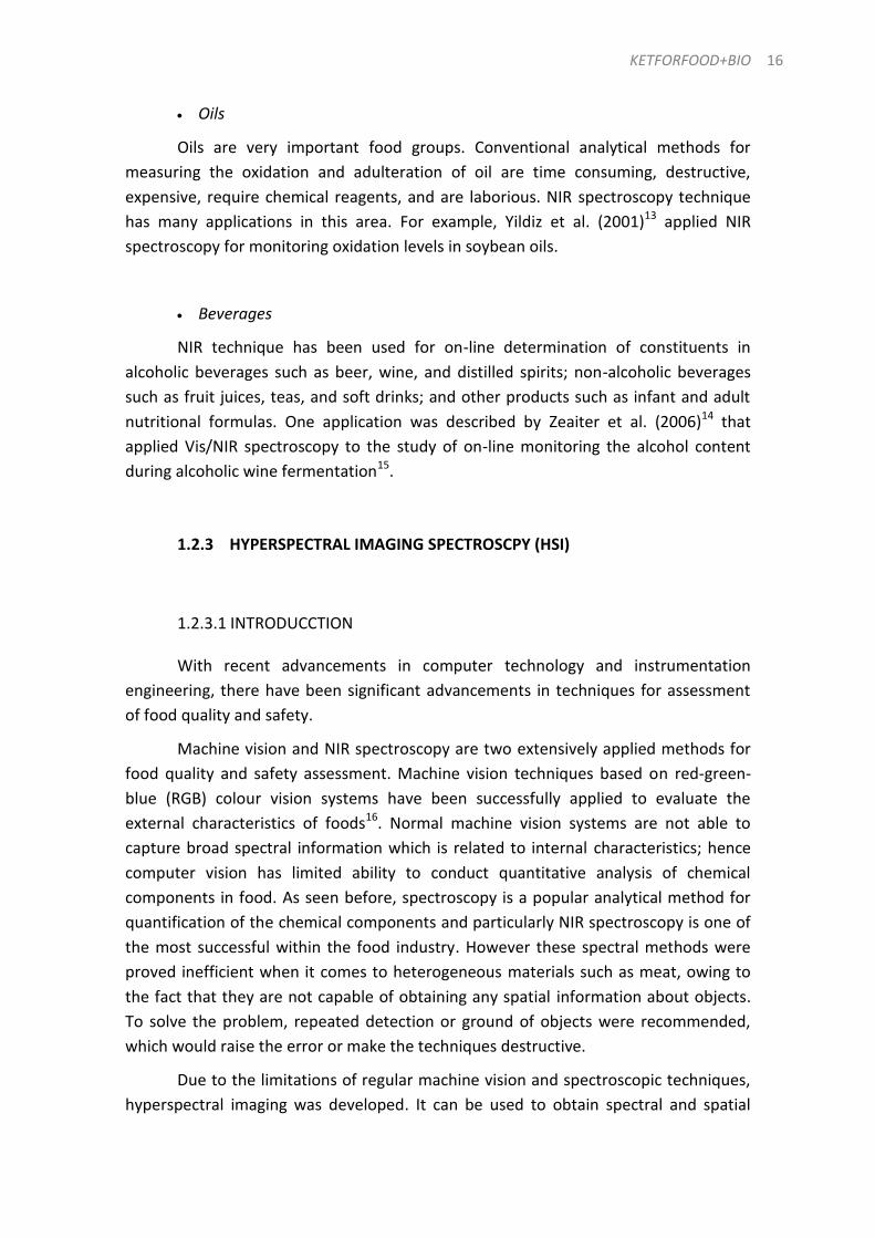
The detector works in line scan mode, ie, the detector senses the spectra of
each pixel line (Figure 3.8). A conveyor was required to pass the samples below the
camera (Figure 3.9). For each sample pixel line a frame was obtained (each frame had
the intensity value for each wavelength) that contain the spectra of all pixels. When all
the frames were join a hypercube was obtained (in that case, the frames were
acquired in video format (.avi).
Figure 3.7. HSI device.
33 NIR techniques and chemometric data analysis applied to food adulteration detection.
To optimize the sampling, the camera was adjusted (height) for the correct data
acquisition. The hamburger diameter was 8 cm, so the appropriate field of view for the
x axis (sample width) (Figure 3.8) of the camera had to be ≃8 cm (Equation 3.1 and
3.2).
3.1
3.2
Once the appropriate height of the camera has been calculated (26,5 cm), the
velocity of the conveyor was calculated to obtain a non-distorted image. For that
purpose, to know the conveyor optimum velocity, the field of view of the y axis was
calculated (Equation 3.3 and 3.4).
3.3
3.4
Figure 3.8. HSI working in line scan mode. Figure 3.9. Conveyor (white ribbon) moving the sample.

KETFORFOOD+BIO 34
The maximum width that the camera could capture in one second depends on
the camera frame rate and was the following one (Equation 3.5):
3.5
Therefore the conveyor velocity was adjusted to that value: ≃18,55 cm/s.
Other parameters that were readjusted in the camera were the Integration time (400
ms) and the number of frames that the camera takes for each sample (500).
The dimensions of the spectral data (hypercube) obtained in each case for
every sample was: 320 x 500 x 256
3.2.2 CONVENTIONAL NIR, METHANOL/ETHANOL EXPERIMENT
The optical system that has been used for sampling was formed by a NIR
detector with a wavelength interval between 880-2348 nm (Stellarnet Red-Wave-NIRx-
S InGaAs-512X; software: SpectraWiz Spectrometer Software v.5.3. de StellarNet Inc.)
(Figure 3.11), a halogen light source (STELLARNET Vis-NIR SL1 Tungsteno-Halógeno
350-2300 nm) (Figure 3.10) and next to it a black compartment to put the sample
inside in a quartz cuvette. An optic fiber transmits the light that passes through the
sample to the detector.
Figure 3.11. Stellarnet Red-Wave-NIRx-S InGaAs-512X.
Figure 3.10. Stellarnet Vis-NIR SL1 Tungsteno-Halógeno 350-2300 nm with a compartment to put the sample.

35 NIR techniques and chemometric data analysis applied to food adulteration detection.
Initial tests allows us to know the optimum operational parameters, that were;
2 ms of detector integration time and a minimum of 50 spectra needed to be averaged
for every sampling. The 2 ms of integration time gave a bright signal of approximately
the 90% of the intensity units dynamic range.
3.2.3 HANDHELD NIR, YOGURT EXPERIMENT
Yogurt samples were taken by a handheld device powered by IRIS (Figure 3.12)
with the following specs (Table 3.7).
Table 3.7. NIR Handheld device specifications
Technical Specs
Sensor InGaAs Espectral range 900-1700 nm Resolution 1 -12 nm
Screen Touch screen 480 x 272 px/ LCD 4,3''
Bits 14 bit Velocity < 2 s
Illumination Halogen lamp 12 V Electric power 230 V (dock station) Data storing Micro SD X 86 B Nano Flash Dimensions 350 x 300 x 120 mm Calibration system Bright and dark references Weight 2,45 Kg Lens mount Standard C mount Temperature 5ºC - +40ºC Data output Ethernet
Core A7 Dual-Core ARM CORTEX 1GB/2GB DDR3 480 MHz
Autonomy > 9 h, dependeing on the use
The advantage of this portable instrument is that is a handy device that permits
working anywhere.
Some parameters were adjusted for the correct data acquisition. The gain by
default was 1, the interval integration time was adjusted to 9 ms and the number of
spectra averaged to take one same was adjusted to 10.
Figure 3.12. Handheld device powered by IRIS.

KETFORFOOD+BIO 36
3.3 SAMPLING
3.3.1 BEEF/COLT EXPERIMENT
Before the sampling procedure the lights were switched and the lid was putted
on the camera shutter to record the dark reference, then, with the lights switched on a
reference white plate (bright reference) was placed above a black support and a video
was recorded by passing the bright below the camera.. This procedure was carried out
every 2 samples, ie, two samples share the same bright/dark references.
All the hamburgers were removed from the refrigeration progressively, with
the same order in which they went introduced. The sampling procedure used was the
following one:
Take the dark reference (If it is required)
Take the bright reference (if it is required)
Take the sample (n), side A (Figure 3.13)
Take the sample (n), side B
Repeat the last two points in order to have a duplicate.
As seen in the procedure, for each hamburger (level of adulteration), two
captures of the up (A) and down (B) side were taken. All the hypercubes (data)
obtained were saved in an external memory for the posterior analysis.
Figure 3.13. Sample passing below the HSI camera for sampling.

37 NIR techniques and chemometric data analysis applied to food adulteration detection.
3.3.2 METHANOL/ETHANOL EXPERIMENT
Every sample, before being read were homogenised manually during 10
seconds. After that the procedure used to take measurements was the following one:
Take the dark reference (light source switched off).
Take the bright reference (plastic cuvette inside the black compartment with
the light source switched on)
Fill the cuvette with the sample and take a measure
Save the data
All samples were analysed under the same conditions trying to minimize
external errors, non-specific to the nature of samples. The analysis was done quickly,
preventing the evaporation of alcohols.
3.3.3 YOGURT EXPERIMENT
Before the 12 hours of refrigeration the sampling started. As in the meat
previous experiment, it was necessary to take bright and a dark references. I that case,
as the samples were not drawn from inside the plastic petri dish the effect of the petri
had to be corrected in the bright sampling. Therefore, a plastic sheet was placed
between the detector and the bright reference.
The user interface of the device is very ‘friendly’, because in each moment
appears in the screen the next step in the sampling procedure. That was the following
one:
Take the dark reference
Take the bright reference
Take the sample (10 replicates per sample)
Finally, the device was connected to a switch which had access to Ethernet
network to send all the data collected to the computer for their analysis.

KETFORFOOD+BIO 38
4. DATA TREATMENT
4.1 DATA STRUCTURE
4.1.1 INTRODUCCTION
All raw data obtained with those equipments are in intensity units, it is
interesting transform this values to absorbance units with the Lambert-Beer law
(Equation 4.1) because exists a lineal relationship between absorbance and the
concentration of the sample, they are proportional.
4.1
Apart from transform the data to absorbance units, to analyse data with
chemometric procedures as PCA or PLS is required to have this dataset as a two
dimensional matrix, normally called calibration matrix
4.1.2 HSI DATA
As explained before, the HSI camera takes the hypercube as a video (.avi), so
the first step was to transform the video to an absorbance hypercube., this procedure
was performed with an Octave routine (Annex 1) using equation 4.1 and taking into
account the bright and dark references.

39 NIR techniques and chemometric data analysis applied to food adulteration detection.
Hypercube, is a tri-dimensional matrix (x,y are the spatial dimensions and λ
represents the wavelength) (Figure 4.1). Every different combination of x and y equals
to one pixel, and each pixel has its own spectrum. It is necessary to transform the
hypercube to a two dimensional matrix to be able to continue with the further
analysis, so the hypercube was restructured to a hypercube matrix (m= rows, number
of pixels and n= columns, number of variables, in that case each pixel spectrum). The
next step was to average this entire two-dimensional hypercube matrix to only get one
spectrum per sample. This procedure was repeated with all samples.
Finally a concatenation of all this averaged spectra was done in order to obtain
the definitive matrix called calibration matrix (m= samples, λ= sample spectra) (Figure
4.2).
Figure 4.1. Transformation of hypercube to an average of the hypercube matrix (two dimensions matrix).
Figure 4.2. Resulting calibration matrix (X) from the average of
the different hypercube samples20
.
KETFORFOOD+BIO 40
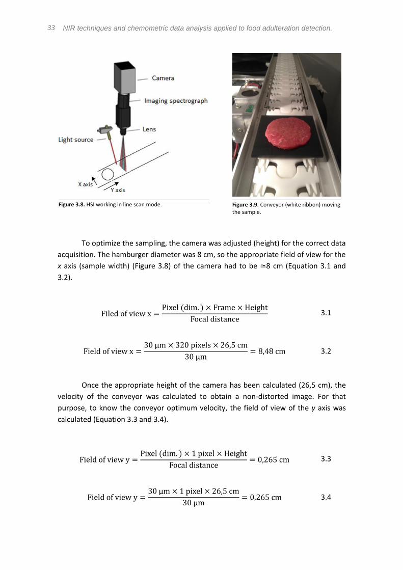
4.1.3 NIR DATA (CONVENTIONAL + HANDHELD)
As in HSI, in both, conventional NIR and handheld device the first thing that was
done was to transform spectra of all samples in absorbance units, to carry out this
action, an Octave routine has been used (Annex 2). With the same software, all data
were concatenated together forming a matrix called calibration matrix (m rows =
number of samples n = number of variables columns in this case is the spectrum of
each of the samples) (Figure 4.3).
4.2 PARTIAL LEAST SQUARES REGRESSION (PLS)
Partial Least Squares Regression is possibly the most widely used method for
multivariate calibration when there is a linear relation between matrix X and matrix Y.
It can be used when there are interferences present in the samples, when the
data have a lot of experimental error, or when the sensors are less selective, for
example. This method is based on the principle that modelling the X matrix is as
important as taking into account the Y matrix, that is, PLS assumes that there are
errors in both blocks and that they have the same importance. Hence, the PLS
components (which are called latent variables) are chosen to maximize the covariance
between X and Y9
The PLS algorithm decomposes the matrices X and Y into scores (T and U) and
loadings (PT and QT) as is shown in equations 4.2 and 4.3 where E and E’ are the error
matrices of X and Y, respectively.
Figure 4.3. Calibration matrix (m= different samples, λ= samples spectra).

41 NIR techniques and chemometric data analysis applied to food adulteration detection.
4.2
4.3
After that, the regression model can be built following equation 4.3 where
is the vector of regression coefficients.
4.3
Usually, cross-validation is used when building the models to determine the
optimal number of components. If the training set is composed by a number of
samples that is small enough, leave-one-out cross-validation can be used and it builds
different models to predict each one of the samples. If the dataset is bigger, it is
divided in segments that include prediction of several samples at the same time
(venetian blinds cross-validation is the one used in this study, for example). It is
important to choose the correct number of latent variables because if a higher number
than necessary is selected, the model is over-fitting the data, which can be dangerous
as it is including noise and other data variation in the calibration. On the other hand, if
the number of chosen components is lower than it should, the model does not use
enough data to correctly predict the necessary parameters.
To validate the calibration model, a set of prediction data is used (it is formed
by data not included in the calibration, if possible): first, the scores are calculated for
the new X matrix (Equation 4.4) and Y vector (Equation 4.5). Afterwards, a new Y
vector is calculated from those scores (Equation 4.6). If the real Y vector is known, it
can be compared to the values obtained through the prediction step, calculating the
error of the model in the prediction.
4.4
4.5
4.6

KETFORFOOD+BIO 42
In the case of hyperspectral imaging detectors, PLS model could make
predictions in two different ways, predict the samples average concentration (as
conventional detectors, explained before) and predict the concentration of each pixel
(image prediction). The image prediction is an additional feature of hyperspectral
imaging detectors, assigning to each pixel a concentration and therefore the spatial
distribution of the components of the sample could be seen.
The variables used to determine whether the model is adequate or not (figures
of merit) are the root mean square errors of calibration, cross-validation and
prediction (RMSEC, RMSECV and RMSEP) shown in equation 4.7 and equation 4.8, the
R2 of the linear regression, and their bias (Equation 4.9).where is the actual
concentration in the sample, is the predicted concentration in the sample (in the
calibration, cross-validation or prediction step) and is the number of samples used in
the dataset.
4.7
4.8
4.9
The R2 is a measure of the lineal relationship between two variables. When R2 is
equal to 1, the variables have a perfect correlation. However, if R2 is 0 means that the
variables do not have any relationship and it is impossible to predict one of them from
the other.
The calibration error (RMSEC), the cross validation error (RMSECV) and the
prediction error (RMSEP) (Equation 4.7 and 4.8) should be as little as possible and have
similar values between them.
The Bias is related with the data systematic error. If the Bias is positive that
means that the prediction will be always higher than the real value of the variable and
if it negative on the contrary. The ideal situation is a Bias value close to 0.

43 NIR techniques and chemometric data analysis applied to food adulteration detection.
5. RESULTS
5.1 DATA PREPROCESSING
After the correct elaboration of the calibration matrix (matrix X), the PLS model
could be generated. The model will relate the samples spectra with the concentration
(matrix Y) (Figure 5.1).
Almost always the dataset require a preprocessing step before the model
generation, aimed to delete abnormal sources of variation. Now are going to be
explained the steps that has been followed for the data preprocessing in each case
until to get the definitive dataset which will be used for the model elaboration.
From this moment, the preprocessing steps, the model creation and the further
validation were done with the SOLO software from Eigenvector Research, Inc.
Figure 5.1. Matrix X: spectra of all samples (m1, m2, mn). Matrix Y: Product concentration of each sample.

KETFORFOOD+BIO 44
5.1.1 BEEF/COLT EXPERIMENT DATA PREPROCESING
The dimensions of the initial calibration matrix (matrix X and matrix Y) for the
meat experiment were:
Matrix X: 84x256 (84 samples per 256 variables)
Matrix Y 84x1 (84 samples concentration values)
The initial spectra of those samples collected in the matrix X was the following
one (Figure 5.2). The Y axis corresponds to absorbance units and the X axis
corresponds to variables, in that case, different wavelengths.
A preliminary wavelength range selection was performed to select less noise
sections. Systematically the wavelength extreme values were delete it.
Different data pre-processings were performed in order to reduce and correct
interferences such as overlapped bands, baseline drifts, scattering, and wavelength
variation. For each pre-processing tested, the model quality parameters obtained were
analysed and the pre-processing that generated the better combination of the
minimum RMSECV, higher R2, lower difference between RMSEC and RMSECV bias close
to zero and optimized numbers of latent factors was selected.
Figure 5.2. Different Colt/Beef spectra of all samples analyzed corresponding to different meat concentrations.

45 NIR techniques and chemometric data analysis applied to food adulteration detection.
As shown in table 5.1 the data pre-processing selected for the PLS model
generation was SNV (rows direction).with 10 LV Therefore, the SNV transformation
proved to be an effective correction, able to remove spectra offsets and slopes caused
by the light scattering intrinsic to solid samples (Figure 5.3).
Table 5.1. Preliminary model quality parameters
Preprocessing Columns Rows LV RMSECV RMSEC CV Bias R2
- SNV 10 5,462 3,714 -0,223 0,962
The regression graph (initial calibration model) related with the quality
parameters shown before are the following one (Figure 5.4). Some anomalous or
extreme values are excluded respect the amount dataset.
Figure 5.3. On the left side the original dataset and on the left side the preprocessed dataset with SNV.

KETFORFOOD+BIO 46
So, the dimensions of the calibration matrix (matrix X and matrix Y) after the
preprocessing steps and the exclusion of anomalous or extreme data for the meat
experiment were:
Matrix X: 50x236 (50 samples per 236 variables)
Matrix Y 50x1 (50 samples concentration values)
These matrixes were the ones that were used for the further model
validation/prediction (validation section).
5.1.2 METHANOL/ETHANOL EXPERIMENT DATA PREPROCESSING
The dimensions of the initial calibration matrix (matrix X and matrix Y) for the
methanol/ethanol experiment were:
Matrix X: 32x490 (32 samples per 490 variables)
Matrix Y 32x1 (32 samples concentration values)
Figure 5.4. Meat initial calibration model. Y measured vs Y predicted.

47 NIR techniques and chemometric data analysis applied to food adulteration detection.
In that case the initial spectra of those samples collected in the matrix X are
composed by 490 variables instead of the 256 variables from the meat experiment due
to the major range wavelength that Stellarnet provides, and was the following one
(Figure 5.5):
A preliminary wavelength range selection was performed to select less noise sections.
Systematically the wavelength extreme values were delete it.
The spectra presents two different clearly parts, the first part from 0 to 160
variables and a second part that goes from 160 to 490 variables. The calibration model
was developed with the entire spectrum as well as only with the different two parts.
The results in all cases are quite similar, but the integration of the second part in the
model requires the use of more latent variables, so only the first part was used.
Different data pre-processings were performed in order to reduce and correct
interferences.
As shown in table 5.2 the data pre-processing selected for the calibration model
generation was a first Derivative with 4 LV Therefore, the first Derivative
transformation proved to be an effective correction, able to remove spectra offsets
and slopes caused by the light scattering intrinsic to liquid samples (Figure 5.6).
Figure 5.5. Different methanol/ethanol spectra of all samples analyzed corresponding to different alcohol concentrations.

KETFORFOOD+BIO 48
Table 5.2. Preliminary model quality parameters
Preprocessing Columns Rows LV RMSECV RMSEC CV Bias R2
- Derivative 4 0,578 0,484 -0,052 0,997
Four latent variables was the value with the minimum RMSECV error (Figure
5.7). This 4 LV explains the 100% of the regression model variance.
Figure 5.6. On the left side the original dataset and on the left side the preprocessed dataset with a first derivative.
Figure 5.7. RMSECV related with LV. Four LV corresponds to the minimum error.

49 NIR techniques and chemometric data analysis applied to food adulteration detection.
The regression graph (initial calibration model) related with the quality
parameters shown before are the following one (Figure 5.8). Some anomalous or
extreme values are excluded respect the amount dataset.
So, the dimensions of the calibration matrix (matrix X and matrix Y) after the
preprocessing steps and the exclusion of one anomalous value for the
methanol/ethanol experiment were:
Matrix X: 31x151 (31 samples per 151 variables)
Matrix Y 31x1 (31 samples concentration values)
These matrixes were the ones that were used for the further model
validation/prediction (validation section).
5.1.3 YOGURT EXPERIMENT DATA PREPROCESSING
The dimensions of the initial calibration matrix (matrix X and matrix Y) for the
yogurt experiment were:
Figure 5.8. Methanol/Ethanol initial calibration model. Y measured vs Y predicted.

KETFORFOOD+BIO 50
Matrix X: 165x256 (165 samples per 256 variables)
Matrix Y 165x1 (165 samples concentration values)
The initial spectra of those samples collected in the matrix X was the following
one (Figure 5.9). The Y axis corresponds to absorbance units and the X axis
corresponds to variables, in that case, different wavelengths.
The Handheld device presents the variables backwards, ie, the variable number
0 corresponds to a wavelength of 1700 nm and the variable 256 coresponds to a
wavelength of 900 nm.
Different data pre-processings were performed in order to reduce and correct
interferences such as overlapped bands, baseline drifts, scattering, and wavelength
variation. For each pre-processing tested, the model quality parameters obtained were
analysed and the pre-processing that generated the better combination of the
minimum RMSECV, higher R2, lower difference between RMSEC and RMSECV bias close
to zero and optimized numbers of latent factors was selected.
As shown in Table 5.3 the data pre-processing selected for the PLS model
generation was Autoscale (columns direction).with 7 LV Therefore, the Autoscale
transformation proved to be an effective correction, able to remove spectra offsets
and slopes caused by the light scattering intrinsic to solid samples (Figure 5.10).
Figure 5.9. Different yogurt spectra of all samples analyzed corresponding to different yogurt fat content.

51 NIR techniques and chemometric data analysis applied to food adulteration detection.
Table 5.3. Preliminary model quality parameters
Preprocessing Columns Rows LV RMSECV RMSEC CV Bias R2
Autoscale - 6 0,443 0,409 -0,0043 0,971
The regression graph (initial calibration model) related with the quality
parameters shown before are the following one (Figure 5.11). Some anomalous or
extreme values are excluded respect the amount dataset.
Figure 5.10. On the left side the original dataset and on the left side the preprocessed dataset with an autoscale.
Figure 5.11. Fat content in yogurt inital model. Y measured vs Y predicted.

KETFORFOOD+BIO 52
So, the dimensions of the calibration matrix (matrix X and matrix Y) after the
preprocessing steps and the exclusion of anomalous or extreme data for the yogurt
experiment were:
Matrix X: 153x256 (153 samples per 256 variables)
Matrix Y 153x1 (153 samples concentration values)
These matrixes were the ones that were used for the further model
validation/prediction (validation section).
5.2 MODELS EXTERNAL VALIDATION
After preprocessing the samples, optimization of variables set (in this case
wavelengths) and exclusion of abnormal samples that did not fit well a PLS calibration
model was generated in each case.
Models are approximate imitations of real-world systems and they never
exactly imitate the real-world system. Due to that, a model should be verified and
validated to the degree needed for the models intended purpose or application.
To perform the model validation, both in meat and yogurt experiment, 1/3 of
the dataset used for the model calibration was removed aimed to be introduced as an
external set of samples to see the ability of the generated model to predict external
samples.
In the methanol/ethanol experiment the model validation were done with a
real external set of samples. Some extra samples were analyzed with the conventional
NIR and then were introduced as new dataset to the calibration matrix.
5.2.1 BEEF/COLT EXPERIMENT VALIDATION
As it has been mentioned before, to perform the meat experiment model
validation, 1/3 of the matrix dataset was removed randomly to see the model
predictive ability.
The dimension of the definitive calibration matrix elaborated in the
preprocessing step was 50 x 236, and after the removal of 1/3 of that dataset the

53 NIR techniques and chemometric data analysis applied to food adulteration detection.
matrix dimension was 33 x 236 (Figure 5.12), so 17 values were predicted in the
validation step.
The quality parameters of the new calibration matrix (33 x 236) were a little bit
modified due the removal of the 17 samples for the validation. The new quality
parameters are summarized in the next table (Table 5.4).
Table 5.4. Calibration matrix quality parameters
LV RMSECV RMSEC CV Bias R2
9 6,832 3,903 -1,60E-01 0,942
At this point was important to take a look to the Variable Importance in
Projection (VIP) scores (Figure 5.13). That tool estimate the importance of each
variable in the projection used in a PLS model and is often used for variable selection.
A variable with a VIP Score close to or greater than 1 (one) can be considered
important in given model. Variables with VIP scores significantly less than 1 (one) are
less important and might be good candidates for exclusion from the model.
Figure 5.12. Meat calibration matrix after remove 1/3 af the dataset for the further validation.

KETFORFOOD+BIO 54
Vip’s graph shows that variables between 50 -75 and 150 -240 are important
for the model estimation, but in that case, a variable selection did not seem to improve
PLS results.
The next step was to upload the 17 previously removed samples to the
calibration matrix and see the ability of the model to predict these values. In the next
graph (Figure 5.14) is seen how the ‘predicted values’, in red, are distributed along the
calibration matrix (grey points).
Figure 5.13. VIP’s scores graph showing the importance of each variable for the model elaboration. Variables above one are important.
Figure 5.14. Prediction results of the meat experiment. In grey, calibration dataset and in red the validation predicted values

55 NIR techniques and chemometric data analysis applied to food adulteration detection.
Table 5.5 presents this prediction in numerical terms, showing the values of the
Y measured (real concentration), Y predicted (predicted concentration), Y residual
(difference between real and predicted concentration) and Y error (standard error) of
each sample that has been used for the validation procedure. The maximum Y residual
(abs) was 7,91.
Table 5.5. Validation predicted values vs measured values, meat experiment
Sample Y Measured Y Predicted Y Residual (abs) Y Error Est
1 94,98 91,1 3,88 7,63 2 85 78,57 6,43 7,49
3 74,97 73,22 1,75 7,47 4 69,86 61,95 7,91 7,36 5 65 60,76 4,24 7,66 6 59,95 63,14 3,19 7,52 7 60,04 58,06 1,98 7,36 8 54,99 53,26 1,73 7,26 9 50,01 47,94 2,07 7,39
10 40,06 37,46 2,6 7,21 11 35,01 33,73 1,28 7,22 12 30,11 35,75 5,64 7,72 13 30,06 32,68 2,62 7,19 14 25,04 25,54 0,5 7,35
15 15,09 17,66 2,57 7,52 16 15,34 20,69 5,35 7,43 17 10,16 15,81 5,65 7,11
The prediction model that was obtained, considering a big amount of samples,
and the spectra pre-treated with SNV showed a good results of RMSECV and RMSEC
6,803 and 3,903 respectively a R2 of 0,942 and a RMSEP of 4,413 (Table 5.6).
As far as the NIR spectroscopy is concerned, even if a precise comparison with
previous studies is difficult due to the differences in meat samples, data
pretreatments, data analysis, etc., the results obtained in the present study are in
agreement with those previously published.by Alamprese et al. (2013) that, also in
terms of meat adulteration detection in the NIR region obtain a PLS model with a
RMSECV and RMSEP of 6,4 and 5,79 respectively.
Table 5.6. Prediction quality parameters
LV RMSECV RMSEC RMSEP CV Bias Pred Bias R2
9 6,832 3,903 4,413 -1,60E-01 -0,252 0,942

KETFORFOOD+BIO 56
Precision is defined in 95% of cases as 2xSDPV, so in that case is: ±8,82 %. The
model are able to predict beef/colt concentrations with a precision of ± 8,82 % in an
interval range of values between 0 and 100%.
1.2.1.1 IMAGE PREDICTION
One of the main perks of the HSI technique is that apart from obtain spectral
information it can also obtain spatial information of a sample. Therefore, instead of
performing the external validation with the spectra averages, the model developed
was applied on the hypercube of each hamburger (image prediction). This allows us to
predict the meat concentration in each pixel, which has an associated spectrum so is
possible to see spatial distributions of the different meat species colt and beef.
The images captured included redundant information, such as the supporting
plate and its surrounding background. For this reason an image-processing step was
needed that resulted in an image mask where only meat tissue is included.
Figure 5.15 shows different levels of beef/colt concentration values. The first
hyperspectral image clearly shows a blue colour predominance corresponding to a
high concentration of beef. The small amount of colt meat present in the burger (5%)
is distributed at the edges of the sample, where the red colour is present. The large
amount of pixels of 100% or 0% can be explained by the grade of mincing of the meat,
the distance of the camera and the size of the pixel, so in each pixel is probably only to
have colt or beef meat.
Figure 5.15. Meat image prediction. Image on the left corresponds to a 5% of Colt, the middle image corresponds to a 50% of Colt and the image on the right side corresponds to a 95% of Colt.

57 NIR techniques and chemometric data analysis applied to food adulteration detection.
In the same figure, the second image (in the middle), corresponds to 50% of
colt, a good mixture of the two meat types was observed as there was not
predominance of one colour or another.
The last picture (on the right side) corresponds to a 95% of colt. Clearly red
colour predominance is observed with some presence of beef in the middle of the
hamburger. Consequently, with this image analysis we are able to detect meat
adulteration as well as to study the sample heterogeneity and thus the mixture
procedure effectiveness.
5.2.2 ETHANOL/METHANOL EXPERIMENT VALIDATION
As it has been mentioned before, to perform the methanol/ethanol experiment
model validation, an external set of analysed samples were added to the calibration
matrix to see the model predictive ability.
The dimension of the definitive calibration matrix elaborated in the
preprocessing step was 31 x 151, and after the removal of 1/3 of that dataset the
matrix dimension was 21 x 151 (Figure 5.16).
The quality parameters of the new calibration matrix (21 x 151) were a little bit
modified due the removal of the 10 samples. The new quality parameters are
summarized in the next table (Table 5.7).
Figure 5.16. Methanol/Ethanol calibration matrix after remove 1/3 af the dataset.

KETFORFOOD+BIO 58
Table 5.7. Calibration matrix quality parameters
LV RMSECV RMSEC CV Bias R2
4 0,566 0,496 -4,30E-02 0,997
Vip’s graph (Figure 5.17) shows that variables between 140 to 170 are
important for the model estimation, but in that case, a variable selection did not seem
to improve PLS results
The next step was to add the 10 external set of samples to the calibration
matrix and see the ability of the model to predict these values. In the next graph
(Figure 5.18) is seen how the ‘predicted values’, in red, are distributed along the
calibration matrix (grey points).
Figure 5.17. VIP’s scores graph showing the importance of each variable for the model elaboration. Variables above one are important

59 NIR techniques and chemometric data analysis applied to food adulteration detection.
Table 5.8 presents this prediction in numerical terms, showing the values of the
Y measured (real concentration), Y predicted (predicted concentration), Y residual
(difference between real and predicted concentration) and Y error (standard error) of
each sample that has been used for the validation procedure. The maximum Y residual
(abs) was 0,836.
Table 5.8. Validation predicted values vs measured values, methanol/ethanol experiment.
Sample Y Measur. Y Predic. Y Res. (abs) Y Stdnt Res. Y Error Est.
1 1,75 1,538 0,212 -0,344 0,63
2 2,45 2,129 0,321 -0,519 0,663
3 3,5 3,587 0,087 0,141 0,673
4 10,5 10,565 0,065 0,105 0,686
5 14 14,159 0,159 0,257 0,69
6 19,25 19,205 0,045 -0,073 0,698
7 22,75 22,314 0,436 -0,706 0,655
8 28 27,267 0,733 -1,185 0,654
9 31,5 30,664 0,836 -1,353 0,642
10 33,25 32,578 0,672 -1,087 0,672
In that case the Y Studentized is also shown. Is an indication of the lack of fit of
a sample, is a count of the number of standard deviations, for example the sample
with a value of 0,836 of Y residual has a Y Studentized. of 1,353, that means that the
sample are deviated 1,353 times.
Figure 5.18. Prediction results of ethanol/methanol experiment. In grey, calibration dataset and in red the validation predicted values

KETFORFOOD+BIO 60
The prediction model that was obtained with the spectra pre-treated with a
first derivative showed a very good results of RMSECV and RMSEC 0,566 and 0,496
respectively a R2 of 0,998 and a RMSEP of 0,454 (Table 5.9).
Table 5.9. Prediction quality parameters
LV RMSECV RMSEC RMSEP CV Bias Pred Bias R2
4 0,566 0,496 0,454 -4,30E-02 -0,29 0,998
Precision is defined in 95% of cases as 2xSDPV, so in that case is: ± 0,9%. The
model are able to predict methanol/ethanol different concentrations with a precision
of ± 0,9% in an interval range of values between 0 and 35%, that is equivalent to a
precision of 0,354 g/L
The Spanish law ‘’Ley 25/1970 2 de Diciembre, Estatuto Viña, Vino y alcoholes’’
Allows the presence of methanol with a maximum value in wine of 0,5 g/L and in
natural alcohols of 2 g/L, so the calibration model that has been obtained in that
experiment are able to detect methanol concentrations below the maximum
permitted values in commercial beverages.
The results obtained in the present study are resembled with those previously
published by Dambergs et al. (2002) that working in the NIR region obtained four
calibration models with an R2 of 0,998 and with a RMSEP between 0,06 and 4,55 g/L in
terms of distillates derived from the production of wine-fortifying spirit.
5.2.3 YOGURT EXPERIMENT VALIDATION
As it has been mentioned before, to perform the yogurt experiment model
validation, 1/3 of the matrix dataset was removed randomly to see the model
predictive ability.
The dimension of the definitive calibration matrix elaborated in the
preprocessing step was 153 x 256, and after the removal of 1/3 of that dataset the
matrix dimension was 110 x 256 (Figure 5.19), so 43 values were predicted in the
validation step.

61 NIR techniques and chemometric data analysis applied to food adulteration detection.
The quality parameters of the new calibration matrix (110 x 256) were a little
bit modified due the removal of the 43 samples for the validation. The new quality
parameters are summarized in the next table (Table 5.10).
Table 5.10. Calibration quality parameters
Vip’s graph (Figure 5.20) shows that variables between 125 to 175 are
important for the model estimation, but in that case, a variable selection did not seem
to improve PLS results
LV RMSECV RMSEC CV Bias R2
6 0,443 0,390 0,0014 0,973
Figure 5.19. Yogurt fat detection calibration matrix after remove 1/3 af the dataset for the further validation

KETFORFOOD+BIO 62
The next step was to upload the 43 previously removed samples to the
calibration matrix and see the ability of the model to predict these values. In the next
graph (Figure 5.21) is seen how the ‘predicted values’, in red, are distributed along the
calibration matrix (grey points).
Figure 5.20. VIP’s scores graph showing the importance of each variable for the model elaboration. Variables above one are important
Figure 5.21. Prediction results of yogurt experiment. In grey, calibration dataset and in red the validation predicted values

63 NIR techniques and chemometric data analysis applied to food adulteration detection.
Table 5.11 presents this prediction in numerical terms, showing the values of
the Y measured (real concentration), Y predicted (predicted concentration), Y residual
(difference between real and predicted concentration) and Y error (standard error) of
each sample that has been used for the validation procedure. The maximum Y residual
(abs) was 7,91.
Table 5.11. Validation predicted values vs measured values yogurt experiment.
Sample Y Measured Y Predicted Y Residual (abs) Y Stdnt Res Y Error Est
1 0,710 0,976 0,267 0,641 0,455 2 0,710 1,182 0,472 1,136 0,457 3 0,710 0,059 0,651 -1,565 0,472 4 0,710 0,222 0,487 -1,172 0,454 5 1,419 1,451 0,032 0,077 0,461 6 1,419 1,364 0,055 -0,132 0,460 7 1,419 1,086 0,333 -0,799 0,447 8 1,419 1,292 0,127 -0,306 0,450 9 2,124 2,182 0,058 0,139 0,447
10 2,832 2,680 0,152 -0,365 0,459 11 2,832 2,762 0,070 -0,168 0,453 12 2,832 4,190 1,358 3,263 0,459 13 2,832 3,411 0,579 1,391 0,446 14 3,546 4,537 0,991 2,381 0,454 15 3,546 4,131 0,585 1,407 0,447 16 3,546 4,037 0,491 1,180 0,448 17 4,241 4,233 0,008 -0,020 0,465 18 4,241 4,395 0,153 0,368 0,458 19 4,241 4,281 0,039 0,095 0,446 20 4,241 4,647 0,406 0,975 0,454 21 4,959 4,873 0,086 -0,208 0,453 22 4,959 4,744 0,215 -0,517 0,446 23 4,959 5,202 0,243 0,583 0,458 24 4,959 5,590 0,630 1,515 0,448 25 4,959 4,862 0,097 -0,234 0,446 26 5,666 5,419 0,247 -0,594 0,447 27 5,666 5,436 0,229 -0,552 0,455 28 5,666 5,226 0,439 -1,056 0,485 29 6,376 5,983 0,393 -0,944 0,454 30 6,376 5,973 0,403 -0,968 0,452 31 6,376 6,413 0,037 0,089 0,447 32 6,376 5,634 0,741 -1,782 0,447 33 7,081 7,182 0,100 0,242 0,451 34 7,081 7,306 0,224 0,539 0,451 35 7,081 6,595 0,487 -1,169 0,446 36 7,081 7,281 0,199 0,479 0,449 37 7,792 7,454 0,338 -0,813 0,448

KETFORFOOD+BIO 64
Sample Y Measured Y Predicted Y Residual (abs) Y Stdnt Res Y Error Est
38 7,792 7,267 -0,525 -1,262 0,466 39 7,792 7,397 -0,395 -0,949 0,456 40 7,792 7,674 -0,118 -0,285 0,458 41 8,500 8,924 0,424 1,019 0,464 42 8,500 7,814 -0,686 -1,649 0,452 43 8,500 7,733 -0,767 -1,844 0,454
The prediction model that was obtained with the spectra pre-treated with an
autoscale showed a very good results of RMSECV and RMSEC 0,39 and 0,46
respectively a R2 of 0,975 and a RMSEP of 0,443 (Table 5.12).
Table 5.12. Calibration quality parameters
LV RMSECV RMSEC RMSEP CV Bias Pred Bias R2
6 0,443 0,390 0,460 -0,0014 -0,002 0,975
Precision is defined in 95% of cases as 2xSDPV, so in that case is: ± 0,92% The
model are able to detect and predict different levels of fats in yogurts with a precision
of ± 0,92% in an interval range of values between 0 and 9,9% of fat content.

65 NIR techniques and chemometric data analysis applied to food adulteration detection.
6. CONCLUSIONS
The ability of NIR spectroscopy for the detection and quantification of food
adulteration by various optical systems and/or techniques have been analysed.
The Hyperspectral imaging spectroscopy is adequate for the detection of meat
adulteration with a precision of 8,8% in a range of 0 to 100% using a PLS model with a
R2 of 0,94 and a RMSEP of 4,4. In addition, the HSI image prediction is able to detect
meat adulteration as well as to study the sample heterogeneity and thus the meat
mixture and the procedure elaboration effectiveness.
With regard to the conventional NIR, this equipment is adequate for the
detection of fraudulent addition of methanol in alcoholic beverages with a precision of
0,9% in a range from 0 to 35% using a PLS model with a R2 value of 0,998 and a RMSEP
of 0,45.
The Handheld device is suitable for the detection of fraud in the fat content of
natural yogurts with a precision of 0,92% in a range of 0 to 9,9% using a PLS model
with a R2 of 0,975 and a RMSEP of 0,46.
All in all, NIR techniques seem an attractive solution to detect adulterations in
food industry. Therefore, they could be a substitute or complement to conventional
laborious and time-consuming analytical techniques nowadays employed in the food
quality control.

KETFORFOOD+BIO 66
7. BIBLIOGRAPHY
1. Fernández Pierna, J. a. et al. NIR hyperspectral imaging spectroscopy and
chemometrics for the detection of undesirable substances in food and feed.
Chemom. Intell. Lab. Syst. 117, 233–239 (2012).
2. Vitale, R. et al. A rapid and non-invasive method for authenticating the origin of
pistachio samples by NIR spectroscopy and chemometrics. Chemom. Intell. Lab.
Syst. 121, 90–99 (2013).
3. Ballin, N. Z., Vogensen, F. K. & Karlsson, A. H. Species determination - Can we
detect and quantify meat adulteration? Meat Sci. 83, 165–74 (2009).
4. Liu, Y. et al. Prediction of chemical composition and geographical origin
traceability of Chinese export tilapia fillets products by near infrared
reflectance spectroscopy. LWT - Food Sci. Technol. 60, 1214–1218 (2015).
5. Ropodi, a. I., Pavlidis, D. E., Mohareb, F., Panagou, E. Z. & Nychas, G.-J. E.
Multispectral image analysis approach to detect adulteration of beef and pork
in raw meats. Food Res. Int. 67, 12–18 (2015).
6. Process Analytical Technology for the Food Industry. 3, 301 (Springer, 2014).
7. Ma, J. et al. Application of Vis–NIR hyperspectral imaging in classification
between fresh and frozen-thawed pork Longissimus Dorsi muscles. Int. J. Refrig.
50, 10–18 (2015).
8. Huang, H., Yu, H., Xu, H. & Ying, Y. Near infrared spectroscopy for on/in-line
monitoring of quality in foods and beverages: A review. J. Food Eng. 87, 303–
313 (2008).
9. Francisco, A., González, M. & Valero, E. L. Desarrollo de un método de selección
de variables para datos espectroscópicos en el infrarrojo cercano . Índice.
(2004).

67 NIR techniques and chemometric data analysis applied to food adulteration detection.
10. Huck-Pezzei, V. a. et al. Alps food authentication, typicality and intrinsic quality
by near infrared spectroscopy. Food Res. Int. 62, 984–990 (2014).
11. Kucheryavskiy, S. & Lomborg, C. J. Monitoring of whey quality with NIR
spectroscopy—A feasibility study. Food Chem. 176, 271–277 (2015).
12. Bramble, T., Herrman, T. J., Loughin, T. & Dowell, F. Single Kernel Protein
Variance Structure in Commercial Wheat Fields in Western Kansas. Crop Sci. 42,
1488 (2002).
13. Yildiz, G., Wehling, R. L. & Cuppett, S. L. Method for determining oxidation of
vegetable oils by near-infrared spectroscopy. J. Am. Oil Chem. Soc. 78, 495–502
(2001).
14. Zeaiter, M., Roger, J. M. & Bellon-Maurel, V. Dynamic orthogonal projection. A
new method to maintain the on-line robustness of multivariate calibrations.
Application to NIR-based monitoring of wine fermentations. Chemom. Intell.
Lab. Syst. 80, 227–235 (2006).
15. Wu, D. & Sun, D.-W. Advanced applications of hyperspectral imaging
technology for food quality and safety analysis and assessment: A review —
Part I: Fundamentals. Innov. Food Sci. Emerg. Technol. 19, 1–14 (2013).
16. Erkinbaev, C. et al. Contactless and non-destructive differentiation of
microstructures of sugar foams by hyperspectral scatter imaging. Innov. Food
Sci. Emerg. Technol. 24, 131–137 (2014).
17. Kamruzzaman, M., Makino, Y. & Oshita, S. Non-invasive analytical technology
for the detection of contamination, adulteration, and authenticity of meat,
poultry, and fish: a review. Anal. Chim. Acta 853, 19–29 (2015).
18. Huang, H., Liu, L. & Ngadi, M. O. Recent developments in hyperspectral imaging
for assessment of food quality and safety. Sensors (Basel). 14, 7248–76 (2014).
19. Qin, J., Chao, K., Kim, M. S., Lu, R. & Burks, T. F. Hyperspectral and multispectral
imaging for evaluating food safety and quality. J. Food Eng. 118, 157–171
(2013).
20. Gowen, A. & Imaging, H. Hyperspectral Imaging and Chemometrics : A Perfect
Combination for the Analysis of Food Structure , Composition and Quality. 28,
343–370 (2013).
21. Kamruzzaman, M., Elmasry, G., Sun, D.-W. & Allen, P. Non-destructive
assessment of instrumental and sensory tenderness of lamb meat using NIR
hyperspectral imaging. Food Chem. 141, 389–96 (2013).
22. Ricardo, J. & Gutiérrez, L. Aplicación de Métodos Quimiométricos para la
Caracterización y Control de Calidad de Plantas Medicinales

KETFORFOOD+BIO 68
23. Alamprese, C., Casale, M., Sinelli, N., Lanteri, S. & Casiraghi, E. Detection of
minced beef adulteration with turkey meat by UV–vis, NIR and
MIR spectroscopy. LWT - Food Sci. Technol. 53, 225–232 (2013).
MORE BIBLIOGRAPHY
Xu, L., Shi, W., Cai, C.-B., Zhong, W. & Tu, K. Rapid and nondestructive detection of
multiple adulterants in kudzu starch by near infrared (NIR) spectroscopy and
chemometrics. LWT - Food Sci. Technol. 61, 590–595 (2015).
Xiong, Z., Sun, D.-W., Zeng, X.-A. & Xie, A. Recent developments of hyperspectral
imaging systems and their applications in detecting quality attributes of red
meats: A review. J. Food Eng. 132, 1–13 (2014).
Sentandreu, M. Á. & Sentandreu, E. Authenticity of meat products: Tools against
fraud. Food Res. Int. 60, 19–29 (2014).
Rungpichayapichet, P., Mahayothee, B., Khuwijitjaru, P., Nagle, M. & Müller, J.
Non-destructive determination of β-carotene content in mango by near-
infrared spectroscopy compared with colorimetric measurements. J. Food
Compos. Anal. 38, 32–41 (2015).
Kucheryavskiy, S. & Lomborg, C. J. Monitoring of whey quality with NIR
spectroscopy—A feasibility study. Food Chem. 176, 271–277 (2015).
Dambergs, R. G., Kambouris, A., Francis, I. L. & Gishen, M. Rapid analysis of
methanol in grape-derived distillation products using near-infrared
transmission spectroscopy. J. Agric. Food Chem. 50, 3079–84 (2002).

69 NIR techniques and chemometric data analysis applied to food adulteration detection.
8. TABLE OF FIGURES INTRODUCCTION
EXPERIMENTAL
Figure 3.1. Original beef samples.
Figure 3 2. Minced colt meat (left) and minced beef meat (right).
Figure 3.3. Example of a prepared hamburger.
Figure 3.4. Plastic dish used for the hamburgers elaboration.
Table 3.1. Theoretical meat weights (g) at different beef/colt concentration.
Table 3.2. Real meat weights (g) at different beef/colt concentration. Two hamburgers (A and B) per level.
Table 3.3. Different methanol concentration samples used for the test.
Table 3.4. Initial amount of water and alcohol used for the initial samples preparation.
Figure 3.5. Original Greek yogurt and skimmed yogurt samples,
Table 1.1. Infrared spectrum region division.
Figure 1.1. Table of NIR absorption bands at different wavelengths.
Figure 1.2. Evolution of the number of paper published related with hyperspectral imaging technique in the last 20 years .
Figure 1.3. Schematic diagram of Hyperspectral image, Hypercube acquisition (left). Spectrum of one pixel of the hypercube (right).
Figure 1.4. Different possibilities to obtain a hypercube (x, y, λ). Area scanning, point scanning, line scanning, and single shot.
Figure 1.5. Main components of a push broom hyperspectral imaging system.
Figure 1.6. Typical HSI detector (CCD camera) integrated with a spectrograph as a previous element of wavelength dispersion.
Figure 1.7. Different image sensing modes, Reflectance, Transmittance and Transreflectance.

KETFORFOOD+BIO 70
Figure 3.6. Petri dish with yogurt simple
Table 3.5. Different yogurt samples in duplicate (A and B) used for the test from a concentration from 0 to 9,9 %. Theoretical and real percentages (%) and weights (g).
Table 3.6. Hyperspectral imaging device specifications
Figure 3.7. HSI device
Figure 3.8. HSI working in line scan mode
Figure 3.9. Conveyor (white ribbon) moving the sample
Figure 3.10. Stellarnet Vis-NIR SL1 Tungsteno-Halógeno 350-2300 nm
Figure 3.11. Stellarnet Red-Wave-NIRx-S InGaAs-512X
Table 3.7. NIR Handheld device specifications
Figure 3.12. Handheld device powered by IRIS
Figure 3.13. Sample passing below the HIS camera for sampling.
DATA TREATMENT
Figure 4.1. Transformation of hypercube to an average of the hypercube matrix (two dimensions matrix).
Figure 4.2. Resulting calibration matrix (X) from the average of the different hypercube samples.
Figure 4.3. Calibration matrix (m= different samples, λ= samples spectra
RESULTS
Figure 5.1. Matrix X: spectra of all samples (m1, m2, mn). Matrix Y: Product concentration of each sample
Figure 5.2. Different Colt/Beef spectra of all samples analyzed corresponding to different meat concentrations
Table 5.1. Preliminary model quality parameters
Figure 5.3. On the left side the original dataset and on the left side the preprocessed dataset with SNV.
71 NIR techniques and chemometric data analysis applied to food adulteration detection.
Figure 5.4. Meat initial calibration model. Y measured vs Y predicted.
Figure 5.5. Different methanol/ethanol spectra of all samples analyzed corresponding to different alcohol concentrations.
Table 5.2. Preliminary model quality parameters.
Figure 5.6. On the left side the original dataset and on the left side the preprocessed dataset with a first derivative.
Figure 5.7. RMSECV related with LV. Four LV corresponds to the minimum error.
Figure 5.8. Methanol/Ethanol initial calibration model. Y predicted vs Y measured.
Figure 5.9. Different yogurt spectra of all samples analyzed corresponding to different yogurt fat content.
Table 5.3. Preliminary model quality parameters.
Figure 5.10. On the left side the original dataset and on the left side the preprocessed dataset with an autoscale.
Figure 5.11. Yogurt fat content initial calibration model. Y predicted vs Y measured.
Figure 5.12. Meat calibration matrix after remove 1/3 af the dataset for the further validation.
Table 5.4. Calibration matrix quality parameters.
Figure 5.13. VIP’s scores graph showing the importance of each variable for the model elaboration.
Figure 5.14. Prediction results of the meat experiment. In grey, calibration dataset and in red the validation predicted values.
Table 5.5. Validation predicted values vs measured values, meat experiment.
Table 5.6. Prediction quality parameters.
Figure 5.15. Meat image prediction. Image on the left corresponds to a 5% of Colt, the middle image corresponds to a 50% of Colt and the image on the right side corresponds to a 95% of Colt.
Figure 5.16. Methanol/Ethanol calibration matrix after remove 1/3 of the dataset.
Table 5.7. Calibration matrix quality parameters.
Figure 5.17. VIP’s scores graph showing the importance of each variable for the model elaboration.

KETFORFOOD+BIO 72
Figure 5.18. Prediction results of ethanol/methanol experiment. In grey, calibration dataset and in red the validation predicted values.
Table 5.8. Validation predicted values vs measured values, methanol/ethanol experiment.
Table 5.9. Prediction quality parameters.
Figure 5.19. Yogurt fat detection calibration matrix after remove 1/3 of the dataset for the further validation.
Table 5.10. Calibration quality parameters.
Figure 5.20. VIP’s scores graph showing the importance of each variable for the model elaboration. Variables above one are important.
Figure 5.21. Prediction results of yogurt experiment. In grey, calibration dataset and in red the validation predicted values.
Table 5.11. Validation predicted values vs measured values, methanol/ethanol experiment.
Table 5.12 Calibration quality parameters.

73 NIR techniques and chemometric data analysis applied to food adulteration detection.
9. ABREVIATURES
3D: Three dimensions
CI: Chemical imaging
CV: Cross validation
FIR: Far infrared
HSI: Hyperspectral imaging
LV: Latent variable
MID: Mid infrared
NIR: Near infrared
PAT: Process analytical technology
PC: Principal component
PCA: Principal component analysis
PLS: Partial least squares
RMSEC: Root mean square error of calibration
RMSCV: Root mean square error of cross validation
RMSEP: Root mean square error of prediction
VIP: Variable importance in PLS projections

KETFORFOOD+BIO 74
10. ANNEXES
ANNEX 1: VIDEO TO HYPERCUBE, HSI
Function
abs_hyp_todos_prueba(nbright,ndark,ni,nf,filename)
;
%Bright hypercube construction
namel=strcat('mplayer.exe -vo
png',"\t",'bright',num2str(nbright),'.avi');
system(namel);
listofpng=dir('*.png');
numofpng=numel(listofpng);
for i=1:numofpng;
if i<10;
string=strcat('0000000',num2str(i));
elseif i<100;
string=strcat('000000',num2str(i));
else;
string=strcat('00000',num2str(i));
end;
A=imread([string '.png']);
if i==1;
J=A;
else;
J=cat(3,J,A);
end;
end;
P=permute(J,[2 3 1]);
clear J;
clear A;
clear string;
clear listofpng;
clear namel;
clear numofpng;
%Dark hypercube construction
namel=strcat('mplayer.exe -vo
png',"\t",'dark',num2str(ndark),'.avi');
system(namel);
listofpng=dir('*.png');
numofpng=numel(listofpng);
for i=1:numofpng;
if i<10;
string=strcat('0000000',num2str(i));
elseif i<100;
string=strcat('000000',num2str(i));
else;
string=strcat('00000',num2str(i));
end;
A=imread([string '.png']);
if i==1;
J=A;
else;
J=cat(3,J,A);
end;
end;
B=permute(J,[2 3 1]);
clear J;
clear A;
clear string;
clear listofpng;
clear namel;
clear numofpng;
for i=ni:nf;
%Sample hypercube (up)
namel=strcat('mplayer.exe -vo
png',"\t",'spect',num2str(i),'_up.avi');
system(namel);
listofpng=dir('*.png');
numofpng=numel(listofpng);
for j=1:numofpng;
if j<10;
string=strcat('0000000',num2str(j));
elseif j<100;

75 NIR techniques and chemometric data analysis applied to food adulteration detection.
string=strcat('000000',num2str(j));
else;
string=strcat('00000',num2str(j));
end;
A=imread([string '.png']);
if j==1;
J=A;
else;
J=cat(3,J,A);
end;
end;
C=permute(J,[2 3 1]);
clear J;
clear A;
clear string;
clear listofpng;
clear namel;
clear numofpng;
%Absorbace sample hypercube(up)
rest1=single(C)-single(B);
clear C;
rest1(rest1<0)=0;
rest2=single(P)-single(B);
rest2(rest2<0)=0;
div=(rest1)./(rest2);
clear rest1;
clear rest2;
div(~isfinite(div))=1;
div(isnan(div))=1;
div(div==0)=0.1;
abs=log10(1./div);
clear div;
filenamel=[filename num2str(i) '_up','.mat'];
save ('-mat',filenamel,'abs');
clear abs;
%Sample hypercube (down)
namel=strcat('mplayer.exe -vo
png',"\t",'spect',num2str(i),'_down.avi');
system(namel);
listofpng=dir('*.png');
numofpng=numel(listofpng);
for j=1:numofpng;
if j<10;
string=strcat('0000000',num2str(j));
elseif j<100;
string=strcat('000000',num2str(j));
else;
string=strcat('00000',num2str(j));
end;
A=imread([string '.png']);
if j==1;
J=A;
else;
J=cat(3,J,A);
end;
end;
C=permute(J,[2 3 1]);
clear J;
clear A;
clear string;
clear listofpng;
clear namel;
clear numofpng;
%Sample hypercube DEF.
rest1=single(C)-single(B);
clear C;
rest1(rest1<0)=0;
rest2=single(P)-single(B);
rest2(rest2<0)=0;
div=(rest1)./(rest2);
clear rest1;
clear rest2;
div(~isfinite(div))=1;
div(isnan(div))=1;
div(div==0)=0.1;
abs=log10(1./div);
clear div;
filenamel=[filename num2str(i) '_down','.mat'];
save ('-mat',filenamel,'abs');
clear abs;
end;
clear P;
clear B;
ANNEX 2: TRANSFORMATION,
INTESITY TO ABSORBANCE, NIR
function
m=Abs_total(ni,nf,name,extension,namebright,nbrig
ht,name_Abstotal);
i=nbright;
filenamel=[namebright num2str(i) extension];
B=dlmread(filenamel,'',2,0);
B=B(:,2);
B=B';
B(B<0)=0;

KETFORFOOD+BIO 76
for i=ni:nf;
filename=[name num2str(i) extension];
A=dlmread (filename,'',2,0);
A=A(:,2);
A=A';
A(A<0)=0;
div=A./B;
div(~isfinite(div))=1;
div(isnan(div))=1;
div(div==0))=0.1;
Abs=log10(1./div);
name_Abstotal=cat(1,name_Abstotal,Abs);
end;
m=name_Abstotal;

77 NIR techniques and chemometric data analysis applied to food adulteration detection.