NIPRL Chapter 1. Probability Theory 1.1 Probabilities 1.2 Events 1.3 Combinations of Events 1.4...
57
NIPRL Chapter 1. Probability Theory 1.1 Probabilities 1.2 Events 1.3 Combinations of Events 1.4 Conditional Probability 1.5 Probabilities of Event Intersections 1.6 Posterior Probabilities
-
Upload
silas-donald-davidson -
Category
Documents
-
view
229 -
download
0
Transcript of NIPRL Chapter 1. Probability Theory 1.1 Probabilities 1.2 Events 1.3 Combinations of Events 1.4...

NIPRL
Chapter 1. Probability Theory
1.1 Probabilities1.2 Events1.3 Combinations of Events1.4 Conditional Probability1.5 Probabilities of Event Intersections1.6 Posterior Probabilities

NIPRL
CHAPTER 1 Probability Theory1.1 Probabilities1.1.1 Introduction
• Statistics and Probability theory constitutes a branch of mathematics for dealing with uncertainty
• Probability theory provides a basis for the science of statistical inference from data

NIPRL
CHAPTER 1 Probability Theory1.1 Probabilities1.1.2 Sample Spaces(1/3)
• Experiment : any process or procedure for which more than one outcome is possible
• Sample Space The sample space S of an experiment is a set consisting of
all of the possible experimental outcomes.

NIPRL
1.1.2 Sample Spaces(2/3)
• Example 3: Software Errors The number of separate errors in a particular piece of
software can be viewed as having a sample space
• Example 4: Power Plant Operation A manager supervises the operation of three power plants,
at any given time, each of the three plants can be classified as either generating electricity (1) or being idle (0).
{0 errors, 1errors, 2errors, 3errors,...}S
{(0,0,0) (0,0,1) (0,1,0) (0,1,1) (1,0,0) (1,0,1) (1,1,0) (1,1,1)}S

NIPRL
1.1.2 Sample Spaces(3/3)
• GAMES OF CHANCE - Games of chance commonly involve the toss of a coin, the
roll of a die, or the use of a pack of cards. - The roll of a die A usual six-sided die has a sample space
If two dice are rolled ( or, equivalently, if one die is rolled twice), the sample space is shown in Figure 1.2.
{1,2,3,4,5,6}S

NIPRL
1.1.3 Probability Values(1/5)
• Probabilities A set of probability values for an experiment with a
sample space consists of some probabilities
that satisfy
and
The probability of outcome occurring is said to be , and this is written
( )i iP O p
ipiO1 2 1np p p
1 20 1,0 1, ,0 1np p p
1 2, , , np p p1 2{ , , , }nS O O O

NIPRL
1.1.3 Probability Values(2/5)
• Example 3 Software Errors Suppose that the numbers of errors in a software product
have probabilities
There are at most 5 errors since the probability values are zero for 6 or more errors.
The most likely number of errors is 2. 3 and 4 errors are equally likely in the software product.
(0 errors) 0.05, (1 error) 0.08, (2 errors) 0.35,
(3errors) 0.20, (4 errors) 0.20, (5 errors) 0.12,
( errors) 0, for 6
P P P
P P P
P i i

NIPRL
1.1.3 Probability Values(3/5)
• In some situations, notably games of chance, the experiments are conducted in such a way that all of the possible outcomes can be considered to be equally likely, so that they must be assigned identical probability values.
• n outcomes in the sample space that are equally likely => each probability value be 1/n.
NIPRL
1.1.3 Probability Values(4/5)
• GAMES OF CHANCE - A fair die will have each of the six outcomes equally likely. - An example of a biased die would be one of which
In this case the die is most likely to score a 6, which will happen roughly three times out of ten as a long-run
average.
1(1) (2) (3) (4) (5) (6)
6P P P P P P

NIPRL
1.1.3 Probability Values(5/5) - If two die are thrown and each of the 36 outcomes is
equally likely ( as will be the case two fair dice that are shaken properly), the probability value of each outcome will necessarily be 1/36

NIPRL
1.2 Events1.2.1 Events and Complements(1/6)
• Events An event A is a subset of the sample space S. It collects
outcomes of particular interest. The probability of an event is obtained by summing the probabilities of the
outcomes contained within the event A.
• An event is said to occur if one of the outcomes contained within the event occurs.
, ( ),A P A

NIPRL
1.2.1 Events and Complements(2/6)
• A sample space consists of eight outcomes with a probability value.
S
'
( ) 0.10 0.15 0.30 0.55
( ) 0.10 0.05 0.05 0.15 0.10 0.45
Notice that ( ) ( ) 1.
P A
P A
P A P A

NIPRL
1.2.1 Events and Complements(3/6)
• Complements of Events The event , the complement of event A, is the event
consisting of everything in the sample space S that is not contained within the event A. In all cases
• Events that consist of an individual outcome are sometimes referred to as elementary events or simple events
A
( ) ( ) 1P A P A

NIPRL
1.2.1 Events and Complements(4/6)
• Example 3 Software Errors Consider the event A that there are no more than two
errors in a software product. A = { 0 errors, 1 error, 2 errors } S and P(A) = P(0 errors) + P(1 error) + P(2 errors) = 0.05 + 0.08 + 0.35 = 0.48
P( ) = 1 – P(A) = 1 – 0.48 = 0.52
A

NIPRL
1.2.1 Events and Complements(5/6)• GAMES OF CHANCE - even = { an even score is recorded on the roll of a die } = { 2,4,6 } For a fair die, - A = { the sum of the scores of two dice is equal to 6 } = { (1,5), (2,4), (3,3), (4,2), (5,1) }
A sum of 6 will be obtained with two fair dice roughly 5 times out of 36 on average, that is, on about 14% of the throws.
1 1 1 1(even) (2) (4) (6)
6 6 6 2P P P P
1 1 1 1 1 5( )
36 36 36 36 36 36P A

NIPRL
1.2.1 Events and Complements(6/6)
- B = { at least one of the two dice records a 6 }
11( )
3611 25
( ) 136 36
P B
P B

NIPRL
1.3 Combinations of Events1.3.1 Intersections of Events(1/5)
• Intersections of Events The event is the intersection of the events A and B
and consists of the outcomes that are contained within both events A and B. The probability of this event, , is the probability that both events A and B occur simultaneously.
A B
( )P A B

NIPRL
1.3.1 Intersections of Events(2/5)
• A sample space consists of 9 outcomesS
( ) 0.01 0.07 0.19 0.27
( ) 0.07 0.19 0.04 0.14 0.12 0.56
( ) 0.07 0.19 0.26
P A
P B
P A B

NIPRL
1.3.1 Intersections of Events(3/5)
( ) 0.04 0.14 0.12 0.30
( ) 0.01
( ) ( ) 0.26 0.01 0.27 ( )
( ) ( ) 0.26 0.30 0.56 ( )
P A B
P A B
P A B P A B P A
P A B P A B P B

NIPRL
1.3.1 Intersections of Events(4/5)
• Mutually Exclusive Events Two events A and B are said to be mutually exclusive if
so that they have no outcomes in common.
( ) ( ) ( )
( ) ( ) ( )
P A B P A B P A
P A B P A B P B
A B
NIPRL
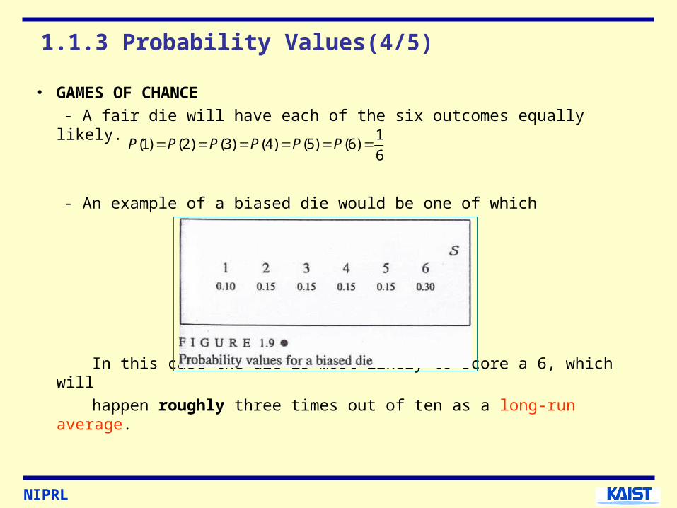
1.3.1 Intersections of Events(5/5)
A B A
( ) ( )
A B B A
A A A
A S A
A
A A
A B C A B C

NIPRL
1.3.2 Unions of Events(1/4)
• Unions of Events The event is the union of events A and B and
consists of the outcomes that are contained within at least one of the events A and B. The probability of this event, , is the probability that at least one of the events A and B occurs.
A B
( )P A B

NIPRL
1.3.2 Unions of Events(2/4)
• Notice that the outcomes in the event can be classified into three kinds.
1. in event but not in event 2. in event but not in event or 3. in both events and
A B
A
AA
BB
B
( ) ( ) ( ) ( )P A B P A B P A B P A B

NIPRL
1.3.2 Unions of Events(3/4)
( ) ( ) ( )
( ) ( ) ( )
( ) ( ) ( ) ( )
If the events and are mutually exclusive so that
( ) 0, then ( ) ( ) ( )
P A B P A P A B
P A B P B P A B
P A B P A P B P A B
A B
P A B P A B P A P B
NIPRL
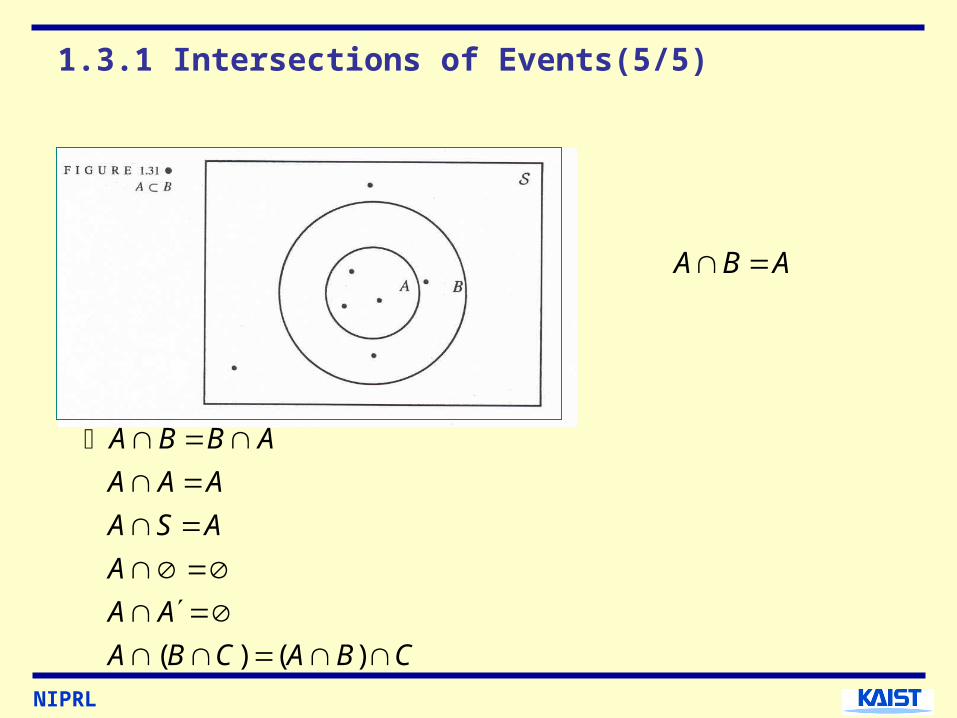
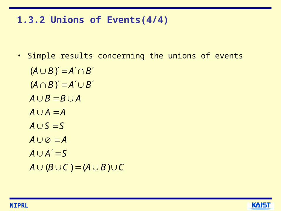
1.3.2 Unions of Events(4/4)
• Simple results concerning the unions of events
( )
( )
( ) ( )
A B A B
A B A B
A B B A
A A A
A S S
A A
A A S
A B C A B C

NIPRL
1.3.3 Examples of Intersections and Unions(1/11)• Example 5 Television Set Quality A company that manufactures television sets performs a
final quality check on each appliance before packing and shipping it.
The quality check has an evaluation of the quality of the picture and the appearance. Each of the two evaluations is graded as Perfect (P), Good (G), Satisfactory (S), or Fail (F).

NIPRL
1.3.3 Examples of Intersections and Unions(2/11) An appliance that fails on either of the two evaluations and
that score an evaluation of Satisfactory on both accounts will not be shipped.
A = { an appliance cannot be shipped } = { (F,P), (F,G), (F,S), (F,F), (P,F), (G,F), (S,F), (S,S) }
P(A) = 0.074
About 7.4% of the television
sets will fail the quality check.

NIPRL
1.3.3 Examples of Intersections and Unions(3/11)
B = { picture satisfactory or fail }
P(B) = 0.178

NIPRL
1.3.3 Examples of Intersections and Unions(4/11) = { Not shipped and the picture satisfactory or fail }A B
( ) 0.055P A B

NIPRL
1.3.3 Examples of Intersections and Unions(5/11) = { the appliance was either not shipped or the
picture was evaluated as being either Satisfactory or Fail }
A B
( ) 0.197P A B

NIPRL
1.3.3 Examples of Intersections and Unions(6/11) = { Television sets that have a picture evaluation of
either Perfect or Good but that cannot be shipped }
( ) 0.019
Notice
( ) ( ) 0.055 0.019
0.074
( )
P A B
P A B P A B
P A
( ')P A B
NIPRL
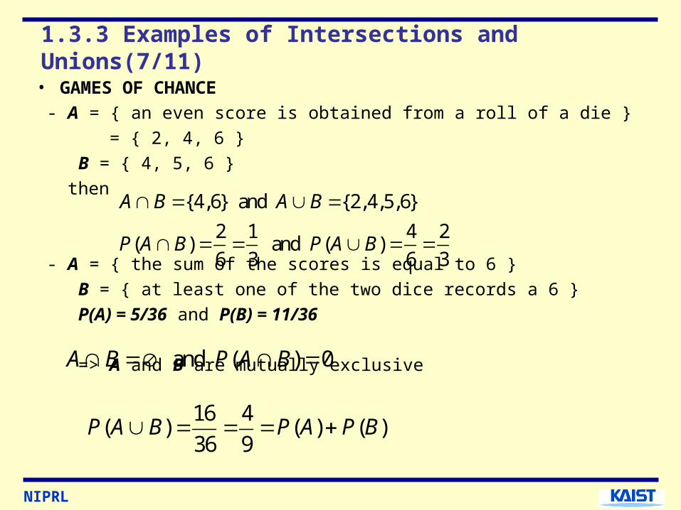
1.3.3 Examples of Intersections and Unions(7/11)• GAMES OF CHANCE - A = { an even score is obtained from a roll of a die } = { 2, 4, 6 } B = { 4, 5, 6 } then
- A = { the sum of the scores is equal to 6 } B = { at least one of the two dice records a 6 } P(A) = 5/36 and P(B) = 11/36
=> A and B are mutually exclusive
{4,6} and {2,4,5,6}
2 1 4 2( ) and ( )
6 3 6 3
A B A B
P A B P A B
and ( ) 0A B P A B
16 4( ) ( ) ( )
36 9P A B P A P B

NIPRL
1.3.3 Examples of Intersections and Unions(8/11)
- One die is red and the other is blue (red, blue). A = { an even score is obtained on the red die }

NIPRL
1.3.3 Examples of Intersections and Unions(9/11)
B = { an even score is obtained on the blue die }

NIPRL
1.3.3 Examples of Intersections and Unions(10/11)
= { both dice have even scores }A B
9 1( )
36 4P A B

NIPRL
1.3.3 Examples of Intersections and Unions(11/11)
= { at least one die has an even score }A B
27 3( )
36 4P A B

NIPRL
1.3.4 Combinations of Three or More Events(1/4)
• Union of Three Events The probability of the union of three events A, B, and C is
the sum of the probability values of the simple outcomes that are contained within at least one of the three events. It can also be calculated from the expression
( ) ( ) ( ) ( )
( ) ( ) ( )
( )
P A B C P A P B P C
P A B P A C P B C
P A B C

NIPRL
1.3.4 Combinations of Three or More Events(2/4)
( ) ( ) ( ) ( )P A B C P A P B P C

NIPRL
1.3.4 Combinations of Three or More Events(3/4)• Union of Mutually Exclusive Events For a sequence of mutually exclusive events,
the probability of the union of the events is given by
• Sample Space Partitions A partition of a sample space is a sequence of mutually exclusive events for which
Each outcome in the sample space is then contained within one
and only one of the events
1 2, ,..., nA A A
1 1( ) ( ) ( )n nP A A P A P A
1 2, ,..., nA A A
1 nA A S
iA

NIPRL
1.3.4 Combinations of Three or More Events(4/4)• Example 5 Television Set Quality C = { an appliance is of “mediocre quality” } = { score either Satisfactory or Good } = { (S,S), (S,G), (G,S), (G,G) } D = { an appliance is of “ high quality” } = = { (G,P), (P,P), (P,G), (P,S) } P(D) = 0.523
( )A B C A B C

NIPRL
1.4 Conditional Probability1.4.1 Definition of Conditional Probability(1/2)• Conditional Probability The conditional probability of event A conditional on
event B is
for P(B)>0. It measures the probability that event A occurs
when it is known that event B occurs.
( )( | )
( )
P A BP A B
P B
( ) 0( | ) 0
( ) ( )
( ) ( )( | ) 1
( ) ( )
A B
P A BP A B
P B P B
B A
A B B
P A B P BP A B
P B P B

NIPRL
1.4.1 Definition of Conditional Probability(2/2)
( ) 0.26( | ) 0.464
( ) 0.56
( ) ( ) ( ) 0.27 0.26( | ) 0.023
( ) 1 ( ) 1 0.56
( | ) ( | ) 1
Formally,
( ) ( )( | ) ( | )
( ) ( )
1 1( ( ) ( )) ( ) 1
( ) ( )
( |
P A BP A B
P B
P A B P A P A BP A B
P B P B
P A B P A B
P A B P A BP A B P A B
P B P B
P A B P A B P BP B P B
P A
( ( ))
)( )
P A B CB C
P B C

NIPRL
1.4.2 Examples of Conditional Probabilities(1/3)• Example 4 Power Plant Operation A = { plant X is idle } and P(A) = 0.32 Suppose it is known that at least two out of the three plants are generating electricity ( event B ). B = { at least two out of the three plants generating electricity }
P(A) = 0.32 => P(A|B) = 0.257
( ) 0.18( | ) 0.257
( ) 0.70
P A BP A B
P B

NIPRL
1.4.2 Examples of Conditional Probabilities(2/3)• GAMES OF CHANCE - A fair die is rolled.
- A red die and a blue die are thrown. A = { the red die scores a 6 } B = { at least one 6 is obtained on the two dice }
1(6)
6(6 ) (6)
(6 | )( ) ( )
(6) 1/ 6 1
(2) (4) (6) 1/ 6 1/ 6 1/ 6 3
P
P even PP even
P even P even
P
P P P
6 1 11( ) and ( )
36 6 36( )
( | )( )
( )
( )
1/ 6 6
11/ 36 11
P A P B
P A BP A B
P B
P A
P B

NIPRL
1.4.2 Examples of Conditional Probabilities(3/3)
C = { exactly one 6 has been scored }
( )( | )
( )
5 / 36 1
10 / 36 2
P A CP A C
P C

NIPRL
1.5 Probabilities of Event Intersections1.5.1 General Multiplication Law
• Probabilities of Event Intersections The probability of the intersection of a series of events can be calculated from the expression
( )( | )
( )
( )( | )
( )
( ) ( ) ( | ) ( ) ( | )
( )( | )
( )
( ) ( ) ( | )) ( ) ( | ) ( | )
P A BP A B
P B
P A BP B A
P A
P A B P B P A B P A P B A
P A B CP C A B
P A B
P A B C P A B P C A B P A P B A P C A B
1 2, ,..., nA A A
1 1 2 1 1 1( ) ( ) ( | ) ( | )n n nP A A P A P A A P A A A

NIPRL
1.5.2 Independent Events
• Independent Events Two events A and B are said to be
independent events if one of the following holds:
Any one of these conditions implies the other two.
( | ) ( )
( ) ( ) ( | ) ( ) ( )
( ) ( ) ( )and ( | ) ( )
( ) ( )
P B A P B
P A B P A P B A P A P B
P A B P A P BP A B P A
P B P B
( | ) ( ), ( | ) ( ), and ( ) ( ) ( )P A B P A P B A P B P A B P A P B

NIPRL
• The interpretation of two events being independent is that knowledge about one event does not affect the probability of the other event.
• Intersections of Independent Events The probability of the intersection of a
series of independent events is simply given by
1 2, ,..., nA A A
1 1 2( ) ( ) ( ) ( )n nP A A P A P A P A

NIPRL
1.5.3 Examples and Probability Trees(1/3)
• Example 7: Car Warranties A company sells a certain type of car, which it assembles in
one of four possible locations. Plant I supplies 20%; plant II, 24%; plant III, 25%; and plant IV, 31%. A customer buying a car does not know where the car has been assembled, and so the probabilities of a purchased car being from each of the four plants can be thought of as being 0.20, 0.24, 0.25, and 0.31.
Each new car sold carries a 1-year bumper-to-bumper warranty.
P( claim | plant I ) = 0.05, P( claim | plant II ) = 0.11 P( claim | plant III ) = 0.03, P( claim | plant IV ) = 0.08 For example, a car assembled in plant I has a probability of
0.05 of receiving a claim on its warranty. Notice that claims are clearly not independent of
assembly location because these four conditional probabilities are unequal.

NIPRL
1.5.3 Examples and Probability Trees(2/3) P( claim ) = P( plant I, claim ) + P( plant II, claim ) + P( plant III, claim) + P( plant IV, claim ) = 0.0687
NIPRL
1.5.3 Examples and Probability Trees(3/3)
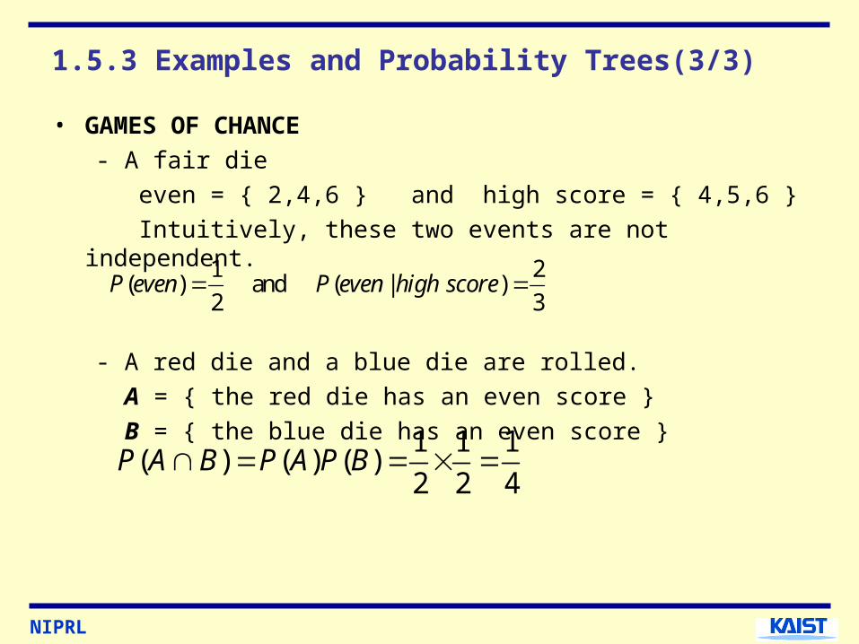
• GAMES OF CHANCE - A fair die even = { 2,4,6 } and high score = { 4,5,6 } Intuitively, these two events are not independent.
- A red die and a blue die are rolled. A = { the red die has an even score } B = { the blue die has an even score }
1 2( ) and ( | )
2 3P even P even high score
1 1 1( ) ( ) ( )
2 2 4P A B P A P B

NIPRL
1.6 Posterior Probabilities1.6.1 Law of Total Probability(1/3)
1
1
1
1 1
{1,2,3,4,5,6}
and : mutually exclusive
( ) ( ) and ( ) : mutually exclusive
( ) ( ) ( )
( ) ( | ) ( ) ( | )
n i
n i
n
n n
S
S A A A
B A B A B A B
P B P A B P A B
P A P B A P A P B A

NIPRL
1.6.1 Law of Total Probability(2/3)
• Law of Total Probability If is a partition of a sample space, then the
probability of an event B can be obtained from the probabilities
and using the formula1 1( ) ( ) ( | ) ( ) ( | )n nP B P A P B A P A P B A
1 2, ,..., nA A A
( )iP A ( | )iP B A

NIPRL
1.6.1 Law of Total Probability(3/3)
• Example 7 Car Warranties If are, respectively, the events that a car is
assembled in plants I, II, III, and IV, then they provide a partition of the sample space, and the probabilities are the supply proportions of the four plants.
B = { a claim is made } = the claim rates for the four individual plants
1 2 3 4, , , and A A A A
( )iP A
1 1 2 2 3 3 4 4( ) ( ) ( | ) ( ) ( | ) ( ) ( | ) ( ) ( | )
(0.20 0.05) (0.24 0.11) (0.25 0.03) (0.31 0.08)
0.0687
P B P A P B A P A P B A P A P B A P A P B A

NIPRL
1.6.2 Calculation of Posterior Probabilities
• Bayes’ Theorem If is a partition of a sample space, then the
posterior probabilities of the event conditional on an event B can be obtained from the probabilities and using the formula
1
1
1
( ) and ( | ) ( | ) ?
( ), , ( ) : the prior probabilities
( | ), , ( | ) : the posterior probabilities
( ) ( ) ( | ) ( ) ( | )( | )
( ) ( ) ( ) ( | )
i i i
n
n
i i i i ii n
j jj
P A P B A P A B
P A P A
P A B P A B
P A B P A P B A P A P B AP A B
P B P B P A P B A
1 2, ,..., nA A A
( )iP A ( | )iP B A
1
( ) ( | )( | )
( ) ( | )
i ii n
j jj
P A P B AP A B
P A P B A
iA

NIPRL
1.6.3 Examples of Posterior Probabilities(1/2)
• Example 7 Car Warranties - The prior probabilities
- If a claim is made on the warranty of the car, how does this change these probabilities?
( ) 0.20, ( ) 0.24
( ) 0.25, ( ) 0.31
P plant I P plant II
P plant III P plant IV
( ) ( | ) 0.20 0.05( | ) 0.146
( ) 0.0687
( ) ( | ) 0.24 0.11( | ) 0.384
( ) 0.0687
( ) ( | ) 0.( | )
( )
P plant I P claim plant IP plant I claim
P claim
P plant II P claim plant IIP plant II claim
P claim
P plant III P claim plant IIIP plant III claim
P claim
25 0.03
0.1090.0687
( ) ( | ) 0.31 0.08( | ) 0.361
( ) 0.0687
P plant IV P claim plant IVP plant IV claim
P claim

NIPRL
1.6.3 Examples of Posterior Probabilities(2/2)
- No claim is made on the warranty
( ) ( | )( | )
( )
0.20 0.950.204
0.9313( ) ( | )
( | )( )
0.24 0.890.229
0.9313( ) ( |
( | )
P plant I P no claim plant IP plant I no claim
P no claim
P plant II P no claim plant IIP plant II no claim
P no claim
P plant III P no claim planP plant III no claim
)
( )
0.25 0.970.261
0.9313( ) ( | )
( | )( )
0.31 0.920.306
0.9313
t III
P no claim
P plant IV P no claim plant IVP plant IV no claim
P no claim