Nick Kaiser

Pan-STARRS, Institute for Astronomy, U. Hawaii

Following the Photons

Edinburgh, Oct 10, 2011

Configuring the Pan-STARRS Optics-

From Simulations to Operational Control System

2

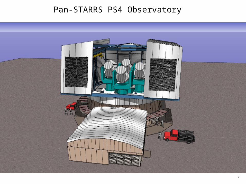
Pan-STARRS PS4 Observatory

3

4

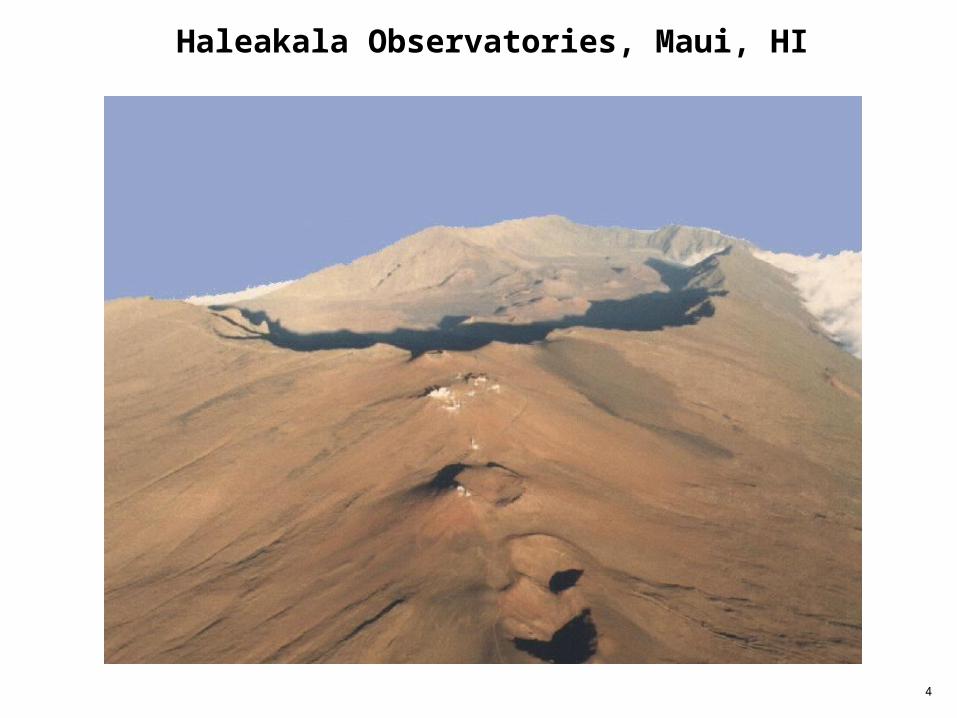
Haleakala Observatories, Maui, HI

5

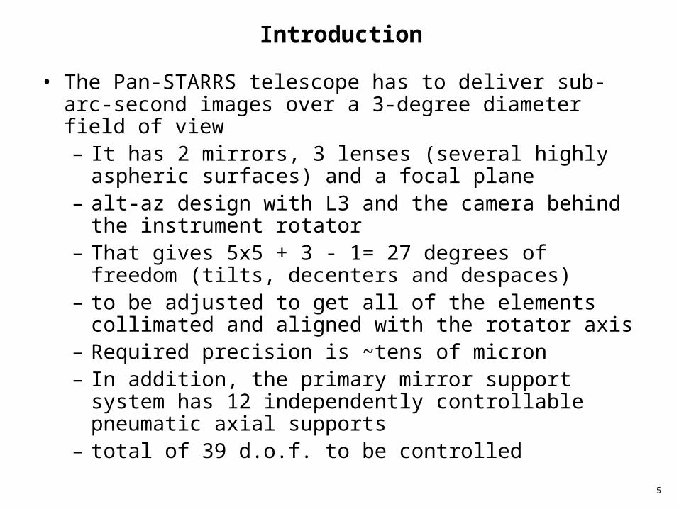
Introduction

• The Pan-STARRS telescope has to deliver sub-arc-second images over a 3-degree diameter field of view– It has 2 mirrors, 3 lenses (several highly aspheric

surfaces) and a focal plane– alt-az design with L3 and the camera behind the

instrument rotator– That gives 5x5 + 3 - 1= 27 degrees of freedom (tilts,

decenters and despaces)– to be adjusted to get all of the elements collimated

and aligned with the rotator axis– Required precision is ~tens of micron– In addition, the primary mirror support system has 12

independently controllable pneumatic axial supports– total of 39 d.o.f. to be controlled

6

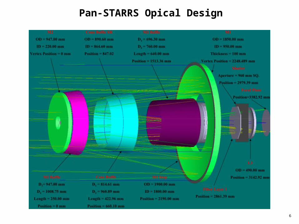
Pan-STARRS Opical Design

7

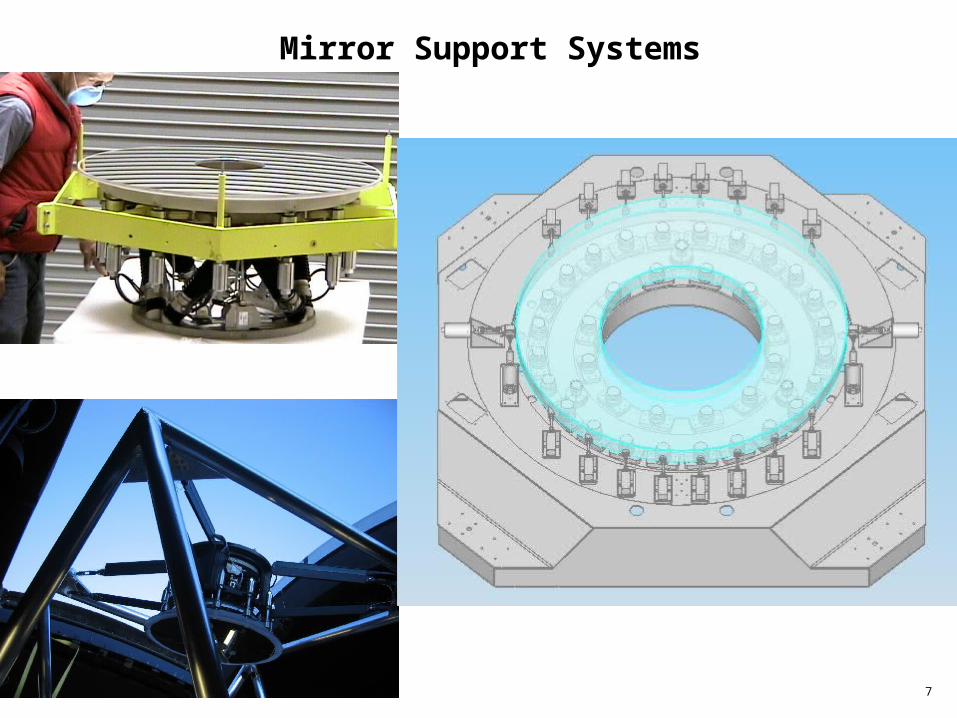
Mirror Support Systems

8

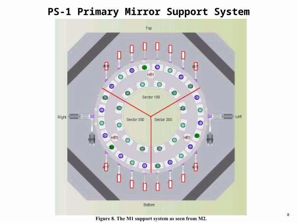
PS-1 Primary Mirror Support System

9

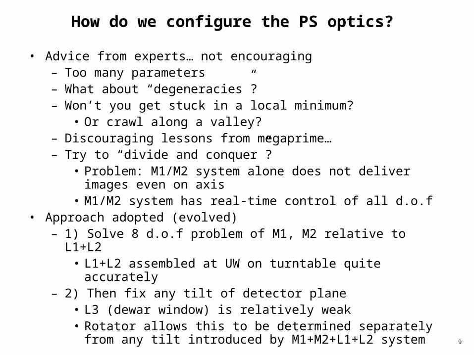
How do we configure the PS optics?

• Advice from experts… not encouraging– Too many parameters– What about “degeneracies”?– Won’t you get stuck in a local minimum?

• Or crawl along a valley?– Discouraging lessons from megaprime…– Try to “divide and conquer”?

• Problem: M1/M2 system alone does not deliver images even on axis

• M1/M2 system has real-time control of all d.o.f• Approach adopted (evolved)

– 1) Solve 8 d.o.f problem of M1, M2 relative to L1+L2• L1+L2 assembled at UW on turntable quite accurately

– 2) Then fix any tilt of detector plane• L3 (dewar window) is relatively weak• Rotator allows this to be determined separately from any tilt

introduced by M1+M2+L1+L2 system

10

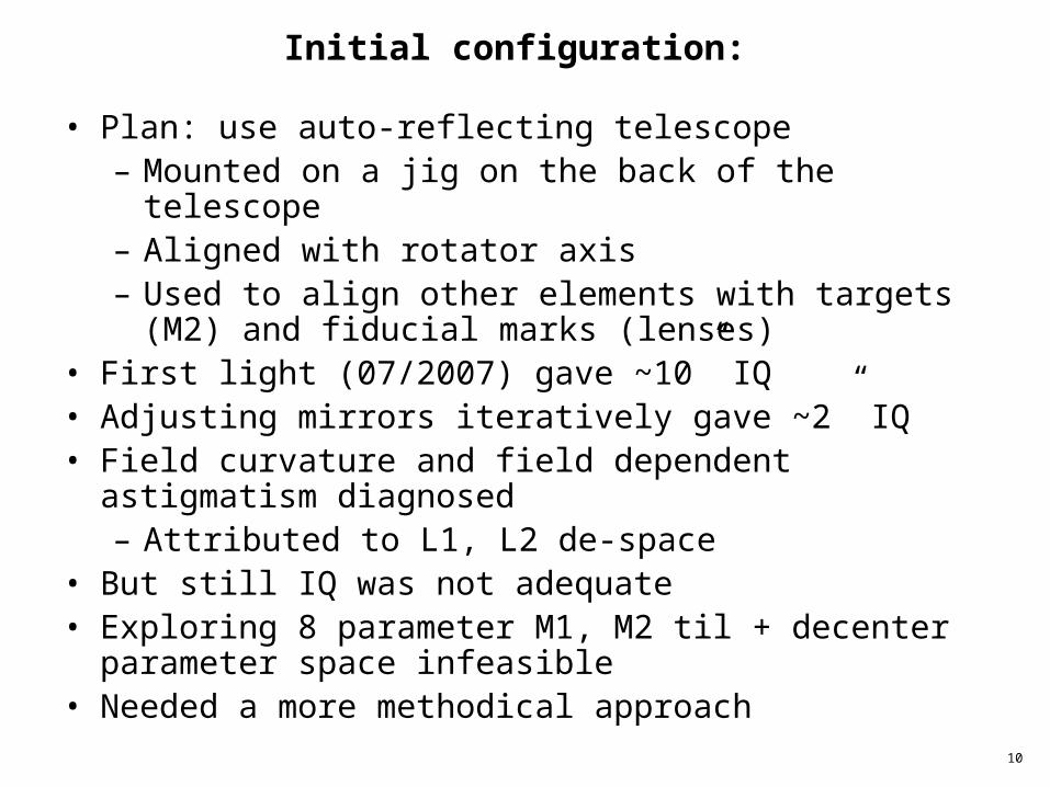
Initial configuration:

• Plan: use auto-reflecting telescope– Mounted on a jig on the back of the telescope– Aligned with rotator axis– Used to align other elements with targets (M2) and

fiducial marks (lenses)• First light (07/2007) gave ~10” IQ• Adjusting mirrors iteratively gave ~2” IQ• Field curvature and field dependent astigmatism

diagnosed– Attributed to L1, L2 de-space

• But still IQ was not adequate• Exploring 8 parameter M1, M2 til + decenter parameter

space infeasible• Needed a more methodical approach

11

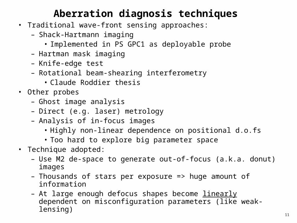
Aberration diagnosis techniques • Traditional wave-front sensing approaches:

– Shack-Hartmann imaging• Implemented in PS GPC1 as deployable probe

– Hartman mask imaging– Knife-edge test– Rotational beam-shearing interferometry

• Claude Roddier thesis• Other probes

– Ghost image analysis– Direct (e.g. laser) metrology– Analysis of in-focus images

• Highly non-linear dependence on positional d.o.fs• Too hard to explore big parameter space

• Technique adopted:– Use M2 de-space to generate out-of-focus (a.k.a. donut) images– Thousands of stars per exposure => huge amount of information– At large enough defocus shapes become linearly dependent on

misconfiguration parameters (like weak-lensing)

12

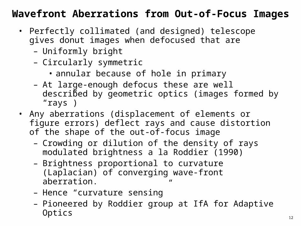
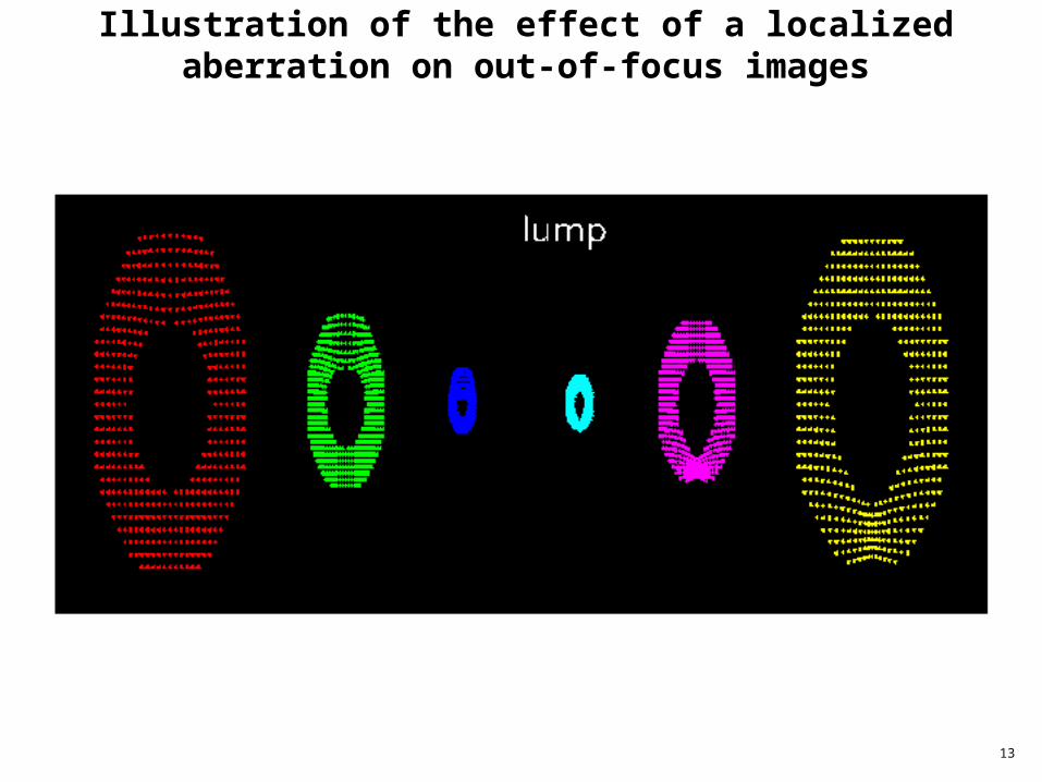
Wavefront Aberrations from Out-of-Focus Images

• Perfectly collimated (and designed) telescope gives donut images when defocused that are– Uniformly bright– Circularly symmetric

• annular because of hole in primary– At large-enough defocus these are well described by geometric

optics (images formed by “rays”)• Any aberrations (displacement of elements or figure errors) deflect

rays and cause distortion of the shape of the out-of-focus image– Crowding or dilution of the density of rays modulated brightness

a la Roddier (1990)– Brightness proportional to curvature (Laplacian) of converging

wave-front aberration.– Hence “curvature sensing”– Pioneered by Roddier group at IfA for Adaptive Optics

13

Illustration of the effect of a localized aberration on out-of-focus images

14

Advantages: Linearity and Multiplexing

• Donut shape statistics are a linear response to causes of aberrations– Linearity breaks down too close to focus.– Shadowing and flat fielding etc. become problematic

too far from focus.– `Sweet spot' seems to be around 3mm defocus– may be possible to go closer for more sensitivity

• But may require `physical optics' modelling• Solve a set of linear equations to find mirror

displacements and actuator commands to cancel aberration– No iteration (in principal) - one step solution– No local minima - finds unique global minumum– Massively multiplexed - thousands of stars per image

15

Separating Seeing and Mirror Wobbling from Aberrations

• We want to obtain sub-seeing aberrations.• But seeing causes wavefront errors of many radians of

phase– Causes donuts to wobble around like jello.– Averages out in long exposures– But leads to smearing.

• Worse still, mirror oscillations will produce persistent anisotropies

• Fortunately, such affects can be readily distinguished by using both pre- and post-focus image pairs.

16

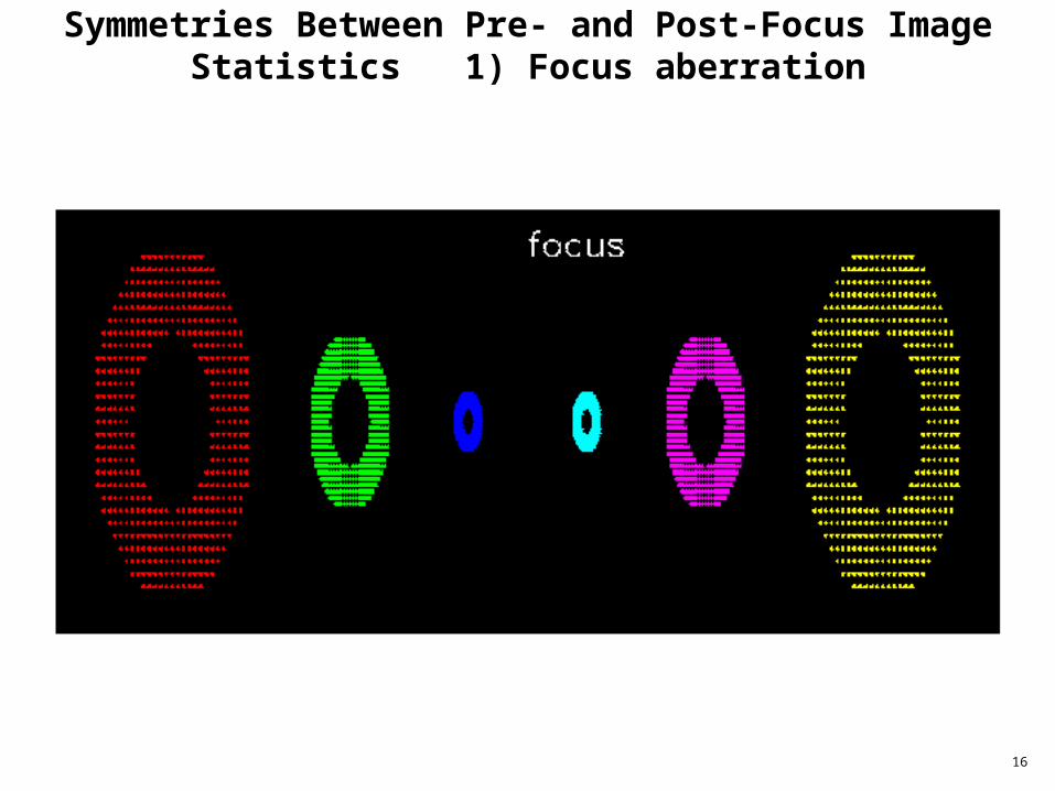
Symmetries Between Pre- and Post-Focus Image Statistics 1) Focus aberration

17

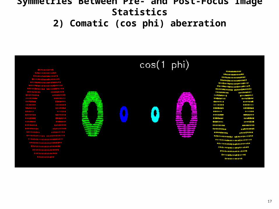
Symmetries Between Pre- and Post-Focus Image Statistics2) Comatic (cos phi) aberration

18

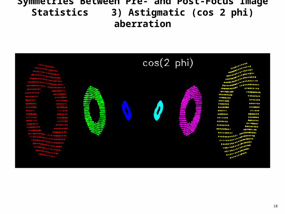
Symmetries Between Pre- and Post-Focus Image Statistics 3) Astigmatic (cos 2 phi) aberration

19

Symmetries and anti-symmetries

• Even angular harmonic change sign passing through focus, while the odd harmonics do not

• If we rotate the post focus images by 180 degrees the sign always changes

• This is the characteristic of wave-front phase errors• But wavefront amplitude errors have opposite symmetry

– Easily distinguished– Can construct combinations of pre- and post focus

image statistics that are blind to effects of telescope wobble, obscurations etc.

20

What about “degeneracies”?

• `Degeneracy' here means combinations of displacements that do not cause any measurable aberration

– Terminology is sloppy: Technically, `degeneracy' means non-distinct eigenvalues

– Here all decenter/tilts are degenerate in the proper sense.

• `Quasi-degeneracy' arises if there are combinations that produce almost zero measurable effect.

– These cause the linear equation solution (inversion of matrix) to be singular or ill conditioned.

– Example: An exact degeneracy arises because IQ only depends on relative positioning of optical elements

– But is easy to deal with

– Quasi-degeneracies are a little more tricky.

21

Dealing with quasi-degeneracies

• Example: decenters and/or tilts of M1 nearly degenerate with decenter of M2

• Similar degeneracies for L3/focal-plane system• But quasi-degeneracies are not to be feared; they are

our friends– Can be identified using elementary linear algebraic

techniques– They allow one to correct for one misalignment that is

difficult to cure by moving another element or combination of elements that are easier

– Fundamental to Pan-STARRS design• real-time control over the configuration of the mirrors• but not of the other elements -- which will surely

flex/expand etc

22

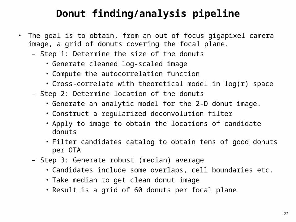
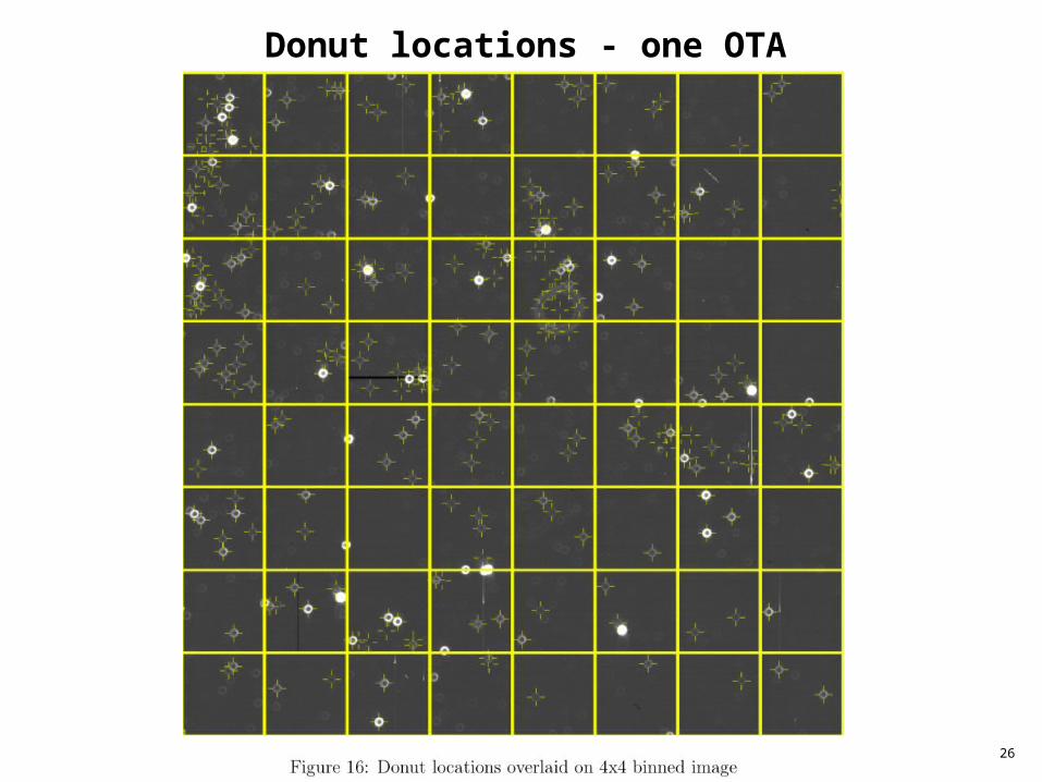
Donut finding/analysis pipeline

• The goal is to obtain, from an out of focus gigapixel camera image, a grid of donuts covering the focal plane.

– Step 1: Determine the size of the donuts

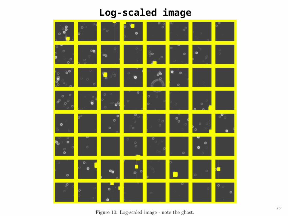
• Generate cleaned log-scaled image

• Compute the autocorrelation function

• Cross-correlate with theoretical model in log(r) space

– Step 2: Determine location of the donuts

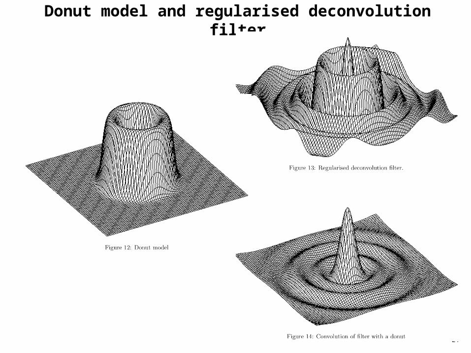
• Generate an analytic model for the 2-D donut image.

• Construct a regularized deconvolution filter

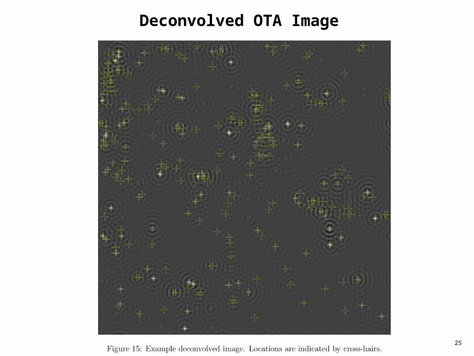
• Apply to image to obtain the locations of candidate donuts

• Filter candidates catalog to obtain tens of good donuts per OTA

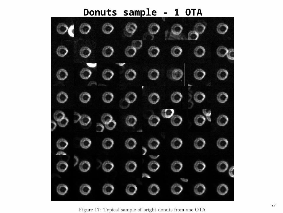
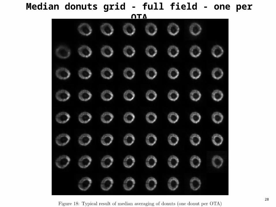
– Step 3: Generate robust (median) average

• Candidates include some overlaps, cell boundaries etc.

• Take median to get clean donut image

• Result is a grid of 60 donuts per focal plane

23

Log-scaled image

24

Donut model and regularised deconvolution filter

25

Deconvolved OTA Image

26

Donut locations - one OTA

27

Donuts sample - 1 OTA

28

Median donuts grid - full field - one per OTA

29

Donut shape statistics

• We need to quantify the distortion of donuts and how this varies across the field.

• What is a good set of statistics?• It is traditional to use Zernike polynomials

– see Knoll, JOSA 66, p207• We use something similar: angular Fourier expansion of radius,

width and brightness of donuts– We first compute the centroid of the light in a postage stamp

containing the donut– From the pixel locations, relative to the centroid, we define a

radius r and azimuthal angle– Compute moments of donut radius, width and brightness

• Typically cos 2, cos 3, cos 4 theta modes– Exploit symmetries in pre- and post-focus images to generate

combined statistic that is independent of actual focus– Results in ~100 statistics for each of ~60 donuts across the focal

plane.

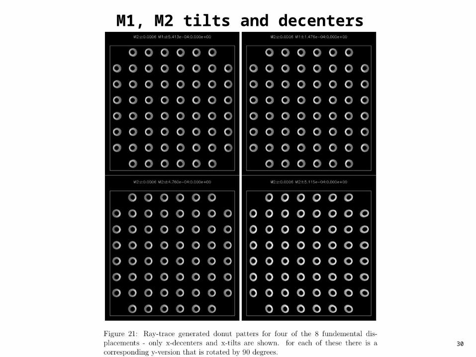
30

M1, M2 tilts and decenters

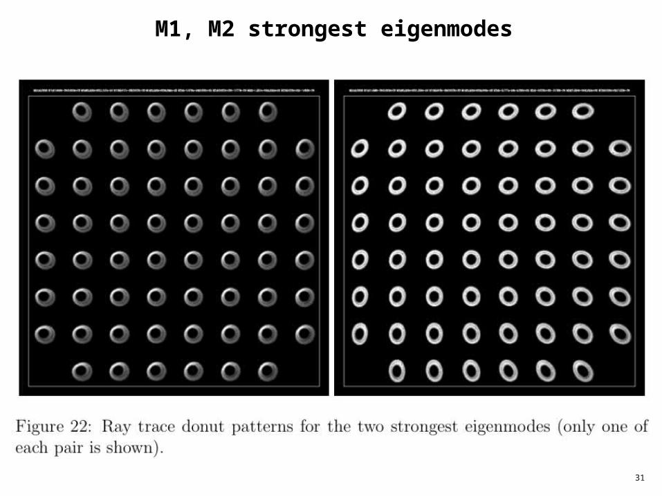
31

M1, M2 strongest eigenmodes

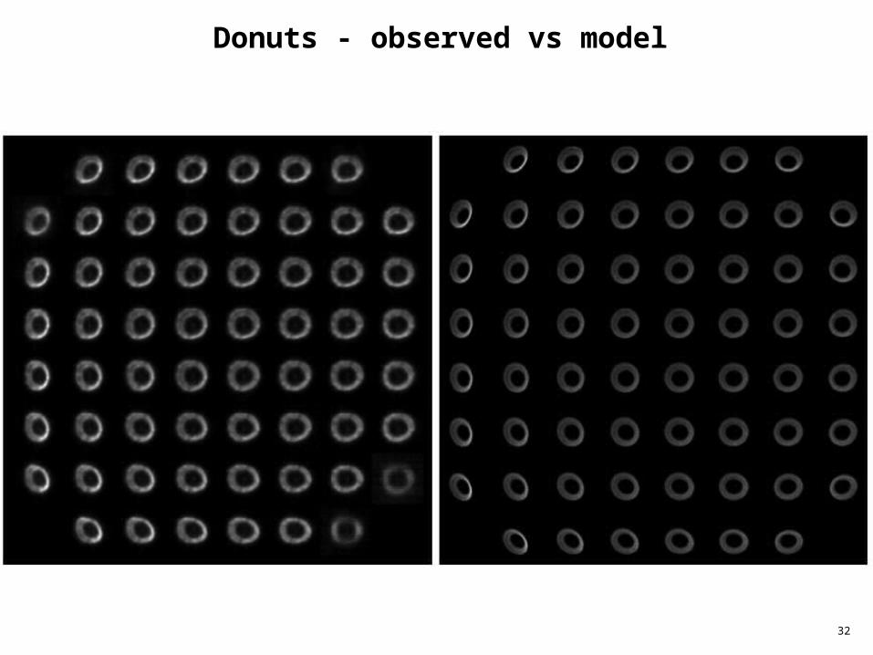
32

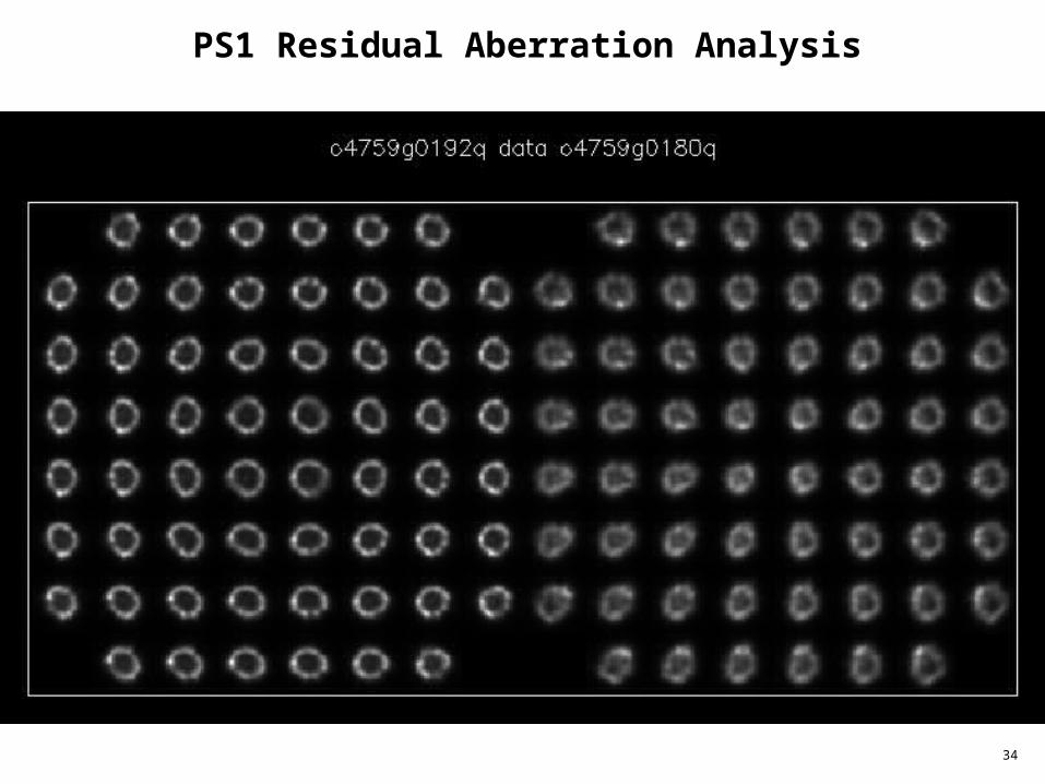
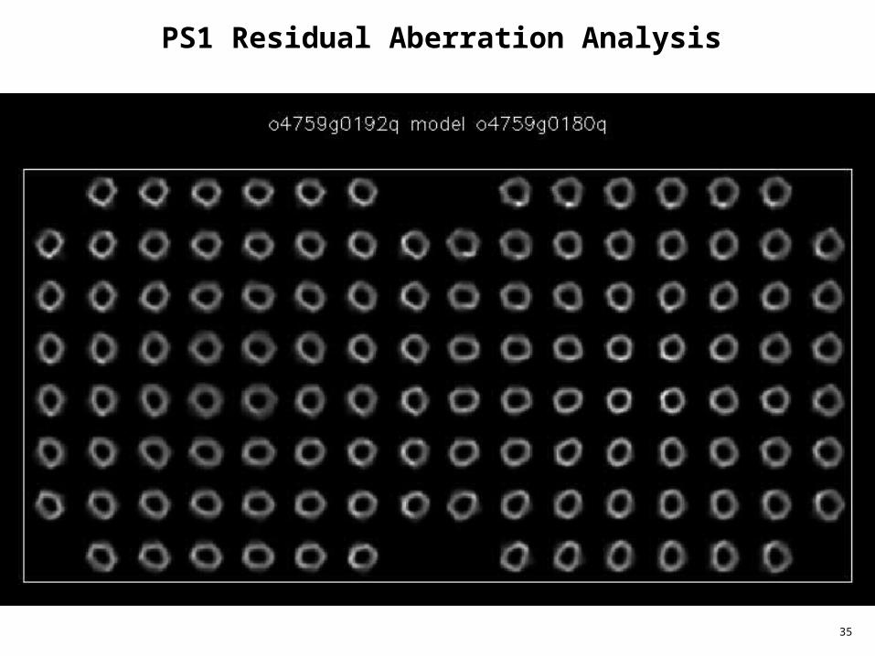
Donuts - observed vs model

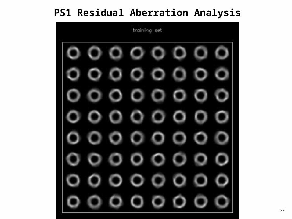
33

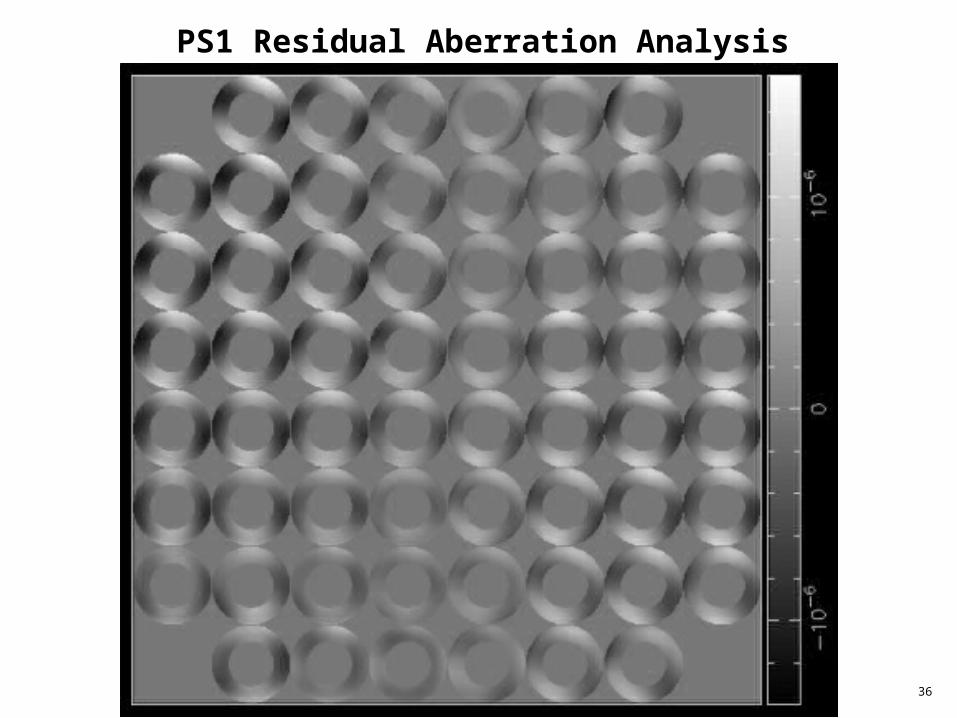
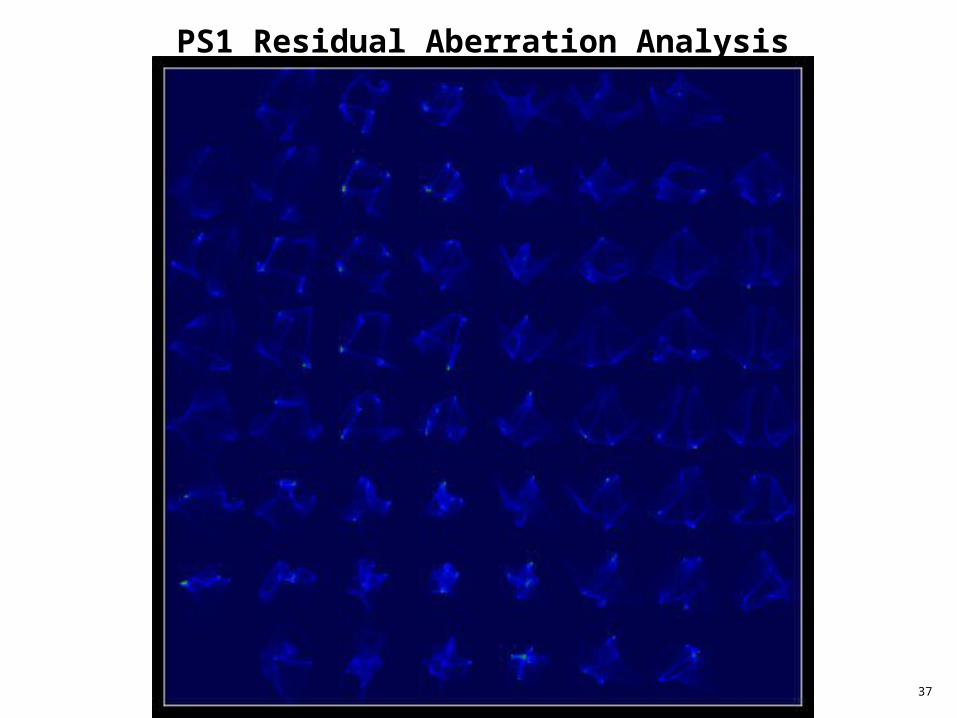
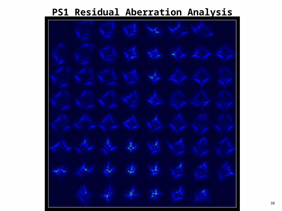
PS1 Residual Aberration Analysis

34

PS1 Residual Aberration Analysis

35

PS1 Residual Aberration Analysis

36

PS1 Residual Aberration Analysis

37

PS1 Residual Aberration Analysis

38

PS1 Residual Aberration Analysis

39UNIVERSITY OF HAWAII INSTITUTE FOR ASTRONOMYProject Proprietary Data – For Internal Use Only

39

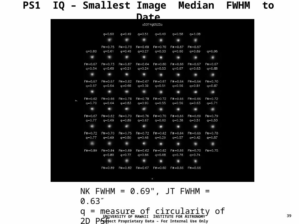
PS1 IQ – Smallest Image Median FWHM to Date

NK FWHM = 0.69", JT FWHM = 0.63 q = measure of circularity of 2D PSF

40

41

42

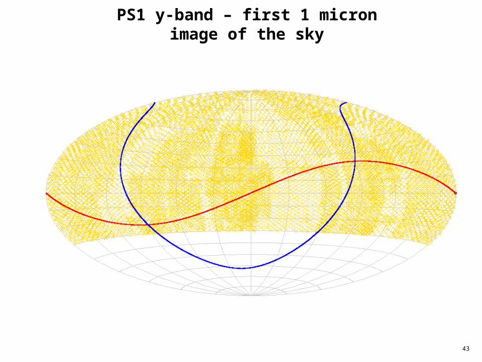
43

PS1 y-band – first 1 micron image of the sky

44

PS1 z, i, r, g band coverage 2011-02-14

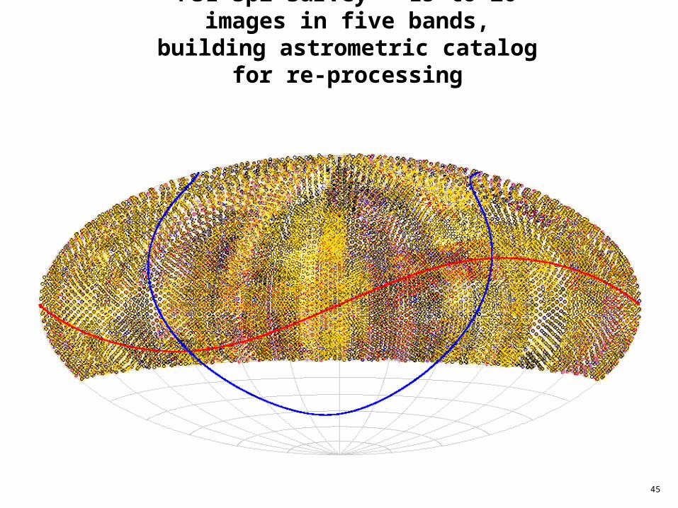
45

PS1 3pi survey – 15 to 20 images in five bands,

building astrometric catalog for re-processing

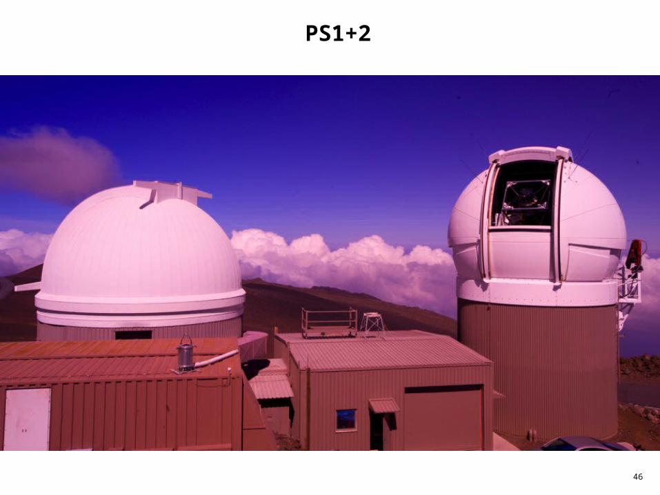
46

PS1+2

47