Neyman-Pearson test for simple binary hypotheses, …namrata/EE527_Spring08/l5c_2.pdf · Outline:...

Outline:

• Neyman-Pearson test for simple binary hypotheses, receiveroperating characteristic (ROC).

• An introduction to classical composite hypothesis testing.

Reading:

• Chapter 3 in Kay-II,

• (part of) Chapter 5 in Levy.

EE 527, Detection and Estimation Theory, # 5c 1

False-alarm and Detection Probabilities forBinary Hypothesis Tests: A Reminder

(see handout # 5)

In binary hypothesis testing, we wish to identify whichhypothesis is true (i.e. make the appropriate decision):

H0 : θ ∈ spΘ(0) null hypothesis versus

H1 : θ ∈ spΘ(1) alternative hypothesis

where

spΘ(0) ∪ spΘ(1) = spΘ, spΘ(0) ∩ spΘ(1) = ∅.

Recall that a binary decision rule φ(x) maps X︸︷︷︸data space

to {0, 1}:

φ(x) ={

1, decide H1,0, decide H0.

which partitions the data space X [i.e. the support offX |Θ(x | θ)] into two regions:

X0 = {x : φ(x) = 0} and X1 = {x : φ(x) = 1}.


Recall the probabilities of false alarm and miss:

PFA(φ(X), θ) = E X |Θ[φ(X) | θ]

=∫X1

fX |Θ(x | θ) dx for θ ∈ spΘ(0) (1)

PM(φ(X), θ) = E X |Θ[1− φ(X) | θ]

= 1−∫X1

fX |Θ(x | θ) dx︸︷︷︸PD(φ(X),θ)

=∫X0

fX |Θ(x | θ) dx for θ in spΘ(1) (2)

and the probability of detection (correctly deciding H1):

PD(φ(X), θ) = E X |Θ[φ(X) | θ] =∫X1

fX |Θ(x | θ) dx for θ in spΘ(1).

For simple hypotheses, spΘ(0) = {θ0}, spΘ(1) = {θ1}, andspΘ = {θ0, θ1}, the above expressions simplify, as shown in thefollowing.


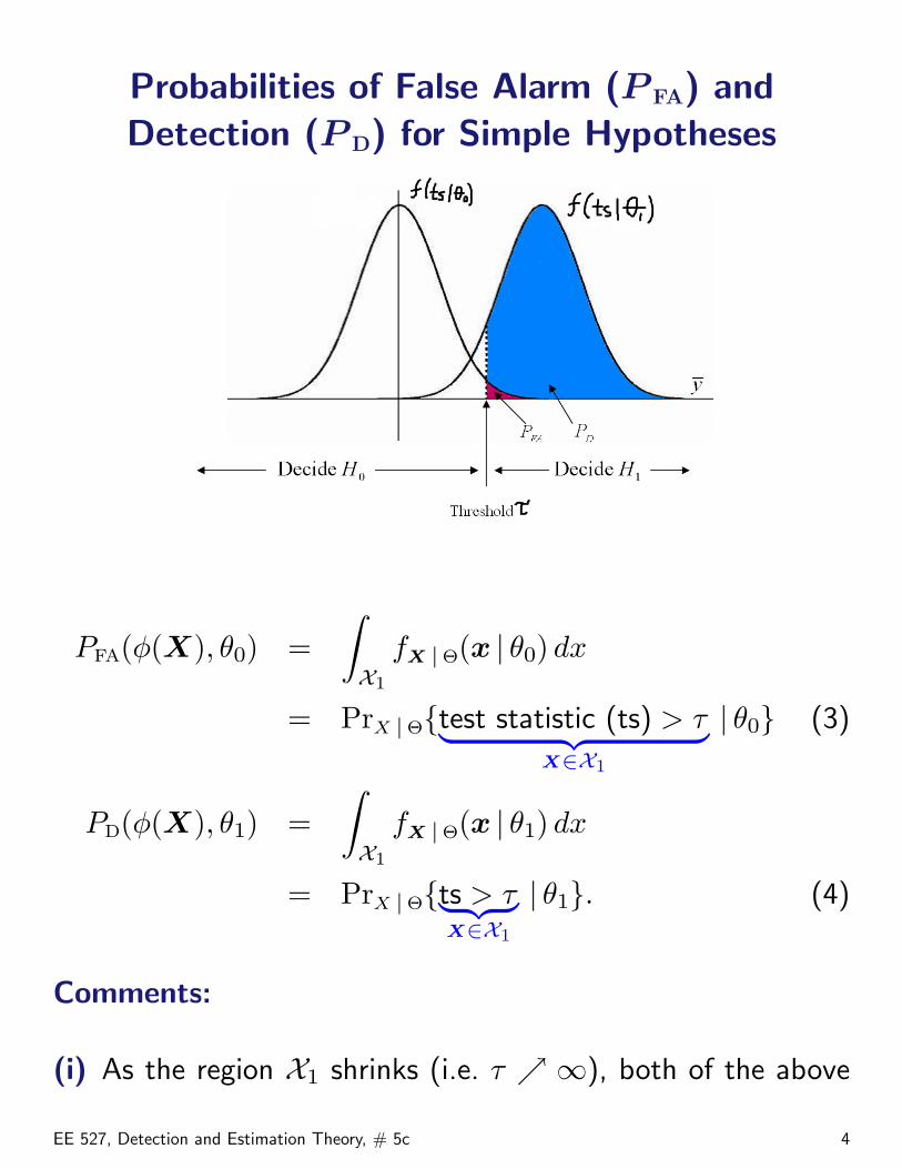
Probabilities of False Alarm (P FA) andDetection (P D) for Simple Hypotheses

PFA(φ(X), θ0) =∫X1

fX |Θ(x | θ0) dx

= PrX |Θ{test statistic (ts) > τ︸︷︷︸X∈X1

| θ0} (3)

PD(φ(X), θ1) =∫X1

fX |Θ(x | θ1) dx

= PrX |Θ{ts > τ︸︷︷︸X∈X1

| θ1}. (4)

Comments:

(i) As the region X1 shrinks (i.e. τ ↗ ∞), both of the above


probabilities shrink towards zero.

(ii) As the region X1 grows (i.e. τ ↘ 0), both probabilitiesgrow towards unity.

(iii) Observations (i) and (ii) do not imply equality betweenPFA and PD; in most cases, as X1 grows, PD grows morerapidly than PFA (i.e. we better be right more often than weare wrong).

(iv) However, the perfect case where our rule is always rightand never wrong (PD = 1 and PFA = 0) cannot occur whenthe conditional pdfs/pmfs fX |Θ(x | θ0) and fX |Θ(x | θ1)overlap.

(v) Thus, to increase the detection probability PD, we mustalso allow for the false-alarm probability PFA to increase.This behavior

• represents the fundamental tradeoff in hypothesis testingand detection theory and

• motivates us to introduce a (classical) approach to testingsimple hypotheses, pioneered by Neyman and Pearson, tobe discussed next.

Receiver Operating Characteristic (ROC) allows us to visualizethe realm of achievable PFA(φ(X), θ0) and PD(φ(X), θ1).


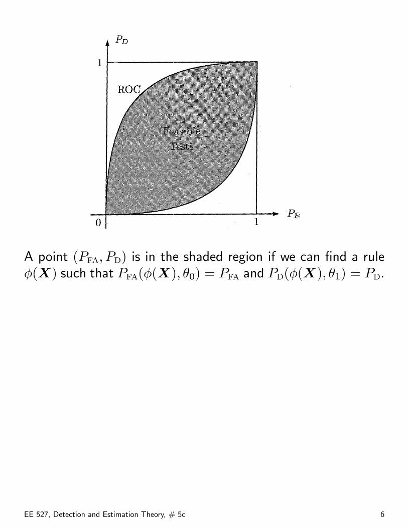
A point (PFA, PD) is in the shaded region if we can find a ruleφ(X) such that PFA(φ(X), θ0) = PFA and PD(φ(X), θ1) = PD.


Neyman-Pearson Test for Simple Hypotheses

Bayesian tests are criticized because they require specificationof prior distribution (pmf or, in the composite-testing case,pdf) and the cost-function parameters L(i | j).

An alternative classical solution for simple hypotheses isdeveloped by Neyman and Pearson.

Select the decision rule φ(X) that maximizesPD(φ(X), θ1) while ensuring that the probability of false alarmPFA(φ(X), θ0) is less than or equal to a specified level α.

Setup:

• Simple hypothesis testing:

H0 : θ = θ0 versus

H1 : θ = θ1.

• Parametric data models fX |Θ(x | θ0), fX |Θ(x | θ1).

• No prior pdf/pmf on Θ is available.


• Define the set of all rules φ(X) whose probability of falsealarm is less than or equal to a specified level α:

Dα ={φ(X)

∣∣PFA(φ(X), θ0) ≤ α}}

see also (3).

A Neyman-Pearson test φNP(x) solves the constrainedoptimization problem:

φNP(x) = arg maxφ(x)∈Dα

PD(φ(x), θ1).

We apply Lagrange multipliers to solve this optimizationproblem; consider the Lagrangian:

L(φ(x), λ) = PD(φ(x), θ1) + λ [α− PFA(φ(x), θ0)]

with λ ≥ 0. A decision rule φ(x) will be optimal if itmaximizes L(φ(x), λ) and satisfies the Karush-Kuhn-Tucker(KKT) condition:

λ [α− PFA(φ(x), θ0)] = 0. (5)

Upon using (3) and (4), the Lagrangian can be written as

L(φ(x), λ) = λ α +∫X1

[fX |Θ(x | θ1)− λ fX |Θ(x | θ0)] dx.


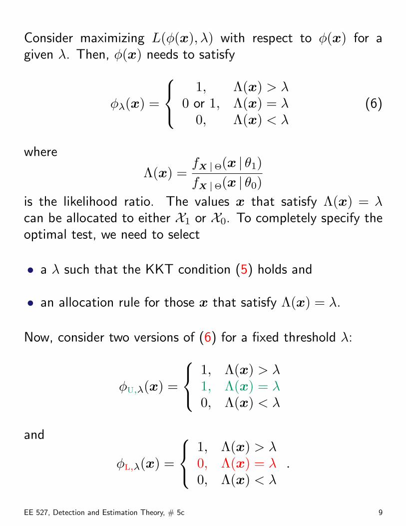
Consider maximizing L(φ(x), λ) with respect to φ(x) for agiven λ. Then, φ(x) needs to satisfy

φλ(x) =

1, Λ(x) > λ0 or 1, Λ(x) = λ

0, Λ(x) < λ(6)

where

Λ(x) =fX |Θ(x | θ1)fX |Θ(x | θ0)

is the likelihood ratio. The values x that satisfy Λ(x) = λcan be allocated to either X1 or X0. To completely specify theoptimal test, we need to select

• a λ such that the KKT condition (5) holds and

• an allocation rule for those x that satisfy Λ(x) = λ.

Now, consider two versions of (6) for a fixed threshold λ:

φU,λ(x) =

1, Λ(x) > λ1, Λ(x) = λ0, Λ(x) < λ

and

φL,λ(x) =

1, Λ(x) > λ0, Λ(x) = λ0, Λ(x) < λ

.


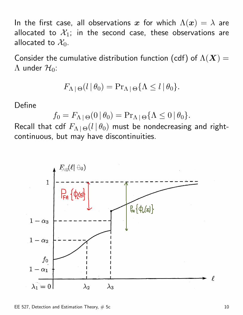
In the first case, all observations x for which Λ(x) = λ areallocated to X1; in the second case, these observations areallocated to X0.

Consider the cumulative distribution function (cdf) of Λ(X) =Λ under H0:

FΛ |Θ(l | θ0) = PrΛ |Θ{Λ ≤ l | θ0}.

Definef0 = FΛ |Θ(0 | θ0) = PrΛ |Θ{Λ ≤ 0 | θ0}.

Recall that cdf FΛ |Θ(l | θ0) must be nondecreasing and right-continuous, but may have discontinuities.


Consider three cases, depending on α:

(i) When1− α < f0 i.e. 1− f0 < α (7)

we select the threshold λ = 0 and apply the rule

φL,0(x) ={

1, Λ(x) > 00, Λ(x) = 0 . (8)

In this case, KKT condition (5) holds and, therefore, thetest (8) is optimal; its probability of false alarm is

PFA(φL,0(x), θ0) = 1− f0 < α see (7).

An example of this case corresponds to λ1 = 0 and 1 − α1

in the above figure.

(ii) Suppose that

1− α ≥ f0 i.e. 1− f0 ≥ α (9)

and there exists a λ such that

FΛ |Θ(λ | θ0) = 1− α. (10)

Then, by selecting this λ as the threshold and using

φL,λ(x) ={

1, Λ(x) > λ0, Λ(x) ≤ λ

(11)


we obtain a test with false-alarm probability

PFA(φL,λ(x), θ0) = 1− FΛ |Θ(λ | θ0) = α see (9)

the KKT condition (5) holds, and the test (10) is optimal.An example of this case corresponds to λ2 and 1−α2 in theabove figure.

(iii) Suppose that

1− α ≥ f0 i.e. 1− f0 ≥ α

as in (ii), but cdf FΛ |Θ(l | θ0) has a discontinuity pointλ > 0 such that

FΛ |Θ(λ− | θ0) < 1− α < FΛ |Θ(λ+ | θ0)

where FΛ |Θ(λ− | θ0) and FΛ |Θ(λ+ | θ0) denote the left andright limits of FΛ |Θ(λ | θ0) at l = λ. If this case happensin practice, we can try to avoid the problem by changingour specified α, which is anyway not God-given, butchosen rather arbitrarily. We should pick a value of αthat satisfies the KKT condition.

Suppose that we are not allowed to change α; this gives usa chance to practice some basic probability. First, note that


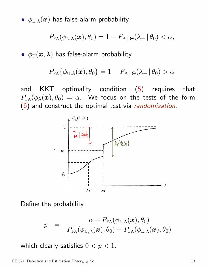
• φL,λ(x) has false-alarm probability

PFA(φL,λ(x), θ0) = 1− FΛ |Θ(λ+ | θ0) < α,

• φU(x, λ) has false-alarm probability

PFA{φU,λ(x), θ0} = 1− FΛ |Θ(λ− | θ0) > α

and KKT optimality condition (5) requires thatPFA(φλ(x), θ0) = α. We focus on the tests of the form(6) and construct the optimal test via randomization.

Define the probability

p =α− PFA(φL,λ(x), θ0)

PFA(φU,λ(x), θ0)− PFA(φL,λ(x), θ0)

which clearly satisfies 0 < p < 1.


Select φU,λ(x) with probability p and φL,λ(x) withprobability 1 − p. This test indeed has the form (6); itsprobability of false alarm is

PFA(φλ(x), θ0)

= PFA(φL,λ(x), θ0) + p [PFA(φU,λ(x), θ0)− PFA(φL,λ(x), θ0)] = α.

Since KKT condition (5) is satisfied, the randomized test

φλ(x) =

1, Λ(x) > λ1 w.p. p and 0 w.p. 1− p, Λ(x) = λ

0, Λ(x) < λ

is optimal.


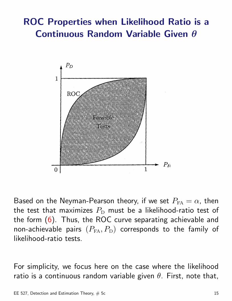
ROC Properties when Likelihood Ratio is aContinuous Random Variable Given θ

Based on the Neyman-Pearson theory, if we set PFA = α, thenthe test that maximizes PD must be a likelihood-ratio test ofthe form (6). Thus, the ROC curve separating achievable andnon-achievable pairs (PFA, PD) corresponds to the family oflikelihood-ratio tests.

For simplicity, we focus here on the case where the likelihoodratio is a continuous random variable given θ. First, note that,


for the likelihood-ratio test,

PFA(τ) =∫X1

fX |Θ(x | θ0) dx

= PrX |Θ{Λ(X) > τ | θ0} =∫ +∞

τ

fΛ |Θ(l | θ0) dl (12)

PD(τ) =∫X1

fX |Θ(x | θ1) dx

= PrX |Θ{Λ(X) > τ | θ1} =∫ +∞

τ

fΛ |Θ(l | θ1) dl (13)

where τ denotes the threshold. Under the continuityassumption for the likelihood ratio, as we vary τ between0 and +∞, the point

(PFA(φ(X), θ0), PD(φ(X), θ1)

)moves

continuously along the ROC curve. If we set τ = 0, we alwaysselect H1 and, therefore,

PFA(0) = PD(0) = 1.

Conversely, if we set τ = +∞, we always select H0 and,therefore,

PFA(+∞) = PD(+∞) = 0.

In summary,

ROC Property 1. If the likelihood ratio is a continuousrandom variable given θ, the points (0, 0) and (1, 1) belong toROC.


Now, differentiate (12) and (13) with respect to τ :

dPD(τ)dτ

= −fΛ |Θ(τ | θ1)

dPD(τ)dτ

= −fΛ |Θ(τ | θ0)

implyingdPD(τ)dPFA(τ)

=fΛ |Θ(τ | θ1)fΛ |Θ(τ | θ0)

= τ.

In summary,

ROC Property 2. If the likelihood ratio is a continuousrandom variable given θ, the slope of ROC at point(PFA(τ), PD(τ)) is equal to the threshold τ of the correspondinglikelihood-ratio test.

In particular, this result implies that the slope of ROC is

• τ = +∞ at (0, 0) and

• τ = 0 at (1, 1).

ROC Property 3. The domain of achievable pairs (PFA, PD)is convex and the ROC curve is concave. This property holdsin general, including the case where the likelihood ratio is amixed or discrete random variable given θ.

HW: Prove ROC Property 3.


ROC Property 4. All points on ROC curve satisfy

PD(τ) ≥ PFA(τ).

This property holds in general, including the case where thelikelihood ratio is a mixed or discrete random variable given θ.


Example: Simple Hypotheses,Coherent Detection in Gaussian Noise with

Known Covariance Matrix

Simple hypotheses: the space of the parameter µ and itspartitions are

spµ = {µ0,µ1}, spµ(0) = {µ0}, spµ(1) = {µ1}.

The measurement vector X given µ is modeled using

fX |µ(x |µ) = N (x |µ, C)

=1√|2 π C|

exp[−12 (x− µ)T C−1 (x− µ)]

where C is a known positive definite covariance matrix. Ourlikelihood-ratio test is

Λ(x)︸︷︷︸likelihood ratio

=fX |µ(x |µ1)fX |µ(x |µ0)

=exp[−1

2 (x− µ1)T C−1 (x− µ1)]exp[−1

2 (x− µ0)T C−1 (x− µ0)

H1

≷ τ.


Therefore,

−12 (x−µ1)

T C−1 (x−µ1)+ 12 (x−µ0)

T C−1 (x−µ0)H1

≷ ln τ

i.e.

(µ1 − µ0)T C−1 [x− 1

2 (µ0 + µ1)]H1

≷ ln τ.

and, finally,

T (x) = sT C−1 xH1

≷ ln τ + 12 (µ1−µ0)

T C−1 (µ1 + µ0)4= γ

where we have defined

s4= µ1 − µ0.

False-alarm and detection/miss probabilities. Given µ,T (x) is a linear combination of Gaussian random variables,implying that it is also Gaussian, with mean and variance:

E X |µ[T (X) |µ] = sT C−1µ

varX |µ[T (X) |µ] = sT C−1s (not a function of µ).


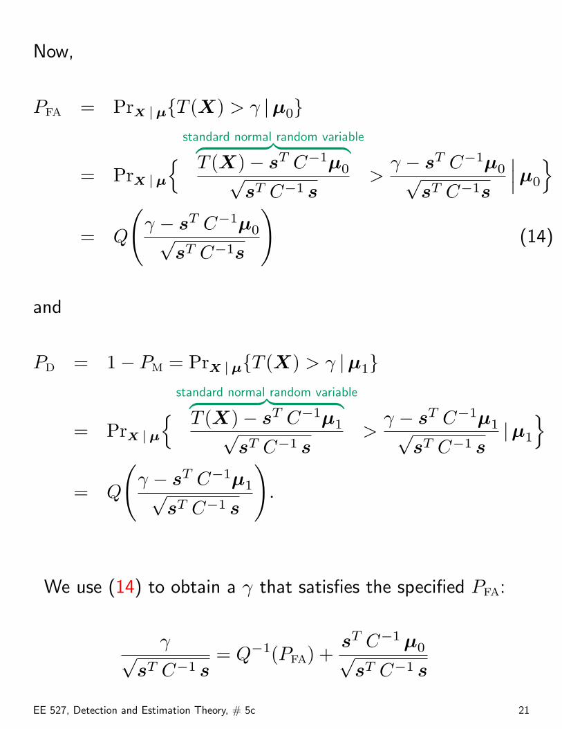
Now,

PFA = PrX |µ{T (X) > γ |µ0}

= PrX |µ

{ standard normal random variable︷︸︸︷T (X)− sT C−1µ0√

sT C−1 s>

γ − sT C−1µ0√sT C−1s

∣∣∣µ0

}= Q

(γ − sT C−1µ0√

sT C−1s

)(14)

and

PD = 1− PM = PrX |µ{T (X) > γ |µ1}

= PrX |µ

{ standard normal random variable︷︸︸︷T (X)− sT C−1µ1√

sT C−1 s>

γ − sT C−1µ1√sT C−1 s

|µ1

}= Q

(γ − sT C−1µ1√

sT C−1 s

).

We use (14) to obtain a γ that satisfies the specified PFA:

γ√sT C−1 s

= Q−1(PFA) +sT C−1 µ0√

sT C−1 s


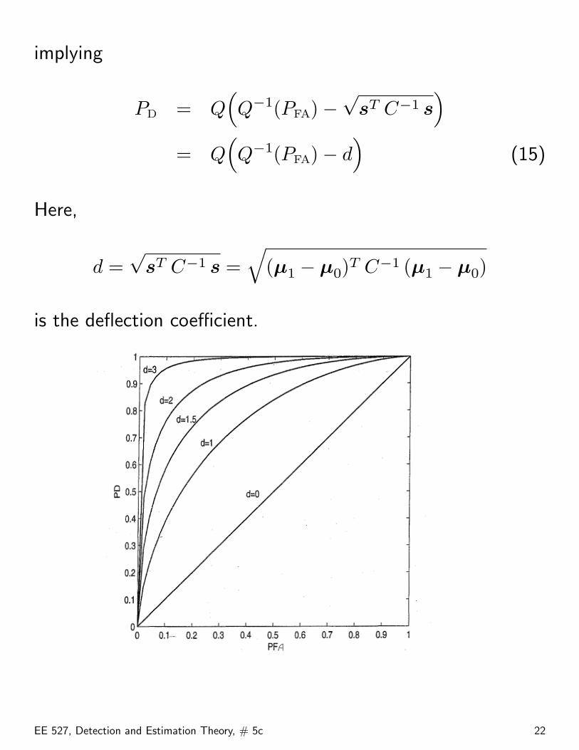
implying

PD = Q(Q−1(PFA)−

√sT C−1 s

)= Q

(Q−1(PFA)− d

)(15)

Here,

d =√

sT C−1 s =√

(µ1 − µ0)T C−1 (µ1 − µ0)

is the deflection coefficient.


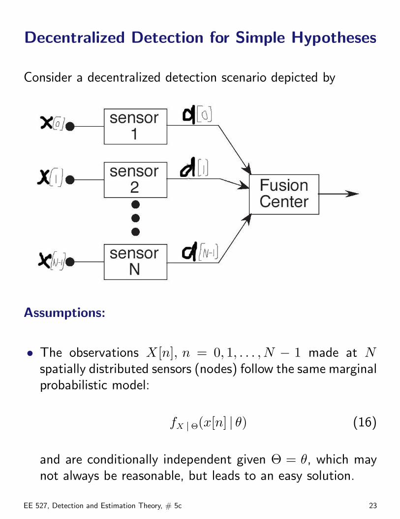
Decentralized Detection for Simple Hypotheses

Consider a decentralized detection scenario depicted by

Assumptions:

• The observations X[n], n = 0, 1, . . . , N − 1 made at Nspatially distributed sensors (nodes) follow the same marginalprobabilistic model:

fX |Θ(x[n] | θ) (16)

and are conditionally independent given Θ = θ, which maynot always be reasonable, but leads to an easy solution.


• We wish to test:

H0 : θ = θ0 versus

H1 : θ = θ1.

• Each node n makes a hard local decision d[n] based onits local observation x[n] and sends it to the headquarters(fusion center), which collects all the local decisions andmakes the final global decision H0 versus H1. This structureis clearly suboptimal: it is easy to construct a betterdecision strategy in which each node sends its (quantized,in practice) likelihood ratio to the fusion center, rather thanthe decision only. However, such a strategy would have ahigher communication (energy) cost.

The false-alarm and detection probabilities of each node’slocal decision rules can be computed using (16). Supposethat we have obtained them for each n:

PFA,n, PD,n, n = 0, 1, . . . , N − 1.

We now discuss the decentralized detection problem. Note that

pD(n) |Θ(dn | θ1) = P dnD,n (1− PD,n)1−dn︸︷︷︸

Bernoulli pmf


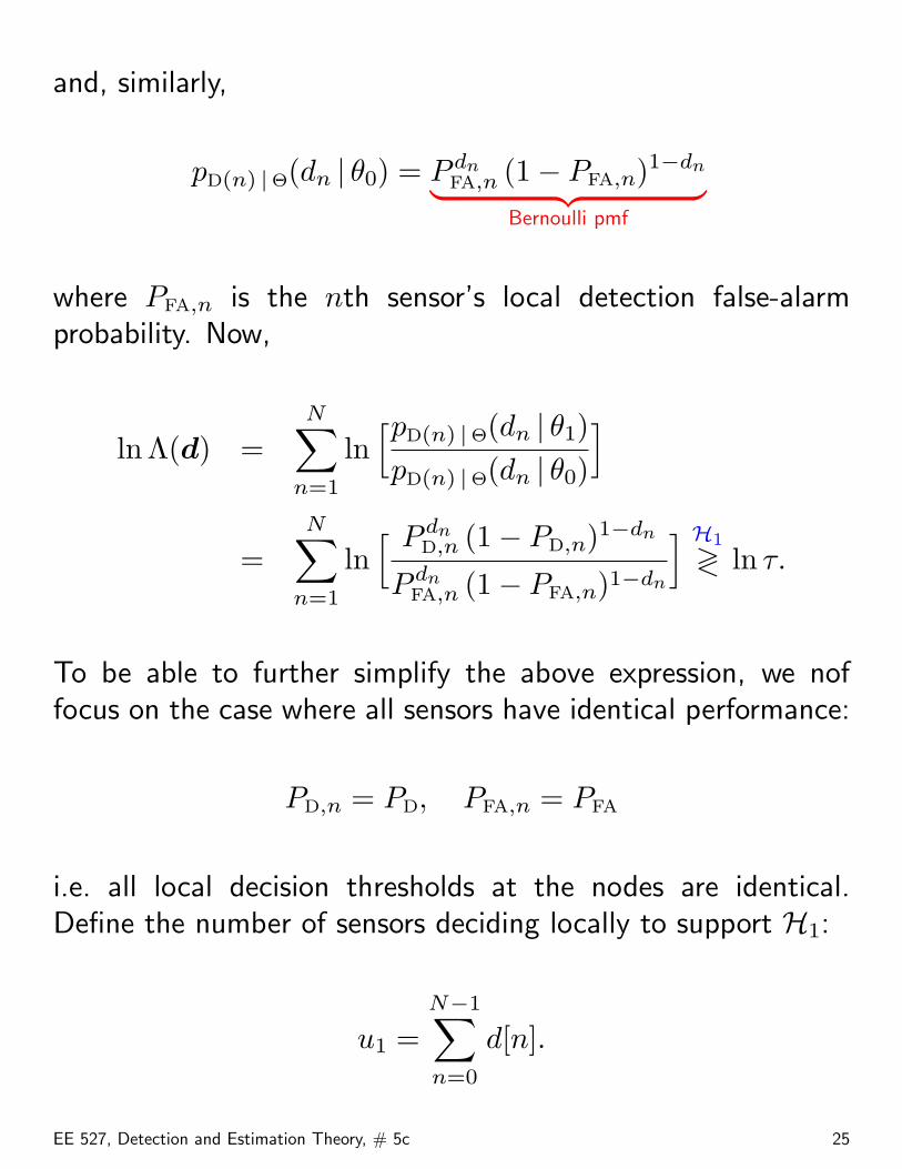
and, similarly,

pD(n) |Θ(dn | θ0) = P dnFA,n (1− PFA,n)1−dn︸︷︷︸

Bernoulli pmf

where PFA,n is the nth sensor’s local detection false-alarmprobability. Now,

lnΛ(d) =N∑

n=1

ln[pD(n) |Θ(dn | θ1)pD(n) |Θ(dn | θ0)

]

=N∑

n=1

ln[ P dn

D,n (1− PD,n)1−dn

P dnFA,n (1− PFA,n)1−dn

] H1

≷ ln τ.

To be able to further simplify the above expression, we noffocus on the case where all sensors have identical performance:

PD,n = PD, PFA,n = PFA

i.e. all local decision thresholds at the nodes are identical.Define the number of sensors deciding locally to support H1:

u1 =N−1∑n=0

d[n].


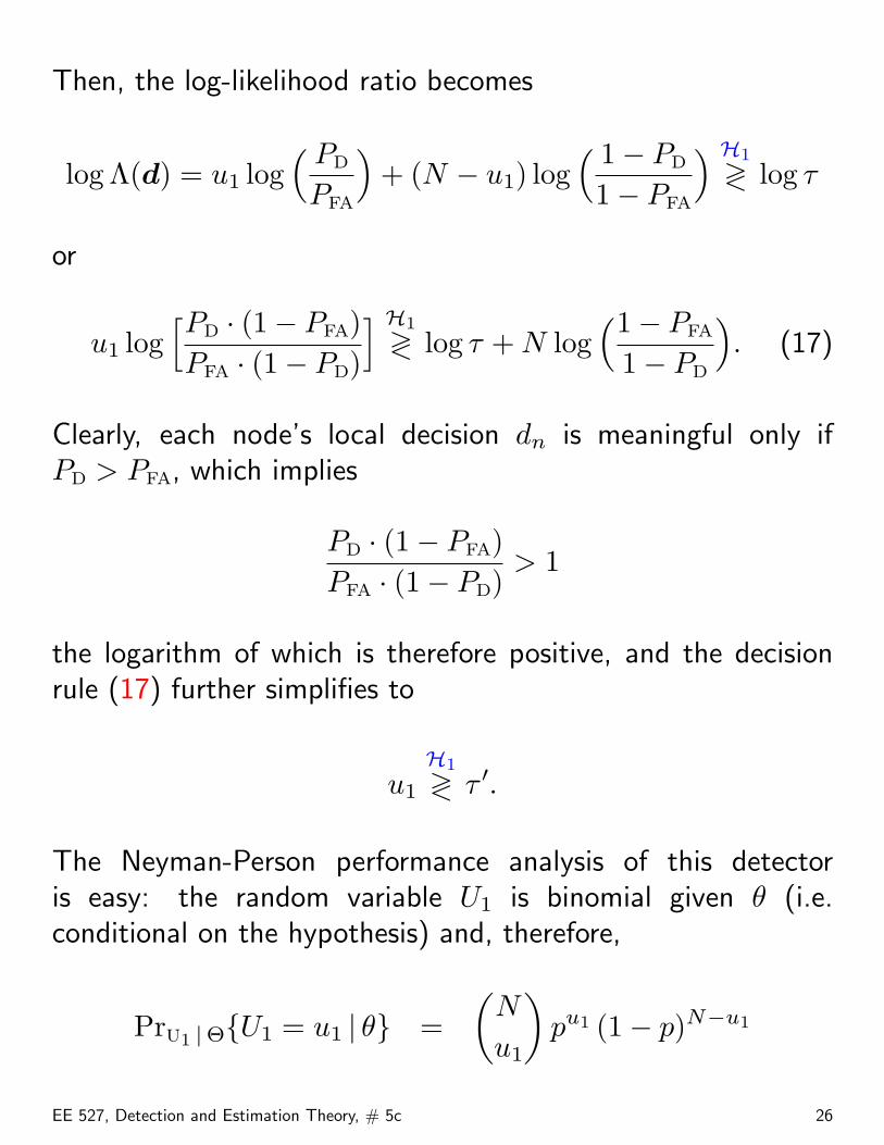
Then, the log-likelihood ratio becomes

log Λ(d) = u1 log( PD

PFA

)+ (N − u1) log

( 1− PD

1− PFA

) H1

≷ log τ

or

u1 log[PD · (1− PFA)PFA · (1− PD)

] H1

≷ log τ + N log(1− PFA

1− PD

). (17)

Clearly, each node’s local decision dn is meaningful only ifPD > PFA, which implies

PD · (1− PFA)PFA · (1− PD)

> 1

the logarithm of which is therefore positive, and the decisionrule (17) further simplifies to

u1

H1

≷ τ ′.

The Neyman-Person performance analysis of this detectoris easy: the random variable U1 is binomial given θ (i.e.conditional on the hypothesis) and, therefore,

PrU1 |Θ{U1 = u1 | θ} =(

N

u1

)pu1 (1− p)N−u1


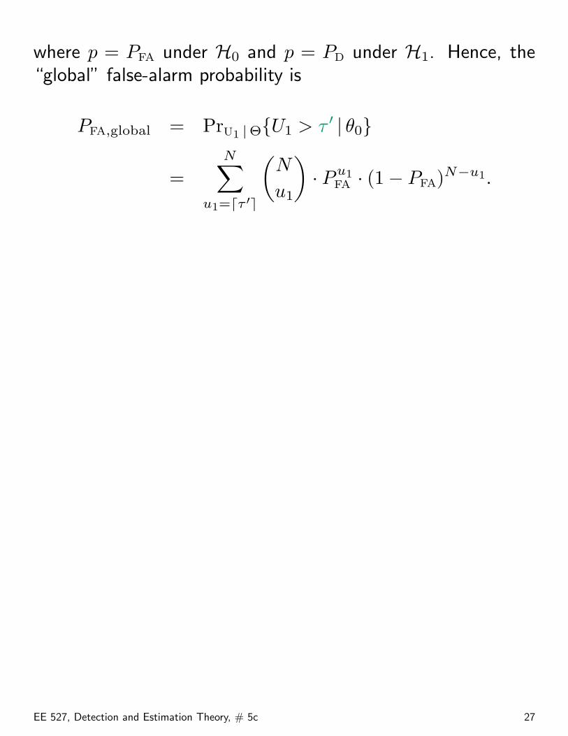
where p = PFA under H0 and p = PD under H1. Hence, the“global” false-alarm probability is

PFA,global = PrU1 |Θ{U1 > τ ′ | θ0}

=N∑

u1=dτ ′e

(N

u1

)· Pu1

FA · (1− PFA)N−u1.


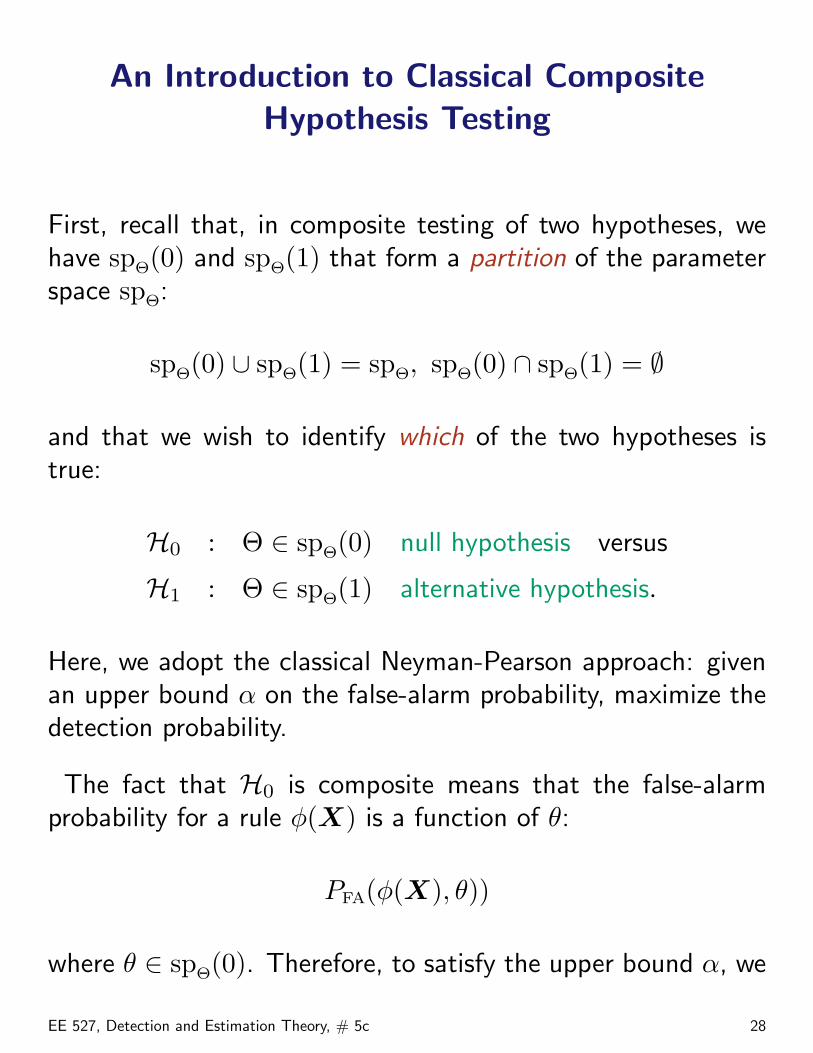
An Introduction to Classical CompositeHypothesis Testing

First, recall that, in composite testing of two hypotheses, wehave spΘ(0) and spΘ(1) that form a partition of the parameterspace spΘ:

spΘ(0) ∪ spΘ(1) = spΘ, spΘ(0) ∩ spΘ(1) = ∅

and that we wish to identify which of the two hypotheses istrue:

H0 : Θ ∈ spΘ(0) null hypothesis versus

H1 : Θ ∈ spΘ(1) alternative hypothesis.

Here, we adopt the classical Neyman-Pearson approach: givenan upper bound α on the false-alarm probability, maximize thedetection probability.

The fact that H0 is composite means that the false-alarmprobability for a rule φ(X) is a function of θ:

PFA(φ(X), θ))

where θ ∈ spΘ(0). Therefore, to satisfy the upper bound α, we


consider all tests φ(X) such that

maxθ∈spΘ(0)

PFA(φ(X), θ)) ≤ α. (18)

In this context,max

θ∈spΘ(0)PFA(φ(X), θ) (19)

is typically referred to as the size of the test φ(X). Therefore,the condition (18) states that we focus on tests whose size isupper-bounded by α.

Definition. Among all tests φ(X) whose size is upper-bounded by α [i.e. (18) holds], we say that φUMP(X) is auniformly most powerful (UMP) test if it satisfies

PD(φUMP(X), θ) ≥ PD(φ(X), θ)

for all θ ∈ spΘ(1).

This is a very strong statement and very few hypothesis-testingproblems have UMP tests. Note that Neyman-Pearson testsfor simple hypotheses are UMP.

Hence, to find an UMP test for composite hypotheses, weneed to first write a likelihood ratio for the simple hypothesistest with spΘ(0) = {θ0}, spΘ(1) = {θ1}, and spΘ = {θ0, θ1}and then transform this likelihood ratio in such a way thatunknown quantities (e.g. θ0 and θ1) disappear from the teststatistic.


(1) If such a transformation can be found, there is hope thata UMP test exists.

(2) However, we still need to figure out how to set a decisionthreshold (τ , say) such that the upper bound (18) is satisfied.


Example 1: Detecting a Positive DC Level inAWGN (versus zero DC level)

Consider the following composite hypothesis-testing problem:

H0 : θ = 0 i.e. θ ∈ spΘ(0) = {0} versus

H1 : θ > 0 i.e. θ ∈ spΘ(1) = (0,+∞)

where the measurements X[0], X[1], . . . , X[N − 1] areconditionally independent, identically distributed (i.i.d.) givenΘ = θ, modeled as

{X[n] |Θ = θ} = θ + W [n] n = 0, 1, . . . , N − 1

with W [n] a zero-mean white Gaussian noise with knownvariance σ2, i.e.

W [n] ∼ N (0, σ2)implying

fX |Θ(x | θ) =1√

(2 π σ2)N·exp

[− 1

2 σ2

N−1∑n=0

(x[n]−θ)2]

(20)

where x = [x[0], x[1], . . . , x[N − 1]]T . A sufficient statistic forθ is

x =1N

N∑n=1

x[n].


Now, find the pdf of x given Θ = θ:

fX |Θ(x | θ) = N (x | θ, σ2/N). (21)

We start by writing the classical Neyman-Pearson test for thesimple hypotheses with spsimple

Θ (0) = {0} and spsimpleΘ (1) =

{θ1}, θ1 ∈ (0,+∞):

fX |Θ(x | θ1)fX |Θ(x | 0)

=(2 π σ2/N)−1/2 · exp[− 1

2 σ2/N(x− θ1)2]

(2 π σ2/N)−1/2 · exp[− 12 σ2/N

(x)2]

H1

≷ λ.

Taking log etc. leads to

θ1 xH1

≷ η.

Since we know that θ1 > 0, we can divide both sides of theabove expression by θ1 and accept H1 if

φ(x) : xH1

≷ τ.

Hence, we transformed our likelihood ratio in such a way thatθ1 disappears from the test statistic, i.e. we accomplished (1)above.

Now, on to (2). How to determine the threshold τ such thatthe upper bound (18) is satisfied? Based on (25), we know:

fX |Θ(x | 0) = N (x | 0, σ2/N)


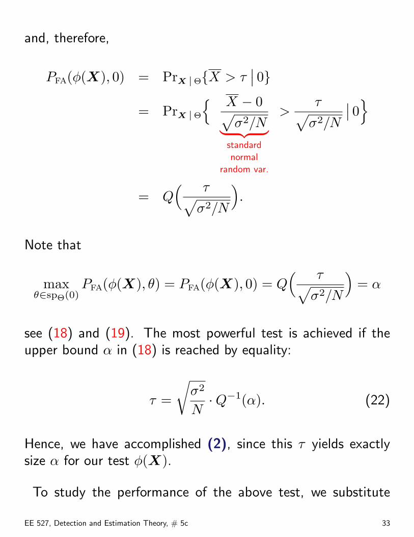
and, therefore,

PFA(φ(X), 0) = PrX |Θ{X > τ∣∣ 0}

= PrX |Θ

{ X − 0√σ2/N︸︷︷︸

standardnormal

random var.

>τ√

σ2/N

∣∣ 0}

= Q( τ√

σ2/N

).

Note that

maxθ∈spΘ(0)

PFA(φ(X), θ) = PFA(φ(X), 0) = Q( τ√

σ2/N

)= α

see (18) and (19). The most powerful test is achieved if theupper bound α in (18) is reached by equality:

τ =

√σ2

N·Q−1(α). (22)

Hence, we have accomplished (2), since this τ yields exactlysize α for our test φ(X).

To study the performance of the above test, we substitute


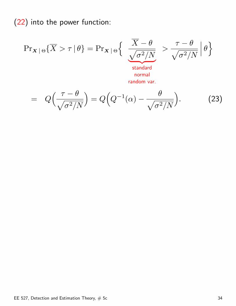
(22) into the power function:

PrX |Θ{X > τ | θ} = PrX |Θ

{ X − θ√σ2/N︸︷︷︸

standardnormal

random var.

>τ − θ√σ2/N

∣∣∣ θ}

= Q( τ − θ√

σ2/N

)= Q

(Q−1(α)− θ√

σ2/N

). (23)


Example 2: Detecting a Positive DC Level inAWGN (versus nonnegative DC level)

Consider the following composite hypothesis-testing problem:

H0 : θ ≤ 0 i.e. θ ∈ spΘ(0) = (−∞, 0] versus

H1 : θ > 0 i.e. θ ∈ spΘ(1) = (0,+∞)

where the measurements X[0], X[1], . . . , X[N − 1] areconditionally i.i.d. given Θ = θ, modeled as

{X[n] |Θ = θ} = θ + W [n] n = 0, 1, . . . , N − 1

with W [n] a zero-mean white Gaussian noise with knownvariance σ2, i.e.

W [n] ∼ N (0, σ2)implying

fX |Θ(x | θ) =1√

(2 π σ2)N·exp

[− 1

2 σ2

N−1∑n=0

(x[n]−θ)2]

(24)

where x = [x[0], x[1], . . . , x[N − 1]]T . A sufficient statistic forθ is

x =1N

N∑n=1

x[n].


andfX |Θ(x | θ) = N (x | θ, σ2/N). (25)

We start by writing the classical Neyman-Pearson test for thesimple hypotheses with spsimple

Θ (0) = {θ0} and spsimpleΘ (1) =

{θ1}, where θ0 ∈ (−∞, 0] and θ1 ∈ (0,+∞), implying

fX |Θ(x | θ1)fX |Θ(x | θ0)

=(2 π σ2/N)−1/2 · exp[− 1

2 σ2/N(x− θ1)2]

(2 π σ2/N)−1/2 · exp[− 12 σ2/N

(x− θ0)2]

H1

≷ λ

andθ0 < θ1.

Taking log etc. leads to

(θ1 − θ0) xH1

≷ η

and, since θ0 < θ1, to

φ(x) : xH1

≷ τ.

Hence, we transformed our likelihood ratio in such a way thatθ0 and θ1 disappear from the test statistic, i.e. we accomplished(1) above.

The power function of this test is

PrX |Θ{X > τ | θ} = PrX |Θ

{X − θ

σ/√

N>

τ − θ

σ/√

N

∣∣∣ θ} = Q( τ − θ

σ/√

N

)EE 527, Detection and Estimation Theory, # 5c 36

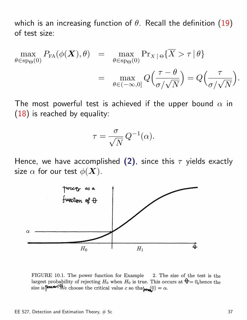
which is an increasing function of θ. Recall the definition (19)of test size:

maxθ∈spΘ(0)

PFA(φ(X), θ) = maxθ∈spΘ(0)

PrX |Θ{X > τ | θ}

= maxθ∈(−∞,0]

Q( τ − θ

σ/√

N

)= Q

( τ

σ/√

N

).

The most powerful test is achieved if the upper bound α in(18) is reached by equality:

τ =σ√N

Q−1(α).

Hence, we have accomplished (2), since this τ yields exactlysize α for our test φ(X).


Example 3: Detecting a Completely UnknownDC Level in AWGN

Consider now the composite hypothesis-testing problem:

H0 : θ = 0 i.e. θ ∈ spΘ(0) = {0} versus

H1 : θ 6= 0 i.e. θ ∈ spΘ(1) = (−∞,+∞)\{0}

where the measurements X[0], X[1], . . . , X[N − 1] areconditionally i.i.d. given Θ = θ, following

fX |Θ(x | θ) =1√

(2 π σ2)N· exp

[− 1

2 σ2

N−1∑n=0

(x[n]− θ)2]

and x = [x[0], x[1], . . . , x[N − 1]]T . A sufficient statistic for θ

is x = 1N

∑Nn=1 x[n] and the pdf of x given Θ = θ is

fX |Θ(x | θ) = N (x | θ, σ2/N). (26)

We start by writing the classical Neyman-Pearson test for thesimple hypotheses with spΘ(0) = {0} and spΘ(1) = {θ1 6= 0}:

θ1 x > η.

We cannot accomplish (1), since θ1 cannot be removed fromthe test statistic; therefore, UMP test does not exist for theabove problem.


Monotone Likelihood-ratio Criterion

Consider a scalar parameter θ. We say that

fX |Θ(x |θ)

belongs to the monotone likelihood ratio (MLR) family if thepdfs (or pmfs) from this family

• satisfy the identifiability condition for θ (i.e. these pdfs aredistinct for different values of θ) and

• there is a scalar statistic T (x) such that, for θ0 < θ1, thelikelihood ratio

Λ(x ; θ0, θ1) =fX |Θ(x | θ1)fX |Θ(x | θ0)

is a monotonically increasing function of T (x).

If fX |Θ(x |θ) belongs to the MLR family, then use the followingtest:

φλ(x) ={

1, for T (x) ≥ λ,0, for T (x) < λ


and set

α = PFA(φ(X), θ0) = PrX |Θ{T (X) ≥ λ | θ0} (27)

e.g. use this condition to find the threshold λ.

This test has the following properties:

(i) With α given by (27), φλ(x) is UMP test of size α fortesting

H0 : θ > θ0 versus

H1 : θ ≤ θ0.

(ii) For each λ, the power function

PrX |Θ{T (X) ≥ λ | θ} (28)

is a monotonically increasing function of θ.

Note: Consider the one-parameter exponential family

fX |Θ(x | θ) = h(x) exp[η(θ) T (x)−B(θ)]. (29)

Then, if η(θ) is a monotonically increasing function of θ, theclass of pdfs (pmfs) (29) satisfies the MLR conditions.


Example: Detection for Exponential RandomVariables

Consider conditionally i.i.d. measurements X[0], X[1], . . . , X[N−1] given the parameter θ > 0, following the exponential pdf:

fX |Θ(x[n] | θ) = Expon(x[n] | 1/θ)

=1θ

exp(−θ−1 x[n]) i(0,+∞)(x[n]).

The likelihood function of θ for all observations x =[x[0], x[1], . . . , x[N − 1]]T is

fX |Θ(x | θ) =1

θNexp[−θ−1 T (x)]

N−1∏n=0

i(0,+∞)(x[n])

where

T (x) =N−1∑n=0

x[n].

Since fX |Θ(x | θ) belongs to the one-parameter exponentialfamily (29) and η(θ) = −θ−1 is a monotonically increasingfunction of θ. Therefore, the test

φλ(x) ={

1, for T (x) ≥ λ,0, for T (x) < λ


is UMP for testing

H0 : θ > θ0 versus

H1 : θ ≤ θ0.

The sum of i.i.d. exponential random variables follows theErlang pdf (which is a special case of the gamma pdf):

fT |Θ(T | θ) =1

θN

TN−1

(N − 1)!exp(−T/θ) i(0,+∞)(T )

= Gamma(T |N, θ−1).

Therefore, the size of the test can be written as

α = PrX |Θ{T (X) ≥ λ | θ0}

=1

θN0

∫ +∞

λ

tN−1

(N − 1)!exp(−t/θ0) dt

=[1 +

λ

θ0+ · · ·+ 1

(N − 1)!( λ

θ0

)N−1]

exp(−λ/θ0)

where the integral is evaluated using integration by parts. ForN = 1, we have

λ = θ0 ln(1/α).


Generalized Likelihood Ratio (GLR) Test

Recall again that, in composite testing of two hypotheses, wehave spΘ(0) and spΘ(1) that form a partition of the parameterspace spΘ:

spΘ(0) ∪ spΘ(1) = spΘ, spΘ(0) ∩ spΘ(1) = ∅

and that we wish to identify which of the two hypotheses istrue:

H0 : θ ∈ spΘ(0) null hypothesis versus

H1 : θ ∈ spΘ(1) alternative hypothesis.

In GLR tests, we replace the unknown parameters by theirmaximum-likelihood (ML) estimates under the two hypotheses.Hence, accept H1 if

ΛGLR(x) =maxθ∈spΘ(1) fX |Θ(x | θ)maxθ∈spΘ(0) fX |Θ(x | θ)

> τ.

This test has no UMP optimality properties, but often workswell in practice.


Example: Detecting a Completely UnknownDC Level in AWGN

Consider again the composite hypothesis-testing problem fromp. 38:

H0 : θ = 0 i.e. θ ∈ spΘ(0) = {0} versus

H1 : θ 6= 0 i.e. θ ∈ spΘ(1) = (−∞,+∞)\{0}

where the measurements X[0], X[1], . . . , X[N − 1] areconditionally i.i.d. given Θ = θ, following

fX |Θ(x | θ) =1√

(2 π σ2)N· exp

[− 1

2 σ2

N−1∑n=0

(x[n]− θ)2]

and x = [x[0], x[1], . . . , x[N − 1]]T . A sufficient statistic for θ

is x = 1N

∑Nn=1 x[n] and the pdf of x given Θ = θ is

fX |Θ(x | θ) = N (x | θ, σ2/N).

Our GLR test accepts H1 if

ΛGLR(x) =maxθ∈spΘ(1) fX |Θ(x | θ)

fX |Θ(x | 0)> τ.

Now,x = arg max

θ∈spΘ(1)fX |Θ(x | θ)


and

fX |Θ(x | 0) = N (x | 0, σ2/N)

=1√

2 π σ2/Nexp

(− 1

2

x2

σ2/N

)fX |Θ(x |x) = N (x | 0, σ2/N) =

1√2 π σ2/N

yielding

lnΛGLR(x) =N x2

2 σ2.

Therefore, we accept H1 if

(x)2 > γ

or|x| > η.

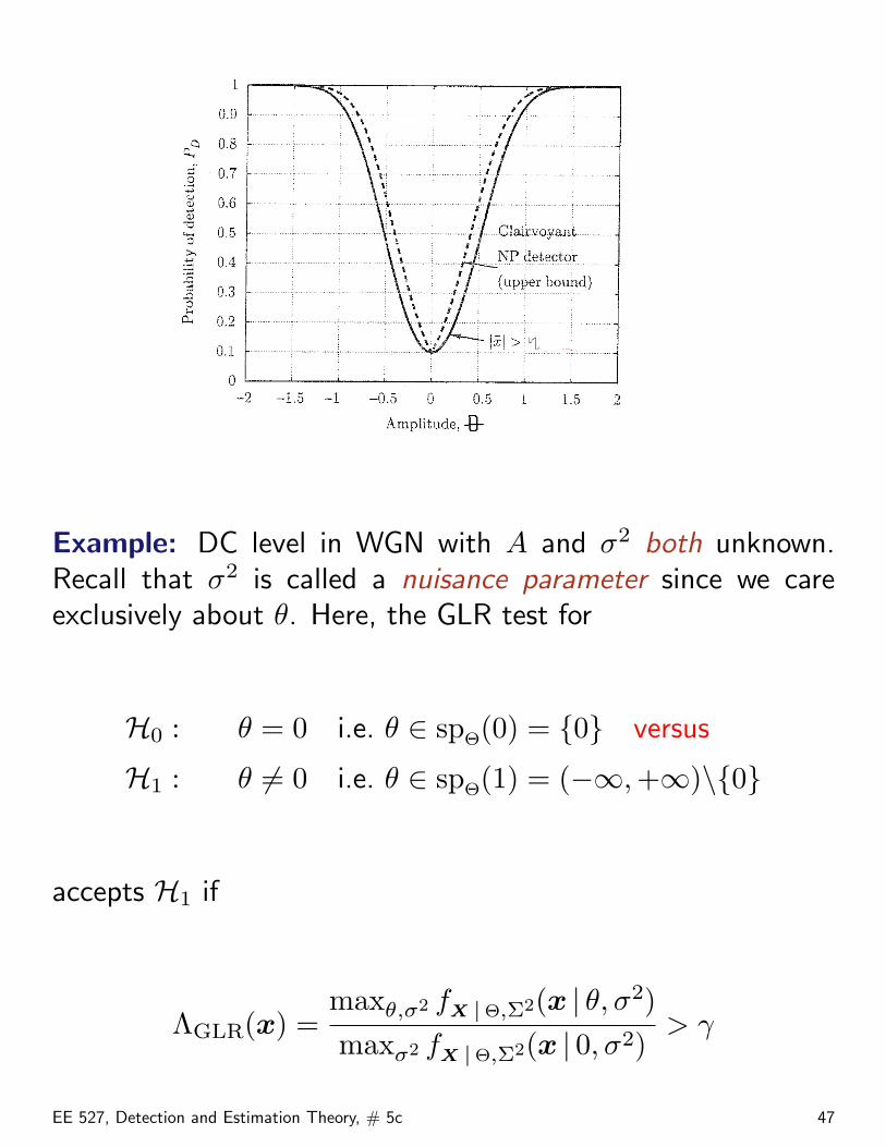
We compare this detector with the (not realizable, also calledclairvoyant) UMP detector that assumes the knowledge of thesign of θ under H1. Assuming that the sign of θ under H1 isknown, we can construct the UMP detector, whose ROC curveis given by

PD = Q(Q−1(PFA)− d)where d =

√N θ2/σ2 and θ is the value of the parameter

under H1; see (23) for the case where θ > 0 under H1. Allother detectors have PD below this upper bound.


GLR test: Decide H1 if |x| > η. To make sure that the GLRtest is implementable, we must be able to specify a threshold ηso that the false-alarm probability is upper-bounded by a givensize α. This is possible in our example:

PFA(φ(x), 0) = PrX |Θ{|X| > η | 0} see (26)

symmetry= 2 PrX |Θ{X > η | 0} = 2Q(η/

√σ2/N)

PD(φ(x), θ) = PrX |Θ{|X| > η | θ} see (26)

= PrX |Θ{X > η | θ}+ PrX |Θ{X < −η | θ}

= Q( η − θ√

σ2/N

)+ Q

( η + θ√σ2/N

)= Q

(Q−1(α/2)− θ√

σ2/N

)+Q(Q−1(α/2) +

θ√σ2/N

).

In this case, GLR test is only slightly worse than the clairvoyantdetector (Figure 6.4 in Kay-II):


Example: DC level in WGN with A and σ2 both unknown.Recall that σ2 is called a nuisance parameter since we careexclusively about θ. Here, the GLR test for

H0 : θ = 0 i.e. θ ∈ spΘ(0) = {0} versus

H1 : θ 6= 0 i.e. θ ∈ spΘ(1) = (−∞,+∞)\{0}

accepts H1 if

ΛGLR(x) =maxθ,σ2 fX |Θ,Σ2(x | θ, σ2)maxσ2 fX |Θ,Σ2(x | 0, σ2)

> γ


where

fX |Θ,Σ2(x | θ, σ2) =1√

(2 π σ2)N·exp

[− 1

2 σ2

N−1∑n=0

(x[n]−θ)2].

(30)Here,

maxθ,σ2

fX |Θ,Σ2(x | θ, σ2) =1

[2π σ̂21(x)]N/2

· e−N/2

maxσ2

fX |Θ,Σ2(x | 0, σ2) =1

[2π σ̂20(x)]N/2

· e−N/2

where

σ̂20(x) =

1N

N∑n=1

x2[n]

σ̂21(x) =

1N

N∑n=1

(x[n]− x)2.

Hence,

ΛGLR(x) =(

σ̂20(x)

σ̂21(x)

)N/2

i.e. GLR test fits data with the “best” DC-level signal θ̂ML = x,finds the residual variance estimate σ̂2

1, and compares thisestimate with the variance estimate σ̂2

0 under the null case (i.e.


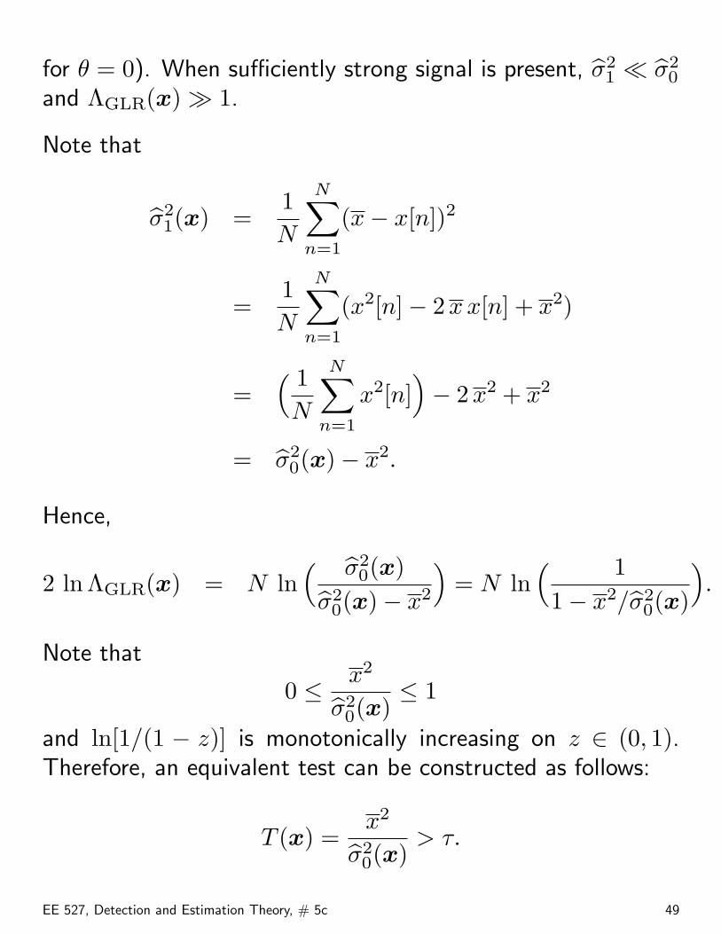
for θ = 0). When sufficiently strong signal is present, σ̂21 � σ̂2

0

and ΛGLR(x) � 1.

Note that

σ̂21(x) =

1N

N∑n=1

(x− x[n])2

=1N

N∑n=1

(x2[n]− 2 xx[n] + x2)

=( 1N

N∑n=1

x2[n])− 2 x2 + x2

= σ̂20(x)− x2.

Hence,

2 lnΛGLR(x) = N ln( σ̂2

0(x)σ̂2

0(x)− x2

)= N ln

( 11− x2/σ̂2

0(x)

).

Note that

0 ≤ x2

σ̂20(x)

≤ 1

and ln[1/(1 − z)] is monotonically increasing on z ∈ (0, 1).Therefore, an equivalent test can be constructed as follows:

T (x) =x2

σ̂20(x)

> τ.


The pdf of T (X) given θ = 0 does not depend on σ2 and,therefore, GLR test can be implemented, i.e. it is CFAR.

Definition. A test is constant false alarm rate (CFAR) if wecan find a threshold that yields a test whose size is equal to α.

In other words, we should be able to set the thresholdindependently of the unknown parameters, i.e. the distributionof the test statistic under H0 does not depend on the unknownparameters.


Neyman-Pearson test for simple binary hypotheses, …namrata/EE527_Spring08/l5c_2.pdf · Outline:...

Documents

Transcript of Neyman-Pearson test for simple binary hypotheses, …namrata/EE527_Spring08/l5c_2.pdf · Outline:...