New Tests of Forecast Optimality Across Multiple Horizons

New Tests of Forecast Optimality Across Multiple Horizons∗

Andrew J. Patton

Duke University

Allan Timmermann

University of California, San Diego

March 26, 2010

Preliminary and incomplete.

Abstract

We propose new joint tests of forecast optimality that exploit information contained in multi-horizon

forecasts. In addition to implying zero bias and zero autocorrelation in forecast errors, we show that forecast

optimality under squared error loss also implies testable restrictions on second moments of the data ordered

across forecast horizons. In particular, the variance of the forecast error should be increasing in the horizon;

the variance of the forecast itself should be decreasing in the horizon; and the variance of forecast revisions

should be bounded by twice the covariance of revisions with the target variable. These bounds on second

moments can be restated as inequality constraints in a regression framework and tested using the approach

of Wolak (1989). Moreover, some of the proposed tests can be conducted without the need for data on the

target variable, which is particularly useful in the presence of large measurement errors. We also propose a

new univariate optimal revision test that constrains the coeffi cients in a regression of the target variable on

the long-horizon forecast and the sequence of interim forecast revisions. The size and power of the new tests

are compared with those of extant tests through Monte Carlo simulations. An empirical application to the

Federal Reserve’s Greenbook forecasts is used to illustrate the tests.

Keywords: Forecast optimality, real-time data, variance bounds, survey forecasts, forecast horizon.

J.E.L. Codes: C53, C22, C52.

∗We thank Tim Bollerslev and Ken West as well as seminar participants at Duke, UCSD, EC2 conference on

real-time econometrics (December, 2009), and the 6th forecasting symposium at the ECB.

1 Introduction

Forecasts recorded at multiple horizons, for example from one to several quarters into the future,

are becoming increasingly common in empirical practice. For example, the surveys conducted by

the Philadelphia Federal Reserve (Survey of Professional Forecasters), Consensus Economics or

Blue Chip and the forecasts produced by the IMF (World Economic Outlook), the Congressional

Budget offi ce, the Bank of England and the Board of the Federal Reserve all cover several hori-

zons. Similarly, econometric models are commonly used to generate multi-horizon forecasts, see,

e.g., Faust and Wright (2009), Marcellino, Stock and Watson (2006), and Clements (1997). With

the availability of such multi-horizon forecasts, there is a growing need for tests of optimality to

exploit the information in the complete “term structure”of forecasts recorded across all horizons.

By simultaneously exploiting information across several horizons, rather than focusing separately

on individual horizons, multi-horizon forecast tests offer the potential of drawing more powerful

conclusions about the ability of forecasters to produce optimal forecasts. This paper derives a

number of novel and simple implications of forecast optimality and compares tests based on these

implications with extant tests.

A well-known implication of forecast optimality is that, under squared error loss, the mean

squared forecast error should be a non-decreasing function of the forecast horizon, see, e.g., Diebold

(2001) and Patton and Timmermann (2007a). A similar property holds for the forecasts themselves:

Internal consistency of a sequence of optimal forecasts implies that the variance of the forecasts

should be a non-increasing function of the forecast horizon. Intuitively, this property holds because,

just as the variance of the realized value must be (weakly) greater than the variance of its conditional

expectation, the variance of the expectation conditional on a large information set (corresponding

to a short horizon) must exceed that of the expectation conditional on a smaller information set

(corresponding to a long horizon). It is also possible to show that optimal updating of forecasts

implies that the variance of the forecast revision should exceed twice the covariance between the

forecast revision and the actual value. It is uncommon to test such variance bounds in empirical

practice, in part due to the diffi culty in setting up joint tests of these bounds. We suggest and

illustrate testing these monotonicity properties via tests of inequality contraints using the methods

Gourieroux et al. (1982) and Wolak (1987, 1989).

Tests of forecast optimality have conventionally been based on comparing predicted and “re-

1

alized”values of the outcome variable. This severely constrains inference in some cases since, as

shown by Croushore (2006), Croushore and Stark (2001) and Corradi, Fernandez and Swanson

(2009), revisions to macroeconomic variables can be very considerable. This raises questions that

can be diffi cult to address such as “what are the forecasters trying to predict?”, i.e. first-release

data or final revisions. We show that variations on both the new and extant optimality tests can

be applied without the need for observations on the target variable. These tests are particularly

useful in situations where the target variable is not observed (such as for certain types of volatility

forecasts) or is measured with considerable noise (as in the case of output forecasts).

Conventional tests of forecast optimality regress the realized value of the predicted variable on

an intercept and the forecast for a single horizon and test the joint implication that the intercept and

slope coeffi cient are zero and one, respectively (Mincer and Zarnowitz (1969).) In the presence of

forecasts covering multiple horizons, we show that a complete test that imposes internal consistency

restrictions on the forecast revisions gives rise to a generalized effi ciency regression. Using a single

equation, this test is undertaken by regressing the realized value on an intercept, the long-horizon

forecast and the sequence of intermediate forecast revisions. A set of zero-one equality restrictions

on the intercept and slope coeffi cients are then tested. A key difference from the conventional

Mincer-Zarnowitz test is that the joint consistency of all forecasts at different horizons is tested by

this generalized regression.

Analysis of forecast optimality is usually predicated on covariance stationarity assumptions.

However, we show that the conventional assumption that the target variable and forecast are

(jointly) covariance stationary is not needed for some of our tests and can be relaxed provided that

forecasts for different horizons are lined up in “event time”, as studied by Nordhaus (1987) and

Clements (1997). In particular, we show that the second moment bounds continue to hold in the

presence of structural breaks in the variance of the innovation to the predicted variable. We present

a general family of data generating processes for which the variance bounds continue to hold.

To shed light on the statistical properties of the variance bound and regression-based tests of

forecast optimality, we undertake a set of Monte Carlo simulations. These simulations consider var-

ious scenarios with zero, low and high measurement error in the predicted variable and deviations

from forecast optimality in a variety different directions. We find that the covariance bound and the

single-equation test of joint forecast consistency have good power and size properties. Specifically,

they are generally better than conventional Mincer-Zarnowitz tests conducted for individual hori-

2

zons which either tend to be conservative−if a Bonferroni bound is used to summarize the evidence

across multiple horizons−or suffer from substantial size distortions, if the multi-horizon regressions

are estimated as a system. Our simulations suggest that the various bounds and regression tests

have complementary properties in the sense that they have power in different directions and so can

identify different types of suboptimal behavior among forecasters.

An empirical application to Greenbook forecasts of GDP growth, changes to the GDP deflator

and consumer price inflation confirms the findings from the simulations. In particular, we find that

conventional regression tests often fail to reject the null of forecast optimality. In contrast, the new

variance-bounds tests and single equation multi-horizon tests have better power and are able to

identify deviations from forecast optimality.

The outline of the paper is as follows. Section 2 presents some novel implications of optimality of

forecasts across multiple horizons, and descibes hypothesis tests associated with these implications.

Section 3 considers regression-based tests of forecast optimality and Section 4 discusses the role of

stationarity for fixed-event forecasts. Section 5 presents the results from the Monte Carlo study,

while Section 6 provides an empirical application to Federal Reserve Greenbook forecasts. Section

7 concludes.

2 Variance Bounds Tests

In this section we derive variance and covariance bounds that can be used to test the optimality

of a sequence of forecasts recorded at different horizons. These are presented as corollaries to the

well-known theorem that the optimal forecast under quadratic loss is the conditional mean. The

proofs of these corollaries are straightforward, and are collected in the Appendix.

2.1 Assumptions and background

Consider a univariate time series, Y ≡ {Yt; t = 1, 2, ...}, and suppose that forecasts of this variable

are recorded at different points in time, t = 1, ..., T and at different horizons, h = h1, ..., hH .

Forecasts of Yt made h periods previously will be denoted as Yt|t−h and is thus conditioned on

the available information set at time t − h, Ft−h, which is taken to be the σ-field generated by{Zt−h−k; k ≥ 0

}, where Zt−h is a vector of predictor variables capturing elements in the forecaster’s

information set at time t− h. Note that the target variable, Yt, may or may not be an element of

3

Zt, depending on whether this variable is observable to the forecaster or not. Forecast errors are

given by et|t−h = Yt− Yt|t−h. We consider an (H × 1) vector of multi-horizon forecasts for horizons

h1 < h2 < · · · < hH , with generic long and short horizons denoted by hL and hS (hL > hS).

Note that the forecast horizons, hi, can be positive, zero or negative, corresponding to forecasting,

nowcasting or backcasting, and further note that we do not require the forecast horizons to be

equally spaced.

We consider tests of forecast optimality under the assumption that the forecaster has squared

error loss, and under that assumption we have the following well-known theorem, see Granger

(1969) for example.

Theorem 1 (Optimal forecast under MSE) Assume that the forecaster’s loss function is

L (y, y) = (y − y)2 and that the conditional mean of the target variable, E [Yt|Ft−h] is a.s. finite

for all t. Then

Y ∗t|t−h ≡ arg miny∈Y

E[(Yt − y)2 |Ft−h

]= E [Yt|Ft−h] (1)

where Y ⊆ R is the set of possible values for the forecast.

From this result it is simple to show that the associated forecast errors, e∗t|t−h = Yt − Y ∗t|t−h are

mean-zero and uncorrelated with any Zt−h ∈ Ft−h.We next describe a variety of forecast optimality

tests based on corollaries to this theorem.

Our analysis does not restrict the predicted “event”to be a single period outcome such as GDP

growth in 2011Q4. Instead the predicted outcome could be the cumulated GDP growth over some

period, say 20011Q1 through 2011Q4. Only the interpretation of the forecast horizon will change

in the latter situation, e.g. if the point of the forecast is 2011Q3, in which case part of the predicted

variable may be observed.

The tests proposed and studied in this paper take the forecasts as primitive, and if the forecasts

are generated by particular econometric models, rather than by a combination of modeling and

judgemental information, the estimation error embedded in those models is ignored. In the presence

of estimation error the results established here need not hold. In practice forecasters face parameter

uncertainty, model uncertainty and model instability issues and, as shown by West and McCracken

(1998), parameter estimation error can lead to substantial skews in unadjusted t−statistics. While

some of these effects can be addressed when comparing the relative precision of two forecasting

models evaluated at the pseudo-true probability limit of the model estimates (West (1996)) or when

4

comparing forecasting methods conditionally (Giacomini and White (2006)), it is not in general

possible to establish results for the absolute forecasting performance of a forecasting model. For

example, under recursive parameter estimation, forecast errors will generally be serially correlated

(Timmermann (1993)) and the mean squared forecast error may not be increasing in the forecast

horizon (Schmidt (1974), Clements and Hendry (1998)). Existing analytical results are very limited,

however, as they assume a particular model (e.g., an AR(1) specification), whereas in practice

forecasts from surveys and forecasts reported by central banks reflect considerable judgmental

information. We leave the important extension to incorporate estimation error to future research.

Some of the results derived below will make use of a standard covariance stationarity assumtion:

Assumption S1: The target variable, Yt, is generated by a covariance stationary process.

2.2 Monotonicity of mean squared errors

From forecast optimality under squared-error loss, (1), it follows that, for any Yt|t−h ∈ Ft−h,

Et−h

[(Yt − Y ∗t|t−h

)2]≤ Et−h

[(Yt − Yt|t−h

)2].

In particular, the optimal forecast at time t−hS must be at least as good as the forecast associated

with a longer horizon, hL:

Et−h

[(Yt − Y ∗t|t−hS

)2]≤ Et−h

[(Yt − Y ∗t|t−hL

)2].

This leads us to the first corollary to Theorem 1 (all proofs are contained in the Appendix):

Corollary 1 Under the assumptions of Theorem 1 and S1, it follows that

MSE (hS) ≡ E[(Yt − Y ∗t|t−hS

)2]≤ E


)2]≡MSE (hL) for any hS < hL.

Given a set of forecasts available at horizons h1 ≤ h2.... ≤ hH , it follows that the mean squared

error (MSE) associated with an optimal forecast, e∗t|t−h ≡ Yt − Y∗t|t−h, is a non-decreasing function

of the forecast horizon:

E[e∗2t|t−h1

]≤ E

[e∗2t|t−h2

]≤ ... ≤ E

[e∗2t|t−hH

]→ V [Yt] as hH →∞, (2)

The inequalities are strict if more forecast-relevant information becomes available as the forecast

horizon shrinks to zero.1 This property is well-known and is discussed by, e.g., Diebold (2001) and1For example, for a non-degenerate AR(1) process the MSEs will strictly increase with the forecast horizon, while

for an MA(1) the inequality will be strict only for h = 1 vs. h = 2, while for longer horizons the MSEs will be equal.

5

Patton and Timmermann (2007a).

Example 1: To illustrate a violation of this property, consider the case of a “lazy”forecaster,

who, in constructing a short-horizon forecast, Yt|t−hS , does not update his long-horizon forecast,

Yt|t−hL , with relevant information, and hides this lack of updating by adding a small amount of

zero-mean, independent noise to the long-horizon forecast. In that case:

Yt|t−hS = Yt|t−hL + ut−hS , ut−hS ⊥ Yt|t−hL , ut−hS ⊥ Yt. (3)

We then have

V[et|t−hS

]= V

[Yt − Yt|t−hL − ut−hS

]= V

[et|t−hL − ut−hS

]= V

[et|t−hL

]+V [ut−hS ] > V

[et|t−hL

].

Hence the short-horizon forecast generates a larger MSE than the long-horizon forecast, revealing

the sub-optimality of the short-horizon forecast.

2.3 Testing monotonicity in squared forecast errors

The results derived so far suggest testing forecast optimality via a test of the weak monotonicity in

the “term structure”of mean squared errors, (2), to use the terminology of Patton and Timmermann

(2008). This feature of rational forecasts is relatively widely known, but has generally not been

used to test forecast optimality. Capistran (2007) is the only paper we are aware of that exploits

this property to develop a test. His test is based on Bonferroni bounds, which are quite conservative

in this application. Here we advocate an alternative procedure for testing non-decreasing MSEs at

longer forecast horizons that is based on the inequalities in (2).

We consider ranking the MSE-values for a set of forecast horizons h = h1, h2, ..., hH . Denoting

the expected (population) value of the MSEs by µe = [µe1, ..., µeH ]′, with µej ≡ E[e2t|t−hj ], and

defining the associated MSE differentials as

∆ej ≡ µj − µj−1 = E

[e2t|t−hj

]− E

[e2t|t−hj−1

],

we can rewrite the inequalities in (2) as

∆ej ≥ 0, for j = h2, ..., hH . (4)

Following earlier work on multivariate inequality tests in regression models by Gourieroux, et

6

al. (1982), Wolak (1987, 1989) proposed testing (weak) monotonicity through the null hypothesis:

H0 : ∆e ≥ 0, (5)

vs. H1 : ∆e ∈ RH−1,

where the (H − 1)× 1 vector of MSE-differentials is given by ∆e ≡ [∆e2, ...,∆

eH ]′. In contrast, ∆e

is unconstrained under the alternative. Tests can be based on the sample analogs ∆ej = µj − µj−1

for µj ≡ 1T

∑Tt=1 e

2t|t−hj . Wolak (1987, 1989) derives a test statistic whose distribution under the

null is a weighted sum of chi-squared variables,∑H−1

i=1 ω(H − 1, i)χ2(i), where ω(H − 1, i) are the

weights and χ2(i) is a chi-squared variable with i degrees of freedom. Approximate critical values

for this test can be calculated through Monte Carlo simulation. For further description of this test

and other approaches to testing multivariate inequalities, see Patton and Timmermann (2009).

2.4 Monotonicity of mean squared forecasts

We now present a novel implication of forecast optimality that can be tested when data on the

target variable is not available or not reliable. Recall that, under optimality, Et−h[e∗t|t−h

]= 0

which implies that Cov[Y ∗t|t−h, e

∗t|t−h

]= 0. Thus we obtain the following corollary:

Corollary 2 Under the assumptions of Theorem 1 and S1, we have V [Yt] = V[Y ∗t|t−h

]+E

[e∗2t|t−h

].

From Corollary 1 we have E[e∗2t|t−hS

]≤ E

[e∗2t|t−hL

]for any hS < hL, which then yields

V[Y ∗t|t−hS

]≥ V

[Y ∗t|t−hL

]for any hS < hL.

Further, since E[Y ∗t|t−h

]= E [Yt] , we also obtain an inequality on the mean-squared forecasts:

E[Y ∗2t|t−hS

]≥ E

[Y ∗2t|t−hL

]for any hS < hL. (6)

This reveals that a weakly increasing pattern in MSE-values as the forecast horizon increases

implies a weakly decreasing pattern in the variance of the forecasts themselves. This simple result

provides the surprising implication that (one aspect of) forecast optimality may be tested without

the need for a measure of the target variable. A test of this implication can again be based on

Wolak’s (1989) approach by defining the vector ∆f ≡[∆f2 , ...,∆

fH

]′, where ∆f

j ≡ E[Y ∗2t|t−hj

]−

E[Y ∗2t|t−hj−1

]and testing the null hypothesis that differences in mean squared forecasts are weakly

7

negative for all forecast horizons:

H0 : ∆f ≤ 0, (7)

vs. H1 : ∆f ∈ RH−1.

It is worth pointing out some limitations to this type of test. Tests that do not rely on observing

the realized values of the target variable are tests of the internal consistency of the forecasts across

two or more horizons. For example, forecasts of an artificially-generated AR(p) process, independent

of the actual series but constructed in a theoretically optimal fashion, would not be identified as

suboptimal by this test.2

Example 2: Consider a scenario where all forecasts are contaminated with noise (due, e.g., to

estimation error) that is increasing in the forecast horizon:

Yt|t−hL = Y ∗t|t−hL + ut−hL , ut−hL ⊥ Yt|t−hL

Yt|t−hS = Y ∗t|t−hS + ut−hS , ut−hS ⊥(Yt|t−hL , Yt|t−hS , ut−hL

)V [ut−hL ] > V [ut−hS ] .

Define the forecast revision from time t− hL to t− hS as ηt|hS ,hL ≡ Y∗t|t−hS − Y

∗t|t−hL . Note that by

forecast optimality we have Cov[Y ∗t|t−hL , ηt|hS ,hL

]= 0, and so:

V[Yt|t−hS

]− V

[Yt|t−hL

]= V

[Y ∗t|t−hS

]+ V [ut−hS ]− V

[Y ∗t|t−hL

]− V [ut−hL ]

= V[Y ∗t|t−hL + ηt|hS ,hL

]+ V [ut−hS ]− V

[Y ∗t|t−hL

]− V [ut−hL ]

= V[ηt|hS ,hL

]+ V [ut−hS ]− V [ut−hL ]

< 0 if V [ut−hL ] > V[ηt|hS ,hL

]+ V [ut−hS ] .

Hence, if the contaminating noise in the long-horizon forecast is greater than the sum of the variance

of the optimal forecast revision and the variance of the short-horizon noise, the long-horizon forecast

will have greater variance than the short-horizon forecast, and a test based on (6) should detect

this.

Note that the violation of forecast optimality discussed in Example 1, with the short-horizon

forecast generated as the long-horizon forecast plus some independent noise, would not be detected

as sub-optimal by a test of the monotonicity of the mean-squared forecast. In this case the short-

horizon forecast would indeed be more volatile than the long-horizon forecast, consistent with2For tests of internal consistency across point forecasts and density forecasts, see Clements (2009).

8

optimality, and this test would not be able to detect that the source of this increased variation was

simply uninformative noise.

2.5 Monotonicity of covariance between the forecast and target variable

An implication of the weakly decreasing forecast variance property established in Corollary 2 is

that the covariance of the forecasts with the target variable should be decreasing in the forecast

horizon. To see this, note that

Cov[Y ∗t|t−h, Yt

]= Cov

[Y ∗t|t−h, Y

∗t|t−h + e∗t|t−h

]= V

[Y ∗t|t−h

].

Thus we obtain the following:

Corollary 3 Under the assumptions of Theorem 1 and S1, we obtain

Cov[Y ∗t|t−hS , Yt

]≥ Cov

[Y ∗t|t−hL , Yt

]for any hS < hL.

Further, since E[Y ∗t|t−h

]= E [Yt] , we also obtain:

E[Y ∗t|t−hSYt

]≥ E

[Y ∗t|t−hLYt

]for any hS < hL.

As for the above cases, this implication can again be tested using Wolak’s (1989) approach by

defining the vector ∆c ≡ [∆c2, ...,∆

cH ]′, where ∆c

j ≡ E[Y ∗t|t−hjYt

]−E

[Y ∗t|t−hj−1Yt

]and testing the

null hypothesis:

H0 : ∆c ≤ 0, (8)

vs. H1 : ∆c ∈ RH−1.

2.6 Monotonicity of mean squared forecast revisions

Monotonicity of mean squared forecasts also implies a monotonicity result for the mean squared

forecast revisions. Consider the following decomposition of the short-horizon forecast into the

long-horizon forecast plus the sum of forecast revisions:

Y ∗t|t−h1 = Y ∗t|t−hH +(Y ∗t|t−hH−1 − Y

∗t|t−hH

)+ ...+

(Y ∗t|t−h1 − Y

∗t|t−h2

)≡ Y ∗t|t−hH +

H−1∑j=1

ηt|hj ,hj+1 , (9)

9

where ηt|hS ,hL ≡ Y ∗t|t−hS − Y∗t|t−hL for hS < hL. Under optimality, Et−hL

[ηt|hS ,hL

]= 0 for all

hS < hL, so Cov[Y ∗t|t−hL , ηt|hS ,hL

]= 0, and

V[Y ∗t|t−h1 − Y

∗t|t−hH

]= V

H−1∑j=1

ηt|hj ,hj+1

=

H−1∑j=1

V[ηt|hj ,hj+1

],

V[Y ∗t|t−h1 − Y

∗t|t−hH−1

]=

H−2∑j=1

V[ηt|hj ,hj+1

]≤ V

[Y ∗t|t−h1 − Y

∗t|t−hH

]More generally, the following corollary to Theorem 1 holds:

Corollary 4 Denote the forecast revision between two dates as ηt|hS ,hL ≡ Y∗t|t−hS − Y

∗t|t−hL for any

hS < hL. Under the assumptions of Theorem 1 and S1, we have

V[ηt|hS ,hL

]≥ V

[ηt|hS ,hM

]for any hS < hM < hL.

Further, since E[ηt|hS ,hL

]= 0, we also obtain:

E[η2t|hS ,hL

]≥ E

[η2t|hS ,hM

]for any hS < hM < hL. (10)

Considering the forecast revisions between each horizon and the shortest horizon, this implies

that

V[ηt|h1,h2

]≤ V

[ηt|h1,h3

]≤ · · · ≤ V

[ηt|h1,hH

]. (11)

Again Wolak’s (1987, 1989) testing framework can be applied here: Define the vector of mean-

squared forecast revisions ∆η ≡[∆η3, ...,∆

ηH

]′, where ∆ηj ≡ E

[η2t|h1,hj

]− E

[η2t|1,hj−1

]= E

[(Y ∗t|t−h1 − Y

∗t|t−hj

)2]− E

[(Y ∗t|t−h1 − Y

∗t|t−hj−1

)2]. Then we can test the null hypothesis

that the differences in mean-squared forecast revisions are weakly positive for all forecast horizons:

H0 : ∆η ≥ 0, (12)

vs. H1 : ∆η ∈ RH−2.

Example 3: Consider forecasts with either “sticky”updating or, conversely, “overshooting”:

Yt|t−h = γY ∗t|t−h + (1− γ)Y ∗t|t−h−1, for h = 1, 2, ...,H.

“Sticky” forecasts correspond to γ ∈ [0, 1), while “overshooting” occurs when γ > 1. Moreover,

suppose the underlying data generating process is an AR(1), Yt = φYt−1 + εt, |φ| < 1, so Y ∗t|t−h =

10

φhYt−h. Then we have

ηt|t−h,t−h−1 = γ(Y ∗t|t−h − Y∗t|t−h−1) + (1− γ)(Y ∗t|t−h−1 − Y

∗t|t−h−2)

= γ(φhYt−h − φh+1Yt−h−1) + (1− γ)(φh+1Yt−h−1 − φh+2Yt−h−2)

= γφhεt−h + (1− γ)φh+1εt−h−1.

It follows that the variances of the one- and two-period forecast revisions are

V (ηt|1,2) =(γ2φ2 + (1− γ)2φ4

)σ2ε,

V (ηt|1,3) =(γ2φ2 + φ4 + (1− γ)2φ6

)σ2ε.

We can then have a violation of the inequality in (11), if

(1− γ)2 > 1 + (1− γ)2φ2.

There is clearly no violation if γ = 1 (full optimality) or if γ is close to one. However, if γ is far

from one, representing either very sticky forecasts (e.g., γ = 0.5) or overshooting (e.g., γ = 1.5).

2.7 Bounds on covariances of forecast revisions

Combining the inequalities contained in the above corollaries, it turns out that we can place an

upper bound on the variance of the forecast revision, as a function of the covariance of the revision

with the target variable. The intuition behind this bound is simple: if little relevant information

arrives between the updating points, then the variance of the forecast revisions must be low.

Corollary 5 Denote the forecast revision between two dates as ηt|hS ,hL ≡ Y∗t|t−hS − Y

∗t|t−hL for any

hS < hL. Under the assumptions of Theorem 1 and S1, we have

V[ηt|hS ,hL

]≤ 2Cov

[Yt, ηt|hS ,hL

]for any hS < hL.

Further, since E[ηt|hS ,hL

]= 0, we also obtain:

E[η2t|hS ,hL

]≤ 2E

[Ytηt|hS ,hL

]for any hS < hL. (13)

Note also that this result implies (as one would expect) that the covariance between the target

variable and the forecast revision must be positive; when forecasts are updated to reflect new

information, the change in the forecast should be positively correlated with the target variable.

11

The above bound can be tested by re-writing it as

E[2Ytηt|hS ,hL − η

2t|hS ,hL

]≥ 0. (14)

and forming the vector ∆b ≡[∆b2, ...,∆

bH

]′, where ∆b

j ≡ E[2Ytηt|hj ,hj−1 − η

2t|hj ,hj−1

], for j =

2, ...,H and then testing the null hypothesis that this variable is weakly positive for all forecast

horizons

H0 : ∆b ≥ 0

vs. H1 : ∆b ∈ RH−1.

Example 1, continued: Consider once again the case where the short-horizon forecast is

equal to the long-horizon forecast plus noise:

Yt|t−hS = Yt|t−hL + ut−hS , ut−hS ⊥ Yt|t−hL .

The difference between the variance of the forecast revision and twice the covariance of the revision

with the target variable (which is negative under forecast optimality) now equals the variance of

the noise:

V[ηt|hS ,hL

]− 2Cov

[Yt, ηt|hS ,hL

]= V

[Yt|t−hL + ut−hS − Yt|t−hL

]− 2Cov

[Yt, Yt|t−hL + ut−hS − Yt|t−hL

]= V [ut−hS ] > 0.

Here the bound is violated: The extra noise in the short-horizon forecast contributes to the variance

of the forecast revision without increasing the covariance of the revision with the target variable.

Example 2, continued: Consider again the case where all forecasts are contaminated with

noise, Yt|t−h = Yt|t−hL + ut|h, whose variance is increasing in the forecast horizon, V[ut|hL

]>

V[ut|hS

]. In this case we find:

V[ηt|hS ,hL

]− 2Cov

[Yt, ηt|hS ,hL

]= V

[ηt|hS ,hL + ut|hS − ut|hL

]− 2Cov

[Yt, ηt|hS ,hL + ut|hS − ut|hL

]=

{V[ηt|hS ,hL

]− 2Cov

[Yt, ηt|hS ,hL

]}+ V

[ut|hS

]+ V

[ut|hL

].

Under forecast optimality we know that the term in braces is negative, but if the sum of the short-

horizon and long-horizon noise is greater in absolute value than the term in braces, we will observe

a violation of the bound, and a test of this bound can be used to reject forecast optimality.

12

2.8 Variance bounds tests without data on the target variable

The “real time”macroeconomics literature has demonstrated the presence of large and prevalent

measurement errors affecting a variety of macroeconomic variables, see Croushore (2006), Croushore

and Stark (2001), Faust, Rogers and Wright (2005), and Corradi, Fernandez and Swanson (2009).

In such situations it is useful to have tests that do not require data on the target variable. Corollaries

2 and 4 presented two testable implications of forecast optimality that do not require data on the

target variable, and in this section we present further tests of multi-horizon forecast optimality that

can be employed when data on the target variable is not available or is not reliable.

The tests in this section exploit the fact that, under the null of forecast optimality, the short-

horizon forecast can be taken as a proxy for the target variable, from the stand-point of longer-

horizon forecasts, in the sense that the inequality results presented above all hold when the short-

horizon forecast is used in place of the target variable. Importantly, unlike standard cases, the

proxy in this case is smoother rather than noisier than the actual variable. This turns out to have

beneficial implications for the finite-sample performance of these tests when the measurement error

is sizeable or the predictive R2 of the forecasting model is low.

The result that corresponds to that in Corollary 1 is presented in Corollary 4. The corresponding

results for Corollaries 3 and 5 are presented below:

Corollary 6 Under the assumptions of Theorem 1 and S1 we obtain:

(a)

Cov[Y ∗t|t−hM , Y

∗t|t−hS

]≥ Cov

[Y ∗t|t−hL , Y

∗t|t−hS

], and (15)

E[Y ∗t|t−hM Y

∗t|t−hS

]≥ E

[Y ∗t|t−hL Y

∗t|t−hS

]for any hS < hM < hL

(b) Denote the forecast revision between two dates as ηt|h,k ≡ Y ∗t|t−h − Y∗t|t−k for any h < k.

Then

V[ηt|hM ,hL

]≤ 2Cov

[Y ∗t|t−hS , ηt|hM ,hL

], and (16)

E[η2t|hM ,hL

]≤ 2E

[Y ∗t|t−hSηt|hM ,hL

]for any hS < hM < hL.

As for Corollaries 3 and 5, an inevitable side-effect of testing forecast optimality without using

data on the target variable is that such a test only examines the internal consistency of the forecasts

across the different horizons; an internally consistent set of forecasts that are not optimal for a given

target variable will not be detected using such tests.

13

2.9 Illustration for an AR(1) process

This section illustrates the above results for the special case of an AR(1) process. Let:

Yt = φYt−1 + εt, |φ| < 1, (17)

where εt ∼WN(0, σ2ε), so σ2y = σ2ε/(1− φ2). Rewriting this as

Yt = φhYt−h +h−1∑i=0

φiεt−i,

we have Y ∗t|t−h = φhYt−h, and so e∗t|t−h =∑h−1

i=0 φiεt−i. From this it follows that, consistent with

Corollary 1,

V[e∗t|t−h

]= σ2ε

(1− φ2h

1− φ2

)≤ σ2ε

(1− φ2(h+1)

1− φ2

)= V

[e∗t|t−h−1

].

Moreover, consistent with Corollary 2 the variance of the forecast is increasing in h :

V[Y ∗t|t−h

]= φ2hσ2y ≥ φ2(h+1)σ2y = V

[Y ∗t|t−h−1

].

The covariance between the outcome and the h−period forecast is

Cov[Yt, Y

∗t|t−h

]= Cov

[φhYt−h +

h−1∑i=0

φiεt−i, φhYt−h

]= φ2hσ2y,

which is decreasing in h, consistent with Corollary 3. Also, noting that Y ∗t|t−hS = Y ∗t|t−hL +∑hL−1i=hS

φiεt−i, the forecast revision can be written as ηt|hS ,hL =∑hL−1

i=hSφiεt−i, and so

V[ηt|hS ,hL

]= σ2εφ

2hS

(1− φ2(hL−hS)

1− φ2

),

which is increasing in hL−hS , consistent with Corollary 4. Consistent with Corollary 5, the variance

of the revision is bounded by twice the covariance of the actual value and the revision:

2Cov[Yt, ηt|hS ,hL

]= 2V

hL−1∑i=hS

φiεt−i

> V

hL−1∑i=hS

φiεt−i

= ηt|hS ,hL .

The implications of forecast rationality presented in Corollary 6 for this AR(1) example are:

Cov[Y ∗t|t−hM , Y

∗t|t−hS

]= Cov

[Y ∗t|t−hM , Y

∗t|t−hM + ηt|hS ,hM

]= Cov

φhMYt−hM , φhMYt−hM +

hM−1∑i=hS

φiεt−i

= φ2hMV [Yt−hM ] = φ2hM

σ2ε1− φ2

≥ φ2hL σ2ε1− φ2

= Cov[Y ∗t|t−hL , Y

∗t|t−hS

]14

and

Cov[Y ∗t|t−hS , ηt|hM ,hL

]= Cov

φhSYt−hS , hL−1∑i=hM

φiεt−i

= Cov

Y ∗t|t−hL +

hM−1∑i=hS

φiεt−i +

hL−1∑i=hM

φiεt−i,hL−1∑i=hM

φiεt−i

= V

hL−1∑i=hM

φiεt−i

= σ2ε

hL−1∑i=hM

φ2i = σ2εφ2hM

1− φ2(hL−hM )

1− φ2

while V[ηt|hM ,hL

]= V

hL−1∑i=hM

φiεt−i

= σ2ε

hL−1∑i=hM

φ2i = σ2εφ2hM

1− φ2(hL−hM )

1− φ2

≤ 2Cov[Y ∗t|t−hS , ηt|hM ,hL

]

3 Regression Tests of Forecast Rationality

Conventional Mincer-Zarnowitz (MZ) regression tests form a natural benchmark against which the

performance of our new optimality tests can be compared, both because they are in widespread

use and because they are easy to implement. Such regressions test directly if forecast errors are

orthogonal to variables contained in the forecaster’s information set. For a single forecast horizon,

h, the standard Mincer-Zarnowitz (MZ) regression takes the form:

Yt = αh + βhYt|t−h + ut|t−h, (18)

while forecast optimality can be tested through an implication of optimality that we summarize in

the following corollary to Theorem 1:

Corollary 7 Under the assumptions of Theorem 1 and S1, the population values of the parameters

in the Mincer-Zarnowitz regression in equation (18) satisfy

Hh0 : αh = 0 ∩ βh = 1, for each horizon h.

The MZ regression in (18) is usually applied separately to each forecast horizon. A simultaneous

test of optimality across all horizons requires developing a different approach. We next present two

standard ways of combining these results.

15

3.1 Bonferroni bounds on MZ regressions

One approach, adopted in Capistrán (2007), is to run MZ regressions (18) for each horizon, h =

h1, ..., hH . For each forecast horizon, h, we can obtain the p-value from a chi-squared test with two

degrees of freedom. A Bonferroni bound is then used to obtain a joint test. In particular, we reject

forecast optimality if the minimum p-value across all H tests is less than the desired size divided

by H, α/H. This approach is often quite conservative.

3.2 Vector MZ tests

An alternative to the Bonferroni-bounds approach is to stack the MZ equations for each horizon

and estimate the model as a system:

Yt+h1

Yt+h2

Yt+h3...

Yt+hH

=

αh1

αh2

αh3...

αhH

+

βh1 0 0 · · · 0

0 βh2 0 · · · 0

0 0 βh3 · · · 0...

......

. . ....

0 0 0 · · · βhH

Yt+h1|t

Yt+h2|t

Yt+h3|t...

Yt+hH |t

+

e1t+h1

e2t+h2

e3t+h3...

eHt+hH

. (19)

The relevant hypothesis is now

H0 : αh1 = ... = αhH = 0 ∩ βh1 = ... = βhH = 1 (20)

H1 : αh1 6= 0 ∪ ... ∪ αhH 6= 0 ∪ βh1 6= 1 ∪ ... ∪ βhH 6= 1.

For h > 1, the residuals in (19) will, even under the null of optimality, exhibit autocorrelation

and will typically also exhibit cross-autocorrelation, so a HAC estimator of the standard errors is

required.

3.3 Univariate Optimal Revision Regression

We next propose a new approach to test optimality that utilizes the complete set of forecasts in

the context of univariate regressions. The approach is to estimate a univariate regression of the

target variable on the longest-horizon forecast, Yt|t−hH , and all the intermediate forecast revisions,

ηt|h1,h2 ,..., ηt|hH−1,hH . To derive this test, notice that we can represent a short-horizon forecast as

16

a function of a long-horizon forecast and the intermediate forecast revisions:

Yt|t−h1 ≡ Yt|t−hH +H−1∑j=1

ηt|hj ,hj+1 .

Rather than regressing the outcome variable on the one-period forecast, we proposed the following

“optimal revision”regression:

Yt = α+ βH Yt|t−hH +H−1∑j=1

βjηt|hj ,hj+1 + ut. (21)


in the optimal revision regression in equation (21) satisfy

H0 : α = 0 ∩ β1 = ... = βH = 1.

The regression in equation (21) can be re-written as the target variable on all of the forecasts,

from h1 to hH , and the parameter restrictions given in Corollary 8 are then that the intercept is

zero, the coeffi cient on the short-horizon forecast is one, and the coeffi cients on all longer-horizon

forecasts are zero.

This univariate regression tests both that agents optimally and consistently revise their forecasts

at the interim points between the longest and shortest forecast horizons and also that the long-run

forecast is unbiased. Hence it generalizes the conventional Mincer-Zarnowitz regression (18) which

only considers a single horizon.

3.4 Regression tests without the target variable

All three of the above regression-based tests above can be applied with the short-horizon forecast

used in place of the target variable. That is, we can undertake a Mincer-Zarnowitz regression of

the short-horizon forecast on a long-horizon forecast

Yt|t−h1 = αj + βj Yt|t−hj + vt|t−hj for all hj > h1. (22)

Similarly, we get a vector MZ test that uses forecasts as target variables:Yt+h2|t+h2−1

...

Yt+hH |t+hH−1

=

α2...

αH

+

β2 · · · 0...

. . ....

0 · · · βH

Yt+h2|t...

Yt+hH |t

+

vt|t−h2...

vt|t−hH

. (23)

17

And finally we can estimate a version of the optimal revision regression:

Yt|t−h1 = α+ βH Yt|t−hH +H−1∑j=2

βjηt|hj ,hj+1 + ut, (24)

The parameter restrictions implied by forecast optimality are the same as in the standard cases,

and are presented in the following corollary:


in (a) Mincer-Zarnowitz regression by proxy in equation (22) satisfy

Hh0 : αh = 0 ∩ βh = 1, for each horizon h > h1,

and (b) the population values of the parameters in the optimal revision regression by proxy, in

equation (24) satisfy

H0 : α = 0 ∩ β2 = ... = βH = 1.

This result exploits the fact that under optimality (and squared error loss) each forecast can

be considered a conditionally unbiased proxy for the (unobservable) target variable, where the

conditioning is on the information set available at the time the forecast is made. That is, if

Yt|t−hS = Et−hS [Yt] for all hS , then Et−hL[Yt|t−hS

]= Et−hL [Yt] for any hL > hS , and so the

short-horizon forecast is a conditionally unbiased proxy for the realization. If forecasts from multiple

horizons are available, then we can treat the short-horizon forecast as a proxy for the actual variable,

and use it to “test the optimality” of the long-horizon forecast. In fact, this regression tests the

internal consistency of the two forecasts, and thus tests an implication of the null that both forecasts

are rational.

4 Stationarity and Tests of Forecast Optimality (incomplete)

The literature on forecast evaluation conventionally assumes that the underlying data generating

process is covariance stationary. Under this assumption, the Wold decomposition applies and so

Yt = f(t, θ) + Y0 + Yt,

where f(t, θ) captures deterministic parts (e.g. seasonality or trends); Y0 represents the initial

condition and Yt is the covariance stationary component which has the Wold representation

Yt =t∑i=0

θiεt−i, (25)

18

where εt−i ∼ WN(0, 1) is serially uncorrelated white noise and limt→∞∑t

i=0 θ2i < ∞. Forecast

analysis often focuses on the covariance stationary component, Yt. If the underlying data is non-

stationary, typically stationarity is recovered by appropriately first- or second-differencing the data.

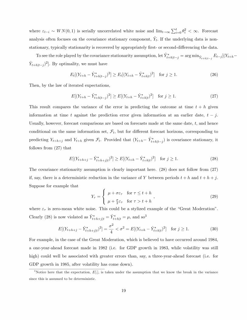
To see the role played by the covariance stationarity assumption, let Y ∗t+h|t−j = arg minYt+h|t−jEt−j [(Yt+h−

Yt+h|t−j)2]. By optimality, we must have

Et[(Yt+h − Y ∗t+h|t−j)2] ≥ Et[(Yt+h − Y ∗t+h|t)

2] for j ≥ 1. (26)

Then, by the law of iterated expectations,

E[(Yt+h − Y ∗t+h|t−j)2] ≥ E[(Yt+h − Y ∗t+h|t)

2] for j ≥ 1. (27)

This result compares the variance of the error in predicting the outcome at time t + h given

information at time t against the prediction error given information at an earlier date, t − j.

Usually, however, forecast comparisons are based on forecasts made at the same date, t, and hence

conditional on the same information set, Ft, but for different forecast horizons, corresponding to

predicting Yt+h+j and Yt+h given Ft. Provided that (Yt+h− Y ∗t+h|t−j) is covariance stationary, it

follows from (27) that

E[(Yt+h+j − Y ∗t+h+j|t)2] ≥ E[(Yt+h − Y ∗t+h|t)

2] for j ≥ 1. (28)

The covariance stationarity assumption is clearly important here. (28) does not follow from (27)

if, say, there is a deterministic reduction in the variance of Y between periods t+ h and t+ h+ j.

Suppose for example that

Yτ =

µ+ σετ for τ ≤ t+ h

µ+ σ2 ετ for τ > t+ h

, (29)

where ετ is zero-mean white noise. This could be a stylized example of the “Great Moderation”.

Clearly (28) is now violated as Y ∗t+h+j|t = Y ∗t+h|t = µ, and so3

E[(Yt+h+j − Y ∗t+h+j|t)2] =

σ2

4< σ2 = E[(Yt+h − Y ∗t+h|t)

2] for j ≥ 1. (30)

For example, in the case of the Great Moderation, which is believed to have occurred around 1984,

a one-year-ahead forecast made in 1982 (i.e. for GDP growth in 1983, while volatility was still

high) could well be associated with greater errors than, say, a three-year-ahead forecast (i.e. for

GDP growth in 1985, after volatility has come down).3Notice here that the expectation, E[.], is taken under the assumption that we know the break in the variance

since this is assumed to be deterministic.

19

4.1 Fixed event forecasts

Under covariance stationarity, studying the precision of a sequence of forecasts Yt|t−h is equivalent

to comparing the precision of Yt+h|t for different values of h. However, this equivalence need not

hold when the predicted variable, Yt, is not covariance stationary. One way to deal with non-

stationarities such as the break in the variance in (29) is to hold the forecast ‘event’fixed, while

varying the time to the event, h. In this case the forecast optimality test gets based on (27) rather

than (28). Forecasts where the target date, t, is kept fixed, while the forecast horizon varies are

commonly called fixed-event forecasts, see Clements (1997) and Nordhaus (1987).

To see how this works, notice that, by forecast optimality,

Et−hS [(Yt − Y ∗t|t−hL)2] ≥ Et−hS [(Yt − Y ∗t|t−hS )2] for hL ≥ hS . (31)

Moreover, by the law of iterated expectations,

E[(Yt − Y ∗t|t−hL)2] ≥ E[(Yt − Y ∗t|t−hS )2] for hL ≥ hS . (32)

This result is quite robust. For example, with a break in the variance, (29), we have Y ∗t|t−hL =

Y ∗t|t−hS = µ, and

E[(Yτ − Y ∗τ |τ−hL)2] = E[(Yτ − Y ∗τ |τ−hS )2] =

σ2 for τ ≤ t+ h

σ2/4 for τ > t+ h.

As a second example, suppose we let the mean of a time-series be subject to a probabilistic

break that only is known once it has happened. To this end, define an absorbing state process,

sτ ∈ Fτ , such that s0 = 0 and Pr(sτ = 0|sτ−1 = 0) = π for all τ . Consider the following process:

yτ = µ+ sτ∆µ + (σ + sτ∆σ)ετ , ετ ∼ (0, 1).

Suppose we condition on st−h = 0, st−h+1 = 1, so the permanent break happens at time t− h+ 1.

Then

Y ∗t|t−j =

µ+ π∆µ for j ≥ h

µ+ ∆µ for j ≤ h− 1,

and so we have the expected loss

Et−j [(Yt − Y ∗t|t−j)2] =

(1− π)2∆2µ + (σ + ∆σ)2 for j ≥ h

(σ + ∆σ)2 for j ≤ h− 1.

20

Once again, monotonicity continues to hold for the fixed-event forecasts, i.e. for hL > hS and for

all t:

E[(Yt − Y ∗t|t−hL)2] ≥ E[(Yt − Y ∗t|t−hS )2].

4.2 A general class of non-stationary processes

Provided that a fixed-event setup is used, we next show that the variance bound results pertain to

a more general class of stochastic processes that do not require covariance stationarity.

Assumption S2: The target variable, Yt, is generated by

Yt = f(t, θ) +∞∑i=0

θitεt−i. (33)

where f(t, θ) captures deterministic parts (e.g. seasonality or trends), Y0 represents the initial

condition, εt ∼ WN(0, σ2ε) is serially uncorrelated mean-zero white noise, and, for all t, θit is a

sequence of deterministic coeffi cients such that∑∞

i=0 θ2it <∞ for all t.

Assumption S1 (covariance stationarity) is suffi cient for S2, and further implies that the coeffi -

cients in the representation are not functions of t, i.e., θit = θi ∀t. However Assumption S2 allows

for deviations from covariance stationarity that can be modeled via deterministic changes in the

usual Wold decomposition weights, θi. For example, it may be that, due to a change in economic

policy or the economic regime, the impulse response function changes after a certain date. For the

example in (29), we get

θ0,τ =

σ for τ ≤ t+ h

σ2 for τ > t+ h

, (34)

while θi,τ = 0 for all i ≥ 1.

It is possible to show that the natural extensions of the inequality results established in Corol-

laries 1, 2, 3, 4 and 5 also hold for this class of processes:

21

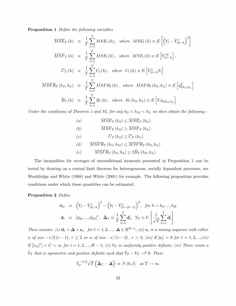
Proposition 1 Define the following variables

MSET (h) ≡ 1

T

T∑t=1

MSEt (h) , where MSEt (h) ≡ E[(Yt − Y ∗t|t−h

)2]

MSF T (h) ≡ 1

T

T∑t=1

MSFt (h) , where MSFt (h) ≡ E[Y ∗2t|t−h

],

CT (h) ≡ 1

T

T∑t=1

Ct (h) , where Ct (h) ≡ E[Y ∗t|t−hYt

]MSFRT (hS , hL) ≡ 1

T

T∑t=1

MSFRt (h) , where MSFRt (hS , hL) ≡ E[η2t|hS ,hL

]BT (h) ≡ 1

T

T∑t=1

Bt (h) , where Bt (hS , hL) ≡ E[Ytηt|hS ,hL

]Under the conditions of Theorem 1 and S2, for any hS < hM < hL we then obtain the following :

(a) MSET (hS) ≤MSET (hL)

(b) MSF T (hS) ≥MSF T (hL)

(c) CT (hS) ≥ CT (hL)

(d) MSFRT (hS , hM ) ≤MSFRT (hS , hL)

(e) MSFRT (hS , hL) ≤ 2BT (hS , hL)

The inequalities for averages of unconditional moments presented in Proposition 1 can be

tested by drawing on a central limit theorem for heterogeneous, serially dependent processes, see

Wooldridge and White (1988) and White (2001) for example. The following proposition provides

conditions under which these quantities can be estimated.

Proposition 2 Define

dht ≡(Yt − Y ∗t|t−h

)2−(Yt − Y ∗t|t−(h−1)

)2, for h = h2, ..., hH

dt ≡ [d2t, ..., dHt]′ , ∆T ≡

1

T

T∑t=1

d′t, VT ≡ V[

1√T

T∑t=1

d′t

]Then assume: (i) dt = ∆ + εt, for t = 1, 2, ..., ∆ ∈ RH−1; (ii) εt is a mixing sequence with either

φ of size −r/2 (r − 1), r ≥ 2 or α of size −r/ (r − 2) , r > 2; (iii) E [εt] = 0 for t = 1, 2, ...;(iv)

E [|εit|r] < C < ∞ for i = 1, 2, ...,H − 1; (v) VT is uniformly positive definite; (vi) There exists a

VT that is symmetric and positive definite such that VT − VT →p 0. Then:

V−1/2T

√T(∆T −∆

)⇒ N (0, I) as T →∞.

22

Thus we can estimate the average of unconditional moments with the usual sample average, with

the estimator of the covariance matrix suitably adjusted, and then conduct the test of inequalities

using Wolak’s (1989) approach.

4.3 Model misspecification

A natural question to ask is whether the forecast optimality tests presented so far are really tests of

forecast optimality or, rather, test that forecasters use consistent models in updating their forecasts

as the horizon changes. As we indicated earlier, the optimality tests that rely exclusively on the

forecasts−and thus exclude information on the outcome variable−test for consistency in forecasters’

revisions. This raises the question whether our tests are valid if forecasters use different and possibly

misspecified models at different horizons−a situation that might arise if forecasters use the ‘direct’

approach of fitting separate models to each forecast horizon as opposed to the ‘iterated’approach

where a single model is fitted to the shortest horizon and then iterated on to obtain multi-step

forecasts.

The variance bounds remain valid in situations where forecasters use misspecified models. They

require, however, that forecasters realize if they are using a suboptimal short-horizon model whose

predictions are dominated by the forecasts from a long-horizon model. Consider, for example,

the hypothetical situation where the (misspecified) one-step forecasting model delivers less precise

forecasts than, say, a two-step forecasting model. The variance bound results then require that

forecasters realize this and either switch to using the two-period forecasts outright (as in the

example below) or improve upon their one-step forecasting model.

To illustrate this, consider a simple MA(2) specification:4

Yt = εt + θεt−2, (35)

where εt ∼ (0, σ2ε) is white noise, and suppose that forecasters generate h−step forecasts by re-

gressing Yt on Yt−h. In particular, one-period forecasts are based on the model

Yt = β1yt−1 + ut.

It is easily verified for this process that p lim(β1) = 0, so Yt|t−1 = 0, and E[(Yt−Yt|t−1)2] = σ2ε(1+θ2).

4We are grateful to Ken West for proposing this example.

23

Turning next to the two-period forecast horizon, suppose the forecaster regresses Yt on Yt−2,

Yt = β2Yt−2 + ut,

where p lim(β2) = θ/(1 + θ2). This means that Yt|t−2 = θ(εt−2 + θεt−4)/(1 + θ2), so

E[(Yt − Yt|t−2)2] = E

[(εt +

θ(1 + θ2)− θ1 + θ2

εt−2 −θ2

1 + θ2εt−4

)2]

= σ2ε

(1 +

θ6 + θ4

(1 + θ2)2

)= σ2ε

(1 +

θ4

1 + θ2

).

It is easily seen that, in this case,

E[(Yt − Yt|t−2)2] ≤ E[(Yt − Yt|t−1)2],

seemingly in contradiction of the MSE inequality (2). The reason the MSE inequality fails in this

example is that optimizing forecasters should realize, at time t−1, that they are using a misspecified

model and that in fact the forecast from the previous period, Yt|t−2, produces a lower MSE. Hence,

in this example a better forecast at time t− 1 is Yt|t−1= Yt|t−2 = θ(εt−2 + θεt−4)/(1 + θ2).

Notice also that the mean squared forecast variance bound (6) is violated here since

var(Yt|t−1) = 0 < var(Yt|t−2) = σ2εθ2/(1 + θ2).

Thus, clearly the forecaster in this example is not producing optimal forecasts.

This example also illustrates that our variance bounds can be used to identify suboptimal

forecasts and hence help to improve on misspecified models.

In some special situations, by virtue of being weak inequalities, the variance inequality tests

may not have power to detect a sub-optimal forecast. This situation arises, for example, when all

forecasts are constant, i.e. Yt|t−h = c for all h. For this “broken clock” forecast, MSE-values are

constant across horizons, forecast variances are zero as are the forecast revisions and the covariance

between forecasts and actual values. This is a very special case, however, that rules out any

variation in the forecast and so can be deemed empirically irrelevant.

5 Monte Carlo Simulations

There is little existing evidence on the finite sample performance of forecast optimality tests, par-

ticularly when multiple forecast horizons are simultaneously involved. Moreover, we have proposed

24

a set of new optimality tests which take the form of bounds on second moments of the data and

require using the Wolak (1989) test of inequality constraints which also has not been widely used

so far.5 For these reasons it is important to shed light on the finite sample performance of the

various forecast optimality tests. Unfortunately, obtaining analytical results on the size and power

of these tests for realistic sample sizes and types of alternatives is not possible To overcome this,

we use Monte Carlo simulations of a variety of different scenarios.We next describe the simulation

design and then present the size and power results.

5.1 Simulation design

To capture persistence in the underlying data, we consider a simple AR(1) model for the data

generating process:

Yt = µy + φ(Yt−1 − µy

)+ εt, t = 1, 2, ..., T = 100 (36)

εt ∼ iid N(0, σ2ε

).

We calibrate the parameters to quarterly US CPI inflation data:

φ = 0.5, σ2y = 0.5, µy = 0.75.

Optimal forecasts for this process are given by:

Y ∗t|t−h = Et−h [Yt]

= µy + φh(Yt−h − µy

)We consider all horizons between h = 1 and H, and we set H ∈ { 4 , 8 }.

5.1.1 Measurement error

The performance of optimality tests that rely on the target variable versus tests that only use

forecasts is likely to be heavily influenced by measurement errors in the underlying target variable,

Yt. To study the effect of this, we assume that the target variable, Yt, is observed with error, ψt

Yt = Yt + ψt, ψt ∼ iid N(0, σ2ψ

).

5One exception is Patton and Timmermann (2009) who provide some evidence on the performance of the Wolak

test in the context of tests of financial return models.

25

We consider three values for the magnitude of the measurement error, σψ, calibrated relative to

the standard deviation of the underlying variable, σy, namely (i) zero, σψ = 0 (as for CPI); (ii)

medium, σψ/σy = 0.65 (as for GDP growth first release data);6 and (iii) high, σψ/σy = 1.

5.1.2 Sub-optimal forecasts

To study the power of the optimality tests, we consider a variety of ways in which the forecasts can

be suboptimal. First, we consider forecasts that are contaminated by the same level of noise at all

horizons:

Yt|t−h = Y ∗t|t−h + σξ,hZt,t−h, Zt,t−h ∼ iid N (0, 1) ,

where σξ,h = 0.65σy for all h and thus has the same magnitude as the medium level measurement

error.

Forecasts may alternatively be affected by noise whose standard deviation is increasing in the

horizon, ranging from zero for the short-horizon forecast to 2 × 0.65σy for the longest forecast

horizon (H = 8):

σξ,h =2 (h− 1)

7× 0.65σy, for h = 1, 2, ...,H ≤ 8.

Forecasts affected by noise whose magnitude is decreasing in the horizon (from zero for h = 8 to

2× 0.65σy for h = 1) take the form:

σξ,h =2 (8− h)

7× 0.65σy, for h = 1, 2, ...,H ≤ 8.

Finally, consistent with example 3 we consider forecasts with either “sticky”updating or, con-

versely, “overshooting”:

Yt|t−h = γY ∗t|t−h + (1− γ)Y ∗t|t−h−1, for h = 1, 2, ...,H.

To capture “sticky” forecasts we set γ = 1/2, whereas for “overshooting” forecasts we set

γ = 1.5.

Tests based on forecast revisions may have better finite-sample properties than tests based on

the forecasts themselves, particularly when the underlying process is highly persistent.

6The “medium” value is calibrated to match US GDP growth data, as reported by Faust, Rogers and Wright

(2005).

26

5.2 Results from the simulation study

Table 1 reports the size of the various tests for a nominal size of 10%. Results are based on 1,000

Monte Carlo simulations and a sample of 100 observations. The variance bounds tests are clearly

under-sized, particularly for H = 4, where none of the tests have a size above 4%. In contrast, the

MZ Bonferroni bound is over-sized.7 The vector MZ test is also hugely oversized, while the size

of the univariate optimal revision regression is close to the nominal value of 10%. Because of the

clear size distortions to the MZ Bonferroni bound and the vector MZ regression, we do not further

consider those tests in the simulation study.

Turning to the power of the various forecast optimality tests, Table 2 reports the results of our

simulations, using the three measurement noise scenarios (constant, increasing and decreasing noise)

and the sticky updating and overshooting schemes, respectively. In the first scenario with equal

noise across different horizons (Panel A), neither the MSE, MSF, MSFR or decreasing covariance

bounds have much power to detect deviations from forecast optimality. This holds across all three

levels of measurement error. In contrast, the covariance bound on forecast revisions has excellent

power to detect this type of deviation from optimality−close to 100%−particularly when the short-

horizon forecast, Yt|t−1, which is not affected by noise, is used as the dependent variable.8 The power

is somewhat weaker when the covariance bound test is adopted on the actual variable, although it

improves by roughly 10% when the measurement error is reduced from the high value to zero. The

univariate optimal revision regression (21) also has excellent power properties, particularly when

the dependent variable is the short-horizon forecast.

The scenario with additive measurement noise that increases in the horizon, h, is ideal for the

decreasing MSF test since now the variance of the long-horizon forecast is artificially inflated in

contradiction of (6). Thus, as expected, Panel B of Table 2 shows that this test has very good power

under this scenario: 42% in the case with four forecast horizons, rising to 100% in the case with

eight forecast horizons. The MSE and MSFR bounds have zero power for this type of deviation

from forecast optimality. The covariance bound based on the predicted variable has power around

7Conventionally, Bonferroni bounds tests are conservative and tend to be undersized. Here, the individual MZ

regression tests are even more oversized than shown here, so the Bonferroni bound leads to a reduction in the size of

the test which is still oversized.8The covariance bound (14) works so well because noise in the forecast increases E[η2t|hS ,hL ] without affecting

E[Ytηt|hS ,hL ], thereby making it less likely that E[Ytηt|hS ,hL − η2t|hS ,hL ] ≥ 0 holds.

27

15% when H = 4, which increases to a power of 90-95% when H = 8. The covariance bound with

the actual value replaced by the short-run forecast, (16), has the highest power among all tests,

with power of 70% when H = 4 and power of 100% when H = 8. This is substantially higher than

the power of the univariate optimal revision regression test (21) which has power close to 10-15%

when conducted on the actual values and power of 60% when the short-run forecast is used as the

dependent variable. 9

Panel C of Table 2 shows that the scenario with noise in the forecast that decreases as a function

of the forecast horizon, h, gives rise to high power for the increasing MSE test and also for the MSFR

test with power again being much higher when H = 8 compared to when H = 4. However, once

again the covariance bound test and the univariate optimal revision regression (21) have superior

power.

The univariate optimal revision regression (21) and the covariance bound test have stronger

power in the scenarios with noise that is either constant or decreasing in the forecast horizon, h,

because the precision of the forecasts is much better at short horizons. Hence, the greater the noise

that is added to the short horizon forecasts, the better these tests are able to detect ineffi ciency of

the forecast.

The next scenario assumes sticky updating in the forecasts. In this case, shown in Panel D

of Table 2, only the univariate optimal revision regression (21) seems to have much power to

detect deviations from a fully rational forecast. The power lies between 27% and 60% for this test

when the regression is based on the actual variable, and grows stronger as a result of reducing the

measurement error from the high value to zero. Interestingly, power is close to 100% when the

univariate optimal revision regression is based on the short-term forecasts.

In the final scenario with overshooting, shown in Panel E of Table 2, none of the tests has

particularly high power. However, the univariate optimal revision regression dominates with power

ranging between 23% and 58%, depending on the level of the measurement error and on how

many horizons are included. In this case power is actually stronger, the fewer constraints (H) are

considered.

We also consider using a Bonferroni bound to combine various tests based on actual values,

forecasts only or all tests. Results for these tests are shown at the bottom of tables 1 and 2.

9For this case, Yt|t−hH is very poor, but this forecast is also very noisy and so deviations from rationality can be

relatively diffi cult to detect.

28

In all cases we find that the size of the tests falls well below the nominal size, as expected for

a Bonferroni-based test, although the power seems to be quite high and comparable to the best

among the individual tests.

In conclusion, viewed across all four scenarios, the covariance bound test performs best among

all the second-moment bounds. Interestingly, it generally performs much better than the MSE

bound which is the most commonly known variance bound. Among the regression tests, excellent

performance is found for the univariate optimal revision regression, particularly when the test uses

the short-run forecast as the dependent variable. This test tends to have superior power properties

and performs well across most deviations from forecast effi ciency. Either the covariance test or

the univariate optimal revision regression have the highest power in all the experiments considered

here with the covariance bound test being best in the realistic case where the noise in the forecasts

increases with the horizon. Bonferroni bound tests conducted on the regression and second moment

tests are also found to have good properties, pooling the information across various individual tests.

6 Empirical Application

As an empirical illustration of the forecast optimality tests, we next evaluate the Federal Reserve

“Greenbook”forecasts of GDP growth, the GDP deflator and CPI inflation. Data are from Faust

and Wright (2009), who carefully extracted the Greenbook forecasts and actual values from real-

time Fed publications.10 We use quarterly observations of the target variable over the period from

1982Q1 to 2000Q4. Forecasts begin with the current quarter and run up to eight quarters ahead

in time. However, since the forecasts have many missing observations at the longest horizons and

we are interested in aligning the data in “event time”, we only study horizons up to five quarters,

i.e., h = 0, 1, 2, 3, 4, 5. A few quarterly observations are missing, leaving a total of 69 observations.

Empirical results are reported in Table 3. The key findings are as follows. For GDP growth

we observe a strong rejection of internal consistency via the univariate optimal revision regression

that uses the short-run forecast as the target variable, (24), and a mild violation of the increasing

mean-squared forecast revision test, (11).

Turning to the GDP deflator, we find that several tests reject forecast optimality. In particular,

the tests for a decreasing covariance, the covariance bound on forecast revisions, a decreasing

10We are grateful to Jonathan Wright for providing the data.

29

mean squared forecast, and the univariate optimal revision regression test all lead to rejections.

Figure 1 illustrates the rejection of the variance bound based on the forecasts and shows that, in

contradiction with (6) the MSF is not weakly decreasing in the horizon, h. In fact, the MSF is

higher for h = 5 than for h = 0.

Finally, for the CPI inflation rate we find a violation of the bound on the variance of the

revisions, (11), and a rejection through the univariate optimal revision regression.

For all three variables, the Bonferroni-based combination test rejects multi-horizon forecast

optimality at the 5% level. The type of rejections gives some clues as to possible sources of sub-

optimality.

The source of some of the rejections of forecast optimality is further illustrated in Figures 1-3.

For each of the series, Figure 1 plots the mean squared errors and variance of the forecasts on

top of each other. Under the null of forecast optimality, the forecast and forecast error should

be orthogonal and the sum of these two components should be constant across horizons. Clearly,

this does not hold here, particularly for the GDP deflator and CPI inflation series. As shown

in Figure 2−which plots the mean squared error and forecast variances separately−the variance

of the forecast in fact increases in the horizon for the GDP deflator, and it follows an inverse

U−shaped pattern for CPI inflation, both in apparent contradiction of the decreasing forecast

variance property established earlier.

Figure 3 plots mean squared errors and mean squared forecast revisions against the forecast

horizon. Whereas the mean squared forecast revisions are mostly increasing as a function of the

forecast horizon for the two inflation series, for GDP growth we observe the opposite pattern,

namely a very high mean squared forecast revision at the one-quarter horizon, followed by lower

values at longer horizons. This is the opposite of what we would expect and so explains the (weak)

rejection of forecast optimality for this case.

The Monte Carlo simulations are closely in line with our empirical findings. Rejections of

forecast optimality come mostly from the covariance bound (14), (16) and the univariate optimal

revision regressions (21), (24). Moreover, for GDP growth, rejections tend to be stronger when

only the forecasts are used. This makes sense since this variable is likely to be most affected by

data revisions and measurement errors.

30

7 Conclusion

In this paper we propose several new tests of forecast optimality that exploit information from

multi-horizon forecasts. Our new tests are based on (weak) monotonicity properties of second

moment bounds that must hold across forecast horizons and so are joint tests of optimality across

several horizons. We show that monotonicity tests, whether conducted on the squared forecast

errors, squared forecasts, squared forecast revisions or the covariance between the target variable

and the forecast revision can be restated as inequality constraints on regression models and that

econometric methods proposed by Gourieroux et al. (1982) and Wolak (1987, 1989) can be adopted.

Suitably modified versions of these tests conducted on the sequence of forecasts or forecast revisions

recorded at different horizons can be used to test the internal consistency properties of an optimal

forecast, thereby side-stepping the issues that arise for conventional tests when the target variable

is either missing or observed with measurement error.

Simulations suggest that the new tests are more powerful than extant ones and also have better

finite sample size. In particular a new covariance bound test that constrains the variance of forecast

revisions by their covariance with the outcome variable and a univariate joint regression test that

includes the long-horizon forecast and all interim forecast revisions generally have good power to

detect deviations from forecast optimality. These results show the importance of testing the joint

implications of forecast rationality across multiple horizons when data is available. An empirical

analysis of the Fed’s Greenbook forecasts of inflation and output growth corroborates the ability

of the new tests to detect evidence of deviations from forecast optimality.

Our analysis in this paper assumed squared error loss. However, many of the results can be

extended to allow for more general loss functions with known shape parameters. For example,

the MSE bound is readily generalized to a bound based on non-decreasing expected loss as the

horizon grows, see Patton and Timmermann (2007a). Similarly, the orthogonality regressions can

be extended to use the generalized forecast error, which is essentially the score associated with the

forecaster’s first order condition, see Patton and Timmermann (2010). Allowing for the case with

a parametric loss function but unknown (estimated) parameters is more involved and is a topic we

leave for future research.

31

have Y ∗t|t−h1 = Et−h1 [Yt] . Consider a first-stage regression of Yt on Y ∗t|t−h1 (without a constant).

Following the steps in the proof of Corollary 7, this yields a coeffi cient of one, and regression

residuals are e∗t|t−hS ≡ Yt − Y ∗t|t−hS . Next consider a regression of Y∗t|t−hj on Y

∗t|t−h1 (again without

a constant) for each j = 2, 3, ...,H, and let the slope coeffi cients from these regressions be denoted

γj . Finally consider a regression of the residuals from the first regression on the matrix of residuals

from the latter H − 1 regressions, namely:

e∗t|t−h1 = δ0 + δ2

(Y ∗t|t−h2 − γ2Y

∗t|t−h1

)+ ...+ δH

(Y ∗t|t−hH − γH Y

∗t|t−h1

)+ ξt.

Since forecast optimality implies Et−h1[e∗t|t−h1

]= 0, we then have δ0 = δ2 = ... = δH = 0. By

the Frisch-Waugh-Lovell theorem we know that δ0 = α, δ2 = λ2, ..., δH = λH . Thus the population

values of (α, λ2, .., λH) are zero, and the population value of λ1 is thus one. This implies that

α = 0, β1 = 1, β2 = 1,...,βH = 1, as claimed.

Proof of Corollary 9. (a) Under optimality, βh = Cov[Y ∗t|t−h1 , Y

∗t|t−hj

]/V[Y ∗t|t−hj

]=

Cov[Y ∗t|t−hj + ηt|h1,hj , Y

∗t|t−hj

]/V[Y ∗t|t−hj

]= V

[Y ∗t|t−hj

]/V[Y ∗t|t−hj

]= 1, and α = E

[Y ∗t|t−h1

]−

βE[Y ∗t|t−hj

]= E [Yt]− E [Yt] = 0.

(b) Follows using the same steps as the proof of part (b) of Corollary 8, noting that Y ∗t|t−h2 =

Et−h2 [Yt] = Et−h2

[Y ∗t|t−h1

]by the LIE, and that Et−h2

[Y ∗t|t−h1 − Y

∗t|t−h2

]≡ Et−h2

[ηt|h1,h2

]= 0.

Proof of Proposition 1. Throughout the proof we will use the fact that

Y ∗t|t−h = Et−h [Yt] = Et−h

[f (t, θ) +

∞∑i=0

θitεt−i

]= f (t, θ) +

∞∑i=h

θitεt−i

and e∗t|t−h ≡ Yt − Y ∗t|t−h =h−1∑i=0

θitεt−i

(a) From above we have

E[e∗2t|t−h

]= V

[e∗t|t−h

]= V

[h−1∑i=0

θitεt−i

]= σ2ε

h−1∑i=0

θ2it

thus E[e∗2t|t−hL

]− E

[e∗2t|t−hS

]= σ2ε

hL−1∑i=0

θ2it − σ2εhS−1∑i=0

θ2it = σ2ε

hL−1∑i=hS

θ2it ≥ 0

which implies that MSEt (hS) ≤MSEt (hL) for all t. This further implies that

MSET (hS) ≡ 1

T

T∑t=1

MSEt (hS) ≤ 1

T

T∑t=1

MSEt (hL) ≡MSET (hL) for all T .

34

The proofs of (b)-(e) all follow similar extensions as used in part (a) and are omitted in the interests

of brevity.

Proof of Proposition 2. Follows from Exercise 5.21 of White (2001).

References

[1] Capistran, Carlos, 2007, Optimality Tests for Multi-Horizon Forecasts. Manuscript no 2007-14,Banco de Mexico.

[2] Clements, Michael P., 1997, Evaluating the Rationality of Fixed-Event Forecasts. Journal ofForecasting 16, 225-239.

[3] Clements, Michael P., 2009, Internal consistency of survey respondents’ forecasts: Evidencebased on the Survey of Professional Forecasters. In The Methodology and Practice of Econo-metrics. A Festschrift in Honour of David F. Hendry. eds. Jennifer L. Castle and Neil Shephard.Oxford University Press. Chapter 8, 206 - 226.

[4] Clements, Michael P., and David F. Hendry, 1998, Forecasting Economic Time Series. Cam-bridge. Cambridge University Press.

[5] Corradi, Valentina, Andres Fernandez, and Norman R. Swanson, 2009, Information in theRevision Process of Real-Time Datasets, Journal of Business Economics and Statistics 27,455-467.

[6] Croushore, Dean, 2006, Forecasting with Real-Time Macroeconomic Data. Pages 961-982 inG. Elliott, C. Granger and A. Timmermann (eds.) Handbook of Economic Forecasting, NorthHolland: Amsterdam.

[7] Croushore, Dean and Tom Stark, 2001, A Real-Time Data Set for Macroeconomists. Journalof Econometrics 105, 111-130.

[8] Davies, A. and K. Lahiri, 1995, A New Framework for Analyzing Survey Forecasts usingThree-Dimensional Panel Data, Journal of Econometrics, 68, 205-227.

[9] Diebold, Francis X., 2001, Elements of Forecasting. 2nd edition. Ohio: South-Western.

[10] Diebold, Francis X. and Glenn D. Rudebusch, 1991, Forecasting Output with the CompositeLeading Index: A Real-Time Analysis, Journal of the American Statistical Association, 86,603-610.

[11] Faust, Jon, John Rogers and Jonathan Wright, 2005, News and Noise in G-7 GDP Announce-ments. Journal of Money, Credit and Banking 37, 403-419.

[12] Faust, Jon and Jonathan Wright, 2009, Comparing Greenbook and Reduced Form Forecastsusing a Large Realtime Dataset. Journal of Business and Economic Statistics 27, 468-479.

35

[13] Giacomini, Raffaella and Halbert White, 2006, Tests of Conditional Predictive Ability. Econo-metrica 74, 6, 1545-1578.

[14] Gourieroux, C., A. Holly and A. Monfort, 1982, Likelihood Ratio Test, Wald Test, and Kuhn-Tucker Test in Linear Models with Inequality Constraints on the Regression Parameters.Econometrica 50, 63-80.

[15] Marcellino, Massimiliano, James H. Stock and Mark W. Watson, 2006, A comparison of directand iterated multistep AR methods for forecasting macroeconomic time series.’ Journal ofEconometrics 135, 499—526.

[16] Mincer, Jacob, and Victor Zarnowitz, 1969, The Evaluation of Economic Forecasts, in J.Mincer (ed.) Economic Forecasts and Expectations, National Bureau of Economic Research,New York.

[17] Moon, Roger, Frank Schorfheide, Eleonora Granziera and Mihye Lee, 2009, Inference for VARsidentified with sign restrictions. Mimeo, University of Southern California and University ofPennsylvania.

[18] Newey, Whitney K., and Kenneth D. West, 1987, A Simple, Positive Semidefinite, Het-eroskedasticity and Autocorrelation Consistent Covariance Matrix, Econometrica, 55, 703-708.

[19] Nordhaus, William D., 1987, Forecasting Effi ciency: Concepts and Applications. Review ofEconomics and Statistics 69, 667-674.

[20] Patton, Andrew J., and Allan Timmermann, 2007a, Properties of optimal forecasts underasymmetric loss and nonlinearity. Journal of Econometrics, 140(2), 884-918.

[21] Patton, Andrew J., and Allan Timmermann, 2007b, Testing Forecast Optimality under Un-known Loss. Journal of the American Statistical Association 102, 1172-1184.

[22] Patton, Andrew J., and Allan Timmermann, 2008, Predictability of output growth and infla-tion: A multi-horizon survey approach. Unpublished manuscript, Duke and UCSD.

[23] Patton, Andrew J., and Allan Timmermann, 2009, Monotonicity in Asset Returns; New Testswith Applications to the Term Structure, the CAPM, and Portfolio Sorts. Forthcoming inJournal of Financial Economics.

[24] Patton, Andrew J. and Allan Timmermann, 2010, Generalized Forecast Errors, A Change ofMeasure and Forecast Optimality. Forthcoming in T. Bollerslev, J. Russell, and M. Watson,(eds.), Volatility and Time Series Econometrics: Essays in Honour of Robert F. Engle, OxfordUniversity Press.

[25] Schmidt, Peter, 1974, The Asymptotic Distribution of Forecasts in the Dynamic Simulationof an Econometric Model. Econometrica 42, 303-309.

[26] Timmermann, Allan, 1993, How Learning in Financial Markets Generates Excess Volatilityand Predictability in Stock Prices. Quarterly Journal of Economics 108(4), 1135-1145.

[27] West, Kenneth D., 1996, Asymptotic Inference about Predictive Ability. Econometrica 64,1067-84.

36

[28] West, Kenneth D., and Michael W. McCracken, 1998, Regression Based Tests of PredictiveAbility. International Economic Review 39, 817-840.

[29] White, Halbert, 2001, Asymptotic Theory for Econometricians, Second Edition, AcademicPress, San Diego.

[30] Wolak, Frank A., 1987, An Exact Test for Multiple Inequality and Equality Constraints in theLinear Regression Model. Journal of the American Statistical Association 82, 782-793.

[31] Wolak, Frank A., 1989, Testing Inequality Constraints in Linear Econometric Models. Journalof Econometrics 31, 205-235.

[32] Wooldridge, Jeffrey M., and Halbert White, 1988, Some Invariance Principles and CentralLimit Theorems for Dependent Heterogeneous Processes, Econometric Theory, 4, 210-230.

37

Table 1: Monte Carlo simulation of size of the inequality testsand regression-based tests of forecast optimality

H = 4 H = 8

Meas. error variance: High Med Zero High Med Zero

Inc MSE 1.9 1.7 1.1 7.8 6.4 8.3Dec COV 1.1 1.1 0.8 8.4 7.3 7.2COV bound 2.2 1.2 0.4 2.3 1.4 0.8Dec MSF 2.1 2.1 2.1 5.3 5.3 5.3Inc MSFR 0.4 0.4 0.4 5.5 5.5 5.5Dec COV, h=1 0.9 0.9 0.9 6.4 6.4 6.4COV bound, h=1 3.6 3.6 3.6 4.6 4.6 4.6Inc MSE & Dec MSF 1.5 1.3 0.8 8.3 8.2 9.1Inc MSE & Inc MSFR 1.1 0.8 0.6 7.2 6.7 6.5Univar MZ, Bonferroni 13.8 15.0 17.8 19.5 19.4 20.3Univar MZ, Bonferroni, h=1 16.0 16.0 16.0 19.2 19.2 19.2Vector MZ 39.8 38.0 31.2 63.0 62.0 58.8Vector MZ, h=1 25.2 25.2 25.2 52.4 52.4 52.4Univar opt. revision regr. 11.3 11.5 11.0 12.4 11.8 11.0Univar opt. revision regr., h=1 12.0 12.0 12.0 11.3 11.3 11.3Bonf, using actuals 3.9 4.2 3.6 7.4 7.6 8.0Bonf, using forecasts only 3.0 3.0 3.0 6.6 6.6 6.6Bonf, all tests 3.6 3.5 2.2 7.6 7.5 6.2

Notes: This table presents the outcome of 1,000 Monte Carlo simulations of the size of variousforecast optimality tests. Data is generated by a first-order autoregressive process with parameterscalibrated to quarterly US CPI inflation data, i.e. φ = 0.5, σ2y = 0.5 and µy = 0.75. We considerthree levels of error in the measured value of the target variable (high, median and zero). Optimalforecasts are generated under the assumption that this process (and its parameter values) are knownto forecasters. The simulations assume a sample of 100 observations and a nominal size of 10%.The inequality tests are based on the Wolak (1989) test and use simulated critical values based ona mixture of chi-squared variables. Rows with ‘h = 1’refer to cases where the one-period forecastis used in place of the predicted variable.

38

Table 2: Monte Carlo simulation of power of the inequality testsand regression-based tests of forecast optimality

H = 4 H = 8


PANEL A: Equal noise across all forecast horizonsInc MSE 7.5 6.8 6.8 13.4 12.4 12.6Dec COV 7.3 6.4 6.1 13.0 13.5 12.2COV bound 73.7 79.6 83.2 74.8 78.7 83.3Dec MSF 5.8 5.8 5.8 15.0 15.0 15.0Inc MSFR 9.9 9.9 9.9 14.8 14.8 14.8Dec COV, h=1 8.9 8.9 8.9 15.4 15.4 15.4COV bound, h=1 98.0 98.0 98.0 99.1 99.1 99.1Inc MSE & Dec MSF 7.8 7.6 6.9 27.3 26.7 26.0Inc MSE & Inc MSFR 8.2 7.3 7.0 23.4 23.3 23.0Univar opt. revision regr. 91.9 98.1 99.6 85.3 95.9 99.0Univar opt. revision regr., h=1 100.0 100.0 100.0 100.0 100.0 100.0Bonf, using actuals 83.4 94.0 98.5 78.7 89.8 96.7Bonf, using forecasts only 100.0 100.0 100.0 99.9 99.9 99.9Bonf, all tests 100.0 100.0 100.0 100.0 100.0 100.0

Notes: This table presents the outcome of 1,000 Monte Carlo simulations of the size of variousforecast optimality tests. Data is generated by a first-order autoregressive process with parameterscalibrated to quarterly US CPI inflation data, i.e. φ = 0.5, σ2y = 0.5 and µy = 0.75. We considerthree levels of error in the measured value of the target variable (high, median and zero). Optimalforecasts are generated under the assumption that this process (and its parameter values) are knownto forecasters. Power is then studied against sub-optimal forecasts obtained as follows: A: forecastsare contaminated by the same level of noise across all horizons; B: forecasts are contaminated bynoise that increases in the horizon; C: forecasts are contaminated by noise that decreases in thehorizon; D: Forecasts are updated in a sticky manner; E: forecasts overshoot their optimal values.The simulations assume a sample of 100 observations and a nominal size of 10%. Rows with ‘h = 1’refer to cases where the one-period forecast is used in place of the predicted variable.

39


H = 4 H = 8


PANEL B: Noise increases with the horizonInc MSE 0.2 0.2 0.0 0.0 0.0 0.0Dec COV 3.3 3.0 2.8 13.5 12.8 12.2COV bound 12.9 14.5 14.9 90.7 93.3 95.2Dec MSF 42.3 42.3 42.3 100.0 100.0 100.0Inc MSFR 0.0 0.0 0.0 0.0 0.0 0.0Dec COV, h=1 4.9 4.9 4.9 12.9 12.9 12.9COV bound, h=1 69.2 69.2 69.2 100.0 100.0 100.0Inc MSE & Dec MSF 25.5 25.3 23.2 99.8 99.8 99.8Inc MSE & Inc MSFR 0.2 0.0 0.0 0.0 0.0 0.0Univar opt. revision regr. 11.7 12.3 11.9 13.1 13.6 12.9Univar opt. revision regr., h=1 63.6 63.6 63.6 54.6 54.6 54.6Bonf, using actuals 7.9 9.2 9.2 80.1 84.1 86.6Bonf, using forecasts only 63.0 63.0 63.0 100.0 100.0 100.0Bonf, all tests 54.7 54.7 54.4 100.0 100.0 100.0

PANEL C: Noise decreases with the horizonInc MSE 71.3 79.8 87.1 100.0 100.0 100.0Dec COV 6.7 5.8 6.1 13.6 12.5 13.1COV bound 99.5 99.8 99.9 99.5 99.8 99.9Dec MSF 0.4 0.4 0.4 0.1 0.1 0.1Inc MSFR 55.9 55.9 55.9 100.0 100.0 100.0Dec COV, h=1 10.6 10.6 10.6 17.6 17.6 17.6COV bound, h=1 99.8 99.8 99.8 99.2 99.2 99.2Inc MSE & Dec MSF 50.8 59.6 69.1 100.0 100.0 100.0Inc MSE & Inc MSFR 79.6 83.1 88.8 100.0 100.0 100.0Univar opt. revision regr. 100.0 100.0 100.0 100.0 100.0 100.0Univar opt. revision regr., h=1 100.0 100.0 100.0 100.0 100.0 100.0Bonf, using actuals 100.0 100.0 100.0 100.0 100.0 100.0Bonf, using forecasts only 100.0 100.0 100.0 100.0 100.0 100.0Bonf, all tests 100.0 100.0 100.0 100.0 100.0 100.0

Notes: See notes to Panel A of this table on previous page.

40


H = 4 H = 8


PANEL D: Sticky updatingInc MSE 2.0 1.4 1.1 6.8 6.0 7.6Dec COV 2.1 2.1 2.1 9.2 8.7 8.5COV bound 0.9 0.7 0.4 1.2 0.8 0.5Dec MSF 4.8 4.8 4.8 8.2 8.2 8.2Inc MSFR 0.0 0.0 0.0 4.8 4.8 4.8Dec COV, h=1 2.4 2.4 2.4 7.4 7.4 7.4COV bound, h=1 2.7 2.7 2.7 4.3 4.3 4.3Inc MSE & Dec MSF 2.6 2.4 2.1 11.0 11.0 10.7Inc MSE & Inc MSFR 0.8 0.9 0.9 7.9 7.0 8.3Univar opt. revision regr. 33.2 44.8 59.1 27.5 35.2 49.9Univar opt. revision regr., h=1 99.5 99.5 99.5 98.9 98.9 98.9Bonf, using actuals 15.2 22.0 37.4 14.9 19.1 28.9Bonf, using forecasts only 97.5 97.5 97.5 93.3 93.3 93.3Bonf, all tests 96.3 96.2 96.2 89.4 89.4 89.4

PANEL E: Over-shootingInc MSE 2.9 2.4 2.2 8.8 8.0 7.3Dec COV 1.1 0.5 0.7 5.6 5.7 5.6COV bound 5.4 4.6 4.8 4.9 4.7 4.9Dec MSF 1.0 1.0 1.0 3.6 3.6 3.6Inc MSFR 2.5 2.5 2.5 8.1 8.1 8.1Dec COV, h=1 1.0 1.0 1.0 6.6 6.6 6.6COV bound, h=1 7.7 7.7 7.7 8.5 8.5 8.5Inc MSE & Dec MSF 1.2 0.9 0.7 6.6 7.3 6.5Inc MSE & Inc MSFR 2.0 2.1 1.9 10.1 9.5 7.1Univar opt. revision regr. 29.8 41.8 57.9 23.8 32.4 48.0Univar opt. revision regr., h=1 32.3 32.3 32.3 27.9 27.9 27.9Bonf, using actuals 13.5 23.3 38.0 8.7 14.8 28.2Bonf, using forecasts only 0.0 0.0 0.0 13.7 13.7 13.7Bonf, all tests 10.3 17.1 31.3 11.9 14.5 22.1

Notes: See notes to Panel A of this table on previous page.

41

Table 3: Forecast optimality tests for Greenbook forecasts

Series: Growth Deflator Inflation

Inc MSE 0.599 0.964 0.644Dec COV 0.898 0.058∗ 0.991COV bound 0.498 0.000∗ 0.009∗

Dec MSF 0.898 0.026∗ 0.725Inc MSFR 0.084∗ 0.936 0.624Dec COV, h=1 0.802 0.075∗ 0.795COV bound, h=1 0.216 0.010∗ 0.656Inc MSE & Dec MSF 0.934 0.126 0.616Inc MSE & Inc MSFR 0.250 0.992 0.749Univar opt. revision regr. 0.709 0.000∗ 0.001∗

Univar opt. revision regr., h=1 0.000∗ 0.009∗ 0.022∗

Bonf, using actuals 1.000 0.000∗ 0.004∗

Bonf, using forecasts only 0.000∗ 0.047∗ 0.108Bonf, all tests 0.000∗ 0.001∗ 0.012∗

Note: This table presents p-values from inequality- and regression tests of forecast optimalityapplied to quarterly Greenbook forecasts of GDP growth, the GDP deflator and CPI Inflation. Thesample covers the period 1982Q1-2000Q4. Six forecast horizons are considered, i.e., h = 0, 1, 2,3, 4, 5 and the forecasts are aligned in event time. The inequality tests are based on the Wolak(1989) test and use simulated critical values based on a mixture of chi-squared variables. Rowswith ‘h = 1’refer to cases where the one-period forecast is used in place of the predicted variable.

42

5 4 3 2 1 00

0.2

0.4

0.6

0.8

1

1.2

1.4Forecasts and f orecast errors

Forecast horizon

Varia

nce

MSEV[f orecast]V[actual]

Figure 1: Theoretical mean squared errors and forecast variances for an AR(1) process with uncon-ditonal variance of 1 and autoregressive coeffi cient of 0.8.

43

5 4 3 2 1 00

1

2

3

4GDP deflator

Forecast horizon

Var

ianc

e

5 4 3 2 1 00

1

2

3

4

5CPI inflation

Forecast horizon

Var

ianc

e

5 4 3 2 1 00

2

4

6

8GDP grow th

Forecast horizon

Var

ianc

e

MSEV[forecast]V[actual]

Figure 2: Mean squared errors and forecast variances, for US GDP deflator, CPI inflation andGDP growth.

44

5 4 3 2 1 00

1

2

3

4

5

6

7

forecast horizon

Meansquared forecast errors

5 4 3 2 1 00

1

2

3

4

5

6

7

forecast horizon

Meansquared forecast revisions

GDP growthCPI inflationGDP deflator

Figure 3: Mean squared errors (left panel) and mean-squared forecast revisions (right panel), forUS GDP deflator, CPI inflation and GDP growth.

45

New Tests of Forecast Optimality Across Multiple Horizons

Documents

Transcript of New Tests of Forecast Optimality Across Multiple Horizons