New Results on Quantum PropertyTesting

Sourav Chakraborty1, Eldar Fischer2, Arie Matsliah1, Ronaldde Wolf1

1 Centrum Wiskunde & Informatica, Amsterdam. RdW is partially supported by a Vidi grantfrom the Netherlands Organization for Scientific Research (NWO), and by the European

Commission under the Integrated Project Qubit Applications (QAP) funded by the ISTdirectorate as Contract Number 015848. sourav,ariem,rdewolf@cwi.nl

2 Computer Science Faculty, Israel Institute of Technology (Technion). Partially supportedby an ERC-2007-StG grant number 202405-2 and by an ISF grant number 1101/06.

eldar@cs.technion.ac.il

ABSTRACT. We present several new examples of speed-ups obtainable by quantum algorithms in thecontext of property testing.First, motivated by sampling algorithms, we consider probability distributions given in the form of anoracle f : [n] → [m]. Here the probability P f (j) of an outcome j ∈ [m] is the fraction of its domainthat f maps to j. We give quantum algorithms for testing whether two such distributions are identicalor ε-far in L1-norm. Recently, Bravyi, Hassidim, and Harrow [11] showed that if P f and Pg are bothunknown (i.e., given by oracles f and g), then this testing can be done in roughly

√m quantum queries

to the functions. We consider the case where the second distribution is known, and show that testingcan be done with roughly m1/3 quantum queries, which we prove to be essentially optimal. In contrast,it is known that classical testing algorithms need about m2/3 queries in the unknown-unknown caseand about

√m queries in the known-unknown case. Based on this result, we also reduce the query

complexity of graph isomorphism testers with quantum oracle access.While those examples provide polynomial quantum speed-ups, our third example gives a much largerimprovement (constant quantum queries vs polynomial classical queries) for the problem of testingperiodicity, based on Shor’s algorithm and a modification of a classical lower bound by Lachish andNewman [30]. This provides an alternative to a recent constant-vs-polynomial speed-up due to Aaron-son [1].

1 Introduction

Since the early 1990s, a number of quantum algorithms have been discovered that have muchbetter query complexity than their best classical counterparts [17, 34, 24, 4, 18, 5]. Aroundthe same time, the area of property testing gained prominence [9, 22, 19, 32]. Here the aim isto design algorithms that can efficiently test whether a given very large piece of data satisfiessome specific property, or is “far” from having that property.

Buhrman et al. [13] combined these two strands, exhibiting various testing problemswhere quantum testers are much more efficient than classical testers. There has been somerecent subsequent work on quantum property testing, such as the work of Friedl et al. [21]on testing hidden group properties, Atici and Servedio [6] on testing juntas, Inui and LeGall [28] on testing group solvability, Childs and Liu [15] on testing bipartiteness and expan-sion, Aaronson [1] on “Fourier checking”, and Bravyi, Hassidim, and Harrow [11] on testingdistributions. We will say more about the latter papers below.

In this paper we continue this line of research, coming up with a number of new exampleswhere quantum testers substantially improve upon their classical counterparts. It should benoted that we do not invent new quantum algorithms here—rather, we use known quantumalgorithms as subroutines in otherwise classical testing algorithms.

1.1 Distribution Testing

How many samples are needed to determine whether two distributions are identical or haveL1-distance more than ε? This is a fundamental problem in statistical hypothesis testing andalso arises in other subjects like property testing and machine learning.

We use the notation [n] = 1, 2, 3, . . . , n. For a function f : [n] → [m], we denote byP f the distribution over [m] in which the weight P f (j) of every j ∈ [m] is proportional tothe number of elements i ∈ [n] that are mapped to j. We use this form of representation fordistributions in order to allow queries. Namely, we assume that the function f : [n] → [m]is accessible by an oracle of the form |x〉|b〉 7→ |x〉|b⊕ f (x)〉, where x is a log n-bit string,b and f (x) are log m-bit strings and ⊕ is bitwise addition modulo two. Note that a classicalrandom sample according to a distribution P f can be simply obtained by picking i ∈ [n]uniformly at random and evaluating f (i). In fact, a classical algorithm cannot make a betteruse of the oracle, since the actual labels of the domain [n] are irrelevant. See Section F in theAppendix for more on the relation between sampling a distribution and querying a function.

We say that the distribution P f is known (or explicit) if the function f is given explicitly,and hence all probabilities P f (j) can be computed. P f is unknown (or black-box) if weonly have oracle access to the function f , and no additional information about f is given.Two distributions P f ,Pg defined by functions f , g : [n] → [m] are ε-far if the L1-distancebetween them is at least ε, i.e., ‖P f −Pg‖1 = ∑m

j=1 |P f (j)−Pg(j)| ≥ ε. Note that f = gimplies P f = Pg but not vice versa (for instance, permuting f leaves P f invariant). Twoproblems of testing distributions can be formally stated as follows:• unknown-unknown case. Given n, m, ε and oracle access to f , g : [n] → [m], how

many queries to f and g are required in order to determine whether the distributions P fand Pg are identical or ε-far?

1

• known-unknown case. Given n, m, ε, oracle access to f : [n] → [m] and a knowndistribution Pg (defined by an explicitly given function g : [n] → [m]), how manyqueries to f are required to determine whether P f and Pg are identical or ε-far?

If only classical queries are allowed (where querying the distribution means asking for arandom sample), the answers to these problems are well known. For the unknown-unknowncase Batu, Fortnow, Rubinfeld, Smith, and White [8] proved an upper bound of O(m2/3)on the query complexity, and Valiant [35] proved a matching (up to polylogarithmic factors)lower bound. For the known-unknown case, Goldreich and Ron [23] showed a lower bound ofΩ(√

m) queries and Batu, Fischer, Fortnow, Rubinfeld, Smith, and White [7] proved a nearlytight upper bound of O(

√m) queries.∗

Testing with Quantum Queries

Allowing quantum queries for accessing distributions, Bravyi, Hassidim, and Harrow [11]recently showed that the L1-distance between two unknown distributions can actually be es-timated up to small error with only O(

√m) queries. Their result implies an O(

√m) upper

bound on the quantum query complexity for the unknown-unknown testing problem definedabove. In this paper we consider the known-unknown case, and prove nearly tight bounds onits quantum query complexity.

THEOREM 1. Given n, m, ε, oracle access to f : [n] → [m] and a known distributionPg (defined by an explicitly given function g : [n] → [m]), the quantum query complexity

of determining whether P f and Pg are identical or ε-far is O(m1/3 log2 m log log mε5 ) = m1/3 ·

poly( 1ε , log m).

We prove Theorem 1 in two parts. First, in Section 3.1, we prove that with O(m1/3

ε2 )quantum queries it is possible to test whether a black-box distribution P f (defined by somef : [n] → [m]) is ε-close to uniform. We actually prove that this can be even done tolerantlyin a sense, meaning that a distribution that is close to uniform in the L∞ norm is acceptedwith high probability (see Theorem 10 for the formal statement). Then, in Section 3.2, we usethe bucketing technique (see Section 2.1) to reduce the task of testing closeness to a knowndistribution to testing uniformity.

We stress that the main difference between the classical algorithm of [7] and ours is thatin [7] they check the “uniformity” of the unknown distribution in every bucket by approximat-ing the corresponding L2 norms of the conditional distributions. It is not clear if one can gainanything (in the quantum case) using the same strategy, since we are not aware of any quan-tum procedure that can approximate the L2 norm of a distribution with less than

√m queries.

Hence, we reduce the main problem directly to the problem of testing uniformity. For thisreduction to work, the uniformity tester has to be tolerant in the sense mentioned above (seeSection 3.2 for details).

A different quantum uniformity tester was recently discovered (independently) in [11].We note that our version has the advantages of being tolerant, which is crucial for the appli-

∗These classical lower bounds are stated in terms of number of samples rather than number of queries, but it isnot hard to see that they hold in both models. In fact, the

√m classical query lower bound for the known-unknown

case follows by the same argument as the quantum lower bound in Appendix D.

2

cation above, and it has only polynomial dependence on ε (instead of exponential), which isessentially optimal.

Quantum Lower Bounds

Known quantum query lower bounds for the collision problem [2, 3, 29] imply that in bothknown-unknown and unknown-unknown cases roughly m1/3 quantum queries are required.In fact, the lower bound applies even for testing uniformity (see proof in Appendix D):

THEOREM 2. Given n, m, ε and oracle access to f : [n] → [m], the quantum query com-plexity of determining whether P f is uniform or ε-far from uniform is Ω(m1/3).

The main remaining open problem is to tighten the bounds on the quantum query com-plexity for the unknown-unknown case. It would be very interesting if this case could also betested using roughly m1/3 quantum queries. In Appendix E we show that the easiest way todo this (just reconstructing both unknown distributions up to small error) will not work—itrequires Ω(m/ log m) quantum queries.

1.2 Graph Isomorphism Testing

Fischer and Matsliah [20] studied the problem of testing graph isomorphism in the dense-graph model, where the graphs are represented by their adjacency matrices, and querying thegraph corresponds to reading a single entry from its adjacency matrix. The goal in isomor-phism testing is to determine, with high probability, whether two graphs G and H are isomor-phic or ε-far from being isomorphic, making as few queries as possible. (The graphs are ε-farfrom being isomorphic if at least an ε-fraction of the entries in their adjacency matrices needto be modified in order to make them isomorphic.)

In [20] two models were considered:• unknown-unknown case. Both G and H are unknown, and they can only be accessed

by querying their adjacency matrices.• known-unknown case. The graph H is known (given in advance to the tester), and the

graph G is unknown (can only be accessed by querying its adjacency matrix).As usual, in both models the query complexity is the worst-case number of queries

needed to test whether the graphs are isomorphic. [20] give nearly tight bounds of Θ(√|V|)

on the (classical) query complexity in the known-unknown model. For the unknown-unknownmodel they prove an upper bound of O(|V|5/4) and a lower bound of Ω(|V|) on the querycomplexity.

Allowing quantum queries†, we can use our aforementioned results to prove the follow-ing query-complexity bounds for testing graph isomorphism (see proof in Appendix C):

THEOREM 3. The quantum query complexity of testing graph isomorphism in the known-unknown case is Θ(|V|1/3), and in the unknown-unknown case it is between Ω(|V|1/3) andΘ(|V|7/6).

†A quantum query to the adjacency matrix of a graph G can be of the form |i, j〉|b〉 7→ |i, j〉|b ⊕ G(i, j)〉,where G(i, j) is the (i, j)-th entry of the adjacency matrix of G and ⊕ is addition modulo two.

3

1.3 Periodicity Testing

The quantum testers mentioned above obtain polynomial speed-ups over their classical coun-terparts, and that is the best one can hope to obtain for these problems. The paper byBuhrman et al. [13], which first studied quantum property testing, actually provides two super-polynomial separations between quantum and classical testers: a constant-vs-log n separationbased on the Bernstein-Vazirani algorithm, and a (roughly) log n-vs-

√n separation based

on Simon’s algorithm. They posed as an open problem whether there exists a constant-vs-nseparation. Recently, in an attempt to construct oracles to separate BQP from the Polyno-mial Hierarchy, Aaronson [1] analyzed the problem of “Fourier checking”: roughly, the inputconsists of two m-bit Boolean functions f and g, such that g is either strongly or weaklycorrelated with the Fourier transform of f (i.e., g(x) = sign( f (x)) either for most x or forroughly half of the x). He proved that quantum algorithms can decide this with O(1) querieswhile classical algorithms need Ω(2m/4) queries. Viewed as a testing problem on an input oflength n = 2 · 2m bits, this is the first constant-vs-polynomial separation between quantumand classical testers.

In Section 4 we obtain another separation that is (roughly) constant-vs-n1/4. Our testingproblem is reverse-engineered from the periodicity problem solved by Shor’s famous factoringalgorithm [33]. Suppose we are given a function f : [n] → [m], which we can query in theusual way. We call f 1-1-p-periodic if the function is injective on [p] and repeats afterwards.Equivalently:

f (i) = f (j) iff i = j mod p.Note that we need m ≥ p to make this possible. In fact, for simplicity we will assume m ≥ n.Let Pp be the set of functions f : [n] → [m] that are 1-1-p-periodic, and Pq,r = ∪r

p=qPp.The 1-1-PERIODICITY TESTING problem, with parameters q ≤ r and small fixed constant ε,is as follows:

given an f which is either in Pq,r or ε-far from Pq,r, find out which is the case.Note that for a given p it is easy to test whether f is p-periodic or ε-far from it: choose ani ∈ [p] uniformly at random, and test whether f (i) = f (i + kp) for a random positive integerk. If f is p-periodic then these values will be the same, but if f is ε-far from p-periodic thenwe will detect this with constant probability. However, r − q + 1 different values of p arepossible in Pq,r, and we will see below that we cannot efficiently test all of them—at least notin the classical case. In the quantum case, however, we can.

THEOREM 4. There is a quantum tester for P√n/4,√

n/2 using O(1) queries (and polylog(n)time), while for every even integer r ∈ [2, n/2), every classical tester for Pr/2,r needs tomake Ω(

√r/ log r log n) queries. In particular, testingP√n/4,

√n/2 requires Ω(n1/4/ log n)

classical queries.

The quantum upper bound is obtained by a small modification of Shor’s algorithm: useShor to find the period (if there is one) and then test this purported period with anotherO(1) queries.‡ The classical lower is based on ideas from Lachish and Newman [30], who

‡After a first version of this paper was written, Pranab Sen pointed out to us that the ingredients for our quantumupper bound are already present in work of Hales and Hallgren [26], and in Hales’s PhD thesis [25]. However, asalso pointed out in the introduction of [21], their results are not stated in the context of property testing. Moreover,no classical lower bounds are proved there; to the best of our knowledge, our lower bound in Section 4 is new.

4

proved classical testing lower bounds for more general periodicity-testing problems. How-ever, while we follow their general outline, we need to modify their proof since it specificallyapplies to functions with range 0, 1, which is different from our 1-1 case. The requirementof being 1-1 within each period is crucial for the upper bound—quantum algorithms needabout

√n queries to find the period of functions with range 0, 1. While our separation is

slightly weaker than Aaronson’s separation for Fourier checking (our classical lower bound isn1/4/ log n instead n1/4), the problem of periodicity testing is arguably more natural, and itmay have more applications than Fourier checking.

2 PreliminariesFor any distribution P on [m] we denote by P(j) the probability mass of j ∈ [m] and forany M ⊆ [m] we denote by P(M) the sum ∑j∈M P(j). For a function f : [n] → [m],we denote by P f the distribution over [m] in which the weight P f (j) of every j ∈ [m] isproportional to the number of elements i ∈ [n] that are mapped to j. Formally, for all j ∈ [m]we define P f (j) , Pri∼U [ f (i) = j] = | f−1(j)|

n , where U is the uniform distribution on [n],that is U(i) = 1/n for all i ∈ [n]. Whenever the domain is clear from context (and may besomething other than [n]), we also use U to denote the uniform distribution on that domain.

Let ‖·‖1 and ‖·‖∞ stand for L1-norm and L∞-norm respectively. Two distributionsP f ,Pg defined by functions f , g : [n] → [m] are ε-far if the L1-distance between themis at least ε. Namely, P f is ε-far from Pg if ‖P f −Pg‖1 = ∑m

j=1 |P f (j)−Pg(j)| ≥ ε.

2.1 Bucketing

Bucketing is a general tool, introduced in [8, 7], that decomposes any explicitly given distri-bution into a collection of distributions that are almost uniform. In this section we recall thebucketing technique and the lemmas (from [8, 7]) that we will need for our proofs.

DEFINITION 5. Given a distribution P over [m], and M ⊆ [m] such that P(M) > 0, therestriction P|M is a distribution over M with P|M(i) = P(i)/P(M).

Given a partitionM = M0, M1, . . . , Mk of [m], we denote by P〈M〉 the distributionover 0 ∪ [k] in which P〈M〉(i) = P(Mi).

Given an explicit distribution P over [m], Bucket(P , [m], ε) is a procedure that gener-ates a partition M0, M1, . . . , Mk of the domain [m], where k = 2 log m

log(1+ε) . This partitionsatisfies the following conditions:• M0 = j ∈ [m] | P(j) < 1

m log m;

• for all i ∈ [k], Mi =

j ∈ [m] | (1+ε)i−1

m log m ≤ P(j) < (1+ε)i

m log m

.

LEMMA 6.[[7]] LetP be a distribution over [m] and let M0, M1, . . . , Mk ← Bucket(P , [m], ε).Then (i) P(M0) ≤ 1/ log m; (ii) for all i ∈ [k], ‖P|Mi

−U|Mi‖1 ≤ ε.

LEMMA 7.[[7]] Let P ,P ′ be two distributions over [m] and letM = M0, M1, . . . , Mk bea partition of [m]. If ‖P|Mi

−P ′|Mi‖1 ≤ ε1 for every i ∈ [k] and if in addition ‖P〈M〉 −P ′〈M〉‖1 ≤

ε2, then ‖P − P ′‖1 ≤ ε1 + ε2.

5

COROLLARY 8. Let P ,P ′ be two distributions over [m] and letM = M0, M1, . . . , Mkbe a partition of [m]. If ‖P|Mi

−P ′|Mi‖1 ≤ ε1 for every i ∈ [k] such that P(Mi) ≥ ε3/k,

and if in addition ‖P〈M〉 −P ′〈M〉‖1 ≤ ε2, then ‖P − P ′‖1 ≤ 2(ε1 + ε2 + ε3).

2.2 Quantum Queries and Approximate Counting

Since we only use specific quantum procedures as a black-box in otherwise classical algo-rithms, we will not explain the model of quantum query algorithms in much detail (see [31, 14]for that). Suffice it to say that the function f is assumed to be accessible by the oracle unitarytransformation O f , which acts on a (log n + log m)-qubit space by sending the basis vector|x〉|b〉 to |x〉|b⊕ f (x)〉 where ⊕ is bitwise addition modulo two.

The following lemma allows us to estimate the size of the pre-image of a set S ⊆ [m] un-der f . It follows easily from the work of Brassard, Høyer, Mosca, and Tapp [10, Theorem 13](see proof in Appendix A).

LEMMA 9. For every δ ∈ [0, 1], for every oracle O f for the function f : [n] → [m], and forevery set S ⊆ [m], there is a quantum algorithm QEstimate( f , S, δ) that makes O(m1/3/δ)queries to f and, with probability at least 5/6, outputs an estimate p′ to p = P f (S) =| f−1(S)|/n such that |p′ − p| ≤ δ

√p

m1/3 + δ2

m2/3 .

3 Proof of Theorem 13.1 Testing Uniformity Tolerantly

Given ε > 0 and oracle access to a function f : [n] → [m], our task is to distinguish thecase ‖P f −U‖1 ≥ ε from the case ‖P f −U‖∞ ≤ ε/4m. Note that this is a strongercondition than the one required for the usual testing task, where the goal is to distinguish thecase ‖P f −U‖1 ≥ ε from ‖P f −U‖∞ = ‖P f −U‖1 = 0.

THEOREM 10. There is a quantum testing algorithm (Algorithm 1, below) that given ε > 0and oracle access to a function f : [n] → [m] makes O(m1/3

ε2 ) quantum queries and withprobability at least 2/3 outputs REJECT if ‖P f −U‖1 ≥ ε, and ACCEPT if ‖P f −U‖∞ ≤ε/4m.

We need the following corollary for the actual application of Theorem 10:

COROLLARY 11. There is an “amplified” version of Algorithm 1 that given ε > 0 andoracle access to a function f : [n] → [m] makes O(m1/3 log log m

ε2 ) quantum queries andwith probability at least 1 − 1

log2 moutputs REJECT if ‖P f −U‖1 ≥ ε, and ACCEPT if

‖P f −U‖∞ ≤ ε/4m.

PROOF. [of Theorem 10] Notice that Algorithm 1 makes only O(m1/3

ε2 ) queries: t = m1/3

classical queries are made initially, and the call to QEstimate requires additional O(m1/3/δ) =O(m1/3

ε2 ) queries.Now we show that Algorithm 1 satisfies the correctness conditions in Theorem 10. Let

V ⊆ [m] denote the multi-set of values f (x) | x ∈ T (unlike S, the multi-set V may contain6

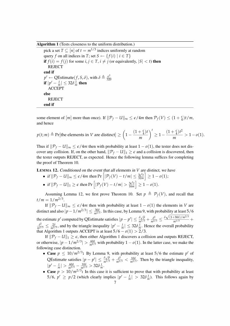
Algorithm 1 (Tests closeness to the uniform distribution.)pick a set T ⊆ [n] of t = m1/3 indices uniformly at randomquery f on all indices in T; set S← f (i) | i ∈ Tif f (i) = f (j) for some i, j ∈ T, i 6= j (or equivalently, |S| < t) then

REJECTend ifp′ ← QEstimate( f , S, δ), with δ , ε2

320if |p′ − t

m | ≤ 32δ tm then

ACCEPTelse

REJECTend if

some element of [m] more than once). If ‖P f −U‖∞ ≤ ε/4m then P f (V) ≤ (1 + ε4 )t/m,

and hence

p(t; m) , Pr[the elements in V are distinct] ≥(

1−(1 + ε

4 )tm

)t

≥ 1−(1 + ε

4)t2

m> 1− o(1).

Thus if ‖P f −U‖∞ ≤ ε/4m then with probability at least 1− o(1), the tester does not dis-cover any collision. If, on the other hand, ‖P f −U‖1 ≥ ε and a collision is discovered, thenthe tester outputs REJECT, as expected. Hence the following lemma suffices for completingthe proof of Theorem 10.

LEMMA 12. Conditioned on the event that all elements in V are distinct, we have• if ‖P f −U‖∞ ≤ ε/4m then Pr

[|P f (V)− t/m| ≤ 3ε2t

32m

]≥ 1− o(1);

• if ‖P f −U‖1 ≥ ε then Pr[|P f (V)− t/m| > 3ε2t

16m

]≥ 1− o(1).

Assuming Lemma 12, we first prove Theorem 10. Set p , P f (V), and recall thatt/m = 1/m2/3.

If ‖P f −U‖∞ ≤ ε/4m then with probability at least 1− o(1) the elements in V aredistinct and also |p− 1/m2/3| ≤ 30δ

m2/3 . In this case, by Lemma 9, with probability at least 5/6

the estimate p′ computed by QEstimate satisfies |p− p′| ≤ δ√

pm1/3 + δ2

m2/3 ≤δ√

(1+30δ)/m2/3

m1/3 +δ2

m2/3 ≤ 2δm2/3 , and by the triangle inequality |p′ − t

m | ≤ 32δ tm . Hence the overall probability

that Algorithm 1 outputs ACCEPT is at least 5/6− o(1) > 2/3.If ‖P f −U‖1 ≥ ε, then either Algorithm 1 discovers a collision and outputs REJECT,

or otherwise, |p− 1/m2/3| > 60δm2/3 with probability 1− o(1). In the latter case, we make the

following case distinction.• Case p ≤ 10/m2/3: By Lemma 9, with probability at least 5/6 the estimate p′ of

QEstimate satisfies |p− p′| ≤ δ√

pm1/3 + δ2

m2/3 < 10δm2/3 . Then by the triangle inequality,

|p′ − tm | >

60δm2/3 − 10δ

m2/3 > 32δ tm .

• Case p > 10/m2/3: In this case it is sufficient to prove that with probability at least5/6, p′ ≥ p/2 (which clearly implies |p′ − t

m | > 32δ tm ). This follows again by

7

Lemma 9, since p > 10/m2/3 implies δ√

pm1/3 + δ2

m2/3 ≤ p/2.So the overall probability that Algorithm 1 outputs REJECT is at least 5/6− o(1) > 2/3.

PROOF. [of Lemma 12] Let W f (V) = ∑y∈V P f (y). Assuming that all elements in Vare distinct, P f (V) = W f (V). For the first item of the lemma, it suffices to prove that if‖P f −U‖∞ ≤ ε/4m then

Pr[|W f (V)− t

m| > 3ε2t

32m

]≤ o(1)

and for the second item of the lemma, it suffices to prove that if ‖P f −U‖1 ≥ ε then

Pr[W f (V) > (1 +

3ε2

16)

tm

]≥ 1− o(1).

Note that the standard concentration inequalities cannot be used for proving the last inequalitydirectly, because the probabilities of certain elements underP f can be very high. To overcomethis problem, we define P f (y) , min3/m,P f (y) and W f (V) , ∑y∈V P f (y). Clearly

W f (V) ≤ W f (V) for any V, hence proving Pr[W f (V) > (1 + 3ε2

16 ) tm

]≥ 1 − o(1) is

sufficient. Surprisingly, this turns out to be easier:

LEMMA 13. The following three statements hold1. if ‖P f −U‖∞ ≤ ε/4m, then t

m ≤ E[W f (V)] <(

1 + ε2

16

)tm

2. if ‖P f −U‖1 ≥ ε, then E[W f (V)] >(

1 + ε2

4

)tm ;

3. Pr[∣∣∣W f (V)−E[W f (V)]

∣∣∣ > ε2t32m

]= o(1).

Assuming Lemma 13 we have:• if ‖P f −U‖∞ ≤ ε/4m then clearly W f (V) = W f (V), therefore

Pr[|W f (V)− t

m| > 3ε2t

32m

]≤ Pr

[∣∣∣W f (V)−E[W f (V)]∣∣∣ >

ε2t32m

]= o(1);

• if ‖P f −U‖1 ≥ ε then

Pr[

W f (V) < (1 +3ε2

16)

tm

]≤ Pr

[W f (V) < (1 +

3ε2

16)

tm

]≤ Pr

[∣∣∣W f (V)−E[W f (V)]∣∣∣ >

ε2t16m

]≤ Pr

[∣∣∣W f (V)−E[W f (V)]∣∣∣ >

ε2t32m

]= o(1).

Hence Lemma 12 follows. The proof of Lemma 13 is more technical, and it appears inAppendix B.

3.2 Testing Closeness to a Known Distribution

In this section we prove Theorem 1 based on Theorem 10. Let P f be an unknown distributionand let Pg be a known distribution, defined by f , g : [n] → [m] respectively. We show that

8

for any ε > 0, Algorithm 2 makes O(m1/3 log2 m log log mε5 ) queries and distinguishes the case

‖P f −Pg‖1 = 0 from the case ‖P f −Pg‖1 > 5ε with probability at least 2/3, satisfyingthe requirements of Theorem 1.§

Algorithm 2 (Tests closeness to a known distribution.)

1: letM , M0, . . . , Mk ← Bucket(Pg, [m], ε4 ) for k = 2 log m

log(1+ε/4)2: for i = 1 to k do3: if Pg(Mi) ≥ ε/k then4: if ‖(P f )|Mi

−U|Mi‖1 ≥ ε (check using the amplified version of Algorithm 1 from

Corollary 11) then5: REJECT6: end if7: end if8: end for9: if ‖(P f )〈M〉 − (Pg)〈M〉‖1 > ε/4 (check classically with O(

√k) = O(log m) queries

[7]) then10: REJECT11: end if12: ACCEPT

Observe that no queries are made by Algorithm 2 itself, and the total number of queries

made by calls to Algorithm 1 is bounded by k ·O( kε ·

m1/3 log log mε2 )+O(

√k) = O(m1/3 log2 m log log m

ε5 ).¶

In addition, the failure probability of Algorithm 1 is at most 1/ log2 m 1/k, so we canassume that with high probability none of its executions failed.

For any i ∈ [k] and any x ∈ Mi, by the definition of the buckets (1+ε/4)i−1

m log m ≤ Pg(x) ≤(1+ε/4)i

m log m . Thus, for any i ∈ [k] and x ∈ Mi, (1− ε4)/|Mi| < 1/(1 + ε

4 )|Mi| < (Pg)|Mi(x) <

(1 + ε4)/|Mi|, or equivalently for any i ∈ [k] we have ‖(Pg)|Mi

−U|Mi‖∞ ≤ ε

4|Mi | . Thismeans that if ‖P f −Pg‖1 = 0 then

1. for any i ∈ [k], ‖(P f )|Mi−U|Mi

‖∞ ≤ ε4|Mi | and thus the tester never outputs REJECT

in Line 5 (since we assumed that Algorithm 1 did not err in any of its executions).2. ‖(P f )〈M〉 − (Pg)〈M〉‖1 = 0, and hence the tester does not output REJECT in Line 10

either.On the other hand, if ‖P f −Pg‖1 > 5ε then by Corollary 8 we know that either

|(P f )〈M〉 − (Pg)〈M〉| > ε/4 or there is at least one i ∈ [k] for which P f (Mi) ≥ ε/kand ‖(P f )|Mi

− (Pg)|Mi‖1 > 5ε/4 (otherwise ‖P f −Pg‖1 must be smaller than 2(5ε/4 +

ε/4 + ε) = 5ε). In the first case the tester will reject in Line 10. In the second case the testerwill reject in Line 5 as ‖(P f )|Mi

− (Pg)|Mi‖1 > 5ε/4 implies (by the triangle inequality)

‖(P f )|Mi−U|Mi

‖1 > ε, since ‖(Pg)|Mi−U|Mi

‖1 < ε/4 by Lemma 6.

§We use 5ε instead ε for better readability in the sequel.¶The additional factor of k

ε is for executing Algorithm 1 on the conditional distributions (P f )|Mi, with

P f (Mi) ≥ εk .

9

4 Proof of Theorem 4

4.1 Quantum Upper Bound

The quantum tester is very simple, and completely based on existing ideas. First, run a variantof Shor’s algorithm to find the period of f (if there is one), using O(1) queries. Second, testwhether the purported period is indeed the period, using another O(1) queries as describedabove. Accept iff the latter test accepts.

For the sake of completeness we sketch here how Shor’s algorithm can be used to find theunknown period p of an f that is promised to be 1-1-p-periodic for some value of p ≤

√n/2.

Here is the algorithm:‖

1. First prepare the 2-register quantum state1√n ∑

i∈[n]|i〉|0〉

2. Query f once (in superposition), giving1√n ∑

i∈[n]|i〉| f (i)〉

3. Measure the second register, which gives some f (s) for s ∈ [p] and collapses the first

register to the i having the same f -value:1√bn/pc ∑

i∈[n],i=s mod p|i〉| f (i)〉

4. Do a quantum Fourier transform∗∗ on the first register and measure.Some analysis shows that with high probability the measurement gives an i such that∣∣∣∣ in− c

p

∣∣∣∣ <1

2n, where c is a random (essentially uniform) integer in [p]. Using con-

tinued fraction expansion, we can then calculate the unknown fraction c/p from theknown fraction i/n.††

5. Doing the above 4 steps k times gives fractions c1/p, . . . , ck/p, each given as a numer-ator and a denominator (in lowest terms). Each of the k denominators divides p, andif k is a sufficiently large constant then with high probability (over the ci’s), their leastcommon multiple is p.

4.2 Classical Lower Bound

We saw above that quantum computers can efficiently test 1-1-PERIODICITY P√n/4,√

n/2.Here we will show that this is not the case for classical testers: those need roughly

√r queries

for 1-1-periodicity testing Pr/2,r, in particular roughly n1/4 queries for r =√

n/2. Our proof

‖For this to work, the 1-1 property on [p] is crucial; for instance, quantum algorithms need about√

n queriesto find the period of functions with range 0, 1. Also the fact that p = O(

√n) is important, because the quantum

algorithm needs to see many repetitions of the period on the domain [n].∗∗This is the unitary map |x〉 → 1√

n ∑y∈[n] e2πixy/n|y〉. If n is a power of 2 (which we can assume here

without loss of generality), then the QFT can be implemented using O((log n)2) elementary quantum gates [31,Section 5.1].

††Two distinct fractions each with denominator≤√

n/2 are at least 4/n apart. Hence there is only one fractionwith denominator at most

√n/2 within distance 2/n from the known fraction i/n. This unique fraction can only

be c/p, and CFE efficiently finds it for us. Note that we do not obtain c and p separately, but just their ratio givenas a numerator and a denominator in lowest terms. If c and p were coprime that would be enough, but that neednot happen with high probability.

10

follows along the lines of Lachish and Newman [30]. However, since their proof applies tofunctions with range 0/1 that need not satisfy the 1-1 property, some modifications are needed.

Fix a sufficiently large even integer r < n/2. We will use Yao’s principle, proving alower bound for deterministic query testers with error probability≤ 1/3 in distinguishing twodistributions, one on negative instances and one on positive instances. First, the “negative”distribution DN is uniform on all f : [n] → [m] that are ε-far from Pr/2,r. Second, the“positive” distribution DP chooses a prime period p ∈ [r/2, r] uniformly, then chooses a 1-1function [p] → [m] uniformly (equivalently, chooses a sequence of p distinct elements from[m]), and then completes f by repeating this period until the domain [n] is “full”. Note thatthe last period will not be completed if p 6 |n.

Suppose q = o(√

r/ log r log n) is the number of queries of our deterministic tester.Fix a set Q = i1, . . . , iq ⊆ [n] of q queries. Let f (Q) ∈ [m]q denote the concatenatedanswers f (i1), . . . , f (iq). We prove two lemmas, one for the negative and one for the positivedistribution, showing f (Q) to be close to uniformly distributed in both cases.

LEMMA 14. For all η ∈ [m]q, we have PrDN [ f (Q) = η] = (1± o(1))m−q.

PROOF. We first upper bound the number of functions f : [n] → [m] that are ε-close top-periodic for a specific p. The number of functions that are perfectly p-periodic is mp, sincesuch a function is determined by its first p values. The number of functions ε-close to a fixedf is at most ( n

εn)mεn. Hence the number of functions ε-close to Pp is at most mp( nεn)mεn.

Therefore, under the uniform distribution U on all mn functions f : [n]→ [m], the probabilitythat there is a period p ≤ r for which f is ε-close to Pp is at most

r ·mr( nεn)mεn

mn ≤ mn/2+H(ε)n/ log m+εn−n,

where we used r < n/2, n ≤ m, and ( nεn) ≤ 2H(ε)n with H(·) denoting binary entropy. If

ε is a sufficiently small constant, then this probability is o(m−q) (in fact much smaller thanthat). Hence the variation distance between DN and the uniform distribution U is o(m−q),and we have∣∣∣∣Pr

DN[ f (Q) = η]−m−q

∣∣∣∣ =∣∣∣∣PrDN

[ f (Q) = η]− PrU

[ f (Q) = η]∣∣∣∣ = o(m−q).

LEMMA 15. There exists an event B such that PrDP [B] = o(1), and for all η ∈ [m]q withdistinct coordinates, we have PrDP [ f (Q) = η | B] = (1± o(1))m−q.

PROOF. The distribution DP uniformly chooses a prime period p ∈ [r/2, r]. By theprime number theorem (assuming r is at least a sufficiently large constant, which we may dobecause the lower bound is trivial for constant r), the number of distinct primes in this intervalis asymptotically

rln(r)

− r/2ln(r/2)

≥ r2 log r

.

Let B be the event that a p is chosen for which there exist distinct i, j ∈ Q satisfying i = j modp (equivalently, p divides i − j). For each fixed i, j there are at most log n primes dividing

11

i− j. Hence at most (q2) log n = o(r/ log r) p’s out of the at least r/2 log r possible p’s can

cause event B, implying PrDP [B] = o(1).Conditioned on B not happening, f (Q) is a uniformly random element of [m]q with

distinct coordinates, hence for each η ∈ [m]q with distinct coordinates we have

PrDP

[ f (Q) = η | B] =1m

1m− 1

· · · 1m− q + 1

= m−qq−1

∏i=0

(1 +

im− i

)= (1 + o(1))m−q.

Since (1− o(1))mq of all η ∈ [m]q have distinct coordinates, their weight under DPsums to 1− o(1), and the other possible η comprise only a o(1)-fraction of the overall weight.The query-answers f (Q) are the only access the algorithm has to the input. Hence the previ-ous two lemmas imply that an algorithm with o(

√r/ log r log n) queries cannot distinguish

DP and DN with probability better than 1/2 + o(1). This establishes the claimed classicallower bound.

5 Summary and Open ProblemsIn this paper we studied and compared the quantum and classical query complexities of anumber of testing problems. The first problem is deciding whether two probability distribu-tions on a set [m] are equal or ε-far. Our main result is a quantum tester for the case whereone of the two distributions is known (i.e., given explicitly) while the other is unknown andrepresented by a function that can be queried. Our tester uses roughly m1/3 queries to thefunction, which is essentially optimal. It would be very interesting to extend this quantumupper bound to the case where both distributions are unknown. Such a quantum tester wouldshow that the known-unknown and unknown-unknown cases have the same complexity inthe quantum world. In contrast, they are known to have different complexities in the classi-cal world: about m1/2 queries for the known-unknown case and about m2/3 queries for theunknown-unknown case. The classical counterparts of these tasks play an important role inmany problems related to property testing. We already mentioned one example, the graphisomorphism problem, where distribution testers are used as a black-box. We hope that thequantum analogues developed here and in [11] will find similar use.

The second testing problem is deciding whether a given function f : [n] → [m] isperiodic or far from periodic. For the specific version of the problem that we considered(where in the first case the period is at most about

√n, and the function is injective within

each period), we proved that quantum testers need only a constant number of queries (usingShor’s algorithm), while classical algorithms need about n1/4 queries. Both this result andAaronson’s recent result on “Fourier checking” [1] contrast with the constant-vs-log n andlog n-vs-

√n separations obtained by Buhrman et al. [13] for other testing problems, but still

leave open their question: is there a testing problem where the separation is “maximal”, in thesense that quantum testers need only O(1) queries while classical testers need Ω(n)?

Acknowledgements

We thank Avinatan Hassidim, Harry Buhrman and Prahladh Harsha for useful discussions,Frederic Magniez for a reference to [21], Pranab Sen for a reference to [26, 25], and Scott

12

Aaronson for pointing out that his Fourier checking result in [1] was the first constant-vs-polynomial quantum speed-up in property testing.

References

[1] S. Aaronson. BQP and the Polynomial Hierarchy. In Proceedings of 42nd ACM STOC,2010. arXiv:0910.4698.

[2] S. Aaronson and Y. Shi. Quantum lower bounds for the collision and the element dis-tinctness problems. Journal of the ACM, 51(4):595–605, 2004.

[3] A. Ambainis. Polynomial degree and lower bounds in quantum complexity: Collisionand element distinctness with small range. Theory of Computing, 1(1):37–46, 2005.quant-ph/0305179.

[4] A. Ambainis. Quantum walk algorithm for element distinctness. SIAM Journal onComputing, 37(1):210–239, 2007. Earlier version in FOCS’04. quant-ph/0311001.

[5] A. Ambainis, A. Childs, B. Reichardt, R. Spalek, and S. Zhang. Any AND-OR formulaof size n can be evaluated in time N1/2+o(1) on a quantum computer. In Proceedings of48th IEEE FOCS, 2007.

[6] A. Atici and R. Servedio. Quantum algorithms for learning and testing juntas. QuantumInformation Processing, 6(5):323–348, 2009.

[7] T. Batu, L. Fortnow, E. Fischer, R. Kumar, R. Rubinfeld, and P. White. Testing randomvariables for independence and identity. In Proceedings of 42nd IEEE FOCS, pages442–451, 2001.

[8] T. Batu, L. Fortnow, R. Rubinfeld, W. D. Smith, and P. White. Testing that distributionsare close. In Proceedings of 41st IEEE FOCS, pages 259–269, 2000.

[9] M. Blum, M. Luby, and R. Rubinfeld. Self-testing/correcting with applications to nu-merical problems. Journal of Computer and System Sciences, 47(3):549–595, 1993.Earlier version in STOC’90.

[10] G. Brassard, P. Høyer, M. Mosca, and A. Tapp. Quantum amplitude amplification andestimation. In Quantum Computation and Quantum Information: A Millennium Volume,volume 305 of AMS Contemporary Mathematics Series, pages 53–74. 2002. quant-ph/0005055.

[11] S. Bravyi, A. Hassidim, and A. Harrow. Quantum algorithms for testing propertiesof distributions. In Proceedings of 27th Annual Symposium on Theoretical Aspects ofComputer Science (STACS’2010), 2010. abs/0907.3920.

[12] H. Buhrman, R. Cleve, and A. Wigderson. Quantum vs. classical communicationand computation. In Proceedings of 30th ACM STOC, pages 63–68, 1998. quant-ph/9802040.

[13] H. Buhrman, L. Fortnow, I. Newman, and H. Rohrig. Quantum property testing. InProceedings of 14th ACM-SIAM SODA, pages 480–488, 2003. quant-ph/0201117.

[14] H. Buhrman and R. d. Wolf. Complexity measures and decision tree complexity: Asurvey. Theoretical Computer Science, 288(1):21–43, 2002.

[15] A. Childs and Y.-K. Liu. Quantum algorithms for testing bipartiteness and expansion ofbounded-degree graphs. Manuscript, Oct 22, 2009.

13

[16] R. Cleve, W. v. Dam, M. Nielsen, and A. Tapp. Quantum entanglement and the commu-nication complexity of the inner product function. In Proceedings of 1st NASA QCQCconference, volume 1509 of Lecture Notes in Computer Science, pages 61–74. Springer,1998. quant-ph/9708019.

[17] D. Deutsch and R. Jozsa. Rapid solution of problems by quantum computation. InProceedings of the Royal Society of London, volume A439, pages 553–558, 1992.

[18] E. Farhi, J. Goldstone, and S. Gutmann. A quantum algorithm for the HamiltonianNAND tree. Theory of Computing, 4(1):169–190, 2008. quant-ph/0702144.

[19] E. Fischer. The art of uninformed decisions. Bulletin of the EATCS, 75:97, 2001.[20] E. Fischer and A. Matsliah. Testing graph isomorphism. SIAM Journal on Computing,

38(1):207–225, 2008.[21] K. Friedl, F. Magniez, M. Santha, and P. Sen. Quantum testers for hidden group proper-

ties. Fundamenta Informaticae, 91(2):325–340, 2009. Earlier version in MFCS’03.[22] O. Goldreich, S. Goldwasser, and D. Ron. Property testing and its connection to learning

and approximation. Journal of the ACM, 45(4):653–750, 1998.[23] O. Goldreich and D. Ron. On testing expansion in bounded-degree graphs. Electronic

Colloquium on Computational Complexity (ECCC), 7(20), 2000.[24] L. K. Grover. A fast quantum mechanical algorithm for database search. In Proceedings

of 28th ACM STOC, pages 212–219, 1996. quant-ph/9605043.[25] L. Hales. The Quantum Fourier Transform and Extensions of the Abelian Hidden

Subgroup Problem. PhD thesis, University of California, Berkeley, 2002. quant-ph/0212002.

[26] L. Hales and S. Hallgren. An improved quantum Fourier transform algorithm and appli-cations. In Proceedings of 41st IEEE FOCS, pages 515–525, 2000.

[27] A. S. Holevo. Bounds for the quantity of information transmitted by a quantum commu-nication channel. Problemy Peredachi Informatsii, 9(3):3–11, 1973. English translationin Problems of Information Transmission, 9:177–183, 1973.

[28] Y. Inui and F. Le Gall. Quantum property testing of group solvability. In Proceedings of8th LATIN, pages 772–783, 2008.

[29] S. Kutin. Quantum lower bound for the collision problem with small range. Theory ofComputing, 1(1):29–36, 2005. quant-ph/0304162.

[30] O. Lachish and I. Newman. Testing periodicity. Algorithmica, 2009. Earlier version inRANDOM’05.

[31] M. A. Nielsen and I. L. Chuang. Quantum Computation and Quantum Information.Cambridge University Press, 2000.

[32] D. Ron. Property testing: A learning theory perspective. Foundations and Trends inMachine Learning, 1(3):307–402, 2008.

[33] P. W. Shor. Polynomial-time algorithms for prime factorization and discrete logarithmson a quantum computer. SIAM Journal on Computing, 26(5):1484–1509, 1997. Earlierversion in FOCS’94. quant-ph/9508027.

[34] D. Simon. On the power of quantum computation. SIAM Journal on Computing,26(5):1474–1483, 1997. Earlier version in FOCS’94.

[35] P. Valiant. Testing symmetric properties of distributions. In Proceedings of 40th ACMSTOC, pages 383–392, 2008.

14

A Quantum Queries and Approximate Counting – Proof ofLemma 9

Recall that the function f is assumed to be accessible by the oracle unitary transformation O f ,which acts on a (log n + log m)-qubit space by sending the basis vector |x〉|b〉 to |x〉|b ⊕f (x)〉 where ⊕ is bitwise addition modulo two.

For any set S ⊆ [m], let USf denote the unitary transformation which maps |x〉|b〉 to

|x〉|b ⊕ 1〉 if f (x) ∈ S, and to |x〉|b ⊕ 0〉 otherwise. This unitary transformation can beeasily implemented using log m ancilla bits and two queries to O f .‡‡ If fS : [n] → 0, 1is defined as fS(x) = 1 if and only if f (x) ∈ S, then the unitary transformation US

f acts asan oracle to the function fS. Brassard, Høyer, Mosca, and Tapp [10, Theorem 13] gave analgorithm to approximately count the size of certain sets.

THEOREM 16.[BHMT] For every positive integer q and ` > 1, and given quantum oracleaccess to a Boolean function h : [n] → 0, 1, there is an algorithm that makes q queries to

h and outputs an estimate t′ to t = |h−1(1)| such that |t′ − t| ≤ 2π`

√t(n−t)

q + π2`2 nq2 with

probability at least 1− 1/2(`− 1).

Lemma 9 follows easily from this theorem: PROOF. [of Lemma 9] The algorithm isbasically required to estimate | f−1

S (1)|. Using two queries to the oracle O f we can constructa unitary US

f that acts like an oracle for the Boolean function fS. Estimate t = | f−1S (1)| using

the algorithm in Theorem 16, with q = cm1/3/δ queries. Choosing c a sufficiently large

constant, with probability at least 5/6, the estimate t′ satisfies |t − t′| ≤ δ√

t(n−t)m1/3 + δ2n

m2/3 .Setting p′ = t′/n and bounding (n − t) with n we get that with probability at least 5/6,|p− p′| = |t−t′|

n ≤ δ√

pm1/3 + δ2

m2/3 .

B Proof of Lemma 13We start by computing the expected value of W f (V).

E[W f (V)] = ∑y∈V

∑z∈[m]P f (z)P f (z) = t

∑z:P f (z)<3/m

P f (z)2 + ∑z:P f (z)≥3/m

3P f (z)/m

= t

∑z∈[m]P f (z)2 − ∑

z:P f (z)≥3/mP f (z)(P f (z)− 3/m)

.

Let δ(z) , P f (z)− 1/m and let r , |z | δ(z) < 2/m|. Then

E[W f (V)] = t

(∑

z∈[m](1/m + δ(z))2 − ∑

z:δ(z)≥2/m(1/m + δ(z))(δ(z)− 2/m)

)

‡‡We need two queries to f instead of one, because the quantum algorithm has to “uncompute” the first queryin order to clean up its workspace.

15

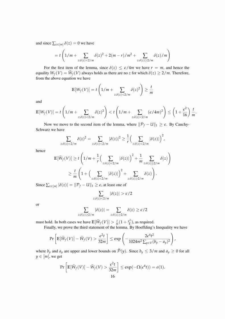
and since ∑z∈[m] δ(z) = 0 we have

= t

(1/m + ∑

z:δ(z)<2/mδ(z)2 + 2(m− r)/m2 + ∑

z:δ(z)≥2/mδ(z)/m

)

For the first item of the lemma, since δ(z) ≤ ε/4m we have r = m, and hence theequality W f (V) = W f (V) always holds as there are no z for which δ(z) ≥ 2/m. Therefore,from the above equation we have

E[W f (V)] = t

(1/m + ∑

z:δ(z)<2/mδ(z)2

)≥ t

m

and

E[W f (V)] = t

(1/m + ∑

z:δ(z)<2/mδ(z)2

)< t

(1/m + ∑

z:δ(z)<2/m(ε/4m)2

)≤(

1 +ε2

16

)tm

.

Now we move to the second item of the lemma, where ‖P f −U‖1 ≥ ε. By Cauchy-Schwarz we have

∑z:δ(z)<2/m

δ(z)2 = ∑z:δ(z)<2/m

|δ(z)|2 ≥ 1r

(∑

z:δ(z)<2/m|δ(z)|

)2,

hence

E[W f (V)] ≥ t

(1/m +

1r

(∑

z:δ(z)<2/m|δ(z)|

)2+

1m ∑

z:δ(z)≥2/mδ(z)

)

≥ tm

(1 +

(∑

z:δ(z)<2/m|δ(z)|

)2+ ∑

z:δ(z)≥2/mδ(z)

).

Since ∑z∈[m] |δ(z)| = ‖P f −U‖1 ≥ ε, at least one of

∑z:δ(z)<2/m

|δ(z)| > ε/2

or∑

z:δ(z)≥2/m|δ(z)| = ∑

z:δ(z)≥2/mδ(z) ≥ ε/2

must hold. In both cases we have E[W f (V)] > tm (1 + ε2

4 ), as required.Finally, we prove the third statement of the lemma. By Hoeffding’s Inequality we have

Pr[

E[W f (V)]− W f (V) >ε2t

32m

]≤ exp

(− 2ε4t2

1024m2 ∑y∈V(by − ay)2

),

where by and ay are upper and lower bounds on P(y). Since by ≤ 3/m and ay ≥ 0 for ally ∈ [m], we get

Pr[

E[W f (V)]− W f (V) >ε2t

32m

]≤ exp(−Ω(ε4t)) = o(1).

16

C Proof of Theorem 3

In [20], the bottleneck (with respect to the query complexity) of the algorithm for testing graphisomorphism in the known-unknown case is the subroutine that tests closeness between twodistributions over V. All other parts of the algorithm make only a polylogarithmic numberof queries. Therefore, our main theorem implies that with quantum oracle access, graphisomorphism in the known-unknown setting can be tested with O(|V|1/3) queries.

On the other hand, a general lower bound on the query complexity of testing distributionsin the known-unknown case need not imply a lower bound for testing graph isomorphism. Butstill, in [20] it is proved that a lower bound on the query complexity for deciding whether thefunction f : [n] → [n] is one-to-one (that is injective) or is two-to-one (that is pre-imageof any j ∈ [n] is either empty or size 2) is sufficient for showing a matching lower boundfor graph isomorphism. Since our quantum lower bound for the known-unknown testing caseis derived from exactly that problem (see Appendix D), we get a matching lower bound ofΩ(|V|1/3) on the number of quantum queries necessary for testing graph isomorphism in theknown-unknown case.

For the unknown-unknown case, the lower bound mentioned in Theorem 3 follows fromthe lower bound for the known-unknown case. To get the upper bound of O(|V|7/6) queries,we have to slightly modify the algorithm from [20]. We start by outlining the ideas in thealgorithm of [20] for testing isomorphism between two unknown graphs G and H.

Let G be a graph and CG ⊆ V(G). A CG-label of a vertex v ∈ V(G) is a binary vectorof length |CG| that represents the neighbors of v in CG. The distribution PCG over 0, 1|CG |

is defined according to the graph G, where for every x ∈ 0, 1|CG | the probability PCG(x) isproportional to the number of vertices in G with CG-label equal to x. Notice that the supportof PCG is bounded by |V(G)|.

The algorithm of [20] is based on two main observations:1. if there is an isomorphism σ between G and H, then for every CG ⊆ V(G) and the

corresponding CH , σ(CG), the distributions PCG and PCH are identical.2. if G and H are far from being isomorphic, then for every equally-sized (and not too

small) CG ⊆ V(G) and CH ⊆ V(H), either the distributions PCG and PCH are far, orotherwise it is possible to “realize” with only a poly-logarithmic number of queries thatthere exists no isomorphism that maps CG to CH.

Once these observations are made, the high level idea in the algorithm of [20] is to go overa sequence of pairs of sets CG, CH (such that with high probability at least one of them sat-isfies CH , σ(CG) if indeed an isomorphism σ exists), and to test closeness between thecorresponding distributions PCG and PCH .

This sequence of pairs is defined as follows: first we pick (at random) a set UG of|V|1/4 log3 |V| vertices from G and a set UH of |V|3/4 log3 |V| vertices from H. Thenwe make all |V|5/4 log3 |V| possible queries in UG × V(G). After this, for any CG ⊆ UGthe distribution PCG is known exactly. Indeed, the sequence of sets CG, CH will consist ofall pairs CG ⊆ UG, CH ⊆ UH , where both CG and CH are of size log2 |V|. It is not hardto prove that if G and H have an isomorphism σ, then with probability 1− o(1) the size ofUH ∩ σ(UG) will exceed log2 |V|, and hence one of the pairs will satisfy CH , σ(CG).

Now, for each pair CG, CH we test if the distributions PCG and PCH are identical. Since17

we know the distributions PCG (for every CG ⊆ UG), we only need to sample the distributionsPCH . Sampling the distributions PCH is done by taking a set S ⊆ V(H) of size O(

√|V|) and

re-using it for all these tests. In total, the algorithm in [20] makes roughly |UG × V(G)|+|UH × S| = O(|V|5/4) queries.

To get the desired improvement, we follow the same path, but use our quantum dis-tribution tester instead of the classical one. This allows us to reduce the size of the set Sto O(|V|1/3). Consequently, in order to balance the amount of queries we make in bothgraphs, we will resize the sets UG and UH to O(|V|1/6) and O(|V|5/6) respectively, whichstill satisfies the “large-intersection” property and brings the total number of queries down to|UG ×V(G)|+ |UH × S| = O(|V|7/6).

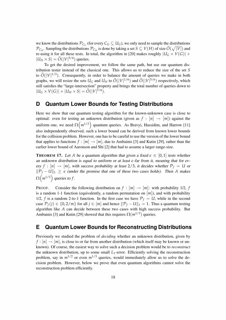
D Quantum Lower Bounds for Testing Distributions

Here we show that our quantum testing algorithm for the known-unknown case is close tooptimal: even for testing an unknown distribution (given as f : [n] → [m]) against the

uniform one, we need Ω(

m1/3)

quantum queries. As Bravyi, Hassidim, and Harrow [11]also independently observed, such a lower bound can be derived from known lower boundsfor the collision problem. However, one has to be careful to use the version of the lower boundthat applies to functions f : [m] → [m], due to Ambainis [3] and Kutin [29], rather than theearlier lower bound of Aaronson and Shi [2] that had to assume a larger range-size.

THEOREM 17. Let A be a quantum algorithm that given a fixed ε ∈ [0, 1] tests whetheran unknown distribution is equal to uniform or at least ε-far from it, meaning that for ev-ery f : [n] → [m], with success probability at least 2/3, it decides whether P f = U or‖P f −U‖1 ≥ ε (under the promise that one of these two cases holds). Then A makes

Ω(

m1/3)

queries to f .

PROOF. Consider the following distribution on f : [m] → [m]: with probability 1/2, fis a random 1-1 function (equivalently, a random permutation on [m]), and with probability1/2, f is a random 2-to-1 function. In the first case we have P f = U, while in the secondcase P f (j) ∈ 0, 2/m for all j ∈ [m] and hence ‖P f −U‖1 = 1. Thus a quantum testingalgorithm like A can decide between these two cases with high success probability. ButAmbainis [3] and Kutin [29] showed that this requires Ω(m1/3) queries.

E Quantum Lower Bounds for Reconstructing Distributions

Previously we studied the problem of deciding whether an unknown distribution, given byf : [n] → [m], is close to or far from another distribution (which itself may be known or un-known). Of course, the easiest way to solve such a decision problem would be to reconstructthe unknown distribution, up to some small L1-error. Efficiently solving the reconstructionproblem, say in m1/2 or even m1/3 queries, would immediately allow us to solve the de-cision problem. However, below we prove that even quantum algorithms cannot solve thereconstruction problem efficiently.

18

THEOREM 18. Let 0 < ε < 1/2 be a fixed constant. Let A be a quantum algorithm thatsolves the reconstruction problem, meaning that for every f : [n] → [m], with probability atleast 2/3, it outputs a probability distribution P ∈ [0, 1]m such that ‖P − P f ‖1 ≤ ε. ThenA makes Ω(m/ log m) queries to f .

PROOF. The proof uses some basic quantum information theory, and is most easily stated ina communication setting. Suppose Alice has a uniformly distributed m-bit string x of weightm/2. This is a random variable with entropy log ( m

m/2) = m − O(log m) bits. Let q bethe number of queries A makes. We will show below that Alice can give Bob Ω(m) bits ofinformation (about x), by a process that (interactively) communicates O(q log m) qubits. ByHolevo’s Theorem [27] (see also [16, Theorem 2]), establishing k bits of mutual informationrequires communicating at least k qubits, hence q = Ω(m/ log m).

Given an x ∈ 0, 1m of weight n = m/2, let f : [n]→ [m] be an injective function toj | xj = 1, and let P f be the corresponding probability distribution over m elements (whichis P f (j) = 2/m where xj = 1, and P f (j) = 0 where xj = 0). Let P be the distributionoutput by algorithm A on f . We have ‖P − P f ‖1 ≤ ε with probability at least 2/3. Definea string x ∈ 0, 1m by xj = 1 iff P(j) ≥ 1/m. Note that at each position j ∈ [m]where xj 6= xj, we have |P(j)− P f (j)| ≥ 1/m. Hence ‖P − P f ‖1 ≥ d(x, x)/m. Since‖P − P f ‖1 ≤ ε (with probability at least 2/3), the algorithm’s output allows us to produce(with probability at least 2/3) a string x ∈ 0, 1m at Hamming distance d(x, x) ≤ εm fromx. But then it is easy to calculate that the mutual information between x and x is Ω(m) bits.

Finally, to put this in the communication setting, note that Bob can run the algorithmA, implementing each query to f by sending the O(log n)-qubit query-register to Alice, whoplugs in the right answer and sends it back (this idea comes from [12]). The overall commu-nication is O(q log m) qubits.

F From Sampling Problems to Oracle ProblemsA standard way to access a probability distribution P on [m] is by sampling it: samplingonce gives the outcome y ∈ [m] with probability P(y). However, in this paper we usuallyassume that we can access the distribution by querying a function f : [n] → [m], where theprobability of y is now interpreted as the fraction of the domain that is mapped to y. Belowwe describe the connection between these two approaches.

Suppose we sample P n times, and estimate each probability P(y) by the fraction P(y)of times y occurs among the n outcomes. We will analyze how good an estimator this is forP(y). For all j ∈ [n], let Yj be the indicator random variable that is 1 if the jth sample is y, and0 otherwise. This has expectation E[Yj] = P(y) and variance Var[Yj] = P(y)(1−P(y)).Our estimator is P(y) = ∑j∈[n] Yj/n. This has expectation E[P(y)] = P(y) and varianceVar[P(y)] = P(y)(1− P(y))/n, since the Yj’s are independent. Now we can bound theexpected error of our estimator for P(y) by

E[|P(y)−P(y)|

]≤√

E[|P(y)−P(y)|2

]=√

Var[P(y)

]≤√P(y)/n.

And we can bound the expected L1-distance between the original distribution P and its ap-19

proximation P by

E[‖P − P‖1

]= ∑

y∈[m]E[|P(y)−P(y)|

]≤ ∑

y∈[m]

√P(y)/n ≤

√m/n,

where the last inequality used Cauchy-Schwarz and the fact that ∑y P(y) = 1. For in-stance, if n = 10000m then E[‖P − P‖1] ≤ 1/100, and hence (by Markov’s Inequality)‖P − P‖1 ≤ 1/10 with probability at least 9/10. If we now define a function f : [n]→ [m]by setting f (j) to the jth value in the sample, we have obtained a representation which isa good approximation of the original distribution. Note that if n = o(m) then we cannothope to be able to approximately represent all possible m-element distributions by somef : [n] → [m], since all probabilities will be integer multiples of 1/n. For instance ifP is uniform and n = o(m), then the total L1-distance between P and a P induced byany f : [n] → [m] is near-maximal. Accordingly, the typical case we are interested in isn = Θ(m).

20