New Models of the Economy and the Financial System Tsomocos.pdf · New Models of the Economy and...
39
New Models of the Economy and the Financial System Charles A.E. Goodhart and Dimitri P. Tsomocos Financial Markets Group, London School of Economics & Said Business School, University of Oxford The Macroprudential Toolkit: Measurement and Analysis Washington D.C. December 1-2, 2011 1
Transcript of New Models of the Economy and the Financial System Tsomocos.pdf · New Models of the Economy and...

New Models of the Economy
and
the Financial System
Charles A.E. Goodhart and Dimitri P. Tsomocos
Financial Markets Group, London School of Economics
&
Said Business School, University of Oxford
The Macroprudential Toolkit: Measurement and Analysis
Washington D.C.
December 1-2, 2011 1

Frictions and Default • Inability to commit
– Ex-post penalties for default allow for borrowing and
intertemporal smoothing
2
• Complete vs. Incomplete Markets
– If markets are complete and loan terms are comprehensive,
i.e. any penalty for default can be applied, then default can be
excluded and the Arrow-Debreu equilibrium is reached
– When markets are incomplete, allowing for positive default
in equilibrium can be welfare improving
• Optimizing financial institutions
– Improve hedging opportunities and consumption smoothing
among heterogeneous agents: offer and bridge different types
of lending and borrowing contracts

Externalities and Default • Deadweight loss of default: Price taking behavior can lead to
inefficient level of aggregate default and aggregate moral hazard
• Financial system acts as an amplifier of primitive shocks
– Drop in the supply of credit due to loan losses further suppresses prices
and income making default worse
– Default by financial institutions results in shocks being transferred
throughout the economy
• Endogenous default and general equilibrium
– Interaction between liquidity and default
– Distinct regulatory policies will affect incentives in different ways
– Externalities from relative price effects (constrained Pareto suboptimality)
– Macroprudential vs. microprudential regulation
3

A benchmark model
Financial Regulation in General Equilibrium Goodhart, Kashyap, Tsomocos & Vardoulakis (2011)
• General equilibrium
• Externalities from the financial system:
Default, credit crunches and fire sales
• Financial system that allows
– Regulatory arbitrage
– Various regulatory tools
• Liquidity and securitization
4

Our model ingredients
• Two goods: houses, potatoes
• One security (MBS)
• Timing, t=1 (no uncertainty), t=2 (G or B outcome)
• 3 types of households, which differ in endowments
– “R” (rich) endowed with lots of houses, present at t=1 & 2
– “P” (poorer) endowed with potatoes, present at t=1 & 2
– “F” (first time buyers) endowed with potatoes, present t=2
• 2 types of financial institution
– b (bank) high risk aversion and big balance sheet
– N (non-bank) low risk aversion
• CB (central bank) that makes short term loans to b
5
Model characteristics
• Only uncertainty is relative quantity of potatoes vs.
houses and the amount of monetary endowments
• Households try to smooth consumption across goods
within the period and total consumption over time
• Intermediaries improve smoothing but at the cost of
amplifying shocks
• Regulations damp amplification of shocks but restrict
smoothing 6

Externalities and tools
• Knock effects from house price collapse and
subsequent repo default
– Fire sale of MBS by banks
– Deposit defaults
– Potential margin spiral
– (Distortion also due to dead weight costs of default
that tilts consumption towards the good state)
• Five potential regulatory tools:
– Loan to value ratios, margin requirements, capital
ratio, liquidity ratio, dynamic provisioning
– Are they complements or substitutes, why?
7

Three channels of financial regulation
1) Ex-ante tools: Discourage initial lending to make the bust less
extreme
– Margin requirements on repos, loan-to-value requirements on
mortgages, potentially capital or liquidity requirements on banks
2) Shore up the banks in the event of a bust
– Insist on capital
– Liquidity requirement make fire sales worse
3) Lean against the boom
– Dynamic provisioning on real estate related credit
– Hard to use capital, loan-to-value or margin requirement
8
Some conclusions
• Modeling the frictions matters and there is a high payoff to
being precise about the failures of Modigliani-Miller
• Our analysis shows that focusing on the channels, through
which the regulatory tools operate, is probably more important
than the institutions or markets to which they are applied
• Conventional monetary policy affects the short end of the yield
curve, while regulatory policy intervenes at a different stage of
the transmission mechanism
• Multiple channels of instability require multiple tools
(Tinbergen rule), and just capital, or even just capital and
liquidity, are not likely to be sufficient 9

Why the boom is hard to regulate? • Haircuts on repo loans are endogenous and depend on the
prevailing expectations of the marginal buyer (Geanakoplos,
2003)
• Regulatory ratios which incorporate asset prices are high in the
upturn
• Bad news about the economic prospects deplete the equity of
the natural buyer and lead to a market/funding liquidity spiral
(Brunnermeier & Pedersen, 2008)
• In Bhattacharya et al. (2011) we focus on the build-up face of
risk and how agents shift their portfolios towards riskier assets
by increasing borrowing at low interest rates (Minsky’s
Financial Instability Hypothesis, 1992) 10

Expectations and Leverage ctd.
• Risk shifting may look efficient due to improved
expectations
• However, even in CAPM economies the ability to
default makes agents undertake higher downside risk
and invest in asset with suboptimal Sharpe ratios
• When they factor their impact on overall-not
marginal-default and borrowing rates, they switch to
the safer asset with a higher Sharpe ratio
• Unweighted leverage requirement can lead to internal
deleveraging by cutting lending to safer assets
11
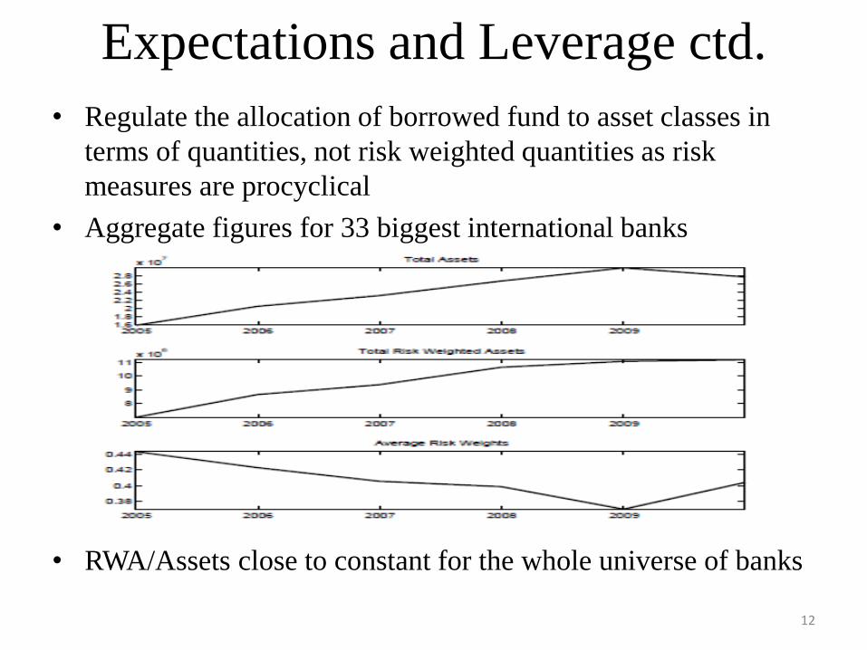
Expectations and Leverage ctd.
• Regulate the allocation of borrowed fund to asset classes in
terms of quantities, not risk weighted quantities as risk
measures are procyclical
• Aggregate figures for 33 biggest international banks
• RWA/Assets close to constant for the whole universe of banks
12

Dynamics • Martinez and Tsomocos (2011) take our overall
approach to dynamics and consider a model to
examine the interaction between liquidity and default
in a DSGE framework
• They conclude that liquidity and endogenous default
are indispensable parts of any measure of financial
stability
• Also, liquidity and default generate medium term
effects that are not captured by standard neo-
Keynesian models (Bernanke, Gertler and Gilchrist,
1999, Curdia and Woodford, 2009)
13

Overall
• We propose an approach that brings liquidity and
endogenous default in the center of macroeconomic
analysis
• Institutions and heterogeneity are important
• Model the micro-foundations of regulatory
interventions
• Propose a tractable framework to analyse monetary
and regulatory policy in an integrated model. 14
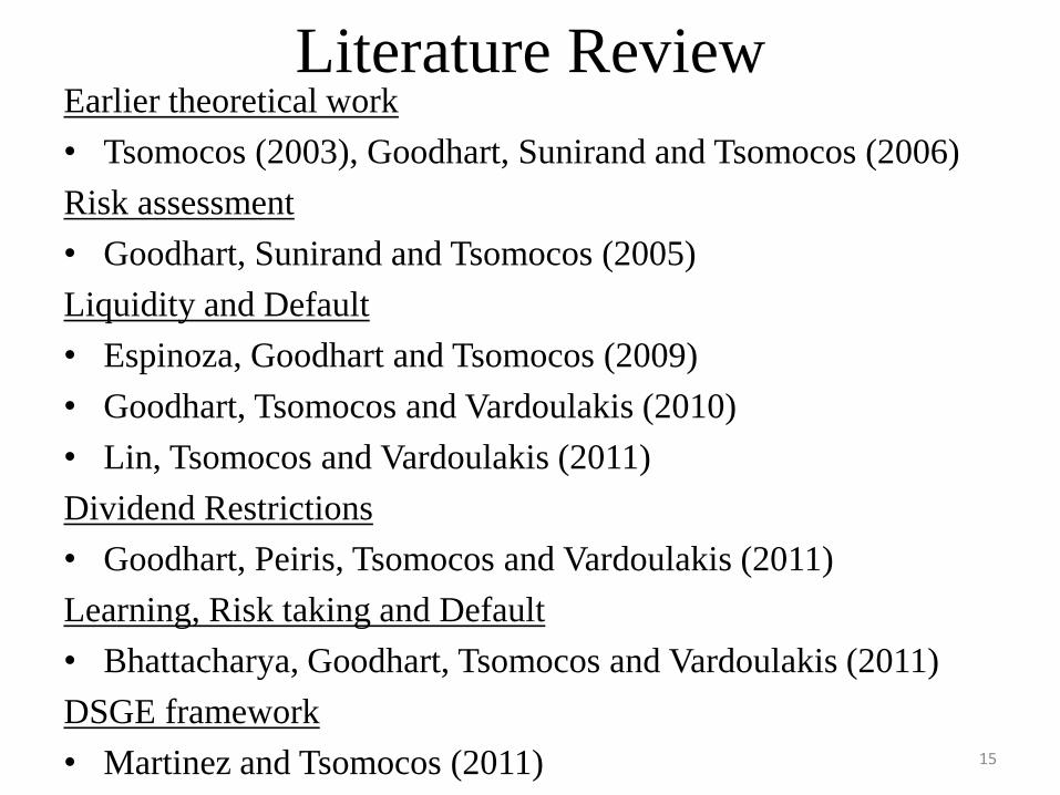
Literature Review Earlier theoretical work
• Tsomocos (2003), Goodhart, Sunirand and Tsomocos (2006)
Risk assessment
• Goodhart, Sunirand and Tsomocos (2005)
Liquidity and Default
• Espinoza, Goodhart and Tsomocos (2009)
• Goodhart, Tsomocos and Vardoulakis (2010)
• Lin, Tsomocos and Vardoulakis (2011)
Dividend Restrictions
• Goodhart, Peiris, Tsomocos and Vardoulakis (2011)
Learning, Risk taking and Default
• Bhattacharya, Goodhart, Tsomocos and Vardoulakis (2011)
DSGE framework
• Martinez and Tsomocos (2011) 15

Back-up Slides
for Goodhart, Kashyap,
Tsomocos, Vardoulakis
16

Household P’s budget constraints
17
1 1 1 1
1 1 1 1
2 2 2 2
2 2 2 2
2 2 2 2
(1 )
1
(1 )
P P P P
h h
P P
p p
P M P P P
gh gh g g
P P
g g gp gp
P P P
bh bh b b
P c E M B
B r P q
M P c E B
B r P q
P c E B
2 2 2 2 (1 )P P
b b bp bpB r P q
Housing constraint
Bridge loan repayment
Mortgage repayment and
additional housing rental
Bridge loan repayment
Mortgage default and
housing rental
Bridge loan repayment

Household F’s Optimization Problem
18
2 2 , 2 2 2 2
1 1
2 2 2 2
2 2 2 2
2 2 2 2
,
where
1 1,
1 1
and
(1 )
F F
P P P P P P
g gp gh b bp bh
F
p h p h
F F
F
F F F F
F
F
sh sh s s
F F
s s sp s
F
p
U c c U c c
U c c c c
P c E B
r P
U
B q
Housing rental
Bridge loan repayment

Household R’s Optimization Problem
19
1 1 2 2 1 2
2 2 1 2
1 1
, , , ,
1 1 1 1
1 1 1 1
2 2 2 2 2
, , 1
, 1
where
1 1 ,
1 1
(1 )
andR R
R R R R R R R R
p h g gp h gh
R R R R
b bp h bh
s p s h s p s hR
R R R R
p p
R R
h h
R R R D R
sp sp
R
s
R R
R
s s
R R
U c c U c c c
U c c c
U c c c c
P c D E B
B r P q
P c
U
E B V D
2 2 2 2
1
(1 )
D
R R
s s sh shB r P q
Potato purchase /deposit choice
Bridge loan repayment
Potatoes in period 2
Bridge loan repayment

Bank b’s Optimization Problem
20
__
1 2 2 2
1
1 1 1
11
1 1 1 1 1
_
and period 1 budget constrain
1 (1 )
where
1P
1ts
1 (1 )
re
D
s s s s
s
t
C
po
s ts
M
B
P P v D
L L CC E B D
M CC P M
B r cash
P
L r
Portfolio allocation
Securitization decision
CB repayment

Bank b’s Second Period Constraints
21
___
___
12 2 1 2 2 2 2
12 2 2 2 2 2
12 2 1 2 2
___
2 2
2 2 2 2 2
1
1 1 (1 ) 1 (1 )
1
1
D M
g g g g g g
M CB
g g g repo g g g
D M
b b b b b b
M
b b b b
repo
b
L v D cash E B P M M
L r L M M B r
L v D cash E B P M
L r V M
___
1 2 21 (1 )M CB
b bM B r
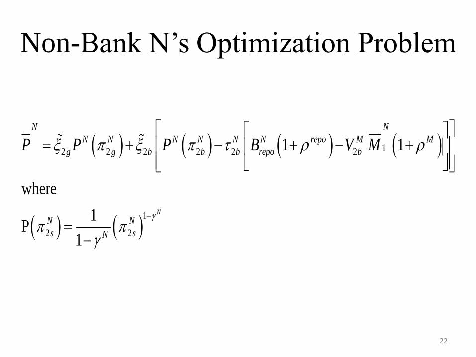
Non-Bank N’s Optimization Problem
22
12 2 2 2 2 2
1
2 2
__ ___
1 1
where
1P
1
N
N N
N N N N N N M M
g g b b b b
repo
repo
N N
Ns s
P P P B V M

Non-Bank N’s Budget Constraints
23
___
___
___ _
11 1
22 2
1 22
2
__
__
2 2
_
1 1
1
N
M N N
repo
N
M Nss s
N N
N M N repogg repo
N
N M Mbb b
P M E B
P M E
M M B
V M
MBS purchase in period 1
Cash in the market pricing
Capital gains minus repo
loan repayment
Default on the repo
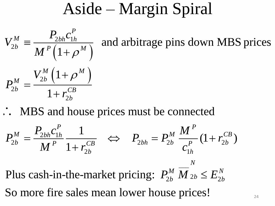
Aside – Margin Spiral
24
2 12
2
2
2
2 12 2 2 2
2 1
and arbitrage pins down MBS prices1
1
1
MBS and house prices must be connected
1 (1 )
1
Plus cash-in-the-market pricing
PM bh hb P M
M M
bM
b CB
b
P PM M CBbh hb bh b bP CB P
b h
P cV
M
VP
r
P c MP P P r
M r c
___
22 2
So more fire sales mean lower h
:
ouse prices!
N
M Nbb bP M E

Loan to Value and Haircut Regulation
25
1 1
1
1
_
1
__
(mortgage divided by house price value)
(N's equity relative to its borrowing)
PP
P
h h
NN
N
M
MLTV
P c
EMR
P M
Liquidity and Capital rules depend on point
in time when they are measured

b’s Middle of Period 1 Balance Sheet
26
1 1
1
1
1 1 1
1 1
L E
L
M - M D
r L B
r B
repo
CB
Assets Liabilities
11 1 1 1 1 1
___
( 1)CB Mr L r B P M

27
Liquidity and Capital Regulation
1 11
1
___
1 1
11 _
11
__
(riskless assets get zero risk weight)
re
mid
M repo
repo
m d
po
i
ECR
rw M M rw L
LLCR
L L M M
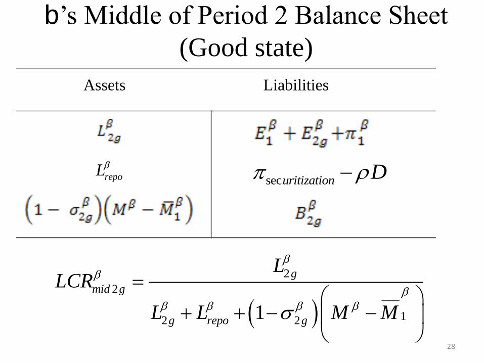
b’s Middle of Period 2 Balance Sheet
(Good state)
28
Assets Liabilities
__
2
2
12 2
_
1
g
mid g
g repo g
LLCR
L L M M
securitization D repoL
29
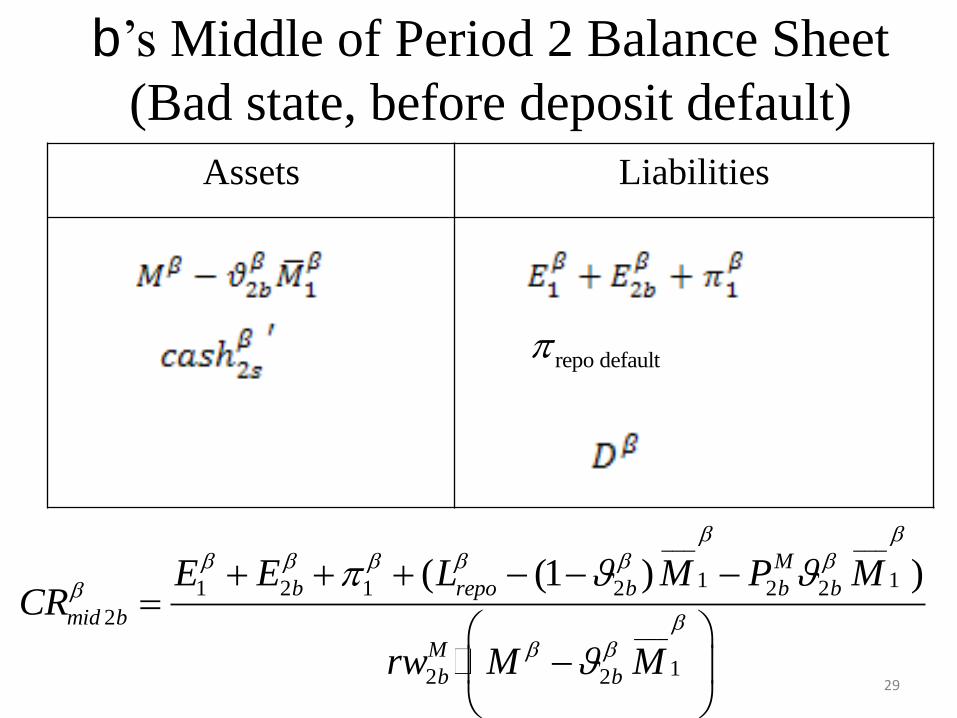
b’s Middle of Period 2 Balance Sheet
(Bad state, before deposit default)
Assets Liabilities
1
___ __
11 2 1 2 2 2
2
12
_
_
2
__
( (1 ) )repo
M
b b b b
mid b
M
b b
E E L M P MCR
rw M M
repo default

30
b’s Middle of Period 2 Balance Sheet
(Bad state, after deposit default) Assets Liabilities
22
12
___
2( )
bmid b
b b
LLCR
L M M
repo default

Dynamic Provisioning
31
2 2
1
2 2 2
11 2 2 2 2
___
Define Real Estate Related Credit Growth as
% 1 %
Provision per dollar of lending whenever g > "x"
1 % %
Makes
P F
g g
P P
D
gp gh g
M
g g g g
B Bg
M B
L L v D g x
cash E B P M M
it possible to lean against the boom without
directly distorting the allocations in the bust

Raising LTVs
1. T=1 reduces mortgage lending (and MBS which
raises mortgage rates)
2. T=2, bad state, raises mortgage repayment rate,
reduces deposit default rate, reduces fire sales
3. Mr. P and Mr. F worse off, Mr. R slightly better off,
raises utility for b and N (due to much higher MBS prices in the
good state and the larger spread between mortgage rates and deposit rates).
32
1 1
( ) P
P
P
h h
MLTV
P c

Raising haircuts
1. T=1, reduces repo borrowing, raises costs of
mortgages, total bank mortgages are higher
2. T=2, Reduces size of repo default, raises mortgage
repayment rate, and house prices
3. Mr P’s welfare is ambiguously affected, as is Mr.
R’s, but F is worse off. Raises utility for b and
slightly for N.
33
1
11
___( )
NN
N
M
EMR
P M

Raising Capital Requirements (middle of period 1)
1. T=1, reduces mortgage issuance, raises securitization
and raises the mortgage rate
2. T=2, less severe mortgage default, higher deposit
repayment
3. Mr P and Mr F are worse off, Mr. R hardly affected
4. b’s profits skewed towards period 1, with higher
utility, N’s profits and utility higher.
(Conjecture: Excess securitization only leads to perverse effects if
total mortgage credit is higher)
34
___
1 11
11 1
( )repo
rep
M
o
mid
ECR
rw M M rw L

Raising Capital Requirements (middle of period 2)
1. T=1, really reduces mortgage issuance, cuts
MBS and raises the mortgage rate
2. T=2, more bridge lending, less severe
mortgage default, higher deposit repayment
3. Mr P and Mr F are worse off, Mr. R hardly
affected. Raises utility for b and N. 35
1
___ ___
__
11 2 1 2 2 2
2
12 2
_
( (1 )(
) )
repo
M
b b b b
mid b
M
b b
E E L M P MCR
rw M M

Raising LCR (middle of period 1)
1. T=1, b reduces mortgages and MBS, raises the
mortgage rate, does more bridge lending
2. T=2, less severe mortgage default, higher deposit
repayment
3. Mr P’s is better off; Mr F is strictly worse off, Mr. R is
hardly affected. Massively raises utility for b and N.
(P gains from the easier bridge finance and lower default
costs)
36
11
1
_
1
__( )mid
repo
LLCR
L L M M

Raising LCR (middle of bad state)
1. T=1, b reduces mortgages and MBS (barely), lowers
the mortgage rate, does more bridge lending
2. T=2, forced fire sale, more severe mortgage default,
lower deposit repayment
3. Mr P’s is better off; Mr F is strictly worse off, Mr. R is
hardly affected. Lowers utility for b but raises it for N.
(Fire sale is the only way to comply with the regulation)
37
22
12
__
2
_( )
( )
bmid b
b b
LLCR
L M M

Dynamic Provisioning
38
2 2
1
Marginal cash requirement
% 1 % % 20({ {} })P F
g g
P P
B Bg x
M B
• k chosen so that incremental loans require 25 cents to be set aside
• Raises the cost of the mortgage loans in the boom
• Reduces the value of land in the boom, so raises the value of the
endowments for P & F They borrow more
• b also offers more credit in period 1
• F & P are better off, R, b and N worse off

Combo Regulation
• Marginal dynamic provisioning, marginal haircut
increase and 1% increase in capital requirements
• Switch from mortgage credit to more bridge lending
by the bank in period 1
• Fewer fire sales and higher deposit repayment in
period 2
• R gains due to small deposit losses
• P gains to smaller defaults and more housing
consumption in the boom
• (β better off and N worse off)
39