New Keynesian Model - James Murray · New Keynesian Model ECO 400: Monetary Theory and Policy ......
95
Static Model Dynamic Model New Keynesian Model ECO 400: Monetary Theory and Policy December 15, 2009 ECO 400: Monetary Theory and Policy New Keynesian Model
-
Upload
nguyenkhue -
Category
Documents
-
view
221 -
download
0
Transcript of New Keynesian Model - James Murray · New Keynesian Model ECO 400: Monetary Theory and Policy ......

Static ModelDynamic Model
New Keynesian Model
ECO 400: Monetary Theory and Policy
December 15, 2009
ECO 400: Monetary Theory and Policy New Keynesian Model

Static ModelDynamic Model
Goals of this chapter
Goals of this chapter 2/ 17
1 Learn shortcomings of the traditional IS/LM/AS model.
2 Understand a framework for endogenous monetary policy.
3 Learn a static model of inflation and output determination.
4 Learn how to pronounce Keynes. It’s like candy canes.
ECO 400: Monetary Theory and Policy New Keynesian Model

Static ModelDynamic Model
Background—Three EquationsGraphical Solution
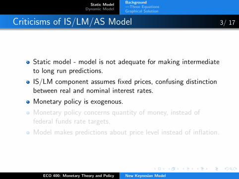
Criticisms of IS/LM/AS Model 3/ 17
Static model - model is not adequate for making intermediateto long run predictions.
IS/LM component assumes fixed prices, confusing distinctionbetween real and nominal interest rates.
Monetary policy is exogenous.
Monetary policy concerns quantity of money, instead offederal funds rate targets.
Model makes predictions about price level instead of inflation.
ECO 400: Monetary Theory and Policy New Keynesian Model

Static ModelDynamic Model
Background—Three EquationsGraphical Solution
Criticisms of IS/LM/AS Model 3/ 17
Static model - model is not adequate for making intermediateto long run predictions.
IS/LM component assumes fixed prices, confusing distinctionbetween real and nominal interest rates.
Monetary policy is exogenous.
Monetary policy concerns quantity of money, instead offederal funds rate targets.
Model makes predictions about price level instead of inflation.
ECO 400: Monetary Theory and Policy New Keynesian Model

Static ModelDynamic Model
Background—Three EquationsGraphical Solution
Basics of Model 4/ 17
Three equation model of three variables:1 Output gap: percentage difference between real GDP and
potential real GDP.2 Inflation rate: percentage growth rate in overall price level.3 Nominal interest rate: for simplicity assume one interest rate
= federal funds rate.
Very simple closed economy model with no investment,government spending (output = consumption).
IS curve: Microfounded equation of optimal consumptiondecisions combined with market clearing.
Phillips curve: Microfounded equation of profit maximizingpricing and output decisions.
Taylor rule: Monetary policy interest rate rule.
ECO 400: Monetary Theory and Policy New Keynesian Model

Static ModelDynamic Model
Background—Three EquationsGraphical Solution
IS Equation 5/ 17
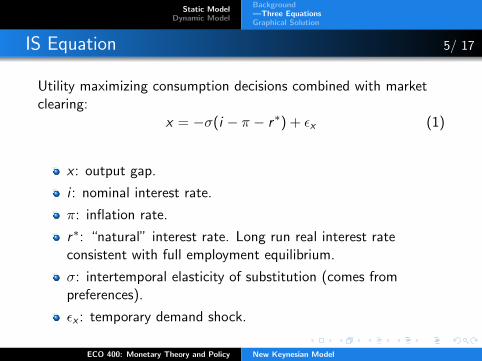
Utility maximizing consumption decisions combined with marketclearing:
x = −σ(i − π − r∗) + εx (1)
x : output gap.
i : nominal interest rate.
π: inflation rate.
r∗: “natural” interest rate. Long run real interest rateconsistent with full employment equilibrium.
σ: intertemporal elasticity of substitution (comes frompreferences).
εx : temporary demand shock.
ECO 400: Monetary Theory and Policy New Keynesian Model

Static ModelDynamic Model
Background—Three EquationsGraphical Solution
IS Equation 5/ 17
Utility maximizing consumption decisions combined with marketclearing:
x = −σ(i − π − r∗) + εx (1)
x : output gap.
i : nominal interest rate.
π: inflation rate.
r∗: “natural” interest rate. Long run real interest rateconsistent with full employment equilibrium.
σ: intertemporal elasticity of substitution (comes frompreferences).
εx : temporary demand shock.
ECO 400: Monetary Theory and Policy New Keynesian Model

Static ModelDynamic Model
Background—Three EquationsGraphical Solution
Phillips Curve 6/ 17
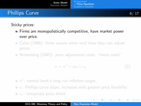
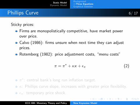
Sticky prices:
Firms are monopolistically competitive, have market powerover price.
Calvo (1986): firms unsure when next time they can adjustprices.
Rotemberg (1982): price adjustment costs, “menu costs”
π = π∗ + κx + επ (2)
π∗: central bank’s long run inflation target.
κ: Phillips curve slope, increases with greater price flexibility.
επ: temporary price shock.
ECO 400: Monetary Theory and Policy New Keynesian Model
Static ModelDynamic Model
Background—Three EquationsGraphical Solution
Phillips Curve 6/ 17
Sticky prices:
Firms are monopolistically competitive, have market powerover price.
Calvo (1986): firms unsure when next time they can adjustprices.
Rotemberg (1982): price adjustment costs, “menu costs”
π = π∗ + κx + επ (2)
π∗: central bank’s long run inflation target.
κ: Phillips curve slope, increases with greater price flexibility.
επ: temporary price shock.
ECO 400: Monetary Theory and Policy New Keynesian Model

Static ModelDynamic Model
Background—Three EquationsGraphical Solution
Taylor Rule 7/ 17
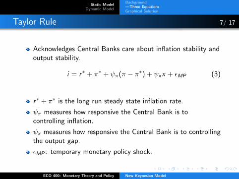
Acknowledges Central Banks care about inflation stability andoutput stability.
i = r∗ + π∗ + ψπ(π − π∗) + ψxx + εMP (3)
r∗ + π∗ is the long run steady state inflation rate.
ψπ measures how responsive the Central Bank is tocontrolling inflation.
ψx measures how responsive the Central Bank is to controllingthe output gap.
εMP : temporary monetary policy shock.
ECO 400: Monetary Theory and Policy New Keynesian Model

Static ModelDynamic Model
Background—Three EquationsGraphical Solution
Taylor Rule 7/ 17
Acknowledges Central Banks care about inflation stability andoutput stability.
i = r∗ + π∗ + ψπ(π − π∗) + ψxx + εMP (3)
r∗ + π∗ is the long run steady state inflation rate.
ψπ measures how responsive the Central Bank is tocontrolling inflation.
ψx measures how responsive the Central Bank is to controllingthe output gap.
εMP : temporary monetary policy shock.
ECO 400: Monetary Theory and Policy New Keynesian Model

Static ModelDynamic Model
Background—Three EquationsGraphical Solution
Aggregate Supply / Aggregate Demand 8/ 17
Substitute Taylor rule into IS curve to get Aggregate Demand:
x = −σ(ψπ − 1)
1 + σψx(π − π∗) + εD , (4)
where, εD ≡1
1 + σψx(−σεMP + εx)
Aggregate Supply curve ≡ Phillips curve:
π − π∗ = κx + επ
Downward sloping demand curve if and only if ψπ > 1.
Clarida et al (1999): In a dynamic model this is the conditionfor stability.
ECO 400: Monetary Theory and Policy New Keynesian Model

Static ModelDynamic Model
Background—Three EquationsGraphical Solution
New Keynesian Model 9/ 17
ECO 400: Monetary Theory and Policy New Keynesian Model

Static ModelDynamic Model
Background—Three EquationsGraphical Solution
Demand Shock 10/ 17
Economy is hit with a positive exogenous demand shock,εD is positive.
ECO 400: Monetary Theory and Policy New Keynesian Model

Static ModelDynamic Model
Background—Three EquationsGraphical Solution
Demand Shock 10/ 17
IS and AD curves shift to the right.Increase in output gap and inflation in equilibrium.
ECO 400: Monetary Theory and Policy New Keynesian Model

Static ModelDynamic Model
Background—Three EquationsGraphical Solution
Demand Shock 10/ 17
Increase in inflation shifts Taylor rule upward.Further increase in interest rates shifts AD left.
ECO 400: Monetary Theory and Policy New Keynesian Model

Static ModelDynamic Model
Background—Three EquationsGraphical Solution
Demand Shock 10/ 17
Size of Taylor rule and second AD shifts demand on size of Taylorrule coefficients.
ECO 400: Monetary Theory and Policy New Keynesian Model

Static ModelDynamic Model
Background—Three EquationsGraphical Solution
Cost Shock 11/ 17
Economy is hit with a positive exogenous cost shock.
ECO 400: Monetary Theory and Policy New Keynesian Model

Static ModelDynamic Model
Background—Three EquationsGraphical Solution
Cost Shock 11/ 17
Phillips Curve shifts left.
ECO 400: Monetary Theory and Policy New Keynesian Model

Static ModelDynamic Model
Background—Three EquationsGraphical Solution
Cost Shock 11/ 17
Increase in inflation shifts Taylor rule left.
ECO 400: Monetary Theory and Policy New Keynesian Model

Static ModelDynamic Model
Background—Three EquationsGraphical Solution
Cost Shock 11/ 17
Increase in inflation also causes a rightward shift in IS curve.
ECO 400: Monetary Theory and Policy New Keynesian Model

Static ModelDynamic Model
Three Equation ModelExpectationsDiscussion
Dynamic Model: IS Equation 12/ 17
Microfounded decisions depend on expectations of futurevariables.
xt = E ∗t xt+1 − σ(rt − E ∗
t πt+1 − r∗) + εx ,t (5)
E ∗t denotes time t expectation of what follows.
Et is more specific, denotes time t rational expectation ofwhat follows.
Decisions about consumption today depend on expectedfuture consumption (E ∗
t xt+1).
Decisions about consumption today depends on expected realinterest rate.
ECO 400: Monetary Theory and Policy New Keynesian Model

Static ModelDynamic Model
Three Equation ModelExpectationsDiscussion
Phillips Curve 13/ 17
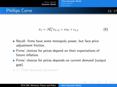
πt = βE ∗t πt+1 + κxt + επ,t (6)
Recall: firms have some monopoly power, but face priceadjustment friction.
Firms’ choices for prices depend on their expectations offuture inflation.
Firms’ choices for prices depends on current demand (outputgap).
β: Time discount parameter.
ECO 400: Monetary Theory and Policy New Keynesian Model

Static ModelDynamic Model
Three Equation ModelExpectationsDiscussion
Phillips Curve 13/ 17
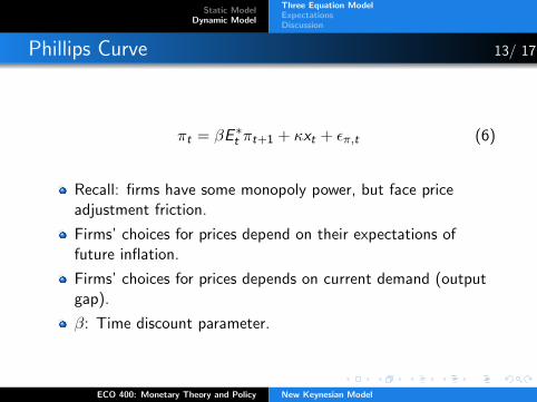
πt = βE ∗t πt+1 + κxt + επ,t (6)
Recall: firms have some monopoly power, but face priceadjustment friction.
Firms’ choices for prices depend on their expectations offuture inflation.
Firms’ choices for prices depends on current demand (outputgap).
β: Time discount parameter.
ECO 400: Monetary Theory and Policy New Keynesian Model

Static ModelDynamic Model
Three Equation ModelExpectationsDiscussion
Phillips Curve 13/ 17
πt = βE ∗t πt+1 + κxt + επ,t (6)
Recall: firms have some monopoly power, but face priceadjustment friction.
Firms’ choices for prices depend on their expectations offuture inflation.
Firms’ choices for prices depends on current demand (outputgap).
β: Time discount parameter.
ECO 400: Monetary Theory and Policy New Keynesian Model

Static ModelDynamic Model
Three Equation ModelExpectationsDiscussion
Taylor Rule 14/ 17
Handful of Taylor rules to consider.
Fed may only gradually adjust the federal funds rate.
Fed may target current realizations of x and π:
rt = ρrt−1 + (1− ρ) [ψπ(πt − π∗) + ψxxt ] (7)
ρ ∈ (0, 1) is the degree of adjustment. Smaller ρ means fasteradjustment.
Fed may target expectations of x and/or π:
rt = ρrt−1+(1−ρr ) [ψπ(E ∗t πt+1 − π∗) + ψxE
∗t xt+1]+εr ,t (8)
rt = ρrt−1 + (1− ρr ) [ψπ(E ∗t πt − π∗) + ψxE
∗t xt ] + εr ,t (9)
ECO 400: Monetary Theory and Policy New Keynesian Model

Static ModelDynamic Model
Three Equation ModelExpectationsDiscussion
Rational Expectations 15/ 17
People in the economy know the model.
They can identify quantities of shocks: εx ,t , επ,t , εr ,t .
They know the values of the parameters: κ, σ, β.
They have taken a couple years of calculus courses andgraduate macroeconomics courses and know how to solve themodel.
Set Etεx ,t = Etεπ,t = Etεr ,t = 0, use solution for expectations.
ECO 400: Monetary Theory and Policy New Keynesian Model

Static ModelDynamic Model
Three Equation ModelExpectationsDiscussion
Adaptive Expectations 16/ 17
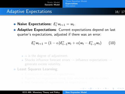
Naive Expectations: E ∗t wt+1 = wt .
Adaptive Expectations: Current expectations depend on lastquarter’s expectations, adjusted if there was an error:
E ∗t wt+1 = (1− α)E ∗
t−1wt + α(wt − E ∗t−1wt) (10)
α is the degree of adjustment.Shocks influence forecast errors → influence expectations →generate excess volatility.
Least Squares Learning:
Extension of adaptive expectations.Agents run regressions using data anyone is able to collect.Use forecasts of regressions as expectations.
ECO 400: Monetary Theory and Policy New Keynesian Model

Static ModelDynamic Model
Three Equation ModelExpectationsDiscussion
Adaptive Expectations 16/ 17
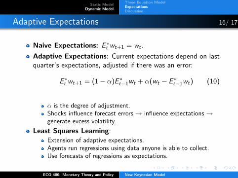
Naive Expectations: E ∗t wt+1 = wt .
Adaptive Expectations: Current expectations depend on lastquarter’s expectations, adjusted if there was an error:
E ∗t wt+1 = (1− α)E ∗
t−1wt + α(wt − E ∗t−1wt) (10)
α is the degree of adjustment.Shocks influence forecast errors → influence expectations →generate excess volatility.
Least Squares Learning:
Extension of adaptive expectations.Agents run regressions using data anyone is able to collect.Use forecasts of regressions as expectations.
ECO 400: Monetary Theory and Policy New Keynesian Model
Static ModelDynamic Model
Three Equation ModelExpectationsDiscussion
Adaptive Expectations 16/ 17
Naive Expectations: E ∗t wt+1 = wt .
Adaptive Expectations: Current expectations depend on lastquarter’s expectations, adjusted if there was an error:
E ∗t wt+1 = (1− α)E ∗
t−1wt + α(wt − E ∗t−1wt) (10)
α is the degree of adjustment.Shocks influence forecast errors → influence expectations →generate excess volatility.
Least Squares Learning:
Extension of adaptive expectations.Agents run regressions using data anyone is able to collect.Use forecasts of regressions as expectations.
ECO 400: Monetary Theory and Policy New Keynesian Model

Static ModelDynamic Model
Three Equation ModelExpectationsDiscussion
Benefits and Drawbacks 17/ 17
Benefits:
Can trace out predictions of variables across time.Can generate impulse response functions.Specific predictions about time, not general “long run” and“short run”.Possible to estimate this model using time series of outputgap, inflation, federal funds rate.Simple but robust specification allows for lots of extensions(expectation assumptions).
Drawbacks:
Difficult to draw. Need a set of graphs for each time t.Overly simple - only three variables, three equations, closedeconomy, no investment, no government.
ECO 400: Monetary Theory and Policy New Keynesian Model