New Decomposition Methods for Home Care Scheduling with ...

New Decomposition Methods for Home Care Scheduling with Predefined Visits Florian Grenouilleau Nadia Lahrichi Louis-Martin Rousseau March 2019

CIRRELT-2019-10

New Decomposition Methods for Home Care Scheduling with Predefined Visits

Florian Grenouilleau*, Nadia Lahrichi, Louis-Martin Rousseau

Interuniversity Research Centre on Enterprise Networks, Logistics and Transportation (CIRRELT) and Department of Mathematics and Industrial Engineering, Polytechnique Montréal

Abstract. The continuous aging of the population and the desire of the elderly to stay in their own

homes as long as possible has led to a considerable increase in the demand for home visits.

Home care agencies try to serve more patients while maintaining a high level of service. They

must regularly decide which patients they can accept and how the patients will be scheduled (care

provider, visit days, visit times). In this paper we aim to maximize the number of new patients

accepted while ensuring a single provider-to-patient assignment and a synchronization of the visit

times for every patient. To solve this problem, we propose an extension to an existing logic-based

Benders decomposition. Moreover, we present a new pattern-based logic-based Benders

decomposition and a matheuristic using a large neighborhood search. The experiments

demonstrate the efficiency of the proposed approaches and show that the matheuristic can solve

all the benchmark instances in less than 20 seconds.

Keywords: Home care, scheduling, LBBD, matheuristic, LNS.

Acknowledgements. We thank Aliza Heching, John Hooker, and Ryo Kimura for providing

access to the benchmark instances. This work has been supported by the Canadian Research

Chair in HealthCare Analytic and Logistic and the Natural Sciences and Engineering Research

Council of Canada.

Results and views expressed in this publication are the sole responsibility of the authors and do not necessarily reflect those of CIRRELT.

Les résultats et opinions contenus dans cette publication ne reflètent pas nécessairement la position du CIRRELT et n'engagent pas sa responsabilité. _____________________________ * Corresponding author: [email protected] Dépôt légal – Bibliothèque et Archives nationales du Québec

Bibliothèque et Archives Canada, 2019

© Grenouilleau, Lahrichi, Rousseau and CIRRELT, 2019

1. Introduction

Due to population aging and the government’s plan to decentralize care,

the demand for home care services has significantly increased during the last

decade. These services allow the patients to stay in their own homes for as

long as possible. From the government’s point of view, home care services

reduce the patient flow in hospitals and reduce the cost of care. Home care

agencies continuously try to better manage their resources in order to serve

more patients while maintaining a high level of service.

During the past ten years, many researchers have considered the rout-

ing and scheduling aspects of the problem (see Bertels & Fahle (2006),

Nickel et al. (2012), Hiermann et al. (2015) and Grenouilleau et al. (2017)).

The goal is to visit sets of patients while reducing costs (travel time, over-

time) and/or maximizing soft constraints (patients’ preferences, continuity

of care). Recently, there have been two comprehensive surveys of the home

health care routing and scheduling problem (Cisse et al., 2017; Fikar &

Hirsch, 2017).

Home care agencies also wish to accept as many new patients as possible.

This aspect of the problem has already been studied in the literature such

as in (De Angelis, 1998) and (Koeleman et al., 2012). Heching et al. (2019)

present a problem in which the goal is to schedule as many new patients as

possible while taking into account those already present in the system (their

visits cannot be rescheduled). In this challenging problem, only one care

provider can be assigned to each patient, and the visit times must be the

same over the entire horizon (one week). Moreover, restrictions on the travel

times and the maximum working time of each provider must be respected.

We refer to this as home care scheduling with predefined visits (HCS-PV).

2


CIRRELT-2019-10

Heching et al. (2019) proposed a logic-based Benders decomposition (LBBD)

(Hooker & Ottosson, 2003).

The LBBD method has scalability issues. It is unable to solve some

of the benchmark instances in a reasonable time (1 hour), and the time

increases significantly with the difficulty of the instance. In this paper, we

present three approaches based on decomposition methods that are able to

solve all the benchmark instances while reducing the overall computational

time.

Our contributions are as follows. We firstly propose a new algorithm

for the subproblem of the LBBD formulation presented in Heching et al.

(2019). It decomposes the subproblem to make it easier to solve. Secondly,

we present a new LBBD formulation with additional variables. The new

variables correspond to visit patterns for new patients; they combine the

assigned provider, the visit days, and the visit times in a single variable so

that most of the constraints can be handled in the master problem. Finally,

we propose a new matheuristic method based on a Dantzig–Wolfe formu-

lation (DWF) and a large neighborhood search (LNS). This matheuristic

iteratively solves the problem using LNS and then solves the DWF using

the providers’ schedules found during the LNS iterations. Our computa-

tional experiments show that the matheuristic finds all the solutions of the

benchmark instances in less than 20 seconds.

The remainder of this paper is as follows. Section 2 defines the problem.

Section 3 presents the mathematical formulations, and Section 4 describes

our matheuristic. Section 5 presents the computational results and Section

6 provides concluding remarks.

3


CIRRELT-2019-10

2. Problem definition

HCS-PV considers a patient set P and maximizes the number of sched-

uled patients given a set of available providers A. For each scheduled pa-

tient, we must determine the assigned provider, the visit days, and the visit

time. These decisions must take into account the existing patients (called

the “fixed” patients); the scheduled visits for the fixed patients cannot be

modified. This constraint arises from the requirement for continuity of care.

In the home care context, continuity of care involves always sending the

same provider at the same time to the same patient, to build a relation-

ship between them and to improve the patient’s experience. Figure 1 gives

an example of a provider’s schedule and a possible slot for a new patient

requiring two visits per week.

Figure 1: Possible assignment for a new patient requiring two visits per week.

Various assignment and routing constraints must be taken into account.

Each patient is assigned to a single provider, and the visit times must be

the same throughout the week (visit synchronization). There are also re-

strictions on the travel time, the available time windows for the patients

4


CIRRELT-2019-10

and providers, and the maximum weekly working time for the providers.

Formally, each patient p has a required number of visits vp ∈ [1, 5], a visit

duration durp, a location lp and a time window [rp, dp] in which he/she

must be visited. Moreover, some patients have special requirements, e.g.,

they may need a specified duration between visits. For this constraint we

define the set Kp of possible day groups for patient p. Finally, each provider

a has a location la with a service time equal to zero, a working time window

[ra, da], and a maximum working time Wa over the week. The working time

only comprises the time between the start of the first patient and the end

of the last patient for each work day.

3. Mathematical formulations

In this section, we present three mathematical formulations. Firstly,

we present the LBBD formulation (Heching et al., 2019) and propose an

alternative subproblem. Secondly, we present another LBBD formulation

based on visit patterns. Finally, we introduce a classical DWF.

3.1. Assignment-based LBBD

This first formulation (Heching et al., 2019) uses an LBBD (Hooker &

Ottosson, 2003), which derives from the classical Benders decomposition

(Benders, 1962). The classical Benders method decomposes the problem

into two parts (master problem and subproblem). It iteratively solves the

master problem and checks the feasibility and optimality of the solution in

the subproblem. If necessary, the subproblem generates feasibility and/or

optimality cuts, and these cuts are added to the master problem. The

process stops when the generated solution is optimal or the problem is proved

5


CIRRELT-2019-10

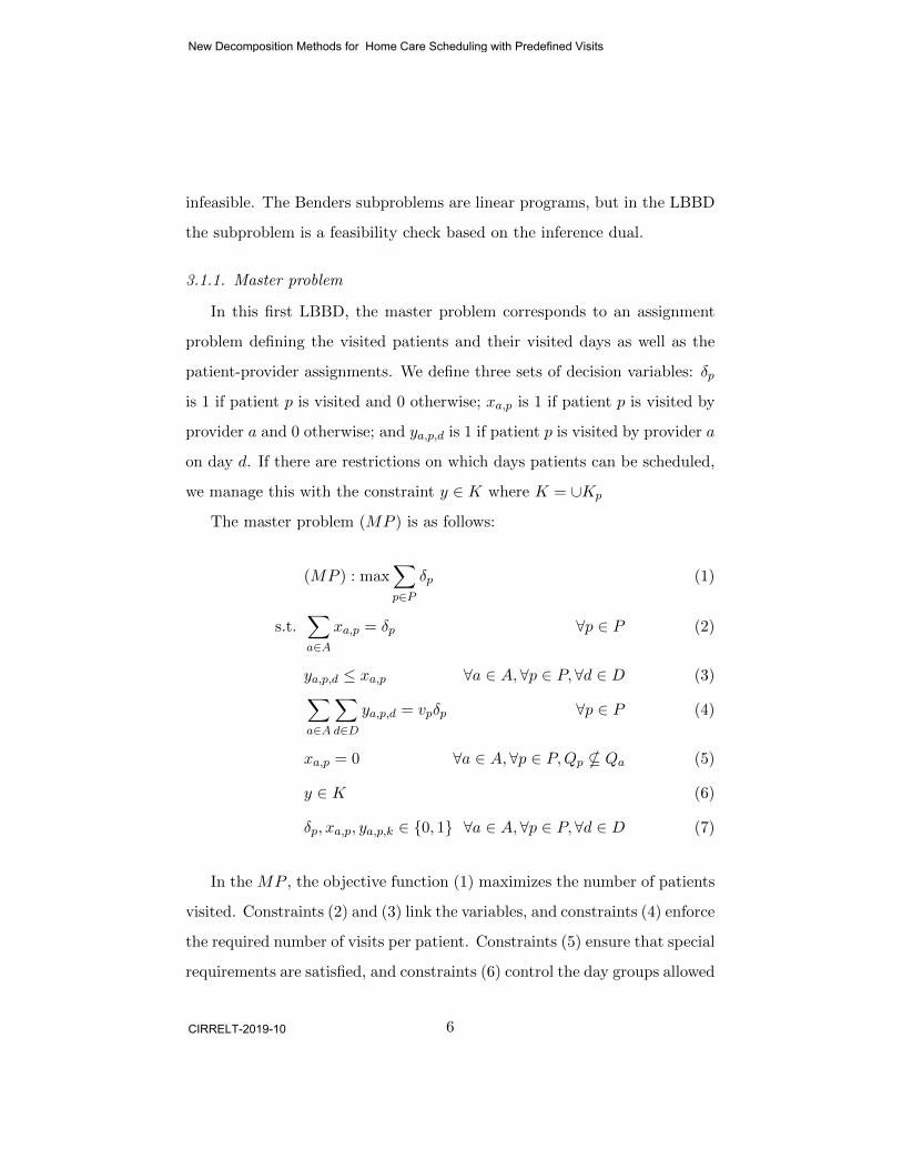
infeasible. The Benders subproblems are linear programs, but in the LBBD

the subproblem is a feasibility check based on the inference dual.

3.1.1. Master problem

In this first LBBD, the master problem corresponds to an assignment

problem defining the visited patients and their visited days as well as the

patient-provider assignments. We define three sets of decision variables: δp

is 1 if patient p is visited and 0 otherwise; xa,p is 1 if patient p is visited by

provider a and 0 otherwise; and ya,p,d is 1 if patient p is visited by provider a

on day d. If there are restrictions on which days patients can be scheduled,

we manage this with the constraint y ∈ K where K = ∪Kp

The master problem (MP ) is as follows:

(MP ) : max∑p∈P

δp (1)

s.t.∑a∈A

xa,p = δp ∀p ∈ P (2)

ya,p,d ≤ xa,p ∀a ∈ A,∀p ∈ P,∀d ∈ D (3)∑a∈A

∑d∈D

ya,p,d = vpδp ∀p ∈ P (4)

xa,p = 0 ∀a ∈ A,∀p ∈ P,Qp * Qa (5)

y ∈ K (6)

δp, xa,p, ya,p,k ∈ 0, 1 ∀a ∈ A,∀p ∈ P,∀d ∈ D (7)

In the MP , the objective function (1) maximizes the number of patients

visited. Constraints (2) and (3) link the variables, and constraints (4) enforce

the required number of visits per patient. Constraints (5) ensure that special

requirements are satisfied, and constraints (6) control the day groups allowed

6


CIRRELT-2019-10

for each patient. Finally, constraints (7) are the binary restrictions.

3.1.2. Subproblem

The subproblem determines if the assignment found by MP is feasible, if

not, no-good cuts (on the ya,p,d variables) are added to the master problem.

We define a subproblem SP for each provider. Each SP corresponds to

a multiple-day traveling salesman problem with time windows, and it is

solved using constraint programming. For each SP, we define P(SP ) the set

of assigned patients and P(SP ),d the set of patients assigned per day d. In

addition, we define sequencing variables πd,v that correspond to the patient

p visited in the vth position on day d, with p ∈ P(SP ),d. These variables

also take into account the fact that each route must start and end at the

provider’s location la. We also define the variables sp corresponding to the

visit time for patient p. Finally, we set the value VP equal to |P(SP ),d|. We

define a subproblem for each provider as follows:

(SP ) : max 0 (8)

s.t. all differentπd,v|v = 1, .., VP + 2 ∀d ∈ D (9)

πd,1 = la, πd,VP +2 = la ∀d ∈ D (10)

rp ≤ sp ≤ dp − durp ∀p ∈ P(SP ) (11)

sπd,v + durπd,v + tπd,v ,πd,v+1≤ sπd,v+1

∀d ∈ D, v = 1, .., VP + 1 (12)∑d∈D

(sπd,VP+1+ durπd,VP+1

− sπd,2) ≤Wa (13)

πd,v ∈ P(SP ),d ∪ la ∪ la′ ∀d ∈ D, v = 1, .., VP + 2 (14)

In this formulation, the objective function (8) is 0 because we simply

7


CIRRELT-2019-10

want to verify if a solution exists. Constraints (9) are the patient sequenc-

ing constraints. Constraints (10) ensure that the provider starts and ends

each day at his/her home, and constraints (11) enforce the patients’ time

windows. The travel time constraints are taken into account by constraints

(12) and the maximum working time by constraints (13). The working time

constraint measures the time between the start of the first patient and the

end of the last one. Finally, the variables’ domains are defined by constraints

(14).

3.1.3. Alternative subproblem approach

The subproblem must consider all the routing constraints (travel time,

visit synchronization, overtime, time windows) and this could lead to an

excessive computational time. We therefore present an alternative approach.

We first solve the problem for each day independently, without taking into

account the provider’s maximum weekly working time. If a feasible route is

found for each day, we solve the full subproblem.

First, we introduce the constraint programming formulation of the daily

problem in which the index d is removed. The daily subproblem (SPd) is:

(SPd) : max 0 (15)

s.t. all differentπv|v = 1, .., VP + 2 (16)

π1 = la, πVP +2 = la (17)

rp ≤ sp ≤ dp − durp ∀p ∈ P(SP ),d (18)

sπv + durπv + tπv ,πv+1 ≤ sπv+1 v = 1, .., VP + 1 (19)

πv ∈ P(SP ),d ∪ la ∪ la′ v = 1, .., VP + 2 (20)

8


CIRRELT-2019-10

Algorithm 1 gives the two-stage solution method.

Algorithm 1: Alternative subproblem

1 for each day d of the horizon do

2 if (SPd) is not feasible then

3 Generate a feasibility cut and stop the search;

4 end if

5 end for

6 if Solve (SP ) is not feasible then

7 Generate a feasibility cut and stop the search;

8 end if

3.2. Pattern-based LBBD

We must determine for each patient the assigned provider, the set of

visit days, and the visit time. In the second formulation, we combine these

decisions into a new variable.

We introduce the concept of a visit pattern ω, with four elements: pa-

tient pω, assigned provider aω, set of visit days Dω, and visit time sω. The

problem involves assigning a pattern ω ∈ Ωp to each patient, where Ωp is

a set containing all the visit patterns for patient p, with ∪p∈PΩp = Ω. We

can compute in advance the set of feasible patterns for each patient, thus

generating the set Ω containing all the feasible patterns. Algorithm 2 gen-

erates the patterns.

9


CIRRELT-2019-10

Algorithm 2: Pattern Generation

1 Ω = ∅; // List of the possible patterns ;

2 for each patient p do

3 for each provider a do

4 for time index t ∈ [rp, lp] ∩ [ea, la] do

5 for each combination C of(

5vp

)days do

6 if the pattern made of provider a, visit time t, and visit

days C is feasible for patient p then

7 Add the pattern to Ω;

8 end if

9 end for

10 end for

11 end for

12 end for

3.2.1. Master problem

We now present a new LBBD formulation based on Ω. Let the variable

zp be 1 if patient p is visited and 0 otherwise, and let xω be 1 if visit pattern

ω is selected. Finally, ttω,ω′ corresponds to the travel time between the

patient locations associated with patterns ω and ω′.

In the pattern-based formulation (PBF), the master problem is a set cov-

ering problem defined by (21)–(25). The objective function (21) maximizes

the number of patients visited. Constraints (22) link the decision variables,

and constraints (23) enforce the travel time between patients. Constraints

(24)–(25) are the binary restrictions.

10


CIRRELT-2019-10

(PBF ) : max∑p∈P

zp (21)

s.t. zp =∑ωp∈Ωp

xωp ∀p ∈ P (22)

xω + xω′ ≤ 1 ∀(ω, ω′) ∈ Ω, Dω ∩Dω′ 6= ∅, sω + ttω,ω′ > sω′ (23)

zp ∈ 0, 1 ∀p ∈ P (24)

xω ∈ 0, 1 ∀ω ∈ Ω (25)

3.2.2. Subproblem

The new master problem includes all the constraints (single provider-

to-patient assignment, synchronized visits, required number of visits, travel

time, patient requirements) except the restrictions on the providers’ working

time, which are enforced in the subproblems. Algorithm 3 presents a simple

polynomial algorithm for the solution of the subproblems.

Algorithm 3: Subproblem solution (for provider a)

1 sum work time = 0 ;

2 for each day d of the horizon do

3 Retrieve the list Ld of assigned patterns containing this day;

4 Sort ld by increasing order of visit times and build the route rd;

5 sum work time += rd’s work time;

6 end for

7 if sum work time > Wa then

8 Create a no-good cut on the assigned patterns;

9 end if

11


CIRRELT-2019-10

3.3. Dantzig-Wolfe decomposition

In Section 3.2, each patient has an associated visit pattern, and so each

provider has a list of assigned visit patterns corresponding to his/her weekly

schedule. In this third formulation, we base our model on the providers’

assignments. A feasible provider assignment corresponds to a subset of visit

patterns that satisfies the travel and work-time constraints.

Let Λ be the set of feasible provider assignments, with Λa the set of

feasible assignments for provider a. Let nλ be the number of patients visited

by assignment λ. We set vλ,p to 1 if patient p is visited by assignment λ

and 0 otherwise. Finally, we define the decision variable xλ, which is 1 if

provider assignment λ is selected and 0 otherwise.

The assignment set partitioning formulation (ASP) is a Dantzig–Wolfe

decomposition and is as follows:

(ASP ) : max∑λ∈Λ

nλxλ (26)

s.t.∑λ∈Λa

xλ ≤ 1 ∀a ∈ A (27)

∑λ∈Λ

vλ,pxλ ≤ 1 ∀p ∈ P (28)

xλ ∈ 0, 1 ∀λ ∈ Λ (29)

The objective function (26) maximizes the number of patients scheduled.

Constraints (27) ensure that there is at most one assignment per provider,

and constraints (28) ensure that there is at most one assignment per patient.

Finally, constraints (29) are the binary restrictions.

12


CIRRELT-2019-10

4. Visit pattern matheuristic

In this section, we present a visit pattern matheuristic based on the

formulation in Section 3.3 and an LNS. The LNS (Shaw, 1998) is a meta-

heuristic using the ruin-and-recreate principle (Schrimpf et al., 2000). This

iterative method destroys part of the solution and then repairs it to improve

its quality. The current and best solutions are then updated if necessary.

According to the literature, matheuristics provide a good balance be-

tween the solution quality of an exact method and the short computational

time of metaheuristics. We have developed a visit pattern matheuristic

(VPM) that uses an LNS to generate feasible provider assignments and then

solves (26)–(29) using these assignments. Such a method has already been

used in the home care context (Grenouilleau et al., 2017). In this paper, the

set partitioning was on the daily routes while here we capture the provider’s

schedule for the entire horizon. We study the ability of this matheuristic to

quickly generate interesting provider assignments, making it possible to find

good solutions rapidly.

4.1. Overview of visit pattern metaheuristic

Algorithm 4 gives an overview of the VPM. We first create an initial

solution and then iteratively remove part of the solution using a removal

operator and rebuild it using a repair operator. We then analyze the tem-

porary solution (St) to see if it improves the best found solution (S∗) or if

the acceptance rule (simulated annealing in our context) accepts it as the

current solution (Si). We solve the set partitioning problem based on Λ

every 2000 iterations and update the current and best solutions if necessary.

13


CIRRELT-2019-10

The implementation details are given in Section 4.2

Algorithm 4: VPM

1 Create the initial solution Sc;

2 Set the best found solution S∗ to Sc;

3 Create the empty set of provider assignments Λ;

4 while termination criterion not met do

5 St ← Sc;

6 Apply removal operator to St;

7 Apply repair operator to St;

8 Add the assignments to Λ;

9 if St is accepted then

10 Sc ← St;

11 end if

12 if St is better than S∗ then

13 S∗ ← St;

14 end if

15 if total iteration % 2000 = 0 then

16 Ssp ← Solve ASP based on Λ;

17 if Ssp better than S∗ then

18 S∗ ← Ssp;

19 Sc ← Ssp;

20 end if

21 end if

22 end while

4.2. Implementation details

We now present the implementation details of our LNS algorithm.

14


CIRRELT-2019-10

4.2.1. Initial solution

Algorithm 5 builds the initial solution using a greedy approach.

Algorithm 5: Initial Solution

1 Create P ′, a copy of the patient set P ;

2 Create the solution Si with fixed visit patterns per provider;

3 while P ′ is not empty do

4 Randomly select patient pt from P ′;

5 Remove pt from P ′;

6 Find all the feasible insertions Ipt for pt’s visit patterns;

7 if Ipt is not empty then

8 Apply to Si the insertion giving the smallest increase in the

travel time;

9 end if

10 return solution Si;

11 end while

4.2.2. Destroy and repair operators

We have adapted the classical removal and destroy operators from Shaw

(1998) and Ropke & Pisinger (2006). These operators work on the feasible

visit patterns described in Section 3.2. We list the operators here with

brief descriptions. The removal operator (Ropke & Pisinger, 2006) removes

q patients per iteration, and we set q to 30% of the number of scheduled

patients. We define Cp,n to be the increase in the travel time arising from

the insertion of patient p’s nth best option.

Random removal. This operator randomly selects q scheduled patients and

removes their visit patterns from the solution.

15


CIRRELT-2019-10

Worst removal. This operator computes, for each patient, the improvement

in the travel time if the patient’s visit pattern is removed. It then removes

the q patients with the highest values.

Related removal. This operator randomly selects a patient and removes

his/her visit pattern. Then it removes the q − 1 most closely related pa-

tients. In our implementation, the relation between two patients is based on

the percentage of shared time windows and the required number of visits:

R(p, p′) =[rp,dp]∩[rp′ ,dp′ ]

dp−rp +min(1,vp′vp

).

Random repair. This operator randomly selects an unscheduled patient p,

computes the possible insertions of p’s visit patterns, and applies the inser-

tion with the lowest cost. This operation is repeated until all the unsched-

uled patients have been tested.

Greedy repair. This operator iteratively computes the possible insertions for

the unscheduled patients and applies the insertion associated with argminp∈PCp,1.

This operation is repeated until there are no more possible insertions.

Regret repair. This operator iteratively computes the possible insertions of

the unscheduled patients and applies the best insertion for the patient with

the highest regret value. Patient p’s regret value is Cp,2 − Cp,1.

4.2.3. Acceptance rule

The acceptance rule determines if the created solution can be accepted

as the new current solution. It is based on simulated annealing as described

in Ropke & Pisinger (2006). We set our initial temperature to 1.05 ∗ f(Si)

and the decreasing temperature c to 0.99975.

16


CIRRELT-2019-10

4.2.4. Termination criteria

The termination of our LNS algorithm is based on two termination cri-

teria: we stop after 20,000 iterations or 20 seconds of computation.

5. Computational results

In this section, we present experiments that analyze the efficiency of our

alternative subproblem, the pattern-based formulation, and the matheuris-

tic. We use the instances of Heching et al. (2019), and we have re-implemented

their method, including their overtime and time-window relaxations. We

refer to their formulation as Heching. Heching et al. (2019) provided 57

instances, each with 60 patients, those instances are split into three sets:

• Classical : Instances provided by their industrial partner;

• Narrow : Based on the Classical instances, with narrow patient time

windows;

• Fewer : Based on the Classical instances, with fewer visits per patient.

We implemented the methods in C++ and performed the tests on a

2.7 GHz Intel Core i5 Macbook, with 16 Gb RAM and only one core. We

solve the master problems (1)–(7) and (21)–(25) using Cplex 12.7.1 and the

subproblems (8)–(14) and (15)–(20) using CP Optimizer. Finally, for the

LBBDs, the maximum computational time is set to 3600 s per instance.

5.1. Efficiency of the LBBD formulations

We now analyze the impact of the alternative subproblem (3.1) and the

pattern-based formulation (PBF). The results are given in Table 1. The

first three columns present the instance name, the number of new patients

17


CIRRELT-2019-10

(a value of 6 indicates 6 new patients and 54 fixed patients), and the optimal

solution. The CPU column gives the computational time in seconds. Fi-

nally, for PBF, Nb Pattern gives the number of feasible patterns computed

and TL is the time limit (3600 s).

We observe that using the alternative subproblem dramatically reduces

the computational time (-36.14%) and outperforms Heching for 51 of 55

solved instances. It performs especially well for the small and Fewer in-

stances. In addition, according to Figure 2, Heching’ subproblem has a

failure rate (Heching - Inf SP) of 80.65% in average while the alternative

subproblem only calls the whole subproblem (Alternative - Call SP) 30.70%

of the time and the subproblem is infeasible (Alternative - Inf SP) only for

28.74% of those calls.

For the Classical and Narrow instances, the PBF dramatically outper-

forms the model proposed in Heching et al. (2019) even with the alternative

subproblem. The PBF solves all the Classical instances in less than 9 s and

all the Narrow instances in less than 2 s. However, for the Fewer instances,

starting from 22 new patients, PBF does not outperform Heching. This is

because of the increase in the generated patterns and therefore the size of

the set partitioning problem. Nevertheless, PBF solves all the benchmark

instances.

18


CIRRELT-2019-10

Heching Alt. Subp. PBFInstance New Patients Optimal Value CPU (s) CPU (s) % Gap CPU (s) % Gap Nb Pattern

Classic 8 8 60 1.05 0.59 -43.81% 0.01 -99.05% 277Classic 9 9 59 0.96 0.71 -26.04% 0.01 -98.96% 276Classic 10 10 59 1.34 0.83 -38.06% 0.02 -98.51% 358Classic 11 11 59 1.26 1.15 -8.73% 0.02 -98.41% 405Classic 12 12 59 1.53 1.42 -7.19% 0.02 -98.69% 441Classic 13 13 59 2.12 0.85 -59.91% 0.05 -97.64% 551Classic 14 14 58 8.85 5.75 -35.03% 0.11 -98.76% 690Classic 15 15 58 8.79 6.30 -28.33% 0.11 -98.75% 724Classic 16 16 58 14.27 6.06 -57.53% 0.16 -98.88% 865Classic 17 17 59 12.81 11.54 -9.91% 0.45 -96.49% 1171Classic 18 18 58 22.14 14.11 -36.27% 0.53 -97.61% 1214Classic 19 19 58 31.93 30.79 -3.57% 0.87 -97.28% 1275Classic 20 20 57 97.78 47.67 -51.25% 0.7 -99.28% 1325Classic 21 21 58 210.34 86.18 -59.03% 1.2 -99.43% 1403Classic 22 22 58 185.70 96.46 -48.06% 0.91 -99.51% 1535Classic 23 23 58 1048.01 1557.68 48.63% 5.31 -99.49% 1913Classic 24 24 58 TL TL / 5.32 / 2032Classic 25 25 59 646.88 676.69 4.61% 3.3 -99.49% 2309Classic 26 26 59 2088.62 532.45 -74.51% 8.44 -99.60% 2543

Fewer 12 12 58 1.25 1.03 -17.60% 0.07 -94.40% 998Fewer 13 13 58 1.23 1.11 -9.76% 0.09 -92.68% 1158Fewer 14 14 58 2.15 1.35 -37.21% 0.12 -94.42% 1230Fewer 15 15 58 1.82 1.15 -36.81% 0.22 -87.91% 1584Fewer 16 16 58 2.20 1.58 -28.18% 0.3 -86.36% 1671Fewer 17 17 58 2.92 2.43 -16.78% 0.56 -80.82% 1989Fewer 18 18 58 3.87 2.08 -46.25% 0.68 -82.43% 2109Fewer 19 19 58 4.04 3.35 -17.08% 1.54 -61.88% 2484Fewer 20 20 59 4.78 2.11 -55.86% 2.02 -57.74% 2645Fewer 21 21 59 4.63 2.39 -48.38% 2.12 -54.21% 2954Fewer 22 22 59 4.85 2.28 -52.99% 2.53 -47.84% 3459Fewer 23 23 60 11.05 1.75 -84.16% 5.98 -45.88% 3693Fewer 24 24 60 4.78 2.55 -46.65% 4.12 -13.81% 3991Fewer 25 25 60 19.16 3.25 -83.04% 5.61 -70.72% 4536Fewer 26 26 60 5.09 1.59 -68.76% 5.61 10.22% 4875Fewer 27 27 60 21.70 4.27 -80.32% 29.74 37.05% 4950Fewer 28 28 60 49.97 13.64 -72.70% 125.98 152.11% 5108Fewer 29 29 59 78.30 21.17 -72.96% 83.68 6.87% 5196Fewer 30 30 59 398.6 221.64 -44.40% 3530.71 785.78% 5318

Narrow 8 8 60 0.95 0.67 -29.47% 0.01 -98.95% 243Narrow 9 9 59 1.33 0.88 -33.83% 0.01 -99.25% 242Narrow 10 10 59 1.67 0.75 -55.09% 0.01 -99.40% 296Narrow 11 11 59 1.29 0.79 -38.76% 0.01 -99.22% 308Narrow 12 12 59 0.97 1.03 6.19% 0.01 -98.97% 348Narrow 13 13 59 2.16 0.98 -54.63% 0.02 -99.07% 394Narrow 14 14 59 4.51 4.25 -5.76% 0.04 -99.11% 543Narrow 15 15 59 4.08 2.20 -46.08% 0.04 -99.02% 568Narrow 16 16 59 6.80 3.80 -44.12% 0.08 -98.82% 692Narrow 17 17 59 7.38 4.50 -39.02% 0.14 -98.10% 823Narrow 18 18 58 14.90 7.58 -49.13% 0.24 -98.39% 842Narrow 19 19 58 17.81 11.41 -35.93% 0.25 -98.60% 846Narrow 20 20 57 23.46 25.05 6.78% 0.49 -97.91% 860Narrow 21 21 57 34.24 25.47 -25.61% 0.54 -98.42% 878Narrow 22 22 57 73.74 68.79 -6.71% 0.5 -99.32% 948Narrow 23 23 58 190.47 129.74 -31.88% 1.23 -99.35% 1212Narrow 24 24 58 674.33 401.60 -40.44% 1.13 -99.83% 1317Narrow 25 25 58 TL TL / 1.38 / 1452Narrow 26 26 59 1303.29 1169.51 -10.26% 1.89 -99.85% 1594

Average -36.14% -64.30%

Table 1: Results for the alternative subproblem and visit pattern formulation

19


CIRRELT-2019-10

0 10 20 30 40 50 60

0

20

40

60

80

Instance

(%)

Heching - Inf SPAlternative - Call SPAlternative - Inf SP

Figure 2: Comparison of the failure rates during the full subproblems resolutions

5.2. Efficiency of the matheuristic

In this section, we test the visit pattern matheuristic (VPM) proposed

in Section 4. To do this, we solve the instances with the classical LNS

(i.e., without set partitioning) and with the VPM. The results are given in

Table 2. The columns Best and CPU Best correspond to the best found

solution and the time (in seconds) at which this solution was found. The

LNS solves 37 of the 57 instances in less than 20 s or 20,000 iterations. With

the same termination criteria, the VPM solves all the instances. For most

of the instances (51), the VPM finds the best solution in the first 10 s.

20


CIRRELT-2019-10

LNS VPMInstance New Patients Optimal Value Best Value CPU (s) CPU Best (s) Best Value CPU (s) CPU Best (s)

Classic 8 8 60 60 8.3 0.06 60 8.44 0.06Classic 9 9 59 59 8.32 0.16 59 8.44 0.16Classic 10 10 59 59 9.18 0.01 59 9.59 0.01Classic 11 11 59 59 11.85 0.11 59 12.1 0.11Classic 12 12 59 59 13.41 0.01 59 13.99 0.01Classic 13 13 59 59 16.21 0.03 59 14.92 0.03Classic 14 14 58 58 19.03 0.05 58 18.76 0.05Classic 15 15 58 58 18.51 0.03 58 18.92 0.03Classic 16 16 58 58 20 0.06 58 20 0.06Classic 17 17 59 59 20 17.03 59 20 4.16Classic 18 18 58 58 20 0.70 58 20 0.75Classic 19 19 58 58 20 3.12 58 20 3.17Classic 20 20 57 57 20 0.02 57 20 0.03Classic 21 21 58 57 20 5.53 58 20 10.49Classic 22 22 58 57 20 4.01 58 20 5.58Classic 23 23 58 57 20 1.12 58 20 6.88Classic 24 24 58 58 20 3.50 58 20 3.52Classic 25 25 59 58 20 8.35 59 20 16.18Classic 26 26 59 57 20 0.68 59 20 9.14

Fewer 12 12 58 58 20 0.16 58 20 0.16Fewer 13 13 58 58 20 0.04 58 20 0.04Fewer 14 14 58 58 20 0.02 58 20 0.01Fewer 15 15 58 58 20 1.01 58 20 1.03Fewer 16 16 58 58 20 0.09 58 20 0.09Fewer 17 17 58 58 20 0.09 58 20 0.10Fewer 18 18 58 58 20 0.15 58 20 0.15Fewer 19 19 58 58 20 1.04 58 20 1.04Fewer 20 20 59 58 20 0.25 59 20 6.29Fewer 21 21 59 59 20 1.69 59 20 1.96Fewer 22 22 59 59 20 5.26 59 20 4.83Fewer 23 23 60 59 20 0.16 60 20 8.79Fewer 24 24 60 60 20 0.84 60 20 0.80Fewer 25 25 60 60 20 16.66 60 20 9.61Fewer 26 26 60 60 20 12.62 60 20 10.41Fewer 27 27 60 59 20 0.29 60 20 11.19Fewer 28 28 60 59 20 3.84 60 20 12.2Fewer 29 29 59 59 20 9.99 59 20 9.45Fewer 30 30 59 58 20 7.55 59 20 13.93

Narrow 8 8 60 60 8.22 0.03 60 7.09 0.03Narrow 9 9 59 59 8.23 0.25 59 8.00 0.24Narrow 10 10 59 59 9.79 0.18 59 9.86 0.18Narrow 11 11 59 59 9.97 0.02 59 10.98 0.22Narrow 12 12 59 59 11.67 0.79 59 11.39 0.78Narrow 13 13 59 59 12.57 0.11 59 12.51 0.11Narrow 14 14 59 58 14.94 0.01 59 14.86 1.73Narrow 15 15 59 58 15.65 0.97 59 16.17 1.81Narrow 16 16 59 58 20 0.18 59 20 2.28Narrow 17 17 59 58 20 0.68 59 20 2.73Narrow 18 18 58 58 20 10.59 58 20 2.98Narrow 19 19 58 57 20 1.68 58 20 3.30Narrow 20 20 57 56 20 0.62 57 20 3.47Narrow 21 21 57 56 20 0.74 57 20 3.49Narrow 22 22 57 57 20 16.93 57 20 3.67Narrow 23 23 58 57 20 11.72 58 20 9.35Narrow 24 24 58 57 20 11.86 58 20 10.46Narrow 25 25 58 58 20 8.39 58 20 5.48Narrow 26 26 59 57 20 1.81 59 20 13.46

Average 17.82 3.05 17.84 3.83

Table 2: Results for the matheuristic

21


CIRRELT-2019-10

6. Conclusions

The HHC-PV is a complex problem that home care agencies have to solve

every day. The goal is to assign and schedule a set of new patients given a

set of providers while taking into account the patients already present in the

system. Each patient has a required number of visits and can be assigned to

only one provider. The visit times must be the same for the entire horizon,

and each provider has a maximum working time.

To solve this problem, we have extended the work of (Heching et al.,

2019). First, we proposed an alternative two-stage subproblem. Then, we

presented a new LBBD based on visit patterns that includes more con-

straints in the master problem. Finally, we introduced a Dantzif-Wolfe for-

mulation and developed a matheuristic based on LNS.

Our computational experiments show that our alternative subproblem

reduces the average computational time by 34%, while the new pattern-

based formulation solves all the benchmark instances, usually in less than

10 s. Finally, our matheuristic solves all the instances in less than 20 s.

In future research, we plan to take into account more practical con-

straints and to analyze how our formulations perform in such contexts.

Acknowledgment

We thank Aliza Heching, John Hooker, and Ryo Kimura for providing

access to the benchmark instances. This work has been supported by the

Canadian Research Chair in HealthCare Analytic and Logistic and the Nat-

ural Sciences and Engineering Research Council of Canada.

22


CIRRELT-2019-10

References

Benders, J. F. (1962). Partitioning procedures for solving mixed-variables

programming problems. Numerische Mathematik , 4 , 238–252.

Bertels, S., & Fahle, T. (2006). A hybrid setup for a hybrid scenario: combin-

ing heuristics for the home health care problem. Computers & Operations

Research, 33 , 2866–2890.

Cisse, M., Yalcındag, S., Kergosien, Y., Sahin, E., Lente, C., & Matta, A.

(2017). OR problems related to home health care: A review of relevant

routing and scheduling problems. Operations Research for Health Care,

13 , 1–22.

De Angelis, V. (1998). Planning home assistance for aids patients in the

city of rome, italy. Interfaces, 28 , 75–83.

Fikar, C., & Hirsch, P. (2017). Home health care routing and scheduling: A

review. Computers & Operations Research, 77 , 86–95.

Grenouilleau, F., Legrain, A., Lahrichi, N., & Rousseau, L.-M. (2017). A Set

Partitioning Heuristic for the Home Health Care Routing and Scheduling

Problem. CIRRELT-2017-70, Centre interuniversitaire de recherche sur

les reseaux d’entreprise, la logistique et le transport.

Heching, A., Hooker, J., & Kimura, R. (2019). A logic-based benders ap-

proach to home healthcare delivery. Transportation Science, .

Hiermann, G., Prandtstetter, M., Rendl, A., Puchinger, J., & Raidl, G. R.

(2015). Metaheuristics for solving a multimodal home-healthcare schedul-

ing problem. Central European Journal of Operations Research, 23 , 89–

113.

23


CIRRELT-2019-10

Hooker, J. N., & Ottosson, G. (2003). Logic-based Benders decomposition.

Mathematical Programming , 96 , 33–60.

Koeleman, P. M., Bhulai, S., & van Meersbergen, M. (2012). Optimal pa-

tient and personnel scheduling policies for care-at-home service facilities.

European Journal of Operational Research, 219 , 557–563.

Nickel, S., Schroder, M., & Steeg, J. (2012). Mid-term and short-term

planning support for home health care services. European Journal of

Operational Research, 219 , 574–587.

Ropke, S., & Pisinger, D. (2006). An adaptive large neighborhood search

heuristic for the pickup and delivery problem with time windows. Trans-

portation Science, 40 , 455–472.

Schrimpf, G., Schneider, J., Stamm-Wilbrandt, H., & Dueck, G. (2000).

Record breaking optimization results using the ruin and recreate principle.

Journal of Computational Physics, 159 , 139–171.

Shaw, P. (1998). Using constraint programming and local search methods to

solve vehicle routing problems. In International Conference on Principles

and Practice of Constraint Programming (pp. 417–431). Springer.

24


CIRRELT-2019-10

New Decomposition Methods for Home Care Scheduling with ...

Documents

Transcript of New Decomposition Methods for Home Care Scheduling with ...