NEW COMPUTATIONAL APPROACHES FOR THE TRANSPORTATION MODELS ... · NEW COMPUTATIONAL APPROACHES FOR...
254
NEW COMPUTATIONAL APPROACHES FOR THE TRANSPORTATION MODELS by Dalia Essa Almaatani A thesis submitted in partial fulfillment of the requirements for the degree of Master of Science (M.Sc.) in Computational Science The School of Graduate Studies Laurentian University Sudbury, Ontario, Canada c Dalia Essa Almaatani, 2014
Transcript of NEW COMPUTATIONAL APPROACHES FOR THE TRANSPORTATION MODELS ... · NEW COMPUTATIONAL APPROACHES FOR...

NEW COMPUTATIONAL APPROACHES FOR THE TRANSPORTATION MODELS
by
Dalia Essa Almaatani
A thesis submitted in partial fulfillment
of the requirements for the degree of
Master of Science (M.Sc.) in Computational Science
The School of Graduate Studies
Laurentian University
Sudbury, Ontario, Canada
c© Dalia Essa Almaatani, 2014
THESIS DEFENCE COMMITTEE/COMITÉ DE SOUTENANCE DE THÈSE
Laurentian Université/Université Laurentienne
School of Graduate Studies/École des études supérieures
Title of Thesis
Titre de la thèse NEW COMPUTATIONAL APPROACHES FOR THE TRANSPORTATION
MODELS
Name of Candidate
Nom du candidat Almaatani, Dalia Essa
Degree
Diplôme Master of Science
Department/Program Date of Defence
Département/Programme Computational Sciences Date de la soutenance June 26, 2014
APPROVED/APPROUVÉ
Thesis Examiners/Examinateurs de thèse:
Dr. Youssou Gningue
(Co-supervisor/Co-directeur de thèse)
Dr. Haibin Zhu
(Co-supervisor/Co-directeur de thèse)
Dr. Matthias Takouda
(Committee member/Membre du comité)
Approved for the School of Graduate Studies
Dr. Abdella Mansur Approuvé pour l’École des études supérieures
(Committee member/Membre du comité) Dr. David Lesbarrères
M. David Lesbarrères
Dr. Oumar Mandione Guèye Director, School of Graduate Studies
(External Examiner/Examinateur externe) Directeur, École des études supérieures
ACCESSIBILITY CLAUSE AND PERMISSION TO USE
I, Dalia Essa Almaatani, hereby grant to Laurentian University and/or its agents the non-exclusive license to
archive and make accessible my thesis, dissertation, or project report in whole or in part in all forms of media, now
or for the duration of my copyright ownership. I retain all other ownership rights to the copyright of the thesis,
dissertation or project report. I also reserve the right to use in future works (such as articles or books) all or part of
this thesis, dissertation, or project report. I further agree that permission for copying of this thesis in any manner, in
whole or in part, for scholarly purposes may be granted by the professor or professors who supervised my thesis
work or, in their absence, by the Head of the Department in which my thesis work was done. It is understood that
any copying or publication or use of this thesis or parts thereof for financial gain shall not be allowed without my
written permission. It is also understood that this copy is being made available in this form by the authority of the
copyright owner solely for the purpose of private study and research and may not be copied or reproduced except as
permitted by the copyright laws without written authority from the copyright owner.

Abstract
The Transportation model (TP) is one of the oldest practical problems in mathematical programing.
This model and its relevant extensions play important roles in Operations Research for finding the
optimal solutions for several planning problems in Business and Industry. Several methods have
been developed to solve these models, the most known is Vogels Approximation Method (VAM).
A modified version of VAM is proposed to obtain near optimal solutions or the optimum in some
defined cases. Modified Vogel Method (MVM) consists iteratively in constructing a reduced cost
matrix before applying VAM. Beside to MVM, another approach has been developed, namely the
Zero Case Penalty, which represents different penalty computational aspects. Through the research,
the results of methods-comparison studies and comparative analysis are presented. Furthermore,
special classes, the Unbalanced TP and the Transshipment models, were studied and solved with
different approaches. Additionally, we provide an application of MVM to Traveling Salesman
Problem.
Keywords:
Linear Transportation problem, Unbalanced Transportation problem, Transshipment problem, Vo-
gel Approximation Method, Reduced cost matrix, Heuristics, Transportation algorithm, Modified
Vogel Method, Zero Case Penalty algorithm, Initial solution method, Traveling salesman problem.
iii

Acknowledgments
I would like to express my deepest gratitude to my supervisor Dr. Youssou Gningue who provided
me with assistance, encouragement and guidance in numerous ways to strive towards my goal. I am
grateful for his time, attention and motivation during the past two years. I also appreciate the great
advice and guidance of my second supervisor, Dr. Habin Zhu, which have been helpful throughout
my study.
Special thanks also to my committee members, particularly, Dr. Matthias Takouda for the contri-
butions, valuable suggestions and comments as well as his effort in proof reading the drafts. I am
very thankful to Dr. Abdella Mansur for his enthusiasm in being a member of my committee and
to Dr. Oumar Mandione for agreeing to be the external examiner of this master thesis.
My sincere thanks go to Dr. Ahmad M. Alghamdi who supported and encouraged me at the begin-
ning of this journey of pursuing my graduate studies. He is always willing to help and give me his
best suggestions.
In addition, I owe my special appreciation to my family for their understanding and unconditional
support throughout my life. Their love and best wishes provide me with the inspiration and driving
force toward success.
iv

Table of Contents
Abstract . . . . . . . . . . . . . . . . . . . . . . . . . . . . . . . . . . . . . . . . . . . iii
Acknowledgments . . . . . . . . . . . . . . . . . . . . . . . . . . . . . . . . . . . . . iv
Table of Contents . . . . . . . . . . . . . . . . . . . . . . . . . . . . . . . . . . . . . . v
List of Tables . . . . . . . . . . . . . . . . . . . . . . . . . . . . . . . . . . . . . . . . x
List of Figures . . . . . . . . . . . . . . . . . . . . . . . . . . . . . . . . . . . . . . . xii
List of Appendices . . . . . . . . . . . . . . . . . . . . . . . . . . . . . . . . . . . . . xiii
General Introduction . . . . . . . . . . . . . . . . . . . . . . . . . . . . . . . . . . . . 1
1 The Linear Transportation Model 4
1.1 Introduction . . . . . . . . . . . . . . . . . . . . . . . . . . . . . . . . . . . . . 4
1.2 Mathematical Formulation of Transportation Problems . . . . . . . . . . . . . . . 5
1.3 Network Representation . . . . . . . . . . . . . . . . . . . . . . . . . . . . . . . 8
1.4 Example of Illustration . . . . . . . . . . . . . . . . . . . . . . . . . . . . . . . . 10
1.5 Duality . . . . . . . . . . . . . . . . . . . . . . . . . . . . . . . . . . . . . . . . 12
1.5.1 Theorem . . . . . . . . . . . . . . . . . . . . . . . . . . . . . . . . . . . . 12
1.6 Degeneracy . . . . . . . . . . . . . . . . . . . . . . . . . . . . . . . . . . . . . . 13
1.7 Transportation Algorithm . . . . . . . . . . . . . . . . . . . . . . . . . . . . . . . 13
1.8 Analysis & Discussion . . . . . . . . . . . . . . . . . . . . . . . . . . . . . . . . 24
1.9 Conclusion . . . . . . . . . . . . . . . . . . . . . . . . . . . . . . . . . . . . . . 25
2 Modified Vogel Method 26
2.1 Introduction . . . . . . . . . . . . . . . . . . . . . . . . . . . . . . . . . . . . . 26
v

2.2 MVM perspective . . . . . . . . . . . . . . . . . . . . . . . . . . . . . . . . . . . 27
2.3 MVM Algorithm . . . . . . . . . . . . . . . . . . . . . . . . . . . . . . . . . . . 28
2.4 Theorems & propositions . . . . . . . . . . . . . . . . . . . . . . . . . . . . . . 31
2.5 Special Rules and Cases . . . . . . . . . . . . . . . . . . . . . . . . . . . . . . . 32
2.5.1 Multiple Largest Penalties . . . . . . . . . . . . . . . . . . . . . . . . . . 33
2.5.2 Degeneracy . . . . . . . . . . . . . . . . . . . . . . . . . . . . . . . . . . 34
2.6 Examples of Illustration . . . . . . . . . . . . . . . . . . . . . . . . . . . . . . . 35
2.6.1 SunRay Transport Company Example . . . . . . . . . . . . . . . . . . . . 35
2.6.2 Example 2 . . . . . . . . . . . . . . . . . . . . . . . . . . . . . . . . . . 39
2.7 Computational Experiments . . . . . . . . . . . . . . . . . . . . . . . . . . . . . 42
2.8 Graphical Representation of The Results . . . . . . . . . . . . . . . . . . . . . . 44
2.9 A Perspective for Maximization of Transportation Problems . . . . . . . . . . . . 45
3 Zero Case Penalty Algorithm 47
3.1 Introduction . . . . . . . . . . . . . . . . . . . . . . . . . . . . . . . . . . . . . 47
3.2 Analysis of the Matrix Reduction Process . . . . . . . . . . . . . . . . . . . . . . 48
3.2.1 Row-Column Reduction . . . . . . . . . . . . . . . . . . . . . . . . . . . 48
3.2.2 Column-Row Reduction . . . . . . . . . . . . . . . . . . . . . . . . . . . 49
3.3 Perspective for Zeros penalties . . . . . . . . . . . . . . . . . . . . . . . . . . . . 50
3.4 Zero Case Penalty Algorithm . . . . . . . . . . . . . . . . . . . . . . . . . . . . 51
3.5 Special Rules and Cases . . . . . . . . . . . . . . . . . . . . . . . . . . . . . . . 54
3.5.1 Multiple Largest Penalties . . . . . . . . . . . . . . . . . . . . . . . . . . 54
3.6 Numerical Examples . . . . . . . . . . . . . . . . . . . . . . . . . . . . . . . . . 55
3.6.1 Example 1 . . . . . . . . . . . . . . . . . . . . . . . . . . . . . . . . . . 55
3.6.2 Example 2 . . . . . . . . . . . . . . . . . . . . . . . . . . . . . . . . . . 58
3.7 Computational Experiments . . . . . . . . . . . . . . . . . . . . . . . . . . . . . 61
3.8 Graphical Representation of The Result . . . . . . . . . . . . . . . . . . . . . . . 63
3.9 Conclusion . . . . . . . . . . . . . . . . . . . . . . . . . . . . . . . . . . . . . . 64
vi
4 The Unbalanced Transportation Model 65
4.1 Introduction . . . . . . . . . . . . . . . . . . . . . . . . . . . . . . . . . . . . . 65
4.2 Mathematical Formulation of Unbalanced Transportation Problems . . . . . . . . . 66
4.3 Analysis & Discussion . . . . . . . . . . . . . . . . . . . . . . . . . . . . . . . . 67
4.4 New Approach for Transforming UTP to BTP . . . . . . . . . . . . . . . . . . . 71
4.4.1 Common Best Cases . . . . . . . . . . . . . . . . . . . . . . . . . . . . . 73
4.5 MVM Algorithm . . . . . . . . . . . . . . . . . . . . . . . . . . . . . . . . . . . 74
4.6 Example of Illustration . . . . . . . . . . . . . . . . . . . . . . . . . . . . . . . . 75
4.7 Computational Test . . . . . . . . . . . . . . . . . . . . . . . . . . . . . . . . . . 79
4.8 Graphical Representation of the results . . . . . . . . . . . . . . . . . . . . . . . 81
4.9 Conclusion . . . . . . . . . . . . . . . . . . . . . . . . . . . . . . . . . . . . . . 82
5 The Transshipment Model 84
5.1 Introduction . . . . . . . . . . . . . . . . . . . . . . . . . . . . . . . . . . . . . 84
5.2 Formulation of Transshipment Problems . . . . . . . . . . . . . . . . . . . . . . . 86
5.2.1 Network Representation . . . . . . . . . . . . . . . . . . . . . . . . . . . 86
5.2.2 Mathematical Representation . . . . . . . . . . . . . . . . . . . . . . . . . 87
5.3 Transportation Algorithm for TSHP Problems . . . . . . . . . . . . . . . . . . . . 89
5.4 Reduction to Smaller Transportation Model . . . . . . . . . . . . . . . . . . . . . 91
5.4.1 Floyd Algorithm . . . . . . . . . . . . . . . . . . . . . . . . . . . . . . . 93
5.4.2 General Algorithm . . . . . . . . . . . . . . . . . . . . . . . . . . . . . . 96
5.5 Examples of Illustration . . . . . . . . . . . . . . . . . . . . . . . . . . . . . . . 97
5.5.1 Example 1 . . . . . . . . . . . . . . . . . . . . . . . . . . . . . . . . . . . 97
5.5.2 Example 2 . . . . . . . . . . . . . . . . . . . . . . . . . . . . . . . . . . . 103
5.6 Conclusion . . . . . . . . . . . . . . . . . . . . . . . . . . . . . . . . . . . . . . 108
6 Application to the Traveling Salesman Problems 109
6.1 Introduction . . . . . . . . . . . . . . . . . . . . . . . . . . . . . . . . . . . . . 109
vii

6.2 Traveling Salesman Problem . . . . . . . . . . . . . . . . . . . . . . . . . . . . . 110
6.3 The Nearest Neighbor Algorithm . . . . . . . . . . . . . . . . . . . . . . . . . . 113
6.4 Application of Modified Vogel Method to TSP . . . . . . . . . . . . . . . . . . . 114
6.5 Convergence Results . . . . . . . . . . . . . . . . . . . . . . . . . . . . . . . . . 116
6.6 Illustrative Examples . . . . . . . . . . . . . . . . . . . . . . . . . . . . . . . . . 118
6.6.1 Example 1 . . . . . . . . . . . . . . . . . . . . . . . . . . . . . . . . . . 118
6.6.2 Example 2 . . . . . . . . . . . . . . . . . . . . . . . . . . . . . . . . . . 122
6.7 Conclusion . . . . . . . . . . . . . . . . . . . . . . . . . . . . . . . . . . . . . . 124
General Conclusion . . . . . . . . . . . . . . . . . . . . . . . . . . . . . . . . . . . . . 125
Bibliography . . . . . . . . . . . . . . . . . . . . . . . . . . . . . . . . . . . . . . . . 128
Appendices . . . . . . . . . . . . . . . . . . . . . . . . . . . . . . . . . . . . . . . . . 133
Appendix A . . . . . . . . . . . . . . . . . . . . . . . . . . . . . . . . . . . . . . . . . 133
1.1 MVM Algorithm . . . . . . . . . . . . . . . . . . . . . . . . . . . . . . . . . . . 133
1.1.1 Cost Matrix Reduction . . . . . . . . . . . . . . . . . . . . . . . . . . . 133
1.1.2 Determining the assigned Variables . . . . . . . . . . . . . . . . . . . . . 136
1.1.3 Null Penalty Case . . . . . . . . . . . . . . . . . . . . . . . . . . . . . . 137
1.1.4 Assigning variable . . . . . . . . . . . . . . . . . . . . . . . . . . . . . . 139
1.1.5 Reduction . . . . . . . . . . . . . . . . . . . . . . . . . . . . . . . . . . 140
1.1.6 Updating . . . . . . . . . . . . . . . . . . . . . . . . . . . . . . . . . . . 143
1.1.7 General algorithm . . . . . . . . . . . . . . . . . . . . . . . . . . . . . . 144
1.2 Special Cases for Multiple Largest Penalties . . . . . . . . . . . . . . . . . . . . . 148
1.2.1 Largest penalty Row-Column . . . . . . . . . . . . . . . . . . . . . . . . 148
1.2.2 Largest Penalty Paralleled lines . . . . . . . . . . . . . . . . . . . . . . . 153
1.3 Java Code . . . . . . . . . . . . . . . . . . . . . . . . . . . . . . . . . . . . . . . 163
Appendix B . . . . . . . . . . . . . . . . . . . . . . . . . . . . . . . . . . . . . . . . . 196
1.1 ZCP Algorithm . . . . . . . . . . . . . . . . . . . . . . . . . . . . . . . . . . . . 196
1.1.1 Cost Matrix Reduction . . . . . . . . . . . . . . . . . . . . . . . . . . . 196
viii

1.1.2 Determining the Assigned Variables . . . . . . . . . . . . . . . . . . . . 199
1.1.3 Assigning Variables . . . . . . . . . . . . . . . . . . . . . . . . . . . . . 200
1.1.4 Reduction . . . . . . . . . . . . . . . . . . . . . . . . . . . . . . . . . . 202
1.1.5 Updating Penalty . . . . . . . . . . . . . . . . . . . . . . . . . . . . . . 205
1.1.6 General algorithm . . . . . . . . . . . . . . . . . . . . . . . . . . . . . . 206
1.2 Special Cases for Multiple Largest Penalties . . . . . . . . . . . . . . . . . . . . . 209
1.2.1 Largest Penalty Paralleled lines . . . . . . . . . . . . . . . . . . . . . . . 209
1.3 Java Code . . . . . . . . . . . . . . . . . . . . . . . . . . . . . . . . . . . . . . . 219
ix

List of Tables
1.3.1 The Transportation tableau . . . . . . . . . . . . . . . . . . . . . . . . . . . . . . . . . 9
1.7.1 The initial solution of NWM . . . . . . . . . . . . . . . . . . . . . . . . . . . . . . . . 15
1.7.2 The initial solution of LCM . . . . . . . . . . . . . . . . . . . . . . . . . . . . . . . . 16
1.7.3 The initial solution of VAM . . . . . . . . . . . . . . . . . . . . . . . . . . . . . . . . 17
1.7.4 The optimal solution obtained after applying U-V method . . . . . . . . . . . . . . . . . . . 23
2.6.1 The optimal solution obtained by MVM for example 1 . . . . . . . . . . . . . . . . . . . . 38
2.6.2 The optimal solution obtained by MVM for example 2 . . . . . . . . . . . . . . . . . . . . 41
2.7.2 The Computational Results of VAM and MVM for Linear Transportation Problems . . . . . . . 43
3.6.1 The optimal solution obtained by ZCP for example1 . . . . . . . . . . . . . . . . . . . . . 58
3.6.2 The optimal solution obtained by ZCP for example 2 . . . . . . . . . . . . . . . . . . . . . 60
3.7.1 The Computational Results of MVM & ZCP for Linear Transportation Problems compared to VAM 62
4.6.1 The initial solution obtained by VAM for UTP . . . . . . . . . . . . . . . . . . . . . . . . 76
4.6.2 The initial solution obtained by SVAM for UTP . . . . . . . . . . . . . . . . . . . . . . . 76
4.6.3 The initial solution obtained by GVAM for UTP . . . . . . . . . . . . . . . . . . . . . . . 77
4.6.4 The initial solution obtained by RVAM for UTP . . . . . . . . . . . . . . . . . . . . . . . 77
4.6.5 The initial solution obtained by BVAM for UTP . . . . . . . . . . . . . . . . . . . . . . . 78
4.6.6 The initial solution obtained by MVM . . . . . . . . . . . . . . . . . . . . . . . . . . . . 79
4.7.1 The Computational Results for Unbalanced Transportation Problems . . . . . . . . . . . . . . 80
5.5.1 The Cost Matrix after using Floyd algorithm . . . . . . . . . . . . . . . . . . . . . . . . . 100
5.5.2 The Path Matrix after using Floyd algorithm . . . . . . . . . . . . . . . . . . . . . . . . . 100
x

5.5.3 The result Transportation tableau for example 1 . . . . . . . . . . . . . . . . . . . . . . . 101
5.5.4 The solution by MVM for example 1 . . . . . . . . . . . . . . . . . . . . . . . . . . . . 102
5.5.6 The Transportation tableau of Transshipment example 2 . . . . . . . . . . . . . . . . . . . 104
5.5.7 The Transportation tableau after using Floyd algorithm to Transshipment example 2 . . . . . . . 105
5.5.8 The Transportation solution tableau for example 2 after using MVM . . . . . . . . . . . . . . 106
6.2.1 The TSP tableau . . . . . . . . . . . . . . . . . . . . . . . . . . . . . . . . . . . . . 111
6.6.1 The NNA solutions for example 2 . . . . . . . . . . . . . . . . . . . . . . . . . . . . . 122
xi

List of Figures
1.3.1 The Transportation Network . . . . . . . . . . . . . . . . . . . . . . . . . . . . . . . . 8
2.8.1 The Number of Improved Cases by MVM for Different-sized Problems . . . . . . . . . . . . . 44
2.8.2 The Performance of MVM-R and MVM-C algorithms for Different-sized Problems . . . . . . . 45
3.8.1 The Improvement Rate of both ZCP and MVM from VAM . . . . . . . . . . . . . . . . . . 63
4.8.1 The Number of Improved Cases for BVAM, RVAM and MVM . . . . . . . . . . . . . . . . . 81
4.8.2 The Average Running Times of BVAM, RVAM and MVM for different-sized instances . . . . . . 82
4.8.3 The Average Improvement Rates of BVAM, RVAM and MVM for different-sized instances . . . . 82
5.2.1 The Transshipment Network . . . . . . . . . . . . . . . . . . . . . . . . . . . . . . . . 87
5.5.1 The Transshipment network of example 1 . . . . . . . . . . . . . . . . . . . . . . . . . . 97
5.5.2 The network representation of the solution to the Transshipment problem 1 . . . . . . . . . . . 103
5.5.3 The network representation of the solution to the Transshipment problem 2 . . . . . . . . . . . 108
xii

List of Appendices
Appendix A . . . . . . . . . . . . . . . . . . . . . . . . . . . . . . . . . . . . . . . . . . 133
Appendix B . . . . . . . . . . . . . . . . . . . . . . . . . . . . . . . . . . . . . . . . . . . 196
xiii

General Introduction
In Operations Research, there are variety of applications which have been arisen in different fields
related to optimization problems. The key point is to find optimal values of the decision variables in
order to solve these problems without exceeding the restrictions. The Transportation model (TP) is
one of the oldest applications in mathematical programing. This model and its relevant extensions
play an important role in Operation Research for finding the optimal solution.
The Unbalanced Transportation problems, the Assignment problems, and the Transshipment prob-
lems are special instances of the Transportation models.These problems have been a target for many
researchers in the field of Operations Research and Decision Making. The importance of the Trans-
portation models relies on the fact that these problems accommodate many applications, not only
in the distribution network systems but also, in job scheduling, production inventory, logistics and
investment analysis. In fact, several methods have been developed and a wide range of application
has been studied related to these models. Some of these methods are considered as heuristic meth-
ods by providing a near to optimal solution, however, the main goal is to develop a combinatorial
optimization algorithm.
In this thesis, several problems, such as the Transportation Problems and its special cases, the Un-
balanced Transportation problems and Transshipment problems as well as the application to the
Travel Salesman Problem, will be treated in different aspects. For each problem, the primary goal
lies on determining the optimal strategy for distributing commodity from a group of sources to a
group of destinations wile satisfying the restrictions. Through this research, the models will be
studied in the following order:
Firstly, the Transportation problem which we present in the first chapter is a special class of linear
1

programming problems, and a classic Operations Research problem. Indeed, the objective function
for these problems is to schedule for transporting goods from a group of sources to a group of
destinations in a way that minimize the total shipping cost while satisfying the constraints. This
model comes with two special cases based on if the equality between the total supply and the total
demand holds or not.
Not to mention, the Transportation model and its variants can be formulated as linear programming
problems and solved by the simplex algorithm. It may result in numerous simplex iterations with
computational- time consuming. However, since these models have special characteristics, they can
be solved by various specialized algorithms. Furthermore, the relation between the primal and dual
problems will be highlighted the fact that the dual variables explicit the changes on the solution in
the Transportation algorithm as it iterates closer to the optimum.
In the second chapter, a new approach to solve Transportation models will be proposed. It is a
modification of the Vogel Approximation method, namely Modified Vogel Method (MVM), that
results in better and more efficient initial solution and, in some cases, yields to the optimality. Some
defined cases and certain rules will be provided to maintain an equivalent reduced problem and to
reduce the iterations number in the Transportation Algorithm if needed.
Furthermore, another algorithm will be introduced in the third chapter which has the same basic
concept as in MVM but with different technique to compute the penalties, and it is called Zero Case
Penalty Algorithm (ZCP). From its name, the zeros either they are dependent or independent in the
reduced matrix will be considered differently by assigning to each zero a penalty to be missed.
Therefore, the zeros penalty cases are considered instead of row-column penalty.
2

The Unbalanced Transportation problems, will be discussed in the third chapter and solved by the
new algorithms after basically balancing the problem. This algorithm process allows us to elimi-
nate the dummy aspect.
In the Fifth chapter, the Transshipment model which is a special type of Transportation model and
has different shipment routs will be included in this research. The name of this model comes from
the concept of existing transit points between the supply centers and the receiving centers. In addi-
tion, the commodity can be transported between the sources and between the destinations.
Finally, in the last chapter the Travelling Salesman Problem TSP will be studied and represented
in a different way as an application of the Modified Vogel method. TSP is a NP-hard problem and
one of the most intensively studied problem in optimization studies and has several applications
in business and industry. The concept in this problem is to treat it mathematically and construct a
possible shortest tour that visits each city exactly once.
Further, each chapter is divided into two parts. At the first part, the problem will be discussed from
the viewpoint of existing methods. Then in the second part, it will be examined in the new alternate
methods.
Through the chapters we will discuss MVM and ZCP for different types of Linear programming
problems with comparison to other existing methods. Discussions will be made on the functionality
of all the algorithms and the amelioration in terms of the number of improved cases. In addition,
comparative studies of the new approaches and the other existing methods will be established for
random instances of the problems in terms of algorithm performance and computing time.
3

Chapter 1
The Linear Transportation Model
1.1 Introduction
Transportation model is a special kind of optimization problems which plays an important role in
the field of allocation of resources, destination planning and supply chain management. Generally,
supply and demand planning has been gaining more attention in the past few years.
Transportation Problem is an instance of the minimum cost network flow models and is considered
to be a fundamental model in Linear Programming. In this model, the problem consists in shipping
commodity from a number of sources as supply centers to a number of destinations as receiving
centers. The objective in this model is to minimize the total shipping costs from the sources to the
destinations. Clearly, the unit quantities of commodity that need to be shipped from a source to a
destination have to be determined without exceeding the supply and demand constraints as a main
goal in solving Transportation Model. In fact, solving Transportation Problems in less time and
computations have been the target for many researchers.
4

Indeed, this type of problem can be formulated as standard linear programming problems and
solved by the simplex algorithm but it may result in a large simplex tableau and numerous iterations.
Because of its special structure, however, there are alternative methods for obtaining the optimal
solution.
In this chapter, the Transportation model will be discussed and the solutions methods will be stud-
ied.
1.2 Mathematical Formulation of Transportation Problems
The Transportation model can be defined as a network model G = (N,A) where the set N is con-
stituted by all the nodes while A is the set of the existing links between these nodes. It is assumed
that we have n different sources in the set S = {1, 2, · · ·n} and each with an available supply
ai, and m different destinations in the set D = {1, 2, · · ·m} and each with a required demand
bj . Then N can be defined to be S ∪ D and where S ∩ D = φ and A can be defined by the set
{(i, j), i ∈ S , j ∈ D}.
Mathematically, the Transportation Problem can be formulated as following:
TP
min TC =n∑
i=1
m∑j=1
Cij Xij
m∑j=1
Xij ≤ ai ; i = 1, · · ·n
n∑i=1
Xij ≥ bj ; j = 1, · · ·m
Xij ≥ 0 ; i = 1, · · ·n ; j = 1, · · ·m
(1.2.1)
5

Obviously, it is a linear programming with (n ×m) variables and (n + m) constraints where xij
represents the amount of commodity shipped from source i to destination j , and Cij is the shipping
cost of one unit form source i to destination j. The first set of the constraints expresses the fact that
the total amount shipped from the source i should not exceed its capacity ai, and the second set
illustrates the fact that the demand at each destination point j should be met. It should be clear that
the constraints in the above formulation are distinct and any node in the network must belong to
only one of the sets to the source or destination sets. Indeed, the objective function is to minimize
the total shipping cost while satisfying the supplies restriction and meeting the demands require-
ment. Not to mention, the decision variables xij take only a positive integer value for all i and j.
In addition, another constraint needs to be considered in the above model in order to determine if the
Transportation problem is a balanced problem or not. Thus, in this constraint we need to compute
the total supply and total demand, then if the equality between∑n
i=1 ai and∑m
j=1 bj is
satisfied as:
n∑i=1
ai =m∑j=1
bj
the problem is said to be a Balanced Transportation problem BTP. Otherwise it is called Unbal-
anced Transportation problem UTP. Thus, the Balanced Transportation Problem can be written as
following:
TP
min TC =n∑
i=1
m∑j=1
Cij Xij
m∑j=1
Xij = ai ; i = 1, · · ·n
n∑i=1
Xij = bj ; j = 1, · · ·m
Xij ≥ 0 ; i = 1, · · ·n ; j = 1, · · ·m
(1.2.2)
6
In the above model, the problem can be solved when all the equalities hold for all constraints. No-
tice that if both supply and demand values are integer then the Transportation problem has at least
an integer solution.
Furthermore, the Transportation model can be formulated in matrix form as the following Linear
problem:
TP
min TC = CT X
A X = b
X ≥ 0 ;
(1.2.3)
where C is a vector of all the shipping costs between sources and destinations, and X is a vector of
positive decision variables. Additionally, vector b consists of all the supply and demand while the
matrix A is given in the following form:
A =
em 0 · · · 0
0 em · · · 0...
... . . . ...
0 0 · · · em
Im Im · · · Im
(1.2.4)
where the vector em = (1, 1, · · · , 1) in m-dimensional and where Im is the m×m identity matrix.
Through this chapter the balanced transportation problem is considered. In chapter 4, we will
discuss the unbalanced Transportation Problem and how can be solved.
7
1.3 Network Representation
In order to simplify the Transportation problem, it can be shown as network model as in the fol-
lowing figure:
s1
s2
d1
d2
sn dm
c11
c12
c1m
c22
c21
c2m
cn1
cn2
cnm
Figure 1.3.1: The Transportation Network
From figure (1.3.1), considering that there are n source nodes such as factories, and m destination
nodes such as warehouses. Each unit of the product transports from the source i the destination j
comes with shipping cost cij . However, this cost differs for each origin and destination combina-
tions. Determining the quantity of units that needs to be transported is the goal for solving this type
of problem.
Furthermore, each source i has ai which is the total supply or available capacity of products where
each destination j has bj which is the total demand of the products at that point.
8

The Transportation tableau is another way to represent the Transportation problem in an easy-to-
read format using matrix or tableau in order to visualize the problem.
Again, with the assumption that we have n sources andm destinations, in the transportation tableau,
each row represents a source and each column represents a destination. Moreover, the supplies are
listed at the right of each source and the demands are listed at the bottom of each destination.
Further, the cell which is located at the intersection of the ith row and jth column cell(i, j) con-
tains the cost of shipping one unit of product from source i to destination j in a subcell at the
upper-right corner of cell(i, j) as well as the number of units xij to be shipped. Then the problem
in a (n+)×(m+1) tableau form with including the supplies and demands is specified as following:
c11 c12 · · · c1j · · · c1m a1
c21 c22 · · · c2j · · · c2m a2
...... . . . ... . . . ...
...
ci1 ci2 · · · cij · · · cim ai
...... . . . ... . . . ...
...
cn1 cn2 · · · cnj · · · cnm an
b1 b2 · · · bj · · · bm∑n
i=1 ai =∑m
j=1 bj
Table 1.3.1: The Transportation tableau
Again, in the sense of the equality between the total supply a and total demand b, the system is
balanced.
9

1.4 Example of Illustration
SunRay Transport Company:
We consider the following problem was introduced in [15]:
SunRay Transport Company ships truckloads of grain from three silos to four mills. The supply and
the demand (in truckload) together with the unit transportation costs per truckload on the different
routes are summarized in the following table. The model objective is to minimize the shipping cost
schedule between silos and the mills.
The capacity at each silo are 15, 25, and 10 respectively. The demand for each mill are 5, 15, 15 ,
and 15 respectively.
mill 1 mill 2 mill 3 mill 4
silo 1 10 2 20 11
silo 2 12 7 9 20
silo 3 4 14 16 18
Formulating the problem as a linear programming model, we obtain:
TP
min TC =3∑
i=1
4∑j=1
Cij Xij
4∑j=1
Xij = ai ; i = 1, · · · 3
3∑i=1
Xij = bj ; j = 1, · · · 4
Xij ≥ 0 ; i = 1, · · · 3 ; j = 1, · · · 4
(1.4.1)
10

In the Transportation tableau, we have:
mill 1 mill 2 mill 3 mill 4 sp
silo 1 10 2 20 11 15
silo 2 12 7 9 20 25
silo 3 4 14 16 18 10
dm 5 15 15 15
In this problem, the supply constraints are:
x11 + x12 + x13 + x14 = 15
x21 + x22 + x23 + x24 = 25
x31 + x32 + x33 + x34 = 10
(1.4.2)
The demand constraints are:
B
x11 + x21 + x31 = 5
x12 + x22 + x32 = 15
x13 + x23 + x33 = 15
x14 + x24 + x34 = 15
(1.4.3)
11

1.5 Duality
As stated earlier, the Transportation problem can be solved by the simplex method. During its
process, shadow prices or dual variables must be constructed. It is important to realize that evalu-
ating these dual values for the initial solution will provide the incremental or subtractive changes
for the total cost. So, the Primal-Dual relationship has to be highlighted in the structure of LTP.
The process of calculating the dual variables will be illustrated within the Transportation algorithm.
The dual Transportation model can be written as:
DTP
max W =n∑
i=1
ai ui +m∑j=1
bj vj
ui + vj ≤ Cij ; i = 1, · · ·n , j = 1, · · ·m
ui , vj unrestricted ; for all i and j
(1.5.1)
where ui and vj represent the dual variables.
1.5.1 Theorem
If the primal problem has the optimal solution X∗ij , then the dual problem has the optimal solution
u∗i and v∗j such that
W ∗ =n∑
i=1
ai ui∗ +
m∑j=1
bj vj∗ =
n∑i=1
m∑j=1
Cij X∗ij = TC∗
12
1.6 Degeneracy
It is said that the solution is a non- degenerate feasible solution when the number of variables as-
signed equals n + m − 1, Where n is the number of sources and m is the number of destinations,
otherwise we have a degenerate solution.
To put things in another word, the system has one redundant constraint since there are n + m
constraints. Meaning the redundant constraint can be written ias a linear combination of other con-
straints.
Generally, Transportation problems presented and solved by Dual Simplex Method, Two Phase
Method, Bounded simplex Method and Big M Method [6] and these methods usually used to solve
linear programming problems. The goal is to get a good initial solution for the transportation
problem and then improve iteratively this solution to optimality. In fact, there are a wide variety of
algorithms for finding the initial feasible solutions.
1.7 Transportation Algorithm
The basic steps for solving balanced Transportation Model iare determining the initial feasible ba-
sic solution and then improving, if needed, this solution for the optimality. At the first stage, several
heuristic methods exist to obtain the starting feasible solutions and these solutions could be close
or far from the optimum.
Indeed, a solution is said to be a feasible basic solution when all the assignment xij are positive
13

and obtains only basic variables. That bring us to an important fact that the feasibility occurred as
long as the demand constraints are satisfied or to put it differently when the supplies meet exactly
the demands at each point. In the business world, it means each warehouse must receive all its nec-
essary demand and each factory must not exceed its supply. In other words, there is no remaining
supply or exceeding demand.
The solution at the first step is called an initial feasible solution because the priority at this stage
is to satisfy the demands without exceeding the supplies in the distribution network model. This
solution can be obtained by heuristic methods such as North West method (NWM), The Least
Cost Method (LCM), Vogel’s Approximation Method (VAM), the Total Opportunity-Cost method
(TOM) as well as, of course, other modification versions of VAM.
1. First Stage: Finding The initial Feasible Basic Solution
In this section, we shall discuss the first three methods which are classic algorithms for gen-
erating basic initial solutions (IFBS) as first step to toward the optimality.
(a) The North - West Method (NWM)
The north-west rule is an easy and quick method to find the feasible solution. In this
method, the allocations are made based on the concept of starting at the cell of Upper-
Left (North-West) corner in the transportation tableau. Increase the assignment as much
as possible until it equals to its row’s supply or its column’s demand. Then, update the
supply and demand value by subtracting the amount of assignment. After that, cross
out the line that has been satisfied whether a row or column. If both row and column
satisfied then select either arbitrary. Repeat the procedure to the remaining matrix by
selecting the next cell either moving right if a column was crossed or moving down
14

otherwise. Eventually, we reach the stop step when there is no more cells remained to
be assigned.
Unfortunately, this method does not take the cost information into account and the name
of this method is based on the fact that the variable located at the north-west corner in
the remaining tableau is always be selected.
The IFBS obtained for the example mentioned in section 1.4 by NWM follows:
mill 1 mill 2 mill 3 mill 4
silo 1 10 2 20 11
5 10
silo 2 12 7 9 20
5 15 5
silo 3 4 14 16 18
10
Table 1.7.1: The initial solution of NWM
NWM assigned 6 variables ( n + m − 1 ). It is a non-degenerated solution with the total
shipping cost $ 520
(b) The Least - Cost Method (LCM)
The goal here in this approach is to minimize the total shipping cost. Then the allo-
cations processes in this method focus on choosing the variable with minimum-cost
among all the values in the cost matrix.
Basically, the lowest-cost cell should be selected and breaking the tie arbitrarily. Then
assign the minimum amount between its row supply and its column demand. Reduce
the row supply and column demand by that assigned amount so at least one becomes
zero. Cross out the row or column that satisfied and if both capacity and demand have
zero then select either arbitrary. Repeat the same process on the remaining tableau.
15

LCM gives the following starting basic feasible solution for the same example mentioned in
section 1.4:
mill 1 mill 2 mill 3 mill 4
silo 1 10 2 20 11
15
silo 2 12 7 9 20
0 15 10
silo 3 4 14 16 18
5 5
Table 1.7.2: The initial solution of LCM
The total shipping cost here equals $ 475 to which is better than the one obtained with NWM.
It is unlikely that both above methods guarantee a good initial feasible solution with (n +
m − 1 ) assigned variables.
(c) Vogel’s Approximation Method (VAM)
VAM is a heuristic method which provides a better starting solution than the two pre-
vious methods. This method is based on the concept of penalty costs for each row and
column. A penalty cost obtained by computing the difference between the two mini-
mum costs of each row and column. Then we allocate as much as possible to the least
cost cell of the row or column with the largest penalty. The details of VAM are illus-
trated below:
I. Computing the penalty cost for each row and column by taking the difference be-
16

tween the second lowest cost and the lowest cost in the same row or column.
II. Identify the maximum penalty cost in the tableau either a row or column. All ties
are broken arbitrarily.
III. Locate the minimum cost of the maximum penalty line then allocates the mini-
mum units between the row supply or the column demand.Update the supplies and
demands.
IV. Repeat I, II, III steps until all the requirements have been met.
V. Compute the total transportation cost for all the allocation cells.
After applying the VAM to the same example mentioned in section 1.4, we got the following
table with total shipping cost equal to $ 475 which happen to be the same cost obtained from
LCM :
mill 1 mill 2 mill 3 mill 4
silo 1 10 2 20 11
15 0
silo 2 12 7 9 20
15 10
silo 3 4 14 16 18
5 5
Table 1.7.3: The initial solution of VAM
2. Testing the Solution for Optimality
After computing the initial solution by one of the methods mentioned above, the solution
17

may or may not be optimal. Examining the optimality of solution can be done by computing
the dual variables and then iterating toward the optimality if the solution is not optimal. The
U-V method and the stepping-stone method are the most common methods used for testing
the solution and enable us to derive it to optimality.
Indeed, a solution is said to be optimal if it is feasible and satisfies the condition of minimiz-
ing the total shipping cost of the transportation problem.
(a) The Stepping Stone Method
In this method, the idea is to generate a solution associates with non-basic variables.
Meaning, we will start creating a square or rectangle path that starts and ends at the
same non-basic variable and the remaining are the basic variables. These paths are al-
ways created in clockwise. The method is named stepping stone because the path is
created at a non-basic variable and steps at every basic variable (stone) at the corner of
that path. Then the steps at each iteration can be summarized as following:
I. Testing each non-basic variable in the transportation solution tableau by creating a
closed path starts and ends at the same non-basic variable.
II. At the start point, we need to add then begin subtracting and adding θ at the other
corners of the path. The θ amount can be determined by the lowest value among
the decreasing variable at the path.
III. Calculate the total cost based on the new basic variables.
IV. Repeat the above steps for each non-basic variable at the original transportation
18

solution tableau with computing the total cost associates with the change.
V. The improvement would be done by select the most negative cost if it exists. Other-
wise, the current solution is optimal. The negative value implies that the optimality
does not hold.
VI. These steps are only for one iteration then we need to start another iteration by do-
ing all the above steps in order to examine if the solution that we got at the current
iteration is optimal or not. Stop if it is optimal.
It should be clear, in this method, a lot of effort will be spent with large-size matrices.
(b) The U - V Method
This method is based on the idea of computing the modifiers ui and vj for each row
i and column j. The dual variable ui represents the sum of row i, and vj represents
the sum of column j for the basic variables. Clearly, the value of u and v implicit the
size of reduction for every cost. Meaning that the Cij will be reduced twice by the ui
and vj . Then it can be written as cij − ui − vj which is the opportunity cost for all
the non-basic variables. The interpretation of this procedure can be shown in the table
below.
19

u1 c11 − u1 − v1 c12 − u1 − v2 · · · c1j − u1 − vj · · · c1m − u1 − vm
u2 c21 − u2 − v1 c22 − u2 − v2 · · · c2j − u2 − vj · · · c2m − u2 − vm
......
... . . . ... . . . ...
un cn1 − un − v1 cn2 − un − v2 · · · cnj − un − vj · · · cnm − un − vm
v1 v2 · · · vj · · · vm
The steps for the U − V method can be illustrated below:
I. Determine the shadow costs ui and vj in the basic feasible solution for each allo-
cations, where i = 1 · · ·n and j = 1, · · ·m . They can be obtained by using the
formula ui + vj = cij for the basic assignments.
Notice that we will have n + m unknown variables and n + m − 1 linear
equations. Therefore, to solve the system we can assign an arbitrary value for any
modifier in order to begin with the solution. Therefore, we can start with u1 = 0,
since we have one redundant constraint.
II. calculate the cost coefficient dij for the non-basic allocations by using the formula
dij = cij − (ui + vj )
where these allocations equal to ( n × m) − ( n + m − 1).
Once all dij calculated, we can determine if the solution is optimal or not based on
the dij sign. Each dij represents the reduced cost that could be done on the current
total cost if the non-basic variable at position i , j enters the basis.
20

A. If all dij > 0 , then the optimality has been reached and the solution is unique.
B. If all dij > 0 and some dij = 0 (one at least), then the solution is optimal
but not unique.
C. If at least one dij < 0 , then the solution is not optimal and need to be im-
proved. Go to II.
III. Select the most negative value for dij if there is more than one. Then perform a
closed cycle starting and ending at dij and go through any allocations in a clockwise
direction. Adding and subtracting θ alternately from each corner in the cycle. The
amount of θ can be determined as the lowest value among the values of allocation
at the corner of the cycle.
IV. Now test the new solution for optimality by determining the new values for ui , vj
and dij . Repeat the above steps if at least one of the new dij is negative.
By doing that we enter a new variable to the basis and remove the basic variable from
the basis. That bring us to an important observation, the cost coefficient dij represents
the opportunity to get a better solution for the Transportation model.
Now, at this stage the IFBS (obtained by one of the previous methods) need to be tested if optimal.
If happened not to be the case then a further improvement is possible. We shall begin with feasible
solution table from VAM.
Let’s illustrate on section 1.4, then we have 6 equations with 5 variables. By assigning any value
arbitrary (let’s say zero) to one of the variables, we can determine the values for ui and vj .
21

u1 + v2 = 2
u1 + v4 = 11
u2 + v3 = 9
u2 + v4 = 20
u3 + v1 = 4
u3 + v4 = 18
(1.7.1)
So, let u1 = 0 and after computing the variables ui , vj and dij we got:
v1 = −3 v2 = 2 v3 = 0 v4 = 11
u1 = 0 10 2 20 11 15
13 15 20 0
u2 = 9 12 7 9 20 25
6 -4 15 10
u3 = 7 4 14 16 18 10
5 5 9 5
5 15 15 15
We choose the most negative value of the non- basic variables, and making a loop and alternate
plus and minus sign at the corner points. Then choose the minimum value which is 10 from the
marked cells with minus signs. Then, adding and subtracting that quantity to and from the cells.
22

v1 = 3 v2 = 2 v3 = 0 v4 = 11
u1 = 0 10 2 20 11 15
−→ - −→ ↓ +
13 15 20 0
u2 = 9 12 7 9 20 25
↑ + ←− ←− -
6 -4 15 10
u3 = 7 4 14 16 18 10
5 5 9 5
5 15 15 15
So x24 becomes the leaving variable and x22 the entering variable with value 10.
Once the new solution is obtained, the modifiers u , v and d have to be updated based on the new
basic variables. repeat the process if at least one of the the opportunity cost is negative.
In this case, we have no further improvement. The optimal solution has an objective function of 445
mill 1 mill 2 mill 3 mill 4
silo 1 10 2 20 11
5 10
silo 2 12 7 9 20
10 15
silo 3 4 14 16 18
5 5
Table 1.7.4: The optimal solution obtained after applying U-V method
23

1.8 Analysis & Discussion
Generally, in the Transportation model, the goal is to find the shipping plan that satisfy the sup-
plies and demands constraints while minimizing the total shipping cost. Once the Transportation
model formulated, it can be solved by specialized methods. As earlier in the previous sections,
three methods have been presented to find the initial feasible solutions.
Analyzing the fact that in the NWM the idea is to find an initial solution quickly by following easy
steps. However, the result solution is not that good in terms of minimizing the total cost. In con-
trast, the attention in LCM is to select the lowest cost in the tableau. However, at the beginning of
assignment process we start assigning the least cost which would be a good choice at that time. As
a result of these earlier assignment, some of cells with least-cost may be crossed out, consequently
we will be forced to choose the next least cost cell which of course higher than the crossed out cost
in that row or column.
Meanwhile in the VAM, the concept behind computing the penalty, can be interpreted as an ad-
ditional cost needed to be paid if the least cost in that row or column is not selected. Hence by
computing the penalties, our attention will be dragged to the incremental amount that will be added
to the least cost if we miss it. So, the idea behind selecting the highest penalty is to avoid paying
that additional cost.
The penalty strategy in VAM brings us to the important fact that the solution produced by Vo-
gel’s approximation method is mostly better than those produced by the previous methods. Con-
sequently, the performance would be the best in VAM among the discussed methods and in terms
of the iterations number are needed in the optimality test. Additionally, based on carried out ex-
24

periments mentioned in [21] that VAM yielded to closest solutions to optimality by 80% of the time.
In essence, the final analysis is that obtaining a closer solution to the optimality is the target, and
indeed reaching the optimality is the desired result. A modification of Vogel’s Approximation
Method, will be presented in the following chapter. It generates a better and closer solution that is
optimal in most of the cases.
1.9 Conclusion
In this chapter, the Transportation model was discussed and specialized solution methods were
mentioned. It is a type of problem that deals with distributing units of commodity for given source-
destination pair. It can be solved by the Transportation algorithm which is a significant method in
linear programming models and it involves two steps to get to the optimality. In fact, the solution
for this kind of problem can be obtained by the simplex algorithm but time - consuming and com-
plicated computations are involved in the process.
Additionally, when the values of all the supply and demand equal to one the problem is called Lin-
ear Assignment problem (LAP). It is a particular case of transportation problem with the objective
of assigning a number of sources to an equal number of destinations. Several methods have been
developed to attempt to solve the LAP, the main and most popular one is the Hungarian Method
[35], [45] and [44]. In this thesis, we are more concentrated on the general Transportation model
than on the Assignment model.
25

Chapter 2
Modified Vogel Method
2.1 Introduction
In this chapter, a modification of Vogel’s approximation method, namely Modified Vogel Method
(MVM), is introduced to obtain near to optimal solutions for the linear Transportation problems.
This method allows us to get the optimality for the most cases. The main two points needed to
be underlined in this chapter are that improvement rate of the proposed method from the Vogel’s
Approximation method, and the defined situations when we avoid using the classic Transportation
algorithm. Furthermore, some of rules and special cases have been identified in order to speed up
the algorithm and in some cases to get generate optimal solutions.
It is important to realize that the differences among the existing methods for solving Transportation
models come in two different points. The first one deals with quality of the produced initial solu-
tions. The second concern is the time complexity to produce that solution. In MVM, we are trying
to achieve the quite balance between the time and the result’s quality. Numerical tests are presented
to show the usefulness of this approach. These experiments also support the intuition that the new
26

method provides optimal solutions most of the time, making it for some cases a viable alternative
to the classical transportation algorithm.
2.2 MVM perspective
MVM is a modified version of Vogel’s Approximation Method (VAM) which exhibit a performance
improvement of VAM for Transportation Problems. MVM was first introduced by [Diagne S.G.
& Gningue, Y. [10]] then improved and published in [3]. The general concept of this method is
based on the reduction and the penalty notion. There are several methods to determine the starting
solution and VAM has the advantage of producing the closest approximate solutions. Furthermore,
according to some published papers for testing the performance of VAM [5] & [21], that 20% of
the time the VAM coupled with total opportunity cost yielded the optimal solutions.
However, the solution obtained by Modified Vogel Method is the most efficient solution to the
Transportation Problems. MVM generates the closest solutions to the optimality which leads to a
reduced number of iterations during the Transportation Algorithm if needed. The main modifica-
tion is to construct an equivalent reduced cost matrix from the cost matrix C which is obtained by
applying successively row and column reductions. The reductions are computed by subtracting the
lowest cost at each row from all the entries of its row, then do the same for the columns. There-
fore, the Transportation problem associated to the reduced matrix is called Reduced Transportation
Problem (RTP) and has the property of having at least one zero at each row and column. Then we
apply VAM to RTP by computing the penalties for each row and column. His penalty is simply the
second lowest cost of that line. In fact, it represents the additional cost need to be paid if the least
cost at that row or column has not been selected. Therefore, the priority is given to the line with
the largest penalty.
27

It is important to realize that the equivalence of problems/models means that they both have the
same optimal solution, and decision variables. Therefore, the procedure of MVM sets the reduced
cost of the basic variables to be null in advance as in the simplex method [41]. We consider the
solutions where some of the assigned variables are associated with zero reduced costs in RTP and
this makes them particularly appealing for the simplex transportation algorithms.
During the iteration, at each assignment, at least a line is crossed out and the remaining matrix may
need to be reduced completely. A certain number of rules are provided to eliminate the need to
recalculate a new reduced cost matrix. In addition, some new tie-breaking rules are proposed.
In RTP , the matrix already contains information about gaps among the original costs in each row
and column. Hence, the associated penalty are qualitatively better than the ones calculated in VAM.
In some situation, as described by the following theorems, we avoid using the optimality test in the
Transportation Algorithm or at least reduce the number of pivot operations to get to optimality.
Same examples are used to illustrate and illustrate the idea behind the proposed approach.
2.3 MVM Algorithm
In this section, the steps involved in execution of the proposed approach are outlined as follows:
Modified Vogel Algorithm
Step 1. Cost Matrix Reduction (R)
∀ i find ui = minj{Cij} then set Cij = Cij − ui ; j = 1, · · · ,m
28

∀ j find vj = mini{Cij} then set Rij = Cij − vj ; i = 1, · · · , n
The matrix R = (Rij) has at least a zero cost in each row and column.
Set Nred := 1 and UniqueLpen := 1.
Step 2. Penalty Determination
∀ i find minj{Rij} = Ri,k = 0 and pi = min
j 6=k{Rij }
∀ j find mini{Ri,j} = Rs,j = 0 and qj = min
i 6=s{Rij}
Step 3. Assigning Variable
Find the largest penalty such as
maxi,j{pi, qj} = Lpen
If max{pi, qj} = pk and k unique then find a zero Rkr = 0 of row k
Else
if max{pi, qj} = qr and r unique then find a zero Rkr = 0 of column r
else
There is a tie and follow the tie-breaking rules. (see Appendix A )
and Set UniqueLpen := 0
endif
endIf
The variable to be assigned is Xkr
29

Step 4. Updating
Xkr = min{ak , br} then ak := ak −Xkr and br := br −Xkr
Eliminate the saturated line (supply or demand fully satisfied )
Step 5. Stopping Test
If there is one remaining line then fill it and go to step 6
Step 6. Successive Reduction of Remaining Matrix
Reduce the remaining matrix if necessary then set Nred := Nred+ 1
go to step 1.
Step 7. Optimality Test
If Nred = 1 then the MVM solution is optimal.
Else
if UniqueLpen = 1 the MVM solution is optimal.
else
find the dual variables and test the optimality.
endIf
NOTE:
In the algorithm, we use the variable Nred to track the number of matrix reduction. If Nred=1 then
there was no further reduction, then the initial and the MVM solution is optimal. We also use a
logical variable UniqueLpen to check if the successive reductions are associated to situations where
the largest penalty is unique.
30

2.4 Theorems & propositions
In some situations, using the Transportation algorithm to the solution generated by MVM is unnec-
essary. These cases are described and proved by the following theorems and propositions.
Theorem 1. The Reduced Transportation Problem ( RTP) is equivalent to the Linear Transporta-
tion Problem (LTP), and if its optimal cost is zero, then the optimal solution of RTP is optimal for
LTP.
Proof:
The row and column reductions that have been applied to the cost matrix to obtain the reduced cost
matrix are admissible transformations as defined in [17].
CRTP =∑
i
∑j RijXij =
∑i
∑j(Cij − ui − vj)Xij
=∑
i
∑j CijXij −
∑i
∑j uiXij −
∑i
∑j vjXij
= CLTP − (∑
i
∑j uiXij +
∑i
∑j vjXij)
= CLTP −∑
i ui (∑
j Xij) +∑
j vj (∑
iXij)
= CLTP − (∑
i ui ai +∑
j vj bj)
Note that it will be the same cost in LTP minus a constant. Furthermore, if CRTP = 0, then the
solution is optimal for RTP and LTP since the total cost is the minimal.
Theorem 2. If no new reduction is necessary during the iterations of the MVM, the solution
obtained is optimal for LTP.
Proof:
That means in all the iterations the matrix still reduced based on the initial reduction. Then, at the
31

last iteration the assigned variable corresponds to a zero reduced cost of RTP. Hence, TCRTP = 0
therefore the MVM solution for the TP is optimal.
Theorem 3. If during the application of MVM, all the successive line removals are associated to
a unique largest penalty with null complementary line penalty, then LTP is optimal.
Proof:
At all the iterations if the penalty LPen = maxi,j{pi, qj} > 0, then there is only one reduced zero
in the matrix has the highest penalty and needs to be assigned. Furthermore, when the penalty of
complementary line is zero, the shrinked cost matrix remains reduced based on the initial reduction
and then by [Theorem 1] the MVM solution for the TP is optimal.
Remark 1:
At a given iteration, if the assigned variable Xrc is such that pr > 0 with ar ≤ bc (or qc > 0
with bc ≤ ar) then row r ( respectively column c ) is crossed out. If all the penalties remain un-
changed, then we can assign more than one variable in the same iteration. This situation happens
when LPen = pr > 0 ( or LPen = qc > 0 ) is unique with pr > qj ; ∀j 6= c ( respectively
qc > pi ; ∀i 6= r).
2.5 Special Rules and Cases
During the procedure of MVM, the variable corresponding to a null reduced cost is assigned. That
zero is that the intersection of a two lines. One of these lines is the penalty line (its penalty is
the highest penalty). We will call the other line the complementary line. At each iteration, one
line (penalty or complementary) of the current reduced matrix is removed. Thus, the remaining
shrinked matrix may not be in reduced form.
32

However, if the highest penalty is nonzero, the penalty line is saturated (hence it is the one that is
removed), and the penalty of the complementary line is zero, then, the shrinked cost matrix remains
reduced. Indeed, all the line parallel to the penalty line remains unchanged. They stay reduced,
and their penalties are unchanged. Then, the highest penalty being non zero, there was only one
zero entry on the penalty line and that zero is also on the complementary line. Crossing the penalty
line do not remove a zero on the lines parallel to the complementary line. Hence, they stay re-
duced and their penalty would change only if their penalty was on crossed line. In such a case, the
new penalty is simply the next smallest nonzero cost. Finally, the complementary line, since its
penalty is 0, had at least two zero entries. Therefore, it has at least one zero remaining and stays
reduced and its penalty have to be recalculated. Hence, only a few penalties have to be recalculated.
In contrary, if the penalty of the complementary line is not zero, meaning there is only one zero
which is the one on the intersection between the largest penalty line and its complementary line.
Therefore, a new reduction is need for that line and it can perform easily be subtracting its penalty
from all the entries.
Note that such an operation is equivalent to applying an admissible transformation [17] to the
reduced cost matrix to solve an equivalent problem in which the complementary line has a zero
penalty. In summary, when the saturated line is the penalty line, the shrinked matrix is always
reduced, up to an admissible transformation. Hence, the following results holds.
2.5.1 Multiple Largest Penalties
During the determination process, the largest penalty is selected. If a tie between the penalties oc-
curred, then there would be two cases. If all the penalties are equal to zero, we would have a trivial
situation with LPen = 0. Therefore, the current reduced cost matrix contains a Zeros Independent
33

solution. In this case, we would apply the Least-Cost algorithm since there is no penalty need to be
paid or we would start assigning with the row that has the maximum number of zeros to ensure the
shrinked matrix remains reduced.
In contrary, if the penalties are non-null, there are two sub-cases to be considered: paralleled largest
penalties and non-paralleled largest penalties.
In the paralleled penalties case, where at least two lines have the same highest penalty and both
lines (rows or columns) contains exactly one zero. Then, we are considering two situations de-
pending on the complementary lines. If they share the same complementary line, and if the sum
of supplies (resp. demands) fit the into the demand of the complementary column (resp. supply of
the complementary row) then we assign simultaneously. Otherwise, we try to reduce the amount to
be assigned to the third reduced cost after the largest penalty. Indeed, several instances in this case
have been studied.
Meanwhile, the case of non-paralleled penalties, where the lines corresponding to the largest
penalty are orthogonal, two situations are considered the conflictual and non-conflictual cases. The
keys here are to avoid as much as possible having further reductions on RTP and to assign as much
as possible to the zero reduced cost at earlier iterations. The interested reader may refer to more
details about these cases which have been studied and added to Appendix A.
2.5.2 Degeneracy
As we mentioned earlier, the solution is degenerate if the number of allocations are less than
n + m − 1. Degeneracy can occur either with Transportation Algorithm or MVM during
34

the process of determining the solution. In that case, the Degeneracy occurs when there is the
equality between the supply and demand quantities during the process of assigning variables. In
order to overcome a degenerate solution, this problem can be handled easily by creating an artificial
assignment with a zero cost. It will be explained later in an example how it can be created.
In the following section, we will outline the general steps involved in solving the Transportation
problem using MVM.
2.6 Examples of Illustration
2.6.1 SunRay Transport Company Example
In this section, we would use the same example presented in the chapter 1, section 4.
10 2 20 11 15
12 7 9 20 25
4 14 16 18 10
5 15 15 15
performing row and column reduction, then calculating the penalties.
35

8 0 16 0 15 p1 = 0
5 0 0 4 25 p2 = 0
0 10 10 5 10 p3 = 5
5 15 15 15
q1 = 5 q2 = 0 q3 = 10 q4 = 4
At the first iteration: the largest penalty is associated to the third column. At its zero, we assign the
minimum quantity between the supply and demand. Since its complementary line has null penalty,
no reduction is needed. Then we update the second row penalty and its supply as follows.
8 0 16 0 15 p1 = 0
5 0 0 4 25// 10 p2 = 4
15
0 10 10 5 10 p3 = 5
5 15 15// 0 15
q1 = 5 q2 = 0 q3 = 10 q4 = 4
At the second iteration: there is a tie between the third row and first column. In this case, both
lines share the reduced cost zero R13 so we assign the minimum quantity between the supply and
demand. Since its complementary row has non-null penalty, new reduction is needed for row 3.
36

Then we update the associated penalties and adjust the supply.
8 0 16 0 15 p1 = 0
5 0 0 4 10 p2 = 4
15
0 ///10 5 10 //5 0 10// 5 p3 = 5
5
5/ 15 0 15
q1 = 5 q2 = 0 q3 = 10 q4 = 0
At the third iteration: p3 = 5 is the largest penalty in the matrix. Then, we assign the mini-
mum quantity between the supply and demand at its zero. No new reduction is necessary since its
complementary column has null penalty. Then we update the associated penalty and readjust the
demand.
8 0 16 0 15 p1 = 0
5 0 0 4 10 p2 = 4
15
0 5 10 0 5/ p3 = 5
5 5
0 15 0 15/// 10
q1 = 5 q2 = 0 q3 = 10 q4 = 0
37

Finally, the remaining is a 2× 2 matrix with the largest penalty 4. So, we choose any and assign its
zero then re-adjust the remaining supply or demand. After that, fulfill the remaining cells.
8 0 16 0 15// 5 p1 = 0
5 10
5 0 0 4 0 p2 = 4
10 15
0 5 10 0 0 p3 = 5
5 5
0 15 0 10//
q1 = 5 q2 = 0 q3 = 10 q4 = 4
The assigned variables obtained by MVM is given by the following table with the objective function
of 445 :
10 2 20 11 15
5 10
12 7 9 20 25
10 15
4 14 16 18 10
5 5
5 15 15 15
Table 2.6.1: The optimal solution obtained by MVM for example 1
There was more than one reduction in this problem but all the cost coefficients for non-basic vari-
ables are positive ( see chapter 1), so the solution is optimal. Notice MVM generates the same
solution as what obtain after applying Transportation algorithm to the VAM solution.
38

2.6.2 Example 2
Let’s solve the Transportation problem presented in the following tableau by MVM:
70 90 130 8000
80 130 60 7000
65 110 100 10000
95 80 35 5000
9000 12000 9000
After performing row and column reduction and computing the penalties, we got:
0 0 60 8000 p1 = 0
20 50 0 7000 p2 = 20
0 25 35 10000 p3 = 25
60 25 0 5000 p4 = 25
9000 12000 9000
q1 = 0 q2 = 25 q3 = 0
39

The largest penalty is 25, however, there is tie between p3, p4 and q2. By considering the highest
value of the supply or demand, we assign X12. May the reader refer to Section (1.2 in Appendix A)
for more details about these comparisons. Since its complementary column has non-null penalty,
new reduction is needed for the second column.
0 0 60 8000////// p1 = 0
8000
20 25 0 7000 p2 = 20
0 0 35 10000 p3 = 0
60 0 0 5000 p4 = 0
9000 4000 9000
q1 = 20 q2 = 0 q3 = 0
Again, we have multiple largest penalties between the second row and the first column. By refer-
ring to the first case in Section 1.2.1.2 and considering the highest amount between supplies and
demands, we select X31. Based on that the first column is crossed out and the row penalties up-
dated. so, we got:
40

0 0 60 8000////// p1 = 0
8000
20 25 0 7000 p2 = 25
0 0 35 1000 p3 = 35
9000
60 0 0 5000 p4 = 0
9000////// 4000 9000
q1 = 20 q2 = 0 q3 = 0
Now, the largest penalty is p3, then assign X32 = 1000 and updating the column penalties.
At the next iteration, we got a 2 × 2 matrix then we just assign and continue with the process.
Finally, we have:
70 90 130 8000
8000
80 130 60 7000
7000
65 110 100 10000
9000 1000
95 80 35 5000
3000 2000
9000 12000 9000
Table 2.6.2: The optimal solution obtained by MVM for example 2
From the tableau 2.6.2, the IBFS of MVM is the optimal solution of the given problem with the
total cost at $2, 145, 000. That done by testing the solution for optimality and we found there is
41

no further improvement on the solution. Significantly, the optimality reached without additional
iterations compared to VAM where IBFS is given at $2, 205, 000
2.7 Computational Experiments
The experiments and the analysis of the experiment results are presented in this section. The main
goal here is to evaluate the computational times of VAM and MVM for solving the problems and
the improvement rates of MVM.
To illustrate our approach further, we did the following test on 1600 randomly generated transporta-
tion problems. In each case, the values of all cost coefficients, supply and demand were randomly
generated between 1 and 100 for problems of different size. The test design were implemented
using JAVA.
In this comparison the following terms have to be defined:
• The Average Time (AT):
The mean of times consumed to solve problem instances is calculated based on 100 samples
over different sizes.
• The Improvement Rate (IR) :
The average of improvement rate is computed over problem instances for each sizes. This
rate measures the improvement for the solution by MVM comparing with VAM. It does not
include the equality cases between the solutions obtained by VAM and MVM.
• The Number of Improved Cases (NIC):
A frequency of MVM when yields to better solutions than VAM
42

Matrix Avg.Time in millisec IR % NIC %size (nxm) VAM MVM-R MVM-C MVM-R MVM-C
5 x 5 0.8011 0.3147 0.3345 2.7801 1.7256 62
5 x10 1.7301 0.7008 0.5384 0.1650 0.4768 56
10 x 5 2.0130 0.5118 0.4943 0.6475 0.7838 52
10 x 10 2.0133 0.5511 0.6870 2.7809 3.2942 80
10 x 15 3.3982 0.6309 0.7688 1.983 1.2107 79
15 x 10 2.8305 0.8442 0.5078 0.5897 0.5674 71
15 x 15 4.3903 1.2692 1.7364 4.6653 5.0711 82
15 x 20 5.0397 1.3401 1.2515 1.1574 0.9305 70
20 x 15 4.6773 1.3726 1.3783 2.0883 2.0135 77
20 x 20 4.4285 1.2910 1.5391 4.7347 4.606 77
25 x 25 6.1323 2.26 2.1716 4.5304 5.43 80
35 x 35 7.8921 1.5868 1.6729 7.1476 8.3316 91
50 x 50 13.0368 1.3769 1.4486 10.1396 8.9907 88
70 x 70 24.7512 2.3996 2.003 7.93 4.9784 83
90 x 90 49.8013 5.5065 3.15418 9.9576 9.3848 88
100 x 100 66.7887 4.0272 4.8722 10.8697 9.7151 88
Table 2.7.2: The Computational Results of VAM and MVM for Linear Transportation Problems
43

Through our computational experiment we indicate two versions of MVM based on where we start
reduction, for instance, MVM-R if we perform row then column reductions, and MVM-C if we
perform column then row reductions.
From table (2.7.7), it can be seen that MVM have over-performed VAM for most the problem in-
stances. In analysis, we found that the average improvement rates ranged from 0.1650% to 10.86%
for different sized Transportation Problems with the standard error at 0.0085. Furthermore, the so-
lutions of 76.5% of 1600 problem instances improved compared to VAM. In terms of running time,
MVM has required less computing time 12.455 ms in average for VAM compared to 1.576 ms for
MVM. Thus the experiment results bring us to an important observation of the effectiveness of the
solutions obtained by MVM.
2.8 Graphical Representation of The Results
In this section, the findings should be represented graphically.
Figure 2.8.1: The Number of Improved Cases by MVM for Different-sized Problems
44

Figure 2.8.2: The Performance of MVM-R and MVM-C algorithms for Different-sized Problems
2.9 A Perspective for Maximization of Transportation Prob-
lems
The transportation model deals with minimizing the total cost of flow commodities between nodes
in a network. Instead of dealing with minimize the cost we could deal with problems where we need
to maximize the profit or performance. In that case, we have two scenarios, the first one we could
convert the problem into a standard minimum version model. That can be done by subtracting each
value in the matrix from the largest cost in the matrix. Then just apply MVM to the resulting matrix.
The second scenario, using the adopted version of MVM for the maximum transportation problem.
The reduction is done by selecting the maximum value for each line (row or column) then subtract
each cost from its maximum. Once the cost matrix reduced, the row and column penalties are
calculated by computing the difference between tow minimum costs. In the same manner as in the
minimum version, we continue with the procedure by selecting the largest penalty and assign to
45

its zero. Important to realize that the result RTP has negative costs with positive penalties. The
algorithm details and numerical examples will not be mentioned here for similarity, redundancy
and space considerations.
To conclude, a modification of Vogel’s approximation method is introduced in this chapter as an al-
ternative algorithm for conducting a better initial feasible solution to Linear Transportation Model.
Surely, the procedure of MVM is understandable and intuitively easy to follow.
Vogel’s approximation method is one of well-known transportation methods for getting a good
starting solution comparing with other existing methods. Significantly, MVM generates a better
initial solution and has an important advantage by decreasing the number of iterations to reach the
optimality. Moreover, the proposed algorithm provides optimal solutions in several identified cases
and along with certain rules that have been defined in order to avoid using Transportation algorithm.
46

Chapter 3
Zero Case Penalty Algorithm
3.1 Introduction
In this chapter, a new alternate algorithm for solving Linear Transportation Models is proposed,
namely, Zero Case Penalty Method (ZCP). This method is based on the concept of computing
penalties for the zeros in the Reduced form of the Transportation problem (RTP) which is obtained
by performing the row and column reduction on the initial transportation problem. The key of in-
troducing this method is how we are able to achieve a good initial solution or better, in some cases,
than the Modified Vogel Method. Therefore, a comparison is made among MVM and ZCP as well
as the improvement rate from VAM is calculated.
Furthermore, some of tie-breaking rules and special cases have been defined with illustration ex-
amples. Before presenting the Zero Case Penalty method, we do an analysis of the reduction
performance on the cost matrix.
47

3.2 Analysis of the Matrix Reduction Process
In the previous chapter, MVM has been introduced and discussed along with the comparison to
VAM. As a result, we found that MVM gives better initial solutions and in some case it provides
the optimal solution.
To reduce the cost matrix, the procedure can be processed in two ways. Indeed we can reduce the
rows first then the columns which we call row-column reduction. In contrast, we can perform the
reduction for the columns first then the rows which we call column-row reduction. Both of these
two approaches provide a reduced matrix which is equivalent to the initial matrix cost. This means
the two reduced problems have the same optimal solution. However the application of MVM might
provide two different initial solutions. In the following subsection, we will present successively the
two approaches.
3.2.1 Row-Column Reduction
The procedure row-column for a cost matrix C with n rows and m columns can be presented as
follows.
Row-Column Reduction
For each i = 1, 2, · · · , n find
minj{Cij} = ui and set Cij = Ci,j − ui ; j = 1, · · · ,m
For each j = 1, 2, · · · ,m find
mini{Cij} = vj and set Ri,j = Cij − vj ; i = 1, · · · , n
48

This procedure, row-column reduction, is performed on the cost matrix to build a reduced matrix
cost which is associated to a transportation problem (RTP). If n is extremely large compared to m
i.e n � m then it is better to use the row-column reduction. Indeed by reducing the rows first
most of the columns are probably reduced. In many cases of this type of matrix, the reductions of
some columns are not necessary.
There are some cases, where the reduction of the rows implies directly zero in all columns of
the matrix. In this situation, the column reduction will not be necessary. The penalties for the
MVM and the original VAM are the same. However, the difference between these two will be the
following possibility of reduction for the MVM.
3.2.2 Column-Row Reduction
The procedure column-row for a matrix cost C with n rows and m columns can be presented as
follows.
Column-Row Reduction
For each j = 1, 2, · · · ,m find
mini{Cij} = vj and set Cij = Ci,j − vj ; i = 1, · · · , n
For each i = 1, 2, · · · , n find
minj{Cij} = ui and set Ri,j = Cij − ui ; j = 1, · · · ,m
49

Similarly to the row-column procedure, if m is extremely large compared to n i.e m � n then it
is better to use the column-row reduction. Indeed by reducing the columns first most of the rows
are probably reduced. In many cases of this type of matrix, the reductions of some rows are not
necessary.
As we noticed for the row-column procedure, there are also some cases, where the reduction of the
columns implies directly zero in all rows of the matrix. In this situation, the row reduction will
not be necessary. The penalties for the MVM and the original VAM are the same. However, the
difference between these two will be the following possibility of reduction for the MVM.
3.3 Perspective for Zeros penalties
The order of performing these reductions may not result the same RTP but they are both equivalent
to the original problem. Notice based on that we may not have the same solution. Moreover, in
some cases, applying either row-column or column-row reduction is more convenience and con-
verges or at least gives the closest approximate solution to optimum.
After reducing the cost matrix by either one of the procedures, we evaluate the penalty of each
row and each column. The penalty of a line is the unit loss of miss assigning the zero on that line.
However, by missing a zero on a line we miss this zero also on the complementary line. Therefore,
the real penalty of not assigning that zero is sum of the penalty of the zero’s line and the penalty
of the complementary line. For this purpose, the focus should be more on the zero cases. Thus, we
define a new method called the Zero Case penalty (ZCP) method. It is another alternate method
for solving transportation based on that new technique for evaluating the penalties in order to make
better or least-cost assignments. In this approach, we deal with the penalty of each zero. Then
50

selecting the zero with the largest penalty during the procedure of assigning variables. In fact, the
penalty of the zeros, it depends on the row and column penalties.
In the following section, we outline and discuss the general steps of the Zero Case penalty method
for solving the Transportation problem.
3.4 Zero Case Penalty Algorithm
In this section, the steps involved in execution of the proposed approach are outlined as following:
ZCP Algorithm
Step 1. Cost Matrix Reduction (R)
∀ i find ui = minj{Cij} then set Cij = Cij − ui ; j = 1, · · · ,m
∀ j find vj = mini{Cij} then set Rij = Cij − vj ; i = 1, · · · , n
The matrix R = (Rij) has at least a zero cost in each row and column.
Set Nred := 1 .
Step 2. Penalty Determination
∀ i find minj{Rij} = Ri,k = 0 and pi = min
j 6=k{Rij }
∀ j find mini{Ri,j} = Rs,j = 0 and qj = min
i 6=s{Rij}
For i = 1, 2, · · · , n calculate ZPen(i) such as
If pi = 0
51

∀j such that Rij = 0
Find qc = maxj{qj} and qk = maxj 6=c{qj} ≤ qc
Set ZPen(i) = qc − qk
else ( pi 6= 0 )
if qic = 0 ( penalty of complementary column c associated with the penalty of row i)
Find pr = maxi{pi} and ps = maxs 6=r{pi} ≤ pr
Set ZPen(i) = pr − ps
then set the ZPen associates with other zeros to be null.
else
Set ZPen(i) = pi + qic
endif
endIf
endFor
Step 3. Assigning Variable
Find the largest penalty LZPen = maxi{ZPen(i)} = ZPen(k)
If there is a tie, follow the tie-breaking rules. (see Appendix B )
Else
The variable to be assigned is Xkc
find a zero Rkc = 0 of column c
endif
Step 4. Updating
Xkc = min{ak , bc} then ak := ak −Xkc and bc := bc −Xkc
52

Eliminate the saturated line (supply or demand fully satisfied )
Step 5. Stopping Test
If there is one remaining line then fill it and go to step 6
Step 6. Successive Reduction of Remaining Matrix
Reduce the remaining matrix if necessary then set Nred := Nred+ 1
go to step 1.
Step 7. Optimality Test
If Nred = 1 then the ZCP solution is optimal.
Else find the dual variables and test the optimality.
During the procedure of ZCP, the variable corresponding to a null reduced cost is assigned. That
zero has the highest penalty and it is calculated by summing up its row and column penalties.
However, there are two categories defining the zero case, dependent and independent zeros. The
independent case, means there is only one zero at the row and the complementary column with
non-null penalties. The penalty of this zero implies the sum of the second lowest cost of its row
and column.
In the contrary, for the second case, there are at least two zeros at the row or column or on both. So,
the priority is given to the zero with the largest penalty based on their complementary penalties.
However, the penalty of these zeros have to be modified by subtracting the second largest penalty
from the largest and adjust the second largest to be null, if there are more than two zeros, then they
are ignored during the process of selection.
53

During the iterations, for each assignment, at least a line is crossed out and the remaining matrix
needs to be reduced if necessary. A certain number of rules are provided to eliminate the need to
recalculate a new reduced cost matrix. In addition, some new tie-breaking rules are defined in the
following sections.
3.5 Special Rules and Cases
Most of the rules for MVM can be applied in ZCP with some modifications. At each iteration, if the
penalties changed either for rows or columns, then the zero penalties have to be updated. However,
if the highest penalty is nonzero LZPen 6= 0 , the penalty line is saturated. Indeed, if the penalty
of the complementary line is zero, then the shrinked cost matrix remains reduced and the penalties
of the paralleled lines remain unchanged. However, the penalty of complementary line has to be
updated as well as the penalty of paralleled lines to the complementary line. Therefore, the zero
penalty for the lines that have a zero ,weather in the crossed line or the complementary line, need
to be recalculated.
In contrary, if the penalty of the complementary line is not zero, meaning there is only one zero.
Therefore, a new reduction is needed for that complementary line and it can perform easily by
subtracting its penalty from all the entries. Additionally, the penalty of orthogonal lines for the
complementary line and again, based on these changes, the zero penalties have to be updated.
3.5.1 Multiple Largest Penalties
During the determination process, a tie may occur between the zero penalties. In order to make right
choices as much as possible, these cases have been studied and we are considering two situations.
The two cases depend weather their zero charing the same column or not. In the first case, we
54

assign simultaneously both lines if the sum of supplies fits into the demand of the complementary
column. Otherwise, the key is to reduce the amount to be assigned to the third largest reduced cost.
The interested reader may refer to more details about these cases which have been studied and
added to Appendix B. In the following section, simple examples are used to motivate the idea
behind the proposed approach.
3.6 Numerical Examples
3.6.1 Example 1
In this section, we would use the same example presented in the chapter 2 section 7.
10 2 20 11 15
12 7 9 20 25
4 14 16 18 10
5 15 15 15
After performing row and column reduction, then calculating the Zero penalties, we get:
55

8 0 16 0 15 ZP1(1,4) = 4
5 0 0 4 25 ZP2(2,3) = 10
0 10 10 5 10 ZP3 = 10
5 15 15 15
At the first iteration: there is a tie between X23 and X31. By considering the highest actual penalty
associated to these zeros, we found q3 = 10. Then we assign X23 = 15 (refer to Section (1.2.1.2)
in Appendix B). Based on that the third column is crossed out with remaining 10 as supply for row
2. No further reduction is needed and then we update the remaining penalties.
8 0 16 0 15 ZP1(1,4) = 0
5 0 0 4 25// 10 ZP2(2,2) = 4
15
0 10 10 5 10 ZP3 = 10
5 15 15// 15
At the second iteration: the zero at the third row has the highest penalty. Then, we assign X31 = 5
and the column 1 is crossed out with remaining supply 5 at row 3. New reduction for row 3 is
needed then re-adjust the penalties.
56

8 0 16 0 15 ZP1 = 0
5 0 0 4 10 ZP2 = 4
15
0 5 10 0 10// 5 ZP3 = 5
5
5/ 15 0 15
At the third iteration: the third row has the highest penalty. Then, we assign X34 = 5 and cross out
the third row. No new reduction is needed and we update the remaining penalties.
8 0 16 0 15 ZP1(1,4) = 4
5 0 0 4 10 ZP2 = 4
15
0 5 10 0 0 ZP3 = 5
5 5
0 15 15 10
Finally, the remaining is a 2 x 2 matrix with the largest penalty 4. Then we assign and continue
with the process.
57

18 0 16 0 15 ZP1(1,4) = 4
5 10
5 0 0 4 10 ZP2 = 4
10 15
0 3 3 0 0 ZP3 = 5
5 5
0 15 15 10
The Initial Solution using ZCP with its assigned variables are given by the following table with the
objective function of 445. It is the same cost obtained by MVM and it is optimal.
10 2 20 11 15
5 10
12 7 9 20 25
10 15
4 14 16 18 10
5 5
5 15 15 15
Table 3.6.1: The optimal solution obtained by ZCP for example1
3.6.2 Example 2
Let’s consider another problem with 5 sources and 4 destinations that presented in the following
tableau:
58
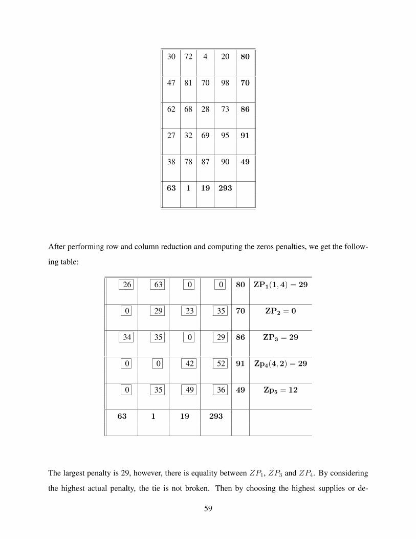
30 72 4 20 80
47 81 70 98 70
62 68 28 73 86
27 32 69 95 91
38 78 87 90 49
63 1 19 293
After performing row and column reduction and computing the zeros penalties, we get the follow-
ing table:
26 63 0 0 80 ZP1(1,4) = 29
0 29 23 35 70 ZP2 = 0
34 35 0 29 86 ZP3 = 29
0 0 42 52 91 Zp4(4,2) = 29
0 35 49 36 49 Zp5 = 12
63 1 19 293
The largest penalty is 29, however, there is equality between ZP1, ZP3 and ZP4. By considering
the highest actual penalty, the tie is not broken. Then by choosing the highest supplies or de-
59
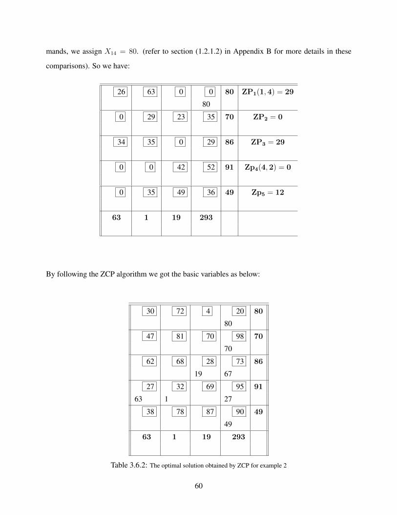
mands, we assign X14 = 80. (refer to section (1.2.1.2) in Appendix B for more details in these
comparisons). So we have:
26 63 0 0 80 ZP1(1,4) = 29
80
0 29 23 35 70 ZP2 = 0
34 35 0 29 86 ZP3 = 29
0 0 42 52 91 Zp4(4,2) = 0
0 35 49 36 49 Zp5 = 12
63 1 19 293
By following the ZCP algorithm we got the basic variables as below:
30 72 4 20 80
80
47 81 70 98 70
70
62 68 28 73 86
19 67
27 32 69 95 91
63 1 27
38 78 87 90 49
49
63 1 19 293
Table 3.6.2: The optimal solution obtained by ZCP for example 2
60

From the tableau 3.6.2, the IBFS of ZCP is the optimal solution of the given problem with the total
cost at $22, 951. Significantly, the optimality reached without additional iterations compared to
VAM and MVM where IBFS is given at $23, 375.
3.7 Computational Experiments
For evaluating the performance of ZCP and MVM, computational experiments were carried out.
The analysis of the experiment data are presented in this section. Again, we run the test on 1600
randomly generated transportation problems. In each case, the values of all cost coefficients, sup-
ply and demand were randomly generated between 1 and 100 for problems of different size. The
test design were implemented using JAVA.
In this comparison the following terms have to be defined:
• The Average Time (AT):
The mean of times consumed to solve problem instances is calculated based on 100 samples
over different sizes.
• The Improvement Rate (IR) :
The average of improvement rate is computed over problem instances for each sizes. This
rate measures the improvement of the solution obtained by both MVM and ZCP comparing
with VAM. Note, It does not include the equality cases of the solutions obtained by VAM.
• The Number of Improved Cases (NIC):
A frequency of both MVM and ZCP when yield to better solutions than VAM
61

Matrix Avg.Time in millisec IR % NIC %size MVM ZCP MVM ZCP MVM ZCP
5 x 5 0.1930 0.3027 0.9360 1.1798 57 56
5 x10 0.2676 0.5958 0.2160 0.9253 41 53
10 x 5 0.3064 0.7288 0.8136 1.1880 63 62
10 x 10 0.3906 0.6890 2.4128 1.9385 80 75
10 x 15 0.4570 1.0102 1.7765 1.7088 71 73
15 x 10 0.4648 1.3044 1.8545 2.8881 70 78
15 x 15 0.6054 1.6657 4.3170 3.939 77 80
15 x 20 0.8443 1.8556 0.8939 0.8450 70 70
20 x 15 0.9259 1.6530 0.4963 1.5775 71 75
20 x 20 0.8822 1.9216 5.9399 6.1476 84 88
25 x 25 1.2797 2.1123 5.5087 5.6069 80 78
35 x 35 1.5591 3.0308 6.4893 5.3806 86 85
50 x 50 1.2580 3.5593 7.720 7.0904 87 84
70 x 70 1.8605 4.7340 6.8199 8.8712 88 89
90 x 90 4.3039 6.9752 9.8814 11.1065 91 96
100 x 100 3.3737 7.3892 9.4109 11.3172 91 91
Table 3.7.1: The Computational Results of MVM & ZCP for Linear Transportation Problems compared to VAM
62
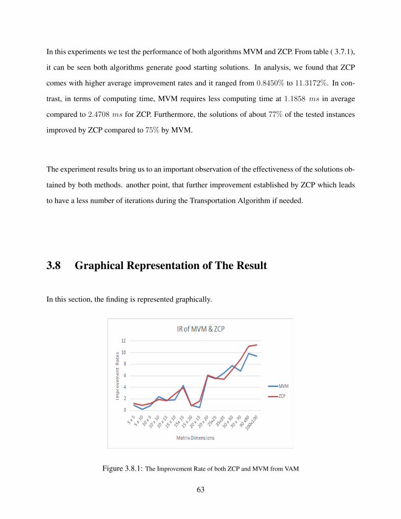
In this experiments we test the performance of both algorithms MVM and ZCP. From table ( 3.7.1),
it can be seen both algorithms generate good starting solutions. In analysis, we found that ZCP
comes with higher average improvement rates and it ranged from 0.8450% to 11.3172%. In con-
trast, in terms of computing time, MVM requires less computing time at 1.1858 ms in average
compared to 2.4708 ms for ZCP. Furthermore, the solutions of about 77% of the tested instances
improved by ZCP compared to 75% by MVM.
The experiment results bring us to an important observation of the effectiveness of the solutions ob-
tained by both methods. another point, that further improvement established by ZCP which leads
to have a less number of iterations during the Transportation Algorithm if needed.
3.8 Graphical Representation of The Result
In this section, the finding is represented graphically.
Figure 3.8.1: The Improvement Rate of both ZCP and MVM from VAM
63
3.9 Conclusion
In this chapter, we have applied new alternate algorithm for solving Transportation problems where
it is shown that this method also gives better initial solutions than VAM. Mainly, comparative study
between the new approach and Modified Vogel method has been established.
Significantly, both ZCP and MVM provide good solutions, in some cases, the optimum for the
Transportation problems. However, ZCP may require more time to run than MVM since each zero
in the matrix is studied individually.
In fact, the procedure of MVM implies more situations to be considered. It is mainly because in
the MVM, we consider the rows and columns penalties. However, in ZCP the penalties of rows
and columns are considered globally on the zero penalties. Therefore, the analysis of the ZCP
algorithm provides less structures. For theses reasons the convergence, if of course it is the case,
with ZCP does seem more probable than MVM.
64

Chapter 4
The Unbalanced Transportation Model
4.1 Introduction
In network flow problems, the unbalanced Transportation model is a special case of The Trans-
portation model where the equality between the total supply and total demand does not hold. In the
real business world, unbalanced transportation problems more likely to find especially when the
total supply exceeds the total demand. Making the right decision may become not an easy task.
Indeed, the objective in this model is to minimize the shipping costs from any source to any destina-
tion without exceeding the supply and demand constraints as a main goal in solving Transportation
Model. In order to establish the goal, this problem need to be transformed into Balanced Trans-
portation problem (BTP). In fact, attempting to balance this Problems and solving them in less
operations, computational time and effort have been the target for many researchers.
In this chapter, a new approach to balance the unbalanced transportation problem (UTP) is in-
65

troduced and a comparison to other existing methods is being carried out. In fact, this approach
was first proposed in [2] and the main concept based on performing the matrix reduction in such
a way that the equivalent cost matrix does not explicitly have a dummy line. Numerical exam-
ples are illustrated in support to our approach and some certain rules are provided to eliminate the
unnecessary calculations.
4.2 Mathematical Formulation of Unbalanced Transportation
Problems
The unbalanced Transportation problem consists of shipping any commodity from any group of
supply centers, called sources, to any group of receiving centers, called destinations, in such a way
the total shipping cost is minimized. Considering a supply ai for each source and demand bj for
each destination where the following condition is not satisfied in this kind of model as
n∑i=1
ai 6=m∑j=1
bj
Mathematically, the Unbalanced Transportation Problem can be formulated as following:
UTP
min TC =n∑
i=1
m∑j=1
Cij Xij
m∑j=1
Xij ≤ ai ; i = 1, · · ·n
n∑i=1
Xij ≥ bj ; j = 1, · · ·m
Xij ≥ 0 ; i = 1, · · ·n ; j = 1, · · ·m
(4.2.1)
Obviously, it is a linear programming with (n×m) variables and (n + m) constraints where Xij
66

represents the amount of commodity shipped from source i to destination j , and Cij is the shipping
cost of one unit form source i to destination j. The first set of the constraints expresses the fact that
the total amount shipped from the source i should not exceed the capacity ai, and the second set
illustrates the fact that the demand at each destination point j should be met. It should be clear that
the constraints in the above formulation are distinct and any node in the network must belong to
only one of the sets to the source or destination sets. Indeed, the objective function is to minimize
the total shipping cost with satisfying the supply restrictions and the demand requirements. Not to
mention, the decision variables Xij take only a positive integer value for all i and j. In fact the
unbalanced case of Transportation models means not all the availabilities will be exhausted, or not
all the demands will be satisfied.
4.3 Analysis & Discussion
The unbalanced version of the Linear Transportation problem has been extensively studied in Op-
erations Research. The process of balancing the UTP has taken several forms so we can classify
those approaches into three main categories.
Heuristics and Meta-heuristics approaches have been used to tackle the problem and some its ex-
tensions to cases with several objectives are considered. For example, Evolutionary Algorithms,
such that Genetic Algorithms [32]. Bee-behavior based algorithms [14] and [12] have been pro-
posed to solve the problems. Search algorithms such that Tabu Search [27] have been also used.
Another Heuristic approach, attempts to balance the problem by getting rid of the redundant which
is the difference between the total supply and total demand [4].
These approaches have in common that they start by finding feasible solutions to the problem then
try to improve them iteratively. Hence, they are impacted by the ease of obtaining such initial fea-
sible solutions.
67

The second category of approaches aims at replacing the unbalanced Transportation problem by
another instance of linear program, and then solve it using the classical simplex algorithm or the
most recent interior points one. We have two types of examples. First, goal programming ap-
proaches have been used to tackle the problem. In this case, if the overall supply is higher than
the overall demand (respectively the overall demand higher than the overall supply), the demands
(respectively the supplies) are considered to be goals that have to be achieved and eventually over-
achieved. A goal programming (GP) (compromise or pre-emptive) problem is then solved using
an appropriate LP solver. Most of the time, this type of approach is also associated with budget
constraints which make the GP even more appealing [25]. Second, some approaches assume that
the unbalance aspects of the transportation problem are in fact the result of uncertainty of the sup-
plies and/or the demands. Hence, some uncertain linear programming method can be used: interval
method [31] and fuzzy linear programming approaches [11] have been applied. Once again, being
able to quickly obtain feasible solutions of the problem will be one of the factors of success.
Finally, the last category attempts to keep the transportation nature of the problem. This is achieved
by using artificial or dummy sources or destinations but they differ in calculating the cost for the
artificial line (row or column). The cost for the dummy is set to equal zero then solved by Vogel
approximation method to find the initial solution [15] or set to a big value as will be defined later
in our approach.
In general, UTP can be divide into two categories: supply exceeds demand, and demand exceeds
supply.
68

• More Supply than Demand
In this case, unbalanced happen when the supply exceeds demand, then
n∑i=1
ai ≥m∑j=1
bj
To balance the problem, we create a dummy (artificial) destination point which satisfies the
following:
bm+1 =n∑
i=1
ai −m∑j=1
bj
To put it differently, that a virtual destination is created with demand equals to bm+1. In the
business world, means we introduce a virtual consumer that would take or consume the sur-
plus offer and the shipments to this consumer are not real.
• More Demand than Supply
In this case, unbalanced happen when the demand exceeds supply, then
m∑j=1
bj ≥n∑
i=1
ai
To balance the problem, we create a dummy (artificial) source point which satisfies the fol-
lowing:
an+1 =m∑j=1
bj −n∑
i=1
ai
In other words, that a virtual source is created with supply equal to an+1. In the business
world, we introduce a virtual supplier that would offer the exact amount of the surplus request
(unmet demand) and again the shipments from this suppler are not real.
After balancing the problem, all the inequalities have transformed into equalities it can be written
mathematically into the following format:
69

BTP
min TC =n∑
i=1
m∑j=1
Cij Xij
m∑j=1
Xij = ai ; i = 1, · · ·n
n∑i=1
Xij = bj ; j = 1, · · ·m
Xij ≥ 0 ; i = 1, · · ·n ; j = 1, · · ·m
(4.3.1)
Where n (n : = n + 1 ) or m ( m := m + 1 ) is a dummy row or column.
Clearly, this artificial source or destination is added to overcome the difference between the avail-
abilities and the requirements. All the approaches used to solve a (balanced) Transportation Prob-
lem (TP), require initial solutions to be computed. The most efficient method, and hence the most
used one, to obtain goods initial TP solutions, is the Vogel’s Approximation Method (VAM). Recall
that the Vogel method find the initial solution by iteratively selecting a pair (i, j) of the source i that
should currently supply destination j as much as possible. This pair is chosen based on the largest
penalty of the sources or destinations, knowing that the penalty of a source (resp. a destination) is
the difference between the two smallest shipping cost at the row (resp. column).
In the tradition approach, that shipping cost from/or dummy line (row or column) takes value of
zero before apply VAM. The disadvantage that it gives inefficient initial solutions by giving the
priority to assign dummy cells before the others.
When the Vogel method is applied to our equivalent balanced TP, the presence of big-M dummy
70

costs make the calculation much more complicated, especially once we start simplex iterations. In
order to overcome this issue, all the applications of the VAM to a balanced TP with dummy sources
or destinations have proposed to ignore totally or partially dummy costs. Hence, Shimshak, (1981-
SVAM [37]) applies VAM while using only the penalties of lines that are parallel to the dummy
line. Goyal, (1984 - GVAM [36]) proposes to replace the big-M by the largest non dummy cost
and fully apply VAM. Balakrishnan, (1990 BVAM [33] ) proposes further modification of SVAM
by calculating all the penalties as the difference between the two smallest non dummy costs. Fi-
nally, Ramakrishnan, (1988 - RVAM [34]) proposes another modification of GVAM which is a
much more complex scheme based on reduction of the all lines parallel to the dummy line, the
replacement of all dummy costs with the largest remaining non dummy cost, before performing
a reduction of all the lines that are orthogonal to the dummy line, including it. This last scheme
seems to provide better solution than the previous approaches on a small number of test problems.
We propose a new approach of the above type where the big-M dummy costs are explicitly taken
into account and are simply eliminated during the process. Our approach is based on the Modified
Vogel Method (refer to chapter 2). It allows us to obtain an equivalent balanced TP obtained while
taking explicitly into account dummy costs.
4.4 New Approach for Transforming UTP to BTP
As defined earlier, in the process of balancing the TP, a dummy supply or demand is added to the
cost matrix to satisfy the equality. In our approach, the cost values at the dummy row or column
are given value M which should be large enough to discourage sending or receiving commodities.
Then after balancing the problem, we apply MVM. As defined, the cost reduction starting by either
row or column must be performed as a first step in modified Vogel algorithm. However, in this case
we need to pay more attention to whether start with row or column reduction. If a dummy row is
71

added then a column reduction would be as first step then the row reduction. Likewise, in case of a
dummy column, a row reduction must perform first.
• In the Dummy Source
The cost value at that row takes the value
Cn+1,j = M, ∀ j = 1, · · ·m
In this case the dummy line is a row, we set dummy= n+1 and the reduction has to start with
the columns first then the rows. Otherwise, the cost at the dummy row turns to zeroes since
the coefficients associated to the dummy row are all equal to a sufficiently large M. Therefore
the dummy row will be reduced after performing the row reduction. That reduction make the
value M to disappear from the reduced matrix.
Therefore any value of M can be used if we avoid choosing the least cost on the dummy row.
• In the Dummy Destination
The cost value at that column takes the value
Ci,m+1 = M, ∀ i = 1, · · ·n
In this case the dummy line is a column, we set dummy=m+1 and we have to reduce the rows
first then the columns. Otherwise, the cost at the dummy column turns to zeroes since the
coefficients associated to the dummy column are all equal to a sufficiently large M. Therefore
the dummy column has to be reduced after we perform the column reduction. That reduction
makes the value M to disappear from the reduced matrix.
Therefore any value of M can be used if we avoid choosing the least cost on the dummy
column.
72

4.4.1 Common Best Cases
In this subsection, we discuss situations where the minimum costs of the first reduced lines (rows
or columns) are all the same.
Dummy Column
In this case, the rows are reduced first with their minimum costs being equal. The reduction of the
dummy column leads to all its reduced cost equal to zero. Therefore, the penalties of rows become
all equal to zero since each row will have at least two zeroes: one at the location of the original
minimum cost and the second one in the dummy column. The only possible non null penalties
would be on the non-dummy columns. Then we have two situations. The first corresponds to the
case where the largest penalty is not null while the second is associated with a null largest penalty.
Case 1: No Null Penalty
The only non-null penalties are among the columns. We assign successively the columns associ-
ated to a non-null penalty until all the penalties of the remaining column are equal to zero. Then
we re-evaluate the penalty of the rows. If the penalties of the rows are all null then the situation is
described in case 2. In the other case there at least one row having a non- null penalty. Therefore
we can continue the algorithm.
Case 2: Null Penalty
In this case, all the penalties are null we can use the least cost algorithm to solve the problem.
We use the fact that the lowest costs of the rows are equal to the same value. We can assign
simultaneously these zero independent. Then we cross out the row or column with no supply or
demand.
73
Dummy Row
In this case the columns are reduced first with their minimum costs being equal. The reduction of
the dummy row implies all its reduced cost equal zero. Therefore the penalties of columns become
all equal to zero. The only possible non null penalty would be on the other rows. Then we have
two situations. The first corresponds to the case where the largest penalty is null while the second
is associated to a no-null largest penalty. These situations are similar to the cases described in the
preceding subsection. The roles of the columns are replaced the ones of the rows.
A certain number of rules are provided to eliminate the need to recalculate a new reduced cost
matrix for the whole remaining table.
4.5 MVM Algorithm
The following is the matrix reduction procedure for Unbalanced Transportation problem which dif-
fers than the case of Balanced Transportation problem.
General Algorithm
Step 1. Balancing the Problem
If A Dummy Row n is added then
Go to step 3
else
Go to step 2
74

Step 2. Row-Column Reduction
∀ i Find ui = minj{Cij} then set Cij = Cij − ui ; j = 1, · · · ,m
∀ j Find vj = mini{Cij} then set Rij = Cij − vj ; i = 1, · · · , n
Step 3. Column-Row Reduction
∀ j Find vj = mini{Cij} then set Cij = Cij − vj ; i = 1, · · · , n
∀ i Find ui = minj{Cij} then set Rij = Cij − ui ; j = 1, · · · ,m
At this stage Set NRed = 1 (Indicate the Number of Reductions for the matrix)
Step 4. Applying MVM
Then apply MVM for the reduced matrix by starting with the penalty calculations and then
continue with the process.
It is important to realize with this approach of balancing the problem, the dummy aspect is no
longer explicitly present. Therefore this yields to a BTP which can be solved by either MVM
or ZCP, and there proceeding results for the LTP can be applied to this problem after using the
balancing approach.
4.6 Example of Illustration
We shall consider the problem was introduced in [37] and solved by many researchers as [36] , [34]
and [33]:
75

1 2 3 SP
A 6 10 14 50
B 12 19 21 50
C 15 14 17 50
DM 30 40 55
The initial solution is 1745 by Vogel’s Approximation Method:
6 10 14 0 50
40 10
12 19 21 0 50
30 20
15 14 17 0 50
25 25
30 40 55 25
Table 4.6.1: The initial solution obtained by VAM for UTP
The initial solution is 1695 by Shimshak’s Modified Method:
6 10 14 0 50
30 20
12 19 21 0 50
25 25
15 14 17 0 50
20 30
30 40 55 25
Table 4.6.2: The initial solution obtained by SVAM for UTP
76

The initial solution is 1665 by Goyal’s Modified Method:
6 10 14 21 50
40 10
12 19 21 21 50
30 20
15 14 17 21 50
45 5
30 40 55 25
Table 4.6.3: The initial solution obtained by GVAM for UTP
The initial solution is 1650 by Ramakrishnan’s Method:
6 10 14 9 50
5 40 5
12 19 21 9 50
25 25
15 14 17 9 50
50
30 40 55 25
Table 4.6.4: The initial solution obtained by RVAM for UTP
The initial solution is 1650 by Balakrishnan’s Modified Method:
77

6 10 14 0 50
5 40 5
12 19 21 0 50
25 25
15 14 17 0 50
50
30 40 55 25
Table 4.6.5: The initial solution obtained by BVAM for UTP
Now try to find the solution by MVM. In the following table, a virtual destination is added to the
problem to satisfy the balance condition.
1 2 3 Dummy SP
A 6 10 14 M 50
B 12 19 21 M 50
C 15 14 17 M 50
DM 30 40 55 25
The reduced matrix cost after performing the row then the column reduction implies the following
equivalent matrix:
78

1 2 3 Dummy SP
A 0 4 6 9 50
B 0 7 7 3 50
C 0 0 0 0 50
DM 30 40 55 25
Obviously, the matrix does no longer have the dummy aspect. Then continue by applying MVM.
6 10 14 M 50
5 40 5
12 19 21 M 50
25 25
15 14 17 M 50
50
30 40 55 25
Table 4.6.6: The initial solution obtained by MVM
The total cost is 1650, which in fact the optimal.
4.7 Computational Test
To illustrate our approach further, we did the following experiment on 100x10 randomly generated
unbalanced transportation problems. The cost coefficients as well as supply and demand values are
distributed between 1 and 100.
79

Matrix IR % NICsize BVAM RVAM MVM BVAM RVAM MVM
5 x 5 -3.9461 6.1534 9.6225 20 65 79
5 x10 -18.2643 12.8477 15.1760 29 75 83
10 x 5 -24.7193 10.3684 14.1223 24 73 83
10 x 10 -4.7274 9.0171 12.2014 21 72 85
10 x 15 -6.2745 18.4432 20.8484 35 82 90
15 x 10 -8.1456 17.3828 21.125 32 86 92
15 x 15 -5.1838 9.0831 12.5156 15 70 80
15 x 20 -4.6008 18.1938 20.8842 35 87 93
20 x 15 -5.6086 16.6715 19.5103 30 83 92
20 x 20 0.6854 13.6854 15.9065 39 78 88
25 x 25 -0.815 13.6163 19.1398 30 78 91
35 x 35 -0.6673 10.0586 18.1335 27 71 90
50 x 50 -3.079 8.9345 16.7347 24 75 91
70 x 70 -0.684 10.9717 19.1653 39 75 95
90 x 90 0.3467 11.5076 19.3165 33 76 93
100 x 100 -0.6703 9.631 16.9191 35 75 89
Table 4.7.1: The Computational Results for Unbalanced Transportation Problems
80

The comparison to VAM, SVAM, GVAM and BVAM were made to the potential significant of the
proposed approach. The results shown in table (4.7.1). As defined earlier, IR refers to the average
of improvement rate for 100 problems instances at each size while NIC for the number of improved
cases comparing to VAM.
The experiment results bring us to an important observation of the effectiveness of the solutions
obtained by MVM. In analysis, we found that the more efficient solutions are obtained by MVM. It
is important to point out that this efficiency of MVM comes with the general average improvement
rate at 16.96% compared to 12.29% for RVAM while there is no improvement for BVAM at the
average −5.4%. In addition, the statistical standard errors have been computed at 0.01725 , 0.0094
and 0.0086 for BVAM , RVAM and MVM respectively.
4.8 Graphical Representation of the results
In this section, the findings is represented graphically.
Figure 4.8.1: The Number of Improved Cases for BVAM, RVAM and MVM
81

Figure 4.8.2: The Average Running Times of BVAM, RVAM and MVM for different-sized instances
Figure 4.8.3: The Average Improvement Rates of BVAM, RVAM and MVM for different-sized instances
4.9 Conclusion
In this chapter, a new approach is presented to solve the Linear Unbalanced Transportation Problem
without dealing explicitly with a dummy line. The reduction of the matrix provides an equivalent
82

matrix which no longer has the dummy aspect. Then one of the presented methods in this thesis
can be applied, Modified Vogel method (MVM), or Zero Case Penalty algorithm (ZCP), to solve
the resulting transportation problem. A certain number of rules are provided to eliminate the need
to recalculate a new reduced cost matrix for the whole remaining table.
In some cases, simultaneously a bundle of variables are assigned. Important to realize, in the
case where all the reduced cost were zeroes, it provides the optimal solution. It also allows the
identification of the optimal solution whenever the reduced cost equals to zero. Consequently this
avoids, in these cases, the use of the transportation algorithm.
83

Chapter 5
The Transshipment Model
5.1 Introduction
Transshipment Problems have lately gained more attention in several fields particularly with those
related with allocation or supply chain system. Transshipment model is an extension of Trans-
portation Problem where transit points exist and with the possibilities of shipping within sources
and within destinations.
In general, the Transshipment Problem consists in shipping a commodity from supply centers,
called sources, to receiving centers, called destinations where the shipments pass through interme-
diate points. Instances of problem arise in distribution networks where goods are shipped from
large warehouses to retails stores, either directly or through smaller and specialized warehouses
called cross-docking terminals [16], [23] & [15]. Transshipment Model is more realistic and more
difficult to deal with than the Transportation model since it does not deal only with direct paths for
each origin-destination pair but also with paths that go through junction points also called trans-
shipment points.
84

This type of model exists when there is a need to ship via transit points before reaching the final
destination whether will be less costly or/and less time consuming.
Similarly to the Transportation model, the object here is to minimize the total cost of shipping units
from all the sources to all final destinations. Clearly, the goal is to determine the quantities that
need to be transported from a set of sources to a set of destinations via a set of transition points
with satisfying the supply and demand constraints.
Furthermore, the Transshipment Model has three groups of nodes as illustrated below:
• Source nodes:
Usually source nodes have output arcs and they provide positive supply and have zero de-
mand. These type of nodes are called pure sources. In the Transshipment model, however,
there exist another source node that could be a transit point as well when there are input arcs
and is referred to as a Transit-source node.
• Pure Transshipment points:
They provide zero supply and have zero demand. In another word, these nodes have non-zero
in-degree and out-degree.
• Destination nodes:
Generally, destination nodes have input arcs and they have positive demand and provide zero
supply. These type of nodes are called pure destinations. In the Transshipment model, a
destination node could be also a transit point with output arcs and is referred to as a transit-
destination node.
85

Generally, this type of problem is solved after reformulated into regular Transportation model by
considering all the source and the destination points. In some cases, solving Transshipment prob-
lems may become more complicated by adding buffer values. In this thesis, our approach for
solving this model is to find the lowest-cost path for each source-destination pair. However, the
least-cost routes are unknown in advance for this type of problem. In fact, define these routes is not
an easy task and an appropriate algorithm should be chosen wisely. Furthermore, the minimum-cost
routes from one supply center to another receiving center may be direct or pass through intermedi-
ate transfer points. The intention in the proposed approach is to reduce the Transshipment models
to Transportation problem by using Floyd algorithm to find the shortest path and these paths be-
come the costs for TP.
After reformulation of the initial Transshipment problem into an easy-to-solve Transportation prob-
lem, the Modified Vogel method which mentioned into a detail in the previous chapter can be ap-
plied to find the optimal solution. Numerical examples are illustrated to show the usefulness of this
approach.
5.2 Formulation of Transshipment Problems
5.2.1 Network Representation
The Transshipment model can be defined as a network G = (N,A) where the set N is constituted
by all the nodes while A is the set of the existing links between these nodes. It can be defined by
the set A as {(i, j), i, j ∈ N} where N = {1, 2, · · ·L} ,with L = n+m+ t.
Assuming that we have n different sources in the set S = {1, 2, · · ·n}, m different destinations
in the set D = {1, 2, · · ·m} and t pure transshipment points in the set T = {1, 2, · · · t}. The unit
cost for shipping from the source i to destinations j is denoted by Cij . This allows the network
86

representation of the Transshipment problem as:
s1
s2
t1
t2
d1
d2
sn tr dm
Figure 5.2.1: The Transshipment Network
5.2.2 Mathematical Representation
Generally, the Transshipment Problem (TSHP) can be formulated as:
TSHP
min TC =∑
(i,j)∈ACij Xij
∑k/(i,k)∈A
Xik −∑
k/(k,i)∈AXki = ai ; i ∈ S
∑k/(k,j)∈A
Xkj −∑
k/(j,k)∈AXjk = bj ; j ∈ D
∑k/(k,r)∈A
Xkr −∑
k/(r,k)∈AXrk = 0 ; r ∈ T
Xij ≥ 0 ; (i, j) ∈ A
(5.2.1)
87
In the above model, Xij represents the amount of commodity shipped from node i to node j, the
first set of the constraints expresses the fact that the total amount shipped from the source i should
not exceed the capacity at i, and the second one means that the demand at destination j should be
met. Finally the third set of constraints illustrates the fact that no commodity remains at the transit
or junction points which means all commodities flow through these junction points.
Clearly, TSHP is a linear programming which could be solved by any specialized simplex method.
Note that in the classic transportation problem, no junction nodes exist and the above model can be
easily adapted. The sources could receive units for another source and act as transit points. Simi-
larly, the units can be shipped from destinations to other nodes and to act as transit points. So the
supply and demand constraints must be adjusted.
As mentioned earlier, solving this model it can be done by converting the problem into a Trans-
portation form. In the third section, we will discuss in details how to deal with this type of problem
and solve it in our approach and how to calculate the cost matrix. Therefore, several of the ap-
proaches that have been developed to tackle the Transshipment Problem consist in reformulating
into an equivalent Transportation Problem. This approach generally recognizes the relation be-
tween the unit amounts and the total cost of any route.
It is essential to highlight the fact that several kinds of transshipment models with very special
properties exist. Due to their properties, our approach can be applied with the need of considering
the special properties. Capacitated Transshipment problem, for instance, is a type that requires
having a logical maximum and minimum bounds on the shipment of each route. So, the object
is not only to minimize the shipping cost but also to meet the demand requirements with supply
availability without exceeding the lower and upper bounds. As the scope of this thesis, in this
chapter we only discuss the general Transshipment model.
88

5.3 Transportation Algorithm for TSHP Problems
The concept of Transshipment Problems have been introduced and discussed in several papers and
textbooks by many researchers in the field of Mathematics and Operations Research [15], [23], [24]
and [7]. In this section, some of the previous methods need to be mentioned to give a necessary
background on this type of problem and how the TSHP is solved. This model can be translated
into Transportation model to solve with Transportation algorithm but the presence of transit points
makes the process complicated. However, in the field of optimization problems, alternative ap-
proaches exist in how to construct this model into a regular Transportation form.
This approach consists in considering all the nodes (source, destination and transit nodes) as both
source and destination points in the Transportation tableau in order to have always a square matrix
([7]-chapter4). So we obtain a transportation model with n + m + t sources and n + m + t
destinations where the supply and demand for the transit points are equal to total supply or demand.
While the supply value for destinations and the demand value for sources equales to zero. In addi-
tion, source nodes (respectively destination nodes) that were sources (respectively destinations) in
the Transshipment Problem keep the same capacity (respectively demand).
Another method is a buffer method which is the most common method for completing the trans-
formation of the problem into a regular Transportation model based on the concept of a buffer.
Basically, this method handles the transshipment points as sources and destinations at the same
time. Further, if any source acts as transit-source node should be added as well to the destinations
in the transportation table. Similarly, if any destination acts as transit-destination node should be
added as well to the sources in the transportation table. Consequently, each transit point has special
demand and supply variables to convert the problem into Transportation model.
89

The basic idea is to consider any node that receive and ship commodity as a transshipment point
regardless of it being originally a source, destination or a transit node [15]and [13]. The exact
quantities of product that will pass through the transit points are unknown. So, by calculating a
stock buffer value B we can add it as supply and demand values for the pure transshipment points.
B is added to balance the problem and it can be equal to the sum of the supply or to the sum of the
demand and should be large enough to allow the units pass through these intermediate nodes. A
stock buffer value B is then calculated using the original demands and capacities in order to balance
the problem. It is usually equal to the sum of capacities or the sum of demands.
Then, each pure transshipment point is assigned a capacity and a demand equal to B when each
transit-source point, the demand value is equal to the sum of B and its original capacity. Likewise,
for each transit-destination point, the supply value is equal to the sum of B and its original demand.
Briefly, demand and supply can be defined as:
B
Si = Di = B ; i ∈ Pure Transshipment Points
Si = B + s , Di = B ; i ∈ Source− Transit Points
Si = B , Di = B + d ; i ∈ Destination− Transit Points
Si = s , Di = d ; i ∈ Pure Source or Destination points
(5.3.1)
Furthermore, the cost matrix has arbitrary large number M for cost of non-exited routes and zero
cost of circle routes. M is selected to be sufficiently large to ensure that the algorithm avoid assign-
ing to these routes as much as possible. After that, the Simplex Transportation Algorithm is just
used to the cost matrix in order to get optimal solution.
90

In both approaches, the equivalent Transportation Problem is solved using transportation simplex.
However, in practice, solving this instance of transportation model is complicated due to the fact
that the equivalent problem is large in size, have at the same time unit cost equal to 0 and big M.
Consequently, needless computations are made to include non-existent routes in the Transportation
problem with cost M . In practice, this value serves no purpose in determining an optimum in this
type of problem.
5.4 Reduction to Smaller Transportation Model
In many applications, the process of formulating this type of problem can get more complicated
where we have to deal with hundreds or thousands of source, destination or transit points. It would
not be effective, as expected, since we are increasing the dimension of the problem by adding the
transshipment points as sources and destinations. The technique here, which was first introduced
in [1], is to solve Transshipment problem by Modified Vogel Method MVM after formulating the
problem in a context of transportation model with considering the minimum-cost route between
each source and destination. The number of sources and destinations remains the same as in the
original problem and that route would be either direct or indirect through a series of points.
Basically, the motivation of this approach is not to create only a transportation problem from the
Transshipment problem but to avoid including the transit points into the network model. In other
words, that means we would have reduced Transportation model instead of complex one which
also depends on the number of intermediate nodes. Obviously, the amount of computation will be
reduced by having a smaller Transportation problem.
Indeed, our equivalent problem has as many sources (resp. destinations) as the original Trans-
91
shipment problem. Choosing the minimum-cost route between each source and destination can
be analyzed and formulated by using Floyd Algorithm which based on Graph Theory. In the fol-
lowing section, the function of Floyd Algorithm will be demonstrated and how can be applied in
our approach. consequently, the result transportation problem has the same sources and the same
destinations at the original problem where the direct links are the minimum cost paths obtained
from the Floyd Algorithm. Finally, we apply the Modified Vogel Method to obtain optimal or near
optimal solutions to the problem.
Needly to mention, while there are several algorithms based on graph theory that can eliminate the
transit points in order to determine the shortest paths, we find Floyd algorithm is the best suited
for our needs. Specifically, in our approach, the technique of Floyd algorithm allows us to keep
track of the intermediate nodes in an informative matrix during the process of determining the least-
cost path linking every source-destination pair. Dijkstra and Bellman algorithms are examples for
methods that solve shortest path problems. Generally, Dijkstra used to find the shortest path from
a single node to another. So, if we want to find the shortest path for the network model we need to
consider each node as starting node. Whereas, Bellmans algorithm finds the shortest route back-
ward from the destination to each source. In fact, an additional work is needed to determine the
shortest path for each destination and to keep track of all the paths at the end.
In the resulting model, the cost represented between each source and destination is associated to
a route that could be directed or undirected in the initial Transshipment model. Beside to the cost
or distance matrix in the Transshipment model, a P (revered to path) matrix is generated by Floyd
algorithm to facilitate the retracting of all the determined least paths once the solution is obtained.
Obviously, determining the right least-path algorithm is an educated choice to make a fundamental
contribution in terms of calculation time and efficiency.
92

5.4.1 Floyd Algorithm
As stated previously, the path that corresponds to each route in the new model needs to be recog-
nized in order to translate the solution to a solution that fits the initial problem. For that reason,
Floyd algorithm is a good choice. This algorithm is more effective to deal and find the shortest path
between every two nodes in the whole network. This network will be represented as informative
square matrices.
Let’s denote D for the Distance matrix and P for the path matrix, where D gives the distance or
cost between node i and j for all i, j = 1, · · ·n and it could be finite if the link exist and infinite
otherwise. Where the matrix P illustrates the path included transit node if exist between each node
i and j. The diagonal elements in both matrices are blocked and could take zero value. Note that an
undirected path could consist a single transit point or a series of intermediate points.
Assuming that the network problem is presented with n nodes, so the D matrix n x n, first created
based on the initial cost (weight) of the path between each node i and j as following:
dij =
0 ; if i = j
w(i, j) ; if i 6= j , (i, j) ∈ A
∞ ; if i 6= j , (i, j) /∈ A
(5.4.1)
And the P matrix initially created with all the elements are equal to zero since there is no interme-
diate node at this step. The following procedure describe how the Floyd algorithm is applied to the
Transshipment problem.
93
Floyd Algorithm
Step 1. Define D & P Matrices
Define the Distance matrixD and the Path matrix P from the Network. Both matrices are square
with n rows and n columns. In D matrix, its elements dij are the distance between the node i and
j and take finite value if the link exist and infinite otherwise. In P matrix, its elements pij are the
intermediate node between the node i and j but initially these elements are zeros.
Step 2. Pivot
Starting the pivot k when k = 1, · · ·n
Define the row and column pivot then apply the Triple Operation to each element in the D ma-
trix except the ones on the row and column pivot.
The Triple Operation equation is defined in the following form:
dik + dkj < dij where i 6= k, j 6= k and i 6= j. If that condition is satisfied then replace dij with
dik + dkj in D matrix.
Step 3. Determine the Shortest Routes & Update P matrix
In P matrix, replace the element at the position i, j with k at the kth iteration.
Step 4. Stop Case
If k = n+ 1
stop
else
k := k + 1
94
Step 5. Read form Both D and P matrices
In D matrix, dij gives the cost of the shortest path between node i and node j. While, in P
matrix, the element pij yields the transit point between the node i and node j. If the node j is not
the final destination then continue the procedure between the node at the position ij to the node j.
At first, we look at each source and destination in order to calculate the lowest-cost path. Basi-
cally, the technique is to apply the algorithm to each source and then determine the least path to
each destination. Certainly, the algorithm will run for kth time where k is the number of transship-
ment points, whether they are pure transit, transit-source, or transit-destination nodes. Generally,
Floyd algorithm run for n nodes with time complexity O(n3).
In the output matrices, D returned the new cost between each node and P matrix provides all
the necessary information about the transit point if existed between each source and destination
in order to retain the initial path. So the element at position (i, j) at matrix P is either 0 or any
number between 1 and n. In the case of non-zero element, h for instance, means the path from i
to j containing the node h. which in another word there is a subpath from i to h and an another
subpath from h to j.
In our approach, both matrices D and P have the dimension L , where L = n+m+ t .
Remark:
In the Transshipment model, the Floyd Algorithm would be in the best case scenario. Since we start
with upper triangular matrix D with∞ under the main diagonal, the row or column corresponding
to the pivot element∞ would not be considered in the triple operation where this allows to speed
up the algorithm.
95

5.4.2 General Algorithm
In this section, the steps involved in execution of the proposed method are outlined as following:
Reduction Algorithm
Step 1. Cost matrix Calculation
Determine the cost matrix C by conducting the Floyd Algorithm on the Transshipment problem.
The dimension of the cost matrix will be n x m and the shipping cost between each source i and
destination j will be the minimum cost in the rout ij.
Balance the problem if the equality between the supply total and the demand total does not hold.
Step 2. Apply MVM
Apply MVM to the cost matrix. Start by performing Row and Column reductions then evaluate
the row and column penalties.
Step 3. Solution Transformation
Translate the solution obtained in the previous step to fit the initial Transshipment problem.
The assigned variable for the TP is Ysi,dj = h, ∀i, j. Then the corresponding assignment variable
to the Transshipment problem is determined as follows:
xsi,pl1 := xsi,pl1 + h , xpl1 ,pl2 := xpl1 ,pl2 + h , · · · · · · , xplr ,dj := xplr ,dj + h , plr ∈ L
96

5.5 Examples of Illustration
In this section, the procedure of the algorithm is illustrated by the following problems.
5.5.1 Example 1
DA
Htn
Chgo
LA
SF
NY
929
14
13
16
27
26
17
18
7 15
17
Figure 5.5.1: The Transshipment network of example 1
A company manufactures a product in Dallas and Houston. The daily capacities at Dallas and
Houston are 160 and 200 respectively. Products are shipped by air to customers in San Francisco
and New York. The customer’s daily needs at both cities are 140 units. Because of the deregulation
of air fares, it may be a cheaper to the company to fly to transit points then to the final destinations.
Chicago or Los Angeles could be the transit cities. The costs per unit between the cities are shown
in the network (5.5.1). The company wants to minimize the shipment costs for daily required prod-
ucts.
97

Apply Floyd Algorithm to determine the least path from the origin 1 and 2 to all the destinations 6
and 7. The steps are illustrated as following:
STEP 1. Based on the initial network, we define the D matrix:
DA Htn Chgo LA SF NY
DA 0 ∞ 9 14 ∞ 29
Htn ∞ 0 16 13 27 26
Chgo ∞ ∞ 0 7 17 18
LA ∞ ∞ ∞ 0 15 17
SF ∞ ∞ ∞ ∞ 0 ∞
NY ∞ ∞ ∞ ∞ ∞ 0
and P matrix:
DA Htn Chgo LA SF NY
DA 0 0 0 0 0 0
Htn 0 0 0 0 0 0
Chgo 0 0 0 0 0 0
LA 0 0 0 0 0 0
SF 0 0 0 0 0 0
NY 0 0 0 0 0 0
98

STEP 2: Starting the Floyd iterations:
Iteration: 1
Set the pivot k = 1, so the first row is the pivot row and the first column is the pivot column. Then
shade the first row and first column, and check for improvement by applying the triple operation.
Iteration: 2
Set k = 2 , there are no changes.
Iteration: 3
Set k = 3 , cell (1,5) changes to 26 and (1,6) changes to 27.
After finding a shorter path, we need to update P matrix in order to tell that k = 3 provides
the shortest path between the source 1 and destination 5 as well as between the source 1 and the
destination 6.
Iteration: 4
Set k = 4 , there are no changes.
Iteration: 5
Set k = 5, there are no changes.
Iteration: 6
Set k = 6, there are no changes. At the end, the result matricesD and P have the following values.
99

DA Htn Chgo LA SF NY
DA 0 ∞ 9 14 26 27
Htn ∞ 0 16 13 27 26
Chgo ∞ ∞ 0 7 17 18
LA ∞ ∞ ∞ 0 15 17
SF ∞ ∞ ∞ ∞ 0 ∞
NY ∞ ∞ ∞ ∞ ∞ 0
Table 5.5.1: The Cost Matrix after using Floyd algorithm
DA Htn Chgo LA SF NY
DA 0 0 0 0 3 3
Htn 0 0 0 0 0 0
Chgo 0 0 0 0 0 0
LA 0 0 0 0 0 0
SF 0 0 0 0 0 0
NY 0 0 0 0 0 0
Table 5.5.2: The Path Matrix after using Floyd algorithm
STEP 3: In this step we rewrite the problem in a transportation format with the help from the
Floyd algorithm. We get :
100

SF NY Sp
DA 26 27 160
Htn 27 26 200
Dm 140 140
Table 5.5.3: The result Transportation tableau for example 1
STEP 4: Now we just apply MVM to the previous problem to get the optimal solution or at least
near to optimal solution.
The process for balancing the problem is needed since the supplies exceed the demands. So we get:
SF NY Dummy Sp
DA 26 27 M 160
Htn 27 26 M 200
Dm 140 140 80
After apply MVM, we have:
101

SF NY Suuply
DA 26 27 160
140
Htn 27 26 200
140
Demand 140 140
Table 5.5.4: The solution by MVM for example 1
Based on the previous table, we can determine the assignment variables for the initial transship-
ment problem.
Since YDa,SF = 140 and the shortest path from Dallas to San Francisco being defined byDallas→
Chicago→ SF then
XDa,Chgo = 140 and XChgo,SF = 140
Since YHtn,NY = 140 and the shortest path from Houston to New York being the direct path then
XHn,NY = 140
The resulting network based on the reduction approach is shown below:
102

DA
Htn
Chgo
LA
SF
NY
9
26
17
Figure 5.5.2: The network representation of the solution to the Transshipment problem 1
5.5.2 Example 2
In this example, we shall apply our technique to a problem was introduced in [23]. The transship-
ment problem consist three sources, five transit points and four destinations. In their text, they
transformed the problem into a Transportation problem and the resulting was 12× 12 matrix (table
5.5.6) which becomes too large to solve according to their views. The objective function is to de-
termine the routes and allocation of units which will minimize the total cost.
In comparison, in our approach the resulting Transportation problem would be 3× 4. The determi-
nation of the shortest paths for each source-destination pair can be done be Floyd algorithm.
103

to Cannery Junction Warehouse
From 1 2 3 4 5 6 7 8 9 10 11 12 supply
Cannery
1 0 146 − 324 286 − − − 452 505 − 871 75
2 146 0 − 373 212 570 609 − 335 407 688 784 125
3 − − − 658 − 405 419 158 − 685 359 673 100
Junction
4 322 371 656 0 262 398 430 − 503 234 329 −
5 284 210 − 262 0 406 421 644 305 207 464 558
6 − 569 403 398 406 0 81 272 597 253 171 282
7 − 608 418 431 422 81 0 287 613 280 236 229
8 − − 158 − 647 274 288 0 831 501 293 482
Warehouse
9 453 336 − 505 307 599 615 831 0 359 706 587
10 505 407 683 235 208 254 281 500 357 0 362 341
11 − 687 357 329 464 171 236 290 705 362 0 457
12 868 781 670 − 558 282 229 480 587 340 457 0
Demand 80 65 70 85
Table 5.5.6: The Transportation tableau of Transshipment example 2
104
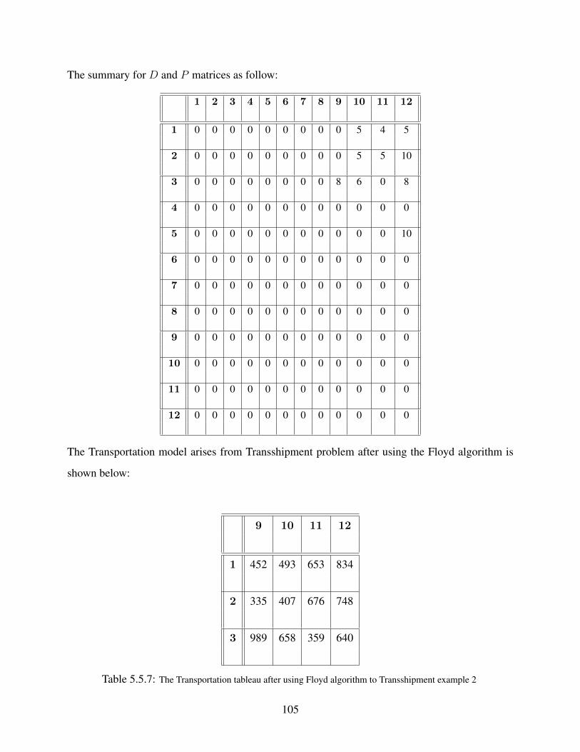
The summary for D and P matrices as follow:
1 2 3 4 5 6 7 8 9 10 11 12
1 0 0 0 0 0 0 0 0 0 5 4 5
2 0 0 0 0 0 0 0 0 0 5 5 10
3 0 0 0 0 0 0 0 0 8 6 0 8
4 0 0 0 0 0 0 0 0 0 0 0 0
5 0 0 0 0 0 0 0 0 0 0 0 10
6 0 0 0 0 0 0 0 0 0 0 0 0
7 0 0 0 0 0 0 0 0 0 0 0 0
8 0 0 0 0 0 0 0 0 0 0 0 0
9 0 0 0 0 0 0 0 0 0 0 0 0
10 0 0 0 0 0 0 0 0 0 0 0 0
11 0 0 0 0 0 0 0 0 0 0 0 0
12 0 0 0 0 0 0 0 0 0 0 0 0
The Transportation model arises from Transshipment problem after using the Floyd algorithm is
shown below:
9 10 11 12
1 452 493 653 834
2 335 407 676 748
3 989 658 359 640
Table 5.5.7: The Transportation tableau after using Floyd algorithm to Transshipment example 2
105

The next tableau shows the basic feasible solution which was determined by using Modified Vogel
Method. Notice this technique provides an optimal solution.
9 10 11 12 Supply
1452 493 653 834 160
65 10
2335 407 676 748 125
80 45
3989 658 359 640 100
70 30
Demand 80 65 70 85
Table 5.5.8: The Transportation solution tableau for example 2 after using MVM
The total cost is $ 145,175
It is an optimal solution for both the transportation problem and the transshipment problem. From
the previous tableau and P matrix, we can determine the assignment variables and retain the path
for the initial transshipment problem.
Since Y1,10 = 65 and the shortest path from source 1 to destination 10 being defined by 1→ 5→ 10
then
X1,5 = 65 and X5,10 = 65
Since Y1,12 = 10 and the shortest path from source 1 to destination 12 being defined by 1 → 5 →
10→ 12 then
106

X1,5 := X1,5 + 10 = 75 , X5,10 := X6,10 + 10 = 75 and X10,12 = 10
Since Y2,9 = 80 and the shortest path from source 2 to destination 9 being defined by the direct
path 2→ 9 then
X2,9 := 80
Since Y2,12 = 45 and the shortest path from source 2 to destination 12 being defined by 2→ 10→
12 then
X2,10 = 45 and X10,12 := X10,12 + 45 = 55
SinceY3,11 = 70 and the shortest path from source 3 to destination 11 being defined by the direct
path 3→ 11 then
X3,11 := 70
Since Y3,12 = 30 and the shortest path from source 3 to destination 12 being defined by 3→ 8→ 12
then
X3,8 = 30 and X8,12 = 30
The resulting network based on the reduction approach is shown below:
107

1
2
3
4
5
6
7
8
9
10
11
12
75
505
80
45
30
70
75
30
55
Figure 5.5.3: The network representation of the solution to the Transshipment problem 2
5.6 Conclusion
In this chapter, we studied the Transshipment models which have a relation on the general feature
with the Transportation models. The reductive approach which provides interesting advantages
over the existed methods for solving the Transshipment problems, have been proposed.
Arising a small and less-complex Transportation model from the initial Transshipment model is the
best advantage of the proposed method compared to virtually unsolvable problem that the buffer
method would produce. The Floyd algorithm provides a clear view of the turning process to Trans-
portation problem since it is a matrix-based algorithm. Another key point, that the result Trans-
portation problem can be solved by one of MVM or ZCP algorithms that we introduced in this
thesis.
108

Chapter 6
Application to the Traveling Salesman
Problems
6.1 Introduction
The Traveling Salesman Problem (TSP) is widely studied by many researchers in the field of Math-
ematics and Computer science. In terms of Combinatorial Optimizations, TSP falls in the category
of NP-complete problems and play an important role in Operations Research and theoretical Com-
puter science.
In general, TSP has several practical applications, which extends beyond the definition of cities
and distances, in business, industry and engineering. In fact, several heuristic algorithms have been
applied to solve TSP. The primary goal is to find the optimal tour that minimize the total distances
or the required costs.
109

In this thesis, we present a new heuristic algorithm for the traveling salesman problem. It uses
the Modified Vogel Method (MVM) to improve one of the effective heuristic algorithm, the near-
est neighbor algorithm. It also has the potential of being a convergent algorithm in some cases.
Numerical examples will be considered to illustrate the procedure.
6.2 Traveling Salesman Problem
In the graph theory, Traveling Salesman Problem (TSP) is stated as a complete graph G = (N,E)
where N is a set of nodes {1, 2, · · ·n}, and E is a set of edges {(i, j) = eij , i, j ∈ N}. while
the distance or cost (as represented in this chapter) cij corresponding to each edge eij . Generally,
the nodes represent cities and the edges represent the distance between the cities. The goal is to
find the lowest cost or the shortest path tour T between n cities. In terms of graphs, it is to find the
Hamiltonian cycle associated with the shortest total distance.
TSP can also be formulated as Linear Integer programming problems. In fact, TSP has a distinct
restriction which makes the difference between TSP and Assignment problems (AP). The new re-
striction is called the subtour elimination constraint.
Let’s assuming that each edge represents the cost for traveling from node i to node j. Thus, TSP can
be illustrated in a matrix form in (table 6.2.1). If the cost matrix is symmetric such that Cij = Cji;
∀ i, j, then the traveling salesman problem is said symmetric and noted as STSP. In Contrary, ∃ i, j
; Cij 6= Cji , then the traveling salesman problem is said asymmetric and noted as ATSP. Cer-
tainly, in STSP the distance between two cities is the same in each opposite direction while it is
not the case for the ATSP. Realizing that difference between these two types of TSPs would help
to understand the reason when some algorithm might behave better with one category than the other.
110

− c12 c13 · · · c1n
c21 − c23 · · · c2n
c31 c32 − · · · c3m
......
... . . . ...
cn1 cn2 cn3 · · · −
Table 6.2.1: The TSP tableau
The variables for TSP are defined by:
Xi,j =
1 ; if (i , j) ∈ T
0 ; else(6.2.1)
TSP
min TC =∑
(i,j),i 6=j
Cij Xij
n∑j=1,i 6=j
Xij = 1 ; i = 1, · · · , n
n∑i=1,i 6=j
Xij = 1 ; j = 1, · · · ,m
∑i∈T
∑i∈T
Xij ≥ 1 ; T = { 1, · · ·n} − T
Xij = 0 or 1 ; i, j = 1, · · ·n
(6.2.2)
111

This allows the traveling Salesman Problem to be mathematically formulated as in (6.2.2). Obvi-
ously, this model is defined as an assignment problem with n2 variables and 2n constraints. The
first two equalities ensure that each city should be visited only once which give a tour. The assign-
ment Xij = 1, means the tour or path is passing from i to j. However, an additional restriction in
this model is needed to prevent subtours and that represented in the third constraint. The subtour
elimination constraint enforces to construct only a single tour that cover all cities instead of tours
that formed between intermediate nodes and not connected to the origin.
It is important to realize that the cost for the same node Cii sets to be infinity or big-M to disallow
linking the node to itself. There are a number of algorithms that can be used to solve TSP. We
can classify these approaches into three categories: exact solution TSP algorithms, local search
(greedy) heuristic and Meta-heuristic.
At the first category, the algorithms have been approved to get the optimality theoretically but
they may end with unreasonable amount of time. Branch & Bound algorithm and Cutting-Plane
algorithm are an instance in this approach. In the second category, the intention is to generate an
initial solution then randomly iterate the search to improve the quality of the solution. For example,
Nearest-Neighbor Heuristic and reversal Heuristic. Finally, Meta-Heuristic has more flexibilities
by escaping the local search procedure to complex learning processes. Tabu search Algorithm,
Simulated Annealing Algorithm and Genetic Algorithm are examples to find near to optimal solu-
tions.
112

6.3 The Nearest Neighbor Algorithm
The nearest neighbor algorithm (NNA) also called greedy algorithm is one of the tour constructing
methods. Generally, the solution can be found by starting with any node then begin selecting the
closet neighbor until the tour is formed.
The steps can be summarized as following:
Nearest Neighbor Algorithm
Step 1. Choose an Initial City
Let i0 be the initial city then
Set P = N − {i0} and k = i0
Step 2. Choose The Next Nearest City
Find Ckr = minj∈P {Ckj}
Step 3. Updating
Set k = r and P = N − {k}
If P = φ then go to step 4
Else go to step 2
Step 4. Return to Initial City
Return to the initial city i0 and stop
113

The nearest neighbor algorithm (NNA) is heuristic and yields an effectively tour. It corresponds to
the natural behavior of a salesman with a very low number of cities. For n randomly distributed
cities, the algorithm on average yields approximately 75% times the optimal path [28] and runs in
a polynomial time O(n2). However, there exists many specially arranged city distribution which
make the NNA algorithm gives the worst route [22]. This is true for both asymmetric and symmetric
TSPs [19]. Rosenkrantz and al. [38] showed that the NNA has the approximation factor O(ln n)
for instances satisfying the triangle inequality. The NNA is strongly sensible to the starting city
which can impair its accuracy. A variation of the NNA, called Nearest Fragment (NF) operator can
find a shorter route with successive iterations. Instead of one city at each step, the NF algorithm
connects a fragment or bundle of the nearest unvisited cities [18].
6.4 Application of Modified Vogel Method to TSP
After formulating the problem into a matrix form C, MVM can be applied to get the good starting
node or city. In the MVM procedure, the starting city would be the one that corresponds to the
largest penalty in Reduced matrix. If the largest penalty is associated to row i then the starting city
becomes i0 = i. If the largest penalty is associated to column j then there exists row i0 which
contains a zero of column j and is such that C(i0, j) = 0 . Therefore the starting city becomes i0.
At this point the NNA is applied to find a tour which can be improved by considering the penalty
of missing zero at each row. The row with the largest missing zero penalty is then selected to be
progressively reduced. When we reach a point no total cost reduction is permitted then the MVM-
TSP algorithm stops.
The steps are summarized as following:
114

MVM-TSP
Step 1. Apply MVM
At this step MVM is applied to the Cost Matrix C
Start by performing Row and Column reduction then evaluate pi for each row i and qj for each
column j.
Step 2. Select the Starting City
If the largest penalty is reached at the row i then
i is the starting city
Else
the largest penalty is reached at the column j then find i0
such that Ri,j = 0. So the starting city become i0
After providing the starting city then
Set k = i0 and P = N − {k}
Step 3. NNA algorithm
Apply the NNA to find a Tour T
Step 4. Evaluate the Missing Zeros
At this step the penalties of not assigning the reduced cost zeros are calculated
For each row i, Find the reduced cost of the assigned variable mzi
If the assigned variable corresponds to zero reduced cost, then
mzi = 0
Else
115

mzi = ai , where ai is the reduced cost at the row i
Step 5. A Row to be Improved
The row im with assigned cost Rim,c, has the largest missing zero which needs to be improved
So we start with the row im by assigning the next lowest cost Rim,j , such that
Rim,j < Rim,c
Then continue progressively to reduce the TC until no reduction is permitted
Then algorithm ends
6.5 Convergence Results
We know that the TSP can be solved by using the Branch and Bound method. By relaxing the
last constraint that avoid constructing sub tours, the TSP becomes an Assignment Problem (AP).
Therefore the optimal cost of AP becomes a lower bound of the optimal value of the TSP. The
equality occurred when the associated solution of AP is a complete tour.
Similarly, the optimal solution provided by MVM is an upper bound solution since the heuristic
MVM provides a complete tour. Therefore we have the relation:
ZAP ≤ ZTSP ≤ ZMVM ≤ ZNNA
The Branch and Bound method tries to find the optimal solution from the lower bound ZAP . If the
solution of ZAP is associated to a complete tour then that solution becomes optimal. Otherwise, the
attempt is to built a complete tour by breaking the smallest subtour into different branches. Each
branch should be evaluated. Then the process is repeated until there is no subtour. Finally, the
116

optimal solution will be the one that corresponds to a complete tour with the minimal cost.
The MVM provides an upper bound which is improved by the row with the largest missing zero. If
the largest missing zero is null, it means that the solution ZMVM is optimal as it is established by
the following result.
Theorem 1. If the largest missing zero is null, then the solution obtained by MVM-TSP is opti-
mal.
Proof:
We know by definition that ZMVM ≥ 0. If the largest missing zero is null, then ZMVM = 0.
Therefore, the minimal value is reached and ZMVM is optimal.
Theorem 2. If there is only one strictly positive missing zero then the solution ZMVM is optimal.
Proof:
Let k be the only row with the missing zero then the only way to improve the minimization of
the total cost is by decreasing the missing zeros gradually until there is no possibility of selecting
lowest cost. Therefore, the associated cost ZMVM become optimal.
Theorem 3. If the largest missing zero associated to row k is unique and all the other positive
missing zero are reduced during the improvement of row k then the solution ZMVM is optimal.
Proof:
All the possibilities to improve the total cost by row k are visited. Since the decrease of the miss-
ing zero of row k affects the other entries associated with rest missing zeros then these rows are
dependent on k. Therefore all the possible situations are considered and the associated cost ZMVM
is optimal.
117

6.6 Illustrative Examples
6.6.1 Example 1
Let’s consider a ATSP with 8 cities [9] defined by the following matrix:
− 76 43 38 51 42 19 80
42 − 49 26 78 52 39 87
48 28 − 40 63 44 68 61
72 31 29 − 42 49 50 38
30 52 38 47 − 64 72 82
66 51 83 51 22 − 37 71
77 62 93 54 69 38 − 26
42 58 66 76 41 52 83 −
(6.6.1)
If we apply the NNA form the city number 1 we will get the following tour
1→ 7→ 8→ 5→ 3→ 2→ 4→ 6→ 1, with TC = 319.
If we apply the NNA form the city number 2 we will get the following tour
2→ 4→ 3→ 6→ 5→ 1→ 7→ 8→ 2, with TC = 254.
but If the tour starts with city 8, then we get :
8→ 6→ 5→ 1→ 7→ 4→ 3→ 2→ 8, with TC = 321.
From the above, we notice that the starting city is very important. We can use the MVM in order
to determine the starting city. Thus the reduced matrix will become
118

− 57 24 19 32 12 0 61
16 − 23 0 52 15 13 61
20 0 − 12 35 5 13 33
43 2 0 − 13 9 21 9
0 22 8 17 − 23 42 52
44 29 61 29 0 − 15 49
51 36 67 28 43 1 − 0
1 17 25 35 0 0 42 −
(6.6.2)
The penalties of the rows are
p1 = 12; p2 = 13; p3 = 5; p4 = 2; p5 = 8; p6 = 15; p8 = 0
While the penalties of the columns are
q1 = 1; q2 = 2; q3 = 8; q4 = 12; q5 = 0; q6 = 1; q7 = 13; q8 = 9
The largest penalty is therefore p6 = 15. The starting city then 6 yields the assignment X6,5 = 1.
Therefore, row 6 and column 6 are crossed out.
Since the starting city has been selected, we continue with NNA by adding unvisited city until a
tour is defined.
6→ 5→ 1→ 7→ 8→ 2→ 4→ 3→ 6 , with TC = 254.
119

At the second stage, we compute the penalty of a missing zero at each row. Then we get:
− 57 24 19 32 12 0 61
16 − 23 0 52 15 13 61
20 0 − 12 35 5 13 33
43 2 0 − 13 9 21 9
0 22 8 17 − 23 42 52
44 29 61 29 0 − 15 49
51 36 67 28 43 1 − 0
1 17 25 35 0 0 42 −
mz1 = 0
mz2 = 0
mz3 = 5
mz4 = 0
mz5 = 0
mz6 = 0
mz7 = 0
mz8 = 17
(6.6.3)
these penalties come with total = 22.
Therefore, row 8 has the highest penalty of missing assigning its zero then we construct a new tour
start at city 8 and assign the second lowest cost such that R8,j < 17. Thus, city 1 is added to the
tour and we continue constructing the tour. We get:
8→ 1→ 7→ 6→ 5→ 3→ 2→ 4→ 8
Then , re-calculate the penalty of a missing zero at each row:
− 57 24 19 32 12 0 61
16 − 23 0 52 15 13 61
20 0 − 12 35 5 13 33
43 2 0 − 13 9 21 9
0 22 8 17 − 23 42 52
44 29 61 29 0 − 15 49
51 36 67 28 43 1 − 0
1 17 25 35 0 0 42 −
mz1 = 0
mz2 = 0
mz3 = 0
mz4 = 9
mz5 = 8
mz6 = 0
mz7 = 1
mz8 = 1
(6.6.4)
with total = 19, that means the total cost has been decrease by 3 and the new TC = 251
120

Now we test if further reduction can be made on the solution by selecting the third lowest cost
comparing to 17. In this case, would be a zero and there is a tie between city 5 and 6, breaking
the tie by choosing the lowest initial cost. Again, we start the tour with city 8 and add city 5 and
continue adding unvisited city until a unbreaking tour is defined.
8→ 5→ 1→ 7→ 6→ 2→ 4→ 3→ 8
with new missing zero penalties:
mz1 = 0; mz2 = 0; mz3 = 33; mz4 = 0; mz5 = 0; mz6 = 29; mz7 = 1; mz8 = 0;
with total = 63 which is greater than 22 and that means the total cost will be increase by 41.
As a result, there is no further improvement after we try with the other zero and then the procedure
stopped. Thus, the shortest tour was found with total cost 251 which is the optimum. In contrast,
the optimal solution for this example cannot be generated by the Nearest-Neighbor algorithm.
This example was introduced in [8] and solved by using the Branch and Bound method. Based
on releasing the subtour constraint, the optimal solution of the Assignment problem (AP) return
a total cost equal to TC = 232 corresponding to a solution with two sub tours (1-7-8-6-5-1) and
(2-4-3-2). The smaller subtour (2-4-3-2) is broken by considering three branches. For each branch,
a new Assignment problem is solved. Only one branch provides more than one subtour. Then that
branch is also broken to provide three new branches. Finally the solution to all these three APs
provide a tour. Then we stop and choose the minimal value of these tours which is TC = 251.
For this example, seven APs are solved while just 3 NNA iterations was necessary for the MVM-
TSP algorithm. We can notice these assignment problems have each a complexity of O(n3) while
the complexity of each of the 3 NNAs is O(n2). This gives us an idea of the functionality and the
121

performance of MVM-TSP algorithm in solving TSPs.
6.6.2 Example 2
Let’s consider the following problem STSP with 5 cities [9] which produces a symmetric cost ma-
trix as below.
− 132 217 164 58
132 − 290 201 79
217 290 − 113 303
164 201 113 − 196
58 79 303 196 −
(6.6.5)
Notice that if we are applying NNA for all the cities, we would have the following table:
City Tour TC
1 1→ 5→ 2→ 4→ 3→ 1 668
2 2→ 5→ 1→ 4→ 3→ 2 694
3 3→ 4→ 1→ 5→ 2→ 3 697
4 4→ 3→ 1→ 5→ 2→ 4 668
5 5→ 1→ 2→ 4→ 3→ 5 807
Table 6.6.1: The NNA solutions for example 2
122

Now by applying MVM to get the starting city, we would have the following reduced matrix:
− 53 159 106 0
53 − 211 122 0
104 156 − 0 190
51 67 0 − 83
0 0 245 138 −
(6.6.6)
with the row and column penalties :
p1 = 53 ; p2 = 53 ; p3 = 104 ; p4 = 51 ; p5 = 0
q1 = 51 ; q2 = 53 ; q3 = 159 ; q4 = 106 ; q5 = 0
Therefore, q3 = 159 is the largest penalty. Then, we look for the row i that satisfies Ri,3 = 0, so
i = 4 and it becomes the starting city.
Hence, we continue with MVM-TSP, by applying NNA for city 4. we get the following tour:
4→ 3→ 1→ 5→ 2→ 4 , with TC = 668.
Now, we compute the missing zeros penalties to know how much improvement can be made.
− 53 159 106 0
53 − 211 122 0
104 156 − 0 190
51 67 0 − 83
0 0 245 138 −
mz1 = 0
mz2 = 122
mz3 = 104
mz4 = 0
mz5 = 0
(6.6.7)
these penalties come with total = 226.
Therefore, row 2 has the highest penalty of missing zero then we construct a new tour start at city
123

2 and assign the second lowest cost such that satisfy R2,j < 122. Thus, a new tour is constructing
at the city 2 then city 1 is added to the tour and we continue until we get:
− 53 159 106 0
53 − 211 122 0
104 156 − 0 190
51 67 0 − 83
0 0 245 138 −
mz1 = 0
mz2 = 53
mz3 = 156
mz4 = 0
mz5 = 138
(6.6.8)
with total zero penalty = 347 which will increase the total cost by 121. As a result, there is no
further improvement can be mad on the solution and the shortest tour was found with the total cost
668 which is the optimal solution.
6.7 Conclusion
TSP is well-known problem in Combinatorial Optimizations and can be applied to solve many
practical problems in our daily lives. Despite the fact that TSP has simple and easy structure, it is
one of the NP-complete problems class.
In this chapter, we proposed a new heuristic approach involves MVM and NNA to solve TSPs
which in fact improves the functionality of NNA. Significantly, the combination of these algo-
rithms converges to the optimality in some cases. Furthermore, the MVM-TSP approach links
TSPs to the Transportation models.
124

General Conclusion
The Transportation model is a classic Operational Research problem where the objective is to de-
termine the optimal distribution that fulfills the demands of destination points using the supplies of
source points with minimizing the total shipping cost. Although it can be solved by simplex algo-
rithm as one of the Linear programming problem, it results with unreasonable time and calculations.
Therefore, this model can by solved be the Transportation algorithm which is an adaptation of the
simplex method, at two steps. Firstly, an initial feasible solution must be generated before applying
the second step of the Transportation algorithm. The Vogel’s approximation method is one of the
most known algorithm, hence the most efficient, to generate a better approximate solution for LTPs.
In this thesis, alternate algorithms for the Linear Transportation models were proposed to obtain
near to optimal or in some defined cases the optimal solutions. The first algorithm called the
Modified Vogel Method (MVM) is a modified version of the classic Vogel Approximation method
(VAM) and the main modification consists in performing the row and column reduction before
applying VAM. Although MVM gives better solutions to TPs with comparable computing time, it
still a heuristic method. Based on the experimental test, MVM provides optimal solutions for some
cases and they defined earlies in chapter 2.
The Zero Case Penalty algorithm (ZCP) was introduced also as another method attempt to solve
LTPs. The aim is to improve MVM by obtaining good starting solutions. As a result of the compu-
tational test, both algorithms simultaneously alternate to produce good approximate solutions and,
in some cases, the optimum. Unlike the MVM, Zero Case Penalty algorithm requires more time to
run since all the zeros are taken into account. However, ZCP has an advantage of considering less
special rules than MVM during the iteration of assigning variables. It presents a better feature for
improving the convergence of the algorithm. Based on our experimental results, the solutions of
about 77% of the 1600 problems instances are improved by Zero Case Penalty algorithm compared
125

to 75% by Modified Vogel Method.
As a scope of future work, further development can be made on both algorithms in order to get the
optimality. Hence, more cases should be identified, if not all, where we have a guarantee that MVM
or/and ZCP provide optimal solutions. Consequently, that would allow MVM or ZCP to become a
viable alternative to the transportation algorithm.
The Unbalanced version of the Transportation model was studied and solved by balancing approach
that create artificial source or destination. In the new technique, MVM applied to the equivalent
balanced TP in such way that eliminate the concept of having dummy costs. In fact, ZCP can be
applied to the resulting Transportation problem in similar way as MVM.
Additionally, the Transshipment model was discussed and solved with new perspective than the
existing techniques. The Transshipment problems reformulated into smaller and less complicated
Transportation problems by considering the shortest path between the source-destination pairs.
Thus, Floyd algorithm used to find the lowest-cost paths in order to construct reduced Transporta-
tion problems. Hence, we plane to implement the algorithm and compare it to the buffer approach
especially on large-sized instances. Similarly, the proposed approach can be adopted to solve spe-
cial class of the Transshipment models as the capacitated Transshipment problems where they
required an additional restriction of logical maximum and minimum bounds on the shipping routs.
Significantly, Traveling Salesman Problems as one of the combinatorial optimization problems
were studied as an application of MVM and solved by MVM-TSP algorithm which provides better
heuristic solutions than NNA. In the MVM-TSP method, the Nearest-Neighbor algorithm improved
as an essential part of the procedure. The convergence as one of the ultimate goals, further inves-
126

tigation and experimental test need to be made since the MVM-TSP algorithm has the potential of
becoming a convergent algorithm.
Another attempt towards the optimality, that a further adjustment procedure can be studied to solve
another linear programming transportation problems such as the Assignment models. This model
is another special case of the Transportation problems where the objective goal is to find an optimal
matching between two sets of equal cardinality.
127

Bibliography
[1] D. Almaatani, S. Diagne, E.M. Diop, Y. Gningue, P.L. Takouda, ”Reduction of Transshipment
Problems into Smaller Tansportation using Minimum Cost Paths”, Actes de la conference 2014
de lAssociation des Sciences Administratives du Canada (ASAC), 10-13 Mai 2014.
[2] D. Almaatani, S. Diagne, Y. Gningue, P.L. Takouda, ” Solving Unbalanced Transportation
Problems using the Modified Vogel Method ”, Actes de la conference 2014 de lAssociation des
Sciences Administratives du Canada (ASAC), 10-13 Mai 2014.
[3] D. Almaatani, S. Diagne, Y. Gningue, P.L. Takouda, ” Solving the Linear Transportation Prob-
lem by Modified Vogel Method”, Proceedings of AMMCS-2013 Conference, Springer, To ap-
pear.
[4] Nigus Girmay , and Tripti Sharma, Balance an Unbalanced Trnasportation Problem by
Heuristic Appraoch , International Journal of Mathematics and its applications, VOL.1 No.1
2013, (pp 12-18).
[5] Singh S., Dubey G.C. & Shrivastava, R., ” Optimization and Analysis of some variants through
Vogels Approximation Method (VAM) ”, IOSR Journal of Engineering, 2012, IOSRJEN, 2 (9),(
p.20-30).
[6] Sharma G., Abbas, S.H. & Gupta V., ” Solving Transportation Problem with the Various
Method of Linear Programming Problem ”, Asian journal of current engineering and math-
128

ematices, 3 May - jun 2012 ,( ISSN no. 22774920).
[7] Gaglani, Mansi Suryakant, ” A Study on Transportation Problem, Transshipment Prob-
lems, Assignment Problem and Supply Chain Managment ” , 2012, [ online -
http://hdl.handle.net/10603/3970].
[8] Teghem Jacques, ” Mthodes doptimisation ”, ed. Ellipse, Paris, 2012, Tome 1, (p. 274).
[9] Miguel A. S. Casquilho., ” Traveling Salesman Problem ”, Technical University of Lisbon,
2012 MC IST.
[10] Diagne, S.G. & Gningue, Y., ” Methode de Vogel modifiee pour la resolution des problemes
de transport simple”, Applied Mathematical Sciences, 2011, (5(48), 2373-2388).
[11] Kumar A. and A. Kaur.” Methods for solving an unbalance fuzzy transportation problem ”,
Operational Research International Journal 12, 2011, 3,( pp 287-316).
[12] Nguyen N., Kim C.-G., Janiak A., Kakol A., Pozniak-Koszalka I., Koszalka L., Kasprzak A.
And K. Burnham,” An Experimentation System for Testing Bee Behavior Based Algorithm to
Solving a Transportation Problem ”, Intelligent Information and Database Systems, Springer
Berlin Heidelberg, 2011, ( pp. 11-20).
[13] Waynle L. Winston, ” Operations Research: Application and algorithms ” , 2010.
[14] Kakol, A., ” Performance of Bee Behavior-Based Algorithm for Solving Transportation Prob-
lem ”, Systems (ICONS), 2010 Fifth International Conference on, (pp. 83-87).
[15] Taha, H. A., ” An Introduction to Operations Research ”, J. Wiley and Son, 2008.
[16] Chopra, S. and Meindl, P., ” Supply Chain Management ”, Pearson Prentice Hall, 2007.
[17] Burkard, R.E., ” Admissible Transformations and Assignment Problems ”, Vietman Journal
of Mathematics, 2007, (35 (4), 373-386).
129

[18] S. S. Ray, S. Bandyopadhyay and S. K. Pal, ” Genetic Operators for Combinatorial Op-
timization in TSP and Microarray Gene Ordering ”, Applied Intelligence, 2007, 26(3).( pp.
183-195).
[19] Gutin G. and Yeo A., ” The Greedy Algorithm for the Symmetric TSP ”, Algorithmic Oper.
Res. 2(2007), 3336.
[20] Gutin, G.; Punnen, A. P., ” The Traveling Salesman Problem and Its Variations ”, 2006,
Springer, ISBN 0-387-44459-9.
[21] Mathirajan, M. & Neenakshi, B., ” Experimental Analysis of some Variants of Vogels Ap-
proximation Method ”, Asia Pacific Journal of Operational Research, 2004, (Vol. 21, No. (4),
447-462).
[22] Gutin, G.; Yeo, A., Zverovich, A.,” Traveling Salesman should not be Greedy: Domination
Analysis of Greedy-type heuristics for the TSP ”, Discrete Applied Mathematics, 2002, 117
(13): (8186, doi:10.1016/S0166-218X(01)00195-0).
[23] Hillier and Lieberman, ” Introduction to Operations Research ” , 2001.
[24] Michael W.Carter and Camill C.Parice, ” Operations Research: A practical Introduction ”,
2001.
[25] Mukhopadhyay S. and M. K. Singh,” An Approximate Solution of an Unbalanced Transporta-
tion problem ”, Journal of Discrete Mathematical Sciences and Cryptography, 2000, 3(1-3),
(pp. 193-202).
[26] Ronald L.Rardin, ” Optimization In Operation Research ”, 1998, Prentice-Hall, Inc.
[27] Lutz C. M. and K. R. Davis, ” Determining Buffer Location and Size in Production Lines
using Tabu Search ”, European Journal of Operational Research, Volume 106, Issues 23, 16
April 1998, Pages 301316.
130

[28] Johnson, D.S. and McGeoch, L.A.,” The Traveling Salesman Problem: A case Study in Local
Optimization ”, Local Search in Combinatorial Optimization, 1997, (215-310).
[29] James P. Ignizio, and Tom M. Cavalier, ” Linear Programming ”, 1994, Prentice-Hall, Inc.
[30] Nering, E. D. and Tucker, A.W., ” Linear and Related Problem ”, Academic Press, 1993.
[31] Chanas S., Delgado M., Verdegay J.L. and M.A. Vila, ” Interval and Fuzzy Extensions of
Classical transportation Problems ”, Transportation Planning and Technology,1993, 17, (pp.
203218). Special Issue: Application of Fuzzy Set Theory to Transportation.
[32] Vignaux, G.A. and Z. Michalewicz, ” A Genetic Algorithm for the Linear Transportation
Problem ”, IEEE Transactions on Systems, Man, and Cybernetics,1991, Vol. 21 (No. 3), (pp.
445452).
[33] Balakrishnan, N., ” Modified Vogel’s Approximation Method for the Unbalanced Transporta-
tion Problem ”, Appl. Math. Lett., 1990, ( 3(2), 9–11).
[34] Ramakrishnan, C. S., ” An Improvement to Goyal’s Modified VAM for the Unbalanced Trans-
portation Problem ”, The Journal of the Operational Research Society, 1988, (39(6), 609-610).
[35] Balinsky, M. L., A Competitive (Dual) Simplex Method for the Assignment Problem, ” Math-
ematical Programming ”, 34, 125-141, 1986.
[36] Goyal, S. K., ” Improving VAM for Unbalanced Transportation Problems ”, The Journal of
the Operational Research Society, 1984, 35(12), (pp. 1113-1114).
[37] D.G. Shimshak, J.A. Kaslik, T.D. Barclay, ” A modification of Vogel’s Approximation Method
through the use of Heuristics ”, INFOR, 1981, 19,( pp. 259263).
[38] Rosenkrantz DJ, Stearns RE, Philip M Lewis I, An Analysis of Several Heuristics for the
Traveling Salesman Problem , SIAM Journal on Computing, 1977, (6 (3), 563581).
131
[39] Christofides, ” Worst-case Analysis of a New Heuristic for The Travelling Salesman Prob-
lem ”, Technical Report 388, Graduate School of Industrial Administration, Carnegie-Mellon
University, Pittsburgh, N., 1976.
[40] Gondran M. & Minoux, M., ” Graphs and Algorithms ”, J. Wiley, 1975.
[41] Dantzig, G.B., ” Linear Programming and Extensions ”, Princeton University Press, 1963.
[42] Bellman, R., and Dreyfus, S., ” Applied Dynamic Programming ” , Princeton University
Press, Princeton, N. J., 1962.
[43] Russell, E. J., ” Extension of Dantzig’s Algorithm to Finding an Initial Near-Optimal Basis
for Transportation Problem ”, Operations Research, 1961, (17, pp. 187-191).
[44] Reinfeld, N. V. & Vogel,W. R., ” Mathematical Programming ”, Prentice-Hall, Englewood
Cliffs, NJ. 1958.
[45] Dantzig G. B. ” Recent Advances in Linear Programming ”, Management Science, 2 (Jan.
1956), 131-144.
[46] Charnes, A & Cooper, W.W., ” The Stepping-Stone Method for Explaining Linear Program-
ming Calculations in Transportation Problems ”, Management Science, 1954 , (1 (1), 49-69).
132

Appendices
Appendix A
1.1 MVM Algorithm
In this section, the steps involved in execution of the MVM approach are outlined as following:
1.1.1 Cost Matrix Reduction
We are presenting in this section a procedure to reduce the cost matrix and evaluate the penalty
associated to each row and column.
Procedure 1. Cost Matrix Reduction
Set NCrossRow = 0 and NCrossCol = 0 (The Number of crossed out rows & columns )
For each row i = 1, · · · , n
Set Ci = Ci1
(Find the minimum of row i )
for r = 1, · · · , n
if Ci > Cir then
Ci = Cir
endif
endfor
133

(Reduce the row i )
for j = 1, · · · , n then
Set Rij = Cij − minj{Cij} = Cij − Ci
if Rij = 0 then set
NZRow(i) := NZRow(i) + 1 (Number of zero of row i )
ZRow(i) := ZRow(i) ∪ {j} (Set of zero of row i )
NZCol(j) := NZCol(j) + 1 (Number of zero of column j )
ZCol(j) := ZCol(j) ∪ {i} (Set of zero of column j )
Redcol(j) := 1 (Indicates column j is reduced)
endif
endfor
endFor
For each column j = 1, · · · , n
If Redcol(j) = 1 then
if NZCol(j) ≥ 2 then
Pencol(j) := 0
EPcol(j) := 1 (Indicates that penalty of column j is evaluated)
else
Pencol(j) = mini{Rij : Rij 6= 0}
endif
else
find mini{Rij} = Rkj = Rj
134

Then
Set Rij = Rij −mini{Rij} = Rij − Rj
if Rij = 0 then set
NZRow(i) := NZRow(i) + 1 (Number of zero of row i )
ZRow(i) := ZRow(i) ∪ {j} (Set of zero of row i )
ZCol(j) := ZCol(j) ∪ {i} (Set of zero of column j )
NZCol(j) := NZCol(j) + 1 (Number of zero of column j )
Penrow(i) := 0
EProw(i) := 1 (Indicates that penalty of row i is evaluated)
endif
if NZCol(j) ≥ 2 then
Pencol(j) := 0
else
Pencol(j) = mini{Rij : Rij 6= 0}
endif
endIf
endFor
For each row i = 1, · · · , n
If EProw(i) = 0 then
Penrow(i) = minj{Rij : Rij 6= 0}
endIf
endFor
Set Nred = 1 (Indicate the Number of Reduction for the matrix )
135
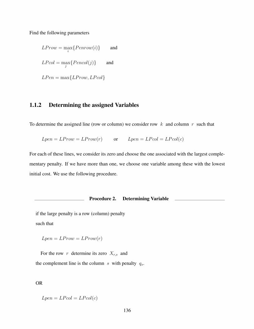
Find the following parameters
LProw = maxi{Penrow(i)} and
LPcol = maxj{Pencol(j)} and
LPen = max{LProw, LPcol}
1.1.2 Determining the assigned Variables
To determine the assigned line (row or column) we consider row k and column r such that
Lpen = LProw = LProw(r) or Lpen = LPcol = LPcol(c)
For each of these lines, we consider its zero and choose the one associated with the largest comple-
mentary penalty. If we have more than one, we choose one variable among these with the lowest
initial cost. We use the following procedure.
Procedure 2. Determining Variable
if the large penalty is a row (column) penalty
such that
Lpen = LProw = LProw(r)
For the row r determine its zero Xr,s and
the complement line is the column s with penalty qs.
OR
Lpen = LPcol = LPcol(c)
136

For the column c determine its zero Xk,c and
the complement line is the row k with penalty pk.
Set UniqueLpen = 1 (Indicate that the Largest Penalty is uniqune )
1.1.3 Null Penalty Case
When all the penalties equal zero then LPen = 0 and there is at least two zeros on each row and
each column.
Proposition 1.1.3.1. When LPen = 0 then the current reduced cost matrix contains a
Zeros independent solution.
This situation include the trivial one where the remaining reduced matrix is null.
Procedure 3. Null Penalty Case
Set MaxZrow = NZrow(1) and row = 1
Set MaxZcol = NZcol(1) and col = 1
While n − NCrossRow ≥ 2 and m − NCrossCol ≥ 2 do
For i = 2, · · · , n do
If crossrow(i) = 0
137

if MaxZrow < NZrow(i) then
MaxZrow = NZrow(i)
row = i
endFor
For j = 2, · · · ,m do
If Crosscol(j) = 0
if MaxZcol < NZcol(j) then
MaxZcol = NZcol(j)
col = j
endFor
Assign Xrow,col
if arow < bcol then
Call procedure 3. Assigning Row
else
if bcol < arow then
Call procedure 4. Assigning Column
else
Call procedure 5. Equality Case
endif
Set crossrow(row) = 1 AND crosscol(col) = 1
Evaluate NCrossRow := NCrossRow + 1 and
NCrossCol := NCrossCol + 1
endWhile
138

1.1.4 Assigning variable
Once the variable is determined, we assign one and cross out the associated row and column.
Procedure 3. Assigning Row
For the variable Xt,z
Set Xt,z = at
Set crossrow(t) = 1
bz = bz − at ( updating the demand)
Zrow(t) = Zrow(t)− {z}
Zcol(z) = Zcol(z)− {t}
NCrossRow = NCrossRow + 1
Procedure 4. Assigning Column
For the variable Xt,z
Set Xt,z = bz
Set crosscol(z) = 1
at = at − bz ( updating the supply)
Zrow(t) = Zrow(t)− {z}
Zcol(z) = Zcol(z)− {t}
NCrossCol = NCrossCol + 1
we consider the situation where pt and qz for the variable Xt,z are equal.
139

Procedure 5. Equality Case
For the variable Xt,z
Set Xt,z = qz = pt
Set crossrow(t) = 1 and crosscol(z) = 1
Zrow(t) = Zrow(t)− {z}
Zcol(z) = Zcol(z)− {t}
NCrossRow = NCrossRow + 1
NCrossCol = NCrossCol + 1
1.1.4.1 Multiple Largest Penalties
Procedure 6. Multiple Penalties
we consider the case when there are multiple largest penalties for rows or columns.
therefore, there are multiple cases have to be considered. refer to section 1.2.
Then we set UniqueLpen = 0
1.1.5 Reduction
1.1.5.1 Null Complementary Column Case
We consider the situation where the column penalty is null and the column c is crossed out.
Note: the column penalties must be re-evaluated.
140
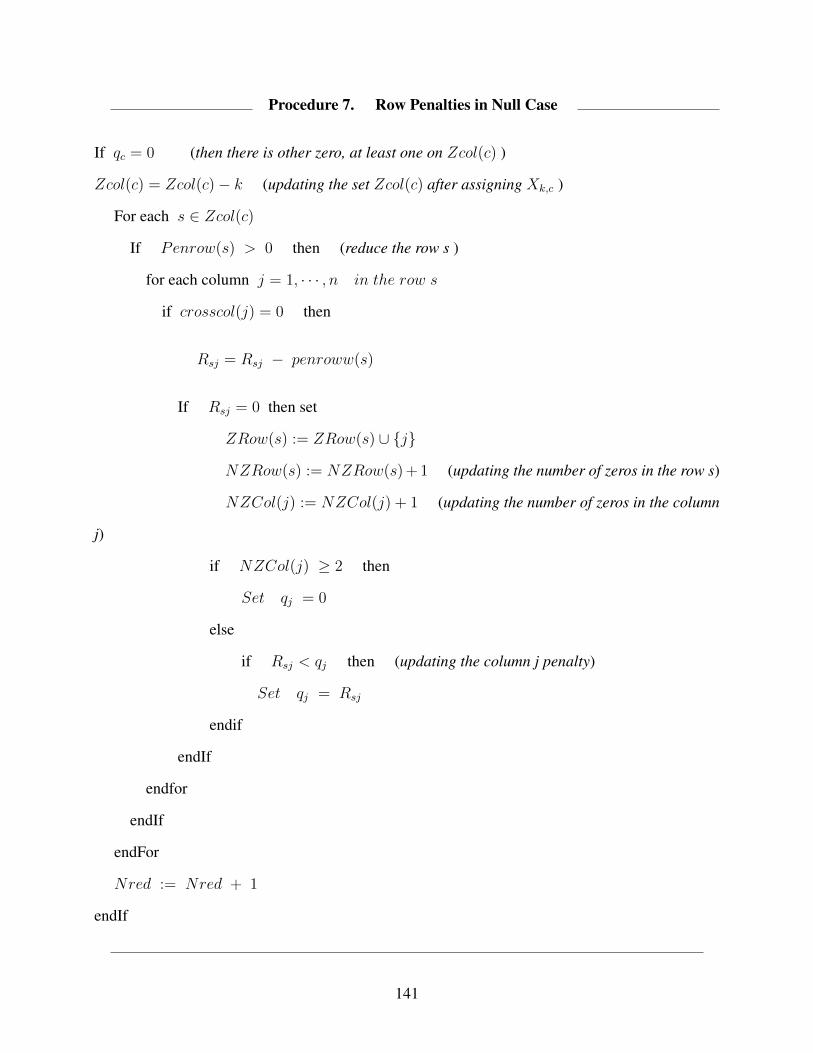
Procedure 7. Row Penalties in Null Case
If qc = 0 (then there is other zero, at least one on Zcol(c) )
Zcol(c) = Zcol(c)− k (updating the set Zcol(c) after assigning Xk,c )
For each s ∈ Zcol(c)
If Penrow(s) > 0 then (reduce the row s )
for each column j = 1, · · · , n in the row s
if crosscol(j) = 0 then
Rsj = Rsj − penroww(s)
If Rsj = 0 then set
ZRow(s) := ZRow(s) ∪ {j}
NZRow(s) := NZRow(s) + 1 (updating the number of zeros in the row s)
NZCol(j) := NZCol(j) + 1 (updating the number of zeros in the column
j)
if NZCol(j) ≥ 2 then
Set qj = 0
else
if Rsj < qj then (updating the column j penalty)
Set qj = Rsj
endif
endIf
endfor
endIf
endFor
Nred := Nred + 1
endIf
141

1.1.5.2 Null Complementary Row Case
We consider the situation where the row penalty is null and the rowr is crossed out.
Note: the row penalties must be re-evaluated.
Procedure 8. Column Penalties in Null Case
If pr = 0 (then there is other zero, at least one on Zrowl(r) )
Zrow(r) = Zrow(r)− {s} (updating the set Zrow(r) after assigning Xr,s )
For each s ∈ Zrow(r)
If Pencol(s) > 0 then (reduce the column s )
for each row i = 1, · · · , n
if crossrow(i) = 0 then
Ris = Ris − pencol(s)
If Ris = 0 then set
ZRow(i) := ZRow(i) ∪ {s}
NZRow(i) := NZRow(i) + 1 (updating the number of zeros in the row i)
NZCol(s) := NZCol(s) + 1 (updating the number of zeros in the column
s)
if NZRow(i) ≥ 2 then
Set pi = 0
else
if Ris < pi then
Set pi = Ris
142

endif
endIf
endfor
endIf
endFor
Nred := Nred + 1
endIf
1.1.6 Updating
1.1.6.1 Row Penalties Evaluation
Procedure 9. Updating Row Penalties
For i = 1, · · · , n do
If crossrow(i) = 0 then
if Ri,z ≤ pi then
if NZRow(i) ≥ 2 then
Set pi = 0
else
Find minj {Ri,j : Ri,j 6= 0}
Set pi = min{Rij : Rij 6= 0}
Endif
endIf
endFor
143

1.1.6.2 Column Penalties Evaluation
Procedure 10. Updating Column Penalties
For j = 1, · · · , n do
If crosscol(j) = 0 then
if Rt,j ≤ qj then
if NZCol(j) ≥ 2 then
Set qj = 0
else
Find mini {Ri,j : Ri,j 6= 0}
Set qj = min{Rij : Rij 6= 0}
Endif
endIf
endFor
1.1.7 General algorithm
Step 1. Cost Matrix Reduction
Call procedure 1. Cost Matrix Reduction
Step 2. Determined the assigned Variables
Call procedure 2. Determining variables
If LPen = 0 then
Call procedure 1. Null penalty
144

print the optimal solution
else
If LPen = LPRow then
if ar < bs then
Call procedure 3. Assigning Row
else
if bs < ar then
Call procedure 4. Assigning Column
else (Equality Case )
Call procedure 5. Equality Case
endif
else
If LPen = LPCol then
if ak < bc then
Call procedure 3. Assigning Row
else
if bc < ak then
Call procedure 4. Assigning Column
else
Call procedure 5. Equality Case
endif
else ( if LPRow = LPCol)
Call procedure 6. Multiple Penalties
endIf
145

Step 3. Stopping Test
If NCrossRow = 1 OR NCrossCol = 1 then
if NCrossRow = 1
For each column j = 1, · · · ,m in row t do
If crosscol(j) = 0 then
Assign Xt,j = bj
endIf
endFor
else ( NCrossCol = 1)
For each row i = 1, · · · , n in column z do
If crossrow(i) = 0 then
Assign Xi,z = ai
endIf
endFor
endif
else
continue
endIf
Step 4. Updating Penalties
If LPen = LPRow then
Call procedure 7. Row Penalties in Null Case
Call procedure 9. Updating Row Penalties
else
If LPen = LPCol then
146
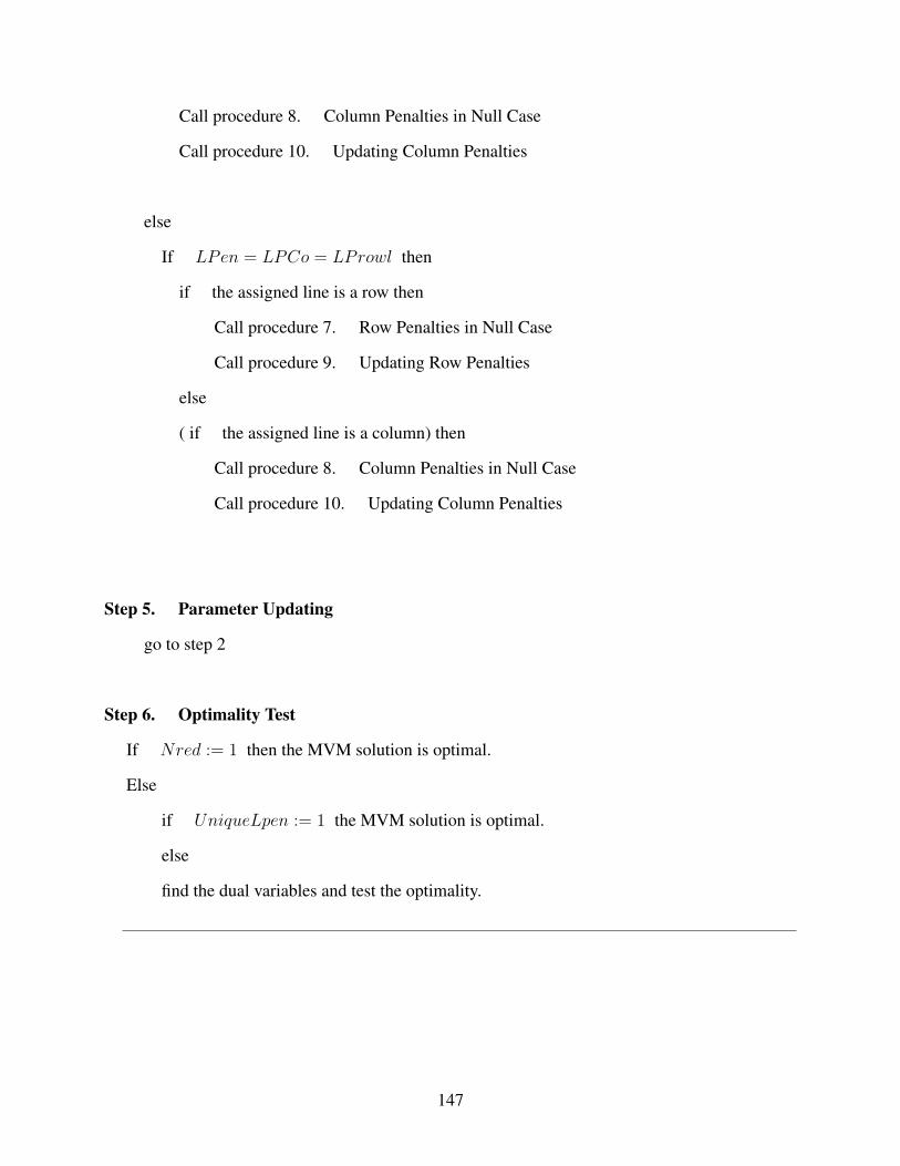
Call procedure 8. Column Penalties in Null Case
Call procedure 10. Updating Column Penalties
else
If LPen = LPCo = LProwl then
if the assigned line is a row then
Call procedure 7. Row Penalties in Null Case
Call procedure 9. Updating Row Penalties
else
( if the assigned line is a column) then
Call procedure 8. Column Penalties in Null Case
Call procedure 10. Updating Column Penalties
Step 5. Parameter Updating
go to step 2
Step 6. Optimality Test
If Nred := 1 then the MVM solution is optimal.
Else
if UniqueLpen := 1 the MVM solution is optimal.
else
find the dual variables and test the optimality.
147

1.2 Special Cases for Multiple Largest Penalties
1.2.1 Largest penalty Row-Column
We consider the situation where there a unique row k and a unique column r such that
LPen = LProw = maxi{Penrow(i)} = Penrow(k) = pk
and
LPen = LPcol = maxj{Penrcol(i)} = Penrow(r) = qr
1.2.1.1 Mutual Complementarity Case
In this case
Rk,r = 0 kc = r and rc = k
There is a unique choice. The variable to be assigned is Xk,r
If ak = br
Assign Xk,r = ak then crossrow(k) =1 (cross out row k)
Find on column r the variable Xrl,r such that Rrl,r = LPen
Set Xrl,r = 0 then crosscol(r) =1 (cross out row r)
else
if ak < br then (Simultaneous assignment, Matrix reduced)
Assign Xk,r = ak then crossrow(k) =1 (cross out column r)
Set br = br − ak then reduce column r
else
if ak > br then
148

Assign Xk,r = br then crosscol(r) =1 (cross out column r)
Set ak = ak − br then reduce row k
endif
endif
endif
1.2.1.2 Confluctual & non-Cnofluctual cases
In this section, we consider the cases when
kc 6= r rc 6= k
Then we have four sub-cases from the supplies and demand perspective :
1.
If ak ≤ bkc and br ≤ arc then
Choose a line with complementary penalty null.
Assign row k if qkc = 0 with Xk,kc = ak
else
Assign column r if prc = 0 with Xr,rc = br
else ( if both complementary lines have non-null penalty)
Compare between ak and br and choose the line with the largest.
cross out out at least a line.
If ak = bkc cross out row k then assign zero to the least cost of column kc
149

and cross out column kc.
If arc = br cross out column r then assign zero to the least cost of row rc
and cross out row rc.
Reduce if necessary the remain matrix.
Endif
2.
If ak ≤ bkc and br > arc then
we are considering two situations when Rk,r > LPen and Rk,r = LPen
case 1: if Rk,r > LPen
Compare the left over costs br − arc and bkc − ak and choose the line with the largest cost.
Then cross out at least a row.
If ak = bkc cross out also column kc after assigning zero to the least cost of that column.
Reduce if necessary the remain matrix.
Endif
case 2: if Rk,r = LPen
The column r has the priority because it will need second lowest cost
Xr,rc = arc
cross out at lest row rc
If ak = bkc cross out row k then assign zero to the least cost of column kc and
cross out column kc.
150

Reduce if necessary the remain matrix.
Update if necessary the row penalties.
Endif
3.
If ak > bkc and br ≤ arc then
we are considering two situations when Rk,r > LPen and Rk,r = LPen
case 1: if Rk,r > LPen
Compare the left over costs arc − ar and ak − bkc and choose the line with the largest cost.
Then cross out at least a column.
If br = arc cross out also row rc after assigning zero to the least cost of that row.
Reduce if necessary the remain matrix.
Endif
case 2: if Rk,r = LPen
The row k has the priority because it will need second lowest cost
Xk,kc = bkc
cross out at least column kc
If br = arc cross out column r then assign zero to the least cost of row rc and
cross out row rc.
Reduce if necessary the remain matrix.
Update if necessary the row penalties.
151
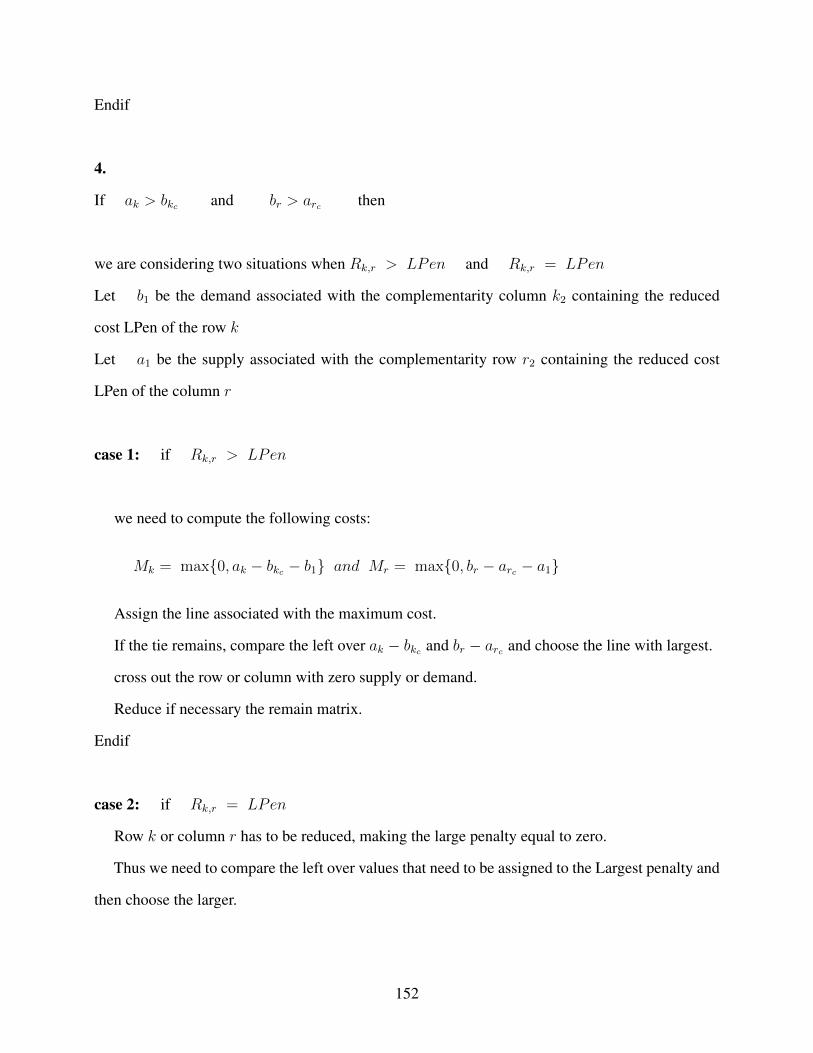
Endif
4.
If ak > bkc and br > arc then
we are considering two situations when Rk,r > LPen and Rk,r = LPen
Let b1 be the demand associated with the complementarity column k2 containing the reduced
cost LPen of the row k
Let a1 be the supply associated with the complementarity row r2 containing the reduced cost
LPen of the column r
case 1: if Rk,r > LPen
we need to compute the following costs:
Mk = max{0, ak − bkc − b1} and Mr = max{0, br − arc − a1}
Assign the line associated with the maximum cost.
If the tie remains, compare the left over ak − bkc and br − arc and choose the line with largest.
cross out the row or column with zero supply or demand.
Reduce if necessary the remain matrix.
Endif
case 2: if Rk,r = LPen
Row k or column r has to be reduced, making the large penalty equal to zero.
Thus we need to compare the left over values that need to be assigned to the Largest penalty and
then choose the larger.
152

By computing the costs:
Mk = max{ak − bkc − br, 0} and Ms = max{br − arc − ak, 0}
Assign the line associated with the maximum cost.
If the tie remains, compare the left over ak − bkc and br − arc and choose the line with largest.
cross out the row or column with zero supply or demand.
Reduce if necessary the remain matrix.
Endif
1.2.2 Largest Penalty Paralleled lines
We consider the situation where there two rows (columns) k and s such that
LPen = LProw = maxi{Penrow(i)} = Penrow(k) = Penrow(s)
The row k contains exactly one zero Rk,kc = 0 which is on the complementary column kc with its
penalty equal to qkc . The supply of the rows k and s are respectively ak and as.
1.2.2.1 Same Complementary Column
In this case, the two rows have the same complementary column:
Rk,kc = 0 Rs,sc = 0 with kc = sc
153

Case 1. ak + as ≤ bkc
Assign Xk,kc = ak and cross out row k .
Set bkc = bkc − ak
then assign Xk,kc = as and cross out row s
If ak + as = bkc then cross out column kc
else
Set bkc = bkc − as
Update the penalties of the rows and column.
Case 2. ak + as > bkc
Let b1 be the demand associated with the complementarity column k2 containing the reduced
cost LPen of the row k
Let b2 be the demand associated with the complementarity column s2 containing the reduced
cost LPen of the row s
Let b = max{b2}
Case 2.1 ak ≤ bkc and as ≤ bkc
First we need to compare the left over with the demands b1 and b2
If ak + as − bkc ≤ b = b2
Assign Xk,kc = ak and cross out row k .
Then assign Xs,kc = bkc − ak and Xs,s2 = ak + as − bkc
cross out row s and column kc
Reduce if necessary the remaining rows that contain their zeros in column kc
154

Update if necessary the row penalties.
If ak + as − bkc ≤ b = b1
Assign Xs,kc = as and cross out row s .
Then assign Xk,kc = bkc − as and Xk,k2 = ak + as − bkc
cross out row k and column kc
Reduce if necessary the remaining rows that contain their zeros in column kc
Update if necessary the row penalties.
If ak + as − bkc > b
Find φk the third largest reduced cost of row k
Find φs the third largest reduced cost of row s
Define the costs:
F (k) = LPen b2 + (ak + as − bkc − b2)φs and
F (s) = LPen b1 + (ak + as − bkc − b1)φk
If F (k) ≤ F (s)
Assign Xk,kc = ak and cross out row k .
Then assign Xs,kc = bkc − ak and Xs,s2 = ak + as − bkc
cross out row s and column kc
Reduce if necessary the remaining rows that contain their zeros in column kc
Update if necessary the row penalties.
else
Assign Xs,kc = as and cross out row s .
Then assign Xk,kc = bkc − as and Xk,k2 = ak + as − bkc
cross out row k and column kc
Reduce if necessary the remaining rows that contain their zeros in column kc
155

Update f necessary the row penalties.
Endif
Case 2.2 ak ≤ bkc and as > bkc
We need to check if there is remaining supplies on row k and s after assigning the largest
penalties.
Define the parameters
Mk = max{0, as + ak − bkc − b2}
Ms = max{0, as − bkc − b2} + max{0, ak − b1}
If Mk > Ms
Assign Xk,kc = ak and cross out row k .
Then assign Xs,kc = bkc − ak and Xs,s2 = min{b2, ak + as − bkc}
cross out column kc and other rows or columns with zero supply or demand
Reduce if necessary the remaining matrix
Update if necessary the penalties.
else
Assign Xs,kc = bkc and cross out column kc .
Then assign Xk,k2 = min{b1, ak} and Xs,s2 = min{b2, as − bkc}
cross out rows or columns with zero supply and demand
Reduce if necessary the remaining matrix
Update f necessary the penalties.
Endif
Case 2.3 ak > bkc and as ≤ bkc
156

We need to check if there is remaining supplies on row k and s after assigning the largest
penalties.
Define the parameters
Mk = max{0, ak − bkc − b1} + max{0, as − b2}
Ms = max{0, ak + as − bkc − b1}
If Mk ≥Ms
Assign Xk,kc = bkc and cross out column kc .
Then assign Xk,k2 = min{b1, ak − bk−c} and Xs,s2 = min{b2, as}
cross out rows or columns with zero supply and demand
Reduce if necessary the remaining matrix
Update f necessary the penalties.
else
Assign Xs,kc = as and cross out row s .
Then assign Xk,kc = bkc − as and Xk,k2 = min{b1, ak + as − bkc}
cross out column kc and other rows or columns with zero supply or demand
Reduce if necessary the remaining matrix
Update if necessary the penalties.
Endif
Case 2.4 ak > bkc and as > bkc
Define the parameters
Mk = max{0, ak − bkc − b1} + max{0, as − b2}
Ms = max{0, as − bkc − b2} + max{0, ak − b1}
If Mk > Ms
157

Assign Xk,kc = bkc and cross out column kc .
Then assign Xk,k2 = min{b1, ak − bk−c} and Xs,s2 = min{b2, as}
cross out rows or columns with zero supply and demand
Reduce if necessary the remaining matrix
Update f necessary the penalties.
else
Assign Xs,kc = bkc and cross out column kc .
Then assign Xk,k2 = min{b1, ak} and Xs,s2 = min{b2, as − bkc}
cross out rows or columns with zero supply and demand
Reduce if necessary the remaining matrix
Update f necessary the penalties.
Endif
1.2.2.2 Different Complementary Columns
In this case, the two rows or columns have different complementary columns.Since analysis for two
columns are similar, we consider the situation two rows
Rk,kc = 0 Rs,sc = 0 with kc 6= sc
Case 1. If ak ≤ bkc and as ≤ bsc then
Assign simultaneously Xk,kc = ak Xs,kc = as
Cross out at least two rows k and s
If ak = bkc assign zero to the least cost of column kc and Cross out column kc
If as = bsc assign zero to the least cost of column sc and Cross out column sc
else
158

Set bkc = bkc − ak and bsc = bsc − as
Then we reduce if necessary the columns kc and sc .
Update the penalties of the rows and columns.
Case 2. If ak ≤ bkc and as > bsc then
Row s has the priority to avoid having the reduction for row s and to have less left-over quantity
on the demand.
Xs,kc = bsc
Cross out column sc
Set as = as − bsc
Then we reduce row s .
Update the penalties of the rows and columns.
Case 3. If ak > bkc and as ≤ bsc then
Row k has the priority to avoid having the reduction for row k and to have less left-over quntity
on the demand.
Xk,kc = bkc
Cross out column kc
Set ak = ak − bkc
Then we reduce row k .
Update the penalties of the rows and columns.
Case 4. If ak > bkc and as > bsc then
159

we are considering four situations as following:
If Rk,sc = LPen and Rs,kc > LPen
Assign Xk,kc = bkc and cross out the column kc
Set ak = ak − bkc
Then we reduce if necessary the rows.
Evaluate the penalties of the rows and columns.
If Rk,sc > LPen and Rs,kc = LPen
Assign Xs,kc = bsc and cross out the column sc
Set as = as − bsc
Then we reduce if necessary the rows.
Evaluate the penalties of the rows and column.
If Rk,sc = LPen and Rs,kc = LPen
Both rows k and s will need at least their second least costs and may need the third lest costs.
So, we need to compare the left over quantities for rows k and s
Define the parameters
Mk = max{0, ak − bkc − bsc}
Ms = max{0, as − bsc − bkc}
If Mk > Ms
Assign Xk,kc = bkc and cross out column kc .
cross out rows or columns with zero supply and demand
Reduce if necessary the remaining matrix
160

Update f necessary the penalties.
else
if Ms > Mk
Assign Xs,kc = bkc and cross out column kc .
cross out rows or columns with zero supply and demand
Reduce if necessary the remaining matrix
Update f necessary the penalties.
else
comparison between (ak−bkc) and (as−bsc) and assign line associates with the larger
Endif
If Rk,sc > LPen and Rs,kc > LPen
Let b1 be the demand associated with the complementarity column k2 containing the reduced
cost LPen of the row k
Let b2 be the demand associated with the complementarity column s2 containing the reduced
cost LPen of the row s
Define the parameters
Mk = max{0, ak − bkc − b1}
Ms = max{0, as − bsc − b2}
If Mk > Ms
Assign Xk,kc = bkc and cross out column kc .
cross out rows or columns with zero supply and demand
Reduce if necessary the remaining matrix
Update f necessary the penalties.
161

else
if Ms > Mk
Assign Xs,kc = bkc and cross out column kc .
cross out rows or columns with zero supply and demand
Reduce if necessary the remaining matrix
Update f necessary the penalties.
else
comparison between (ak − bkc) and (as − bsc) and assign the line associates with the
larger
162
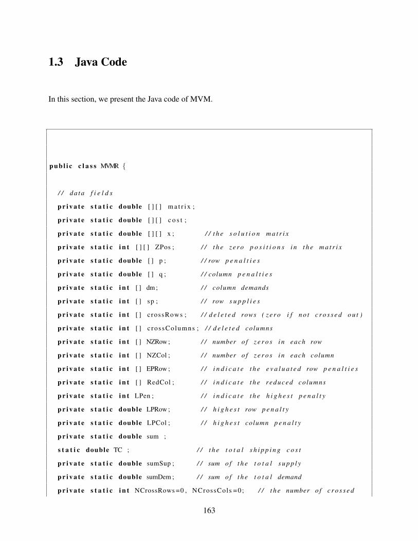
1.3 Java Code
In this section, we present the Java code of MVM.
p u b l i c c l a s s MVMR {
/ / da ta f i e l d s
p r i v a t e s t a t i c double [ ] [ ] m a t r i x ;
p r i v a t e s t a t i c double [ ] [ ] c o s t ;
p r i v a t e s t a t i c double [ ] [ ] x ; / / t h e s o l u t i o n m a t r i x
p r i v a t e s t a t i c i n t [ ] [ ] ZPos ; / / t h e z e r o p o s i t i o n s i n t h e m a t r i x
p r i v a t e s t a t i c double [ ] p ; / / row p e n a l t i e s
p r i v a t e s t a t i c double [ ] q ; / / column p e n a l t i e s
p r i v a t e s t a t i c i n t [ ] dm ; / / column demands
p r i v a t e s t a t i c i n t [ ] sp ; / / row s u p p l i e s
p r i v a t e s t a t i c i n t [ ] crossRows ; / / d e l e t e d rows ( z e r o i f n o t c r o s s e d o u t )
p r i v a t e s t a t i c i n t [ ] c rossColumns ; / / d e l e t e d columns
p r i v a t e s t a t i c i n t [ ] NZRow; / / number o f z e r o s i n each row
p r i v a t e s t a t i c i n t [ ] NZCol ; / / number o f z e r o s i n each column
p r i v a t e s t a t i c i n t [ ] EPRow ; / / i n d i c a t e t h e e v a l u a t e d row p e n a l t i e s
p r i v a t e s t a t i c i n t [ ] RedCol ; / / i n d i c a t e t h e reduced columns
p r i v a t e s t a t i c i n t LPen ; / / i n d i c a t e t h e h i g h e s t p e n a l t y
p r i v a t e s t a t i c double LPRow ; / / h i g h e s t row p e n a l t y
p r i v a t e s t a t i c double LPCol ; / / h i g h e s t column p e n a l t y
p r i v a t e s t a t i c double sum ;
s t a t i c double TC ; / / t h e t o t a l s h i p p i n g c o s t
p r i v a t e s t a t i c double sumSup ; / / sum o f t h e t o t a l s u p p l y
p r i v a t e s t a t i c double sumDem ; / / sum o f t h e t o t a l demand
p r i v a t e s t a t i c i n t NCrossRows =0 , NCrossCols =0; / / t h e number o f c r o s s e d
163
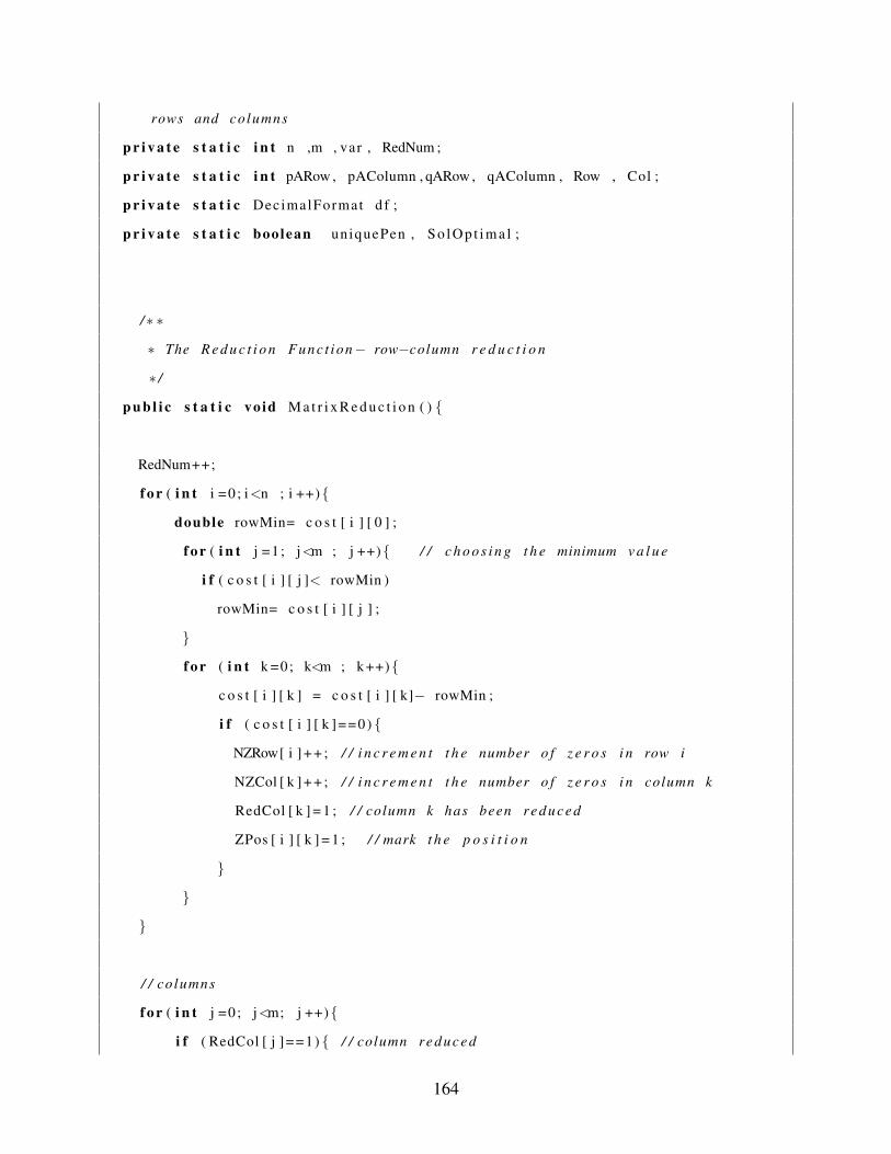
rows and columns
p r i v a t e s t a t i c i n t n ,m , var , RedNum ;
p r i v a t e s t a t i c i n t pARow , pAColumn , qARow , qAColumn , Row , Col ;
p r i v a t e s t a t i c DecimalFormat d f ;
p r i v a t e s t a t i c boolean uniquePen , S o l O p t i m a l ;
/∗ ∗
∗ The R e d u c t i o n Func t ion− row−column r e d u c t i o n
∗ /
p u b l i c s t a t i c vo id M a t r i x R e d u c t i o n ( ) {
RedNum++;
f o r ( i n t i =0 ; i<n ; i ++){
double rowMin= c o s t [ i ] [ 0 ] ;
f o r ( i n t j =1 ; j<m ; j ++){ / / c h o o s i n g t h e minimum v a l u e
i f ( c o s t [ i ] [ j ]< rowMin )
rowMin= c o s t [ i ] [ j ] ;
}
f o r ( i n t k =0; k<m ; k ++){
c o s t [ i ] [ k ] = c o s t [ i ] [ k]− rowMin ;
i f ( c o s t [ i ] [ k ]==0) {
NZRow[ i ] + + ; / / i n c r e m e n t t h e number o f z e r o s i n row i
NZCol [ k ] + + ; / / i n c r e m e n t t h e number o f z e r o s i n column k
RedCol [ k ] = 1 ; / / column k has been reduced
ZPos [ i ] [ k ] = 1 ; / / mark t h e p o s i t i o n
}
}
}
/ / co lumns
f o r ( i n t j =0 ; j<m; j ++){
i f ( RedCol [ j ]==1) { / / column reduced
164

i f ( NZCol [ j ] >=2){ / / i f t h e r e are more than one z e r o
q [ j ] = 0 ;
}
e l s e { / / i f t h e r e i s o n l y one z e r o
double colMin= sum ;
/ / c h o o s i n g t h e minimum v a l u e
f o r ( i n t i =0 ; i<n ; i ++){ / / i =0
i f ( c o s t [ i ] [ j ]< colMin && c o s t [ i ] [ j ] ! = 0 )
colMin= c o s t [ i ] [ j ] ;
}
q [ j ]= colMin ;
}
}
e l s e { / / i f t h e column i s n o t reduced y e t
double colMin= c o s t [ 0 ] [ j ] ;
/ / c h o o s i n g t h e minimum v a l u e
f o r ( i n t i =1 ; i<n ; i ++){ / / i =0
i f ( c o s t [ i ] [ j ]< colMin )
colMin= c o s t [ i ] [ j ] ;
}
double [ ] m i n L i s t = new double [ n ] ;
f o r ( i n t k =0; k<n ; k ++){
c o s t [ k ] [ j ] −= colMin ;
m i n L i s t [ k ]= c o s t [ k ] [ j ] ; / / t o compute t h e column p e n a l t y
i f ( c o s t [ k ] [ j ]==0) {
NZRow[ k ] + + ;
NZCol [ j ] + + ; / / i n c r e m e n t t h e number o f z e r o s i n column k
p [ k ] = 0 ; / / re−compute t h e row p e n a l t y
EPRow[ k ] = 1 ; / / mark t h e e v a l u a t e d p e n a l t y
ZPos [ k ] [ j ] = 1 ;
}
}
165

A rr ay s . s o r t ( m i n L i s t ) ;
q [ j ]= m i n L i s t [1]−m i n L i s t [ 0 ] ; / / column p e n a l t i e s
} / / end e l s e
} / / e n d f o r
/ / choose t h e row p e n a l t i e s
f o r ( i n t i =0 ; i<n ; i ++){
i f ( EPRow[ i ] ! = 1 ) { / / i f t h e row p e n a l t y n o t e v a l u a t e d
i f (NZRow[ i ] >=2){
p [ i ] = 0 ;
}
e l s e {
/ / o t h e r w i s e , i f t h e p e n a l t i e s v a l u e s o t h e r than z e r o s
double rowMin= sum ;
/ / c h o o s i n g t h e minimum v a l u e
f o r ( i n t j =0 ; j<m ; j ++){ / / i =0
i f ( c o s t [ i ] [ j ]< rowMin && c o s t [ i ] [ j ] ! = 0 )
rowMin= c o s t [ i ] [ j ] ;
}
p [ i ]= rowMin ;
} / / end e l s e
} / / end i f
} / / end f o r
}
/∗ ∗
∗ T h i s f u n c t i o n d e t e r m i n e s t h e a s s i g n i n g v a r i a b l e s
∗ /
p u b l i c s t a t i c vo id C o n s i d e r i n g V a r i a b l e ( ) {
LPRow=−1;
pARow=−1;
LPCol= −1;
166

qAColumn= −1;
LPen=−1;
f o r ( i n t i =0 ; i<n ; i ++){
i f ( crossRows [ i ] !=1 ) {
i f ( i ==0){
LPRow=p [ 0 ] ;
pARow=0;
f o r ( i n t j =0 ; j<m ; j ++){ / / choose t h e minimum
i f ( ( c rossColumns [ j ] ! = 1 ) && ZPos [ 0 ] [ j ]==1) {
pAColumn= j ; / / column
}
}
}
e l s e i f ( p [ i ]> LPRow) {
LPRow=p [ i ] ;
pARow= i ;
f o r ( i n t j =0 ; j<m ; j ++){ / / choose t h e minimum
i f ( ( c rossColumns [ j ] ! = 1 ) && ZPos [pARow ] [ j ]==1) {
pAColumn= j ;
}
}
}
e l s e i f ( p [ i ] == LPRow) { / / p a r a l l e l rows
i n t pos2 =0;
f o r ( i n t j =0 ; j<m ; j ++){ / / choose t h e minimum
i f ( ( c rossColumns [ j ] ! = 1 ) && ZPos [ i ] [ j ]==1) {
pos2= j ;
}
}
/ / i f t h e complementary columns are t h e same
i f ( pos2 == pAColumn && m−NCrossCols ! = 2 ) {
/ / 2 c a s e s
167

/ / i f ( sp [ i ] +sp [pARow] <= dm[ pAColumn ] ) {
/ / s i m u l t a n e o u s l y
i f ( sp [ i ] +sp [pARow] > dm[ pAColumn ] ) { / / 4 s u b c a s e s
i n t b1=−1 , b2=−1, max=−1;
A r r a y L i s t<Double> min1= new A r r a y L i s t<Double >() ;
A r r a y L i s t<Double> min2 = new A r r a y L i s t<Double >() ;
double ph i1 =0 , ph i2 =0 , fpARow , f i ;
f o r ( i n t c =0; c<m; c ++){
i f ( c rossColumns [ c ] ! = 1 ) {
min1 . add ( c o s t [pARow ] [ c ] ) ;
min2 . add ( c o s t [ i ] [ c ] ) ;
i f ( c o s t [pARow ] [ c ]== LPRow)
b1=c ;
i f ( c o s t [ i ] [ c ]== LPRow)
b2=c ;
}
} / / end f o r
C o l l e c t i o n s . s o r t ( min1 ) ;
C o l l e c t i o n s . s o r t ( min2 ) ;
ph i1 = min1 . g e t ( 2 ) ; / / phi−k
ph i2 = min2 . g e t ( 2 ) ; / / phi−s
i f (dm[ b1 ] >= dm[ b2 ] )
max =0; / / b1
e l s e
max =1; / / b2
i f ( sp [pARow] <= dm[ pAColumn ] && sp [ i ] <= dm[ pAColumn ] ) { / / 1
i f ( max==0 && ( sp [pARow]+ sp [ i ]−dm[ pAColumn ] ) <= dm[ b1 ] ) {
pARow= i ;
168

}
e l s e i f ( ( sp [pARow]+ sp [ i ]−dm[ pAColumn ] ) > dm[ b1 ] | | ( sp [pARow
]+ sp [ i ]−dm[ pAColumn ] )> dm[ b2 ] ) {
/ / need t h e 3 rd
fpARow= (LPRow∗dm[ b2 ] ) + ( ( sp [pARow]+ sp [ i ]−dm[ pAColumn]−
dm[ b2 ] ) ∗ ph i2 ) ;
f i = (LPRow∗dm[ b1 ] ) + ( ( sp [pARow]+ sp [ i ]−dm[ pAColumn]−dm[
b1 ] ) ∗ ph i1 ) ;
i f ( fpARow > f i )
pARow= i ;
/ / e l s e rema ins
}
}
e l s e i f ( sp [pARow] <= dm[ pAColumn ] && sp [ i ] > dm[ pAColumn ] ) { / /
2
fpARow = Math . max ( 0 , ( sp [ i ]− dm[ pAColumn ] + sp [pARow] −dm[ b2
] ) ) ;
f i = Math . max ( 0 , ( sp [ i ]− dm[ pAColumn ] −dm[ b2 ] ) ) +
Math . max ( 0 , ( sp [pARow]− dm[ b1 ] ) ) ;
/ / i f ( fRow > sRow )
/ / pARow=pARow ;
i f ( f i >= fpARow )
pARow= i ; / / s
}
e l s e i f ( sp [pARow] > dm[ pAColumn ] && sp [ i ] <= dm[ pAColumn ] ) { / /
3
fpARow = Math . max ( 0 , ( sp [pARow]− dm[ pAColumn ] −dm[ b1 ] ) ) +
169

Math . max ( 0 , ( sp [ i ]− dm[ b2 ] ) ) ;
f i = Math . max ( 0 , ( sp [pARow]− dm[ pAColumn ] + sp [ i ] −dm[ b1 ] ) )
;
/ / i f ( fRow >= sRow )
/ / pARow=pARow ;
i f ( f i > fpARow )
pARow= i ;
}
e l s e i f ( sp [pARow] > dm[ pAColumn ] && sp [ i ] > dm[ pAColumn ] ) { / / 4
fpARow = Math . max ( 0 , ( sp [pARow]− dm[ pAColumn ] −dm[ b1 ] ) ) +
Math . max ( 0 , ( sp [ i ]− dm[ b2 ] ) ) ;
f i = Math . max ( 0 , ( sp [ i ]− dm[ pAColumn ] −dm[ b2 ] ) ) +
Math . max ( 0 , ( sp [pARow]− dm[ b1 ] ) ) ;
/ / i f ( fRow >= sRow )
/ / pARow=pARow ;
i f ( f i > fpARow )
pARow= i ;
}
} / / e l s e end
}
e l s e { / / d i f f e r e n t complementary column
/ / 4 c a s e s
i f ( sp [pARow] <= dm[ pAColumn ] && sp [ i ] <= dm[ pos2 ] ) {
i f ( ( dm[ pos2 ] − sp [ i ] ) > (dm[ pAColumn ] − sp [pARow ] ) ) {
pARow= i ;
170

pAColumn=pos2 ;
}
/ / e l s e− t h e same
}
e l s e i f ( sp [pARow] <= dm[ pAColumn ] && sp [ i ] > dm[ pos2 ] ) {
pARow= i ;
pAColumn=pos2 ;
}
/ / i f ( sp [pARow] > dm[ pAColumn ] && sp [ i ] <= dm[ pos2 ] )
/ / t h e same pARow
e l s e i f ( sp [pARow] > dm[ pAColumn ] && sp [ i ] > dm[ pos2 ] ) {
/ / 4 c a s e s
/ / i f ( c o s t [pARow ] [ pos2]== LPRow && c o s t [ i ] [ pAColumn ]!= LPRow )
/ / LPRow remains
i f ( c o s t [pARow ] [ pos2 ] ! = LPRow && c o s t [ i ] [ pAColumn]== LPRow) {
pARow= i ;
pAColumn=pos2 ;
}
e l s e {
/ / compare t h e l e f t ove r
i f (m−NCrossCols ==2){
/ / i f ( ( sp [pARow]−dm[ pAColumn ] ) > ( sp [ i ] − dm[ pos2 ] ) )
/ / LPRow remains
i f ( ( sp [pARow]−dm[ pAColumn ] ) < ( sp [ i ] − dm[ pos2 ] ) ) {
pARow= i ;
pAColumn=pos2 ;
}
}
e l s e { / / i f (m−NCrossCols !=2)
171

i f ( c o s t [ i ] [ pAColumn]== LPRow && c o s t [pARow ] [ pos2 ]== LPRow
) {
double fRow = Math . max ( 0 , ( sp [pARow] − dm[ pAColumn ] −
dm[ pos2 ] ) ) ;
double sRow = Math . max ( 0 , ( sp [ i ] − dm[ pos2 ] − dm[
pAColumn ] ) ) ;
/ / i f ( fRow > sRow )
/ / pARow t h e same
i f ( sRow > fRow ) {
pARow= i ;
pAColumn=pos2 ;
}
e l s e i f ( sRow == fRow ) {
i f ( ( sp [ i ] − dm[ pos2 ] ) > ( sp [pARow] − dm[ pAColumn ] ) )
{
pARow= i ;
pAColumn=pos2 ;
}
}
}
e l s e i f ( c o s t [pARow ] [ pos2 ] ! = LPRow && c o s t [ i ] [ pAColumn ] ! =
LPRow) {
i n t b1=−1, b2=−1;
f o r ( i n t c =0; c<m; c ++){
i f ( c rossColumns [ c ] ! = 1 ) {
i f ( c o s t [pARow ] [ c ]== LPRow)
b1=c ; / / f i r s t row
i f ( c o s t [ i ] [ c ]== LPRow)
172

b2=c ; / / s econd row
}
} / / end f o r
double fRow = Math . max ( 0 , ( sp [pARow] − dm[ pAColumn ] −
dm[ b1 ] ) ) ;
double sRow = Math . max ( 0 , ( sp [ i ] − dm[ pos2 ] − dm[ b2 ] ) )
;
/ / i f ( fRow > sRow )
/ / pARow t h e same
i f ( sRow > fRow ) {
pARow= i ;
pAColumn=pos2 ;
}
e l s e i f ( sRow == fRow ) {
i f ( ( sp [ i ] − dm[ pos2 ] ) > ( sp [pARow] − dm[ pAColumn ] ) )
{
pARow= i ;
pAColumn=pos2 ;
}
}
}
} / / i f end
}
}
} / / e n d i f
} / / end i f
}
} / / end f o r
/ / e v a l u a t e t h e l a r g e s t p e n a l t y
173

f o r ( i n t j =0 ; j <m; j ++){
i f ( c rossColumns [ j ] ! = 1 ) {
i f ( j ==0){
LPCol= q [ 0 ] ;
qAColumn= 0 ; / / column
f o r ( i n t i =0 ; i<n ; i ++){ / / choose t h e minimum
i f ( ( crossRows [ i ] ! = 1 ) && ZPos [ i ] [ 0 ] = = 1 ) {
qARow= i ; / / row
}
}
}
e l s e i f ( q [ j ]> LPCol ) {
LPCol= q [ j ] ;
qAColumn= j ;
f o r ( i n t i =0 ; i<n ; i ++){ / / choose t h e minimum
i f ( ( crossRows [ i ] ! = 1 ) && ZPos [ i ] [ qAColumn ]==1) {
qARow= i ;
}
}
}
e l s e i f ( q [ j ]== LPCol ) { / / p a r a l l e l e q u a l i t y
i n t pos3 =0;
f o r ( i n t i =0 ; i<n ; i ++){ / / choose t h e minimum
i f ( ( crossRows [ i ] ! = 1 ) && ZPos [ i ] [ j ]==1) {
pos3= i ;
}
}
/ / i f t h e columns have t h e same complementary row
i f ( pos3 == qARow && n−NCrossRows ! = 2 ) {
/ / 2 c a s e s
/ / i f ( dm[ qAColumn]+dm[ j ] <= sp [qARow ] )
/ / a s s i g n s i m u l t a n e o u s l y
174
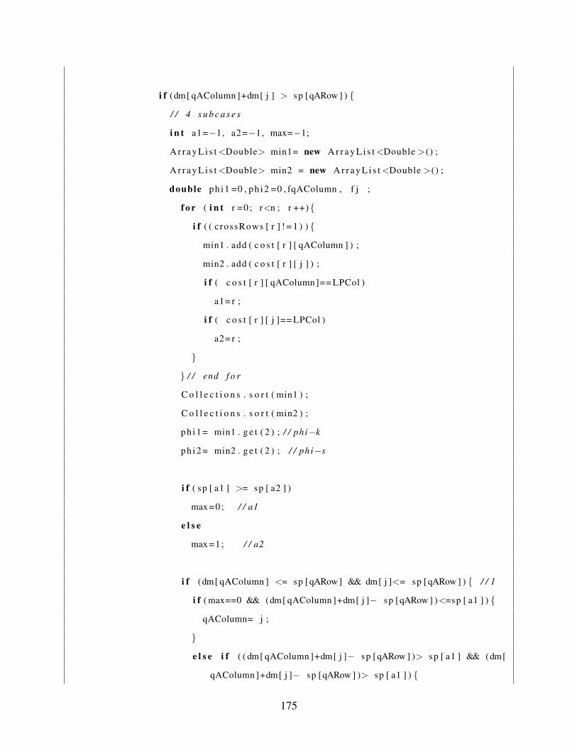
i f (dm[ qAColumn ]+dm[ j ] > sp [qARow ] ) {
/ / 4 s u b c a s e s
i n t a1 =−1, a2 =−1, max=−1;
A r r a y L i s t<Double> min1= new A r r a y L i s t<Double >() ;
A r r a y L i s t<Double> min2 = new A r r a y L i s t<Double >() ;
double ph i1 =0 , ph i2 =0 , fqAColumn , f j ;
f o r ( i n t r =0 ; r<n ; r ++){
i f ( ( crossRows [ r ] ! = 1 ) ) {
min1 . add ( c o s t [ r ] [ qAColumn ] ) ;
min2 . add ( c o s t [ r ] [ j ] ) ;
i f ( c o s t [ r ] [ qAColumn]== LPCol )
a1= r ;
i f ( c o s t [ r ] [ j ]== LPCol )
a2= r ;
}
} / / end f o r
C o l l e c t i o n s . s o r t ( min1 ) ;
C o l l e c t i o n s . s o r t ( min2 ) ;
ph i1 = min1 . g e t ( 2 ) ; / / phi−k
ph i2 = min2 . g e t ( 2 ) ; / / phi−s
i f ( sp [ a1 ] >= sp [ a2 ] )
max =0; / / a1
e l s e
max =1; / / a2
i f (dm[ qAColumn ] <= sp [qARow] && dm[ j ]<= sp [qARow ] ) { / / 1
i f ( max==0 && (dm[ qAColumn ]+dm[ j ]− sp [qARow ] )<=sp [ a1 ] ) {
qAColumn= j ;
}
e l s e i f ( ( dm[ qAColumn ]+dm[ j ]− sp [qARow ] )> sp [ a1 ] && (dm[
qAColumn ]+dm[ j ]− sp [qARow ] )> sp [ a1 ] ) {
175

/ / need t h e 3 rd
fqAColumn= ( sp [ a2 ]∗ LPCol ) + ( ( dm[ qAColumn ]+dm[ j ]− sp [
qARow]− sp [ a2 ] ) ∗ ph i2 ) ;
f j =( sp [ a1 ]∗ LPCol ) + ( ( dm[ qAColumn ]+dm[ j ]− sp [qARow]− sp
[ a1 ] ) ∗ ph i1 ) ;
i f ( fqAColumn> f j )
qAColumn= j ;
}
}
e l s e i f (dm[ qAColumn ] <= sp [qARow] && dm[ j ] > sp [qARow ] ) {
/ / 2
fqAColumn = Math . max ( 0 , (dm[ j ]− sp [qARow] + dm[
qAColumn ] − sp [ a2 ] ) ) ;
f j = Math . max ( 0 , (dm[ j ]− sp [qARow] − sp [ a2 ] ) ) +
Math . max ( 0 , (dm[ qAColumn]− sp [ a1 ] ) ) ;
/ / i f ( f C o l > sCol )
/ / qAColumn= qAColumn ;
i f ( f j >= fqAColumn )
qAColumn= j ; / / s c
}
e l s e i f (dm[ qAColumn ] > sp [qARow] && dm[ j ]<= sp [qARow ] ) { / /
3
fqAColumn = Math . max ( 0 , (dm[ qAColumn]− sp [qARow] − sp [ a1
] ) ) +
Math . max ( 0 , (dm[ j ]− sp [ a2 ] ) ) ;
f j = Math . max ( 0 , (dm[ qAColumn]− sp [qARow] + dm[ j ] − sp [ a1
176

] ) ) ;
/ / i f ( f C o l >= sCol )
/ / qAColumn = qAColumn ;
i f ( f j > fqAColumn )
qAColumn= j ;
}
e l s e i f (dm[ qAColumn ] > sp [qARow] && dm[ j ]> sp [qARow] ) { / / 4
fqAColumn = Math . max ( 0 , (dm[ qAColumn]− sp [qARow] − sp [ a1 ] )
) +
Math . max ( 0 , (dm[ j ]− sp [ a2 ] ) ) ;
f j = Math . max ( 0 , (dm[ j ]− sp [qARow] − sp [ a2 ] ) ) +
Math . max ( 0 , (dm[ qAColumn]− sp [ a1 ] ) ) ;
/ / i f ( f C o l >= sCol )
/ / qAColumn = qAColumn ;
i f ( f j > fqAColumn )
qAColumn= j ;
}
}
}
e l s e { / / d i f f e r e n t complementary row
/ / 4 c a s e s / /
i f (dm[ qAColumn ] <= sp [qARow] && dm[ j ] <= sp [ pos3 ] ) {
/ / both− b u t here
i f ( ( sp [ pos3 ] − dm[ j ] ) > ( sp [qARow] − dm[ qAColumn ] ) ) {
177

qAColumn= j ;
qARow=pos3 ;
}
/ / e l s e− t h e same
}
/ / i f ( dm[ qAColumn ] > sp [qARow] && dm[ j ] <= sp [ pos3 ] )
/ / t h e same qAColumn
e l s e i f (dm[ qAColumn ] <= sp [qARow] && dm[ j ] > sp [ pos3 ] ) {
qAColumn= j ;
qARow=pos3 ;
}
e l s e i f ( dm[ qAColumn ] > sp [qARow] && dm[ j ] > sp [ pos3 ] ) {
/ / 4 c a s e s
/ / i f ( c o s t [ pos3 ] [ qAColumn ] == LPCol && c o s t [qARow ] [ j ] !=
LPCol )
/ / LPCol rema ins
i f ( c o s t [ pos3 ] [ qAColumn ] != LPCol && c o s t [qARow ] [ j ] == LPCol )
{
qAColumn= j ;
qARow=pos3 ;
}
e l s e {
/ / compare t h e l e f t ove r
i f ( n−NCrossRows ==2){
/ / i f ( ( dm[ qAColumn]−sp [qARow ] ) > ( dm[ j ] − sp [ pos3 ] ) )
/ / LPCol rema ins
i f ( ( dm[ qAColumn]− sp [qARow ] ) < (dm[ j ] − sp [ pos3 ] ) ) {
qAColumn= j ;
178

qARow=pos3 ;
}
}
e l s e { / / n−NCrossRows !=2
i f ( c o s t [qARow ] [ j ] == LPCol && c o s t [ pos3 ] [ qAColumn ] ==
LPCol ) {
double fCo l = Math . max ( 0 , (dm[ qAColumn]− sp [qARow] −
sp [ pos3 ] ) ) ;
double sCol = Math . max ( 0 , (dm[ j ] − sp [ pos3 ] − sp [qARow
] ) ) ;
/ / i f ( f C o l > sCol )
/ / t h e same
i f ( sCol > fCo l ) {
qAColumn= j ;
qARow=pos3 ;
}
e l s e i f ( sCol == fCo l ) {
i f ( ( dm[ j ] − sp [ pos3 ] ) > (dm[ qAColumn]− sp [qARow ] )
) {
qAColumn= j ;
qARow=pos3 ;
}
}
}
e l s e i f ( c o s t [qARow ] [ j ] != LPCol && c o s t [ pos3 ] [ qAColumn ]
!= LPCol ) {
i n t a1= −1, a2= −1 ;
f o r ( i n t r =0 ; r<n ; r ++){
i f ( ( crossRows [ r ] ! = 1 ) ) {
179

i f ( c o s t [ r ] [ qAColumn]== LPCol )
a1= r ; / / f
i f ( c o s t [ r ] [ j ]== LPCol )
a2= r ; / / s
}
} / / end f o r
double fCo l = Math . max ( 0 , (dm[ qAColumn]− sp [qARow] −
sp [ a1 ] ) ) ;
double sCol = Math . max ( 0 , (dm[ j ] − sp [ pos3 ] − sp [
qARow ] ) ) ;
/ / i f ( f C o l > sCol )
/ / t h e same
i f ( sCol > fCo l ) {
qAColumn= j ;
qARow=pos3 ;
}
e l s e i f ( sCol == fCo l ) {
i f ( ( dm[ j ] − sp [ pos3 ] ) > (dm[ qAColumn]− sp [qARow ] )
) {
qAColumn= j ;
qARow=pos3 ;
}
}
}
} / / i f end
}
}
} / / e l s e end
} / / end i f
} / / end i f
} / / end f o r
180

/ / e v a l u a t e t h e l a r g e s t p e n a l t y
i f (LPRow > LPCol )
LPen= 0 ; / / LPRow
e l s e i f ( LPCol > LPRow)
LPen= 1 ; / / LPCol
e l s e { / / non= p a r a l l e l e q u a l i t y
/ / 3 c a s e s
i f (pARow == qARow && qAColumn == pAColumn ) / / mu tua l
LPen= 0 ; / / LPRow ;
e l s e {
/ / non−c o n f l i c t e d
i f ( sp [pARow] <= dm[ pAColumn ] && dm[ qAColumn]<= sp [qARow ] ) {
i f ( q [ pAColumn ] ==0)
LPen= 0 ;
e l s e i f ( p [qARow]==0)
LPen= 1 ;
e l s e {
i f ( sp [pARow] >= dm[ qAColumn ] )
LPen= 0 ;
e l s e
LPen= 1 ;
}
}
e l s e i f ( sp [pARow] <= dm[ pAColumn ] && dm[ qAColumn]> sp [qARow ] ) {
i f ( c o s t [pARow ] [ qAColumn ] == LPCol )
LPen= 1 ;
e l s e {
181

i f ( ( dm[ pAColumn ] − sp [pARow ] ) > (dm[ qAColumn ] − sp [qARow ] ) )
LPen= 0 ;
e l s e
LPen= 1 ;
}
}
e l s e i f ( sp [pARow] > dm[ pAColumn ] && dm[ qAColumn]<= sp [qARow ] ) {
i f ( c o s t [pARow ] [ qAColumn ] == LPCol )
LPen= 0 ;
e l s e {
i f ( ( sp [pARow] − dm[ pAColumn ] )> ( sp [qARow] −dm[ qAColumn ] ) )
LPen= 1 ;
e l s e
LPen= 0 ;
}
}
e l s e {
i f ( c o s t [pARow ] [ qAColumn ] == LPCol ) {
i f ( n−NCrossRows !=2 && m−NCrossCols ! = 2 ) {
double row2 = sp [pARow] − dm[ pAColumn ] ;
double c o l 2 = dm[ qAColumn ] − sp [qARow ] ;
double row = Math . max ( 0 , sp [pARow]− dm[ pAColumn]− dm[
qAColumn ] ) ;
double c o l = Math . max ( 0 , dm[ qAColumn]− sp [qARow] − sp [
pARow ] ) ;
i f ( row > c o l )
LPen= 0 ;
e l s e i f ( row < c o l )
LPen= 1 ;
182

e l s e {
i f ( row2 > c o l 2 )
LPen= 0 ;
e l s e
LPen= 1 ;
}
}
e l s e {
i f ( n−NCrossRows ==2)
LPen= 1 ;
e l s e
LPen =0;
}
}
e l s e { / / != LPCol
/ / bo th
i n t b= −1 , a = −1 ;
f o r ( i n t r =0 ; r<n ; r ++){
i f ( ( crossRows [ r ] ! = 1 ) && c o s t [ r ] [ qAColumn]== LPCol )
a= r ;
}
f o r ( i n t c =0; c<m; c ++){
i f ( c rossColumns [ c ] ! = 1 && c o s t [pARow ] [ c ] == LPRow)
b =c ;
}
double row = Math . max ( 0 , sp [pARow]− dm[ pAColumn]− dm[ b ] ) ;
double c o l = Math . max ( 0 , dm[ qAColumn]− sp [qARow] − sp [ a ] ) ;
double row2= sp [pARow]− dm[ pAColumn ] ;
double c o l 2 = dm[ qAColumn]− sp [qARow ] ;
i f ( row > c o l )
LPen= 0 ;
183

e l s e i f ( row < c o l )
LPen= 1 ;
e l s e {
i f ( row2 > c o l 2 )
LPen= 0 ;
e l s e
LPen= 1 ;
}
}
}
}
} / / end e l s e
}
/∗ ∗
∗ The A s s i g n i n g F u n c t i o n
∗ @param r − row
∗ @param c − column
∗ @param t − t h e minimum v a l u e be tween t h e s u p p l y and demand
∗ /
p u b l i c s t a t i c vo id A s s i g n i n g ( i n t r , i n t c , i n t t ) {
x [ r ] [ c ]= t ∗ m a t r i x [ r ] [ c ] ;
TC+= x [ r ] [ c ] ;
v a r ++;
NZRow[ r ]−−;
NZCol [ c]−−;
}
/∗ ∗
184

∗ T h i s f u n c t i o n c a l l s t h e r e d u c t i o n f u n c t i o n f o r a column i f needed
∗ @param r − row
∗ @param qc − complementary column
∗ /
p u b l i c s t a t i c vo id RowCrossed ( i n t r , i n t qc ) {
i f ( p [ r ] ==0){
f o r ( i n t j =0 ; j<m; j ++){
i f ( c rossColumns [ j ] ! = 1 && ZPos [ r ] [ j ]==1) {
i f ( j != qc ) { / / e x c e p t t h e a s s o c i a t e d column
NZRow[ r ]−−;
NZCol [ j ]−−;
i f ( q [ j ] ! = 0 ) {
ReducingCol ( j ) ;
}
}
}
}
}
i f ( q [ qc ] !=0 && crossColumns [ qc ] ! = 1 ) { / / t h e a s s o c i a t e d column
ReducingCol ( qc ) ;
}
}
/∗ ∗
∗ The R e d u c t i o n F u n c t i o n f o r a column
∗ @param c − column
∗ /
p u b l i c s t a t i c vo id ReducingCol ( i n t c ) {
RedNum++;
f o r ( i n t i =0 ; i<n ; i ++){
185

i f ( crossRows [ i ] ! = 1 ) { / /
c o s t [ i ] [ c ] −= q [ c ] ;
i f ( c o s t [ i ] [ c ] ==0){
ZPos [ i ] [ c ] = 1 ;
NZRow[ i ] + + ;
NZCol [ c ] + + ;
i f (NZRow[ i ]>=2) / / u p d a t i n g t h e row p e n a l t y
p [ i ] = 0 ;
}
i f ( c o s t [ i ] [ c ] < p [ i ] ) / / u p d a t i n g t h e column p e n a l t y
p [ i ]= c o s t [ i ] [ c ] ;
}
}
}
/∗ ∗
∗ T h i s f u n c t i o n c a l l s t h e r e d u c t i o n f u n c t i o n f o r a row i f needed
∗ @param pr − t h e complementary row
∗ @param c − column
∗ /
p u b l i c s t a t i c vo id ColCrossed ( i n t pr , i n t c ) {
i f ( q [ c ] ==0){
f o r ( i n t i =0 ; i<n ; i ++){
i f ( crossRows [ i ] ! = 1 && ZPos [ i ] [ c ]==1) {
i f ( i != p r ) { / / e x c e p t t h e a s s o c i a t e d row
NZRow[ i ]−−;
NZCol [ c]−−;
i f ( p [ i ] ! = 0 ) {
186

ReducingRow ( i ) ;
}
}
}
}
}
i f ( p [ p r ] !=0 && crossRows [ p r ] ! = 1 ) { / / a s s o c i a t e d row
ReducingRow ( pr ) ;
}
}
/∗ ∗
∗ The R e d u c t i o n F u n c t i o n f o r a row
∗ @param r − row
∗ /
p u b l i c s t a t i c vo id ReducingRow ( i n t r ) {
RedNum++;
f o r ( i n t j =0 ; j<m ; j ++){
i f ( c rossColumns [ j ] ! = 1 ) {
c o s t [ r ] [ j ] −= p [ r ] ;
i f ( c o s t [ r ] [ j ] ==0){
ZPos [ r ] [ j ] = 1 ;
NZRow[ r ] + + ;
NZCol [ j ] + + ;
i f ( NZCol [ j ]>=2)
q [ j ] = 0 ;
}
i f ( c o s t [ r ] [ j ] < q [ j ] ) / / u p d a t i n g t h e column p e n a l t y
q [ j ]= c o s t [ r ] [ j ] ;
187

}
} / / end f o r
}
/∗ ∗
∗ T h i s f u n c t i o n r e c o m p u t e s t h e row p e n a l t i e s
∗ @param pc − column
∗ /
p u b l i c s t a t i c vo id U pd a t in gR o wP en a l i t y ( i n t pc ) {
f o r ( i n t i =0 ; i<n ; i ++){
i f ( crossRows [ i ] ! = 1 ) {
i f ( c o s t [ i ] [ pc]<= p [ i ] ) {
i f (NZRow[ i ]>=2){
p [ i ] = 0 ;
}
e l s e {
double min = sum ;
f o r ( i n t j =0 ; j<m ; j ++){
i f ( c rossColumns [ j ] ! = 1 ) {
i f ( c o s t [ i ] [ j ] !=0 && c o s t [ i ] [ j ] < min )
min= c o s t [ i ] [ j ] ;
}
}
p [ i ]= min ;
}
}
}
}
}
188

/∗ ∗
∗ T h i s f u n c t i o n r e c o m p u t e s t h e column p e n a l t i e s
∗ @param qr − row
∗ /
p u b l i c s t a t i c vo id U p d a t i n g C o l P e n a l i t y ( i n t qr ) {
f o r ( i n t j =0 ; j<m ; j ++){
i f ( c rossColumns [ j ] ! = 1 ) {
i f ( c o s t [ q r ] [ j ]<= q [ j ] ) {
i f ( NZCol [ j ]>=2){
q [ j ] = 0 ;
}
e l s e {
double min = sum ;
f o r ( i n t i =0 ; i<n ; i ++){
i f ( crossRows [ i ] ! = 1 ) {
i f ( c o s t [ i ] [ j ] !=0 && c o s t [ i ] [ j ] < min )
min= c o s t [ i ] [ j ] ;
}
}
q [ j ]= min ;
}
}
}
}
}
/∗ ∗
∗ The s top−case method
∗ /
p u b l i c s t a t i c vo id s t o p C a s e ( ) {
i f ( n−NCrossRows ==1){ / / j u s t one row l e f t
i n t row=−1;
189

f o r ( i n t i =0 ; i<n ; i ++){
i f ( crossRows [ i ] ! = 1 )
row= i ;
}
f o r ( i n t j =0 ; j<m; j ++){
i f ( c rossColumns [ j ] ! = 1 ) {
/ / a s s i g n i n g t h e r e m a i n i n g columns
A s s i g n i n g ( row , j , dm[ j ] ) ;
}
}
}
e l s e i f (m−NCrossCols ==1){ / / one column l e f t
i n t c o l =−1;
f o r ( i n t j =0 ; j<m ; j ++){
i f ( c rossColumns [ j ] ! = 1 )
c o l = j ;
}
f o r ( i n t i =0 ; i<n ; i ++){
i f ( crossRows [ i ] ! = 1 ) {
/ / a s s i g n i n g t h e r e m a i n i n g rows
A s s i g n i n g ( i , co l , sp [ i ] ) ;
}
}
}
}
/∗ ∗
∗ The Nul l−P e n a l t y F u n c t i o n
∗ /
p u b l i c s t a t i c vo id N u l l P e n a l t y ( ) {
i n t minNZRow , minNZCol ;
190

i n t row=−1, c o l =−1;
minNZRow= n +1;
minNZCol= m+1;
f o r ( i n t i =0 ; i<n ; i ++){
i f ( crossRows [ i ] ! = 1 ) {
i f (NZRow[ i ] < minNZRow ) {
minNZRow = NZRow[ i ] ;
row= i ;
}
}
}
f o r ( i n t j =0 ; j<m; j ++){
i f ( c rossColumns [ j ] ! = 1 ) {
i f ( ZPos [ row ] [ j ]==1 && NZCol [ j ] < minNZCol ) {
minNZCol= NZCol [ j ] ;
c o l = j ;
}
}
}
pARow=row ;
pAColumn= c o l ;
LPen =0;
}
/∗ ∗
∗ T h i s f u n c t i o n t e s t s i f t h e s o l u t i o n i s o p t i m a l
∗ @return t r u e i f o p t i m a l . Otherwise , f a l s e
∗ /
p u b l i c s t a t i c boolean I s O p t i m a l ( ) {
boolean o p t i m a l = f a l s e ;
i f ( RedNum ==1 )
191

o p t i m a l = t rue ;
e l s e {
i f ( un iquePen == t rue )
o p t i m a l = t rue ;
}
re turn o p t i m a l ;
}
/∗ ∗
∗ The g e n e r a l A l g o r i t h m o f MVM
∗ @param a r r a y
∗ @param sup
∗ @param dem
∗ /
p u b l i c s t a t i c S t r i n g G e n e r a l A l g o r i t h m ( double [ ] [ ] a r r a y , i n t [ ] sup , i n t
[ ] dem ) {
n= a r r a y . l e n g t h ;
m= a r r a y [ 0 ] . l e n g t h ;
c o s t = new double [ n ] [m] ; / / c o s t m a t r i x
m a t r i x = new double [ n ] [m] ; / / copy t h e c o s t m a t r i x
sp = new i n t [ n ] ;
dm = new i n t [m] ;
sumSup =0; sumDem=0;
f o r ( i n t i =0 ; i<n ; i ++){
f o r ( i n t j =0 ; j<m ; j ++){
i f ( a r r a y [ i ] [ j ] <0)
throw new I l l e g a l A r g u m e n t E x c e p t i o n ( ” The c o s t must be p o s t i v e ” ) ;
sum+= a r r a y [ i ] [ j ] ;
192

}
System . a r r a y c o p y ( a r r a y [ i ] , 0 , c o s t [ i ] , 0 , a r r a y [ i ] . l e n g t h ) ;
System . a r r a y c o p y ( a r r a y [ i ] , 0 , m a t r i x [ i ] , 0 , a r r a y [ i ] . l e n g t h ) ;
sp [ i ]= sup [ i ] ;
sumSup+= sp [ i ] ;
}
crossRows = new i n t [ n ] ;
c rossColumns = new i n t [m] ;
p = new double [ n ] ;
q = new double [m] ;
NZRow = new i n t [ n ] ;
NZCol = new i n t [m] ;
EPRow = new i n t [ n ] ;
RedCol = new i n t [m] ;
ZPos = new i n t [ n ] [m] ;
x = new double [ n ] [m] ;
TC=0;
NCrossRows =0; NCrossCols =0;
RedNum =0; v a r =0;
LPen=−1;
Row=−1; Col =−1;
d f = new DecimalFormat ( ” # ,### ,### ” ) ;
un iquePen = t rue ;
f o r ( i n t j =0 ; j<m ; j ++){
dm[ j ]= dem [ j ] ;
sumDem+= dm[ j ] ;
}
i f ( sumSup !=sumDem )
throw new I l l e g a l A r g u m e n t E x c e p t i o n ( ” The TP i s n o t b a l a n c e d ” ) ;
193

e l s e {
M a t r i x R e d u c t i o n ( ) ;
whi le ( n−NCrossRows !=1 && m−NCrossCols ! = 1 ) {
C o n s i d e r i n g V a r i a b l e ( ) ;
i f (LPRow==0 && LPCol ==0){
N u l l P e n a l t y ( ) ;
}
i f ( LPen == 0) {
Row = pARow ;
Col = pAColumn ;
}
e l s e {
Row = qARow ;
Col = qAColumn ;
}
i f ( sp [Row] < dm[ Col ] ) { / / row−c r o s s e d
A s s i g n i n g (Row , Col , sp [Row ] ) ;
crossRows [Row] = 1 ;
NCrossRows ++;
dm[ Col ]=dm[ Col]− sp [Row ] ;
sp [Row] = 0 ;
RowCrossed (Row , Col ) ;
U p d a t i n g C o l P e n a l i t y (Row) ;
}
e l s e { / / column−c r o s s e d
A s s i g n i n g (Row , Col , dm[ Col ] ) ;
194

c rossColumns [ Col ] = 1 ;
NCrossCols ++;
/ / t h e e q u a l i t y case be tween t h e s u p p l y and demand
i f ( sp [Row] == dm[ Col ] ) {
sp [Row]= 0 ;
NCrossRows ++;
crossRows [Row] = 1 ;
v a r ++;
RowCrossed (Row , Col ) ;
U p d a t i n g C o l P e n a l i t y (Row) ;
}
e l s e
sp [Row]= sp [Row]−dm[ Col ] ;
Co lCrossed (Row , Col ) ;
dm[ Col ] = 0 ;
U pd a t i n gR o wP en a l i t y ( Col ) ;
}
} / / end w h i l e
s t o p C a s e ( ) ;
S o l O p t i m a l = I s O p t i m a l ( ) ;
} / / end e l s e
re turn df . f o r m a t (TC) ;
}
}
195
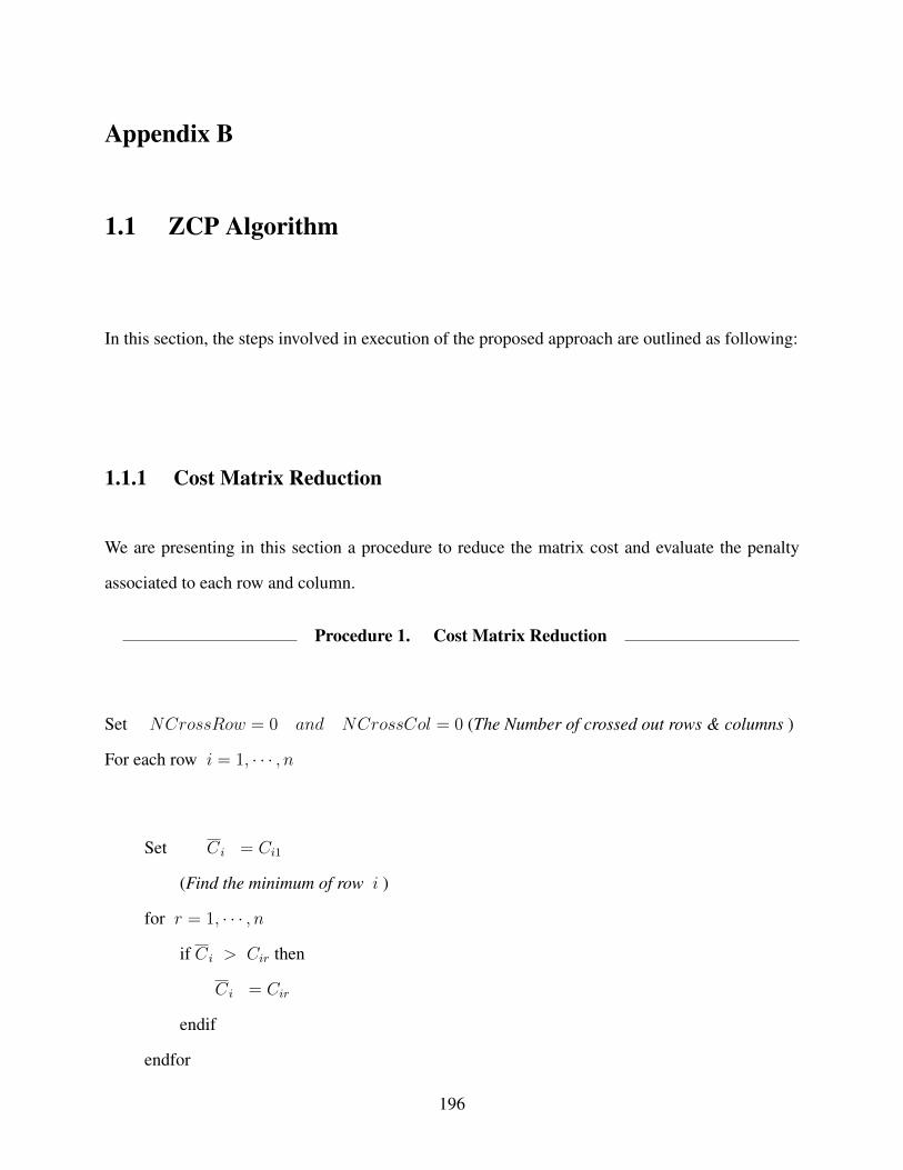
Appendix B
1.1 ZCP Algorithm
In this section, the steps involved in execution of the proposed approach are outlined as following:
1.1.1 Cost Matrix Reduction
We are presenting in this section a procedure to reduce the matrix cost and evaluate the penalty
associated to each row and column.
Procedure 1. Cost Matrix Reduction
Set NCrossRow = 0 and NCrossCol = 0 (The Number of crossed out rows & columns )
For each row i = 1, · · · , n
Set Ci = Ci1
(Find the minimum of row i )
for r = 1, · · · , n
if Ci > Cir then
Ci = Cir
endif
endfor
196

(Reduce the row i )
for j = 1, · · · , n then
Set Rij = Cij − minj{Cij} = Cij − Ci
if Rij = 0 then set
NZRow(i) := NZRow(i) + 1 (Number of zero of row i )
ZRow(i) := ZRow(i) ∪ {j} (Set of zero of row i )
NZCol(j) := NZCol(j) + 1 (Number of zero of column j )
ZCol(j) := ZCol(j) ∪ {i} (Set of zero of column j )
Redcol(j) := 1 (Indicates column j is reduced)
endif
endfor
endFor
For each column j = 1, · · · , n
If Redcol(j) = 1 then
if NZCol(j) ≥ 2 then
Pencol(j) := 0
EPcol(j) := 1 (Indicates that penalty of column j is evaluated)
else
Pencol(j) = mini{Rij : Rij 6= 0}
endif
else
find mini{Rij} = Rkj = Rj
197

Then
Set Rij = Rij −mini{Rij} = Rij − Rj
if Rij = 0 then set
NZRow(i) := NZRow(i) + 1 (Number of zero of row i )
ZRow(i) := ZRow(i) ∪ {j} (Set of zero of row i )
ZCol(j) := ZCol(j) ∪ {i} (Set of zero of column j )
NZCol(j) := NZCol(j) + 1 (Number of zero of column j )
Penrow(i) := 0
EProw(i) := 1 (Indicates that penalty of row i is evaluated)
endif
if NZCol(j) ≥ 2 then
Pencol(j) := 0
else
Pencol(j) = mini{Rij : Rij 6= 0}
endif
endIf
endFor
For each row i = 1, · · · , n
If EProw(i) = 0 then
Penrow(i) = minj{Rij : Rij 6= 0}
endIf
endFor
Set Nred = 1 (Indicate the Number of Reduction for the matrix )
198

1.1.2 Determining the Assigned Variables
To determine the assigned row we consider all the zero case penalties k such that
Zpen = ZPen(k) = Penrow(k) + Pencol(kc)
For each of these lines, the zero cell should be defined. Break the ties, If found, by choosing the
variable with the lowest initial cost. We use the following procedure.
Procedure 2. Determining Variable
For each row r = 1, · · · , n then
If crossrow(r) = 0
if Penrow(r) = 0
there is at least two zeros at the row r, then
we compare the associated column penalties.
then evaluate ZPen(r) by computing the difference between the largest and the sec-
ond largest.
else ( Penrow(r) not null )
if Pencol(rc) = 0
there is at least two zeros at the column rc, then
we compare the associated row penalties.
then set ZPen of the largest row penalty after subtracting the second largest.
then set the ZPen associates with other zeros to be null.
199

else
Set ZPen(r) = pr + qrc
endif
endFor
Find the following parameters
LZPen = maxi{ZPen(i)}
If there us multiple ZPen, then Call procedure 3.
1.1.2.1 Multiple largest penalties
Procedure 3. Multiple Penalties
we consider the case when there are multiple largest penalties for the zeros.
therefore, there are multiple cases have to be considered. Section ?? provides some rules help to
choose the assignment line.
1.1.3 Assigning Variables
Once the variable is determined, we assign Xr,rc and cross out the associated row and column.
200

Procedure 4. Assigning Row
For the variable Xt,z
Set Xt,z = at
Set crossrow(t) = 1
bz = bz − at ( updating the demand)
Zrow(t) = Zrow(t)− {z}
Zcol(z) = Zcol(z)− {t}
NCrossRow = NCrossRow + 1
Procedure 5. Assigning Column
For the variable Xt,z
Set Xt,z = bz
Set crosscol(z) = 1
at = at − bz ( updating the supply)
Zrow(t) = Zrow(t)− {z}
Zcol(z) = Zcol(z)− {t}
NCrossCol = NCrossCol + 1
we consider the situation where pt and qz for the variable Xt,z are equal.
Procedure 6. Equality Case
For the variable Xt,z
Set Xt,z = qz = pt
Set crossrow(t) = 1 and crosscol(z) = 1
201

Zrow(t) = Zrow(t)− {z}
Zcol(z) = Zcol(z)− {t}
NCrossRow = NCrossRow + 1
NCrossCol = NCrossCol + 1
1.1.4 Reduction
1.1.4.1 Null Column Penalty
We consider the situation where
LZPen = ZPen(k) = Penrow(r) + Pencol(rc), such that qrc = 0
Procedure 7. Row Reduction
If qrc = 0 (then there is other zero, at least one on Zcol(rc) )
Zcol(rc) = Zcol(rc)− k (updating the set Zcol(rc) after assigning Xk,rc )
For each s ∈ Zcol(rc)
If Penrow(s) > 0 then (reduce the row s )
for each column j = 1, · · · , n in the row s
if crosscol(j) = 0 then
Rsj = Rsj − penroww(s)
If Rsj = 0 then set
ZRow(s) := ZRow(s) ∪ {j}
NZRow(s) := NZRow(s) + 1 (updating the number of zeros in the row s)
202

NZCol(j) := NZCol(j) + 1 (updating the number of zeros in the column
j)
if NZCol(j) ≥ 2 then
Set qj = 0
else
if Rsj < qj then (updating the column j penalty)
Set qj = Rsj
endif
endIf
endfor
endIf
endFor
Nred := Nred + 1
endIf
1.1.4.2 Null Row Penalty
We consider the situation where
LZPen = ZPen(r) = Penrow(r) + Pencol(rc), such that pr = 0
Procedure 8. Column Reduction
If pr = 0 (then there is other zero, at least one on Zrowl(r) )
Zrow(r) = Zrow(r)− {s} (updating the set Zrow(r) after assigning Xr,s )
For each s ∈ Zrow(r)
203

If Pencol(s) > 0 then (reduce the column s )
for each row i = 1, · · · , n
if crossrow(i) = 0 then
Ris = Ris − pencol(s)
If Ris = 0 then set
ZRow(i) := ZRow(i) ∪ {s}
NZRow(i) := NZRow(i) + 1 (updating the number of zeros in the row i)
NZCol(s) := NZCol(s) + 1 (updating the number of zeros in the column
s)
if NZRow(i) ≥ 2 then
Set pi = 0
else
if Ris < pi then
Set pi = Ris
endif
endIf
endfor
endIf
endFor
Nred := Nred + 1
endIf
204

1.1.5 Updating Penalty
Some of the row and column penalties need to be re-evaluated after each assignment. Assuming
that Xkr is the assigned variable.
1.1.5.1 Row Penalty Evaluation
Procedure 9. Updating Row Penalties
For each row i = 1, · · · , n do
If crossrow(i) = 0 then
if Ri,rc ≤ pi then
if NZRow(i) ≥ 2 then
Set pi = 0
else
Find min{Ri,j / Ri,j 6= 0}
Set pi = min Ri,j
endIf
endFor
endif
endIf
endFor
1.1.5.2 Column Penalty Evaluation
Procedure 10. Updating Column Penalties
205

For each column j = 1, · · · , n do
If crosscol(j) = 0 then
if Rr,j ≤ qj then
if NZCol(j) ≥ 2 then
Set qj = 0
else
Find min{Ri,j / Ri,j 6= 0}
Set qj = min Ri,j
endIf
endFor
endif
endIf
endFor
1.1.6 General algorithm
Step 1. Cost Matrix Reduction
Call procedure 1. Cost Matrix Reduction
Step 2. Determined the assigned Variables
Call procedure 2. Determining variables
if ar < brc then
Call procedure 4. Assigning Row
206
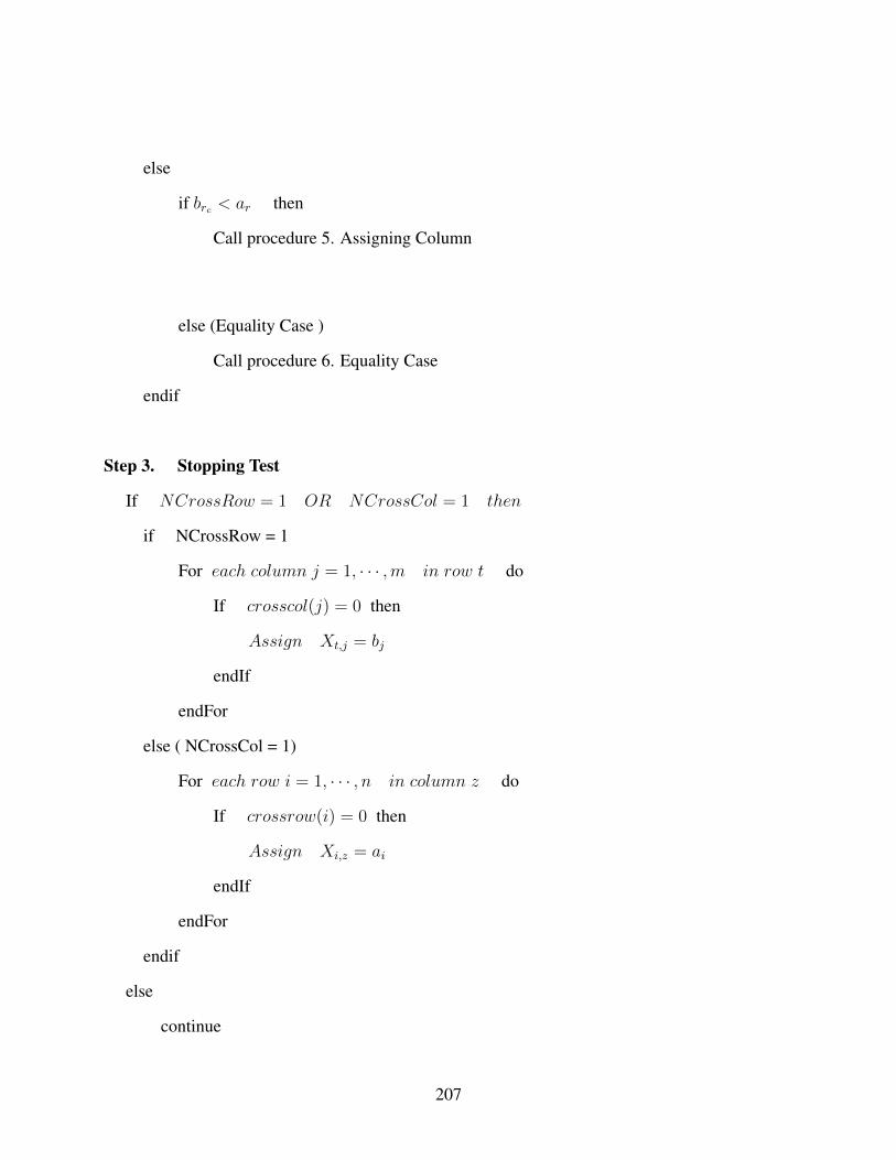
else
if brc < ar then
Call procedure 5. Assigning Column
else (Equality Case )
Call procedure 6. Equality Case
endif
Step 3. Stopping Test
If NCrossRow = 1 OR NCrossCol = 1 then
if NCrossRow = 1
For each column j = 1, · · · ,m in row t do
If crosscol(j) = 0 then
Assign Xt,j = bj
endIf
endFor
else ( NCrossCol = 1)
For each row i = 1, · · · , n in column z do
If crossrow(i) = 0 then
Assign Xi,z = ai
endIf
endFor
endif
else
continue
207

endIf
Step 4. Updating penalties
If Procedure 4 is called then
Call procedure 7. Row Reduction
Call procedure 9. Updating Row Penalties
else
If Procedure 5 is called then
Call procedure 8. Column Reduction
Call procedure 10. Updating Column Penalties
else
If Procedure 6 is called then
if the assigned line is a row then
Call procedure 7. Row Reduction
Call procedure 8. Column Reduction
Call procedure 9. Updating Row Penalties
Call procedure 10. Updating Column Penalties
Step 5. Parameter Updating
go to step 2
Step 6. Optimality Test
If Nred = 1 then the MVM solution is optimal.
Else
208

find the dual variables and test the optimality.
1.2 Special Cases for Multiple Largest Penalties
During the procedure of ZCP, a tie can take a place between the zero penalties. Therefore, there are
some rules help to break the tie and select a good assignment.
1.2.1 Largest Penalty Paralleled lines
We consider the situation where there two lines k and s such that
LZPen(k) = LZPen(s)
Where is zero Rk,kc = 0 on the line k has the penalty Penrow(k) + Pencol(kc). Similarly, the
zero Rs,sc = 0 on the line s has the penalty Penrow(s) + Pencol(sc).
we are considering two cases:
1.2.1.1 Same complementary column
In this case, the two rows have the same complementary column:
Rk,kc = 0 Rs,sc = 0 with kc = sc
209

Case 1. ak + as ≤ bkc
Assign Xk,kc = ak and cross out row k .
Set bkc = bkc − ak
then assign Xk,kc = as and cross out row s
If ak + as = bkc then cross out column kc
else
Set bkc = bkc − as
Update the penalties of the rows and column.
Case 2. ak + as > bkc
Let b1 be the demand associated with the complementarity column k2 containing the reduced
cost pk of the row k
Let b2 be the demand associated with the complementarity column s2 containing the reduced
cost ps of the row s
Let b = max{b2}
Case 2.1 ak ≤ bkc and as ≤ bkc
First we need to compare the left over with the demands b1 and b2
If ak + as − bkc ≤ b = b2
Assign Xk,kc = ak and cross out row k .
Then assign Xs,kc = bkc − ak and Xs,s2 = ak + as − bkc
cross out row s and column kc
Reduce if necessary the remaining rows that contain their zeros in column kc
210

Update if necessary the row penalties.
If ak + as − bkc ≤ b = b1
Assign Xs,kc = as and cross out row s .
Then assign Xk,kc = bkc − as and Xk,k2 = ak + as − bkc
cross out row k and column kc
Reduce if necessary the remaining rows that contain their zeros in column kc
Update if necessary the row penalties.
If ak + as − bkc > b
Find φk the third largest reduced cost of row k
Find φs the third largest reduced cost of row s
Define the costs:
F (k) = ps b2 + (ak + as − bkc − b2)φs and
F (s) = pk b1 + (ak + as − bkc − b1)φk
If F (k) ≤ F (s)
Assign Xk,kc = ak and cross out row k .
Then assign Xs,kc = bkc − ak and Xs,s2 = ak + as − bkc
cross out row s and column kc
Reduce if necessary the remaining rows that contain their zeros in column kc
Update if necessary the row penalties.
else
Assign Xs,kc = as and cross out row s .
Then assign Xk,kc = bkc − as and Xk,k2 = ak + as − bkc
cross out row k and column kc
Reduce if necessary the remaining rows that contain their zeros in column kc
211

Update f necessary the row penalties.
Endif
Case 2.2 ak ≤ bkc and as > bkc
We need to check if there is remaining supplies on row k and s after assigning the largest
penalties.
Define the parameters
Mk = max{0, as + ak − bkc − b2}
Ms = max{0, as − bkc − b2} + max{0, ak − b1}
If Mk > Ms
Assign Xk,kc = ak and cross out row k .
Then assign Xs,kc = bkc − ak and Xs,s2 = min{b2, ak + as − bkc}
cross out column kc and other rows or columns with zero supply or demand
Reduce if necessary the remaining matrix
Update if necessary the penalties.
else
Assign Xs,kc = bkc and cross out column kc .
Then assign Xk,k2 = min{b1, ak} and Xs,s2 = min{b2, as − bkc}
cross out rows or columns with zero supply and demand
Reduce if necessary the remaining matrix
Update f necessary the penalties.
Endif
Case 2.3 ak > bkc and as ≤ bkc
212

We need to check if there is remaining supplies on row k and s after assigning the largest
penalties.
Define the parameters
Mk = max{0, ak − bkc − b1} + max{0, as − b2}
Ms = max{0, ak + as − bkc − b1}
If Mk ≥Ms
Assign Xk,kc = bkc and cross out column kc .
Then assign Xk,k2 = min{b1, ak − bk−c} and Xs,s2 = min{b2, as}
cross out rows or columns with zero supply and demand
Reduce if necessary the remaining matrix
Update f necessary the penalties.
else
Assign Xs,kc = as and cross out row s .
Then assign Xk,kc = bkc − as and Xk,k2 = min{b1, ak + as − bkc}
cross out column kc and other rows or columns with zero supply or demand
Reduce if necessary the remaining matrix
Update if necessary the penalties.
Endif
Case 2.4 ak > bkc and as > bkc
Define the parameters
Mk = max{0, ak − bkc − b1} + max{0, as − b2}
Ms = max{0, as − bkc − b2} + max{0, ak − b1}
If Mk > Ms
213

Assign Xk,kc = bkc and cross out column kc .
Then assign Xk,k2 = min{b1, ak − bk−c} and Xs,s2 = min{b2, as}
cross out rows or columns with zero supply and demand
Reduce if necessary the remaining matrix
Update f necessary the penalties.
else
Assign Xs,kc = bkc and cross out column kc .
Then assign Xk,k2 = min{b1, ak} and Xs,s2 = min{b2, as − bkc}
cross out rows or columns with zero supply and demand
Reduce if necessary the remaining matrix
Update f necessary the penalties.
Endif
1.2.1.2 Different Complementary Columns
In this case, the two rows have different complementary columns.Since analysis for two columns
are similar, we consider the situation two rows
Rk,kc = 0 Rs,sc = 0 with kc 6= sc
If Penrow(k) = 0 OR Pencol(kc) = 0 then
we consider row k by assigning Xk,kc = min{ak, bkc}
Adjust the supply or demand.
Then we reduce if necessary the row k or column kc .
Update the penalties of the rows and columns.
214

If Penrow(s) = 0 OR Pencol(sc) = 0 then
we consider row s by assigning Xs,sc = min{as, bsc}
Adjust the supply or demand.
Then we reduce if necessary the row s or column sc .
Update the penalties of the rows and columns.
else
Case 1. If ak ≤ bkc and as ≤ bsc then
If Pencol(kc) > Pencol(sc) then
Assign row k , Xk,kc = ak and cross out row k.
If ak = bkc assign zero to the least cost of column kc and Cross out column kc
Set bkc = bkc − ak
Then we reduce if necessary the column kc.
Update the penalties of the rows and columns.
else
If Pencol(sc) > Pencol(kc) then
Assign row s , Xs,sc = as and cross out row s.
If as = bsc assign zero to the least cost of column sc and Cross out column sc
Set bsc = bsc − as
Then we reduce if necessary the column sc .
Update the penalties of the rows and columns.
else
215

Compare the left over values bkc − ak and bsc − as
Assign the line associated with the largest value.
Cross out the row or column with zero supply or demand.
Reduce if necessary the remain matrix.
endif
Case 2. If ak ≤ bkc and as > bsc then
If Penrow(s) > Pencol(kc) then
Assign row k , Xk,kc = ak and cross out row k.
If ak = bkc assign zero to the least cost of column kc and Cross out column kc
Set bkc = bkc − ak
Then we reduce if necessary the column kc.
Update the penalties of the rows and columns.
else
If Penrow(s) > Pencol(kc) then
Assign row s , Xs,sc = bsc and cross out column sc.
Set as = as − bsc
Then we reduce if necessary the row s .
Update the penalties of the rows and columns.
else
Compare the left over values bkc − ak and as − bsc
Assign the line associated with the largest value.
Cross out the row or column with zero supply or demand.
Reduce if necessary the remain matrix.
216

endif
Case 3. If ak > bkc and as ≤ bsc then
If Penrow(k) > Pencol(sc) then
Assign row k , Xk,kc = bkc and cross out column kc.
Set ak = ak − bkc
Then we reduce if necessary the row k.
Update the penalties of the rows and columns.
else
If Penrow(k) > Pencol(sc) then
Assign row s , Xs,sc = as and cross out row s.
If as = bsc assign zero to the least cost of column sc and Cross out column sc
Set bsc = bsc − as
Then we reduce if necessary the column sc .
Update the penalties of the rows and columns.
else
Compare the left over values bsc − as and ak − bkc
Assign the line associated with the largest value.
Cross out the row or column with zero supply or demand.
Reduce if necessary the remain matrix.
endif
Case 4. If ak > bkc and as > bsc then
217

If Penrow(k) > Penrow(s) then
Assign row k , Xk,kc = bkc and cross out column kc.
Set ak = ak − bkc
Then we reduce if necessary the row k.
Update the penalties of the rows and columns.
else
If Penrow(s) > Penrow(k) then
Assign row s , Xs,sc = bsc and cross out column sc.
Set as = as − bsc
Then we reduce if necessary the row s .
Update the penalties of the rows and columns.
else
Compare the left over values ak − bkc and as − bsc
Assign the line associated with the largest value.
Cross out the row or column with zero supply or demand.
Reduce if necessary the remain matrix.
endif
218

1.3 Java Code
In this section, we present the Java code of ZCP.
p u b l i c c l a s s ZCProw {
p r i v a t e s t a t i c double [ ] [ ] m a t r i x ;
p r i v a t e s t a t i c double [ ] [ ] c o s t ;
p r i v a t e s t a t i c double [ ] [ ] x ; / / t h e s o l u t i o n m a t r i x
p r i v a t e s t a t i c i n t [ ] [ ] ZPos ;
p r i v a t e s t a t i c double [ ] p ; / / row p e n a l t i e s
p r i v a t e s t a t i c double [ ] q ; / / column p e n a l t i e s
p r i v a t e s t a t i c double [ ] sumP ; / / z e r o p e n a l t i e s
p r i v a t e s t a t i c i n t [ ] dm ; / / column demands
p r i v a t e s t a t i c i n t [ ] sp ; / / row s u p p l i e s
p r i v a t e s t a t i c i n t [ ] crossRows ; / / d e l e t e d rows ( z e r o i f n o t c r o s s e d o u t )
p r i v a t e s t a t i c i n t [ ] c rossColumns ; / / d e l e t e d columns
p r i v a t e s t a t i c i n t [ ] NZRow; / / number o f z e r o s i n each row
p r i v a t e s t a t i c i n t [ ] NZCol ; / / number o f z e r o s i n each column
p r i v a t e s t a t i c i n t [ ] sumpass ; / / i n d i c a t e t h e e v a l u a t e d row p e n a l t i e s
p r i v a t e s t a t i c i n t [ ] pAColumn ; / / i n d i c a t e t h e p o s i t i o n o f column
p e n a l t i e s
p r i v a t e s t a t i c i n t [ ] RedCol ; / / i n d i c a t e t h e reduced columns
p r i v a t e s t a t i c i n t [ ] EPRow ; / / i n d i c a t e t h e e v a l u a t e d row p e n a l t i e s
p r i v a t e s t a t i c double LPen ; / / i n d i c a t e t h e h i g h e s t p e n a l t y
p r i v a t e s t a t i c double sum ;
p r i v a t e s t a t i c double sumSup ; / / sum o f t h e t o t a l s u p p l y
p r i v a t e s t a t i c double sumDem ; / / sum o f t h e t o t a l demand
p r i v a t e s t a t i c i n t NCrossRows , NCrossCols , pARow , column ;
s t a t i c i n t TC ; / / t h e t o t a l s h i p p i n g c o s t
219

p r i v a t e s t a t i c i n t n ,m , var , RedNum ;
p r i v a t e s t a t i c DecimalFormat d f ;
p r i v a t e s t a t i c boolean S o l O p t i m a l ;
/∗ ∗
∗ The R e d u c t i o n F u n c t i o n − column−row R e d u c t i o n
∗ /
p u b l i c s t a t i c vo id M a t r i x R e d u c t i o n ( ) {
RedNum++;
f o r ( i n t i =0 ; i<n ; i ++){
double rowMin= c o s t [ i ] [ 0 ] ;
f o r ( i n t j =1 ; j<m ; j ++){
i f ( c o s t [ i ] [ j ]< rowMin )
rowMin= c o s t [ i ] [ j ] ;
}
/ / t h e n s u b t r a c t t h e min from each c o s t
f o r ( i n t k =0; k<m ; k ++){
c o s t [ i ] [ k ] = c o s t [ i ] [ k]− rowMin ;
i f ( c o s t [ i ] [ k ]==0) {
NZRow[ i ] + + ; / / i n c r e m e n t t h e number o f z e r o s i n row i
NZCol [ k ] + + ; / / i n c r e m e n t t h e number o f z e r o s i n column k
RedCol [ k ] = 1 ; / / column k has been reduced
ZPos [ i ] [ k ] = 1 ; / / mark t h e p o s i t i o n
}
}
}
/ / co lumns
f o r ( i n t j =0 ; j<m; j ++){
i f ( RedCol [ j ]==1) {
i f ( NZCol [ j ] >=2){
220

q [ j ] = 0 ;
}
e l s e {
double colMin= sum ;
/ / c h o o s i n g t h e minimum v a l u e
f o r ( i n t i =0 ; i<n ; i ++){
i f ( c o s t [ i ] [ j ]< colMin && c o s t [ i ] [ j ] ! = 0 )
colMin= c o s t [ i ] [ j ] ;
}
q [ j ]= colMin ;
}
}
e l s e { / / i f t h e column n o t reduced
double colMin= c o s t [ 0 ] [ j ] ;
/ / c h o o s i n g t h e minimum v a l u e
f o r ( i n t i =0 ; i<n ; i ++){ / / i =0
i f ( c o s t [ i ] [ j ]< colMin )
colMin= c o s t [ i ] [ j ] ;
}
double [ ] m i n L i s t = new double [ n ] ;
f o r ( i n t k =0; k<n ; k ++){
c o s t [ k ] [ j ] −= colMin ;
m i n L i s t [ k ]= c o s t [ k ] [ j ] ;
i f ( c o s t [ k ] [ j ]==0) {
NZRow[ k ] + + ;
NZCol [ j ] + + ; / / i n c r e m e n t t h e number o f z e r o s i n column k
p [ k ] = 0 ; / / r ecompute t h e row p e n a l t y
EPRow[ k ] = 1 ; / / mark t h e e v a l u a t e d p e n a l t y
ZPos [ k ] [ j ] = 1 ;
}
}
A rr ay s . s o r t ( m i n L i s t ) ;
221

q [ j ]= m i n L i s t [ 1 ] ;
} / / end e l s e
} / / e n d f o r
/ / c a l c u l a t e t h e row p e n a l t i e s
f o r ( i n t i =0 ; i<n ; i ++){
/ / i f t h e row p e n a l t y n o t e v a l u a t e d
i f ( EPRow[ i ] ! = 1 ) {
i f (NZRow[ i ] >=2){
p [ i ] = 0 ;
}
e l s e {
/ / o t h e r w i s e , i f t h e p e n a l t i e s v a l u e s o t h e r than z e r o s
double rowMin= sum ; / / sum ;
/ / c h o o s i n g t h e minimum v a l u e
f o r ( i n t j =0 ; j<m ; j ++){ / / i =0
i f ( c o s t [ i ] [ j ]< rowMin && c o s t [ i ] [ j ] ! = 0 )
rowMin= c o s t [ i ] [ j ] ;
i f ( ZPos [ i ] [ j ]==1)
pAColumn [ i ]= j ; / / z e r o p o s i t i o n
}
p [ i ]= rowMin ;
} / / end e l s e
}
} / / end f o r
}
/∗ ∗
∗ T h i s f u n c t i o n d e t e r m i n e s t h e a s s i g n i n g v a r i a b l e s
∗ /
p u b l i c s t a t i c vo id C o n s i d e r i n g V a r i a b l e ( ) {
222
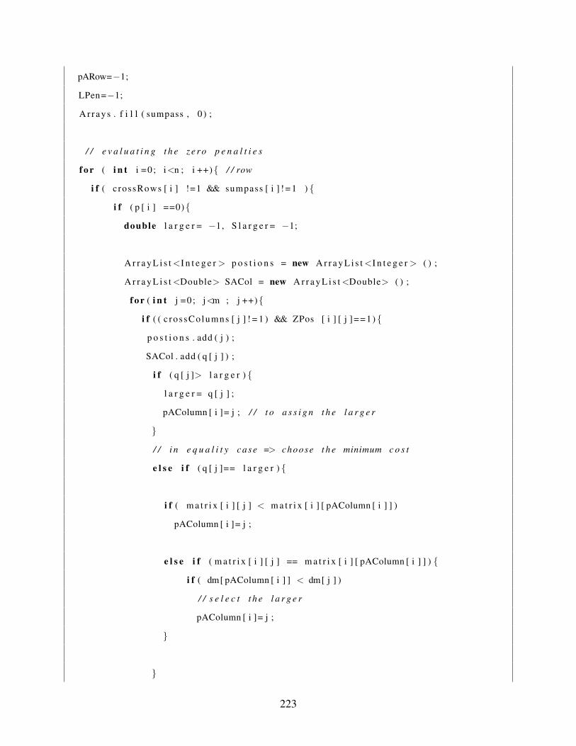
pARow=−1;
LPen=−1;
A r r ay s . f i l l ( sumpass , 0 ) ;
/ / e v a l u a t i n g t h e z e r o p e n a l t i e s
f o r ( i n t i =0 ; i<n ; i ++){ / / row
i f ( crossRows [ i ] !=1 && sumpass [ i ] ! = 1 ) {
i f ( p [ i ] ==0){
double l a r g e r = −1, S l a r g e r = −1;
A r r a y L i s t<I n t e g e r > p o s t i o n s = new A r r a y L i s t<I n t e g e r > ( ) ;
A r r a y L i s t<Double> SACol = new A r r a y L i s t<Double> ( ) ;
f o r ( i n t j =0 ; j<m ; j ++){
i f ( ( c rossColumns [ j ] ! = 1 ) && ZPos [ i ] [ j ]==1) {
p o s t i o n s . add ( j ) ;
SACol . add ( q [ j ] ) ;
i f ( q [ j ]> l a r g e r ) {
l a r g e r = q [ j ] ;
pAColumn [ i ]= j ; / / t o a s s i g n t h e l a r g e r
}
/ / i n e q u a l i t y case => choose t h e minimum c o s t
e l s e i f ( q [ j ]== l a r g e r ) {
i f ( m a t r i x [ i ] [ j ] < m a t r i x [ i ] [ pAColumn [ i ] ] )
pAColumn [ i ]= j ;
e l s e i f ( m a t r i x [ i ] [ j ] == m a t r i x [ i ] [ pAColumn [ i ] ] ) {
i f ( dm[ pAColumn [ i ] ] < dm[ j ] )
/ / s e l e c t t h e l a r g e r
pAColumn [ i ]= j ;
}
}
223

}
}
C o l l e c t i o n s . s o r t ( SACol ) ;
S l a r g e r = SACol . g e t ( SACol . s i z e ( ) −2) ;
sumP [ i ] = l a r g e r − S l a r g e r ;
}
e l s e { / / p [ i ] !=0
sumP [ i ] = q [ pAColumn [ i ] ] ;
i f ( q [ pAColumn [ i ] ] ==0 ) {
double l a r g e r =0 , S l a r g e r =0 ;
A r r a y L i s t<Double> RowPen = new A r r a y L i s t<Double> ( ) ;
A r r a y L i s t<I n t e g e r > RowPos i t ion = new A r r a y L i s t<I n t e g e r > ( ) ;
/ /
RowPen . add ( p [ i ] ) ;
RowPos i t ion . add ( i ) ;
f o r ( i n t r =0 ; r<n ; r ++){
i f ( crossRows [ r ] !=1 && ZPos [ r ] [ pAColumn [ i ] ] = = 1 ) {
i f ( r != i && p [ r ] ! = 0 ) {
RowPen . add ( p [ r ] ) ;
RowPos i t ion . add ( r ) ;
}
}
} / / end f o r
i f ( RowPen . s i z e ( ) >=2){
C o l l e c t i o n s . s o r t ( RowPen ) ;
l a r g e r = RowPen . g e t ( RowPen . s i z e ( ) −1) ;
S l a r g e r = RowPen . g e t ( RowPen . s i z e ( ) −2) ;
224

/ / t h e p e n a l t y o f z e r o i s t h e d i f f e r e n c e be tween
/ / t h e l a r g e s t and t h e second l a r g e s t
f o r ( i n t r : RowPos i t ion ) {
i f ( p [ r ] == l a r g e r ) {
sumP [ r ] = l a r g e r − S l a r g e r ;
}
e l s e {
sumP [ r ] = 0 ;
/ / marked
sumpass [ r ] = 1 ;
}
}
}
e l s e { / / RowPen . s i z e ( )< 2
sumP [ i ] = p [ i ] ;
}
}
e l s e { / / q !=0
sumP [ i ] += p [ i ] ;
}
} / / end e l s e
/ / c o n s i d e r t h e l a r g e s t p e n a l t y
i f ( sumP [ i ]> LPen ) {
LPen=sumP [ i ] ;
pARow= i ;
}
e l s e i f ( sumP [ i ]== LPen ) {
/ / t h e same complementary column
i f ( ( pAColumn [ i ] == pAColumn [pARow ] ) && m−NCrossCols >= 3) {
/ / 2 c a s e s
/ / i f ( sp [ i ] +sp [pARow] <= dm[ pAColumn ] ) {
225

/ / s i m u l t a n e o u s l y
i f ( sp [ i ] +sp [pARow] > dm[ pAColumn [ i ] ] ) {
/ / 4 subcases , 2 unchangeab le
i n t b1=−1 , b2=−1, max=−1;
A r r a y L i s t<Double> min1= new A r r a y L i s t<Double >() ;
A r r a y L i s t<Double> min2 = new A r r a y L i s t<Double >() ;
double ph i1 =0 , ph i2 =0 , fpARow , f i ;
f o r ( i n t c =0; c<m; c ++){
i f ( c rossColumns [ c ] ! = 1 && c != pAColumn [pARow ] ) {
min1 . add ( c o s t [pARow ] [ c ] ) ;
min2 . add ( c o s t [ i ] [ c ] ) ;
i f ( c o s t [pARow ] [ c ]== p [pARow ] )
b1=c ;
i f ( c o s t [ i ] [ c ]== p [ i ] )
b2=c ;
}
} / / end f o r
C o l l e c t i o n s . s o r t ( min1 ) ;
C o l l e c t i o n s . s o r t ( min2 ) ;
ph i1 = min1 . g e t ( 1 ) ; / / phi−k / / 2
ph i2 = min2 . g e t ( 1 ) ; / / phi−s / / 2
i f (dm[ b1 ] >= dm[ b2 ] )
max =0; / / b1
e l s e
max =1; / / b2
i f ( sp [pARow] <= dm[ pAColumn [ i ] ] && sp [ i ] <= dm[ pAColumn [ i ] ] ) { / / 1
i f ( max==0 && ( sp [pARow]+ sp [ i ]−dm[ pAColumn [ i ] ] ) <= dm[ b1 ] ) {
pARow= i ;
}
226
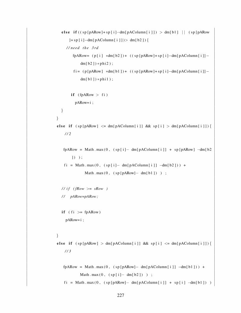
e l s e i f ( ( sp [pARow]+ sp [ i ]−dm[ pAColumn [ i ] ] ) > dm[ b1 ] | | ( sp [pARow
]+ sp [ i ]−dm[ pAColumn [ i ] ] )> dm[ b2 ] ) {
/ / need t h e 3 rd
fpARow= ( p [ i ] ∗dm[ b2 ] ) + ( ( sp [pARow]+ sp [ i ]−dm[ pAColumn [ i ]]−
dm[ b2 ] ) ∗ ph i2 ) ;
f i = ( p [pARow] ∗dm[ b1 ] ) + ( ( sp [pARow]+ sp [ i ]−dm[ pAColumn [ i ]]−
dm[ b1 ] ) ∗ ph i1 ) ;
i f ( fpARow > f i )
pARow= i ;
}
}
e l s e i f ( sp [pARow] <= dm[ pAColumn [ i ] ] && sp [ i ] > dm[ pAColumn [ i ] ] ) {
/ / 2
fpARow = Math . max ( 0 , ( sp [ i ]− dm[ pAColumn [ i ] ] + sp [pARow] −dm[ b2
] ) ) ;
f i = Math . max ( 0 , ( sp [ i ]− dm[ pAColumn [ i ] ] −dm[ b2 ] ) ) +
Math . max ( 0 , ( sp [pARow]− dm[ b1 ] ) ) ;
/ / i f ( fRow >= sRow )
/ / pARow=pARow ;
i f ( f i >= fpARow )
pARow= i ;
}
e l s e i f ( sp [pARow] > dm[ pAColumn [ i ] ] && sp [ i ] <= dm[ pAColumn [ i ] ] ) {
/ / 3
fpARow = Math . max ( 0 , ( sp [pARow]− dm[ pAColumn [ i ] ] −dm[ b1 ] ) ) +
Math . max ( 0 , ( sp [ i ]− dm[ b2 ] ) ) ;
f i = Math . max ( 0 , ( sp [pARow]− dm[ pAColumn [ i ] ] + sp [ i ] −dm[ b1 ] ) )
227
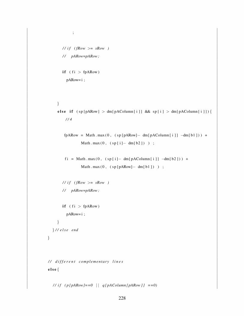
;
/ / i f ( fRow >= sRow )
/ / pARow=pARow ;
i f ( f i > fpARow )
pARow= i ;
}
e l s e i f ( sp [pARow] > dm[ pAColumn [ i ] ] && sp [ i ] > dm[ pAColumn [ i ] ] ) {
/ / 4
fpARow = Math . max ( 0 , ( sp [pARow]− dm[ pAColumn [ i ] ] −dm[ b1 ] ) ) +
Math . max ( 0 , ( sp [ i ]− dm[ b2 ] ) ) ;
f i = Math . max ( 0 , ( sp [ i ]− dm[ pAColumn [ i ] ] −dm[ b2 ] ) ) +
Math . max ( 0 , ( sp [pARow]− dm[ b1 ] ) ) ;
/ / i f ( fRow >= sRow )
/ / pARow=pARow ;
i f ( f i > fpARow )
pARow= i ;
}
} / / e l s e end
}
/ / d i f f e r e n t complementary l i n e s
e l s e {
/ / i f ( p [pARow]==0 | | q [ pAColumn [pARow ] ] ==0)
228

/ / pARow ;
i f ( ( p [pARow] !=0 && q [ pAColumn [pARow ] ] ! = 0 ) && ( p [ i ]==0 | | q [
pAColumn [ i ] ] ==0) ) {
pARow= i ;
}
e l s e {
i f ( sp [pARow] <= dm[ pAColumn [pARow ] ] && sp [ i ] <= dm[ pAColumn [ i ] ] )
{
/ / i f ( q [ pAColumn [pARow ] ] > q [ pAColumn [ i ] ] )
/ / pARow
i f ( q [ pAColumn [ i ] ] > q [ pAColumn [pARow ] ] ) {
pARow= i ;
}
e l s e i f ( q [ pAColumn [pARow ] ] == q [ pAColumn [ i ] ] ) {
i f ( ( dm[ pAColumn [ i ] ] − sp [ i ] ) > (dm[ pAColumn [pARow ] ] − sp [
pARow ] ) ) {
pARow= i ;
}
}
}
e l s e i f ( sp [pARow] <= dm[ pAColumn [pARow ] ] && sp [ i ] > dm[ pAColumn [ i
] ] ) {
i f ( p [ i ] > q [ pAColumn [pARow ] ] ) {
pARow= i ;
}
e l s e i f ( p [ i ] == q [ pAColumn [pARow ] ] ) {
229

i f ( ( sp [ i ] − dm[ pAColumn [ i ] ] ) > (dm[ pAColumn [pARow ] ] − sp [
pARow ] ) ) {
pARow= i ;
}
}
}
e l s e i f ( sp [pARow] > dm[ pAColumn [pARow ] ] && sp [ i ] <= dm[ pAColumn [ i
] ] ) {
i f ( q [ pAColumn [ i ] ] > p [pARow ] ) {
pARow= i ;
}
e l s e i f ( q [ pAColumn [ i ] ] == p [pARow ] ) {
i f ( (dm[ pAColumn [ i ] ] − sp [ i ] ) > ( sp [pARow] − dm[ pAColumn [
pARow ] ] ) ) {
pARow= i ;
}
}
}
e l s e i f ( sp [ i ] > dm[ pAColumn [ i ] ] && sp [pARow] > dm[ pAColumn [pARow
] ] ) {
i f ( p [ i ] > p [pARow ] ) {
pARow= i ;
}
e l s e i f ( p [ i ] == p [pARow ] ) {
i f ( ( sp [ i ] − dm[ pAColumn [ i ] ] ) > ( sp [pARow] − dm[ pAColumn [
pARow ] ] ) ) {
pARow= i ;
230

}
}
}
} / / end e q u a l t y
}
}
} / / end i f
} / / end f o r
}
/∗ ∗
∗ The A s s i g n i n g F u n c t i o n
∗ @param r − row
∗ @param c − column
∗ @param t − t h e minimum v a l u e be tween t h e s u p p l y and demand
∗ /
p u b l i c s t a t i c vo id A s s i g n i n g ( i n t r , i n t c , i n t t ) {
x [ r ] [ c ]= t ∗ m a t r i x [ r ] [ c ] ;
TC+= x [ r ] [ c ] ;
v a r ++;
NZRow[ r ]−−;
NZCol [ c]−−;
}
/∗ ∗
∗ T h i s f u n c t i o n c a l l s t h e r e d u c t i o n f u n c t i o n f o r a column i f needed
∗ @param r − row
∗ @param qc − t h e complementary column
∗ /
p u b l i c s t a t i c vo id RowCrossed ( i n t r , i n t qc ) {
i f ( p [ r ] ==0){
f o r ( i n t j =0 ; j<m; j ++){
231

i f ( c rossColumns [ j ] ! = 1 && ZPos [ r ] [ j ]==1) {
i f ( j != qc ) {
NZRow[ r ]−−;
NZCol [ j ]−−;
i f ( q [ j ] !=0 && NZCol [ j ]==0) { / / i f t h e r e i s a n o t h e r z e r o
ReducingCol ( j ) ;
}
}
}
}
}
i f ( q [ qc ] !=0 && crossColumns [ qc ] ! = 1 ) { / / t h e a s s o c i a t e d column
ReducingCol ( qc ) ;
}
}
/∗ ∗
∗ The R e d u c t i o n F u n c t i o n f o r a column
∗ @param c − column
∗ /
p u b l i c s t a t i c vo id ReducingCol ( i n t c ) {
RedNum++;
f o r ( i n t i =0 ; i<n ; i ++){
i f ( crossRows [ i ] ! = 1 ) {
c o s t [ i ] [ c ]= c o s t [ i ] [ c]−q [ c ] ;
i f ( c o s t [ i ] [ c ] ==0){
ZPos [ i ] [ c ] = 1 ;
NZRow[ i ] + + ;
NZCol [ c ] + + ;
232

/ / u p d a t i n g t h e row p e n a l t y
p [ i ] = 0 ;
}
e l s e i f ( c o s t [ i ] [ c ] < p [ i ] ) / / u p d a t i n g t h e column p e n a l t y
p [ i ]= c o s t [ i ] [ c ] ;
}
}
}
/∗ ∗
∗ T h i s f u n c t i o n c a l l s t h e r e d u c t i o n f u n c t i o n f o r a row i f needed
∗ @param pr − t h e complementary row
∗ @param c − column
∗ /
p u b l i c s t a t i c vo id ColCrossed ( i n t pr , i n t c ) {
i f ( q [ c ] ==0){
f o r ( i n t i =0 ; i<n ; i ++){
i f ( crossRows [ i ] ! = 1 && ZPos [ i ] [ c ]==1) {
i f ( i != p r ) { / / e x c e p t t h e a s s o c i a t e d row
NZRow[ i ]−−;
NZCol [ c]−−;
i f ( p [ i ] !=0 && NZRow[ i ]==0 ) { / / i f t h e row i has a n o t h e r z e r o
ReducingRow ( i ) ;
}
}
}
}
}
i f ( p [ p r ] !=0 && crossRows [ p r ] ! = 1 ) { / / a s s o c i a t e d row
ReducingRow ( pr ) ;
233

}
}
/∗ ∗
∗ The R e d u c t i o n F u n c t i o n f o r a row
∗ @param r − row
∗ /
p u b l i c s t a t i c vo id ReducingRow ( i n t r ) {
RedNum++;
f o r ( i n t j =0 ; j<m ; j ++){
i f ( c rossColumns [ j ] ! = 1 ) {
c o s t [ r ] [ j ]= c o s t [ r ] [ j ]−p [ r ] ;
i f ( c o s t [ r ] [ j ] ==0){
ZPos [ r ] [ j ] = 1 ;
NZRow[ r ] + + ;
NZCol [ j ] + + ;
pAColumn [ r ] = j ;
/ / u p d a t i n g t h e row p e n a l t y
q [ j ] = 0 ;
}
e l s e i f ( c o s t [ r ] [ j ] < q [ j ] ) { / / u p d a t i n g t h e column p e n a l t y
q [ j ]= c o s t [ r ] [ j ] ;
}
}
} / / end f o r
}
234

/∗ ∗
∗ T h i s f u n c t i o n r e c o m p u t e s t h e row p e n a l t i e s
∗ @param pc − column
∗ /
p u b l i c s t a t i c vo id U pd a t in g Ro wP en a l i t y ( i n t pc ) {
f o r ( i n t i =0 ; i<n ; i ++){
i f ( crossRows [ i ] ! = 1 ) {
i f ( c o s t [ i ] [ pc ] <= p [ i ] ) {
i f (NZRow[ i ]>=2){
p [ i ] = 0 ;
}
e l s e {
double min = sum ;
f o r ( i n t j =0 ; j<m ; j ++){
i f ( c rossColumns [ j ] ! = 1 ) {
i f ( c o s t [ i ] [ j ] !=0 && c o s t [ i ] [ j ] < min )
min= c o s t [ i ] [ j ] ;
i f ( ZPos [ i ] [ j ]==1)
pAColumn [ i ]= j ;
}
}
p [ i ]= min ;
}
}
}
}
}
/∗ ∗
∗ T h i s f u n c t i o n r e c o m p u t e s t h e column p e n a l t i e s
235

∗ @param qr − row
∗ /
p u b l i c s t a t i c vo id U p d a t i n g C o l P e n a l i t y ( i n t qr ) {
f o r ( i n t j =0 ; j<m ; j ++){
i f ( c rossColumns [ j ] ! = 1 ) {
i f ( c o s t [ q r ] [ j ] <= q [ j ] ) {
i f ( NZCol [ j ]>=2){
q [ j ] = 0 ;
}
e l s e {
double min = sum ;
f o r ( i n t i =0 ; i<n ; i ++){
i f ( crossRows [ i ] ! = 1 ) {
i f ( c o s t [ i ] [ j ] !=0 && c o s t [ i ] [ j ] < min )
min= c o s t [ i ] [ j ] ;
}
}
q [ j ]= min ;
}
}
}
}
}
/∗ ∗
∗ The s top−case method
∗ /
p u b l i c s t a t i c vo id s t o p C a s e ( ) {
i f ( n−NCrossRows ==1){ / / j u s t one row l e f t
i n t row=−1;
f o r ( i n t i =0 ; i<n ; i ++){
i f ( crossRows [ i ] ! = 1 )
236

row= i ;
}
f o r ( i n t j =0 ; j<m; j ++){
i f ( c rossColumns [ j ] ! = 1 ) {
/ / a s s i g n i n g t h e r e m a i n i n g columns
A s s i g n i n g ( row , j , dm[ j ] ) ;
}
}
}
e l s e i f (m−NCrossCols ==1){ / / one column l e f t
i n t c o l =−1;
f o r ( i n t j =0 ; j<m ; j ++){
i f ( c rossColumns [ j ] ! = 1 )
c o l = j ;
}
f o r ( i n t i =0 ; i<n ; i ++){
i f ( crossRows [ i ] ! = 1 ) {
/ / a s s i g n i n g t h e r e m a i n i n g rows
A s s i g n i n g ( i , co l , sp [ i ] ) ;
}
}
}
}
/∗ ∗
∗ T h i s f u n c t i o n t e s t s i f t h e s o l u t i o n i s o p t i m a l
∗ @return t r u e i f o p t i m a l . Otherwise , f a l s e
∗ /
p u b l i c s t a t i c boolean I s O p t i m a l ( ) {
boolean o p t i m a l = f a l s e ;
i f ( RedNum ==1 )
237

o p t i m a l = t rue ;
re turn o p t i m a l ;
}
/∗ ∗
∗ The Genera l A l g o r i t h m f o r ZCP
∗ @param a r r a y
∗ @param sup
∗ @param dem
∗ /
p u b l i c s t a t i c S t r i n g G e n e r a l A l g o r i t h m ( double [ ] [ ] a r r a y , i n t [ ] sup , i n t [ ]
dem ) {
n= a r r a y . l e n g t h ;
m= a r r a y [ 0 ] . l e n g t h ;
c o s t = new double [ n ] [m] ; / / c o s t m a t r i x
m a t r i x = new double [ n ] [m] ; / / copy t h e c o s t m a t r i x
sp = new i n t [ n ] ;
dm = new i n t [m] ;
sumSup =0; sumDem=0;
f o r ( i n t i =0 ; i<n ; i ++){
f o r ( i n t j =0 ; j<m ; j ++){
i f ( a r r a y [ i ] [ j ] <0)
throw new I l l e g a l A r g u m e n t E x c e p t i o n ( ” t h e c o s t must be p o s t i v e ” ) ;
sum+= a r r a y [ i ] [ j ] ;
}
System . a r r a y c o p y ( a r r a y [ i ] , 0 , c o s t [ i ] , 0 , a r r a y [ i ] . l e n g t h ) ;
238

System . a r r a y c o p y ( a r r a y [ i ] , 0 , m a t r i x [ i ] , 0 , a r r a y [ i ] . l e n g t h ) ;
sp [ i ]= sup [ i ] ;
sumSup+= sp [ i ] ;
}
ZPos = new i n t [ n ] [m] ;
x = new double [ n ] [m] ;
crossRows = new i n t [ n ] ;
c rossColumns = new i n t [m] ;
p = new double [ n ] ;
q = new double [m] ;
NZRow = new i n t [ n ] ;
NZCol = new i n t [m] ;
EPRow = new i n t [ n ] ;
RedCol = new i n t [m] ;
pAColumn= new i n t [ n ] ;
sumpass= new i n t [ n ] ;
sumP= new double [ n ] ;
TC=0;
NCrossRows =0; NCrossCols =0;
RedNum =0; v a r =0;
LPen=−1; column =−1;
d f = new DecimalFormat ( ” # ,### ,### ” ) ;
f o r ( i n t j =0 ; j<m ; j ++){
dm[ j ]= dem [ j ] ;
sumDem+= dm[ j ] ;
}
i f ( sumSup !=sumDem )
throw new I l l e g a l A r g u m e n t E x c e p t i o n ( ” The TP i s n o t b a l a n c e d ” ) ;
239
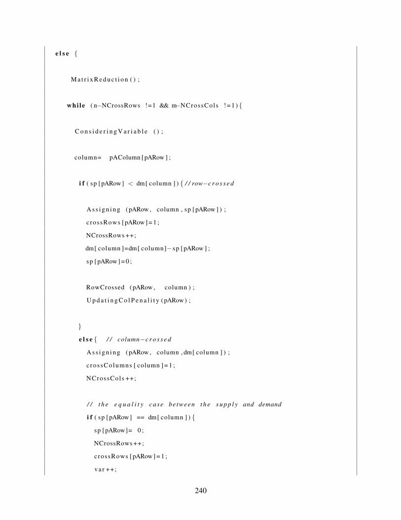
e l s e {
M a t r i x R e d u c t i o n ( ) ;
whi le ( n−NCrossRows !=1 && m−NCrossCols ! = 1 ) {
C o n s i d e r i n g V a r i a b l e ( ) ;
column= pAColumn [pARow ] ;
i f ( sp [pARow] < dm[ column ] ) { / / row−c r o s s e d
A s s i g n i n g (pARow , column , sp [pARow ] ) ;
crossRows [pARow ] = 1 ;
NCrossRows ++;
dm[ column ]=dm[ column]− sp [pARow ] ;
sp [pARow ] = 0 ;
RowCrossed (pARow , column ) ;
U p d a t i n g C o l P e n a l i t y (pARow) ;
}
e l s e { / / column−c r o s s e d
A s s i g n i n g (pARow , column , dm[ column ] ) ;
c rossColumns [ column ] = 1 ;
NCrossCols ++;
/ / t h e e q u a l i t y case be tween t h e s u p p l y and demand
i f ( sp [pARow] == dm[ column ] ) {
sp [pARow]= 0 ;
NCrossRows ++;
crossRows [pARow ] = 1 ;
v a r ++;
240

RowCrossed (pARow , column ) ;
U p d a t i n g C o l P e n a l i t y (pARow) ;
}
e l s e {
sp [pARow]= sp [pARow]−dm[ column ] ;
}
dm[ column ] = 0 ;
Co lCrossed (pARow , column ) ;
U pd a t i n gR o wP en a l i t y ( column ) ;
}
} / / end w h i l e
s t o p C a s e ( ) ;
S o l O p t i m a l = I s O p t i m a l ( ) ;
} / / end e l s e
re turn df . f o r m a t (TC) ;
}
}
241