Neutron emission spectroscopy of fusion plasmas witha NE213 liquid scintillator at JET

Federico Binda

Licentiate ThesisDepartment of Physics and Astronomy

Uppsala University

2015

Abstract

Neutron diagnostics will play a fundamental role in future fusion plasma machines,where the harsh environment will make the use of many other type of diagnos-tics practically impossible. Complex techniques to measure the neutron spectrumemitted from tokamk plasmas have been developed over the years, producing stateof the art neutron spectrometers. However, recently compact neutron spectrom-eters have been gaining the interest of the research community. They are muchsimpler to operate and maintain, have lower cost and they can be employed in thechannels of a neutron camera, providing profile measurements. The drawbacks arethat they have a worse resolution and a response to neutrons that is not optimalfor spectroscopy.

The goal of the work presented in this thesis is to estimate to which extenta compact detector such as a NE213 liquid scintillator can be used to performneutron emission spectroscopy analysis.

The detector used for this study was installed in the back of the MPRu spec-trometer at JET in 2012. The characterization of the response of the detector wasdone using a combination of MCNPX simulations and real measurements. Thedata analysis was performed using the forward fitting approach: a model of theneutron spectrum is produced, then folded with the response of the detector andfinally compared with the data. Two types of plasma scenarios were analyzed, onewith NBI heating only, and another with NBI and third harmonic radio-frequencyheating. In both cases the TOFOR spectrometer was used as a reference to esti-mate the parameters in the model of the neutron spectrum.

The results are promising and suggest that neutron spectroscopy can be per-formed with NE213 scintillators although the quality of the results, as given byperformance indicators such as uncertainties, is much lower than the performanceof high resolution spectrometers.

List of papers

This thesis is based on the following papers

Paper I

Monte carlo simulation of the data acquisition chain of scintillation de-tectors

F. Binda, G. Ericsson, C. Hellesen, A. Hjalmarsson, J. Eriksson, M. Skiba, S.Conroy and M. Weiszflog

Proceedings of the International Conference on Fusion Reactor Diagnostics, Septem-ber, 9–13, 2013, Varenna (LC), Italy. AIP Conf. Proc. 1612 (2014) 101.

My contribution: Developed and tested the code; wrote the paper.

Paper II

Forward fitting of experimental data from a NE213 neutron detector in-stalled with the magnetic proton recoil upgraded spectrometer at JET

F. Binda, G. Ericsson, J. Eriksson, C. Hellesen, S. Conroy, E. Andersson Sundenand JET EFDA Contributors

Proceedings of the 20th Topical Conference on High-Temperature Plasma Diag-nostics, June, 1–5, 2014, Atlanta, Georgia, USA. Rev. Sci. Instrum. 85 (2014)11E123.

My contribution: Performed the calibration, the MCNPX simulations, the dataanalysis and the error estimate; wrote the paper.

Paper III

Analysis of the fast ion tails observed in the NE213 pulse height spectameasured during third harmonic radio-frequency heating experimentsat JET

5

F. Binda, J. Eriksson, G. Ericsson, C. Hellesen, S. Conroy, M. Cecconello, M.Nocente, C. Cazzaniga, E. Andersson Sunden and JET Contributors

Manuscript.

My contribution: Performed the corrections for pile-up, count rate and tritonburn-up; performed the response calculation and the data analysis; wrote the pa-per.

6

Contents

Preface 9

1 Introduction to nuclear fusion 11

2 Magnetically confined fusion 132.1 Tokamak . . . . . . . . . . . . . . . . . . . . . . . . . . . . . . . . . 14

2.1.1 JET . . . . . . . . . . . . . . . . . . . . . . . . . . . . . . . 142.2 Heating methods . . . . . . . . . . . . . . . . . . . . . . . . . . . . 15

3 Fusion neutrons 173.1 Neutron emission spectroscopy . . . . . . . . . . . . . . . . . . . . . 18

4 Neutron diagnostics 194.1 Quality of a neutron spectrometer . . . . . . . . . . . . . . . . . . . 194.2 The magnetic proton recoil technique . . . . . . . . . . . . . . . . . 194.3 TOFOR . . . . . . . . . . . . . . . . . . . . . . . . . . . . . . . . . 204.4 Compact spectrometers . . . . . . . . . . . . . . . . . . . . . . . . . 22

4.4.1 Liquid scintillators . . . . . . . . . . . . . . . . . . . . . . . 224.5 Comparison between spectrometers . . . . . . . . . . . . . . . . . . 24

5 The “Afterburner” installation 275.1 Detector specifications and assembly . . . . . . . . . . . . . . . . . 275.2 Line of sight and Field of view . . . . . . . . . . . . . . . . . . . . . 28

6 Afterburner system characterization 316.1 Typical pulses . . . . . . . . . . . . . . . . . . . . . . . . . . . . . . 316.2 Pulse shape discrimination . . . . . . . . . . . . . . . . . . . . . . . 316.3 MCNPX model . . . . . . . . . . . . . . . . . . . . . . . . . . . . . 346.4 Gamma and neutron calibration . . . . . . . . . . . . . . . . . . . . 36

7 Dacsim - Data acquisition chain simulation (Paper I) 417.1 The code . . . . . . . . . . . . . . . . . . . . . . . . . . . . . . . . . 417.2 Examples . . . . . . . . . . . . . . . . . . . . . . . . . . . . . . . . 42

8 Data analysis 458.1 Data processing . . . . . . . . . . . . . . . . . . . . . . . . . . . . . 45

8.1.1 Gain drift . . . . . . . . . . . . . . . . . . . . . . . . . . . . 45

7

8.1.2 Pile-up rejection . . . . . . . . . . . . . . . . . . . . . . . . 478.2 Analysis of the neutron pulse height spectra . . . . . . . . . . . . . 47

8.2.1 Thermal fraction estimate (Paper II) . . . . . . . . . . . . . 498.2.2 Third harmonic radio-frequency heating analysis (Paper III) 53

9 Conclusions 57

Acknowledgments 59

8

Preface

When I started working on this project, back in 2011, I was still a master student.At the time the idea behind the so-called “Afterburner” installation was to enhancethe time resolution of the neutron flux measurement of the MPRu during DDoperations. After the detector was installed in 2012 and we started collecting data,we realised that there were many other interesting paths that we could explore. Westarted investigating the possibility of performing neutron emission spectroscopyanalysis of the spectra that we had collected. The task was certainly not aneasy one, especially considering that the Afterburner detector was never meantto be used as a spectrometer and therefore its response to neutrons had not beenmeasured. However it was also a very exciting challenge, because such detailedspectroscopy work with a NE213 scintillator had not been attemped before. Wewent down that road and this thesis is the result of all the effort we have put intothis during the last three years.

Federico BindaApril 21, 2015

9

10

1 Introduction to nuclear fusion

The growing world energy demand calls for technologies that can provide clean,cheap and virtually unlimited energy. Nuclear fusion has the potential to fulfillsuch requirements, and is therefore subject to thorough investigation by scientists,in the attempt to find an efficient and practical way to obtain a net energy outputfrom it [1].

The basic principle of fusion is, as the word says, the merging of two nuclei.The products of this process are a heavier nucleus and a light particle. If the totalmass of the products is lower than the total mass of the reactants, the reactiongives a positive energy output, according to the famous relationship:

E = ∆m · c2. (1)

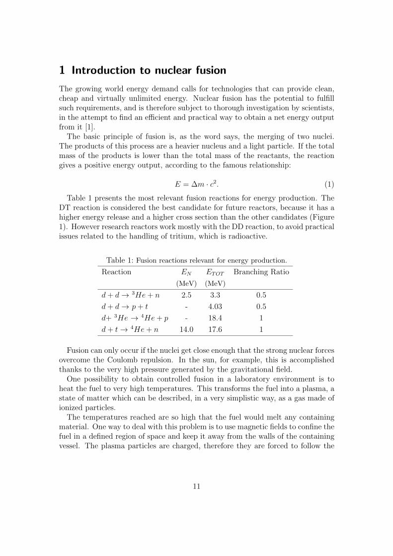
Table 1 presents the most relevant fusion reactions for energy production. TheDT reaction is considered the best candidate for future reactors, because it has ahigher energy release and a higher cross section than the other candidates (Figure1). However research reactors work mostly with the DD reaction, to avoid practicalissues related to the handling of tritium, which is radioactive.

Table 1: Fusion reactions relevant for energy production.

Reaction EN ETOT Branching Ratio

(MeV) (MeV)

d+ d→ 3He+ n 2.5 3.3 0.5

d+ d→ p+ t - 4.03 0.5

d+ 3He → 4He+ p - 18.4 1

d+ t→ 4He+ n 14.0 17.6 1

Fusion can only occur if the nuclei get close enough that the strong nuclear forcesovercome the Coulomb repulsion. In the sun, for example, this is accomplishedthanks to the very high pressure generated by the gravitational field.

One possibility to obtain controlled fusion in a laboratory environment is toheat the fuel to very high temperatures. This transforms the fuel into a plasma, astate of matter which can be described, in a very simplistic way, as a gas made ofionized particles.

The temperatures reached are so high that the fuel would melt any containingmaterial. One way to deal with this problem is to use magnetic fields to confine thefuel in a defined region of space and keep it away from the walls of the containingvessel. The plasma particles are charged, therefore they are forced to follow the

11

magnetic field lines. Magnetically confined fusion is the center of this work andwill be discussed more in detail in the next chapter.

Another way to obtain controlled fusion which is important to mention is inertialconfinement. In inertial confinement fusion the fuel is made into a small pellet thatis heated and compressed using very strong laser beams [2].

103 104 105 106

ECM[eV]

10-5

10-4

10-3

10-2

10-1

100

101

σ[b

]

Figure 1: Cross section versus center of mass energy for the 3He(d, p)α (blue solid),d(d, n)3He (red dashed) and d(t, n)α (green dash-dotted) reactions.

12

2 Magnetically confined fusion

Magnetic fields can be used to control the trajectories of the ionized particles thatform a fusion plasma [3]. The Lorentz force makes the charged particles follow thefield lines in a helical orbit as shown in Figure 2. Therefore a smart choice of thefield lines can trap the plasma particles in a defined region of space.

Figure 2: Trajectory of a charged particle (dashed green) in a magnetic field (solidblue arrow).

The first attempts to obtain magnetic confinement were done using magneticmirrors. In a magnetic mirror the field lines are arranged in a cylindrical shape,parallel to the axis of the cylinder, with the intensity of the field increasing at theends. A charged particle moving towards one of the ends of the cylinder sees anincreasing intensity of the magnetic field. It can be shown that the magnetic fieldgradient generates a force acting on the particle, with direction towards the lowerfield region in the center of the cylinder. This means that the parallel velocity ofthe particle will decrease and eventually change sign, trapping the particle within awell defined region of space. However this mechanism is not perfect, since particlesthat have a parallel velocity high enough will not be reflected and will escape atthe end of the cylinder.

To improve this idea it was proposed to bend the lines to form a toroidal shape,so that there are no ends where the particles can escape. This is the basis point

13

for the development of the tokamak, the configuration which is currently viewedas the most promising for magnetic fusion [4].

2.1 Tokamak

The word Tokamak comes from the Russian acronym “toroidal’naya kamera smagnitnymi katushkami”, which translated to English is “toroidal chamber withmagnetic coils”. The configuration of the magnetic field in a tokamak is depicted inFigure 3. The toroidal coils produce the toroidal component of the magnetic field;The poloidal component of the field is produced by inducing a toroidal currentin the plasma. The resulting magnetic field is composed of twisted toroidal lines(Figure 3). The twisting is necessary to avoid the creation of electric fields thatcould destroy the confinement of the plasma.

Figure 3: Configuration of the magnetic field in a tokamak. Figure from www.euro-fusion.org

2.1.1 JET

The work presented in this thesis was carried out at the the Joint European Torus(JET). JET is currently the largest tokamak in the world [5], with a major radiusof about 3 m and the total plasma volume is about 100 m3. It was built in theend of the 70s in Culham, a small village outside Oxford in England; it startedoperations in 1983 and in 1997 obtained the world record of fusion power produced,16 MW. Figure 4 shows the JET torus hall and the interior of the JET vacuumvessel.

14

The next step towards a fusion tokamak reactor is ITER, which is currentlybeing built in Cadarache, France, and is expected to start operations in 2020. TheITER tokamak will have a major radius of 6 m and a plasma volume of 840 m3

and the goal is to produce 500 MW of fusion power.

Figure 4: Picture of the JET torus hall (left) and the interior of the JET vacuumvessel (right). Figures from www.euro-fusion.org

2.2 Heating methods

Before going into the discussion of the heating methods, it is convenient to intro-duce the definition of temperature that is commonly used in plasma physics:

T = kTKelvin, (2)

where k is the Boltzmann constant and TKelvin is the temperature in Kelvin.With this definition the plasma temperature is given in eV. As an example, atemperature of 1 eV corresponds to about 11600 K.

There are three main methods for external heating of the plasma and one internalheating mechanism. The internal heating is due to the α particles generated inthe DT reaction. If the α particles are well confined they can heat up the plasmaby exchanging their energy with the deuterons or the tritons.

The external heating methods are: ohmic heating, neutral beam injection (NBI)and radio frequency (RF) heating. There are different types of RF heating, butin this thesis we will deal only with ion cyclotron resonance frequency heating(ICRH).

Ohmic heating consists in driving a current inside the fuel, which will dissipateheat because of the resistance of the plasma. However the resistance of the plasmais proportional to T−3/2, therefore this technique will be less effective when hightemperatures are reached. At JET ohmic heating can raise the temperature up to

15

about 2 keV. NBI or ICRH, which are commonly referred to as auxiliary heating,are necessary to reach higher temperatures.

The principle behind neutral beam injection is the introduction of highly ener-getic neutral particles in the plasma. The particles must be neutral to avoid anybending of their trajectory by the strong magnetic field of the tokamak. Onceinside the plasma they get quickly ionized and get thermalized, transfering theirenergy to the plasma particles and becoming plasma particles themselves.

Finally ICRH is based on the transfer of energy from radio-frequency waves toions, thanks to the resonance between the frequency of the injected electromagneticwave and the ion cyclotron rotation frequency. ICRH also induces highly energeticions (up to a few MeV) in the plasma.

16

3 Fusion neutrons

Two of the fusion reactions shown in Table 1 produce neutrons. The DD reactionemits neutrons at about 2.5 MeV while the DT reaction neutrons have an energyof about 14 MeV. One must be aware that even with a pure deuterium fuel therewill be tritons generated by the second reaction in Table 1. These tritons caninteract with the deuterons and produce 14 MeV neutrons which are commonlyreferred to as triton burn-up neutrons (TBN). TBN usually account for about 1%of the total neutron emission from a DD plasma.

Neutrons are not charged, therefore they are not trapped by the magnetic field,and they leave the plasma unaffected. Some of the properties of the escapingneutrons, e.g. their energy, are dependent on the plasma conditions. The mea-surement of such properties is therefore an indirect measurement of the relatedplasma properties [6].

There are two main quantities that are of particular interest in fusion applica-tions of neutrons: the neutron flux and the neutron energy distribution.

The former is directly related to the power produced in the reactor. Eachneutron produced corresponds to a fusion reaction in the plasma and each reactionreleases a known amount of energy. Counting the number of neutrons producedper seconds gives an estimate of the number of reactions per second, which in turncan be used to estimate the energy production per second. When both DD andDT reactions are involved, the power produced is:

P = Yn,DT ·QDT + Yn,DD ·(Qn,DD +Qp,DD

BRp

BRn

), (3)

where Y denotes the neutron yield, i.e. the total number of neutron producedby the reaction, Q denotes the total energy release of each reaction, BR denotesthe branching ratio of a reaction, and the subscripts n and p stand for the neutronand proton producing branch of the DD reaction. The fact that the DD reactionhas two branching ratios, of which only one produces neutrons, needs to be takeninto account in the multiplicative factor for Yn,DD, as done in the equation above.

The neutron energy distribution instead is connected to the velocity distributionof the ions in the plasma. In fact the neutron energy is given by the formula [7]:

En =1

2mnv

2cm +

mr

mn +mr

(Q+K) + vcm cos θ

(2mnmr

mn +mr

(Q+K)

)1/2

, (4)

where the subscripts cm, n, r denote center of mass, neutron and residual nu-cleus, K is the relative kinetic energy of the reactants and θ is the angle betweenthe velocity of the emitted neutron and the relative velocity of the reactants in

17

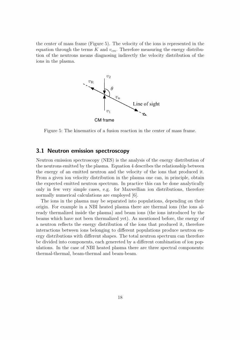
the center of mass frame (Figure 5). The velocity of the ions is represented in theequation through the terms K and vcm. Therefore measuring the energy distribu-tion of the neutrons means diagnosing indirectly the velocity distribution of theions in the plasma.

Figure 5: The kinematics of a fusion reaction in the center of mass frame.

3.1 Neutron emission spectroscopy

Neutron emission spectroscopy (NES) is the analysis of the energy distribution ofthe neutrons emitted by the plasma. Equation 4 describes the relationship betweenthe energy of an emitted neutron and the velocity of the ions that produced it.From a given ion velocity distribution in the plasma one can, in principle, obtainthe expected emitted neutron spectrum. In practice this can be done analyticallyonly in few very simple cases, e.g. for Maxwellian ion distributions, thereforenormally numerical calculations are employed [6].

The ions in the plasma may be separated into populations, depending on theirorigin. For example in a NBI heated plasma there are thermal ions (the ions al-ready thermalized inside the plasma) and beam ions (the ions introduced by thebeams which have not been thermalized yet). As mentioned before, the energy ofa neutron reflects the energy distribution of the ions that produced it, thereforeinteractions between ions belonging to different populations produce neutron en-ergy distributions with different shapes. The total neutron spectrum can thereforebe divided into components, each genereted by a different combination of ion pop-ulations. In the case of NBI heated plasma there are three spectral components:thermal-thermal, beam-thermal and beam-beam.

18

4 Neutron diagnostics

Neutrons are neutral, thus cannot be detected directly. The techniques used todetect neutrons rely on the conversion of the neutron into another particle, nor-mally a proton or a heavier ion, which is charged and can therefore be detectedfor example with a scintillator. In the case of energy measurements, the quantitydirectly detected by the spectrometer is not the neutron energy but som otherquantity that is related to it. For example in the time of flight technique the timeof flight of the neutron, which depends on the neutron energy, is what is actuallymeasured (more on the time of flight technique in section 4.3).

4.1 Quality of a neutron spectrometer

There are three instrumental properties that can be used to evaluate the quality ofa neutron spectrometer: the efficiency, the resolution and the shape of the responseof the spectrometer to neutrons.

The efficiency is simply the number of neutrons detected per number of incidentneutrons. A more efficient spectrometer gives more counting statistics, thereforecan allow either a finer time resolution or a more precise result in the same inte-gration time.

The resolution is the gaussian broadening of the spectra measured by the spec-trometer. A better resolution means that it is possible to distinguish between finerfeatures in the spectrum.

Finally the response function of the spectrometer is the spectrum produced bymonoenergetic neutrons. Ideally the best response would be a delta function,but the various processes involved in the conversion of the neutron energy into asecondary quantity introduce distortions to this ideal response. In general, if theresponse is closer to the ideal response, the analysis of the spectra is easier andmore precise.

4.2 The magnetic proton recoil technique

The magnetic proton recoil (MPR) technique is based on the conversion of neu-trons into protons via elastic scattering in a thin plastic foil and the subsequentmomentum separation of the recoil protons in a magnetic field.

An instrument based on this technique was installed by the Uppsala NeutronDiagnsotic Group at JET in 1996, inside the torus hall, and it was upgraded(MPRu) with digital acquisition boards in 2005 [8]. It was optimized for 14 MeVneutron measurements, but it can be used to measure 2.5 MeV neutrons too.

The main components of the MPRu spectrometer are shown in Figure 6. Theneutrons emitted by the plasma are formed into a ”neutron beam” by a collimator.

19

Figure 6: Components of the MPRu spectrometer.

They then enter the spectrometer’s vacuum chamber through a thin steel windowand impinge on a thin polythene foil, where they interact with protons via elasticscattering. Some of the protons are scattered in the forward direction (same di-rection of the incoming neutrons) and they pass through the proton collimantor.The relationship between neutron and proton energy is Ep = En cos2 θ, where θis the scattering angle in the laboratory system. Thus a proton scattered in theforward direction (θ = 90◦) has the same energy as the original neutron. Insidethe vacuum chamber two magnetic dipoles (D1 and D2) generate a magnetic fieldthat bends the trajectories of the protons towards the hodoscope, an array of plas-tic scintillation detectors. The bending radius of the protons inside the magneticfield is proportional to their velocity (r = mv/Bq), therefore different energies willcorrespond to different positions of impact on the hodoscope.

4.3 TOFOR

The Time Of Flight spectrometer Optimized for high Rate (TOFOR) was installedin the JET roof lab (above the tokamak) by the Uppsala group in 2005 [9]. It ismainly a 2.5 MeV spectrometer but it can also measure 14 MeV neutrons. Theprinciple of this spectrometer is the measurement of the time that it takes for

20

a neutron to cover a certain distance. This time is related to the energy of theneutron through the equation En = 2mnd

2/t2TOF , where d is the length of the flightpath and mn is the neutron mass.

Figure 7: Geometry of the TOFOR spectrometer. From [9]

The geometry of the TOFOR instrument is shown in Figure 7. The neutronsfrom the plasma are formed into a collimated “neutron beam” through a 2 meterlong aperture in the JET roof laboratory floor. Some of the incoming neutronsscatter in a first set of detectors (S1) which gives the start time. Some of thescattered neutron are subsequently detected in a second set of detectors (S2), thatgives the stop time. The S2 detectors are placed at an angle α 6= 0 with respectto the incoming neutron flux. The time of flight measured is therefore that of ascattered neutron with scattering angle α, which is related to the original neutronenergy by the equation:

E ′n = En cos2(α) =1

2mn

L2

t2tof. (5)

Noticing that L = 2r cos(α) the original neutron energy is simply obtained from:

En =1

2mn

r2

t2tof. (6)

21

4.4 Compact spectrometers

The spectrometers described so far are complex systems with a lot of components.Simpler and cheaper alternatives are the so-called compact spectrometers, suchas semiconductors (silicon and diamonds) and scintillators (organic and inorganicsolids and liquids). The problems with the compact spectrometers are that theirresolution is usually worse than for the optimized spectrometers and their responseto neutrons is not optimal for energy measurements (more in section 4.5).

4.4.1 Liquid scintillators

Liquid scintillators are usually made of organic compounds, therefore they containmainly hydrogen and carbon atoms [10]. At the energies of interest for DD fusionneutrons interact with hydrogen and carbon nuclei via elastic scattering. Otherreaction channels on carbon such as 12C(n, α)9Be, 12C(n, p)12B, and 12C(n, d)11Bbecome important only for neutron energies above 7 MeV.

The scattered proton is charged, therefore it is slown down by interacting withthe electrons in the material, which results in the excitation of molecular levels inthe scintillator. The consequent de-excitation produces light in the visible range,with a total intensity proportional to the energy deposited by the proton. Thelight produced from scattering on carbon is much less than that from hydrogen, soit contributes only to the low energy part of the measured spectrum [11]. The lightpulse produced can then be converted into a current pulse using a PhotomultiplierTube (PMT). The PMT is composed of a photo-cathode that converts photonsinto electrons through the photoelectric effect, and then a series of dynodes thatmultiplies the electrons, which are finally collected by an anode. The integral ofthe current pulse (total charge) is directly proportional to the intensity of the lightcollected by the photocathode, therefore it is proportional to the energy depositedin the scintillator. The spectrum constructed from the total charge of the eventsis referred to as pulse height spectrum (PHS).

There are several factors that contribute to the resolution of a detector basedon (liquid) scintillation and PMT:

1. spatial fluctuations in the light collection efficiency from different parts ofthe scintillation volume;

2. statistical variations in the number of photo-electrons produced and in themultiplication process in the PMT;

3. electrical noise on the signal.

These three effects are represented in the following empirical equation by theterms α, β, and γ respectively:

22

R(E) =FWHM(E)

E=

√α2 +

β2

E+γ2

E2, (7)

where R is the relative resolution, E is the deposited energy in MeVee (megaelectronvolt electron equivalent), and FWHM stands for full width at half maxi-mum.

Furthermore, if the pulses are recorded using a waveform digitizer, the resolutioncould be deteriorated if the bit resolution and sampling frequency of the digitizerare not chosen appropriately.

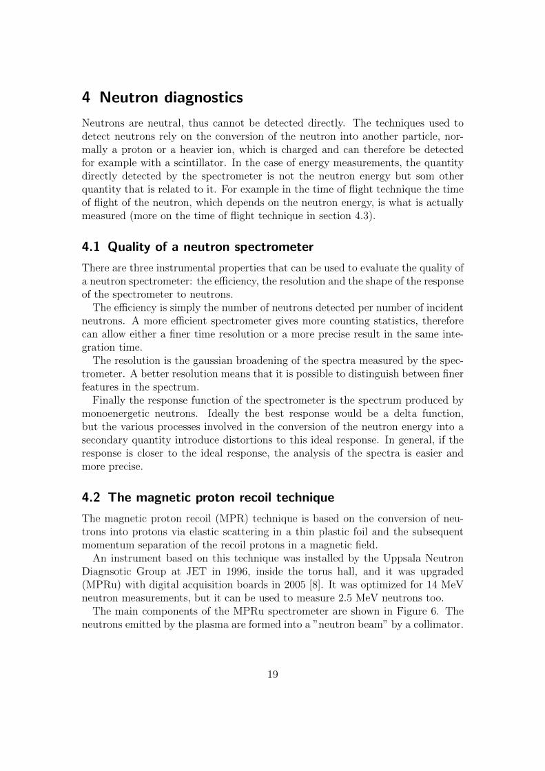
In a similar way to that for neutron detection, liquid scintillators can also detectgamma particles, the difference being that the gammas interact with electrons(mainly via Compton scattering) instead of protons. However some scintillatorsgive pulse shapes that depend on the interacting particle, which allows for theidentification of the type of particle that produced a specific pulse. The reason forthis is that different particles excite different molecular levels, which have slightlydifferent de-excitation times. This is reflected in the scintillation pulse shapes asshown in Figure 8: the tail of the neutron (proton) pulse shapes is longer thanthe one of the gamma (electron), a difference that can be exploited using varioustechniques to distinguish between neutron and gamma events.

Several organic liquid scintillator have been developed over the years, but theone that offers the best performance in terms of pulse shape discrimination is theNE213 type (a.k.a. BC-501A or EJ-301 depending on the manufacturer). TheNE213 compound is Xylene (C8H10) and it has a density of 0.874 g/mL [12].

140 160 180 200 220 240 260 280 300t [ns]

10-3

10-2

10-1

Amplitude [a.u.]

electronproton

Figure 8: Average proton (neutron) and electron (gamma) pulse shapes for aNE213 liquid scintillator.

23

It is important to know that the light emission from electron signals is linearlyproportional to the energy deposited in the detector (in the energy range interestingfor this work), but the same is not true for protons. The non-linearity makes theanalysis of neutron pulse height spectra more complicated than that of gammas.

4.5 Comparison between spectrometers

As mentioned before (section 4.1), the quality of a spectrometer can be judgedusing three properties. Tables 2 and 3 compare the efficiency and resolution ofthe optimized spectrometers (MPR and TOFOR) with the NE213 for 2.5 and 14MeV neutrons. Figure 9 shows their response to monoenergetic neutrons. Noticethat efficiency, resolution and response do not depend only on the technique butalso, to different degrees, on the specific design of the instrument. For example,the MPR employs a flexible system of conversion foils and proton apertures, whichmakes it possible to vary the performance within certain limits.

In general the resolution of the optimized spectrometers is better than theNE213, while for the efficiency it is the opposite. However one must be carefulwhen talking about efficiency, because the final counting statistics depends also onthe active area of the spectrometer (i.e. the area facing the plasma that can detectneutrons), the distance from the plasma and the dimensions of the collimator. Inaddition, practical aspects like gain stability, count rate capability, robustness etc.will also play a role in any practical implementation of a neutron spectrometer forfusion.

Regarding the neutron response functions, it is clear that the MPR and TOFORresponses are more suitable for spectroscopy because they are peaked, thus moresimilar to the ideal delta response than the NE213 response, which has a box-likeshape, extending up to a certain maximum.

Table 2: Efficiency and resolution of the MPR and NE213 for 14 MeV neutrons.

MPR NE213

Efficiency 0.51 – 11 · 10−6 ∼ 0.03

Resolution 1.95 – 4.24 % ∼ 4 %

Table 3: Efficiency and resolution of the TOFOR and NE213 for 2.5 MeV neutrons.

TOFOR NE213

Efficiency 0.01 ∼ 0.08

Resolution 7.4 % ∼ 12 %

24

Figure 9: Response of the MPR spectrometer to 12.6 MeV (black), 14.0 MeV (red),15.4 MeV (green) and 16.8 MeV (blue) neutrons (top); response of theTOFOR spectrometer to three neutron energies (middle); response ofthe NE213 spectrometer to 14 MeV neutrons (bottom).

25

26

5 The “Afterburner” installation

The MPRu spectrometer has a pre-prepared cavity in the back, before the beamdump, where different detectors can be tested. A NE213 liquid scintillator and adiamond detector [13] were installed in this cavity. The NE213 installation wasnamed “Afterburner”, since it measures neutrons after they have gone throughthe thin conversion foil, as well as the entrance and exit windows of the vacuumchamber of the MPRu. The original idea behind the installation was to allow neu-tron flux measurements with millisecond time resolution during DD operations,when the low efficiency of the MPRu prevents the time resolution of JET dis-charges. However in this work it was used to investigate the neutron spectroscopycapabilities of NE213 scintillators.

5.1 Detector specifications and assembly

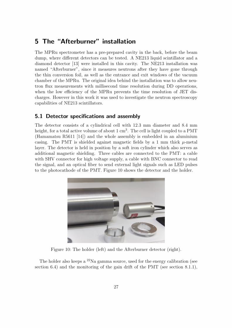
The detector consists of a cylindrical cell with 12.3 mm diameter and 8.4 mmheight, for a total active volume of about 1 cm3. The cell is light coupled to a PMT(Hamamatsu R5611 [14]) and the whole assembly is embedded in an aluminiumcasing. The PMT is shielded against magnetic fields by a 1 mm thick µ-metallayer. The detector is held in position by a soft iron cylinder which also serves asadditional magnetic shielding. Three cables are connected to the PMT: a cablewith SHV connector for high voltage supply, a cable with BNC connector to readthe signal, and an optical fiber to send external light signals such as LED pulsesto the photocathode of the PMT. Figure 10 shows the detector and the holder.

Figure 10: The holder (left) and the Afterburner detector (right).

The holder also keeps a 22Na gamma source, used for the energy calibration (seesection 6.4) and the monitoring of the gain drift of the PMT (see section 8.1.1),

27

in front of the detector.The full PMT pulses are recorded digitally using a SP Devices ADQ214 digitizer

(14 bit, 400 MSPS) [15] and stored on a local computer.

5.2 Line of sight and Field of view

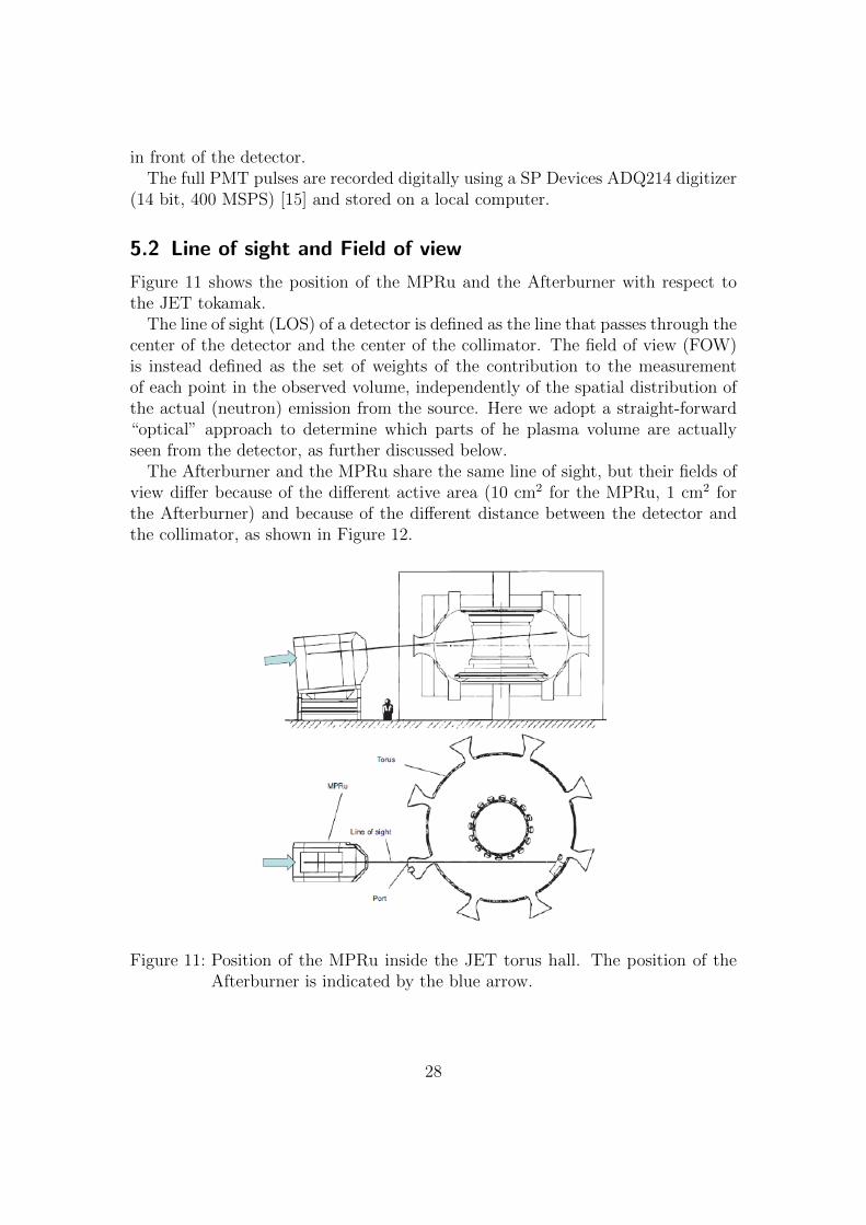
Figure 11 shows the position of the MPRu and the Afterburner with respect tothe JET tokamak.

The line of sight (LOS) of a detector is defined as the line that passes through thecenter of the detector and the center of the collimator. The field of view (FOW)is instead defined as the set of weights of the contribution to the measurementof each point in the observed volume, independently of the spatial distribution ofthe actual (neutron) emission from the source. Here we adopt a straight-forward“optical” approach to determine which parts of he plasma volume are actuallyseen from the detector, as further discussed below.

The Afterburner and the MPRu share the same line of sight, but their fields ofview differ because of the different active area (10 cm2 for the MPRu, 1 cm2 forthe Afterburner) and because of the different distance between the detector andthe collimator, as shown in Figure 12.

Figure 11: Position of the MPRu inside the JET torus hall. The position of theAfterburner is indicated by the blue arrow.

28

Most of the time the geometry of the FOW is complicated, so it is not practicalto calculate it analytically. Therefore a code named LINE 2 was developed tocompute the FOW numerically. It is an optical code: only geometrical effects areconsidered and no nuclear reactions are involved, therefore the hindering objectsare completely opaque and do not let any particle go through. In the input of thecode one defines the plasma volume, the detector position and dimensions, andthe limiting surfaces, i.e. all the surfaces that prevent the neutrons from reachingthe detector surface, such as the front of the collimator. The code divides theplasma volume in voxels and calculates the solid angle constituted by the detectoras seen from each of these voxels using numerical methods. The weight is then theproduct of the volume of the voxel times the solid angle.

R [m]

2 2.5 3 3.5 4

z [m

]

2−

1.5−

1−

0.5−

0

0.5

1

1.5

2

Afterburner

R [m]

2 2.5 3 3.5 4

z [m

]

2−

1.5−

1−

0.5−

0

0.5

1

1.5

2

MPRu

Figure 12: Poloidal projection of the FOW of the Afterburner (left) and the MPRu(right). The colour is proportional to the sum of the weights of thevoxels with coordinates (z,R).

29

30

6 Afterburner system characterization

6.1 Typical pulses

Figure 13 shows examples of pulse shapes recorded with the Afterburner. There arethree different processes that produce signals in the detector: gamma, neutron andLED induced events. Technical issues that still need to be investigated preventedthe collection of LED signals during the JET experiments used in this work.

0 50 100 150 200 250 300Sample

�200

0

200

400

600

800

1000

Ampl

itude

[a.u

.]

GammaNeutronLED

Figure 13: Typical Afterburner scintillation pulses produced by gammas (blue),neutrons (green) and LED signals(red).

6.2 Pulse shape discrimination

As shown in Figure 8, it is possible with NE213 scintillators to distinguish betweengamma and neutron induced signals, thanks to the difference in pulse shape. Thereare many practical ways of doing that, but the one that was chosen for the After-burner is the charge comparison method. It consists in integrating the pulses indifferent integration intervals, a short one and a long one, as shown in Figure 14.The integration over the long gate gives the total charge of the pulse (Qtot), whilethe integration over the short gate gives the short charge (Qshort). The factor usedfor pulse shape discrimination (PSD) is given by:

31

PSD =Qtot −Qshort

Qtot

. (8)

Figure 14: Integration gates used for pulse shape discrimination.

Since the neutrons have a more pronounced tail, the value of PSD for neutronevents will be higher than the one for gamma events. The recorded events canthen be collected in a 2D histogram, as shown in Figure 15, so that it is possiblethrough apporpriately chosen cuts to separate gamma and neutron events.

The quality of the PSD depends on the particle energy, being worse at lowenergies. It can be assessed by taking the 1D projection of the PSD histogramon the y axis, within a selected total charge interval, and then calculating thefollowing figure of merit (FOM):

FOM =∆PEAK

FWHMγ + FWHMn

, (9)

where FWHM stands for full width at half maximum and ∆PEAK is thedistance between the gamma and the neutron peaks, as illustrated in Figure 16.

The FOM values for some total charge intervals for Afterburner data from JETdischarge 86459 are shown in Table 4.

The FOM allows to compare the PSD performance of different detectors anddifferent PSD methods, but also allows to find the integration gates for the charge

32

Figure 15: 2D histogram for pulse shape discrimination.

Figure 16: Illustration of the components in the FOM calculation. 1D projectionof a slice of the PSD histogram on the y axis.

integration that give the best PSD. The values given in Table 4 were obtained withthe integration gates that give the highest FOM in the present study.

33

Table 4: FOM values for the Afterburner data from JPN 86459.

5k < Qtot < 10k 10k < Qtot < 15k 15k < Qtot < 20k

FOM 2.25 2.33 2.35

6.3 MCNPX model

In order to properly interpret the measured PHS it is necessary to know the de-tector response to both gammas and neutrons. The response can be computedby numerical simulations using a MCNPX model of the detector [16]. Figure 17shows the geometry of the model, which includes the whole MPRu spectrometerwith its concrete shielding.

Figure 17: Geometry of the MCNPX model of the MPRu and Afterburner;overview (left) and close view on the Afterburner (right).

The response to gammas is calculated only at the energies of emission of the 22Nagamma source: 511 keV and 1275 keV. The two energies are simulated separately.In the simulation the gamma particles are emitted isotropically from the positionwhere the source is located. The energy deposited in the scintillator is recordedin a histogram which represents the response of the detector. Figure 18 shows thecalculated response to the two gamma energies.

For the response to neutrons the process is similar, but since the distributionof energies of the neutrons that are expected to impinge on the detecor are notknown a priori and change depending on the plasma conditions, a response matrixis built simulating monoenergetic neutrons from 1 to 7 MeV with 50 keV steps.The neutrons are generated uniformly from a disk source placed at the front ofthe neutron collimator, with direction parallel to the axis of the collimator. Theradius of the disk source is slightly bigger than the radius of the collimator entrance.

34

0.0 0.2 0.4 0.6 0.8 1.0 1.2 1.4Energy [MeVee]

0.0000

0.0001

0.0002

0.0003

0.0004

0.0005

0.0006

0.0007Co

unts

per

sim

ulat

ed p

artic

le

511 keV1275 keV

Figure 18: Response of the Afterburner detector to the gamma energies emittedby a 22Na source calculated with MCNPX.

Each of the rows of the matrix is a PHS obtained from a monoenergetic neutron.This way the expected PHS from a certain neutron spectrum can be obtained bymultiplying the neutron spectrum with the response matrix:

Mj = NRMi,j · Si, (10)

where M is the estimated PHS, NRM is the neutron response matrix, S isthe neutron spectrum, the subscript j represents the light yield i represents theneutron energy.

The simulation of the neutron response is more complicated because of the factthat the proton light yield of NE213 scintillators is not linear (see section 4.4.1).MCNPX allows the user to introduce a non-linear light yield function in order toget the proper intensity of the scintillation light in the detector. The scintillationlight from scattering on carbon is not included in the calculation. However this isnot a problem if the analysis of the PHS is performed with a energy threshold highenough, since the intensity of the light produced by recoil carbon is low comparedto that produced by protons. For neutron energies above 7 MeV one needs toinclude the effect of other, inelastic, reactions on carbon in the calculation, as

35

explained in section 4.4.1.Figure 19 shows the calculated response of the Afterburner to some neutron

energies.

0 1 2 3 4 5Energy [MeVee]

0.0000

0.0002

0.0004

0.0006

0.0008

0.0010

0.0012

0.0014

0.0016

0.0018

Coun

ts p

er s

imul

ated

par

ticle

2.0 MeV4.0 MeV6.0 MeV

Figure 19: Response of the Afterburner detector to monoenergetic neutrons of 2(blue) 4 (green) and 6 (ref) MeV calculated with MCNPX.

6.4 Gamma and neutron calibration

The MCNPX simulation does not include the resolution of the detecor, nor the con-version factor between light output, which is given in electronvolt electron equiva-lent (eVee) units, and the total charge obtained in the integration of the measuredpulses. The resolution can be added to the simulated response by substitutingeach point with a gaussian with FWHM given by equation 7. The relationshipbetween eVee and total charge is linear (in the energy region of interest), thus canbe described by the simple equation:

E[keV ee] = k ·Qtot +m. (11)

The three resolution parameters α, β, γ of equation 7 and the two calibrationparameters k and m are not known a priori, but they can be obtained from a

36

fit of the well known 22Na gamma spectrum measured with the detector. Asmentioned before, the 22Na source produces 2 gamma lines. Each of them carriesinformation about the calibration (through the position of the Compton edge)and the resolution (through the broadening of the Compton edge), hence thereare 4 “information points” in the 22Na spectrum. To overcome the problem thatthere are only 4 points for 5 fitting parameters, the PHS of neutrons emitted fromohmically heated plasmas can be used as a known spectrum for calibration. It canbe demonstrated that the neutron spectrum from ohmic plasmas is a Gaussiandistribution with broadening proportional to the square root of the ion temperature[7]. At JET the ion temperature for ohmic plasma discharges is about 2 keV.

With the ohmic spectrum we are adding two extra “information points” (Theposition of the edge of the spectrum and its broadening), giving 6 in total for 5fitting parameters. We can therefore add a sixth parameter that we call kn. It is aparameter that we apply to the neutron response matrix only, as a multiplicationfactor to the light output axis of the matrix. For instance, if kn = 0.5 the columnin the response matrix that originally corresponded to 1 MeVee will become 0.5MeVee. The reason for this addition is the fact that there is no measurement ofthe proton light yield of the detector, therefore a standard light yield function fromliterature needs to be assumed for the MCNPX calculation of the response. Thekn factor introduces a correction to this assumption.

The evaluation of the parameters is done iteratively with the following steps:

1. fit gamma PHS with α, γ, k, m as free parameters (β fixed);

2. fit neutron PHS with kn, β as free parameters (α, γ, k, m fixed).

After some iterations the value of the parameters converges. In this study, theparameter α converges to zero, probably because the small dimensions of the de-tector make the light collection fairly uniform. This simplifies the calibration pro-cesses, since it is possible to assume α = 0 and the gamma and neutron calibrationcan be performed separately without iteration.

Figure 20 shows a fit of the 22Na gamma PHS and Figure 21 shows a fit of theohmic neutron PHS. The ohmic spectrum includes two components, the directspectrum and the backscatter. For the direct spectrum an ion temperature of 2keV was assumed. The evaluation of the backscatter component will be describedin section 8.2.1. The ohmic PHS is the sum of the ohmic part of about 650 JETdischarges from campaign C33 (from JPN 84743 to JPN 85396).

The results of the calibration for the data from the JET experimental campaignC33 are shown in Table 5.

37

channel20 30 40 50 60

counts/ch

2000

4000

6000

8000

10000

12000

14000

16000

18000

20000

/fusion/afterburner/C33/Analyzed/gamma_2.dat

Figure 20: Example of a fit of a 22Na gamma spectrum measured with the Af-terburner. The points are the measured data, The black dashed lineis the 511 keV component, the red dash-dotted line is the 1275 keVcomponent and the the blue line is the sum of the two.

Table 5: Resolution and calibration parameters for the data from JET campaign C33.

Parameter Value Uncertainty

α 0 N.A.

β 8.76 0.26

γ 4.53 0.20

k[keV ee/channel] 16.939 0.010

m[keV ee] 17.58 0.22

kn 0.967 0.002

38

channel

30 32 34 36 38 40 42 44 46 48 50 52

co

un

ts/c

h

200

400

600

800

1000

Afterburner ohmic data

Figure 21: Fit of the ohmic data from campaign C33. The total spectrum (bluesolid) is composed of two components: the direct spectrum (red dashed)and the backscatter (black dot-dashed).

39

40

7 Dacsim - Data acquisition chain simulation (PaperI)

Understanding the effect of the acquisition chain (PMT, cable, digitizer) on theconversion of scintillation light into an electric signal can help in the evaluationof the performance of a system. The Dacsim (Data acquisition chain simulation)code was developed for this purpose [17] [18].

7.1 The code

The starting assumption is that each event deposits a certain amount of energy(in MeVee) in the scintillator. The energy distribution of the events can be chosenarbitrarily with an input file.

The energy is converted into a number of photo-electrons which is Poisson dis-tributed, with the average number being proportional to the deposited energy.The proportionality factor is the product of the energy conversion factor (pho-tons/MeVee), the quantum efficiency of the photocathode, and the light collectionefficiency. The quantum efficiency and the light collection are assumed to be con-stant in space, while in reality they can change depending on the position of energydeposition. The photo-electrons are then spread in time according to a exponen-tial decay function composed of three decay times, which correspond to differentmoleculare excitation levels. As explained in section 4.4.1 electrons and protonsexcite different molecular levels, therefore their signal’s decay times are different,and this is considered in the code.

The multiplication in the PMT is a Poisson process in which the variance isdominated by the first dynode in the chain [10]. This is implemented in thecode by producing a multiplication factor for each of the photo-electrons which isproportional to the overall gain but has a relative variance given by:

σ2gain

gain=

1

δ − 1, (12)

where δ is the multiplication factor of a single dynode. The signal is thenconvolved with a Gaussian that simulates the PMT time response.

The cable filters low frequencies in the signal, and the level of attenuation de-pends on the type and the length of the cable. In the code the cable is modeledas a simple low-pass filter for which it is possible to select the cut-off frequency.Electric noise is also added as random Gaussian oscillations on the signal. Theintensity of the noise can be chosen in the input file.

Finally the digitizer simply samples the signal with a given sampling frequencyand resolution.

41

The code can also simulate pile-up, by generating a series of random triggertime intervals according to the count rate, which can be chosen in the input file.When the time interval is shorter than the total pulse length, the correspondingevents are added up, simulating a pile-up event. The addition is performed beforethe PMT response is added.

7.2 Examples

An example of the average pulses generated by the code compared to pulses mea-sured by the Afterburner is shown in Figure 22.

20 40 60 80 100 120 140t [samples]

0.00

0.02

0.04

0.06

0.08

0.10

0.12

0.14

Amplitude [a.u.]

realsimulated

20 40 60 80 100 120 140t [samples]

0.00

0.02

0.04

0.06

0.08

0.10

Amplitude [a.u.]

realsimulated

Figure 22: Comparison between the average gamma (left) and neutron (right)pulses from the Afterburner (blue dots) and from the Dacsim code (redline). The code input was set-up to obtain a good match with the realpulses.

One can use the code for example to study the effect of the data acquisitionchain on the pulse shape discrimination. Figure 23 shows simulated PSD plotswithout and with pile-up.

The code was used to evaluate the goodness of the pile-up rejection method usedfor the Afterburner. The results of the evaluation are presented in section 8.1.2.

42

0 10000 20000 30000 40000 50000 60000 70000 80000Total charge [a.u.]

0.0

0.1

0.2

0.3

0.4

0.5

0.6

0.7

0.8PSD fact

or

PSD of simulation without pile-up

5

10

15

20

25

30

35

40

0 10000 20000 30000 40000 50000 60000 70000 80000Total charge [a.u.]

0.0

0.1

0.2

0.3

0.4

0.5

0.6

0.7

0.8

PSD fact

or

PSD of simulation with pile-up

4

8

12

16

20

24

28

32

36

Figure 23: Pulse shape discrimination plots of the simulated pulses without pile-up(top) and with pile-up (bottom).

43

44

8 Data analysis

8.1 Data processing

Before the actual spectroscopic analysis, the data need to be treated to accountfor two effects: gain drift and pile-up.

8.1.1 Gain drift

Gain drifts are changes in the gain of the PM tube. It is convenient to classify gaindrifts according to the time scale during which they occur: long term (∼days) andshort term (∼milliseconds).

The long term gain drifts are caused by temperature changes and deterioration ofthe tube. A reliable way to measure long term gain drifts is to perform periodicalmeasurements of the gamma spectrum from a calibration source and from thatcalculate the calibration parameters (as shown in section 6.4). This has been donefor the Afterburner system on a daily basis during the JET campaigns.

The calibration parameter that is related to the gain is the coefficient k. Figure24 shows the daily variation of this coefficient during the C33 campaign at JET.It can be noticed that there was a clear deterioration of the gain in the first halfof the experimental period, reflected in the plot as an increase in the coefficient k.

Data set0 5 10 15 20 25 30 35 40 45

k [

ke

Ve

e/c

ha

nn

el]

17.2

17.3

17.4

17.5

17.6

17.7

Calibration slopeCalibration slope

Figure 24: Variation of the calibration parameter k during the C33 campaign atJET. The parameter is inversly proportional to the gain of the PMT.

45

The correction procedure is straightforward. First one chooses a reference day.Then the total charge of any other day is rescaled to restore the reference calibra-tion, using the formula:

Q′tot =Qtot · k + (m−mref )

kref. (13)

The short term gain drifts are caused by high count rates, which produce acurrent in the PMT that is comparable to the current in the voltage divider circuit.The gain drift is obtained from the formula [19]:

∆G

G= α

N

N + 1

IaIp, (14)

where G is the gain, N is the number of dynode stages in the PMT, Ia is theanode current. Ip is the current flowing in the voltage divider circuit of the PMT,and α is a constant.

Equation 14 implies that the gain increases linearly with the anode current,which in turn is linearly proportional to the count rate in the detector. Howeverwhen the ratio Ia/Ip approaches 1, the equation does not hold since the anodecurrent is so high that space charge starts influencing the electron trajectories,making the collection efficiency drop drastically. Consequently the gain decreasesquickly too.

One way to monitor the short term gain drift is to shine a LED signal into thePMT and monitor the variations in its total charge. If the LED generator is stableenough the only factor affecting the total charge is the gain of the PMT.

The Afterburner is equipped with a LED generator, but technical issues pre-vented the collection of LED signals during the period of JET campaigns used inthis work. In order to obtain an estimate of the gain correction required, LEDdata from another experiment was used, namely from the NE213 detectors of theMAST neutron camera [20]. These detectors are also NE213 connected to exactlythe same kind of PMT as the Afterburner, and with a similar high voltage levelapplied. Furthermore the average amplitude of the pulses recorded by the MASTdetectors is similar to the average amplitude of the Afterburner pulses. Thereforeit was possible to use the gain variation as function of count rate in the MASTdetectors as an estimate of the gain variation versus count rate in the Afterburner.

The relative variaiton of the LED total charge vs count rate in the MASTdetectors is shown in Figure 25. The count rate in the Afterburner during JETcampaign C33 did not exceed 100 kHz, therefore the maximum gain variation isexpected to stay within a few percent.

46

0 100000 200000 300000 400000 500000 600000 700000 800000Count rate [Hz]

−0.10

−0.05

0.00

0.05

0.10

0.15

0.20

0.25

0.30

∆QLED/Q

LED,ref

Gain variation vs count rate

Figure 25: Relative variation of the LED total charge vs count rate in the MASTdetectors.

8.1.2 Pile-up rejection

Pile-up occurs when two or more events happen in a time interval shorter thanthe length of a single event. If not treated properly, pile-up can lead to errors inthe evaluation of the total charge of the events.

In this work pile-up events were rejected applying cuts in the PSD plot as shownin Figure 26. This simple method was proven to be applicable using the simulationcode described in chapter 7. The code was set up to resemble the experimentalconditions of the Afterburner in terms of pulse shapes, energy distribution of theevents and count rate. Two simulations, one with and one without pile-up, werecompared (Figure 27). A Kolmogorov-Smirnov test of the two distributions (withQtot > 10000) gave 81% probability of the two data sets being sampled from thesame distribution, therefore we can safely assume that the two distributions areequivalent.

8.2 Analysis of the neutron pulse height spectra

The strategy for the NES analysis is to model the ion distribution, use it to calcu-late the neutron emission, fold the resulting neutron spectrum with the responseof the instrument (equation 10) and compare the final result with the experimen-tal measurement. In some cases the modeled neutron spectrum depends on some

47

Figure 26: PSD plot for JPN 86463. The cuts applied are shown in red. The eventsabove the neutron cluster are rejected as pile-up events.

parameters that can be fitted to match the data. This analysis strategy is usuallyreferred to as forward folding or forward fitting.

As explained in section 3.1 the neutron spectrum can be divided into spectralcomponents. These components can be kept separated in the analysis and theycan then be fitted independently to the data. This way the intensities of thecomponents can be fitting parameters.

An extra spectral component which is present for any plasma condition is thebackscatter component. Backscattered neutrons are neutrons that are reflected bythe tokamak wall opposite to the spectrometer as seen in the FOW of the spec-trometer. Their energy distribution depends on the original energy distribution ofthe neutrons and on the wall materials. To estimate the backscatter componenta backscatter matrix is generated with MCNPX simulations with monoenergeticneutrons. This matrix is an actual response matrix: given the direct neutron spec-trum emitted by the plasma one can obtain the expected backscatter spectrum atthe detector position by folding the direct spectrum with the backscatter matrix,similarly to what is done in equation 10.

The statistical error in the estimate of the fitting parameters is obtained by sam-pling randomly the chi-square probability space independently for each of them.The contribution of the calibration parameters to the systematic uncertainty isestimated by varying separately each of them by ±σ and performing the fit again.

48

The difference between the values of the fitted parameters with unchanged andchanged calibration parameter is the contribution of that calibration parameter tothe uncertainty.

8.2.1 Thermal fraction estimate (Paper II)

The ratio between the intensity of the thermal component of the neutron spectrumand the total direct spectrum is referred to as the thermal fraction and it is a wayto evaluate how much the plasma relies on external heating.

In the NE213 PHS the difference between a purely thermal (ohmic) plasma anda plasma with NBI heating is not very pronounced, but it is clearly visible (Figure28). The tail in the NBI heated spectrum is slightly more pronounced because ofthe presence of a beam-thermal component, a fact that points to the possibility toseparate the spectral components.

Some JET pulses from campaigns C31 and C32 were selected to study the pos-sibility to use NE213 detectors in the thermal fraction estimate. The criteria forpulse and time slice selection were:

1. NBI is the only additional heating in the pulse;

0 10000 20000 30000 40000 50000 60000 70000 80000Total charge [a.u.]

10-6

10-5

10-4

Norm

aliz

ed counts

Normalized neutron spectra

no pile-uppile-up

Figure 27: Comparison of the simulated neutron PHS without pile-up (blue solid)and with pile-up after the applications of the same cuts as in the realdata (red dashed).

49

channel0 10 20 30 40 50 60 70 80 90

counts

/ch

0

0.005

0.01

0.015

0.02

0.025

0.03

0.035

0.04

0.045

Spectrum

Entries 123119

Mean 27.92

RMS 10.15

Ohmic vs NBI heated spectrum

Figure 28: Normalized neutron PHS measured by the Afterburner during ohmicJET discharges (black) and during NBI heated discharges (red). TheNBI heated spectrum has a slightly longer tail.

2. The relevant plasma parameters (electron temperature, electron density, neu-tron yield, Zeff

1) measured by other JET official diagnostics in the selectedtime interval are stable;

3. high electron density (ne ∼ 1020m−3) so that the beam-beam component isnegligible, and Ti ≈ Te can be assumed.

Furthermore the selected discharges needed to cover a relatively wide range ofthermal fraction values.

The ion velocity distributions for the pulses were obtained from simulationswith the TRANSP code [21]. The components of the neutron spectrum in theAfterburner FOW were then obtained applying the ControlRoom code [22] to thedistributions from TRANSP.

The free parameters in the fit were the intensities of the components and the iontemperature, for which the measurement of the electron temperature was set as aBayesian prior (assuming a relative uncertainty of 10% on the Te measurement).

For the analysis of the PHS a first fit of the data without the backscatter compo-nent is performed; then the result of this fit is folded with the backscatter matrix

1The effective ion charge is defined as Zeff =∑

i njZ2j∑

i njZj, where j denotes the ion species in the

plasma, n is the density, Z is the charge.

50

to obtain the backscatter component; finally the backscatter component is addedto the spectrum and a new fit is performed.

It is very important to consider the fact that the neutron spectrum and thebackscatter matrix depend on the FOW of the instrument. To take that intoaccount the result of the LINE 2 code is included as an input of the code thatperforms the calculation of the spectral component.

Figure 29 shows the time evolution of the most important parameters of JETpulse number 84866. Figure 30 shows the results of the fit of pulse 84866 in thetime interval t = 55− 58s for the Afterburner and TOFOR. The Afterburner datastart from channel 30 for many reasons: avoiding the modeling of the threshold,avoiding the region where the PSD is not so good, avoiding the region where thelight yield from carbon needs to be included in the calculation of the responsematrix. The data are fitted only up to channel 60 to avoid the inclusion of emptybins.

Figure 29: Time evolution of the most important parameters for JPN 84866. Fromtop: total neutron yield; total NBI power; electron density in the core;Zeff ; electron temperature in the core.

The estimates of the thermal fraction for the selected pulses are summarized inTable 6 together with the estimated statistical and systematic errors.

Figure 31 shows the comparison between the Afterburner and the TOFOR ther-mal fraction estimate. In the plot the correlation between the two is clear; however

51

channel

30 35 40 45 50 55

counts

/ch

1

10

210

310

84866 55.0­58.0 s

[ns]TOF

t50 55 60 65 70 75 80

counts

/ b

in

1

10

210

JET #84866 @ t=55.0­58 s

total

THN

NBI

scatt

Figure 30: Fit of the Afterburner (left) and TOFOR (right) data for JPN 84866.The only additional heating was NBI. The components of the neu-tron spectrum are: thermal-thermal (THN), beam-thermal (NBI) andbackscatter (scatt).

it is also clear that there is a bias in the comparison, since the Afterburner esti-mate is systematically higher than the TOFOR estimate. This might be explainedby the fact that plasma rotation, which would affect the neutron spectrum alongthe Afterburner LOS but not the one along the TOFOR LOS, was not included inthe neutron emission model. It should also be noted that the uncertainties in theresults from the Afterburner are 4 to 7 times higher than those from TOFOR.

Table 6: Results of the thermal fraction analysis. The columns, from left to right, are:JET pulse number; selected time interval in the JET pulse; TOFOR estimateof the thermal fraction; Afterburner estimate of the thermal fraction; statisticaluncertainty on the Afterburner estimate; negative systematic uncertainty onthe Afterburner estimate; positive systematic uncertainty on the Afterburnerestimate.

Discharge # ∆t (s) IthItot

(TOFOR) IthItot

(Afterburner) σstat σ−sys σ+sys

84866 55.0− 58.0 0.087± 0.012 0.227 0.025 0.030 0.045

84886 50.5− 52.5 0.247± 0.017 0.378 0.028 0.036 0.048

84889 52.0− 55.0 0.273± 0.014 0.419 0.023 0.031 0.036

84976 49.0− 51.0 0.196± 0.016 0.285 0.029 0.031 0.081

84976 53.6− 55.6 0.0 0.131 0.050 0.030 0.019

85387 57.0− 59.0 0.136± 0.013 0.161 0.030 0.006 0.072

52

Figure 31: Comparison between the Afterburner and the TOFOR estimates of thethermal fraction. The red solid line represents the best linear fit; theblue dashed line represents the ideal 1 to 1 relationship. Reprinted withpermission from Rev. Sci. Instrum. 85, 11E123 (2014). Copyright2014, AIP Publishing LLC.

8.2.2 Third harmonic radio-frequency heating analysis (Paper III)

Third harmonic radio-frequency (RF) heating is a type of ICR heating that, as thename says, exploits the resonace of the 3rd harmonic of the ion cyclotron frequency.This heating scheme, used in combination with NBI heating, produces very ener-getic fuel ions, and consequently the neutron spectrum presents a distinctive highenergy tail, reflecting the high energy tail in the ion distribution. The maximumenergy in the ion distribution is inversly proportional to the electron density [23].

The effect can be clearly seen in the NE213 spectra as shown in Figure 32, whichalso shows that the endpoint of the tail of the spectrum is sensitive to changes inthe electron density.

Since the interest here is mainly in the high energy tail, the influence on thePHS from triton burn-up neutrons must be considered. Because of the box-likeshape of the neutron response of the NE213 (Figure 19) the 14 MeV neutrons fromtriton burn-up affect the PHS down to very low energies. The number of countsfrom TBN is not high, but it can affect the endpoint of the tail of the spectrum,as shown in Figure 33.

The TBN contribution was removed assuming that it produces a flat distributionof events over the entire energy range up to about 4 MeVee. This assumption is notgood for low energies, but it holds in the range of energies where we perform thedata analysis (above ≈ 1 MeVee). The estimate of the height of this contribution

53

Energy [MeVee]0.2 0.4 0.6 0.8 1 1.2 1.4 1.6 1.8 2

Norm

aliz

ed c

ounts

­310

­210

­110

RF tails

86463 48­49s (no RF)

86463 51­52s (RF, low density)

86464 51­52s (RF, high density)

Figure 32: Afterburner neutron PHS for JET discharges with NBI heating only(solid black), with NBI+RF heating and low electron density (dash-dotted red) and with NBI+RF heating and high electron density(dashed blue).

Energy [MeVee]0 0.5 1 1.5 2 2.5 3 3.5 4 4.5 5

Counts

1

10

210

310

410

JPN 86459 50.5­52.1s

Figure 33: Afterburner neutron PHS for JPN 86459. The plateau from 2 to 4.5MeVee comes from TBN signals.

was given by the average counts in the PHS bins from 2.4 to 4 MeVee.Figure 34 shows the comparison between data (after the triton burn-up correc-

tion) and the modeled PHS for JET discharges 86459 and 86464. The model used

54

for the ion distribution is based on a 1D Fokker-Plank model described in [23, 24].The parameters of the model are optimized to fit the data from TOFOR.

60 70 80 90 100 110 120channel

100

101

102

103

counts/bin

NE213 data JPN 86459 50.5-52.1 s

verbinskihawkeseddata

60 70 80 90 100 110 120channel

100

101

102

103

counts/bin

NE213 data JPN 86464 51.0-53.0 s

verbinskihawkeseddata

Figure 34: Comparison between the modeled and the measured neutron PHS forJPN 86459 and 86464.

Fig. 34 also shows results from an assessment of the impact of using differentproton light yield functions from literature in the analysis. Three different responsematrices were produce using different light yield functions [11, 25, 26] and thenused separately for the analysis. The chi-square values from the comparisons aresummarized in Table 7. The overall agreement is good, but in both discharges itseems that the model underestimates the endpoint of the spectrum. This mightbe caused by the simplified assumptions used in the modeling of the fuel iondistribution functions in references [23, 24]. In this modeling the pitch angles ofthe ions (i.e. the angle between the velocity of the ion and the magnetic field) areevenly distributed between 80 and 100 degrees. This assumption does not affectmuch the resulting spectrum along the TOFOR line of sight, while the spectrumalong the Afterburner line of sight is very sensitive to changes in the pitch angledistribution. This indicated that more realistic and detailed models of the fuel ionvelocity distribitions should be used in future studies of these experiments.

Table 7: reduced chi-square values obtained in the comparison between modeledand measured neutron PHS for JET discharges 86459 and 86464.

Hawkes ED Verbinski

86459 1.95 1.68 2.15

86464 1.67 1.63 1.85

55

56

9 Conclusions

The objective of this work is to assess the potential and the limits of the use ofNE213 liquid scintillators as neutron spectrometers for fusion plasmas. A NE213liquid scintillator, the Afterburner, was installed at JET on the same line of sightof the MPRu spectrometer and used to collect data during the JET experimentalcampaigns to attempt neutron emission spectroscopy analysis.

The understanding of the spectroscopy capabilities of the detector can be achievedonly after a proper characterization of the response of the detector, which here wasobtained by combining simulations of the system with MCNPX and real measure-ments. The calibration measurements included data both from a 22Na gammasource and from JET plasma discharges with ohmic heating only.

The Dacsim code was developed to simulate detector pulses including the effectof the components of the data acquisiton chain. The code was used to validate thepile-up rejection method used for the data analysis.

Neutron pulse height spectra from NBI heated plasmas were analysed and thethermal fraction in the neutron emission was estimated. The results were comparedwith the thermal fractions obtained with the TOFOR spectrometer. The estimatesfrom the two instruments showed a clear correlation. The uncertainty on theAfterburner estimates were 4 to 7 times higher than for TOFOR. A systematicbias in the comparison is also present and might be explained by the fact that theinstruments have different lines of sight.

The high energy tail of the neutron pulse height spectra from third harmonicRF heated plasmas were compared to the modeled PHS, which was optimizedto fit the TOFOR data. The comparison was good but the model gives a slightunderestimate of the endpoint of the PHS. This might again be explained by thefact that the different lines of sight are less or more sensitive to different parametersin the model.

The experience gained in this study permits to conclude that NE213 liquidscintillators can provide valuable spectroscopic information, but the quality ofthe results is far from the more complex instruments such as TOFOR, which areotpimized for neutron spectroscopy.

57

58

Acknowledgments

Many people deserve to be thanked for many reasons.Goran, thanks for beign such a wise mentor. Thanks Erik and Carl for all

the scientific input you give to my work. Thanks Jacob and Sean for providingconstant supervision, despite not being officially listed as supervisors.

Thanks to the other collegues of the Fusion group (present and past): Anders,Iwona, Marco, Mateusz, Matthias, Natalia, Siri. All of you make/made my workingtime a real pleasure.

Thanks to all the collegues of the Applied Nuclear Physics division for the nicefika and lunch discussion.

A special thanks goes to Andrea, Henrik, Bill, Katerina, Nico, Maaike, Tuur:thank you for your beautiful friendship.

Grazie alla mia famiglia per sostenermi a distanza con tutto l’affetto possibile.

Gracias Cristina por todo el amor que pones en mi vida.

59

60

References

[1] J. Onega and G. Van Oost, Energy for future centuries:prospects for fusionpower as a future energy source, Transactions of Fusion Science and Technol-ogy 53 (2008) 3.

[2] D. H. Crandall, The scientific status of fusion, Nucl. Instrum. Methods Phys.Res. B 42 (1989) 409.

[3] F. F. Chen, Introduction to plasma physics and controlled fusion, Volume 1:Plasma physics, 2nd edition, Plenum Press, New York, 1984.

[4] J. Wesson, Tokamaks, 2nd edition, Clarendon Press, Oxford, 1997.

[5] M. A. Pick and Jet Team, The technological achievements and experience atJET, Fusion Eng. Des. 46 (1999) 291.

[6] B. Wolle, Tokamak plasma diagnostics based on measured neutron signals,Physics Reports 312 (1999) 1.

[7] H. Brysk, Fusion neutron energies and spectra, Plasma Phys. 15 (1973) 611.

[8] E. Andersson Sunden et al., The thin-foil magnetic proton recoil neutron spec-trometer MPRu at JET, Nucl. Instrum. Methods Phys. Res. A 610 (2009) 682.

[9] M. Gatu Johnson et al., The 2.5-MeV neutron time-of-flight spectrometerTOFOR for experiments at JET, Nucl. Instrum. Methods Phys. Res. A 591(2008) 417.

[10] G.F. Knoll, Radiation detection and measurements, John Wiley and Sons,Inc., New York 2000.

[11] V. V. Verbinski et al., Calibration of an organic scintillator for neutron spec-trometry, Nucl. Instr. and Meth. 65 (1968) 8.

[12] http://www.eljentechnology.com/index.php/products/liquid-scintillators/71-ej-301 (Accessed 21 April 2015).

[13] C. Cazzaniga et al., Single crystal diamond detector measurements ofdeuterium-deuterium and deuterium-tritium neutrons in Joint EuropeanTorus fusion plasmas, Rev. Sci. Instrum. 85 (2014) 043506.

[14] http://pdf.datasheetcatalog.com/datasheet/hamamatsu/R5611-01.pdf (Ac-cessed 21 April 2015).

[15] http://spdevices.com/index.php/adq214 (Accessed 21 April 2015).

61

[16] See http://mcnpx.lanl.gov/ for MCNPX code (Accessed 21 April 2015).

[17] Code hosted on https://github.com/FedericoBinda/dacsim (Accessed 21April 2015).

[18] Documentation of the code hosted on https://dacsim.readthedocs.org (Ac-cessed 21 April 2015).

[19] S. O. Flyckt and C. Marmonier Photomultiplier Tubes: Principles and Appli-cations , Photonis, Brive, France (2002).

[20] M. Cecconello et al., The 2.5 MeV neutron flux monitor for MAST, Nucl.Instrum. Methods Phys. Res. A 753 (2014) 72.

[21] J. P. H. E. Ongena et al., Numerical transport codes, Trans. Fusion Sci. Tech-nol. 61 2T (2012) 180.

[22] L. Ballabio. Calculation and Measurement of the Neutron Emission Spectrumdue to Thermonuclear and Higher-Order Reactions in Tokamak Plasmas, PhDthesis, Uppsala University (2003).

[23] C. Hellesen et al., Fast-ion distributions from third harmonic ICRF heatingstudied with neutron emission spectroscopy , Nucl. Fusion 53 (2013) 113009.

[24] T. H. Stix, Fast-wave heating of a two-component plasma, Nucl. Fusion 15(1975) 737.

[25] N. P. Hawkes et al., Measurements of the proton light output function of theorganic liquid scintillator NE213 in several detectors, Nucl. Instrum. MethodsPhys. Res. A 476 (2002) 190.

[26] G. Dietze and H. Klein, NRESP4 and NEFF4: Monte Carlo Codes for the Cal-culation of Neutron Response Functions and Detection Efficiencies for NE213Scintillation Detectors, PTB Report PTB-ND-22, 1982, ISSN 0572-7170.

62