Neurale netwerken : kennis van nu, mogelijkheden vanmorgen : symposium, 3 april 1997, Technische UniversiteitEindhovenCitation for published version (APA):Institute of Electrical and Electronics Engineers (IEEE). Student Branch Eindhoven (SBE) (1997). Neuralenetwerken : kennis van nu, mogelijkheden van morgen : symposium, 3 april 1997, Technische UniversiteitEindhoven. Eindhoven: Technische Universiteit Eindhoven.

Document status and date:Gepubliceerd: 01/01/1997

Document Version:Uitgevers PDF, ook bekend als Version of Record

Please check the document version of this publication:

• A submitted manuscript is the version of the article upon submission and before peer-review. There can beimportant differences between the submitted version and the official published version of record. Peopleinterested in the research are advised to contact the author for the final version of the publication, or visit theDOI to the publisher's website.• The final author version and the galley proof are versions of the publication after peer review.• The final published version features the final layout of the paper including the volume, issue and pagenumbers.Link to publication

General rightsCopyright and moral rights for the publications made accessible in the public portal are retained by the authors and/or other copyright ownersand it is a condition of accessing publications that users recognise and abide by the legal requirements associated with these rights.

• Users may download and print one copy of any publication from the public portal for the purpose of private study or research. • You may not further distribute the material or use it for any profit-making activity or commercial gain • You may freely distribute the URL identifying the publication in the public portal.

If the publication is distributed under the terms of Article 25fa of the Dutch Copyright Act, indicated by the “Taverne” license above, pleasefollow below link for the End User Agreement:www.tue.nl/taverne

Take down policyIf you believe that this document breaches copyright please contact us at:openaccess@tue.nlproviding details and we will investigate your claim.

Download date: 26. Jun. 2020

Symposium

)VEURALE)VEnNERKEN kennis van nu, mogelijkheden van morgen

IEEE

3 april 1997 Technische Universiteit Eindhoven

tLi1

Voorwoo~ I

Wat zijn neurale netwerken? Waarvoor en wanneet worden ze gebruikt? W6rden ze wei gebruikt of bevinden aile toepassingen zich nog in een experimenteel stadium? Op deze en vele andere vragen wordt in dit symposium antwoord gegeven. De kennis en de mogelijkheden van neurale netwerrken zijn bij studenten en bedrijven nog vrij onbekend, hoewel de ontwikkelin~ hiervan zich reeds in een vergevorderd stadium bevindl. I

Op diverse vakgebieden kan men neurale netwerk$n al in gebruik zien of wordt het gebruik hiervan overwogen. uiteenlopend van afdel/ngen als research en development tot management en financien, In dit symposium hopen we dan ook aen duidelijk beeld te geven van wat er mogelijk is met peurale netwerken, hoe deze ge'implementeerd kunnen worden en wanneer de tq>epassing ervan zinvol is,

I

Naast een term als neuraal netwerk bleek ook het gebruik van een dinosaurus als logo op al ons promotiemateriaal vragen op te roep~n. Wat heeft die dinosaurus, te vinden op de brochure, de posters en aan de voorzijde van deze proceedings, te maken met neurale netw+rken? Aangezien deze vraag nergens beantwoord wordt lijkt het voorwoord mij d~ aangewezen plaats om hier iets over te vertellen. De dinosaurus, Stegosaurus gen~amd, geeft ten eerste weer hoe lang neurale netwerken eigenlijk al aanwezig zijn; nlaast de artificiele netwerken uit dit symposium zijn er namelijk ook nog de biologische neurale netwerken, die wij heden ten dage proberen te evenaren met diverse technieken. Ten tweede geeft de Stegosaurus weer hoeveel vragen er kunnen zijn random de neurale netwerken. Zelfs van dit uitgebreid bestudeerd dier, is het ondUidelijk hoe de verdeling van de hersenen, oftewel zijn neurale netwerk, in elkaar zat. Waarschijnlijk was zijn lichaam een groot neuraal netwerk, aangezien zijn neuronen verdeeld waren over drie zenuwknopen verspreid over zjjn gehele lichaam, waarvandaan aile lichaamsfuncties bestuurd konden worden.

Duidelijk is dat er vragen genoeg zijn! Dit symposium beantwoordt er een groot aantal, zodat de kennis van nu inderdaad de mogelijkheden van morgen kan gaan leveren. Er is een vraag die we in ieder geval hopen nooit meer te horen en die tot nu toe vele malen werd gesteld: Wat zijn neutrale netwerken? Want op deze vraag hebben zelfs wij geen antwoord!

IEEE SBE, het Rekencentrum en de faculteit Wiskunde & Informatica van de Technische Universiteit Eindhoven wensen u een prettige en informatieve dag toe en zien u graag terug bij een van onze volgende symposia.

Iris Haubrich, voorzitter Symco'97

5

6

Programma

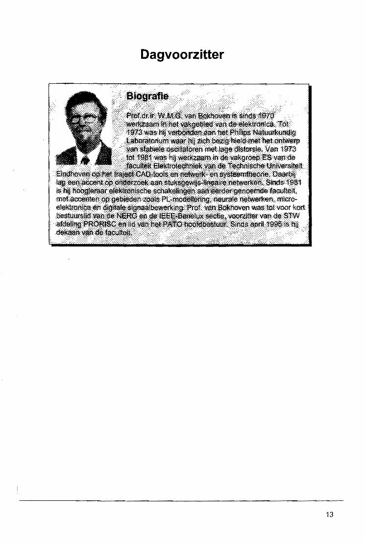
Dagvoorzitter: prof.dr.ir W.M.G. van Bokhoven

9.00 Ontvangst en koffie

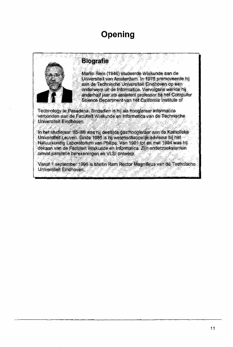
9.30 Welkomstwoord door prof.dr. M. Rem Rector Magnificus, TUE

9.45 Principes, mogeliJkheden en beperklngen van artlficiele neurale netwerken Prof.dr.ir. J. Vandewalle, Faculteit Toegepaste Wetenschappen, KU Leuven

10.30 Koffiepauze en informatiemarkt

11.00 Leren te redeneren Dr. H.J. Kappen, Stichting Neurale Netwerken, KUN

11.30 Neurale Netwerken gebruiken blj data-analyse Ir. J. van Dommelen, SAS Institute B. V.

12.00 Hardware neurale netwerken: analoog versus digitaal Dr.ir. A.J. Annema, Philips NatLab

12.30 Lunchpauze en informatiemarkt

13.30 Parallelle sessles over toepassingen

15.00 Theepauze en informatiemarkt

15.30 Forumdiscussie

16.00 Computer simulations of visual neurons: bar and grating cells Prof. dr. N. Petkov, Centre for High Performance Computing, Instituut voor Wiskunde en Informatica, RUG

16.45 Afsluiting door dClgvoorzitter, barrel

Parallelle sessies over toepassingen

Sessie 1 onder leiding van prof.dr. P.A.J. Hilbers:

13.30 Onderzoek naar neurale netwerken bij Shell Dr.ir. M.A. Kraayveld, Shell International Exploration and Production B. V.

14.00 Kunstmatlge neurale netten In de financliile dlenstverlening Drs. D.J.N. Egberts, Biologica

14.30 Conditlebewaklng van een dieselmotor met behulp van neurale netwerken Ir. PP. Meiler, TNO-FEL

Sessie 2 onder leiding van prof.dr. W.M.G. van Bokhoven:

13.30 Garens spinnen met neurale netwerken en genetische algorltmen Dr. A.P. de Weyer, AKZO Nobel Central Research

14.00 Neurale netwerken bij Smit Transformatoren Ing. H. Brockmeyer, Smit Transformatoren

14.30 Neurale netwerken in de energiesector; twee praktijkvoorbeelden Ir. R.M.L Frenken, KEMA

7

Inhoud

Voorwoord ........................................................................................................ 5

Programma ...................................................................................................... 6

Parallelle sessies over toepassingen ............................................................... 7

Opening ......................................................................................................... 11

Dagvoorzitter .................................................................................................. 13

Principes, mogelijkheden en beperkingen van artificiele neurale netwerken. 15

Leren te redeneren ........................................................................................ 27

Neurale netwerken gebruiken bij data-analyse .............................................. 33

Neurale Netwerken: Analoog versus Digitaal. ................................................ 41

Middagsessie 1 oJ.v. prof.dr. P.A.J. Hilbers .................................................. 57

Onderzoek en Toepassingen van Neurale Netwerken bij Shell ..................... 59

Kunstmatige neurale netwerken in de financiele dienstverlening .................. 63

Condition monitoring of a diesel engine by analysing its torsional vibration, using modern information processing technology .......................................... 69

Middagsessie 2 o.l.v. prof.dr.ir W.M.G. van Bokhoven .................................. 85

Garens spinnen met neurale netwerken en genetische algoritmen ............... 87

Neurale Netwerken bij Smit Transformatoren ................................................ 95

Neurale Netwerken in de energiesector; twee praktijkvoorbeelden ............... 99

Computational models of visual neurons specialised in the detection of periodic and aperiodic oriented visual stimuli: bar and grating cells ........... 107

IEEE SBE; Faculteit Wiskunde & Informatica; Rekencentrum ..................... 135

Dankwoord ................................................................................................... 137

Comite van aanbeveling .............................................................................. 139 Lijst van sponsors ........................................................................................ 141 Symposiumcommissie 1997 ........................................................................ 143

9

Opening

11

Dagvoorzitter

13

14

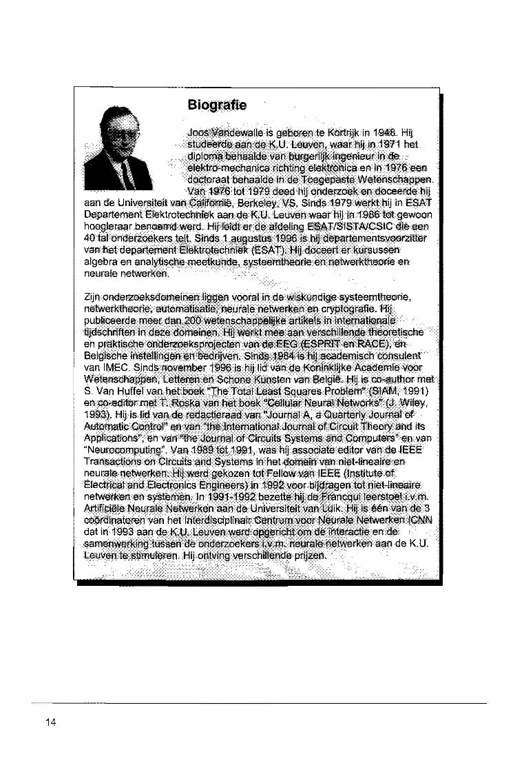
Biogr-.fie

Joo~~andewaftejl; g~J~rl te Kortfrjjkin 19148. Hij studeerde'aan waarhiHn1f971 het

" giploma=behaalde in de ::'elektro-mechanica. en in 19i'6 e. doctoraat behaalde in W~tenscllaP(3en. " Van 19c16 tot 1919 deed hij en deceerde hij

aan de Universit~tvan Califeqie, Berkeley, VS. Sinds 1919 werkt fuij in ESAT Departement ElektrotecBtIle'k ean de K.U.keuven :Wear hij i:t7l1936 tstgewoon hoeglEar:l:l~r b~l"1~qYJerd. HfJleidt er de afd~ling _TJ$tSTAlCSIC dieeef'l 40 taIOnaeffQek~~ Sinas·1.SiJ~J996 iship~artementsV0~itter v8llPlaet departeme rQt~c " (ESIlT). "Fiijdoceert er kursussen algebra enanalytiscllle~t~l?JRtle, systeemttJieorieen netwerktheone en neurale ne'twerken.

ZjjJ:l:QnGte~ek~einen Iiggen vooral in de Wisk,l;:lail'l!l systeemtf:reefie. netwefrktheorie. :fttematisatie. ne.urale netwe~k~n ct1Ptografie. Mij publiceerde mee~dawet~pschappil!l.lUke a .. rninternati~~I~ tijdschriften in de~e . en. 'fllJ wsrkt meaaan verschilltneoreti~:ciile en pf(aRtisoneQnder:toek~projecten varrde E~,Bn Bet~ische insfefUngenenFJedrijven. Sin~::~~ .' misch~.t1lent van IMeC. ·t;ld.l3::n8~~~~r,t9g6 is hij lid~ de~ . .. ... ijke Acade."te voor Wetefll.s1f3 '.. ., I.s~~O"~Schone Kunsten van B~lIie;ri~i~oo"91uth()r met S. Van Huffel vanh~tdfiO~·:Ih~!otal~L..Q~§t ~~~.res ... ... .' , ,1991 ) en~edi.pmet T.~ska van he.tboek '!~lmit~~,urarNetworWitey, 1993). . rliarA.a~t:Jarterly f

. of Circuit Theory and its of Circuits Systems anCi.Q~mp.uters" en van

"Neurocomputing?'. \teEt. . .' was hij associate editor v~n .. deIEt:E Traa$actions on Clrcuilsand Systems in hetd~~fnvan n·i@ft .. ltneair~xe{l new'ale netwerkel"l, Hijwerd gekozen totFellow~tf!J E.E5¢lnstitute. Elee:irica.1 and Ela sEngineers) in1t992 tot niet-I~ire netwer~nen In 1991-1992bezefte hij ui leers~§i.v.m. Artifig~le N~up§le de Universiteit Hij is eemvan de 3 coOrdin'St~~~rtvan hetfGMN. dat in 1993 aande.' , Leuve~ samenwerking t .. ·'td'eonderzoekers i. . Leuven te stimt:ll~;'ef1.HU<oQtving· veIschilfend~. prijzeB.

Principes, mogelijkheden en beperkingen van arti'ficiele neurale netwerken

Prof. dr. ir. Joos Vandewalle Departement Elektrotechniek (ESAT) Faculteit Toegepaste Wetenschappen

Kardinaal Mercierlaan 94, 3001 Heverlee Tel 321052 ; fax 321986

email: joos.vandewalle@esat.kuleuven.ac.be

Arlificiijle neurale netwerken bieden zich aan als aantrekkelqke altematieven voor de traditioneJe digitale Von Neumann computer omwille van verschillende redenen: de inherente parallel/e werking, de snelle ontwikkellngstijd, de eenvoud om een taak aan fe leren uifgaande van voorbeelden, de robuustheid tegen fouten, onnauwkeurigheden en defecten. Daarom hebben artificie/e neurale netwerken heel wat interesse gekregen voor technische toepassingen waar sensoriele gegevens verwerkt worden zoals s;gnaalverwerking, beeldverwerking, patroonherkenning, robotsturing, niet-lineaire model/ering en voorspelling. Bovendien lenen arlifide/e neura/e netwerken zich ook voor elektronische chipimplementatie.

Inleiding

Deze lezing heeft de volgende 6 doelstellingen: Vooreerst een vergelijking maken met voor- en nadelen tussen artifici~le neurale netwerken en digitale compu~er. Ten tweede het inzicht bijbrengen dat artifici~le neurale netwerken niet werken op basis van magische principes, maar moeten geanalyzeerd en ontworpen worden met grondige en door wiskunde onderbouwde methodes. Ten derde een bespreking geven van de toepassingsdomeinen waar artifici~le neurale netwerken enerzijds en de digitale computer anderzijds de voorkeur genieten. Ten vierde een overzicht bieden van een aantal aantrekkelijke toepassingen van artifici~le neurale netwerken. Ten vijfde een bespreking geven van hoe men te werk moet gaan om artifici~le neurale netwerken te gebruiken in allerhande technische, organizatorische en economische toepassingen. Ten zesde wijzen op de beperkingen van artifici~le neurale netwerken t.o.v. de menselijke hersenen. Ten laatste wijzen op de vooruitzichten voor het gebruik van artifici~le neurale netwerken in produkten.

Wat is een neuraal netwerk ?

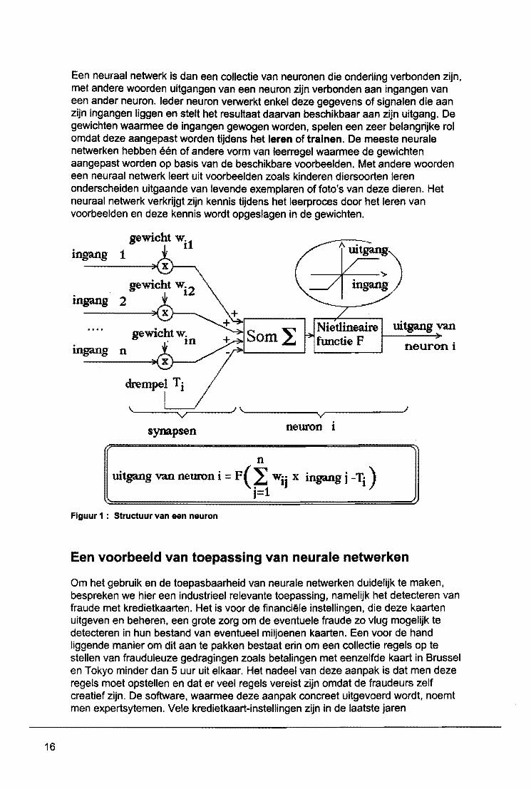
Vooreerst is het belangrijk om op te merken dat we in deze tekst altijd de term neurale netwerken gebruiken om er de "artificie/e" neurale .netwerken mee te beschrijven. Hiermee bedoelen we dus de mathematisch gedefinieerde modellen van netwerken bestaande uit artifici~'e neuronen. leder neuron maakt een gewogen som van zijn ingangen en verwerkt het resultaat daarvan in een niet-lineaire activatiefunctie (zie figuur 1). Dit soort neurale netwerken mag men niet verwarren met de biologische neurale netwerken, die veel ingewikkelder zijn dan de wiskundige en artifici~le tegenhangers hiervan.

15

16

Een neuraal netwerk is dan een collectie van neuronen die onderling verbonden zijn, met andere woorden uitgangen van een neuron zijn verbonden aan ingangen van een ander neuron. leder neuron verwerkt enkel deze gegevens of signalen die aan zijn ingangen liggen en stelt het resultaat daarvan beschikbaar aan zijn uitgang. De gewichten waarrnee de ingangen gewogen worden, spelen een zeer belangrijke rol omdat deze aangepast worden tijdens het leren of tralnen. De meeste neurale netwerken hebben een of andere vorm van leerregel waarmee de gewichten aangepast worden op basis van de beschikbare voorbeelden. Met andere woorden een neuraal netwerk leert uit voorbeelden zoals kinderen diersoorten leren onderscheiden uitgaande van levende exemplaren of foto's van deze dieren. Het neuraal netwerk verkrijgt zijn kennis tijdens het leerproces door het leren van voorbeelden en deze kennis wordt opgeslagen in de gewichten.

gewicht wi1

Ingang 1

lOgang

uitgang van

neuron i

\.'----=~;::::!..-----) \.'---------.. -------') v-

synapsen neuron 1

n

uitgang van neuron i = F (~ Wij x ingang j -Tj ) 1=1

Figuur 1 : Structuur van &en neuron

Een voorbeeld van toepassing van neurale netwerken

Om het gebruik en de toepasbaarheid van neurale netwerken duidelijk te maken, bespreken we hier een industrieel relevante toe passing. namelijk het detecteren van fraude met kredietkaarten. Het is voor de financiele instellingen. die deze kaarten uitgeven en beheren, een grote zorg om de eventuele fraude zo vlug mogelijk te detecteren in hun bestand van eventueel miljoenen kaarten. Een voor de hand liggende manier om dit aan te pakken bestaat erin om een collectie regels op te stellen van frauduleuze gedragingen zoals betalingen met eenzelfde kaart in Brussel en Tokyo minder dan 5 uur uit elkaar. Het nadeel van deze aanpak is dat men deze regels moet opstellen en dat er veel regels vereist zijn omdat de fraudeurs zelf creatief zijn. De software. waarmee deze aanpak concreet uitgevoerd wordt. noemt men expertsytemen. Vele kredietkaart-instellingen zijn in de laatste jaren

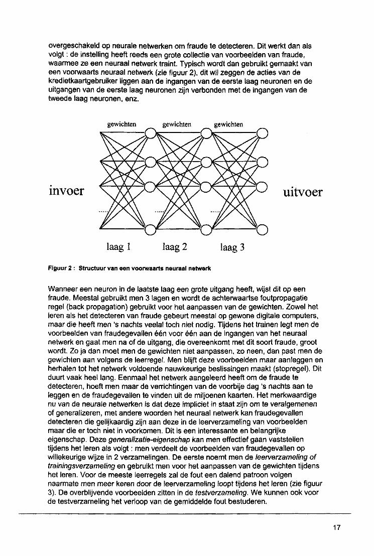
overgeschakeld op neurale netwerken om fraude te detecteren. Oit werkt dan als voigt: de instelling heeft reeds een grote collectie van voorbeelden van fraude, waarmee ze een neuraal netwerk traint. Typisch wordt dan gebruikt gemaakt van een voorwaarts neuraal netwerk (zie figuur 2), dit wi! zeggen de acties van de kredietkaartgebruiker liggen aan de ingangen van de eerste laag neuronen en de uitgangen van de eerste laag neuronen zijn verbonden met de ingangen van de tweede laag neuronen, enz .

. InVOer uitvoer

laag 1 laag2 laag 3

Flguur 2: Structuur van een voolWaarts neuraal netwerk

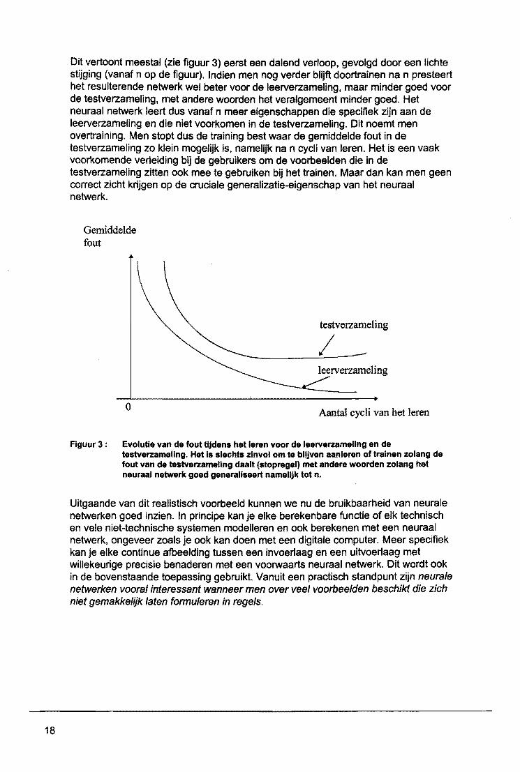
Wanneer een neuron in de laatste laag een grote uitgang heeft. wijst dit op een fraude. Meestal gebruikt men 31agen en wordt de achterwaartse foutpropagatie regel (back propagation) gebruikt voor het aanpassen van de gewichten. Zowel het leren als het detecteren van fraude gebeurt meestal op gewone digitale computers, maar die heeft men 's nachts veelal toch niet nodig. Tijdens het trainen legt men de voorbeelden van fraudegevallen een voor een aan de ingangen van het neuraal netwerk en gaat men na of de uitgang, die overeenkomt met dit soort fraude, groot wordt. Zo ja dan moet men de gewichten niet aanpassen, zo neen, dan past men de gewichten aan volgens de leerregel. Men blijft deze voorbeelden maar aanleggen en herhalen tot het netwerk voldoende nauwkeurige beslissingen maakt (stopregel). Oit duurt vaak heel lang. Eenmaal het netwerk aangeleerd heeft om de fraude te detecteren, hoeft men maar de verrichtingen van de voorbije dag '5 nachts aan te leggen en de fraudegevallen te vinden uit de miljoenen kaarten. Het merkwaardige nu van de neurale netwerken is dat deze impliciet in staat zijn om te veralgemenen of generalizeren. met andere woorden het neuraal netwerk kan fraudegevallen detecteren die gelijkaardig zijn aan deze in de leerverzameling van voorbeelden maar die er toch niet in voorkomen. Oit is een interessante en belangrijke eigenschap. Oeze generalizatie-eigenschap kan men effectief gaan vaststellen tijdens het leren als voigt: men verdeelt de voorbeelden van fraudegevallen op willekeurige wijze in 2 verzamelingen. De eerste noemt men de leerverzameling of trainingsverzameling en gebruikt men voor het aanpassen van de gewichten tijdens het leren. V~~r de meeste leerregels zal de fout een dalend patroon volgen naarmate men meer keren door de leerverzameling loopt tijdens het leren (zie figuur 3). De overblijvende voorbeelden zitten in de testverzameling. We kunnen ook voor de testverzameling het verloop van de gemiddelde fout bestuderen.

17

18

Oit vertoont meestal (zie figuur 3) eerst een dalend verloop. gevolgd door een lichte stijging (vanaf n op de figuur). Indien men neg verder blijft doortrainen na n presteert het resulterende netwerk wei beter voor de leerverzameling, maar minder goed voor de testverzameling, met andere woorden het veralgemeent minder goed. Het neuraal netwerk leert dus vanaf n meer eigenschappen die specifiek zijn aan de leerverzameling en die niet voorkomen in de testverzameling. Oit noemt men overtraining. Men stopt dus de training best waar de gemiddelde fout in de testverzameling zo klein megelijk is, namelijk na n cycli van leren. Het is een vaak voorkomende verleiding bij de gebruikers om de voorbeelden die in de testverzameling zitten ook mee te gebruiken bij het trainen. Maar dan kan men geen correct zicht krijgen op de cruciale generalizatie-eigenschap van het neuraal netwerk.

Gemiddelde fout

o

testverzameling

I

Aantal cycli van het leren

Figuur 3 : Evolutle van de fout tlJdens het leren voor de leerverzamellng en de testverzamellng. Het Is slechts zlnvol om te blljven aanleren of trainen zolang de fout van de testverzamellng daalt (stopregel) met andere woorden zolang het neuraal netwerk goad generallseert namellJk tot n.

Uitgaande van dit realistisch voorbeeJd kunnen we nu de bruikbaarheid van neurale netwerken goed inzien. In principe kan je elke berekenbare functie of elk technisch en vele niet-technische systemen modelleren en ook berekenen met een neuraal netwerk, ongeveer zoals je ook kan doen met een digitale computer. Meer specifiek kan je elke continue afbeelding tussen een invoerlaag en een uitvoerlaag met willekeurige precisie benaderen met een voorwaarts neuraal netwerk. Oit wordt ook in de bovenstaande toepassing gebruikt. Vanuit een practisch standpunt zijn neura!e netwerken voora! interessant wanneer men over veel voorbeelden beschikt die zich niet gemakkelijk laten formuleren in rege/s.

Vergelijking tussen dlgitale computer, biologisch neuraal netwerk en artificieel neuraal netwerk

lowel vanuit een conceptueel als vanuit een practisch standpunt is het nuttig om het onderscheid tussen de twee en de sterke en zwakke punten van elk te kennen.

Vooreerst bespreken we het werkingsprincipe. De digitale computer, dit wil zeggen de klassieke computer, die in de praktijk kan voorkomen als een kleine microcomputer, een huiscomputer, PC of een grote computer werkt altijd volgens het Von Neumann principe. le verwerken symbolen of getallen en in feite altijd "enen" of "nullen" en in een sequentie beschreven door een programma. De correctheid van de werking is gesteund op de wiskundige logica en de Boole algebra. Om deze computers goed te gebruiken hebben we software of programma's nodig. In computerwetenschappen en informatica heeft men daartoe een arsenaal van algoritmen, compilers, talen, ontwerpmethodieken ontwikkeld in de voorbije 30 jaar. Dit heeft geleid tot heel wat commerci~le producten en industri~le activiteit. In een neuraal netwerk daarentegen worden patronen verwerkt. In ons voorbeeld zijn dit de operaties met een specifleke kredietkaart. Oeze worden verwerkt door een niet­lineaire afbeelding via de neuronen uit de verschillende lagen zoals besproken in deel 2. De correcte werking moet dan bestudeerd worden aan de hand van de wiskundige studie van niet-lineaire functies. Wanneer er ook geheugenelementen en terugkoppelingen hiervan naar neuronen gemaakt worden, hebben we een verwerking als een niet-lineair dynamisch systeem. Oergelijke dynamische systemen worden wiskundig bestudeerd in de systeemtheorie en deze kunnen zeer wilde gedragingen vertonen tot en met chaotisch gedrag. Hier zijn nog heel wat open problemen. Bovendien is hier een nood aan een gelijkaardig arsenaal van ontwerpmethodieken en commerciele producten om efficj~nte en degelijke ontwerpen van neurale netwerken te maken (een aantal aspecten hiervan worden verder behandeld).

Ten tweede bespreken we de parallellisatie mogelijkheden. Terwijl een digitale computer de gegevens verwerkt in een sequentie van operaties is een neuraal netwerk per definitie parallel, dit wil zeggen aile neuronen van een bepaalde laag kunnen hun berekeningen in parallel uitvoeren. Oit levert meteen ook een groot voordeel op voor de neurale netwerken ten opzichte van traditionele algoritmen of rekenschema's. Immers om traditionele algoritmen effici~nt gebruik te laten maken van parallelle digitale computers moet men de programma's zodanig herschrijven of aanpassen dat de bewerkingen goed verdeeld zijn over de parallel of gelijktijdig werkende processoren zonder de correctheid van het programma aan te tasten. Voor een neuraal netwerk kan men aile berekeningen voor de neuronen uit een bepaalde laag vrij en gelijktijdig gaan uitvoeren in de verschillende processoren. De parallellisatie is dus gemakkelijk. Oit is een vorm van parallellisme die we ook in onze hersenen gebruiken.

19

20

Een derde onderscheid is het leren of trainen. Te rwij I een digitale computer waardeloos is als er geen software voor geschreven is, is een neuraal netwerk waardeloos als het niet getraind is. Het is trouwens vaak zo dat men in vele industriele toepassingen een groter budget voorziet voor software dan voor hardware (toestellen). Dus, wat de software is voor een digitale computer dat zijn de leerverzamelingen en de leerregel voor neurale netwerken. Een goede keuze van de leerregel en een gevarieerde collectie van voorbeelden in de leerverzameling en testverzameling zijn dan ook cruciaal voor een goede werking van een neuraal netwerk in toepassingen. Dit is intu'itief ook duidelijk wanneer we dit verge!ijken met het biologisch leergedrag.

Een vierde belangrijk onderscheid is de robuustheid en de rigiditeit. Digitale computers zjjn rigide, dit wil zeggen ze werken volgenszeer precieze regels en iedere wijziging, zelfs maar van een bit kan serieuze gevolgen hebben op de resultaten. Denken we maar weer aan de kleine fout in de Pentium-processor. Neurale netwerken daarentegen zijn robuust zoals onze hersenen. Ze zijn veel minder gevoelig aan onnauwkeurigheden in de gegevens, en hebben een interessante foutverbeterende capaciteit. Ze halen hun werking uit het collectieve . gedrag van het geheel van de neuronen en zijn aldus bestand tegen het defect raken van bepaalde neuronen, met andere woorden, wanneer een beperkt aantal neuronen defect raakt, zal dit slechts geleidelijk een verslechtering van de werking te weeg brengen. Het besluit uit deze vergelijking is dan ook dat de neurale netwerken sterk verschillend zijn van de digitale computers. Vandaar dat men spreekt van een nieuw paradigma voor informatieverwerking. Het is ook duidelijk uit deze vergeljjking dat artificiele neurale netwerken heel wat nuttjge ejgenschappen overerven van biologische neurale netwerken. Tegelijk is het belangrijk om hier duidelijk te stellen dat de correcte werking van artificiele neurale netwerken niet gegarandeerd kan worden vanuit de analogie met biologische neurale netwerken. Inderdaad, deze analogie is veel te zwak om een ingenieur of informaticus vertrouwen te geven in de correctheid. De degelijke werking moet volgen uit de wiskundige analyse van de niet­lineaire afbeeldingen of van de dynamische systemen en uit computersimulaties. We moeten bovendien bescheiden blijven wanneer we de technische of artificiele neurale netwerken die heden gemaakt kunnen worden, vergelijken met de menselijke hersenen. De meest voorkomende uitvoering in hardware van neurale netwerken is in elektronische VLSI chip technologie. Terwijl de menselijke hersenen 1011 neuronen hebben, kan men nu slechts hoogstens een paar duizend artificiele neuronen in 1 VLSI chip zetten. Via simulaties op computers kan men netwerken met een paar honderdduizend neuronen bestuderen. Het verschil is nog zo groot dat men niet mag verwachten dat dit binnen de tijdspanne van een paar decennia kan overbrugd worden. De snelheid van werking van elektronische neurale netwerken als specifieke VLSI chip of gesimuleerd op een digitale computer is evenwel veel beter. Men kan ermee per seconde 30 tot 100 miljoen elementaire bewerkingen van vermenigvuldiging met een gewicht uitvoeren, terwijl biologische neurale netwerken reactietijden hebben van 1 tot 2 milliseconden. De energetische efficientie van biologische neurale netwerken is dan weer spectaculair beter. De hersenen hebben ongeveer 10-16 Joule per bewerking en per seconde nodig terwijl de beste computers nu ongeveer 10-6 Joule per bewerking en per seconde nodig hebben. De conclusie hieruit is dat de methodologie voor het ontwerp en het gebruik van artificiele neurale netwerken sterk verschillend is van deze van biologische neurale netwerken.

Fascinerende toepassingen en beperkingen van neurale netwerken

Uitgaande van deze vergelijking is het duidelijk dat neurale netwerken vaak beter zijn voor het uitwerken van cognitieve taken en voor het verwerken van meerdere sensorie/e gegevens, dit wit zeggen in toepassingen van visie, beeld en spraakherkenning, robotica, sturingen van objecten en automatizatie. Digitale computers zijn duidelijk superieur in rig ide toepassingen zoals elektronische werkbladen, boekhouding, simulatie, elektronische post, tekstverwerking. Er tekent zich duidelijk een profilering af van complementaire toepassingsdomeinen voor beide soorten rekensystemen, waarbij beide niet mekaars concurrent zijn, maar mekaar aanvullen en vaak samen gebruikt worden. Het is trouwens zo dat de meeste neurale netwerktoepassingen nu nog uitgevoerd worden op digitale computers. Men kan ook niet verwachten dat een getraind neuraal netwerk verantwoording atlegt waarom het tot een bepaald besluit komt. Denken we hier aan ons voorbeeJd. Daar kan men stell en dat het getraind neuraal netwerk niet een juridisch sluitend bewijs levert dat de gedetecteerde kredietkaarten frauduleus zijn, maar het kan weI uit miljoenen kaarten een paar potentieel frauduleuze kaarten uitvissen. Deze kaarten kan men dan manueeJ verder onderzoeken. Het overtuigend nut van neurale netwerken bestaat dus hierin dat het uit de miljoenen kaarten gemakkelijk de potentieel frauduleuze kaarten eruit haalt.

In deze tekst is het niet mogelijk om een degelijke beschrijving te geven van de vele overtuigende toepassingen van neurale netwerken. Er bestaat hiervoor een zeer uitgebreide Iiteratuur (honderden boeken, 10-tal tijdschriften, en meer dan 10 conferenties per jaar). Voor de beginneling zijn er boeken die de materie uitleggen zonder veel wiskunde, met veel practische raadgevingen en dicht bij het toepassingsdomein (zie referenties). Voor de gevorderden zijn er in de tijdschriften en conferentieverslagen enorm veel artikels te vinden met zeer brede waaier van toepassingen. We geven eerst een overzicht van de verschillende belangrijke categorieen van toepassingen en gaan dan in op een specifiek voorbeeld van de sturing van een voertuig.

Een eerste belangrijke klasse van toepassingen zijn de expertsystemen met neuraJe netwerken. We hebben hierin naast de succesvolle fraudedetectie bij kredietkaarten de fraudedetectie bij mobilofonie, de selectie van materialen in bepaalde corrosieve milieus en van bepaalde toepassingen in medische diagnose. Nauw aansluitend daarbij zijn aile patroonherkenningsproblemen van spraak, spraak~gestuurde computers, en telefonie waarin onder andere het Belgische high tech bedrijf Lernout en Hauspie een wereldfaam heeft. De herkenning van letters, cijfers, gezichten en beelden vormen andere onderwerpen met vele industriele beeldverwerkingsapplicaties. Denken we hier maar aan het herkennen van handschrift, adressen op briefomslagen, het zoeken van gezichten van criminelen in een gegevensbank aan de hand van bepaalde delen van het gezicht, het herkennen van autonummerplaten, enz. Vooral voor toepassingen in beeldverwerking zijn er ook speciale neurale netwerken ontwikkeld, cellulaire neurale netwerken genoemd, die aileen maar verbindingen hebben met hun naaste buren in een rooster en daarom gemakkelijk op een chip kunnen ge'implementeerd worden. In deze chips werkt ieder neuron dan op een beeldpunt en beschikt soms zelfs over een lichtgevoelige diode, waardoor het rechtstreeks een beeld kan opnemen in de chip.

21

22

Met deze chips probeert men een artificieel oog (ref. Spectrum) of apparatuur voor slechtzienden te ontwikkelen.

Een volgende belangrijke klasse van toepassingen zijn de neurale netwerken voor predictie en voorspelling. Hier zijn succesvolle realizaties in de financiele sector met de voorspelling van wisselkoersen, portefeuille-beheer met verbeteringen van 12.3% naar 18% per jaar, het voorspellen van het elektriciteitsverbruik dat cruciaal is in de elektriciteitssector omdat men geen elektriciteit kan opslaan en dus juist zo veel moet produceren als er gevraagd wordt. V~~r deze toepassingen heeft een buitenstaander dikwijls het vooroordeel dat de voorspellingen van neurale netwerken "magisch" zijn. Maar zoals we aan de hand van figuur 3 reeds aangetoond hebben kan en moet men de kwaliteit van de voorspellingen van het neuraal netwerk toetsen met de testvoorbeelden. Om de vele methodes voor voorspelling te vergelijkingen is er in 1992 (zie referentie) een competitie georganizeerd. Het was de bedoeling om een voorspelling te maken van de volgende 100 onbekende waarden van een gegeven tijdreeks van 1000 waarden. Deze tijdreeksen zijn zeer gevarieerd van aard, namelijk metingen van een NH3laser, computergegenereerde tijdreeksen van een chaotisch systeem, financiele gegevens (wisselkoersen tussen dollar en de Zwitserse frank), een onvoltooide fuga van Bach, astrofysische metingen van een variabele witte dwerg ster, fysiologische metingen van een patient met slaapstoornissen. Neurale netwerken kwamen hier duidelijk als de beste methodes naar v~~r. Het is belangrijk om hierbjj te vermelden dat er in deze competitie ook neurale netwerken bij de slechtste methodes hoorden. Dit bewijst eens te meer dat men met neurale netwerken goede resultaten kan halen, maar dat dit niet automatisch is of gegarandeerd is. Het moet ondersteund zijn door degelijke inzichten. wiskundige analyses en simulaties.

Neurale netwerken zijn ook succesvol voor optimalisatie, kwaliteitsverbetering en sturing van mechanische, chemische en biochemische productieprocessen. Hierbij zorgt de niet-lineariteit van het neuraal netwerk voor belangrijke verbeteringen ten opzichte van traditionele lineaire regelaars voor de sturing van inherent niet-lineaire systemen zoals de regeling van een dubbele inverse slinger.

We besluiten met een bespreking van een specifiek toepassingsvoorbeeld namelijk de autonome sturing van een voerluig met een neuraal netwerk (AL VINN project). Het is de bedoeling om een voertuig op de weg te houden zonder chauffeur. De wagen is uitgerust met een videorecorder met 30 x 32 beeldpunten en met een laserlocalizator die de afstand meet van de wagen tot de omgeving in een rooster van 8 x 32 punten. AI deze metingen 30 x 32 + 8 x 32 = 1216 vormen de ingangen van het neuraal netwerk. Dan hebben we een verborgen laag van 29 neuronen en een uitgangslaag van 45 neuronen. Deze uitgangen geven aan wat de stuLirrichting is die het voertuig moet aannemen. Ais het middelste neuron meest positief is, gaat het voertuig rechtdoor. Ais het meest rechtse meest positief is, rijdt het maximaal naar rechts en analoog voor links. Hiermee hebben we de architectuur van het neuraal netwerk vastgelegd. Het wordt nu geleerd om op de weg te rijden door opnamen te maken van 1200 combinaties van scenes, licht en distorties en met een mens als chauffeur. Hiermee wordt het neuraal netwerk getraind en getest in ongeveer een half uur rekentijd met achterwaartse foutpropagatie. De kwaliteit van het rijgedrag is voor snelheden tot 90 km/u vergelijkbaar met de beste navigatiesystemen die gesteund zijn op visie.

Het grote voordeel van neurale netwerken is hier de snelle ontwikkelingstijd. Navigatiesystemen vereisen een ontwikkelingstijd van verschillende maanden voor het ontwerp en de ontwikkeling van visie-software, parameter-aanpassingen, en programma-aanpassingen, terwijl methodiek met neurale netwerken op een half uur klaar is. De gereduceerde ontwikkelingskost is vaak een doorslaggevend voordeel voor neurale netwerken omdat het neuraal netwerk de essenti~le karakteristieken van het probleem kan in rekening brengen zonder dat deze expliciet moeten geformuleerd worden.

Enkele raadgevingen om neurale netwerken succesvol te gebruiken in toepassingen

De hoofdboodschap uit dit deel is dat het niet zo moeilijk is om neurale netwerken te gebruiken en dat er degelijke methodes zijn, die in vele gevallen goede resultaten opleveren. Dit neemt niet weg dat in dit onderzoeksdomein een grote vari~teit van methodieken bestudeerd wordt en dat er voor specifieke problemen meer ge~igende methodes betere resultaten kunnen opleveren.

In meer dan de helft van de toepassingen gebruikt men evenwel de aanpak die we hier beschrijven. Meer details over deze methodes vindt men in de referenties of in het artikel1

• We kunnen hier ook het gebruik van de world wide web nieuwsgroep2 in verband met neurale netwerken aanraden. Deze bevat onder andere verwijzingen naar gratis software en commerci~le software en hardware en antwoorden op frequent gestelde vragen in verband met neurale netwerken.

De frequent gebruikte aanpak verloopt dan als voigt. Het type van netwerk is een 3 laags voorwaarts neuraal netwerk dat dus bestaat uit 3 lagen neuronen tussen de ingang en de uitgang. De neuronen hebben allen een sensori~le niet- die op een vloeiende manier gaat van een negatieve verzadiging (~1) voor voldoende negatieve ingang van de nietlineariteit naar positieve verzadiging (+1) bij voldoende positieve ingang. Tussen de twee in hebben we het actieve gebied waarin het neuron nog niet ge~ngageerd is en meer gevoelig is aan wijzigingen tijdens het leren. De meest gebruikte leerregel is de achterwaartse fout propagatie-regel die in feite de gewichten aanpast in de richting van de steilste afdaling van de foutfunctie, met andere woorden de gewichten worden zo aangepast dat de foutieve voorspellingen van het neuraal netwerk verkleinen. De grootte van de stap is een parameter die de gebruiker moet kiezen. Als deze te klein gekozen wordt, verloopt het leerproces te voorzichtig en te traag en moet men soms honderdduizenden cycli van aile voorbeelden in de leerverzameling doorlopen. Als deze te groot gekozen wordt, gaat men veel sneller leren, maar dan heeft men het gevaar dat men de goede keuze van gewichten voorbijschiet door te grote roekeloze stappen. De grootte van het netwerk kan met de volgende vuistregels bepaald worden. Het aantal neuronen mag njet te

1 D. Hammerstom, "Working with neural networks·, IEEE Spectrum, pg. 46-53, July 1993

2 world wide web : URL:http://wwwipd.via.uka.de/-precheltlFAQlneural-net-faq.htmlnetwerkadres van een nieuwsgroep in verband met neurale netwerken, een 32-tal bladzijden frequent gestelde vragen en antwoorden in verband met neurale netwerken met onder andere verwijzingen naar commerciele en gratis software voor het simuleren van neurale netwerken en een gegevensbank van gegevens voor het trainen van neurale netwerken in toepassingen. Op een ander adres nl. http://www.neuronet.ph.kcl.ac.ukl vindt men ook heel wat informatie o. a. over software i.v.m. neurale netwerken.

23

24

groot zijn om de rekentijd van de training niet te lang te maken. Bovendien leidt een te groot netwerk ook tot overtraining. Oit houdt in dat het neuraal netwerk te veel vrijheidsgraden heeft, waardoor het te veel zaken leert die niet speciflek zijn voor het probleem maar wei voor de leerverzameling. Het mag ook niet te klein zijn anders kan men niet de essentiele karakteristieken van het probleem modelleren met het neuraal netwerk (slechte generalizatie).

De eerste en de voornaamste stap in het ontwikkelen van een neuraal netwerk is de creatie van de leer- en testverzameling van voorbeelden. Vaak kost dit 90 % van de tijd en inspanning. Oeze gegevens van de leer- en testverzameling zijn cruciaal voor een empirische aanpak zoals neurale netwerken. Slechte gegevens betekenen slechte neurale netwerken. De selectie van de relevante variabelen die men opmeet hangt sterk af van de toepassing. Op basis van de ervaring van de specialisten in het toepassingsdomein kan men de meest belangrijke parameters selecteren die een invloed hebben op de klassificatie. Ook is het belangrijk om deze gegevens te analyseren (correlaties, trends, cycli) en de passende bewerking vooraf uit te voeren, namelijk eliminatie van uitbijters of uitschieters (outliers), trendverwijdering, ruis uitmiddelen of uitfllteren, passende scalering, Fourier transformatie, en eliminatie van verouderde gegevens. Een volgende vraag is hoeveel voorbeelden er nodig zijn. Dit aantal en de varieteit moet in elk geval groot genoeg zjjn om een representatieve verzameling te zijn. Meer is beter, maar betekent ook een langere rekentijd vereist voor het leren. Een vuistregel zegt dat er in de leerverzameling 5 maal zoveel voorbeelden moeten zitten als er gewichten in het neuraal netwerk zitten. Het aantal voorbeelden in de testverzameling kan de he 1ft genomen worden van het aantal voorbeelden in de leerverzameling en de verdeling van de voorbeelden in leer- en testverzameling moet totaal willekeurig zijn, met andere woorden de moeilijke voorbeelden mogen niet exclusief in een van de twee zitten.

De finale ontwikkelingsstap is het leren en testen van het neuraal netwerk. Zoals vroeger opgemerkt moet men leren met de leerverzameling zo lang de fout voor de testvoorbeelden vermindert (zie flguur 3). Indien het probleem zich voordoet dat het neuraal netwerk slecht leert, dan moet men de netwerkarchitectuur aanpassen of de stapgrootte aanpassen. De doelstelling van het leren moet zijn om een netwerk te gebruiken dat groot genoeg is om de taak te leren en dat klein genoeg is om goed te generalizeren. Hierbij kan men opmerken dat men het aangeleerde netwerk achtgeraf goed moet evalueren, want, zoals bij de mensen, kan een neuraal netwerk iets anders leren dan hetgeen de gebruiker had verwacht.

Besluiten en vooruitzichten op commerciele exploitatie

Neurale netwerken vormen dus nieuwe, alternatieve en realistische manieren om een ruime klasse van technische problemen op te lossen. Ze leren hun taak uit voorbeelden en vormen aid us een alternatief voor moeilijke en complexe software ontwikkelingen. Ze zijn vooral superieur voor cognitieve taken en taken waar sensoriele gegevens verwerkt worden zoals visie, beeld- en spraakherkenning, stu ring, robotica, expertsystemen. Er is heel wat software voor PC's beschikbaar zodat men er snel mee van start kan gaan.

De correcte werking mag en kan men niet aantonen met de biologische analogie maar uit wiskundige analyse en uit computersimulaties. De technische neurale netwerken zijn trouwens nog belachelijk klein in vergelijking met onze hersenen. Wei kan men vaak goede suggesties voor technische neurale netwerken uit biologische systemen halen. Eveneens kan men een aantal fenomenen (zoals visuele illusies, Cyclope"ische perceptie en stereoscopie) die zich voordoen in de hersenen goed modelleren met technische neurale netwerken.

Op dit ogenblik is de kennis en zijn de inzichten nog niet in het rijpere stadium waarin de informatica voor digitale computers heden is, maar er tekent zich duidelijk een complementariteit af tussen de digitale en de neurale computers. Terwijl er heden zeer veel digitale microprocessorchips gebruikt worden in allerhande producten van telecommunicatie (GSM), consumenten elektronica, audio, video, automatizatie, auto, medische apparatuur en spelletjes, kan men verwachten dat binnen een periode van 5 tot 10 jaar vele producten op de markt zullen komen waar sensoriele gegevens verwerkt worden met neurale processoren. Zo'n neuroprocessor chip kan dan zijn taak leren uit voorbeelden en aldus optimaal inspelen op specificiteiten van de gebruiker. We denken hierbij bijvoorbeeld aan het stemgestuurd werken met allerhande apparatuur, en het gebruik van de pen als ingang voor computers. Er zijn hier heel wat fascinerende ontwikkelingen mogelijk, waarvan we de volledige draagwijdte nog niet kunnen overzien.

Referenties

Zurada J., Introduction to artificial neural systems, West Publ. Co, St. Paul, 1992

Desmeth H. en Beale M., Neural network toolbox for use with Matlab, User's Guide,The MathWorks Inc., Netwich Mass., 1992, 1994.

Hammerstrom D., Neural networks at work, IEEE Spectrum, pp. 26-32, June 1993

Haykin S., Neural networks, A comprehensive foundation, MacMillan College Publ. Co., IEEE Press, Englewood Cliffs, 1994

Roska T. en Vandewalle J. (Eds.) Cellular neural networks, John Wiley & Sons, U.K., 1993

Weigend A.S. en Gershenfeld N.A. Time-Series Prediction: Forecasting the Future and Understanding the Past, SFI Studies in the Sciences of Complexity, Proc. Vol. XV, Addison-Wesley, Reading, MA, 1994.

Braham R. (Special report editor), Toward an artificial eye, IEEE Spectrum, pp. 20-69, May 1996

25

26

Biografie

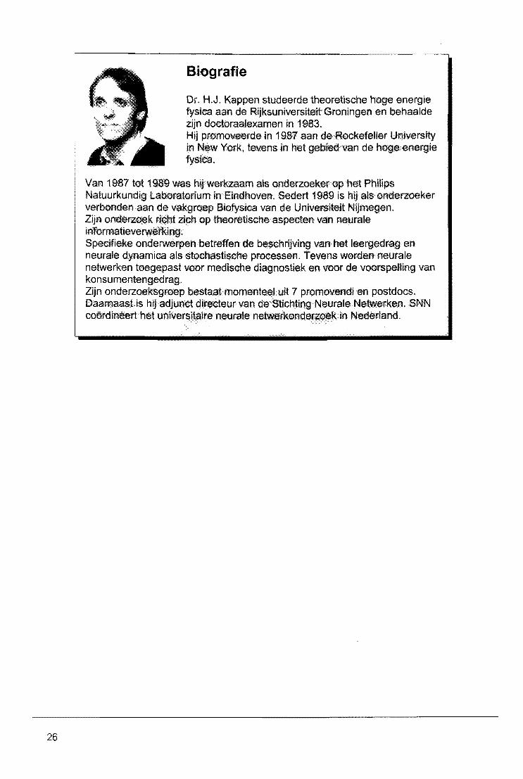
Dr. H.J. Kappen studeerde theoretische hoge energie fysica aan de Rijksuniversiteit Groningen en behaalde zijn doctoraalexamen in 1983. Hij promoveerde in 1987 aan de Rockefeller University in New York, tevens in het gebled van de hoge energie fys/ea.

Van 1987 tot 1989 was hijwerkzaam als onderzoeker op hat Philips Natuurkundig Laboratorium in Eindhoven. Sedert 1989 is hij als onderzoeker verbonden aan de vakgroep Biofysica van de Universite'it Nijmegen. Zijn onderzGEik ri~t zich op theoretische aspecten van neurale informatieverwerking. Specifieke onderwerpenbetreffen de beschrijving van het leergedrag en neurale dynamica als stochastische processen. Tevens worden neurale netwerken toegepast voor medische diagnostiek en voar de voorspelling van konsumentengedrag. Zijn onderzoeksgroep bestaatmomenteef. uit 7 promovendi en postdoes. Daamaast is hij adjunct d.iteeteur van de Stict:lting Neurale Netwerken. SNN coordineert het univers/tatre neurale netwerkornderzoek in tslededand.

Leren te redeneren

H.J. Kappen Stichting Neurale Netwerken, KUN

Neurale netwerken kunnen leren. Daarin zijn ze echter niet uniek. Bepaalde expert systemen, statistische algoritmes en methodes uit de machine learning kunnen dat ook. Het leren bestaat in aile geval/en uit het optimaliseren van model parameters via een kostencriterium dat afhangt van de 'data', of in neurale termen, de trainingsvoorbeelden. Het succes van het leren wordt volledig bepaald door een goede keuze van het model. In die zin bestaat leren dus ook uit mode/se/ectie. Neurale netwerken zijn met name zo succesvol vanwege de verzameling modellen die ze omvat. De milde niet-lineariteft die wordt verkregen door toevoeging van hidden units blijkt in de praktijk vaak succesvol. In dft verhaal zal het prob/eem van mode/se/ectie worden geillustreerd in de context van redeneren met onzekerheid. Dit vereist het leren van een kansverde/ing over aile prob/eemvariabe/en. Oft probleem is in het algemeen 'ill-posed' vanwege het grote aantal mode/parameters verge/eken met het aantal trainingsvoorbeelden. De oplossing is het representeren van de kansverdeling door een sparse neuraal netwerk. Het modelselectleprobleem is nu welke verbindingen weI en niet 'nodig' zijn.

Introduction

Traditional rule-based systems based on pure logic are incapable of handling uncertain (imprecise, incomplete or inconsistent) data. The issue is especially problematic for real world applications, where complete knowledge is not possible, except in very trivial situations. The various attempts to include uncertainty into knowledge representations can be grouped into two types of approaches, called extensional or rule-based and intentional or model-based [5]. Extensional approaches are the expert systems of the 1970s that assign certainty weights to rules and facts and use heuristics for the calculation of weights for combinations of rules and facts. These systems payed relatively little attention to the theory of probability. The primary organizing idea was still symbolic logic. An example of an extensional system is the MYCIN system for diagnosing bacterial infections. Extensional systems are computationally convenient but semantically limited. It has been shown, that the heuristics can be interpreted as probabilistic reasoning when certain independence assumptions are made. Unfortunately, in many problem domains these assumptions are not valid. Recently, uncertain reasoning systems based on fuzzy logic have gained popularity, especially in Japan. However, it has been shown that any consistent computational framework representing some degree of uncertainty has to be based on axioms of probability theory.

Intentional systems are based on probability theory, and combine facts and rules using the rules of probability. Intentional systems are semantically clear but are often computationally intractable: The computation time required for an inference problem is in general exponential in the problem size. In general, the computational complexity of learning in these networks is the same as for inference.

27

28

Therefore, an important research topic is to design robust and consistent reasoning systems that are computationally efficient. In addition, these systems should be able to learn from data, and should be able to incorporate structural domain knowledge. After training the system should be able to give rules that are buried in the data, and provide explanation regarding its decisions. A robust solution of this type will automatically provide a mechanism for dealing with inconsistencies and missing values.

Another important reason to cast the learning problem in terms of a probability estimation problem is to better understand the 'reasoning' used by a network to reach a decision, i.e. for rule extraction from a trained network. An advantage of the probabilistic approach over the extensional approach is that one can train a probabilistic model from data, without specifying in advance the type of rules that one is interested in. After training, one can extract either predictive rules (from cause to effect) or diagnostic rules (from effect to cause) or both, without running into inconsistencies. Our active decision method is an example of such an approach. This is not possible in any of the extensional systems.

Bayesian networks and Boltzmann Machines

There are various approaches to model probability distributions. The most well­known is a method called Bayesian networks. Here, the probability distribution p(x1, ... ,x,J is written as a product P(X1)P(X2Ix1)P(X3Ix1,X:z) ... p(xnlx1"",Xn-1)' Each of the terms .in the product describes the probability of x, conditioned on all possible values of X1,. .. Xi_1• Therefore, exponentially many parameters must be fixed to define the total probability distribution. For instance, if Xi are binary variables, p(xilx1,. .. ,Xi_1) requires 2-1 parameters. The Bayes network is a directed graph with nodes as variables and links as the conditional probability tables. Note that the graph depends on the ordering of the nodes.

Thus, there are too many parameters to be fixed by the data, compared to available data. The typical way to solve this problem in the Bayesian network approach is to augment the data with domain knowledge from experts in the form of conditional independence statements. These are statements of the form that subset of variables A and subset of variables B are independent given the values of the variables in subset C, ie. p(A,BIC)=p(AIC)p(BIC). The effect of conditional independence statements is that the number of free parameters is reduced and that certain links in the graph can be deleted.

An alternative method is to use Boltzmann Machines for probability estimation. Although the representational power of the BM on the visible units is quite limited, it can be extended by the inclusion of hidden units. Such probability models are in principle capable of modeling arbitrary probability distributions. Properties of these models can be partially analyzed using techniques from statistical mechanics.

In the remaining of this paper, I will give an example of the application of probability models for medical diagnostiCS.

Active decision strategies

In many instances, intelligent behaviour requires to make decisions based on very limited and possibly contradicting information. The active decision paradigm is an idealization of this problem and provides a method to combine previously learned domain knowledge with partial, incomplete, observations to generate optimal actions. The actions consist of requests of additional pieces of information. The problem is how to reach a correct decision with a minimal number of actions.

Active decision problems occur in many real world applications

Diagnostic problems and dialogue maintenance are two examples. In the case of medical diagnostics, the patient presents the physician with a number of symptoms which provide information about the patients disease. Based on the likelihood of various possible diagnoses, the physician will request additional laboratory tests or other information to eliminate the existing uncertainty and to be able to make a final diagnosis. The expertise of the physician allows him or her to request the most informative additional information, thus requiring a minimum of additional tests.

More formally, the problem is defined as follows. Let an object be defined by a set of measurable attributes, which are collectively given by a vector X in a vector space U. We want to classify X in one of a number of classes a=1, ... ,C. The classification is performed in a number of steps. At time t=O, a limited number of components of X is given. The values of these components are not sufficient to define the class of x. At each time step an action is performed which consists of the measurement of one of the unknown components of x. After a number of time steps, sufficient components are known to decide the class of X. The problem is to find the minimal sequence of actions to make the correct decision.

The problem can be solved when two constraints are satisfied: 1) the joint probability on the product space of features and classes can be learned and 2) this jOint probability allows for efficient calculation of marginal probabilities.

In our approach we have found an elegant solution of 2). The reason is that the requirement for networks to have efficient learning rules is the same as the requirement to efficiently compute marginal probabilities. Problem 1) is an emperical question, whether sufficient data is available for training.

I

Active decision requires at the same time "a model for diagnosis and for prediction. Both models are needed to compute the optimal next action. It is therefore a non­trivial application of the powerful ideas of probability based reasoning.

Lab-Test Selection in Diagnosis of Anaemia.

One of the current problems in modern hospital management is the requests of unnecessary lab-tests for diagnostiC purposes. Unnecessary lab-tests do not only have financial consequences, but also increase the work-load of the hospital laboratories, causing longer waiting-times. Both have their clear impact on the quality of patient treatment.

29

30

One area in which this problem can be analyzed is in diagnosing anaemia type. Patients can suffer from several dozens of different types of anaemia. Thus, once the diagnosis of anaemia is established, the task of the physician is to determine which type of anaemia the patient is suffering from. For this task, about 200 lab-tests are at the physician's disposal. The problem is that in the clinical situation - in particular inexperienced - physicians tend to request far too many tests to make the diagnosis. The reason is that explicit text-book rules to decide when to do which tests are not sufficiently accurate. Physicians have to rely for a large part on their experience.

The benefits of an automated tool to optimize the selection of lab-tests are clear. However, due to the absence of a complete set of explicit rules, a rule-based decision tree is doomed to fail. On the other hand, the fact that physicians are able to learn to select the tests on the basis of increasing experience already indicates that positive results may be obtained using self-learning systems like neural networks.

In our application we combine the benefits of decision trees and neural networks. On the basis of a dataset of previously diagnosed patients - which is available in the hospital records - combined with prior expert knowledge a so-called Boltzmann Machine [3, 4] neural network (BM) is trained. After training, the BM is ready for use. Given the characteristics of the patient who is to be diagnosed, the BM predicts -on the basis of its trained experience- the amount of information which is to be expected from each lab-test. With these predictions, the physician can increase the efficiency of the. requested lab-tests. This application is intended as a medical tool in Dutch hospitals.

Results

The medical data for patients with anaemia to train the BM is obtained from the University Hospital in Utrecht. The number of possible diagnoses within anaemia is 51. The number of relevant lab-test which are included in the database is 91. For test runs a dataset with 281 cases is used. In this set, 40 cases contain a second diagnosis, and one a third diagnosis. We applied the leave-one-out method on each of the 281 cases. This means that for each case, a BM is trained on the complete dataset except the one case in question. After training the BM is tested on the remaining case. In the classification problem the BM selects the two most likely diagnoses on the basis of all the available features in the database of the case. If the most likely diagnosis given by the BM coincides with one out of possibly three diagnoses stated in the database the first performance index P1 is increased byone. If either the most likely or the second likely diagnosis of the BM coincides with one of the diagnoses in the database the second performance index P2 is increased by one. Note that P1 sP2 sN = 281. We also included domain knowledge from experts into the system. We asked medical experts to describe the typical lab-tests outcome for each diagnosis. We transformed this knowledge into a probabilistic model, which was supplemented to the data.

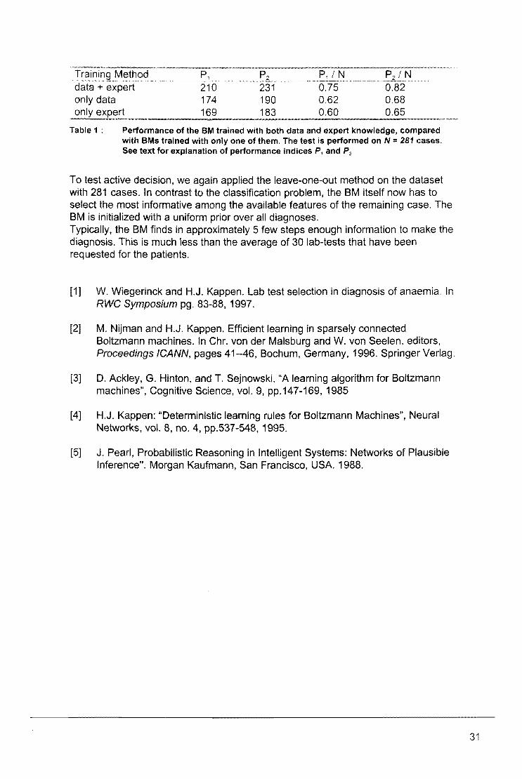
Method data + expert only data

231 190 183

0.75 0.62 0.60

0.82 0.68 0.65

Table 1 : Performance of the BM trained with both data and expert knowledge, compared with BMs trained with only one of them. The test is performed on N = 281 cases. See text for explanation of performance indices P, and P,

To test active decision, we again applied the leave-one-out method on the dataset with 281 cases. In contrast to the classification problem, the BM itself now has to select the most informative among the available features of the remaining case. The BM is initialized with a uniform prior over all diagnoses. Typically, the BM finds in approximately 5 few steps enough information to make the diagnosis. This is much less than the average of 30 lab-tests that have been requested for the patients.

[1] W. Wiegerinck and H.J. Kappen. Lab test selection in diagnosis of anaemia. In RWC Symposium pg. 83-88,1997.

[2] M. Nijman and H.J. Kappen. Efficient learning in sparsely connected Boltzmann machines. In Chr. von der Malsburg and W. von Seelen, editors, Proceedings ICANN, pages 41--46, Bochum, Germany, 1996. Springer Verlag.

[3] D. Ackley, G. Hinton, and T. Sejnowski. "A learning algorithm for Boltzmann machines", Cognitive Science, vol. 9, pp.147-169, 1985

[4] H.J. Kappen: "Deterministic learning rules for Boltzmann Machines", Neural Networks, vol. 8, no. 4, pp.537-548, 1995.

[5] J. Pearl, Probabilistic Reasoning in Intelligent Systems: Networks of Plausible Inference". Morgan Kaufmann, San Francisco, USA. 1988.

31

32

8iogliafie

JtJditf:l A. van Domm.&nis .in f99gafgestude~ als . ~iS1<\tJndig ingen~~aafla~lJtflJe~iteit Twent~7fij~ns

'1OgeCC5mlfneerde stag. w(ll~en)pmt~c~tt)i1CQMB.V. teSmrdRoven lIeeft .. ~j

Neurale netwerken gebruiken bij data­analyse

Inleiding

Ir. Judith A. van Dommelen SAS Institute B. V.

Een neuraal netwerk is onder andere een methode om gegevens te analyseren. Een methode waarmee kennis of informatie uit die gegevens gehaald kan worden. Door gegevens met neurale netwerken te analyseren, kunnen patronen of relaties opgespoord worden. Die opgespoorde "kennis" kan dan gebruikt worden bij voorspellen in situaties met vergelijkbare gegevens.

Mogelijkheden

Neurale netwerken kunnen heel geschikt zijn om een speciaal soort gegevens te analyseren: zeer complexe bestanden met daarin een sterke mate van niet­lineariteit. V~~r dergelijke bestanden zijn soms weinig andere geschikte analysemethodes voorhanden. De Neurale Netwerken Applicatie (NNA) is een uitbreiding van de software van SAS Institute voor data-analyse. De applicatie is in situaties met vele invloedsfactoren een krachtig middel. Een voorbeeld van een dergelijke situatie vindt men in een bestand met gegevens van klanten. Daarin kunnen sociaal-economische gegevens staan, zoals geslacht, leeftijd, burgerlijke staat, inkomen en opleidingsniveau, Bij een bank kan bijvoorbeeld ook het aantal leningen, of iemand een hypotheek afgesloten heeft, het aantal spaarrekeningen en het saldo op spaarrekeningen in een dergelijk bestand staan. Er zijn vele toepassingsgebieden denkbaar. In de tinanciele dienstverlening het opsporen van frauduleuze transacties met credit cards of het opsporen van frauduleuze claims bij (reis)verzekeringen. In de Informatie Technologie is het voorspellen van het CPU gebruik op een mainframe mogelijk. Oat CPU gebruik kan door veel factoren be"invloed worden, zoals het onderhoud aan een mainframe, de dag van de week en de aanschaf van PC's. Ais het patroon in het CPU gebruik opgespoord is, kan het gebruik in de toekomst beter voorspeld worden. Denk ook aan een toe passing waarbij gebruik gemaakt wordt van het protiel van klanten in een marketing database van een organisatie. Op welke klanten moet de organisatie zich richten bij een direct mail actie voor een bepaald produkt?

33

34

Voorwaarden voor succesvolle implementatie

In het algemeen geldt dat bij voorkeur met een urgent, duidelijk omschreven probleem gewerkt moet worden. Verder moeten experts die de gegevens kennen erbij betrokken worden en hangt het succes sterk af van de kwaliteit van de gegevens. Gebruik indien mogelijk schone, historische gegevens van hoge kwaliteit.

Het belangrijkste aandachtspunt bij de ontwikkeling van een neuraal netwerk is generalisatie: hoe goed zal het netwerk voorspellen v~~r gevallen die niet in het trainingsbestand zitten? Generalisatie is niet altijd mogelijk. Er zijn twee noodzakelijke (maar niet voldoende) voorwaarden voor goede generalisatie.

• De eerste is dat de te "Ieren" functie die de invoer aan de juiste uitvoer koppelt in zekere zin "smooth" moet zijn. Een kleine verandering in de input zou in de meeste gevallen een kleine verandering in de output moeten produceren.

• De tweede noodzake/ijke voorwaarde is dat de trainingsgegevens een voldoende grote en representatieve deelverzameling (steekproef) moeten zijn van de totale gegevensverzameling (populatie) waarnaar gegeneraliseerd moet worden.

Er zijn grofweg twee soorten generalisatie: interpolatie en extrapolatie. Interpolatie kan vaak vrij betrouwbaar uitgevoerd worden, maar extrapolatie is notoir onbetrouwbaar. Het is dus belangrijk om voldoende trainingsgegevens te hebben om de noodzaak van extrapolatie te vermijden. Het verzamelen van die gegevens kost de meeste inspanning. Bjj het verzamelen van gegevens is het van belang dat ze vooraf bewerkt of getransformeerd worden indien dat nodig is. Ze dienen ook uit dezelfde populatie te komen als de voorspeldata.

Neurale netwerken kunnen last hebben van overfitting of underfitting net als andere flexibele niet-lineaire schattingsmethoden (bijvoorbeeld kernel regressie). Een netwerk dat niet complex genoeg is zal niet het volledige signaal detecteren in een gecompliceerd gegevensbestand en zodoende tot underfitting leiden. Een netwerk daarentegen dat te complex is zal mogelijkerwijs de ruis titten en niet slechts het signaal en dus tot overfitting leiden. Overfitting kan bij veel gewone typen netwerken leiden tot voorspellingen die ver buiten het bereik van de trainingsdata liggen. Underfitting kan ook wilde voorspellingen produceren bij multilayer perceptrons, zelfs met data met weinig ruis. Underfitting produceert excessieve bias in de output, terwijl overfitting excessieve variantie produceert. Een manier om overfitting te vermjjden is grote hoeveelheden trainingsdata te gebruiken. Bij een vaste hoeveelheid trainingsdata zijn er effectieve benaderingen om underfitting en overfitting te vermijden en dus een goede generalisatie te krijgen.

Ruis in de actuele gegevens beperkt de nauwkeurigheid van generalisatie die bereikt kan worden, ongeacht hoe uitgebreid het trainingsbestand is. Maar kunstmatig ruis inbrengen in de input tijdens de training is een van de manieren om de generalisatie van "smooth" functies te verbeteren bij een klein trainingsbestand. Hoe meer bekend is over de verdeling van de ruis hoe effectiever het netwerk getraind kan worden (McCullagh & Neider, 1989).

Voor de controle en beoordeling van een neuraal netwerk geldt:

- een slecht trainingsnetwerk voorspelt ook slecht - een goed trainingsnetwerk kan slecht voorspellen - vergelijk indien mogelijk met de huidige technieken - vergelijk de voorspelling op termijn met de echte waarden - de generalisatiefout is van belang

Er zijn vele methoden om de generalisatiefout te schatten. • Een methode is maten gebruiken gebaseerd op een enkele steekproef zoals AIC,

SBC, RMSE en anderen bekend uit de statistiek. V~~r lineaire modellen verschaft de statistische theorie verscheidene schatters voor de generalisatiefout onder verschillende aannames (Darlington, 1968, Efron & Tibshirani. 1993). Deze maten kunnen ook gebruikt worden als grove schattingen van de generalisatiefout voor niet-lineaire modellen bij een groot trainingsbestand. Deze maten corrigeren voor niet-lineariteit vereist veel meer rekenkracht {Moody, 1992). en de theorie gaat niet altijd op voor neurale netwerken.

• De meest gebruikte methode om de generalisatiefout te schatten bij neurale netwerken is een deel van de gegevens te reserveren als testgegevens die op geen enkele andere manier tijdens de training gebruikt moeten worden. Die testgegevens moeten ook een representatieve steekproef vormen. Na de training wordt het netwerk met de testgegevens gedraaid en de fout van de testgegevens geeft een zuivere schatting van de generalisatiefout als de testgegevens random gekozen waren. Het nadeel van deze "split-sample" validatie is dat er minder gegevens beschikbaar zijn voor training en validatie (Weiss & Kulikowski, 1991).

• Cross-validation is een verbetering ten opzichte van "split-sample" validatie en biedt de mogelijkheid aile gegevens voor de training te gebruiken. Het nadeel hier weer van is dat het netwerk vele malen opnieuw getraind moet worden.

• Bootstrapping is weer een verbetering ten opzichte van cross-validation en geeft betere schattingen van de generalisatiefout ten koste van nog meer rekentijd.

Neurale netwerken en statistische methoden

Er is een aanzienlijke overlap tussen neurale netwerken en statistiek. In de terminologie van neurale netwerken, betekent statistisch toetsen leren te generaliseren uit data met ruis. Sommige neurale netwerken gaan niet over data­analyse (bv. de netwerken die bedoeld zijn om biologische systemen te modelleren) en hebben dus weinig te maken met statistiek. Sommige neurale netwerken leren niet (bv. Hopfield netwerken) en sommige netwerken leren aileen met succes met gegevens die vrij van ruis zijn. Maar vee I neurale netwerken die kunnen leren effectief te generaliseren uit gegevens met ruis lijken op of zijn identiek aan statislische methoden. Bijvoorbeeld:

• Feedforward netwerken zonder verborgen laag zijn eigenlijk gegeneraliseerde lineaire modellen . • Probabilistische neurale netwerken zijn equivalent aan kernel discriminant analyse . • Hebbian learning is verwant aan principale componenten analyse.

Er zijn ook enkele gebieden uit de neurale netwerkenwereld die geen nabije verwanten lijken te hebben in de bestaande statistische literatuur.

35

36

Feedforward netwerken zijn een deelverzameling van de klasse van niet-lineaire regressie en discriminant modellen. Veel resultaten uit de statistische theorie van niet-lineaire modellen kunnen direct toegepast worden op feedforward netwerken en de methoden die gewoonlijk gebruikt worden om niet-lineaire modellen te titten, zoals verschillende Levenberg-Marquardt en conjugate gradient algoritmen kunnen worden gebruikt om feedforward netwerken te trainen.

Er wordt soms beweerd dat neurale netwerken anders dan bij statistische modellen geen aannames over onderliggende verdelingen nodig hebben. Neurale netwerken brengen echter vaak dezelfde soort aannames over verdelingen met zich mee als statistische modellen. Statistici bestuderen de gevolgen en het belang van deze aannames, maar veel mensen die met neurale netwerken werken doen dat niet. Ais de aannames over verdelingen bestudeerd worden, kan het niet voldoen aan die aannames herkend worden en kan er rekening mee gehouden worden.

Werking neurale netwerken applicatie

Er worden twee fases onderscheiden bij het gebruik van de NNA, een trainingsfase en een voorspelfase. Het neuraal netwerk traint zichzelf, leert aan de hand van voorbeelden. Ais het netwerk getraind is, representeren de bestaande gewichten (getallen behorende bjj de verbindingen tussen neuronen) de "kennis" van het netwerk. Een getraind netwerk kan dan gebruikt worden om te voorspellen met andere gegevens.

Met de applicatie is het mogelijk verschillende typen netwerken te kiezen, zoals een multilayer perceptron of een radial basis function netwerk. De techniek die in de trainingsfase gebruikt wordt om de gewichten te berekenen kan ingesteld worden. Dit is vergelijkbaar met schattingsmethodes in de statistiek. De technieken zijn een aantal geoptimaliseerde numerieke routines. Via het instellen van een convergentiewaarde kan aangegeven worden hoe nauwkeurig de gewichten bepaald moeten worden. In de trainingsfase wordt code gegenereerd als een netwerk getraind wordt en die code kan gebruikt worden om verschillende netwerken in batch te trainen.

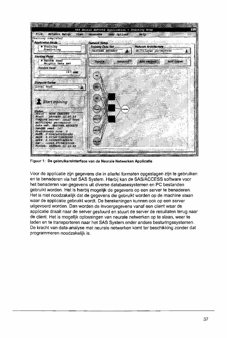
Figuur 1: De gebruikersinterface van de Neurale Netwerken Applicatie

Voor de applicatie zjjn gegevens die in allerlei formaten opgeslagen zijn te gebruiken en te benaderen via het SAS System. Hierbjj kan de SAS/ACCESS software voor het benaderen van gegevens uit diverse databasesystemen en PC bestanden gebruikt worden. Het is hierbij mogelijk de gegevens op een server te benaderen. Het is niet noodzakelijk dat de gegevens die gebruikt worden op de machine staan waar de applicatie gebruikt wordt. De berekeningen kunnen ook op een server uitgevoerd worden. Dan worden de invoergegevens vanaf een client waar de applicatie draait naar de server gestuurd en stuurt de server de resultaten terug naar de client. Het is mogelijk oplossingen van neurale netwerken op te slaan, weer te laden en te transporteren naar het SAS System onder andere besturingssystemen. De kracht van data-analyse met neurale netwerken komt ter beschikking zonder dat programmeren noodzakelijk is.

37

38

Conclusie

Bij gebruik van neurale netwerken voor data-analyse:

• kunnen statistische methoden nodig zijn om data vooraf te bewerken • zijn neurale netwerken specialisten nodig om het netwerk te bouwen en te trainen

en statistici om gegevens te bewerken • vertellen neurale netwerken niet waarom, dus kunnen in die zin statistische

modellen niet vervangen

Een goede netwerk topologie hangt sterk af van het aantal trainingsgegevens, de hoeveelheid ruis en de complexiteit van de te "Ieren" functie of classificatie. Er bestaat een behoorlijke overlap tussen neurale netwerken en statistiek. Die overlap wordt niet altijd herkend door verschillen in vakjargon. De Neurale Netwerken Applicatie is een snelle en flexibele methode om gegevens te analyseren waarbij geen modelbouw (zoals in de statistiek) of programmeerwerk nodig is. Het is een geschikte methode om zeer complexe, niet-lineaire gegevens te bewerken uit allerlei toepassingsgebieden en is te gebruiken om patronen op te sporen of toekomstige resultaten te voorspellen uit historische informatie.

Referenties

Darlington, R.B., "Multiple regression in psychological research and practice", Psychological Bulletin, vol 69 (1968), p.161-182.

Efron, B. & R.J. Tibshirani, An introduction to the bootstrap, Chapman & Hall, London, 1993.

McCullagh, P. & J.A. Neider, Generalized linear models, Second Edition, Chapman & Hall, London, 1989.

Moody, J.E., "The effective number of parameters: an analysis of generalization and regularization in nonlinear learning systems", NIPS vol 4, p. 847-854, 1992.

Weiss, S.M. & C.A. Kulikowski, Computer systems that learn, Morgan Kaufmann, 1991.

Maar hoe blijft u aan de top? Kennis is macht. Oat deze stelling veel waarheid bevat, beseft u als manager als geen

ander. De informatiestroom die u vandaag bereikt. vormt de leidraad voor uw beleid

van morgen. Met het topje van de ijsberg neemt u dan ook geen genoegen. U zoekt

het instrument dat u inzicht geeft in de ontwikkelingen die u belangrijk vindt, Niet

aileen boven, maar ook onder de waterlijn wenst u de essentiele informatie over

trends, klanten, marktontwikkelingen en uw eigen organisatie.

Organisaties staan bol van waardevolle data, opgeslagen in bestaande computer­

systemen. SAS Institute levert Data Warehouses: haarftjne instrumenten om data

binnen en buiten uw organisatie bijeen te brengen en om te zetten in eenduidige

informatie, Informatie die leidt tot kennis. Bekijkt u aileen de top, of overziet u de

hele berg?

Meer weten? Bel Judith Coster bij SAS Institute of stuur de bon in.

SAS Institute: Software for Successful Decision Making.

SAS Institute

Antwoordnummer 511

1270 VB Huizen

telefoon (035) 699 69 00

SAS Institute is specialist in Data Warehouse en

Business Intelligence toepassingen. Met vestigingen

in 120 landen en ruim 4.000 medewerkers onder~

steunt SAS Institute wereldwijd zo'n 30.000 klanten

bij hun kritische informatievoorziening.

la, Ik wI! graag meer Informatle over SAS Institute.

Naam:

Naam bedrijf:

40

Biografieen

Anne~Johan Annema studeerde in 1990 af bij de faculteit der elektrotechniek van de Universiteit Twente op het gebied van de analoge elektronica. In het daaropvolgende promotieonderzoek heeft hij gewerkt aan neurale netwerken. De nadruk hierbij lag op zowel het (mathematisch) analyseren van neurale netwerken en het afleiden van specificaties voor bouwblokken als op het implementeren van een neuraal netwerk in analoge hardware. Het proefschrift is als boek uitgegeven: "Feed-Forward Neural Networks: Vector Decomposition Analysis. Modelling and Analog Implementation" (Kluwer, 1995). Na zjjn promotie was hij 1 jaar werkzaam op de UT als wetenschappelijk mede werker. Sinds 1995 werkt hij bij hetPhilips Nat.Lab. te Eindhoven als wetenschappelijk medewerker.2ijn werkzaamheden betreffen onder meer onderzoek naar neurale netwerk hardware, naar nief-vluchtige geheugens, en onderzoek naar implementaties van analoge circuits in huidige en toekomstige CMOS processen.

F.P. Widdershoven studeerde in 1984 af aan de Faculteit der Elektrotechniek van de Technische Universiteit Eindhoven. Sindsdien is hij werkzaam op het Philips Natuurkundig Laboratorium te Eindhoven. In 1991 promoveerde hij aan de Universiteit Twente. Zjjn werkzaamheden bij Philips bestonden voornamelijk uit materiaalkundjg en de vice~fysisch onderzoek, gerelateerd aan de silicium-technologie. Verder heeft hij gedurende enkele jaren gewerkt aan hardware en applicatieonderzoek voor analoge neurale netwerken. Momenteel is hij Senior Research Scientist en werkt aan nieuwe concepten voor niet-vluchtige geheugens.

Bram Nauta (S'89. M'91) was born in Hengelo. The Netherlands. in 1964. He received the M.S. degree (cum laude) in electrical engineering from the University of Twente, Enschede, The Netherlands, in 1987 on the subject of BIMOS amplifier design. In 1991 he received the Ph.D. degree from the same university on the subject of analog CMOS'filters for very high frequencies. In 1990 he co-founded Chiptronix Consultancy and gave several courses on analog CMOS design in the industry. In 1991 he joined the Analog Integrated Electronics group ,of Philips Research Laboratories, Eindhoven, The Netherlands. were he is engaged in analog signal processing. For his Ph.D. work he received the "Shell study tour award" and his Ph.D. thesis is published as a book; "Analog CMOS Filters for very high Frequencies" (Kluwer. 1993)

Neurale Netwerken: Analoog versus Digitaal

A.J. Annema, F.P. Widdershoven en B. Nauta Philips Nat.Lab.

Vaak wordt ten onrechte aangenomen dat mathematische analyses van neurale netwerken altijd zeer complex zijn. Met een beperkt aantal aannames en een handige analysemethode zijn echter bv. analyses van leergedragen, en afleiding van specificaties redelijk eenvoudig. Het voordeel van een mathematische analyse ten opzichte van simulaties is evident, mathematische resultaten geven inzicht (vooropgesteld dat de resulterende relaties eenvoudig genoeg zijn).

Een voorbeeld van een dergelijke mathematische analyse wordt gegeven in dit artikel: het berekenen voor welke applicatie-klassen een analoog resp. een digitaal hardware neuraal netwerk het me est vermogens-efficient is [1]. Het blijkt dat ana/oge neura/e netwerken slechts vermogen-efficient zijn voor een paar soorten applicaties: die waar de nauwkeurigheidseisen erg /aag zijn en die waar de sne/heidseisen erg hoog zijn terwij/ de ingangssignalen aileen analoog ter beschikking staan. Voor aile andere applicaties zijn digitale neura/e netwerken efficienter.

Hoewel dit niet noodzakelijk is wordt uitgegaan van het Multi-Layer Perceptron.

1 Inleiding

Neurale netwerken zijn netwerken die bestaan uit (in het algemeen) zeer vele simpele adaptieve bouwblokjes, neuronen genaamd. De functie die een enkel neuron uitvoert is eenvoudig; meestal een niet-lineaire functie van, uitgevoerd op het inproduct van twee vectoren. De complexe functies die een neuraal netwerk uitvoert zijn het resultaat van combinaties van de eenvoudige functies van de neuronen.

Er zijn zeer vele soorten neurale netwerken, met meestal als belangrijkste verschillen de manier waarop de neuronen met elkaar verbonden zijn en de niet­lineaire functies in de neuronen. Het meest bekende neurale netwerk is waarschjjnlijk het meerlaags feed-forward neurale netwerk [2-4]. Van dit netwerk wordt uitgegaan in dit artikel; uitbreidingen van de analyses en resultaten naar andere neurale netwerken is recht-toe-recht-aan.

Het feed-forward neurale netwerk

Een feed-forward neuraal netwerk be staat over het algemeen uit meerdere lagen van neuronen. Aile neuronen in een laag hebben dezelfde ingangssignalen, en leveren hun uitgangssignaal aan aile neuronen in de volgende laag. De ingangssignalen van de eerste laag vormen de ingangsvector van het neurale netwerk, terwijl de uitgangssignalen van de neuronen in de laatste laag de uitgangsvector van het neurale net zjjn.

41

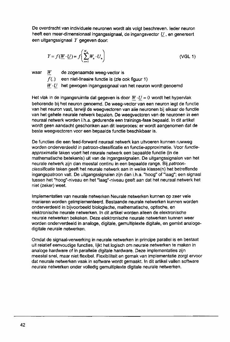
42

De overdracht van individuele neuronen wordt als voigt beschreven. leder neuron heeft een meer-dimensionaal ingangssignaal, de ingangsvector U , en genereert een uitgangssignaal Y gegeven door:

(VGL 1)

waar W de zogenaamde weeg-vector is

f(.) een niet-lineaire functie is (zie ook figuur 1)

W· U het gewogen ingangssignaal van het neuron wordt genoemd

Het vlak in de ingangsruimte dat gegeven is door W· U = 0 wordt het hypervlak behorende bij het neuron genoemd. De weeg-vector van een neuron legt de functie van het neuron vast, terwijl de weegvectoren van aile neuronen bij elkaar de functie van het gehele neurale netwerk bepalen. De weegvectoren van de neuronen in een neuraal netwerk worden i.h.a. gedurende een trainings-fase bepaald. In dit artikel wordt geen aandacht geschonken aan dit leerproces: er wordt aangenomen dat de beste weegvectoren voor een bepaalde functie beschikbaar is.

De functies die een feed-forward neuraal netwerk kan uitvoeren kunnen ruwweg worden onderverdeeld in patroon-classificatie en functie-approximatie. V~~r functie­approximatie taken voert het neurale netwerk een bepaalde functie (in de mathematische betekenis) uit van de ingangssignalen. De uitgangssignalen van het neurale netwerk zijn dan meestal continu in een bepaalde range. Bij patroon­c/assificatie taken geeft het neurale netwerk aan in welke klasse(n) het betreffende ingangspatroon valt. De uitgangssignalen zijn dan i.h.a. "hoog" of "Iaag"; een signaal tussen het "hoog"-niveau en het "Iaag"-niveau geeft aan dat het neuraal netwerk het niet (zeker) weet.

Implementaties van neurale netwerken Neurale netwerken kunnen op zeer vele manieren worden ge'implementeerd. Bestaande neurale netwerken kunnen worden onderverdeeld in bijvoorbeeld biologische, mathematische, optische, en elektronische neurale netwerken. In dit artikel worden aileen de elektronische neurale netwerken bekeken. Deze elektronische neurale netwerken kunnen weer worden onderverdeeld in analoge, digitale, gemultiplexte digitale, en gemixt analoge­digitale neurale netwerken.

Omdat de signaal-verwerking in neurale netwerken in principe parallel is en bestaat uit relatief eenvoudige functies, lijkt het logisch om neurale netwerken te maken in analoge hardware of in parallelle digitale hardware. Deze implementaties zijn meestal snel, maar niet flexibel. Flexibiliteit en gemak van implementatie zorgt ervoor dat neurale netwerken vaak in software wordt gemaakt. In dit artikel vallen software neurale netwerken onder volledig gemultiplexte digitale neurale netwerken.

Stellingen ult de literatuur Veel onderzoek op het gebied van analoge neurale netwerken wordt gemotiveerd door een aantal stellingen die in de neurale literatuur te vinden zijn. De twee meest belangrijke staan hieronder:

• the limited accuracy of analog components [for neural networks] is not a serious problem because neural networks are forgiving to component errors [5]

• for neural networks, the need for precision and for large Signal-to-Noise-Ratio is replaced by that for real-time collective processing [6]

Deze stellingen houden in dat een neuraal netwerk geen nauwkeurige hardware vereist en dat ze dUs gemaakt kunnen worden met eenvoudige en onnauwkeurige analoge circuits. De eerste stelling is juist voor zover het kleine en statische fouten betreft. De meeste fouten in ana loge elektronica zjjn echter niet statisch maar varieren continu (denk aan variaties van temperatuur en voedingsspanning, veroudering etc.). De tweede stelling is sterker dan de eerste en stelt dat ook ruis nauwelijks van belang is voor neurale netwerken. In dit artikellaten we zien dat er wei degelijk een minimum nauwkeurigheid vereist is voor een neuraal netwerk dat een bepaalde functie uitvoert. De twee (veelal geaccepteerde) geciteerde stellingen zijn dus onjuist. De in dit artikel afgeleide nauwkeurigheidseisen worden vervolgens gebruikt om te bepalen welke implementatie (analoog of digitaal) het meest vermogens-efficient is voor een bepaalde applicatie.

1.1 Opzet van het artikel

Het doel van dit artikel is het afschatten welk soort neuraal netwerk (analoog, digitaal, of mixed analoog-digitaal) het meest vermogens-efficient is voor welke klasse van applicaties. Er voigt uit de analyses dat de vermogensefficientie sterk afhangt van de applicatie. In dit artikel worden er meerdere aannames gedaan ter vereenvoudiging van de analyses. Aile aannames zijn in het voordeel van ana loge neurale netwerken; de efficientie van analoge netwerken is dus overschat. Dientengevolge is de klasse van applicaties waarvoor digitale neurale netwerken het meest efficient zijn waarschijnlijk zelts groter dan de klasse die voigt uit de analyses. Verder is er nog een tijdsaspect: met de tijd worden processen vernieuwd. Deze processen worden beter voor digitale schakelingen, maar niet voor analoge circuits. Hieruit voigt dat de klasse van applicaties waarvoor ana loge neurale netwerken het meest efficient zijn kleiner wordt met de tijd.

Aannames In de analyses wordt verondersteld dat patroon classificatie wordt gedaan; deze taak zorgt voor de laagste nauwkeurigheidseisen aan de hardware (aileen nauwkeurigheid nodig rond de classificatie-grenzen). Verder worden eenvoudige classificatietaken verondersteld, die ook weer resulteren in de laagste nauwkeurigheidseisen. Ais laatste wordt aangenomen dat het neuraal netwerk is geoptimaliseerd voor zijn taak: aile nauwkeurigheid in het systeem wordt in principe gebruikt.

43

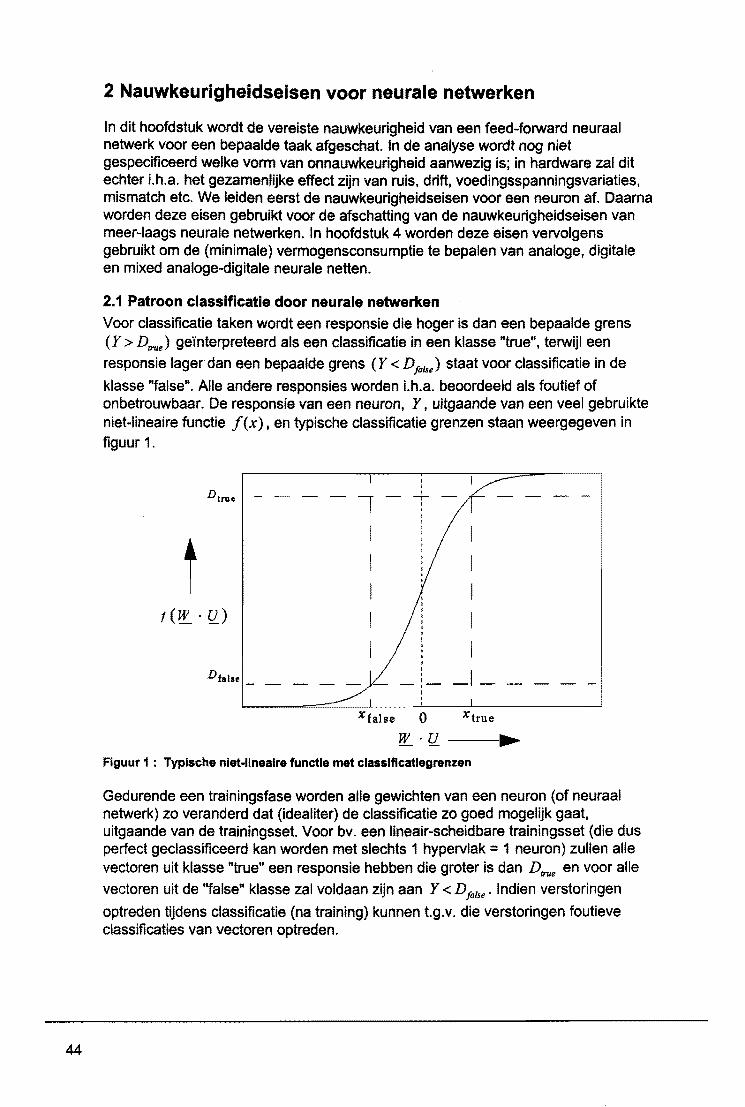
44

2 Nauwkeurigheidseisen voor neurale netwerken

In dit hoofdstuk wordt de vereiste nauwkeurigheid van een feed-forward neuraal netwerk voor een bepaalde taak afgeschat. In de analyse wordt nag niet gespecificeerd welke vorrn van onnauwkeurigheid aanwezig is; in hardware zal dit echter Lh.a. het gezamenUjke effect zijn van ruis, drift, voedingsspanningsvariaties, mismatch etc. We leiden eerst de nauwkeurigheidseisen voor een neuron af. Daama worden deze eisen gebruikt voor de afschatting van de nauwkeurigheidseisen van meer-Iaags neurale netwerken. In hoofdstuk 4 worden deze eisen vervolgens gebruikt om de (minimale) vermogensconsumptie te bepalen van analoge, digitale en mixed analoge-digitale neurale netten.

2.1 Patroon classificatle door neurale netwerken V~~r classificatie taken wordt een responsie die hoger is dan een bepaalde grens (Y> Dtrue ) ge'interpreteerd als een classificatie in een klasse "true", terwijl een responsie lager dan een bepaalde grens (Y < D false) staat voor classificatie in de

klasse "false". Aile andere responsies worden Lh.a. beoordeeld als foutief of onbetrouwbaar. De responsie van een neuron, Y, uitgaande van een veel gebruikte niet-lineaire functie f(x) , en typische classificatie grenzen staan weergegeven in figuur 1.

t DfaJse

I I I -,.-I , , I , I

-1-

Xfalse 0 Xtrue

w·u .... FIguur 1 : Typlsche nlet·llnealre functle met classlflcatlegrenzen

Gedurende een trainingsfase worden aile gewichten van een neuron (of neuraal netwerk) zo veranderd dat (idealiter) de classificatie zo goed magelijk gaat, uitgaande van de trainingsset. V~~r bv. een lineair-scheidbare trainingsset (die dus perfect geclassificeerd kan worden met slechts 1 hypervlak = 1 neuron) zullen aile vectoren uit klasse "true" een responsie hebben die groter is dan Dtrue en voor aile vectoren uit de ''false'' klasse zal voldaan zijn aan Y < Dfalse • Indien verstoringen

optreden tijdens classificatie (na training) kunnen t.g.v. die verstoringen foutieve classificaties van vectoren optreden.

Methodes voor het creiren van foutmarges

Het is evident dat indien de classificatiegrenzen gedurende trainen (D tx ) en

classificeren (DC x) identiek zijn, er geen foutmarge is. Een foutmarge kan gecreeerd worden door de grenzen tijdens trainen verder in de richting van de maximum responsie te leggen. De gecreeerde foutmarge is dan (f- 1(DCx)- f-l{Dtx»,Sign(f-l(DCx». Er zijn meerdere manieren om een dergelijke foutmarge te maken: ruis toevoegen tijdens training, vergroten van steilheid van f(x) na het trainen, etc.

2.2 Nauwkeurlgheidseisen voor enkellaags netwerken

In een hardware realisatie zijn zowel de ingangsvector U als de weegvector W onnauwkeurig. Verder zullen de sommatie en de niet-lineaire functie nog additionele fouten introduceren. Het werkelijke gewogen ingangssignaal van een neuron is dan (kleine fouten): .

(VGL 2)

waar ~naccurate en Uinaccurate de onnauwkeurigheidscomponent op Wen U zijn en

INACsum de onnauwkeurigheid is van de sommatie en van f(.)samen. Best-case komt overeen met die situatie waarvoor de eisen het lichtst zijn; voor worst-case situaties zijn de eisen het zwaarste. Een best-case afschatting van nauwkeurigheidseisen komt overeen met de situatie waarin de volledige intervallen [Dt true, DC true] en [Dt false, DC false] gebruikt worden als fout-marge 1• In dat geval is er geen effect van onnauwkeurigheid als:

n n waar W en U de maxima zijn van de gewichten en van een ingangssignaal. Ais niet voldaan is aan vgl. 3 kan de performance van het neurale net ernstig verslechteren.

Optimale nauwkeurigheldselsen

Het is optimaal als de fouten van aile bouwblokken een even grote bijdrage hebben in de overall-fout. Daarom wordt hierna aangenomen dat aile elementen in ~naccurate en in Uillaccurate eenzelfde magnitude hebben, maar verder ongecorreleerd

zijn. Dan vOigt dat:

U U ·W U inaccurate inaccurate - inaccurate fj/ n ~ n n ~ 1"\ 'VlVin

U UW U en (VGL 4)

w; ·U W; o < lIIaccurate - < inaccurate. fj/. - n 1"\ - n VlVill

WU W

1 Dil is waar voor scheidbare voorbeelden. en klopt bij goede benadering voar willekeurige sets.

45

46

waar N in gelijk is aan het aantal ingangen van het neuron.

Nauwkeurigheidseisen Combinatie van vgl. 3 en vgl. 4 levert een afschatling van de vereiste nauwkeurigheden in een neuraal netwerk dat gebruikt wordt voor classificatie. Als we een SI~ (Signal-te-Inaccuracy Ratio van het signaal x) definieren als de verhouding tussen het signaal en de onnauwkeurigheid (ruis, drift, matching, diverse verstoringen, etc.), dan voigt direct dal (worst-case):

(VGL 5)

Merk op dat de rechterkant van vgl. 5 afhangt van een aantal eigenschappen van de 1"'\ 1"'\

te classificeren set (Nin • W, U), en van de training zeit (f-'(Dt true», en van een

meestal kleine restonnauwkeurigheidsterm.

De best-case situatie zal in de praklijk niet optreden, terwijl in het algemeen vgl. 5 een te grote nauwkeurigheideis geeft. Dit is op te lossen door simpel weg voor N jn het aantal relevante ingangssignalen te nemen Lp.v. het totale aantal ingangssignalen. In het vervolg zullen we daarom uitgaan van vgl. 5.

2.3 Nauwkeurigheldselsen voor meerlaags neurale netwerken In het vorige paragraaf werden de nauwkeurigheidseisen voor losse neuronen (en dus voor enkellaags feed-forward netwerken) afgeleid. Echter, vrijwel aile bruikbare applicaties vereisen meer-Iaags neurale netwerken [2-4].

In enkellaags neurale netwerken kan de totale fout-marge gebruikt worden voor ieder neuron. In meerlaags netwerken moet de foutmarge echter verdeeld worden over meerdere gecascadeerde lag en met neuronen. De eisen per neuron in een meerlaags netwerk zijn dus hetzelfde of hoger dan de eisen aan losse neuronen (uitgaande van eenzelfde overall fout-marge). Er kan eenvoudig worden afgeleid dat een foutmarge gecreeerd kan worden door het opschalen van de helling van 1(,) na

de training met een factor, > 1 .

(VGL 6)

Voor de grootst mogelijke schaal factor (' ~ 00 ) resulteert de grootst mogelijke foutmarge. en tevens zijn dan de uitgangen van aile neuronen binair. In een meerlaags neuraal netwerk betekent dit dat de volledige foutmarge gebruikt kan worden door de eerste laag, terwijl aile volgende lagen allemaal binaire in- en uitgangssignalen hebben.

Hoewel dit soort meerlaags netwerk enige nadelen kan hebben m.b.t. classificatiemogelijkheden (voor b.v. NP·hard problemen), wordt van dit type uitgegaan omdat de nauwkeurigheidseisen het laagste zjjn: de eisen aan neuronen in het meerlaags net zijn identiek aan de eisen aan losse neuronen met overall dezelfde fout-marges.

2.4 Nauwkeurigheidseisen tegen vereiste resolutie In dit sub-hoofdstuk worden nauwkeurigheidseisen gekoppeld aan bepaalde eigenschappen van de te classificeren set: vereiste resolutie in de ingangsruimte en dimensie van de ingangsruimte. Voor de resolutie gebruiken we de volgende definitie:

De (spatia/e) resolutie E vereist voor een bepaalde classificatietaak is de minimum afstand tussen willekeurige vectoren behorende tot verschillende klassen, gerelateerd aan het maximum van een ingangssignaal:

" d (classo' class! ) = E U

Met deze definitie treedt er geen performance degradatie op t.g.v. een beperkte resolutie. Indien dit wei is toegestaan kan een beperkt gemodificeerde versie van de definitie gebruikt worden. Ais we aannemen dat de resolutie in iedere richting gehaald moet kunnen worden, dan voigt (met zowel symmetrische [(.)als

" " trainingsgrenzen) dat & W U = 2 . [-I (Dt true). Met de eerdere aannames (verwaarlozen onnauwkeurigheid van sommatie, en gelijke variantie van fouten op gewichten en ingangsignalen) voigt uit vgl. 5:

2 f2:N. SIRw ;; SIRu = SIR> V" . .LV in

& (VGL 7)

Hieruit voigt dat de eisen aan de SIR volledig bepaald worden door de uit te voeren classificatietaak: door de vereiste resolutie (&) en door de dimensie van de ingangsruimte2 (Nin )·

3 Power-consumptie voor neurale functies

In digitale neurale netwerken zijn voornamelijk veel vermenigvuldigingen en optellingen nodig Per classificatie. Voor een analoog-digitaal netwerk zijn verder AD­conversies nodig vqor ieder signaal per classificatie. In analoge neurale netwerk en zijn voornamelijk v~rmenigvuldigingen en optellingen nodig. In dit hoofdstuk wordt het vermogen afgeschat dat nodig is voor deze meest voorkomende bewerkingen. Deze worden later ;ebruikt voor de afschatting van de totale vermogensconsumptie van een neuraal netwerk.

2 De..J N/n afname van!ruis, zoals die geldt voor normale parallelle systemen treedt niet op t.g.v. het aanbieden van versclilillende signalen op de N/n ingangen.

47

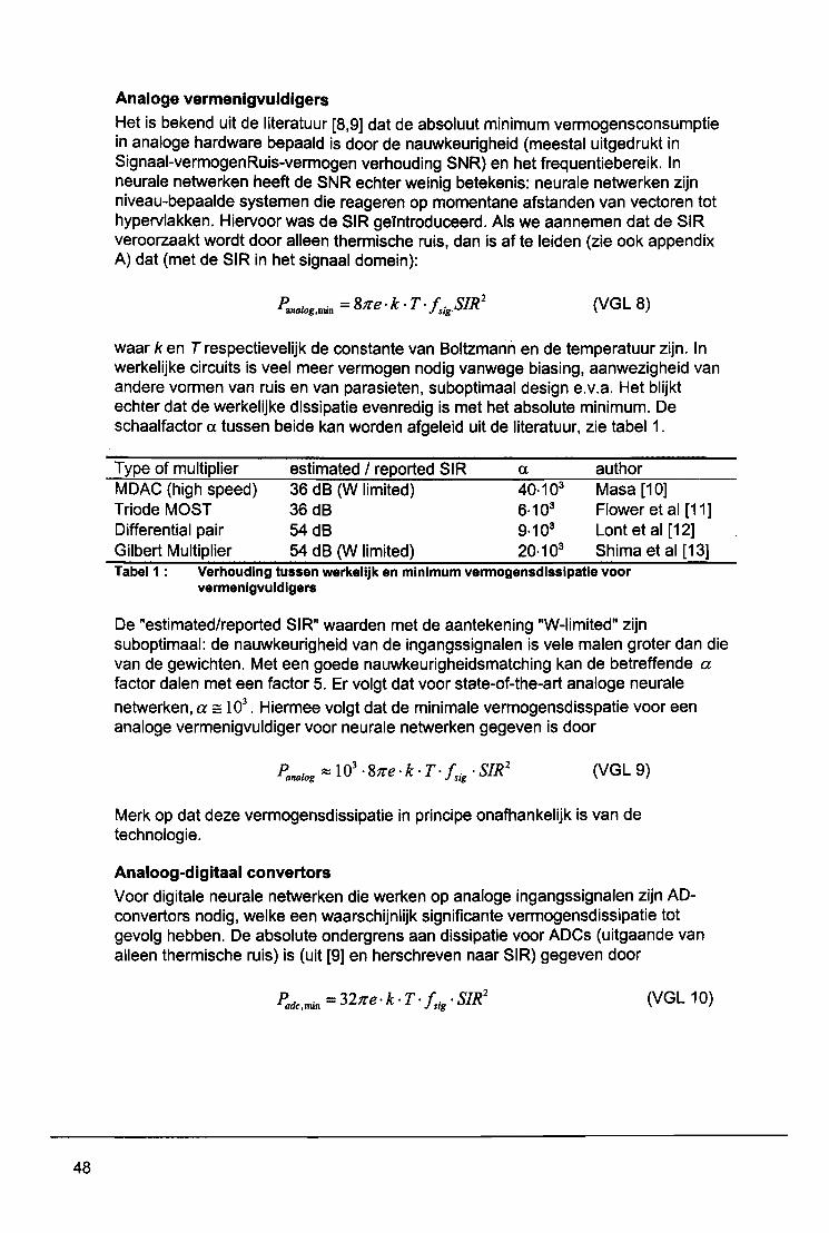
48

Analoge vermenigvuldigers

Het is bekend uit de literatuur [8,9] dat de absoluut minimum vermogensconsumptie in analoge hardware bepaald is door de nauwkeurigheid (meestal uitgedrukt in Signaal-vermogenRuis-vermogen verhouding SNR) en het frequentiebereik. In neurale netwerken heeft de SNR echter weinig betekenis: neurale netwerken zijn niveau-bepaalde systemen die reageren op momentane afstanden van vectoren tot hypervlakken. Hiervoor was de SIR ge'introduceerd. Ais we aannemen dat de SIR veroorzaakt wordt door aileen thermische ruis, dan is af te leiden (zie ook appendix A) dat (met de SIR in het signaal domein):

(VGL 8)

waar k en T respectievelijk de constante van Boltzmann en de temperatuur zijn. In werkelijke circuits is veel meer vermogen nodig vanwege biasing, aanwezigheid van andere vormen van ruis en van parasieten, suboptimaal design e.v.a. Het blijkt echter dat de werkelijke dissipatie evenredig is met het absolute minimum. De schaalfactor a tussen beide kan worden afgeleid uit de literatuur, zie tabel 1.

Type of multiplier MDAC (high speed) Triode MOST Differential pair Gilbert Multiplier

estimated / reported SIR 36 dB (W limited) 36 dB 54 dB 54 dB (W limited)

40.103

6.103

9.103

20.103

author Masa [10] Flower et al [11] Lont et al [12] Shima et al [13]

Tabel1 : Verhoudlng tussen werkelijk en minimum vermogensdlsslpatle voor vermenlgvuldlgers

De "estimated/reported SIR" waarden met de aantekening "W-limited" zijn suboptimaal: de nauwkeurigheid van de ingangssignalen is vele malen groter dan die van de gewichten. Met een goede nauwkeurigheidsmatching kan de betreffende a factor dalen met een factor 5. Er voigt dat voor state-of-the-art analoge neurale

netwerken, a == 103• Hiermee voigt dat de minimale vermogensdisspatie voor een

analoge vermenigvuldiger v~~r neurale netwerken gegeven is door

~nalog ~ 103 • 81l'e . k . T· f'sig • SIR 2 (VGL 9)

Merk op dat deze vermogensdissipatie in principe onafhankelijk is van de technologie.

Analoog-digitaal convertors Voor digitale neurale netwerken die werken op analoge ingangssignalen zijn AD­convertors nodig, welke een waarschijnlijk significante vermogensdissipatie tot gevolg hebben. De absolute ondergrens aan dissipatie voor ADCs (uitgaande van aileen thermische ruis) is (uit [9] en herschreven naar SIR) gegeven door

~dc.min = 321l'e' k . T . f'sig • SIR2 (VGL 10)

Voor ADCs die in dissipatie door therrnische ruis begrensd zijn (CMOS U ADCs), is de werkelijke dissipatie bij goede benadering Padc = p. Padc,min' Dit zijn meestal hoge

resolutie (12b(bits)-18b) ADCs voor signalen in de audio-band. Voor hoge-snelheid ADCs (met een gelimiteerde nauwkeurigheid: <12b). worden vele verschillende architecturen gebruikt. Elke heeft voor zijn speci'fieke applicatie minimale verrnogensdissipatie of oppervlaktegebruik. Het blijkt dat de praktische dissipatie voor hoge-snelheid ADCs vrijwel constant is voor resoluties tot 12b. Een goede fit over vele state-of-the-art CMOS ADCs [13-19] geeft:

(VGL 11)

waar 4rdc == 1.10-15• Bade == 2.10-9

hig de maximum frequentie van het ingangssignaal is (vgls. Nyquist)

De hoge resolutie ADCs in vgl. 11 kunnen niet werken op hoge frequenties. Ais geen hoge conversiefrequenties nodig zijn, kunnen CMOS LA ADCs worden toegepast voor vrijwel iedere resolutie. In dat geval wordt de werkelijke dissipatie gegeven door

(VGL 12)

ADCs in niet-CMOS processen kunnen een lagere dissipatie hebben, terwijl ontwerp­slimheid en proces-ontwikkeling ook de dissipatie kunnen veranderen.

Digitale vermenigvuldigers

Voor digita/e signaalverwerking is de dissipatie athankelijk van het aantal bits, de klokfrequentie en van twee varia belen die athangen van het type circuit en van de technologie [20]:

(VGL 13)

waar: E/r is de energie per transitie van een gate (technologie ath.) ielock is de vermenigvuldigingsfrequentie Sscale bevat de waarschijnlijkheid op een gate-omslag en bevat het aantal

gates nodig voor een elementaire opera tie

Typische getallen voor de schaalfactor Sscale' n2 kunnen weer gevonden worden in

de literatuur [8,20-22]; ze vari~ren van 50· n2 tot < 2n2 • Hierrnee kan vgl. 13

orngeschreven worden voor neurale bewerkingen; met een onnauwkeurigheid geUjk aan 1/2 LSB en met een bepaalde rond 0 symmetrische gewichtsrange voigt dan:

waar: SIR

fxl

20·1og(SIR) (r ]2

~ig = 2 . Sscale • hir . 6 . E/r (VGL 14)

is de vereiste SIR (aileen afrondfouten in aanmerking genomen) afrondt naar het dichtstbijzijnde gratere gehele getal

hir is de signaal frequentie Multiplexen van digitale functies vermindert de dissipatie norrnaliter niet.

49

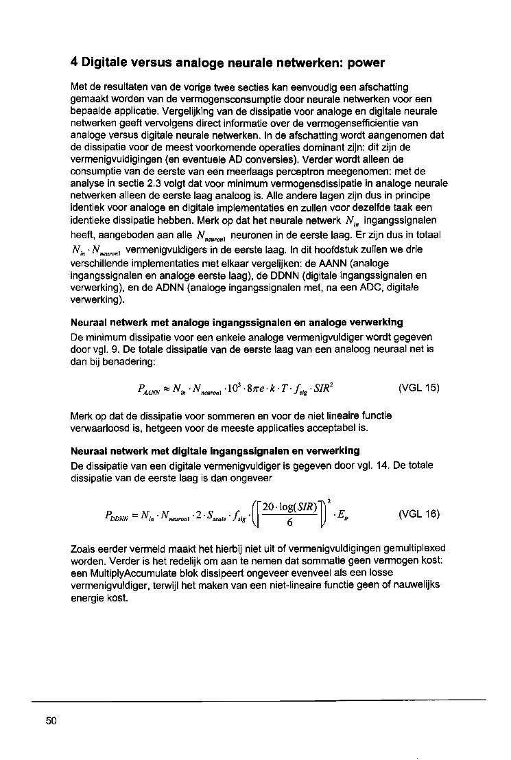
50

4 Digitale versus analoge neurale netwerken: power

Met de resultaten van de vorige twee secties kan eenvoudig een afschatting gemaakt worden van de vermogensconsumptie door neurale netwerken voor een bepaalde applicatie. Vergelijking van de dissipatie v~~r analoge en digitale neurale netwerken geeft vervolgens direct informatie over de vermogensefficientie van analoge versus digitale neurale netwerken. In de afschatting wordt aangenomen dat de dissipatie voor de meest voorkomende operaties dominant zijn: dit zijn de vermenigvuldigingen (en eventuele AD conversies). Verder wordt aileen de consumptie van de eerste van een meerlaags perceptron meegenomen: met de analyse in sectie 2.3 voigt dat voor minimum vermogensdissipatie in analoge neurale netwerken aileen de eerste laag analoog is. Aile andere lagen zijn dus in principe identiek voor analoge en digitale implementaties en zullen voor dezelfde taak een identieke dissipatie hebben. Merk op dat het neurale netwerk N in ingangssignalen

heeft, aangeboden aan aile Nneuronl neuronen in de eerste laag. Er zijn dus in totaal

N in . Nneuronl vermenigvuldigers in de eerste laag. In dit hoofdstuk zullen we drie verschillende implementaties met elkaar vergeHjken: de AANN (ana loge ingangssignalen en analoge eerste laag), de DONN (digitale ingangssignalen en verwerking), en de ADNN (analoge ingangssignalen met, na een ADC, digitale verwerking).

Neuraal netwerk met analoge ingangssignalen en analoge verwerking De minimum dissipatie voor een enkele analoge vermenigvuldiger wordt gegeven door vgl. 9. De totale dissipatie van de eerste laag van een analoog neuraal net is dan bij benadering:

Merk op dat de dissipatie voor sommeren en voor de niet lineaire functie verwaarloosd is, hetgeen voor de meeste applicaties acceptabel is.

Neuraal netwerk met digitale ingangssignalen en verwerking

(VGL 15)

De dissipatie van een digitale vermenigvuldiger is gegeven door vgl. 14. De totale dissipatie van de eerste laag is dan ongeveer

=. .. . . 20 ·log(SIR) . E (I 1)2

PDDNN N in Nneuronl 2 Sscale hig 6 tr (VGL 16)

Zoals eerder vermeld maakt het hierbij niet uit of vermenigvuldigingen gemultiplexed worden. Verder is het redelijk om aan te nemen dat sommatie geen vermogen kost: een MultiplyAccumulate blok dissipeert ongeveer evenveel als een losse vermenigvuldiger, terwijl het maken van een niet-lineaire functie geen of nauwelijks energie kost.

Neuraal netwerk met analoge ingangen en digitale verwerking

Voor neurale netwerken met analoge ingangen en digitale verwerking, is vermogen nodig voor zowel AD-conversies als voor de digitale verwerking. De totale dissipatie is dan

P _ N . N . (p ~dc '1 ADNN '" in neuron 1 dig + N I

neuron1 J (VGL 17)

Afhankelijk van de conversiefrequentie moet ofwel vgl. 11 of vgl. 12 gebruikt worden.

Een iIIustratie

In figuur 2 staat de vermogensconsumptie van een neuraal netwerk als functie van de SIR, voor zowel de AANN, de ADNN als de DONN implementatie. Merk op dat de dissipatie geschaald is naar het aantal vermenigvuldigers en de signaalfrequentie. Voor de ADNN is verder het aantal neuronen van belang; curven zijn getekend voor Nneuronl = 10 en voor Nneuronl == 100. De signaalfrequentie bepaalt tevens het type ADC dat gebruikt kan worden in een ADNN; figuur 2a geeft de laag-frequent situatie weer terwijl figuur 2b het hoogfrequent geval laat zien. V~~r de berekeningen is uitgegaan van een modern 0.5 Jlm CMOS proces.

,~" 1

+ , .. , 1

I ",'.: 1 . DONN

~ ~ I~ U$U ~-I--, "'--,..........~--,r-~--,-----,--I

SlR (dB) .... SlR (dB) --....

Figuur 2 : Geschatte vermogensdissipatie (genormeerd) voor neurale netten als functie van SIR: (a) laag midden frequent (b) hoog frequent

Er voigt dat een analoog neuraal netwerk vermogensefficienter is dan een digitaal neuraal netwerk voor applicaties die kunnen volstaan met een lage SIR. Verder blijkt dat een ADNN aileen efficienter is dan een AANN als er voldoende neuronen in de eerste laag zijn. Ten gevolge van proces-evolutie zal digitale processing efficienter worden [7], terwijl ana loge processing op zijn best niet verslechtert. Dientengevolge zal het break-even punt tussen de AANN en de DONI\! over tien jaar gedaald zijn van de huidige 50dB naar ongeveer 30dB. Samen met vgl. 7 kan nu afgeschat worden voor welke applicaties welk type implementatie het meest vermogensefficient is.

4.1 Vermogens-efficiente neurale netwerken

Combinatie van vgl. 7, 15, 16 en 17 levert direct een figuur waarin als functie van erg elementaire eigenschappen van een te classificeren set (nl. de vereiste resolutie en de dimensie van de ingangsvectoren) de meest vermogens-efficiente implementatie staat. Met de verwachte evolutie van CMOS processen [7] kan in deze figuur het verloop in de tijd worden uitgezet.

51

52

.0

t .oo~, I e

IO.Om

10m

00

. . (power. 2(06) useful AANN applicatIOns • 1 "'M1IN,,,~'''''''M g use (power. 1996-2()(J6)

E

v------ADNN and DDNN !!pJllieations (power, 1996)

'.0 .00

1.5.0

Nln--~

1<)0

S]R=30dB

iJ S]R=50dB +1

1>0

Figuur 3 : Applicatie ruimte van neurale netten (vereiste resolutie en ingangsdimensie), en onderverdeling op grond van vermogensdissipatie, inclusief tijdextrapolatie

Merk op dat de afschattingen van vermagensdissipatie enige mate van onnauwkeurigheid hebben. Dit heeft echter geen significante impact op de resultaten in 'figuur 3: als de vermogensafschatting er bv. 3dB naast zit veranderen de jaartallen in de figuur met slechts 1 jaar. Verder zijn gedurende de analyse vele aannames gemaakt in het voordeel van analage implementaties; in werkelijkheid zal niet altijd aan al deze aannames voldaan zijn. Dit houdt in dat de efficientie van analoge neurale netwerk en t.o.v. digitale implementaties in werkelijkheid lager is dan die in figuur 3.

5 Conclusies

Dit artikel laat zien dat nauwkeurigheidseisen aan (feed-forward) neurale netwerken kunnen worden afgeleid en dat deze eisen afhangen van een paar elementaire eigenschappen van de applicatie. Deze eisen zijn gebruikt om een afschatting te maken van het benodigde vermogen voor een analoog, digitaal en mixed-analoog­digitaal neuraal netwerk. Uit de afschatting voigt dat analoge neurale netwerken meer vermogens-efficient zijn dan digitale als:

• het aantal eerste-/aag neuronen klein is (typisch < 10) en de ingangssignalen ana/oog zijn

• lage spatiele resolutie getolereerd kan worden voor de applicatie Op dit moment (3.3V 0.5~m CMOS proces), ligt de grens bij 1 % resolutie. Door processevolutie stijgt deze grens naar ca. 10% in het jaar 2007.

Voor aile andere applicaties zijn djgitale neurale netwerken efficienter m.b.t. vermogensconsumptie. In de analyses zijn een aantal aannames gemaakt in het voordeel van analoge neurale netwerken, het is dus waarschijnlijk dat de werkelijke efficientie van ana loge netten lager is.

6 References

[1] A.J.Annema, F.P.Widdershoven, and B.Nauta, "Neural Networks: Analog versus Digital Hardware", submitted to IEEE Circuits and Systems

[2] D.E.Rumelhart, G.E.Hinton and R.J.Williams, "Learning internal representations by error propagation", in Parallel Distributed Processing, vol. 1, chapter 8, eds. D.E.Rumelhart and J.LMcCleliand, Cambridge, MA: MIT Press, 1986

[3] RP.Lippmann, "An Introduction into Computing with Neural Nets", IEEE ASSP Mag, vol. 4, pp. 4-22, 1987

[4] A.J.Annema, "Feed-Forward Neural Networks: Vector Decomposition Analysis, Modelling and Analog Implementation", Norwell MA: Kluwer Academic Publishers, 1995

[5] J.van der Spiegel, P .Mueller, D.Blackman, P .Chance, C.Donham, REtienne­Cummings, and P.Kinget, "An Analog Neural Computer with Modular Architecture for Real-Time Dynamic Computations", IEEE JSSC, vol. 27, Jan 1992, pp. 82-92

[6] E.Vittoz, "Analog VLSI for Advanced Signal Processing", in Proc. Workshop on Future Information Processing Technologies, Helsinki, Sept 4-8, 1995

[7] IEEE Spectrum, Technology 1996 Analysis and Forecast Issue, pp. 51-55, Jan. 1996

[8] E.A.Vittoz, "Low-Power Design: Ways to Approach the Limits", in IEEE International Solid-State Circuits Conference, Dig. Paper, 1994, pp. 14-18

[9] E.Dijkstra, O.Nys, E.Blumenkrantz, "Low Power Oversampled AID Con verters", in "Analog Circuit Design", eds. RJ. vd Plassche, W .Sansen, and J.H.Huijsing, Kluwer Academic Publishers, 1995

[10] P.Masa, "NeuroClassifier", Ph.D. thesis, Twente University, The Netherlands, 1994

[11] B.Flower and M.Jabri, "The implementation of Single and Dual Transistor VLSI Synapses", Proc. Third Symposium on MicroNeuro, Edinburgh, Scotland, 1993, pp. 1-10

[12] J.B.Lont and W.Guggenbuhl, "Analog CMOS Implementation of a Multilayer Perceptron with Nonlinear Synapses", IEEE Tr. Neural Networks, vol. 3, 1992, pp.457-465

[13] T.Shima, T.Kimura, Kamatani, T.ltakura, Y.Fujita, and T.Lida, "Neuro Chips with On Chip Back-Propagation and/or Hebbian Leaming", IEEE JSSC, 1992, pp. 1868-1875

53

54

[14J S.Tsukamoto, I.Dedic, T .Endo, K.Kikuta, K.Goto, and O.Kobayashi, " A CMOS 6b 200MSample/s 3V-Supply AID Converter for a PRML Read Channel LSI", in IEEE International Solid-State Circuits Conference, Dig. Paper, 1996, pp. 70-71

[15] A.G.W.Venes and R.J. van de Plassche, " An 80MHz 80mW 8b CMOS Folding AID Converter with Distributed T/H Preprocessing", in IEEE International Solid­State Circuits Conference, Dig. Paper, 1996, pp. 318-319

[16] M.Yotsuyanagi, H.Hasegawa, M.Yamaguchi, M.lshida, and K.Sone, "A 2V, 10b, 20Msample/s, Mixed-Mode Subranging CMOS AID Converter", IEEE J. Solid-State Circuits, vol. 30, December 1995, pp. 1533-1537

[17] P.C.Yu, H.S.Lee, "A 2.5V 12b 5MSample/s Pipelined CMOS ADC", in IEEE International Solid-State Circuits Conference, Dig. Paper, 1996, pp. 314-315

[18] E.J.vd Zwan, and E.C.Dijkmans, "A 210 micro W CMOS SigmaDelta AID Converter for Speech Coding with 80 dB Dynamic Range", IEEE ISSCC, 1996, pp.232-233

[19] P. van Gog, B.M.J.Kup, and R.van Osch, "A Two-Channel 16118b Audio AD/DA Including Filter Function with 60/40mW Power Consumption at 2.7V", IEEE International Solid-State Circuits Conference, 1996, pp. 208-209

[20] E.A.Vittoz, "Future of Analog in the VLSI Environment", in Proc. IEEE ISCAS, pp. 1372-1375, 1990

[21] J.A.J.Leijten, J.L.Meerbergen, and J.van Jess, "Analysis and Reduction of Glitches in Synchronous Networks", in Proc. ED&TC, pp. 398-403,1995

[22] T.Sakuta, W.Lee and P.Balsara, "Delay Ballanced Multipliers for Low 5:45 Power/Low Voltage DSP Core", Symp. on Low Power Electronics, Dig. Tech. Pap., pp. 36-37, 1995

[23] D.Slepian, Key Papers in the Development of Information Theory, IEEE Press: 1974

Appendix A Vermogen limiet voor analoge neurale netwerken

In deze appendix wordt de absolute ondergrens aan vermogensdissipatie voor niveau-bepaalde analoge systemen (ana loge neurale netwerken) afgeleid. Voor deze afleiding wordt uitgegaan van aileen thermische ruis. Ais we aannemen dat aileen het niveau van de signalen informatie bevat (als hypervlakken worden gebruikt voor een functie), dan is het grootst mogelijke signaal een RTS (random telegraph signal) signaal met amplitude gelijk aan de halve voedingsspanning. Het vermogen dat nodig is om dit signaal op een capaciteit te zetten is

(VGL 18)

waar: C de capaciteitswaarde is, hig de signaalsfrequentie is, VB de

voedingsspanning is, en Vpp de piek-piek waarde van het signaal is.

Het thermische ruisvermogen over de capaciteit is [11]:

2 k·T v noise =

C (VGL 19)

Het verband tussen een thermisch ruisniveau en de onnauwkeurigheidsterm in de SIR kan worden afgeleid uit de informatie theorie [23]. Er voigt dat het aantal effectieve bits in een signaal S met resolutie res is

N ejJ =2Iog(res) - I ~ .2Iog(~)=21og(SIR) (VGL 20)

waar ~ de waarschijnlljkheid is dat de waarde van het signaal in een ander quantisatieniveau valt door aileen ruis. Voor thermische ruis levert dit:

2 2 ( V pp ) Vpp [# 1 NejJ == loge SIR)~ log M:::: ~ SIR ~ - . -k . M::::

0'·v2lre 2 T v2lre (VGL 21)

waar: 0' de effectieve waarde van de ruis is.

Hieruit voigt dat voor neurale netwerken de ~2lre. 0' waarde van de thermische ruis correspondeert met de onnauwkeurigheid van de ruis. Combinatie van vgl. 18-21 levert dan de volgende relatie tussen minimum vermogensdissipatie nodig voor een bepaalde SIR:

2 VB p= 8lre·k·T· 1', ·SIR .-lSlg V

pp

Merk op dat als de SIR-eis vertienvoudigt, het minimale vermogen dan verhonderdvoudigt.

(VGL 22)

55

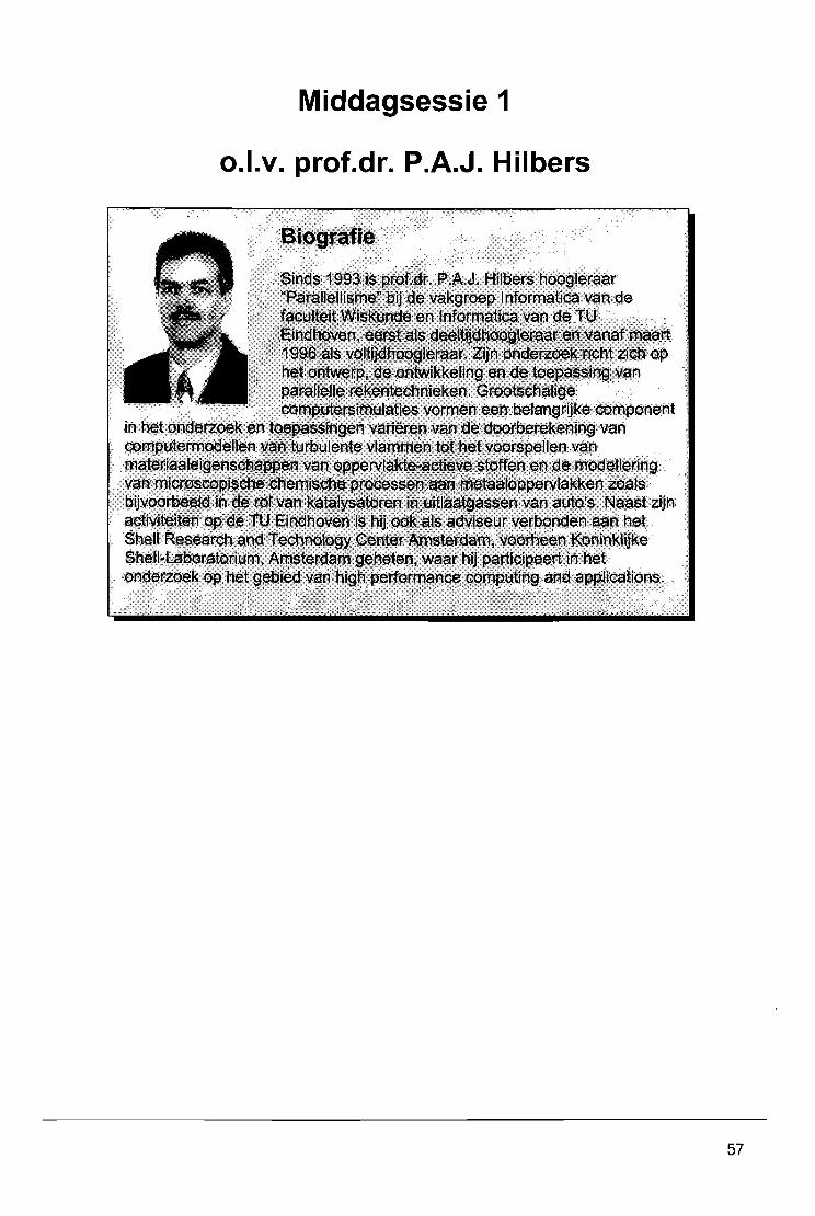
Middagsessie 1

o.l.v. prof.dr. P .A.J. Hilbers

Biegrafie

Sinds 1993 isprof'~f. P.A;J. Hilbers hoogleraar "Parallellisme" bij.de vakgroep Informatica van de tacu1tf!it WlskuNtte en Informatica van !iie"tU eind~ven.· alsdeeltljdl1<;lQ:Qt~.afen vanaf maart 199a~els vo: Ilera,ar. ZiJn<i>n€lerzoek richt zidl GcP hetontwerp. de;;.ot!lwikkeling en de toepa$Sing van paFallelle rekentethnieken. GrootschaJiie computersimulatles vormen een beJangFrjkecomponent

in het onderzoeken t0epat>singen varieren van' de· d00rberekening Van computermodellen, van turbulente vlammen tot het voorspellen van mate'fiaaleigensotapp~rtvan (l),pervlakte~actie",e, ~taffenen de modellering van"miCr(f):scoQi~che(ehemiSdfle procesSert;fa~l1I!_t~aloppervlakken zoals bijvoo~e'dio€le ,r"l van katalysatoren i~Jtlrl~~~!assen van auto's. Naast zijn actMteiteFl op de tUEindhoven is hiJ odRals adviseur verbonden aan hat Shell Resear<:h and Technology Genter .Amsterdam, voerheen Koninklijke Shell-laberatorium, Amsterdam geheteh, waar hij participaert in hat onderzeek op het gebled van hig~. performance com~lJtifl§"aflJtjaj1).ji)jlcations.

57

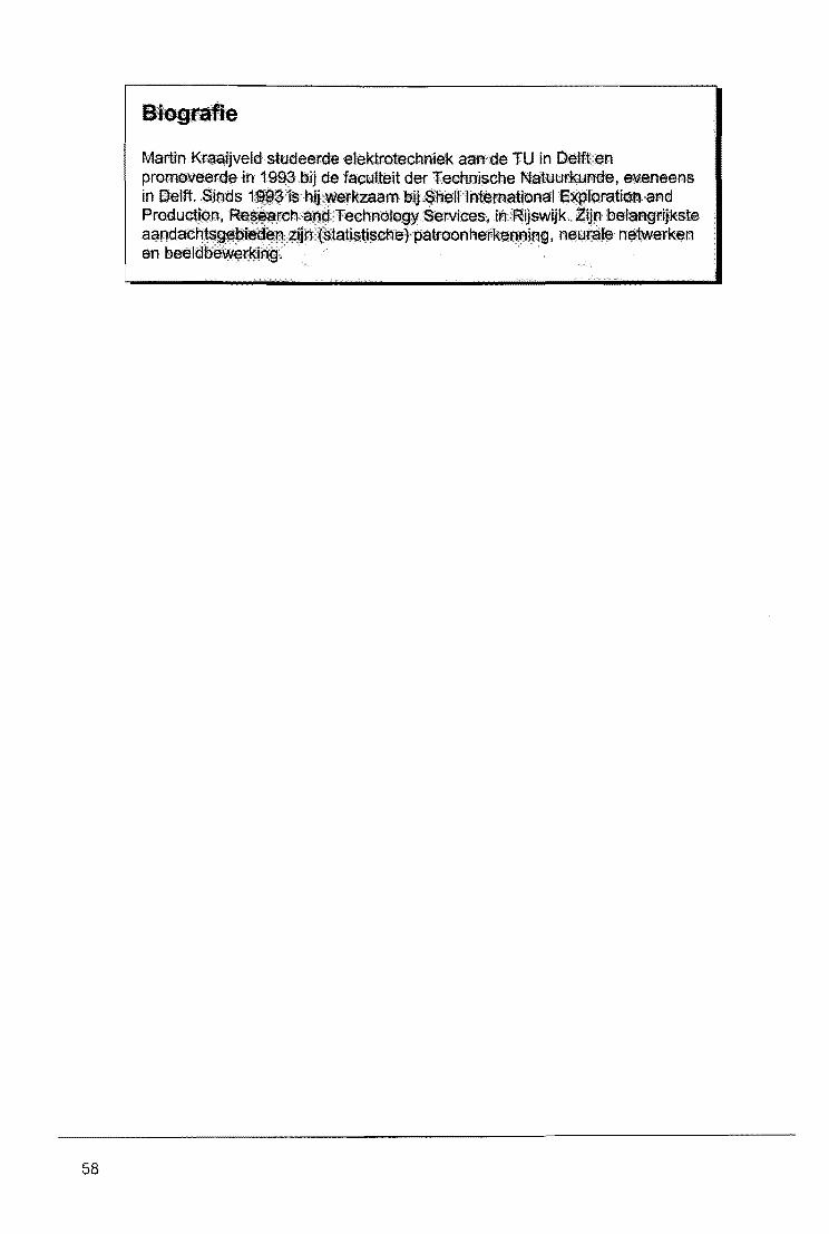
58

Martin Kfa'aijveld studeerde elektrotechniek a81'l: de TU in Delft en prornoveerdein 1993 bij de faculteit der Technischej\jJa~urktrnae, eveneens in Delft. Sinds 1993 ishijwerkzaambij Shell InteF~QnalExploratiCffl anal P'reduction, Researcha:n(ll'€chnology Services, .iJ!lRijswijk. Zijn belangrijkste aafldachtsgebieden zijn (statistische) patroonhem'S'l"Il'1ing, neurale netwerken en beeldbewerking.

Onderzoek en Toepassingen van Neurale Netwerken bij Shell

Martin A. Kraaijveld, Willem J.M. Epping & Guozhong An Shell EPT

P.O. Box 60 2280 AB Rijswijk

e-mail: m.a.kraaijveld@siep.shell.com

Sinds de hemieuwde wereldwijde belangstelling voor neurale netwerken in de tachtiger jaren. heeft Shell veel onderzoek op het gebied van neurale netwerken verricht. In eerste instantie spitste dit werk zich toe op haalbaarheidsstudies, waarbij de bruikbaarheid van neurale netwerken voor diverse toepassingen werd beoordeeld. Hierbij werden de prestaties van neurale netwerken veelal afgemeten aan de methoden die in de praktijk voor deze toepassingen gebruikt werden. Later ontstond de behoefte meer inzicht te verkrijgen in de sterke en zwakke kanten van neurale netwerken, hetgeen geleid heeft tot meer theoretisch gericht onderzoek. Een aantal voorbeelden van het werk dat in de loop der jaren bij Shell verricht is, is het volgeride:

• De herkenning van gesteente type uit wireline logs [1]. Wanneer een put geboord is worden een aantal meetinstrumenten neergelaten die diverse fysische parameters als functie van de diepte registreren. Op grond van deze metingen is het mogelijk voorspellingen te doen van de porositeit van het gesteente, de permeabiliteit, het type gesteente (zand. klei, schalie, steenkool, etc.), en de aanwezigheid van olie en/of gas. De herkenning van het gesteente type is een probleem dat momenteel met veel succes door neurale netwerken wordt opgelost.

• Het herkennen van "firstarrivals" in seismiek [2]. Een uitermate belangrijke bron van informatie voor het opsporen van olie en/of gasvoorraden is seismisch onderzoek. Hierbij wordt de structuur van de eerste paar kilometer van de aardkorst afgebeeld door middel van metingen van gereflecteerde akoestische energie. Voor een correcte afbeelding is het van belang de reflecties van diepere lagen te scheiden van de golf die zich met relatief lage snelheid via het aardoppervlak voortplant. Neurale netwerken blijken hierbij een belangrijke rol te kunnen spelen.

• Een theoretisch model voor het toevoegen van ruis bij de training van neurale netwerken [3]. Uit empirisch onderzoek was eerder gebleken dat het toevoegen van ruis, hetzij aan de trainingsdata, hetzij aan de gewichten van het netwerk, tot een verbetering van de prestaties van het neurale netwerk leidt. Door middel van theoretisch werk (o.a. op het gebied van de regularisatie theorie) is aangetoond waarom dit het geval is.

59

60

• Een patroonherkenningsmethode die robuust is bij kleine verschillen tussen de trainingsdata en de testdata [4]. Indien de statistische eigenschappen van de data waarmee het netwerk getraind is afwijken van de eigenschappen van de data die het netwerk later classificeert zal het netwerk niet optimaal presteren. De beschreven methode is in staat om te anticiperen op beperkte afwijkingen van training en test data.

Referenties

[1] Epping, W.J.M., Oudshoff, S.M., and Abbots, F.V., "Lithofacies Identification from Wireline Logs", Proc. of the International Conf. on Artificial Neural Networks, Amsterdam, The Netherlands, Sept. 13 16, 1993, 876 881.

[2] An G., and Epping, W.J.M, "Seismic firstarrival picking using neural networks", Proc. of the World Congress on Neural Networks (WCNN'93, Portland), volume I, Hillsdale, NJ, 1993. LEA.

[3] An. G., "The effects of adding noise during backpropagation training on generalization performance", Neural Computation , 8:643674, 1996.

[4] Kraaijveld, M.A., "A Parzen Classifier with an Improved Robustness against Deviations of Training and Test data", Pattern Recognion Letters, Vol. 17, 1996, pp. 679 689.

Techniek. wetenscllap en de kracht van

MA TLAB sot1ware voor technische vraagstukken. Grafisch en interactief, sne\, nauwkeurig en mtultief.

MA TLAB heeft een open structuur waar sot1ware modules met uw eigen software gekoppeJd kunnen worden. Maak gebruik van standaard functies voar mathematica, mechanica, meet & rcgeltechniek, en grafische weergave. Er zijn kant en klare modules voor specifieke toepassingen: geen losse programma's meer en vee! minder eigen programmeerwerk!

+

MATLAB

l Niet-destroc/jej ollderzoek bij McDonnell Douglas door middel van ulft'asaon ofUlerzoek. in combinatie met MATLAR. V oorbeeld; Longbow Apache helicopter

MA TLAB omvat numerieke berekingen, visualisatie en een eigen programmeer­taal. MA TLAB heeft meer dan 500 technische, mathematische en weten­schappelijke routines, die geschreven zijn door experts.

Wilt U meer weten over MATLAB? Vraag een gratis brochure aan bij:

SCIENTIFIC .OFTWARE

Bleulandweg 1B 2803 HG Gouda Tel: 0182 - 53 7644 Fax: 0182 - 570380 Email: info@ssb.nl

U kunt er jaren over doen om een nieuwe techniek onder de knieen te krijgen. Of u kunt het in een paar dagen doen in samenwerking met iemand die die jaren al ge'investeerd heeft.

BIOLOGICA BIOlOGICA heeft al jaren ervaring met tal van soorten toepassingen van kunstmatige neurale netwerken en is niet bang voor nieuwe avonturen.

V~~r meer informatie:

telefoon: fax: email: postadres:

0318-413954 0318-413944 egberts@biologica.nl Julianalaan 35, 6721 ED Bennekom

62

D.J.N. Egberts heeft in biologie en filosofie gestudeerd. Na een onderzoek aan de Rijksuniversiteit te het biotechnologisch bedrijf Holland Biotech . . gedaan te hebben heeft hij de.overstap gemaaki haar de wereld van de

: kunstmatige intelligentie. AanvankeliJk werkte hij in

loondienst voornamelijk aan Expert Systemen, en . opgerichte bedrijf BIOLOGICA \lnr,rn:;;o

Kunstmatige Neurale. Netwerken. met

Kunstmatige neurale netwerken in de financiele dienstverlening

Inleiding

D.J.N. Egberts, Biologica, Bennekom egberts@biologica.nl

In de financiele wereld wordt men geconfronteerd met de paradoxale toestand dat er tegelijkertijd voldaan moet worden aan de strengste eisen van nauwgezetheid en reproduceerbaarheid aan de ene kant, en aan de andere kant, dat winsten aileen gemaakt kunnen worden door optimaal gebruik te maken van de vage en

. irreproduceerbare aspecten van de materie waar men mee werkt.

Nauwgezet en reproduceerbaar moet men bijvoorbeeld zijn in de boekhouding en het nakomen van beloften aan klanten. Maar hiermee is nauwelijks winst te maken. De grote winst wordt gemaakt door zo goed mogelijk gebruik te maken van de grilligheid van de (menselijke) natuur en de hiervan afgeleide financiele markten. Ais bijvoorbeeld al van tevoren exact vast te stellen is wanneer er een aardbeving zal plaats' vinden en hoe groot de aangerichte schade zal zijn heeft het geen enkele zin een verzekering hiertegen aan te bieden. Daar zal niets aan verdiend kunnen worden. Verdiend kan er door een verzekeringsmaatschappij worden als iedereen denkt dat er een aardbeving komt, en dus graag een verzekering afsluit tegen de gevolgen, zonder dat die aardbeving ook echt optreedt. Verdiend kan er bijvoorbeeld ook worden aan een levensverzekering waar de verzekerde geen gebruik van zal maken omdat hij of zij overlijdt voor de uitkeringsdatum. De premie is in deze gevallen de winst. In werkelijkheid gaat het hierbij om de kans dat die aardbeving op zal treden of de geschatte leeftijd die mensen kunnen bereiken. Statistiek is dan ook een van de belangrijkste hulpmiddelen in de financiele wereld.

De mogelijkheden die de ontwikkelingen in de informatietechnologie boden met betrekking tot nauwgezet en reproduceerbaar werken werden al heel snel onderkend door banken en verzekeringsmaatschappijen. Maar ook waren zij de eersten die de mogelijkheden van kunstmatige neurale netwerken onderkenden om om te gaan met onzekere en incomplete kennis. In deze voordracht wi! ik laten zien welke problemen zoal met vrucht aangepakt kunnen worden met kunstmatige neurale netwerken. Ik zal dit iIIustreren met enkele voorbeelden van gepubliceerde toepassingen.

63

64

Toepassingen

Aile toepassingen van neurale netten in de financiele wereld draaien om de begrippen optimaliseren en voorspellen. Een toepassing waarbij beide begrippen verenigd worden is een systeem dat de hoeveelheid geld bepaalt die per dag in een geldautomaat gedaan moet worden (Bowen en Bowen, 1990). Oit mag niet te veel zijn (kost rente) en niet te weinig (dan lopen de klanten weg). Een neuraal net dat getraind is met historische gegevens over allerlei omstandigheden (weer, dag van de week, feesten, etc.) en de daarbij uit de automaat opgenomen hoeveelheid geld geeft de optimale lading aan. Bowen en Bowen vergeleken een neuraal netwerk met een expert systeem en een menselijke expert. In de hier beschreven resultaten leverde de expert het beste resultaat, het neurale net de volgende en het expert systeem de slechtste. In deze toepassing werd gebruik gemaakt van een Backpropagation Netwerk. Oit is verreweg het meest gebruikte netwerkalgorithme. Ongeveer 95% van aile gepubliceerde toepassingen wordt gedaan met Backpropagation Netwerken, ongeveer 3% met een Kohonen Netwerk en ongeveer 2% met een ander algorithme (bijvoorbeeld een Hopfield Netwerk).

De volgende toepassingen geven ongeveer aan hoe breed de inzetbaarheid van neurale netten is.

Database mining

Bedrjjven en andere instellingen hebben gegevensbestanden die vol met gegevens zitten waar veel meer informatie uit gehaald zou kunnen worden dan nu vaak gebeurt. Kunstmatige neurale netwerken kunnen helpen verbanden te vinden die we zelf zo maar niet zouden zien, doordat ze in staat zijn zonder vermoeid of verveeld te worden een bestand te onderzoeken op het optreden van bepaalde patronen (Grupe en Owrang, 1995).

Analyseren en voorspellen van de levensvatbaarheid van een bedrijf

Tot een van de taken van de accountant behoort het tijdig waarschuwen wanneer een bedrijf een vergroot risico loopt in fianciele moeilijkheden te komen. Oit is een ingewikkelde taak waarbij grote belangen op het spel staan. Er worden tal van onderzoeken gedaan met statistische methoden, en de laatste tijd wordt hierbij ook gekeken naar neurale netten (Lenard et aI., 1995).

In Spanje heeft SerranoCinca (1996) het nut van een unsupervised (Kohonen) netwerk onderzocht bij het bepalen van de verwachting volgens welke een bank failliet zou kunnen gaan. De resultaten met de neurale netwerktechniek werden vergeleken met die welke verkregen werden met andere statistische technieken (zoals lineaire discriminant analyse) en backpropagation neurale netwerken. Hij ontwikkelde een systeem dat verschillende technieken combineert en dat heel bruikbare resultaten oplevert.

Hetzelfde probleem werd door Wilson en Sharda (1994) aangepakt, ook voor een vergelijkend onderzoek tussen discriminant analyse en backpropagation neurale netwerken. Ook zjj vonden dat de resultaten met neurale netwerken de betere waren.

Voorspellen van beurs en valutakoersen

Donaldson en Kamstra (1996) vergeleken neurale netten en andere statistische technieken bij het maken van gecombineerde tijdreeks voorspellingen van de koersgevoeligheid op verschillende beurzen en vonden dat de resultaten met neurale netwerken superieur waren aan die welke met andere technieken bereikt werden.

Prijscalcu latie

Een bedrijf dat produkten maakt die steeds wei op elkaar lijken, maar nooit precies hetzelfde zijn heeft soms een probleem bij het bepalen van de produktiekosten. Van nieuwe produkten die precies hetzelfde zijn als eerder gemaakte produkten zijn de kosten meestal wei gemakkelijk te bepalen, maar moeilijker wordt het met produkten die enigszins afwijken van wat al eerder gemaakt of zelfs geheel nieuw zijn. Ais er voldoende historische gegevens zijn zou een neuraal netwerk hierbij kunnen helpen. Met de beschikbare gegevens zou een neuraal netwerk getraind kunnen worden dat gebruikt kan worden om de kosten, die op een ingewikkelde manier gerelateerd zijn aan de kosten van op dit produkt gelijkende, maar nog niet eerder gemaakte produkt, te voorspellen. De heer Brockmeyer van Smit Transformatoren zal in een van de parallelzittingen van dit symposium verlellen hoe dat gaat.

Jain en Nag (1995) geven een tweede voorbeeld van een toepassing op dit gebied. Zij onderzochten de mogelijkheden van neurale netten bij het bepalen van de waarde van een bedrijf dat een beursnotering wil aanvragen. De moeilijkheid hierbij is dat het bepalen van de waarde van de bedrijfsmiddelen altijd berust op onvolledige en onzekere informatie, die ook nog op een ingewikkelde en onbekende manier met elkaar gerelateerd is. Dit is een probleem dat tot nu toe nog steeds het best opgelost kan worden door mensen die goed overweg kunnen met het vinden van patronen in nietlineaire relaties. Jain en Nag vergeleken de resultaten met een neuraal netwerk met het in werkelijkheid gevonden gedrag en concludeerden dat de resultaten met een neuraal net beter waren.

Het opsporen van fraude

Fraude gepleegd door het management van een bedrijf is een groeiend probleem, waar veel verschillende factoren mee samenhangen. Het is dan ook een moeilijke zaak om het optreden van deze soorl fraude op te sporen. Fanning et al. (1995) laten zien dat neurale netwerken met succes gebruikt kunnen worden bjj het opsporen van deze soorl fraude.

In Egberls (1996) zjjn meer voorbeelden te vinden, en zonder al te grote moeite is de Ijjst verder uit breiden.

65

66

Het is evenwel niet aileen maar rozegeur en maneschijn. De techniek kent zijn tekortkomingen, die door niemand worden ontkend. Het grootste bezwaar is dat het niet mogelijk is een uitleg te krijgen over de manier waarop een resultaat bereikt werd. Ook wordt het vaak als een bezwaar gezien dat het moeiHjk is aan te geven hoe betrouwbaar de resultaten zijn, en hoe het gedrag van het netwerk zich in de loop van de tijd zal hand haven. Ondanks deze tekortkomingen blijken neurale netwerken toch in een behoefte te voorzien omdat zij gebruikt kunnen worden om problemen op te lossen die op geen enkele andere manier aangepakt kunnen worden, en dat er enige onzekerheid is wordt in zo'n geval vaak voor lief genomen. Er wordt intussen bovendien grote vooruitgang geboekt in het oplossen van deze problemen. Dit gebeurt onder andere door neurale netwerken te combineren met andere technieken. Neurale netwerktechnieken concurreren niet met traditionele statistische technieken en technieken als expert systemen, maar blijken steeds meer daarop een aanvulling te leveren.

In de meeste toepassingen wordt gebruik gemaakt van zelf ontworpen software, maar daarnaast is er een tendens te zien naar het gebruik van kant en klaar gekochte software.

Literatuur

In 1994 wijdde het blad Decision Support Systems een geheel nummer aan het gebruik van neurale netten in decision support systemen (Vol. 11, bladzijden 389 557). Er zijn de laatste tijd twee monografi~en gepubliceerd over de toepassing van neurale netwerken in de financi~le wereld (Trippi en Turban, 1993 en Refenes, 1995). Het boek van Refenes bevat ook een uitgebreide en zeer instructieve inleiding in de techniek.

Overige in dit artikel aangehaalde literatuur:

Bowen, J. en W. Bowen (1990). Neural Nets vs Expert Systems: Predicting in the Financial Field. Proceedings of the sixth IEEE Conference on Artificial Intelligence Applications.

Donaldson, R.G. en M. Kamstra (1996). Forecast Combining with Neural Networks. Journal of Forecasting, vol. 15, pp. 4961.

Egberts, D.J.N. (1996). Beheersing en risico's van neurale netwerktechnieken. Handboek EDPauditing, afl. 12, pp. B.5.5.1201 B 5.5.1228.

Fanning, K., K.O. Cogger en R. Srivastava (1995). Detection of Management Fraud: A Neural Network Approach. Intelligent Systems in Accounting, Finance and Management, vol. 4, pp. 113126.

Grupe, F.H. en M.M. Owrang (1995). Data Base Mining, discovering New Knowledge and Competitive Advantage. Information Systems Management, vol. 26, nr 2, pp. 2631.

Jain, B.A. en B.N. Nag (1995). Artificial Neural Network Models for Pricing Initial Public Offerings. Decision Sciences, vol. 26, nr 3, pp. 283302.

Lenard, M.J., P. Alan en G.R Madey (1995). The Application of Neural Networks and a Qualitative Response Model to the Auditors Going Concern Uncertainty Decision. Decision Sciences, vol. 26, nr 2, pp. 209227.

Refenes, A.P., editor (1995). Neural Networks in the Capital Markets. John Wiley & Sons, Ltd., Chichester, England.

SerranoCinca, C. (1996). Self organizing neural networks for financial diagnosis. Decision Support Systems, vol. 17, pp. 227238.

Trippi, RR en E. Turban, editors (1993). Neural Networks in Finance and Investing. Probus Publishing Company, Chicago, Illinois.

Wilson, RL. en R Sharda (1994). Bankruptcy prediction using neural networks. Decision Support Systems, vol. 11, pp. 545557.

Sentient Machine Research: making sense in information systems

SEN T E N T Sentient Machine Research !It A CHI N E specialiseert zich al sinds 1990 in het toepassen van intelligente technieken zoals neurale

RESEARCH b d ' netwerken voor het opsporen van patronen en ver an en In

gegevens die met standaard ~ .. tr.O· ....... '\.... d~tabhase technlollogie niet te vinden zijn. Praktijkvoorbeelden" zlJn et voorspe en van respons kansen op een direct mailing, het matchen van sollicitanten en vacatures en het doorzoeken van politiebestanden op basis van een verdachten foto. Consultancy, data analyse en produktontwikkeling zijn gecentreerd rondom onze zelf ontwikkelde tool DataDetective. Een respectabel aantal klanten ging u voor • o.a. de Postbank, Ohra, Zilveren Kruis, Telegraaf. Wolters Kluwer. DMSA, Politie, PTT Telecom, de TalentenDataBank en MSP • wordt het geen tijd dat u meer uit uw gegevens haalt?

Meer informatie? Bel Sentient Machine Research, 020-6186927

Of surf naar onze home page: http://www.xxlink.nllsmr/

68

Biografieen

Hans L.M.M. Maas was born in Terneuzen, the Netherlands in 1966. He received the M.Sc. degree ,in electrical engiheering from Eindhoven University of Technology in 1991. In 1991, he joined the TNO Physics and Electronics Laboratory in The Hague as a scientist at the High Performance Computing group. Since 1995, he has worked in the Platform Command and Control group. His research interests are: signal processing, artificial intelligence and maritime command and control. He was author of several J>apers in the area of Signal processing and command and control.

Peter P. Meiler was born in Rotterdam, the Netherlands in 1962. He received the M.Sc. degree in electrical engineering from Delft University of Technology in 1987. In 1987, he joined the TNO Physics and Electronics Laboratory in The Hague as a scientist at the High Performance Computing group. Since 1995, he has worked in the Platform Command and Control group. His research interests are: signal processing; computer vision, parallel processing, neural networks, artificial intelligence, and maritime command and control. He was author of several papers and reports in the area of neural networks, parallel processing, computer vision and condition monitoring.

Condition monitoring of a diesel engine by analysing its torsional vibration, using

modern Information processing technology

P.P. Meiler & H.L.M.M. Maas TNO Physics and Electronics Laboratory

P.O. Box 96864 2509 JG The Hague

meiler@feLtno.nl & h.l.m.m.maas@fel.tno.nl

TNOFEL implemented an experimental prototype of a diesel engine condition monitoring system. The system was developed as a demonstrator within the scope of a project to investigate the use of Modem Informationprocessing Technology (MIT) for the Royal Netherlands Navy. The purpose of the system is to provide the operator with highlevel information on the condition of the engine. The system focuses on the analysis of the torsional vibration of the axis of a diesel engine. This implies that the system only needs a single torsional vibration sensor, which is a very robust sensor. A large data set of torsional vibration data was set up. The system can detect different vibration patterns. This allows the system to detect various faults, e.g. no combustion or partial combustion of one or more of the cylinders of the diesel-engine. The detection and classification of the torsional vibration patterns is done using advanced signal processing and feature extraction techniques, combined with fuzzy logic and neural network technology. The prototype provides a graphical display of the different stages of the signal processing steps. Partial results as well as the final result are displayed in such a way that the operator can understand how the system reaches a conclusion.

1 Introduction

The bridge of a modern ship looks quite different than the bridge of a ship of. say, 20 years ago. An important difference is the eqUipment that allows the crew to monitor the state of the ship and its environment. Monitors show the environment (radar. sonar, wind speed. etc.) and the state of the ship itself. One of the more interesting pieces of equipment on the bridge is a monitor that presents highlevel information about the state of the ship's machinery. This screen replaces a variety of lights. meters, and other indicators. Instead. the screen presents a comprehensive overview of the state of the ship propulsion system. Such a system is also known as a condition monitoring system.

1.1 The power of condition monitoring Knowledge about the condition of a machine during its operation is useful to improve its efficiency and reliability and to reduce its operating costs. As an example. we look at a modem ship. where there is often no or just a few engine operating personnel. Still, the crew at the bridge want to be kept informed about the state of the propulsion system. This implies that the condition monitoring process must be automated. This is done not just by measuring signals. and by displaying them in the bridge. but also by processing the Signals at a higher level. which can be interpreted more easily.

69

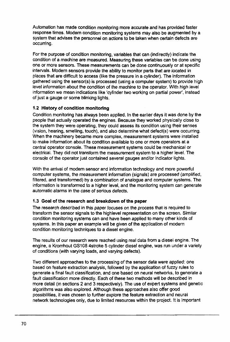
70

Automation has made condition monitoring more accurate and has provided faster response times. Modern condition monitoring systems may also be augmented by a system that advises the personnel on actions to be taken when certain defects are occurring.

For the purpose of condition monitoring, variables that can (indirectly) indicate the condition of a machine are measured. Measuring these variables can be done using one or more sensors. These measurements can be done continuously or at specific intervals. Modern sensors provide the ability to monitor parts that are located in places that are difficult to access (like the pressure in a cylinder). The information gathered using the sensor(s) is processed (using a computer system) to provide high level information about the condition of the machine to the operator. With high level information we mean indications like 'cylinder two working on partial power'. instead of just a gauge or some blinking lights.

1.2 History of condition monitoring Condition monitoring has always been applied. In the earlier days it was done by the people that actually operated the engines. Because they worked physically close to the system they were operating, they could assess its condition using their senses (vision, hearing, smelling, tOUCh), and also determine what defect{s) were occurring. When the machinery became more complex. measurement systems were installed to make information about its condition available to one or more operators at a central operator console. These measurement systems could be mechanical or electrical. They did not transform the measurement system to a higher level. The console of the operator just contained several gauges and/or indicator lights.

With the arrival of modern sensor and information technology and more powerful computer systems, the measurement information (signals) are processed (amplified, filtered, and transformed) by a combination of analogue and computer systems. The information is transformed to a higher level, and the monitoring system can generate automatic alarms in the case of serious defects.

1.3 Goal of the research and breakdown of the paper The research described in this paper focuses on the process that is required to transform the sensor signals to the highlevel representation on the screen. Similar condition monitoring systems can and have been applied to many other kinds of systems. In this paper an example will be given of the application of modern condition monitoring techniques to a diesel engine.

The results of our research were reached using real data from a diesel engine. The engine, a Kromhout GS1 08 4stroke 5 cylinder diesel engine, was run under a variety of conditions (with varying loads, and varying defects).

Two different approaches to the processing of the sensor data were applied: one based on feature extraction analysis, followed by the application of fuzzy rules to generate a final fault classification, and one based on neural networks, to generate a fault classification more directly. Each of these two methods will be described in more detail (in sections 2 and 3 respectively). The use of expert systems and genetic algorithms was also explored. Although these approaches also offer good possibilities, it was chosen to further explore the feature extraction and neural network technologies only, due to limited resources within the project. It is important

to note that the data upon which this research was based was real data, as measured on a diesel engine that is part of a dieselelectric generator set.

The implementation of the experimental prototype is discussed in section 4. A discussion and references are presented in sections 5 and 6.

The project involved TNOFEL and two other partners: • TNO Physics and Electronics Laboratory (TNOFEL), that has knowledge and

experience with modern information processing techniques . • TNO Centre for Mechanical Engineering (TNOMIT), that has expertise in the

modelling and simulation of mechanical systems, in condition monitoring systems and in measurement techniques.

• Royal Netherlands Naval Academy (RNINC), that provided a test facility consisting of the Kromhout diesel engine, and where the measurements were done. Knowledge about condition monitoring and modelling of diesel engines is available at the RNINC.

For a more detailed description of the techniques used in the project, see Meiler & Maas [1], and for the results see Meiler, Maas, Brockhoff, Tromp & Popma [2]. A literature study on artificial intelligence in condition monitoring systems is provided by Paas [3]. An extensive study on condition monitoring applied to diesel engines (using a model based technique) can be found in Bonnier [4], while specific knowledge about the engines is presented in Grohe [5].

2 Feature extraction and recognition technique

Feature extraction and recognition algorithms are used for analysing signals and for classifying signals into classes. In the simplest form, each class indicates a condition (e.g. OK / NotOK, or a more speCific condition like lowpowerforcylinder2). The classification is done by matching features of the signal, or the complete sensor signal, with a set of reference signals. The sensor signal will be classified as member of the class that correspond with the best matching reference signal.

In some cases, we don't need the complete signal to solve the classification problem. The isolation of those features of the signal that are unique for the classes results into a better and more efficient control of the classification problem. In that case, the influence of fluctuations in the sensor signal which are caused by instabilities, noise, and defects that have not been considered will be reduced to a minimum.

2.1 Necessary knowledge and information

While developing a condition monitoring system, the contribution of the process expert is directed towards informing the signal analyst about the (expected) behaviour of the sensor signals and little towards to physical process knowledge of the machine. This implies that this method is suitable to monitor machines for which an accurate enough model is not available.

The communication between the process expert and the signal analyst is essential because of the fact that the signal analyst must know which features of the sensor signal are strongly correlated to the malfunctions of the machine and how they relate to the control signals and operation/environs conditions. This is certainly true for complex sensor signals.

71

72

2.2 Important issues and problems In these cases, the condition monitoring system must be able to predict the signal behaviour for each defect over a wide range of operating/environs conditions and requires a mathematical description or at least a lookup table for each feature that corresponds with a defect. A lot of effort is needed to develop the feature extraction and classification algorithms, and depending on the complexity of the signals, high performance computing techniques and systems might be needed.

The isolation of features from the sensor signal has the benefit that several defects can be detected independently, using the same signal, if there is no correlation or overlap in the pattems of the features for the different defects.

2.3 Generalisation, adaptlveness and flexibility A feature recognition based condition monitoring system can be extended with new functionality for the detection of new defects without changing the settings of already existing functions. In fact, such a modular construction of the condition monitoring system has the benefit that already existing modules can be reused in the . implementation of new functions.

In general, experiences have indicated that a lot of effort is needed to get effective solution with this method. This is caused by the fact that a lot of effort is needed to analyse the defect with the corresponding sensor signal(s) and to determine the algorithms to isolate the features that are used for the classification.

Resuming, the advantages of a feature extraction and recognition based condition monitoring system are:

• Less process and model knowledge is needed compared to the first principle approach (a first principle model is a highly detailed physical mathematical model to predict the behaviour of machinery).

• The algorithms will only be triggered by predefined behaviour (features) of the sensor signals to reduce the influence of noise.

• The decision process is retraceable: The usage of well defined algorithms allows us to tell which classification corresponds with which sensor, and how this decision is made.

• This method is suitable for machines for which an accurate enough mathematical model is not available.

The disadvantages of this method are:

• Detailed knowledge of the behaviour of the sensor signal(s) is needed to determine which features of the signals are relevant and which features are not.

• A lot of effort is needed for developing the feature extraction and classification algorithms.

• Depending on the complexity of the signals, high performance computing techniques might be needed.

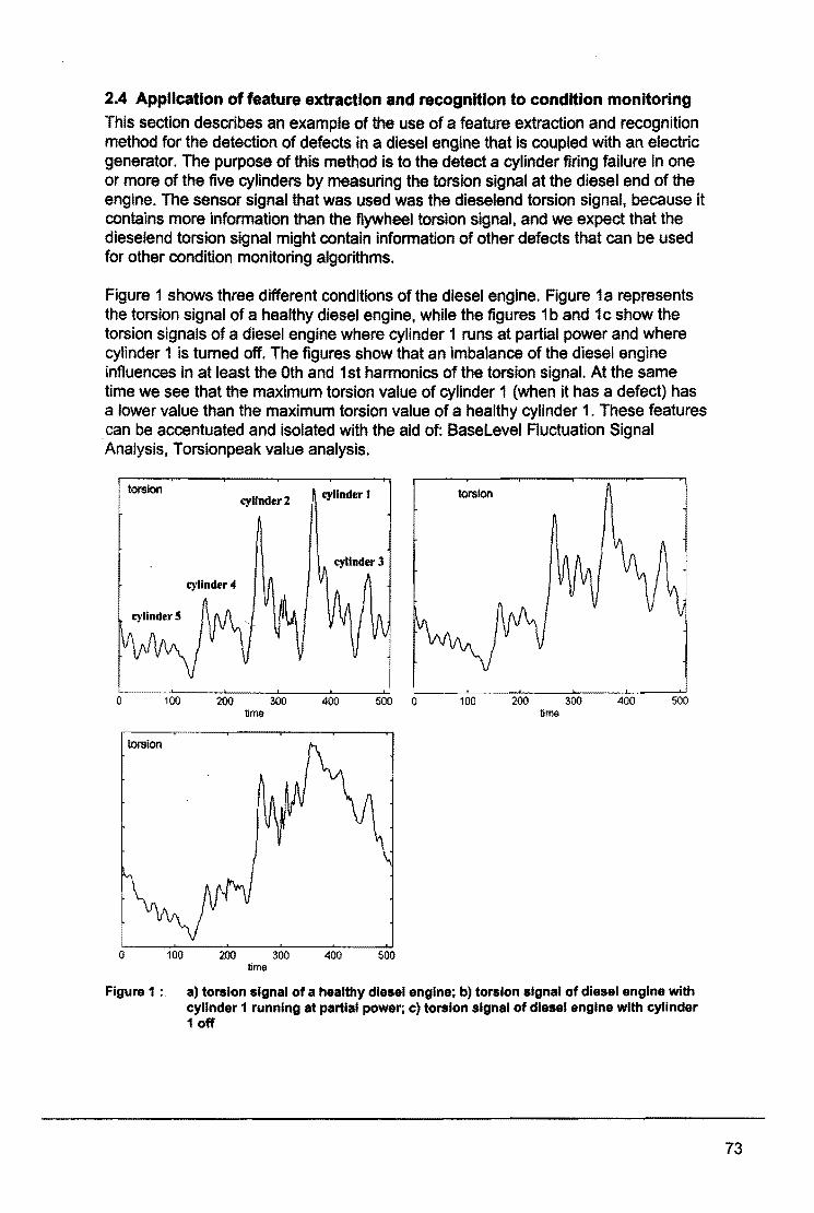
2.4 Application of feature extraction and recognition to condition monitoring This section describes an example of the use of a feature extraction and recognition method for the detection of defects in a diesel engine that is coupled with an electric generator. The purpose of this method is to the detect a cylinder firing failure in one or more of the five cylinders by measuring the torsion signal at the diesel end of the engine. The sensor signal that was used was the dieselend torsion signal, because it contains more information than the flywheel torsion signal, and we expect that the dieselend torsion signal might contain information of other defects that can be used for other condition monitoring algorithms.

Figure 1 shows three different conditions of the diesel engine. Figure 1a represents the torsion signal of a healthy diesel engine, while the figures 1 band 1 c show the torsion signals of a diesel engine where cylinder 1 runs at partial power and where cylinder 1 is turned off. The figures show that an imbalance of the diesel engine influences in at least the Oth and 1 st harmonics of the torsion signal. At the same time we see that the maximum torsion value of cylinder 1 (when it has a defect) has a lower value than the maximum torsion value of a healthy cylinder 1. These features can be accentuated and isolated with the aid of: Base Leve I Fluctuation Signal Analysis, Torsionpeak value analysis.

torsion cylinder 1 cylinder 1 torsion

cylinder 4

o 100 200 300 400 500 0 100 200 300 400 500 time lime

time

Figure 1 :. a) torsion signal of a healthy diesel engine; b) torsion signal of diesel engine with cylinder 1 running at partial power; c) torsion signal of diesel engine with cylinder 1 off

73

74

2.4.1 Baselevel fluctuation signal analysis The baselevel fluctuation signal is derived using five paints. These five paints represent the location of the start of the compression of each cylinder. A cubic interpolation algorithm is used to determine the ultimate baselevel signal function. The amplitude of the interpolated signal gives an indication about the kind of defect. The amplitude is very small in case of a healthy diesel engine. A large amplitude represents a cylinder off failure while a small amplitude represents a partial power failure. The point of time where the baselevel function reaches its maximum value indicates which cylinder doesn't work well (see figure 2).

Base-Level Fluctuation Signal (BlF) _ction

100 200 300 400 time

Figure 2: a) cylinder 1 running at partial power; b) cylinder 1 Is turned off

Base-Level FkJctuation Signal (BLf) _cUon

, '

500 time

The fact that the baselevel fluctuation signal is spread out over the complete combustion cycle gives us the ability to locate at most one defect in one of the five cylinders.

2.4.2 Torsion peak value analysis The torsion-peak analysis starts with taking the difference between the diesel end torsion signal and the baselevel fluctuation signal. In the resulting torsion signal we see that defects (like a cylinder off) are more visible than in the original signal. Figure 3 shows the examples of the corrected torsion Signals of two defects and a healthy diesel engine. Figure 3a (healthy engine) shows us that the torsion peak value of cylinder 1 is greater than the peak value of cylinder 2, the torsion peak value of cylinder 2 is greater than the peak value of cylinder 3, etc. In figure 3b we see that the peak value of cylinder 1 gets smaller if we introduce a small defect in cylinder 1 by running this cylinder at partial power. The peak value becomes even much smaller after turning off cylinder 1. In practice, we don't compare the peak values of each cylinder with each other, but we compare the peak value with a reference peak value for each cylinder. These reference values represent the mean peak values for a healthy diesel engine.

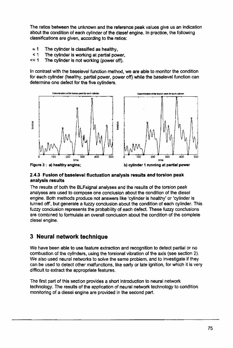
The ratios between the unknown and the reference peak values give us an indication about the condition of each cylinder of the diesel engine. In practice, the following classifications are given, according to the ratios:

::::: 1 The cylinder is classified as healthy, <1 The cylinder is working at partial power,

« 1 The cylinder is not working (power off),

In contrast with the baselevel function method, we are able to monitor the condition for each cylinder (healthy, partial power, power off) while the baselevel function can determine one defect for the five cylinders.

OeIe!mInatiOn ofllle torsion p •• kfor .ach <YIInder

time time

Flgure"3: a} healthy engine; b) cylinder 1 running at partial power

2.4.3 Fusion of baselevel fluctuation analysis results and torsion peak analysis results The results of both the BLFsignal analyses and the results of the torsion peak analyses are used to compose one conclusion about the condition of the diesel engine. Both methods produce not answers like 'cylinder is healthy' or 'cylinder is turned off', but generate a fuzzy conclusion about the condition of each cylinder. This fuzzy conclusion represents the probability of each defect. These fuzzy conclusions are combined to formulate an overall conclusion about the condition of the complete diesel engine.

3 Neural network technique

We have been able to use feature extraction and recognition to detect partial or no combustion of the cylinders, using the torsional vibration of the axis (see section 2). We also used neural networks to solve the same problem, and to investigate if they can be used to detect other malfunctions, like early or late ignition, for which it is very difficult to extract the appropriate features.

The first part of this section provides a short introduction to neural network technology. The results of the application of neural network technology to condition monitoring of a diesel engine are provided in the second part.

75

76

3.1 Introduction to neural networks

It is not always possible, or it can at least be very difficult and timeconsuming, to create and verify a classification method for purposes like the one that is discussed in this report (the condition monitoring problem) using conventional algorithms. This is especially true if we do not know enough about the characteristics of the data that we want to classify.

Because neural networks are trained, they adapt themselves to the characteristics of the training data. This allows a classifier, based on a neural network, to be trained without having detailed information about the characteristics of the data, instead of developed using a model or extensive knowledge of the process that provides the data that must be classified. This is especially useful when processing a complicated signal like the torsional vibration of a diesel engine.

Neural networks are parallel information processing systems. The structure and behaviour of a neural network is in some respects similar to a biological nervous system. A neural network consists of many, yet very simple, processing elements, called neurons. A neuron integrates the functionality of both memory and computation. The neurons of a neural network are, often very densely, connected to each other. A weight is associated with each connection between two neurons. As an example, the weight of a connection between neuron A and neuron B determines the influence that the output of a neuron A has on the input of neuron B.

3.1.1 Neural network architecture

Different neural network architectures use different connection patterns or topologies:

• All neurons are connected to each other (Hopfield network). The input pattern is supplied to each neuron and the output pattern is provided by each neuron.

• The network is organised in layers. A layer consists of several neurons. The output of each neuron in a layer is connected to the input of each neuron of the layer above. Neurons within the same layer are not connected to each other. The input pattern is supplied to the neurons in the lowest (input) layer. The output pattern is provided by the neurons of the highest (output) layer. There can be one or more hidden layers between the input and the output layers. These layers are called hidden because they are not accessible directly from outside the network (they are only connected to other layers in the network) .

• The topology of a network can also be specially optimised for a speCific purpose. These kind of networks require more knowledge about the problem to be solved and often lose there capability to be generally applicable.

A graphical representation of a twolayer neural network (the input layer is not an active layer because it only distributes the input values, and is not counted) is presented in figure 4.

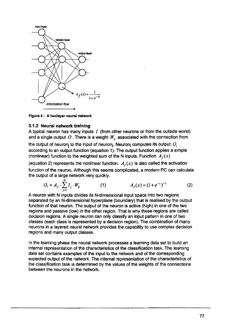
input layer

information flow

1 Aj(x}=--

t+e-x

Figure 4: A twolayer neural network

3.1.2 Neural network training A typical neuron has many inputs I (from other neurons or from the outside world) and a single output O. There is a weight Wy associated with the connection from

the output of neuronj to the input of neuronj. Neuroni computes its output OJ according to an output function (equation 1). The output function applies a simple (nonlinear) function to the weighted sum of the N inputs. Function A,(x)

(equation 2) represents the nonlinear function. A/x) is also called the activation

function of the neuron. Although this seems complicated, a modem PC can calculate the output of a large network very quickly.

N

q=A,·IIj.Wy (1) A,(x)=(1+e-X f) (2) j%1

A neuron with N inputs divides its N-dimensional input space into two regions separated by an N-dimensional hyperplane (boundary) that is realised by the output function of that neuron. The output of the neuron is active (high) in one of the two regions and passive (low) in the other region. That is why these regions are called decision regions. A single neuron can only classify an input pattern in one of two classes (each class is represented by a decision region). The combination of many neurons in a layered neural network provides the capability to use complex decision regions and many output classes.

In the learning phase the neural network processes a learning data set to build an internal representation of the characteristics of the classification task. The learning data set contains examples of the input to the network and of the corresponding expected output of the network. The internal representation of the characteristics of the classification task is determined by the values of the weights of the connections between the neurons in the network.

77

78

During the training process, the weights are altered according to a learning rule. There are many learning rules. As an example, a learning rule can determine the change in the weights based on the difference between the expected output of the network and the current output of the network. The data set must be presented to the network many times to let the weights converge to optimal values. Because of that, especially when large data sets are used, training can be slow.

The theory of neural network technology is not discussed further in this study. For more information about that topic, see Aleksander & Morton [6], Khanna, [7] and Lippmann [8].

3.1.3 Neural network advantages and disadvantages

In the summary below, the advantages and disadvantages for the application of neural network technology are presented:

Advantages: • No model is needed (Le. no inputoutput relationship has to be known) • Realtime performance is attainable

Disadvantages: • Training requires specific knowledge and experience with neural network

technology • No inSight into the classification process is gained • The reliability can only been assessed statistically, using a separate test data set • Very large data sets are needed, and training can be slow

3.2 Application of neural networks to condition monitoring

Neural network technology has been applied to condition monitoring of a diesel engine. The information to be used was the diesel end torsion signal. The engine was regarded as a 'black box'. The inputoutput relationship was unknown. The only thing that was available was a dataset consisting of many gigabytes of data. The dataset contains data of the healthy condition of the engine, and data when one or more defects were introduced or simulated. A neural network was to be used to classify a signal from the dataset as corresponding to a specific class (e.g. healthy, cylinder1defect, cylinder2partialpower, etc.).

Given these facts, the back propagation algorithm was used to train several twolayer neural networks. The algorithm was capable to adjust its learning rate autonomously, depending on the development of the network error. First a simple network was trained, that could only discern between the healthy and nothealthy state. Progressively more complicated networks were trained, capable to classify a growing combination of defects. For this purpose, the dataset was split in a training set and a test set. A network was trained for a number of training cycles, then tested against the test set. If the performance was sufficient, training was stopped. If the performance was not sufficient, training was continued. This process was continued until the performance became sufficient, or until the maximum number of training cycles was reached. If a network could not be trained successfully, the number of hidden units was increased. This process of network training was automated for a large part, with minimal human interaction.

35 neural networks were trained to classify the following defects: defects performance (in % ) defects performance (in %, )

h 10 100 h2li 155 2li 125 94 - -

h 10 20 100 h 2p 20 2li 155 2li 125 h 10 20 30 100 h 2lk 0.3

-h 10 20 30 40 100 h 2lk 0.3 20 -h 10 20 30 40 50 100 h 2lk 0.3 2lk 1.8 h 10 20 100 h 1p 100 h 10 20 2p+10 2p+30 100 h 2p 100 h 10 20 2p+10 2p+30 100 h 4p 100 h 1 75 h 5p 100 h 1 1+2p h 1p 2p laO h 1 1+2p 1+2p+50 h 1p 2p 4p 91 h e 100 h 1p 2p 4p 5p 93 h e e+2p h 2li 125 100

-h e e+2p e+2p+50 h 2lk 3.0 100

-h20 h27 h30 83 h 10 20 30 40 50 Ip 100 h I 83 h 10 20 30 40 50 1p 2p 100 h 2p 20 2p+10 2p+30 h 10 20 30 40 50 1p 2p 100

h 10 20 30 40 50 1p 2p 4p 5p 78

Legenda for table above: h = healthy, 0 = off, P = partial power, i = low injection pressure, I = late injection, e = early injection, Ik = leak in cylinder. A .. implies that a network could not be trained successfully.

Note that the training set was limited by the measurements that were available. This implied that not all combinations of defects could be trained. The measurement signals were preprocessed extensively using the following steps: resampling (to 'synchronise' the signal in neat bins of 512 samples per combustion cycle), filteril1g, averaging, peak removal, and normalising. Each value of a 512bin sample is mapped on one neuron of the input layer of the network. Each neuron in the output layer represents one class of defects. Postprocessing is done by only accepting a neural network classification if the neural network output values comply with the threshold values and if the 'distance' between the highest output neuron value and the nexthigher value exceeds a threshold. Also, in reality classification will only be accepted if it has occurred for a minimum number of times within a fixed time period.

4 Implementation

In the prototyping and experimentation phase of the project an experimental software prototype was implemented. The measurement data were preprocessed, made accessible, and organized. A demonstrator was built, based on the prototype.

The experimentation was mainly done in the Matlab [9] environment on IBM-PC compatible computers. Matlab is an environment that allows performing mathematical operations on large amounts of data interactively. It also incorporates an interpreted programming language. The Matlab Neural Network [10] toolbox was used extensively.

79

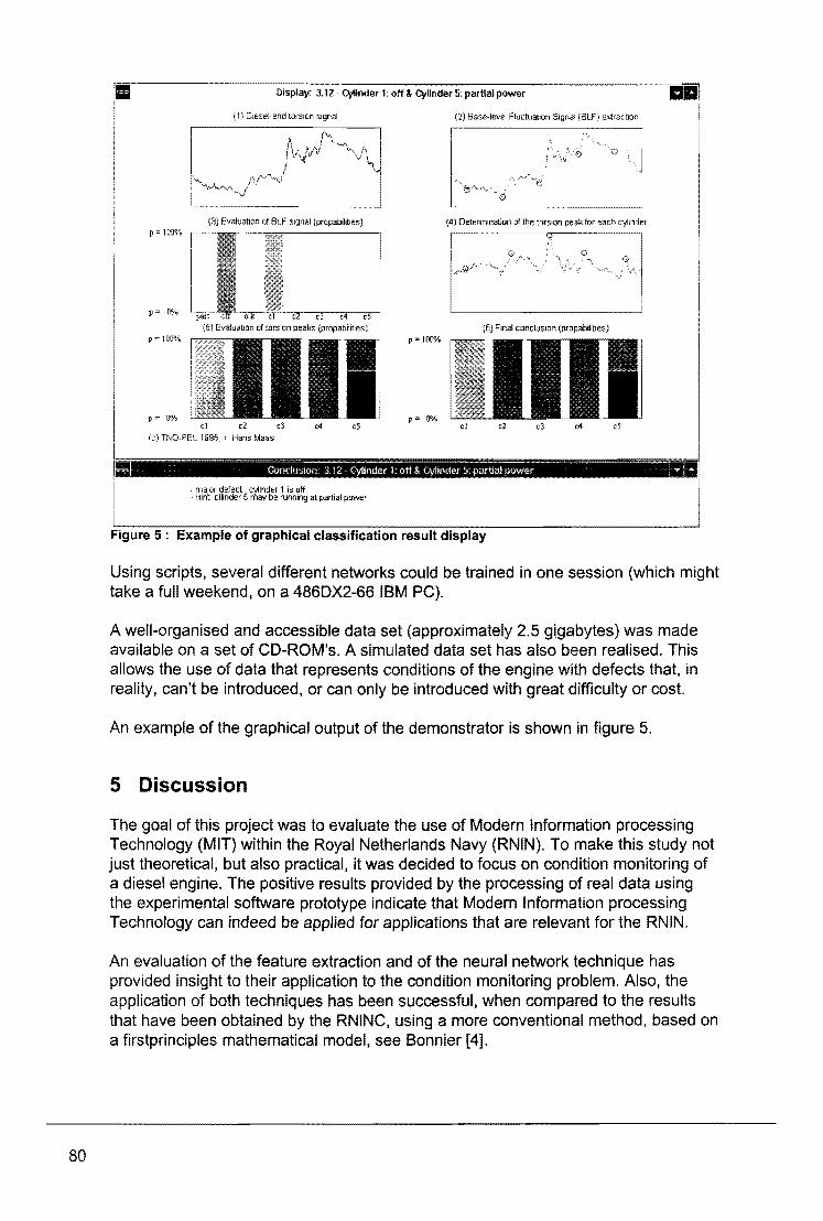
80

Display: 3.12 - CYlinder 1; off & CYlinder 5: partial power

(1) Diesel-end torsion signal (2) Base-level Flurn.atlon Signal [BLF) e:xtracbon

'0

(3) Evaluation of BLF signal (propabili!Jes) (4) Determination of the torSion peak for each cylinder p= lOOVt>

p= 0%

(6) Final conclUSion (propabiIiMs) P 100''10

p~ 0% c1 ,2 <3 c4 c5

p~ 0%

re) TNO-FEL 1995, Ir, Hans Maas

Figure 5: Example graphical classification result display

Using scripts, several different networks could be trained in one session (which might take a full weekend, on a 486DX2-66 IBM PC).

A well-organised and accessible data set (approximately 2.5 gigabytes) was made available on a set of CD-ROM's. A simulated data set has also been realised. This allows the use of data that represents conditions of the engine with defects that, in reality, can't be introduced, or can only be introduced with great difficulty or cost.

An example of the graphical output of the demonstrator is shown in figure 5.

5 Discussion

The goal of this project was to evaluate the use of Modern Information processing Technology (MIT) within the Royal Netherlands Navy (RNIN). To make this study not just theoretical, but also practical, it was decided to focus on condition monitoring of a diesel engine. The positive results provided by the processing of real data using the experimental software prototype indicate that Modern Information processing Technology can indeed be applied for applications that are relevant for the RNIN.

An evaluation of the feature extraction and of the neural network technique has provided insight to their application to the condition monitoring problem. Also, the application of both techniques has been successful, when compared to the results that have been obtained by the RNINC, using a more conventional method, based on a firstprinciples mathematical model, see Bonnier [4].

An operational version of this system can be applied to monitor the condition of dieselpowered electricity generators, and it is expected that it can also be applied to the main propulsion diesel engines and other equipment that incorporates internal combustion engines.

The results of the research into these two techniques are discussed below. For each of the two techniques, the discussion is split in two separate parts. The first part provides a general discussion about the approach (compared to other approaches), and the second part provides a discussion about the application of the approach as applied to condition monitoring within this project.

5.1 Feature extraction and recognition: general discussion In comparison with the first principles based method, none or less process knowledge of the machine is needed. This implies that this method is suitable for machines for which an accurate enough mathematical process model isn't available. However, this method requires knowledge about the signal behaviour versus machine defects, input signals and environs conditions.

While developing a condition monitoring system, the contribution of the process expert is directed towards informing the Signal analyst about the (expected) behaviour of the sensor Signals and little towards to physical process knowledge of the machine. The communication between the process expert and the signal analyst is essential because of the fact that the signal analyst must know which features of the sensor Signal are strongly correlated to the defects of the machine and to how these defects relate to the control signals and operation/environs conditions. This is certainly true for complex sensor signals.

In the case of complex signals, the condition monitoring system must be able to predict the signal behaviour for each defect over a wide range of operating/environs conditions and requires a mathematical description or at least a lookup table for each feature that corresponds with a defect. Our experiences have indicated that a lot of effort is needed to develop the feature extraction and classification algorithms, mainly because of the need to analyse the correlation between a defect and the corresponding features in the sensor signal(s). Depending on the complexity of the signals, high performance computing techniques and systems might be needed.

The isolation of features from the sensor signal has the benefit that several defects can be detected independently, using the same signal, if there is no correlation or overlap in the patterns of the features for the different defects.

A feature recognition based condition monitoring system can be extended with new functionality for the detection of new defects without changing the settings of already existing functions. In fact, such a modular construction of the condition monitoring system has the benefit that already existing modules can be reused in the implementation of new functions.

81

82

5.2 Feature extraction and recognition: case related discussion Two generic signal processing algorithms have been developed. Each of these methods is able to detect and locate two kinds of defects (cylinder off and cylinder running at partial power) in a diesel engine. The two methods are:

• Baselevel Fluctuation (BlF) signal analysis • Cylinder Torsionpeak signal analysis

The first method is used to detect and locate at most one defect in at most one cylinder. This defect will be called the major defect. The second method detects and locates at most one defect for each cylinder. The reliability of the BlFmethod is greater than the reliability of the cylinder Torsionpeak analysis method.

The Results of these two condition monitoring methods are combined to a single conclusion. On account of the difference of reliability of the two methods, the results of the BlFmethod overrule the results of the TorsionPeak analysis method for that particular cylinder containing the major defect. The remaining defects, as indicated by the cylinder TorsionPeak analysis are indicated as 'hints' because of the relatively lower reliability. The reliability of the TorsionPeak analysis is lower for those cylinders that are situated near the flywheel.

5.3 Neural networks: General discussion In comparison with the feature extraction and recognition method, even less process knowledge of the machine is needed. Because a neural network is not programmed, but trained, the fact that we do not know much about the characteristics of the data that we want to classify is often not (or less of) a problem when using neural networks. Gathering the learning data set (together with choosing a neural network paradigm) is the task that replaces the classical algorithm design process. The preprocessing step, that must transform the input into an input pattern which is suitable for processing by a neural network, can be a difficult task, especially when large data sets are involved.

The knowledge stored in the weights can't be extracted from the network, so that it will never be known which specific knowledge is used by the network.

Neural network technology will become more easy to use, as better toolkits (e.g. for Matlab) become available, and as faster computer systems with more memory (to store and process the training pattern data) become available.

It is never possible to prove the quality of a neural network based classifier deterministically. Using statistical techniques (based on a separate test data set), the performance of such a system can be determined.

Application of neural network technology requires a large data set, covering all classes of conditions that are required to be detected.

5.4 Neural networks: case related discussion The diesel end torsion signal was preprocessed and used as the input to the neural network. A data set consisting of many gigabytes of data was used. The data set contains data of the healthy condition of the engine, and data when one or more defects were introduced or simulated.

The backpropagation algorithm was used to train several twolayer neural networks, which were progressively more complicated. The networks were capable to indicate when a cylinder is not working, or when a cylinder is working on partial power. This performance is less for those cylinders that have less influence on the sensor signal. Other effects, like early I late ignition, can sometimes be recognised. This might be improved when more training data would be available.

It is expected that this technology can also be applied to similar systems, incorporating internal combustion engines.

6 References

[1] Meiler P.P., Maas H.L.M.M., Results of the technical analysis phase the MIT project, FEL94A354, TNOFEL, P.O. Box 96864, 2509 JG The Hague, The Netherlands.

[2] Meiler P.P., Maas H.L.M.M., Brockhoff H.S.T., Tromp C.A.J., Popma T., Final report ofthe project "Modem Information processing Technology (MIT}", FEL95A171, TNOFEL, P.O. Box 96864,2509 JG The Hague, The Netherlands.

[3] Paas M.H.J.W., Artificial Intelligence applications in condition monitoring, 95CMCR0621, TNOCMC, P.O. Box 49, 2600 AA Delft, The Netherlands.

[4] Bonnier J.S., Torsietrillingsanalyse t.b. v. de conditiebewaking van zuigerverbrandingsmotoren / Torsional vibration analysis for condition monitoring of internal combustion engines, parts 13, OEMO 94/08, Faculty of Maritime Technology, Delft University of Technology, The Netherlands, or ISSN 09236589, Royal Netherlands Naval Academy, P.O. Box 10.000,1780 CA Den Helder, The Netherlands.

[5] Grohe H., Benzine en diese/motoren: Werking, constructie en berekening van tweeslag en vierslagverbrandingsmotoren / Gas and diesel engines: Working, construction and design of two and fourstroke internal combustion engines, Kluwer Technische Boeken B.V., Deventer, The Netherlands.

[6] Aleksander I., Morton H., An introduction to Neural Computing, Chapmann & Hall, ISBN 0412377802,1990

[7J Khanna T., Foundations of Neural Networks, AddisonWesley Publishing Company, ISBN 0201500361, 1990

[8] Lippmann R.P., An Introduction to Computing with Neural Nets, IEEE ASSP Magazine, pp. 422, April 1987

[9] Mathworks, Matlab User's Guide, The Mathworks, Inc., 24 Prime Park Way, Natick, Mass. 01760, USA.

[10] Mathworks, Neural Network User's Guide, The Mathworks, Inc., 24 Prime Park Way, Natick. Mass. 01760. USA.

83

Middagsessie 2

oJ.v. prof.dr.ir W.M.G. van Bokhoven

85

86

Biografie

Ton de Weijer is in 199~afgestt;J(!Ie$rd aan de Katholieke Universiteit Nijmegen. In datzeLf."jaar kwamNjindienst als Junior Onderzoeker op de afdeling Analytiscfije'Ghemie van de KUNVoor het verrichten van promotieonderzoek. Dit onde~oek is uitgevoe:ttdl in nauwe samenwerking met Akzo Nobel Cer:ltral Reseac~.1napril 1995 i&~tiin vaste diet'lstgetreden ~~fl1 laatst genoemde ondernemrlThtg •. Gi)rft!i~oeKsf:}e~: proces-s~tuur­eigenschappen relaties tb;v. flberbusiness units vamAkzo Nobel.

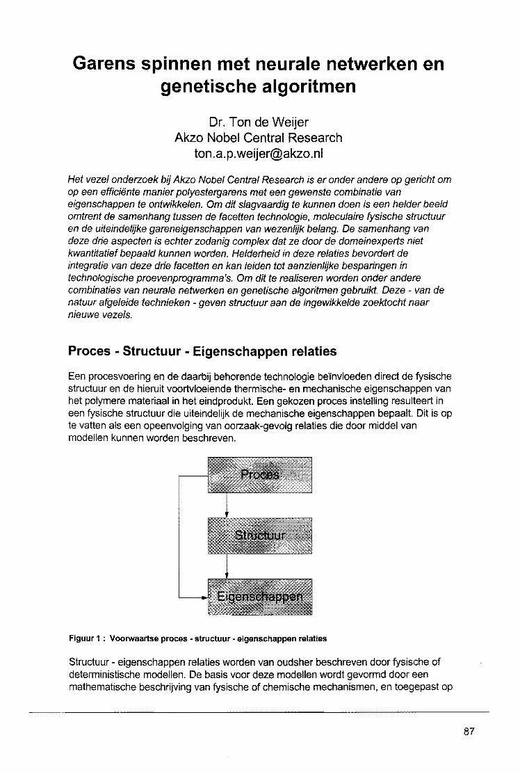
Garens spinnen met neurale netwerken en genetische algoritmen

Dr. Ton de Weijer Akzo Nobel Central Research

ton.a.p.weijer@akzo.nl

Het vezel onderzoek bij Akzo Nobel Central Research is er onder andere op gericht om op een efficiente manier polyestergarens met een gewenste combinatle van eigenschappen te ontwikkelen. Om dit slagvaardig te kunnen doen is een helder bee/d omtrent de samenhang tussen de facetten technologie, mo/eculaire fysische structuur en de uiteindelijke gareneigenschappen van wezenlijk belang. De samenhang van deze drie aspecten is echter zodanig complex dat ze door de domeinexperts niet kwantitatief bepaald kunnen worden. Helderheid in deze relalies bevordert de integratie van deze drie facetten en kan lelden tot aanzienlijke besparingen in technologische proevenprogramma's, Om dit fe realiseren worden onder andere comb/naties van neurale netwerken en genetische algoritmen gebruikt. Deze - van de natuur afgeleide technieken - geven structuur aan de ingewikkelde zoektochf naar nieuwe vezels.

Proces - Structuur - Eigenschappen relaties

Een procesvoering en de daarbij behorende technologie be'invloeden direct de fysische structuur en de hieruit voortvloeiende thermische- en mechanische eigenschappen van het polymere materiaal in het eindprodukt. Een gekozen proces instelling resulteert in een fysische structuur die uiteindelijk de mechanische eigenschappen bepaalt. Dit is op te vatten als een opeenvolging van oorzaak-gevolg relaties die door middel van modellen kunnen worden beschreven.

Figuur 1 : Voorwaartse proces • structuur • eigenschappen relaties

Structuur - eigenschappen relaties worden van oudsher beschreven door fysische of deterministische modellen. De basis voor deze modellen wordt gevormd door een mathematische beschrijving van fysische of chemische mechanismen, en toegepast op

87

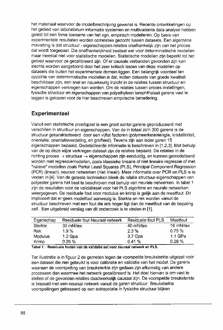
88

het materiaal waarvoor de modelbeschrijving gewenst is. Recente ontwikkelingen op het gebied van laboratorium informatie systemen en multivariante data analyse hebben geleid tot een forse toename van het zgn. empirisch modelleren. Op basis van experimentele resultaten worden correlaties gezocht tussen datasets. Een algemene misvatting is dat structuur - eigenschappen relaties onafhankelijk zijn van het proces dat wordt toegepast. Die onafhankelijkheid bestaat wei voor deterministische modellen maar meestal niet voor statistische modellen. Statistische modellen zijn beperkt tot het gebied waarvoor ze gecalibreerd zijn. Of er causale verbanden gevonden zijn kan slechts worden aangetoond door het zeer kritisch testen van deze modellen op datasets die buiten het experimentele domein liggen. Een belangrijk voordeel ten opzichte van deterministische modellen is dat, indien datasets van goede kwaliteit beschikbaar zijn, een snel en nauwkeurig inzicht in de relaties tussen structuur en eigenschappen verkregen kan worden. Om de relaties tussen proces instellingen, fysische structuur en eigenschappen van polyethyleen terephthalaat garens vast te leggen is gekozen voor de hier beschreven empirische benadering.

Experi menteel

Vanuit een statistische proefopzet is een groot aantal garens geproduceerd met verschillen in structuur en eigenschappen. Van de in totaal zo'n 300 garens is de structuur gekarakteriseerd door een vijftal factoren (polymeerketenlengte, kristalliniteit, orientatie, orientatieverdeling, en grofheid). Tevens zijn aan ieder garen 15 eigenschappen bepaald. Gedetailleerde informatie is beschreven in [1,2,3]. Met behulp van de op deze wijze verkregen dataset zijn de relaties bepaald. De relaties in de richting proces ~ structuur ~ eigenschappen zijn eenduidig, en kunnen gemodelleerd worden met regressiemodellen, zoals klassieke lineaire of niet lineaire regressie of met "na'ieve" modellen zoals Partial Least Squares (PLS), Principal Component Regression (PCR) (Iineair), neurale netwerken (niet lineair). Meer informatie over PCR en PLS is te vinden in [4]. Van de geteste technieken bleek de relatie structuur-eigenschappen van polyester garens het best te beschrijven met behulp van neurale netwerken. In tabel 1 zijn de resultaten voor de validatieset voor het PLS algoritme en neurale netwerken weergegeven. De residuele fout voor modulus en krimp is gelijk aan de meetfout. Dit impliceert dat er geen modelfout aanwezig is. Sterkte en rek worden vanuit de structuur beschreven met een fout die iets hoger ligt dan de meetfout van de bepaling zelf. Een uitgebreid verslag van dit onderzoek is te vinden in [1].

__ ~ig.~~_~~~§l.E .. _._ ..... _!3.~~9~~LE!l_!.~~! .. ~.~~~§l~~ne~er~_ .... _ .. __ .~~~!9~el~.!~_~! .. ~~~ ......... _~~.~!!~.~t Sterkte 30 mN/tex 40 mN/tex 16 mN/tex Rek 1.9 % 2.3 % 0.75 % Modulus 1.2 Gpa 3.7 Gpa 1.1 GPa Krimp 0.25 % 0.41 % 0.28 %

Tabel 1 : Residuele fouten van de validatie set voor neuraal netwerk en PLS.

Ter illustratie is in figuur 2 de gemeten tegen de voorspelde breuksterkte uitgezet voor een dataset die niet gebruikt is voor calibratie en validatie van het model. De garens waaraan de voorspelling van breuksterkte zijn gedaan zijn afkomstig van andere processen dan waarmee het netwerk gecalibreerd is. Het doel hiervan is om vast te stellen of de gevonden relaties daadwerkelijk causaal zijn. De voorspelde breuksterkte is bepaald met een neuraal netwerk vanuit de garen structuur. Breuksterkte voorspellingen gebaseerd op een extrapolatie in fysische structuur blijken

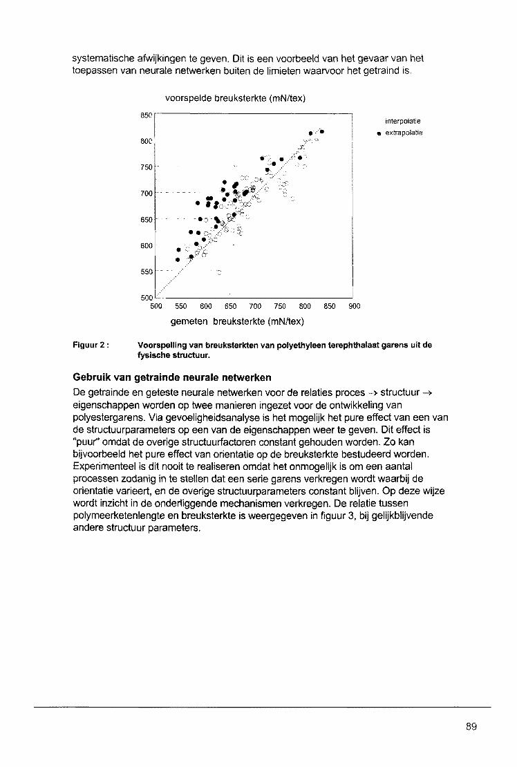
systematische afwijkingen te geven. Dit is een voorbeeld van het gevaar van het toepassen van neurale netwerken buiten de limieten waarvoor het getraind is.

Figuur2 :

voorspelde breuksterkte (mN/tex)

850,-------------------------------~

interpolatie

• extrapolatie 800

750 ...

700

650 ..

600

550

500~------------------------------~

500 550 600 650 700 750 800 850 900

gemeten breuksterkte (mN/tex)

Voorspelling van breuksterkten van polyethyleen terephthalaat garens uit de fysische structuur.

Gebruik van getrainde neurale netwerken

De getrainde en geteste neurale netwerken voor de relaties proces -+ structuur -+ eigenschappen worden op twee manieren ingezet voor de ontwikkeling van polyestergarens. Via gevoeligheidsanalyse is het mogelijk het pure effect van een van de structuurparameters op een van de eigenschappen weer te geven. Dit effect is "puur" omdat de overige structuurfactoren constant gehouden worden. Zo kan bijvoorbeeld het pure effect van orientatie op de breuksterkte bestudeerd worden. Experimenteel is dit nooit te realiseren omdat het onmogelijk is om een aantal processen zodanig in te stell en dat een serie garens verkregen wordt waarbij de orientatie varieert, en de overige structuurparameters constant blijven. Op deze wijze wordt inzicht in de onderliggende mechanismen verkregen. De relatie tussen polymeerketenlengte en breuksterkte is weergegeven in figuur 3, bij gelijkblijvende andere structuur parameters.

89

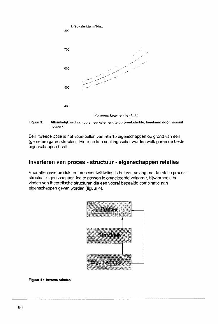
90

Figuur 3:

Breuksterkte mN/tex 800

700

600

500

400

Polymeer ketenlengte (A.U.)

Afhankelijkheid van polymeerketenlengte op breuksterkte, berekend door neuraal netwerk.

Een tweede optie is het voorspellen van aile 15 eigenschappen op grand van een (gemeten) garen structuur. Hiermee kan snel ingeschat worden welk garen de beste eigenschappen heeft.

Inverteren van proces - structuur - eigenschappen relaties

V~~r effectieve pradukt en pracesontwikkeling is het van belang om de relatie praces­structuur-eigenschappen toe te passen in omgekeerde volgorde. bijvoorbeeld het vinden van theoretische structuren die een vooraf bepaalde combinatie aan eigenschappen geven worden (figuur 4).

Figuur 4: Inverse relaties

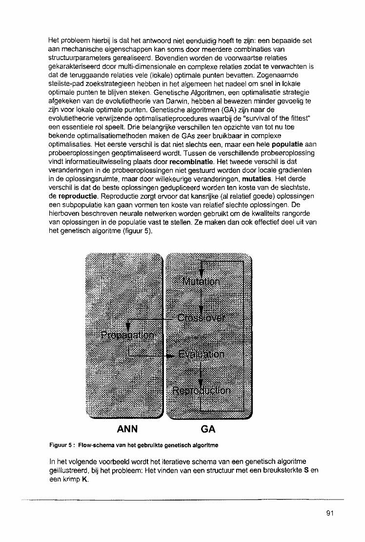
Het probleem hierbij is dat het antwoord niet eenduidig hoeft te zijn: een bepaalde set aan mechanische eigenschappen kan soms door meerdere combinaties van structuurparameters gerealiseerd. Bovendien worden de voorwaartse relaties gekarakteriseerd door multi-dimensionale en complexe relaties zodat te verwachten is dat de teruggaande relaties vele (lokale) optimale punten bevatten. Zogenaamde steilste-pad zoekstrategieen hebben in het algemeen het nadeel om snel in lokale optimale punten te blijven steken. Genetische Algoritmen, een optimalisatie strategie afgekeken van de evolutietheorie van Darwin, hebben al bewezen minder gevoelig te zijn voor lokale optimale punten. Genetische algoritmen (GA) zijn naar de evolutietheorie verwijzende optimalisatieprocedures waarbij de "survival of the fittest" een essentiele rol speelt. Drie belangrijke verschillen ten opzichte van tot nu toe bekende optimalisatiemethoden maken de GAs zeer bruikbaar in complexe optimalisaties. Het eerste verschil is dat niet slechts een, maar een hele populatie aan probeeroplossingen geoptimaliseerd wordt. Tussen de verschillende probeeroplossing vindt informatieuitwisseling plaats door recombinatie. Het tweede verschil is dat veranderingen in de probeeroplossingen niet gestuurd worden door locale gradienten in de oplossingsruimte, maar door willekeurige veranderingen, mutaties. Het derde verschil is dat de beste oplossingen gedupliceerd worden ten koste van de slechtste, de reproductie. Reproductie zorgt ervoor dat kansrijke (al relatief goede) oplossingen een subpopulatie kan gaan vormen ten koste van relatief slechte oplossingen. De hierboven beschreven neurale netwerken worden gebruikt om de kwaliteits rangorde van oplossingen in de populatie vast te stellen. Ze maken dan ook effectief deel uit van het genetisch algoritme (figuur 5).

ANN GA Figuur 5: Flow-schema van het gebruikte genetisch algoritme

In het volgende voorbeeld wordt het iteratieve schema van een genetisch algoritme ge'lIIustreerd, bij het probleem: Het vinden van een structuur met een breuksterkte S en een krimp K.

91

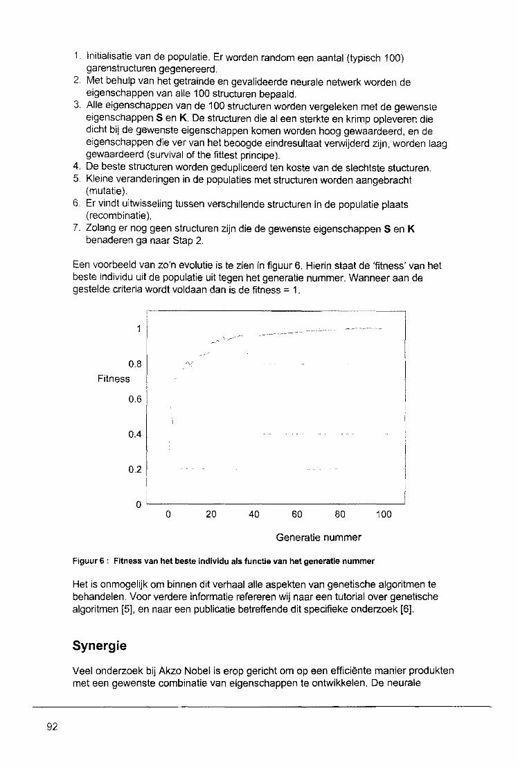
92

1. Initialisatie van de populatie. Er worden random een aantal (typisch 100) garenstructuren gegenereerd.

2. Met behulp van het getrainde en gevalideerde neurale netwerk worden de eigenschappen van aile 100 structuren bepaald.

3. Aile eigenschappen van de 100 structuren worden vergeleken met de gewenste eigenschappen Sen K. De structuren die al een sterkte en krimp opleveren die dicht bij de gewenste eigenschappen komen worden haag gewaardeerd, en de eigenschappen die ver van het beoogde eindresultaat verwijderd zijn, worden laag gewaardeerd (survival of the fittest principe).

4. De beste structuren worden gedupliceerd ten koste van de slechtste stucturen. 5. Kleine veranderingen in de populaties met structuren worden aangebracht

(mutatie). 6. Er vindt uitwisseling tussen verschillende structuren in de populatie plaats

(recombinatie) . 7. Zolang er nog geen structuren zijn die de gewenste eigenschappen S en K

benaderen ga naar Stap 2.

Een voorbeeld van zo'n evolutie is te zien in 'nguur 6. Hierin staat de 'fitness' van het beste individu uit de populatie uit tegen het generatie nummer. Wanneer aan de gestelde criteria wordt voldaan dan is de fitness = 1.

0.8

Fitness

0.6

0.4 -

0.2 1

o ~. --------------------------------------~ o 20 40 60 80 100

Generatie nummer

Figuur 6: Fitness van het beste individu als functie van hat ganeratie nummar

Het is onmogelijk am binnen dit verhaal aile aspekten van genetische algoritmen te behandelen. Voor verdere informatie refereren wij naar een tutorial over genetische algoritmen [5], en naar een publicatie betreffende dit specifieke onderzoek [6].

Synergie

Veel onderzoek bij Akzo Nobel is erop gericht om op een efficiente manier produkten met een gewenste combinatie van eigenschappen te ontwikkelen. De neurale

netwerken die hier gecombineerd zijn met genetische algoritmen kunnen direkte aanwijzingen geven in de richting waarin een structuur van een materiaal of een proces moet worden gestuurd om aan de gestelde specificaties te voldoen. Hier geldt dat er in de statistiek methoden voorhanden zijn die eenzelfde taak kunnen volbrengen. Of het gebruik van deze - van de natuur afgeleide - technieken een meerwaarde hebben, hangt af van factoren als volledigheid van de data, complexiteit van de relaties en het aantal beschikbare trainingsvoorbeelden. In het algemeen geldt dat neurale netwerken goed inzetbaar zijn in complexe relaties (niet monotoon stijgend of dalend, veer interacties tussen variabelen, enzovoort). Genetische algoritmen zijn vanwege het impliciet parallellisme, geschikt v~~r optimalisatietaken in complexe zoekruimten. In deze toepassing zijn genetische algoritmen en neurale netwerken dan ook een mooi voorbeeld van synergie.

Kennissysteem

De relaties tussen proces instellingen, fysische structuur en eigenschappen van polyethyleen terephthalaat zijn vastgelegd in een groot aantal neurale netwerken en genetische algoritmen. Samen met achtergrondkennis in de vorm van teksten en figuren zijn de relaties opgenomen in een gebruiksvriendelijk computersysteem genoemd BESSY. Op deze manier wordt de beschikbare kennis op een efficiente manier aangeboden aan de dome in experts. Medewerkers die onderzoek doen op het gebied van polyester vezels raadplegen dit systeem regelmatig. Zijn ervaren het systeem als een gebruiksvriendelijk, inspirerend en krachtig hulpmiddel bij de planning van nieuwe experimenten, procesontwikkeling en scholing.

Referenties

1. A.P. de Weijer, Process - Structure - Property Relationships obtained with Natural Computation, Thesis, Kath. Univ. Nijmegen 1995.

2. A.P.de Weijer and H.M. Heuvel, Neural Network Relations obtained from a Large Set of Data on Drawn Poly(ethylene Terephthalate) in Handbook of applied polymer processing, Marcel Dekker, New York, 1996 p385-409

3. A.P. de Weijer, L. Buydens, G. Kateman, H.M. Heuvel, Neural Networks used as a soft-modelling technique for quantitative description of the relation between physical structure and mechanical properties of poly(ethylene terephthalate) yarns, Chemom. Intell. Lab. Syst., 16 (1992) P 77-86

4. H. Martens and T. Naes, Multivariate Calibration, Wiley & Sons Ltd, ISBN 0-71-90979-3

5. C.B. Lucasius, G.Kateman, Understanding and using genetic algorithms. Part I.Concepts, properties and context, Chemometrics and intelligent laboratory systems, 19 (1993) 1-33 (tutorial)

6. A.P. de Weijer, C.B. Lucasius, L. Buydens, G. Kateman, H.M. Heuvel, H.Mannee, Using Genetic Algorithms for an Artificial Neural Network Inversion, Chemom. Intell. Lab. Syst., 20 (1993) p 45-55

93

94

Biografie

11\11. Helmut Brockmeyer (1M1) is sinCis~,~jn stuaie werkttflgbouw~uf)de aa~;ae KfS Amhem werkzaam bij Smit TransfQ~~,te;Wfj~n. Hij is ill dit be€lrijf in ver$<miJIende"fi:Jneti~sw __ a.i~weestMee$taI waren dezemmctleslnde vorm Van rt:lformatieverwerking tU$Sende Q~rpfase,en de r:woductie, met nam~ veFliieuwinril;}~iTn beEltijf$~

besturingssyS:temen, zeals autGmatisering vansmklijsten, werk-voorbereiding en planAinpn. De:;;la~tejal'enh~"~de heer BI'~mever vooral be~ metsystematlsch onderzoek iI:)¥p~tijden bijEfe enkelstuksproductmvan transformatoren om aedooJltbO,tijden te verkorten.

HiernaaSl:heeft Helm't;Jt Brockmeyer zich bezlggenoudenmetchet ontwikkelen en in bedr4jfsteHefl'V'an enkeJe geautomatiseerde cenenen nietlWe productiete(¥hnleken.

Neurale Netwerken bij Smit Transformatoren

H. Brockmeyer, Smit Transformatoren Tel 024-3568649

Smit Transformatoren, u vermoedde het ai, maakt transformatoren. Het bedrijf is opgericht in 1913 door Willem Smit. Het maken van transformatoren is geen lopende-bandwerk. Smit maakt transformatoren van 50 tot 1.000.000 kVA en een maximale bedrijfsspanning van 550.000 Volt.

Per jaar worden ongeveer 80 stuks afgeleverd, met een gemiddelde waarde van fl 2.000.000. Aile transformatoren lijken van buiten hetzelfde. De transformatoren worden echter op bestelling volgens klantspecificaties gemaakt. Dit betekent dat . twee transformatoren zelden precies hetzelfde zijn; iedere keer zjjn de specifieke wensen anders.

Er kan geen standaardproduct ontwikkeld worden die aan de meeste wensen van de klanten voldoel. De materiaalprijzen (die meer dan 50 procent van de kosten omvatten) zouden dan te hoog worden. Daarnaast is de factor arbeid verantwoordelijk voor 30 procent van de kostprijs. De materiaalprijs is vast; de arbeidskosten niet. De totale kosten kunnen geminimaliseerd worden door de werknemers optimaal in te zetten en de grondstoffen op tijd aan te voeren. Een goed planningsproces biedt een strategisch voordeel op de sterk concurrerende markt.

Het is moeilijk de planning te voorspeUen van een product, aangezien de verschillen erg groot zijn. Vroeger werd de planning geschat aan de hand van ervaringen van eerdere opdrachten. Zo'n vijftien jaar geleden was dit niet meer te rijmen met een modeme, efficiente bedrijfsvoering. Smit is toen begonnen met een uitgebreide analyse van de werkzaamheden en van de factoren die invloed hebben op de tijd die nodig is om een transformator te bouwen. Met het resultaat van deze studie zijn vervolgens formules ontwikkeld die gebruikt werden om voor iedere transformator te bepalen hoeveel tijd de verschillende productiestappen zouden vergen. Deze formules bevatten ongeveer 250 parameters en waren empirisch verkregen. Ze waren niet optimaal, doordat niet aUe parameters gemodelleerd konden worden. Door kleine veranderingen in het productieproces moesten de formules mee veranderen. Hiertoe werden eens per jaar de resultaten van de berekeningen met de werkelijk gebruikte tijd vergeleken. Op basis van de verschillen werden de formules handmatig aangepast.

In de loop van de tijd werden de formules steeds beter, maar echt bevredigend waren ze nooil. Experimenten met meervoudige lineaire regressies gaven ook niet de gewenste resultaten. Oit wordt onder andere veroorzaakt door gebrek aan voldoende gegevens. Tevens is de factor 'mens' in dit proces niet goed in te schatten.

95

96

Via het Innovatiecentrum Midden- en Zuid-Gelderland in Amhem is Smit in contact gekomen met Biologica, een bedrijf dat zich heeft gespecialiseerd in industri&le toepassingen van kunstmatige neurale netwerken. Bij het gebruik van neurale netwerken wordt niet gekeken naar de wetenschappelijke achtergrond; het wordt aileen maar gebruikt.

In eerste instantie werd het idee sceptisch ontvangen. Het was natuurlijk een geheel nieuwe techniek en slechts weinig mensen hadden er al ervaring mee opgedaan. Bij deze techniek was het niet nodig om zelf de factoren van de formules te bepalen. Het neurale netwerk 'Ieerde' zelf hoe bepaalde specificaties invloed hadden op de uitkomst. Het werd dus overbodig om handmatig aan de (ad hoc) formules te sleutelen. Door het neurale netwerk te trainen (gegevens met bijbehorende gerealiseerde tijden aan te bieden), kan het netwerk bij andere situaties zelfstandig een voorspelling doen.

Samen met Biologica is een onderzoek opgezet dat met weinig inspanning verrassend goede resultaten opleverde. De structuren met parameters en gegevens waren reeds beschikbaar en konden zo gebruikt worden om neurale netwerken te trainen. In een fractie van de tijd die nodig was om de formules te ontwikkelen (en actueel te houden), was het neurale netwerk in staat betere voorspellingen te maken. Op het ogenblik wordt de techniek geheel zelfstandig gebruikt. Om gemakkelijk gebruik te kunnen maken van het neurale netwerk, is het ge'fntegreerd in het bestaande spreadsheetprogramma, waarin de formules staan. De twee uitkomsten kunnen dan met elkaar vergeleken worden en als discussiestuk dienen voor de te plannen uren.

In figuur 1 staat een resultaat van de oude methode en van de neurale netwerken. Hieruit blijkt duidelijk dat de neurale netwerken een beter resultaat geven. Slechts in enkele gevallen was het verschil teleurstellend groot. Meestal ging het hierbij om transformatoren met een sterk afwijkende specificaties. Hiermee komt een tekortkoming van de techniek aan het licht: bij een sterk afwijkende input buiten het gebied van het geleerde is de output onbetrouwbaar. Binnen bepaalde tolerantie is een goede output gewaarborgd.

De netten moeten regelmatig bijgehouden worden. Ais de nieuwe situaties aan het net aangeboden worden, zal het netwerk deze kennis toepassen. Er moet echter gewaakt worden dat het netwerk niet 'overleerd' raakt. Dan zou de kwaliteit van de voorspellende resultaten afnemen. Veranderingen in het productieproces worden door het regelmatig leren (ongeveer een keer per jaar) door het neurale netwerk automatisch verwerkt.

De grilligheid van de mens kan natuurlijk niet in een geautomatiseerd proces gevangen worden; het net is bijvoorbeeld niet in staat iets als een griepepidemie te voorspellen.

Van het neurale netwerk mogen geen wonderen verwacht worden. Wei is het een heel handig hulpmiddei. Vooral nu prijzen en levertijden sterk onder druk staan, is het van groot belang doorlooptijden nauwkeurig te bepalen. Deze techniek biedt hierbij een uitkomst.

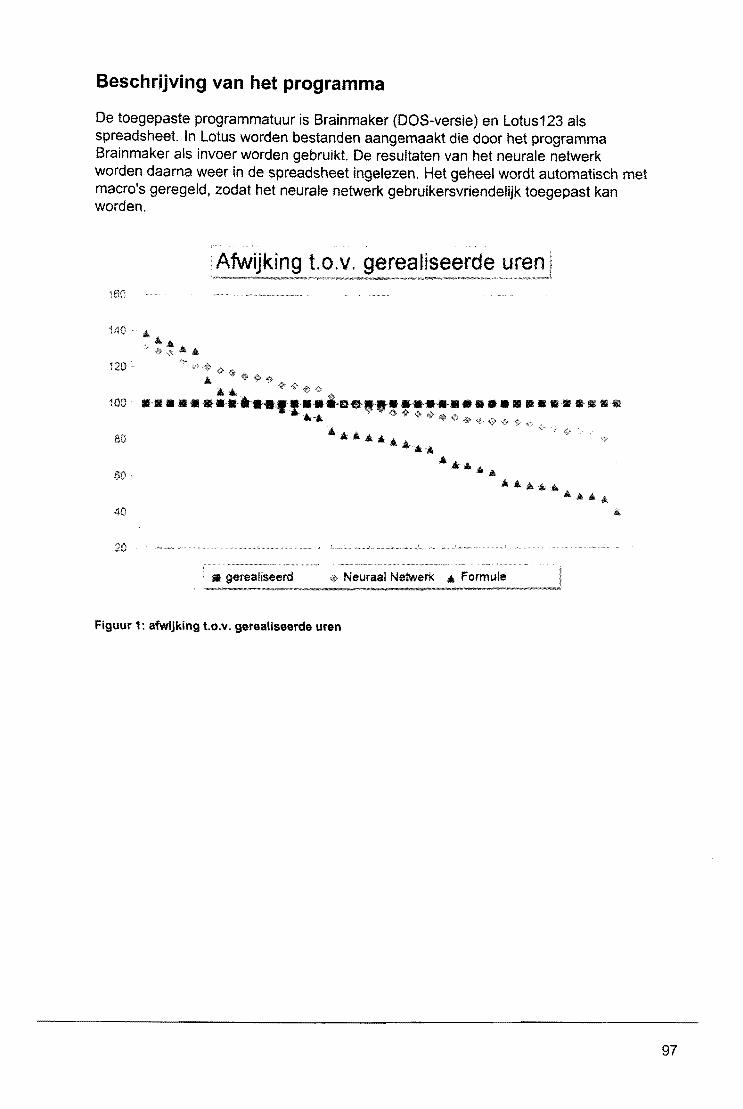
Beschrijving van het programma

De toegepaste programmatuur is Brainmaker (DOS-versie) en Lotus 123 als spreadsheet. In Lotus worden bestanden aangemaakt die door het programma Brainmaker als invoer worden gebruikt. De resultaten van het neurale netwerk worden daarna weer in de spreadsheet ingelezen. Het geheel wordt automatisch met macro's geregeld. zodat het neurale netwerk gebruikersvriendeiijk toegepast kan worden.

AfwiJking t.O.V. gereafiseerde uren I ''-'''' "''''_'''*. ~w"'~»~~"'-..,"''''''' _---w-,_,,~->'~ff'_~k~_'.''''.,.'''>:, •. ''''' •. w+'''/.»<»'''''0~

160

II gerealiseerd ~ Neuraal Netwerk ... Formule

Figuur 1: afwijking t.O.V. gerealiseerde uren

97

98

Biografie

RemcoFrenKen is in 1993 afgestudeerd in e.lektriciteitsYoorzienien hoogspanningstechniek aan (f~ liLJOelft. Sinds;;di d'werkt bij bijK:1!MA if7ll,Arnhem. fliJ>isLm~t;flame ~FKzaam in . .projecten ~l' hetwebied van mooerne con:JPtfterte'Clilnieken (fuzzy logic, neurate netwerken, genet$che algol'itmen1. Naast 06 projecten

"voorspelling waFmtevraa~!'eFl 'TUNOl'Iris rlij recentelijk betrokken g6weest bij de ontwikkeling van een fl...lZZY1ogic aefviessysteem voor de Kohonel'l classificatie opfletveiligheiden de1f'lodellering van vervuiting in inlaatfilters.

Neurale Netwerken in de energiesector; twee praktijkvoorbeelden

Remco Frenken, KEMA

Postbus 9035 6800 ET Arnhem

R.M.L.FRENKEN@MTA4.KEMA.NL

De afgelopen jaren heeft KEMA in een aantal situaties neurale netwerken toegepast. In deze voordraeht worden twee van deze toepassingen.besproken; de ontwikkeling van het adviessysteem TUNON voor de bedrijfsvoering van een elektrieiteitseentrale en de voorspelling van de warmte afname bij stadsverwarming. Aangegeven wordt waarom in genoemde situaties neurale netwerken zijn toegepast en wat de alternatieven zijn. Verder wordt gesproken over de problemen waar men in de praktijk mee fe maken krijgf, zoa/s se/eetie van de juiste parameters, verkrijgen van benodigde leer en testgegevens en het omgaan met "missing values" of onbetrouwbare gegevens. Een ander aspect is de befrouwbaarheid; hoe zeker is het dat het neurale netwerk het juiste antwoord geeft?

Inleiding

Sinds 1991 wordt bij KEMA onderzoek gedaan naar toepassingsmogelijkheden van neurale netwerken. De eerste jaren was dit onderzoek vooral exploratief van aard. Typiseh vragen uit die tijd zijn: wat zijn achterliggende ideaen bij NN, welke soorten bestaan er, hoe kun je ze gebruiken en wanneer gaan ze stuk. Een promotieonderzoek [1] leidde tot een blauwdruk voor concrete toepassingen in de elektriciteitssector; neurale netwerken bleken te kunnen worden toegepast bij het adaptief instellen van beveiligingen, bij het voorspellen van elektricteitsbelasting en bjj het detecteren en interpreteren van gegevens tijdens storingssiluaties (alarm handling). De afgelopen jaren is hier een veelheid aan loepassingen bij gekomen, variarend van de voorspelling van koelwatertemperatuur voor centrales tot het modelleren van vervuiling in inlaatfllters. In de meesle gevallen wordt het slandaard back propagation netwerk gebruikt, in enkele gevallen ook Kohonen classificering. Bij iedere potentiale toepassing is gekeken of neurale netwerken een verbetering zijn ten opzichte van de bestaande technieken. In een aantal gevallen waar NN geschikt lijken, blijken andere technieken toch beter te voldoen. Dit artikel beperkt zich uiteraard tot het noemen van succesvolle toepassingen. Allereerst wordt aangegeven hoe neurale netwerken worden toegepast bij de stadsverwarming van Utrecht. De tweede case beschrijft het gebruik van NN bij de ontwikkeling van een operatoradviessysteem in een kolencentrale. Op basis van deze cases worden enkele praktische adviezen voor het werken met NN gegeven.

99

100

Voorspelling van warmtevraag

Bij de elektriciteitscentrales van elektriciteitsproducent UNA in Utrecht wordt zowel warmte als elektriciteit opgewekt. De warmte wordt gebruikt voor de stadsverwarming van Utrecht en Nieuwegein. De warmtevraag is afhankelijk van een aantal factoren, denk bijvoorbeeld aan het weer (regen, temperatuur etc.). Op het moment dat de warmtevraag sterk stijgt (bijvoorbeeld ten gevolge van een regenbui of de ochtendpiek) moet er voldoende warmte gebufferd zijn. Indien er te weinig warmte gebufferd is krijgen een aantal klanten onvoldoende warmte. Indien er teveel warmte gebufferd is kost dit geld. Tevens is een warmtevraag voorspelling (24 uur vooruit) nuttig voor het plannen van de eenheden inzet. Een goede voorspelling van de warmtevraag levert dus geld op en daarom ontwikkelt UNA samen met KEMA een voorspeller [3].

Bij het voorspellen van belasting 24 uur vooruit ("hoeveel warmte wordt er morgen om deze tijd gevraagd") spelen de volgende aspecten een rol

• verwachte weersomstandigheden (als het koud wordt stijgt de warmtevraag) .• historische omstandigheden (de belasting van 15 januari lijkt op die van 8 januari) • tijd/dag/seizoen informatie (de belasting om 10hOO is anders dan om 20hOO, de

belasting van 8 januari lijkt niet op die van 1 januari)

Dit zijn een groot aantal factoren. Het weer kan bijvoorbeeld gekarakteriseerd worden door temperatuur, lichtintensiteit, windrichting, windsnelheid, luchtvochtigheid etc.). De precieze relatie tussen aile parameters kan niet exact gemodelleerd worden (de afname is de som van de afname van duizenden kleinverbruikers en bedrijven). Uit de literatuur [1,2] blijkt dat NN bij oorspelling van elektriciteitsbelasting met veel succes worden toegepast. Op basis van deze ervaring is gekozen om NN ook toe te passen bij het stadsverwarmingsnet. Bij voorspelling komen enkele sterke punten van NN dan ook goed naar voren komen, namelijk

• Analytische modelvorming is voor deze toepassing niet mogelijk; NN kunnen zelf de relatie afleiden tussen in en uitvoer.

• Het probleem is niet lineair; NN zijn bij uitstek geschikt voor nietlineaire relaties • Een groot aantal factoren speelt een rol; NN kunnen omgaan met een groot

aantal invoerparameters. • Een aantal invoergegevens zoals de weersvoorspelling heeft een behoorlijke

onnauwkeurigheid; NN zijn in robuust voor dergelijke onnauwkeurigheden.

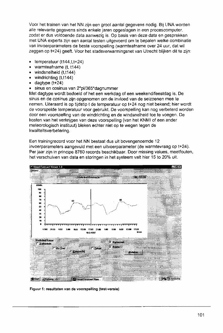
Voor het trainen van het NN zijn een groot aantal gegevens nodig. Bij UNA worden aile relevante gegevens sinds enkele jaren opgeslagen in een procescomputer, zodat er dus voldoende data aanwezig is. Op basis van deze data en gesprekken met UNA experts zijn een aantal testen uitgevoerd om te bepalen welke combinatie van invoerparameters de beste voorspelling (warmteafname over 24 uur, dat wil zeggen op t+24) geeft. Voor het stadsverwarmingsnet van Utrecht blijken dit te zijn:

• temperatuur (t144,t,t+24) • warmteafname (t, t144) • windsnelheid (t,t144) • windrichting (t,t144) • dagtype (t+24) • sinus en cosinus van 2*pi/365*dagnummer Met dagtype wordt bedoeld of het een werkdag of een weekend/feestdag is. De sinus en de cosinus zijn opgenomen om de invloed van de seizoenen mee te nemen. Uiteraard is op tijdstip t de temperatuur op t+24 nog niet bekend; hier wordt de voorspelde temperatuur voor gebruikt. De voorspelling kan nag verbeterd worden door een voorspelling van de windrichting en de windsnelheid toe te voegen. De kosten van het verkrijgen van deze voorspelling (van het KNMI of een ander meteorologisch instituut) bleken echter niet op te wegen tegen de kwaliteitsverbetering.

Een training record voor het NN bestaat dus uit bovengenoemde 12 invoerparameters aangevuld met een uitvoerparameter (de warmtevraag op t+24). Per jaar zijn in principe 8760 records beschikbaar. Door missing values, meetfouten, het verschuiven van data en storingen in het systeem valt hier 15 to 20% uit.

'88 !II

80

10

60

~o

40

30

20

10

11:00 21:00 1:00 5:00 9:00 13:00 11:00 21:80 1:88 5:00 9:80 13:00 11:00 10.2.1991 Uren

Figuur 1: resultaten van de voorspelling (test-versie)

101

102

Vervolgens moet men bepalen of men aile data in een neuraal netwerk stopt of anderscheid gaat maken in meerdere netwerken (een netwerk voor de zome" een voor de winter etc.). Uiteindelijk kan men het NN gaan trainen en testen. In dit project is daar de binnen KEMA ontwikkelde neurale netwerkapplicatie FNS voar gebruikt. Meer details zijn te vinden in [3].

Figuur 1 geeft aan hoe de operator uiteindelijk de resultaten van de voorspelling te zien krijgt (testversie). Links ziet men de actuele en voorspelde waarde van de afgelopen 24 uur, rechts ziet men de voorspelde waarde voor de komende 24 uur. De in de figuur getoonde nauwkeurigheid is voldoende voor bedrijfsvoerings­doeleinden. Leuk detail is dat ook de temperatuurvoorspelling met behulp van een neuraal netwerk gaat worden uitgevoerd. Een nadere beschrijving kan worden gevonden in [3].

Adviessysteem TUNON

Een kolengestookte elektriciteitscentrale heeft een groot aantal regelmogelijkheden. Het is voor de operators dan ook niet eenvoudig om de optimale insteliing te vinden voor diverse kolensoorten. De operator dient bij het optimaliseren te letten op meerdere parameters. Zo moet hij een hoog rendement halen, maar ook zorgen dat de uitstoot van schadelijke stoffen (NOx ernissie) minimaal is. Het veranderen van een instelling leidt vaak tot een verbetering van het rendement, maar ook tot een verhoging van de emissie (wet van behoud van ellende). Om de operators te ondersteunen bij de bedrijfsvoering ontwikkelt KEMA samen met Schelde en de Nederlandse produktiebedrijven een adviessysteem. De naam TUNON staat voor "Thermal behaviour, Unburned carbon and NOx emission Optimized with Neural Networks. Dit systeem adviseert wat de optimale instellingen zijn voor een gegeven situatie. Hart van het systeem is een model van het verbrandingsproces in de ketel. Op basis van dit model bepaalt een optimalisatieprogramma de optimale instellingen, rekening houdend met een groot aantal randvoorwaarden.

Het model van het verbrandingsproces moet van goede kwaliteit zijn. De optimalisatieroutine gebruikt het model om de juiste instellingen te bepalen. Indien het model geen goede beschrijving is van het eigenlijke proces geeft het systeem adviezen die het proces niet tot het optimum voeren. Om de volgende redenen is gekozen om neurale netwerken te gebruiken voor de modellering:

• het proces is sterk nietlineair; neurale netwerken zijn zeer goed in staat om te gaan met nietlineariteit

• het proces heeft veel in en uitvoerparameters; neurale netwerken kunnen omgaan met een groot aantal in en uitvoerparameters

• modellering met conventionele methoden is niet goed mogelijk; mogelijk bieden neurale netwerken een oplossing

De mogelijkheid om fuzzy logic te gebruiken bij de modellering is kort overwogen maar verworpen. Probleem is namelijk dat men de relaties tussen de processen in de ketel empirisch moet modelleren. Gezien het grote aantal in en uitvoerparameters zal dit merkbaar moeilijker zijn dan modellering met neurale netwerken.

TUNON wordt ontwikkeld met de Maasvlaktecentrale van EZH als "pilotplant". Deze centrale be staat uit 2 eenheden van ieder 540 MW. Ter iIIustratie, een zo'n eenheid levert genoeg elektriciteit voor een grote stad.

Bij de start van de ontwikkeling zijn een aantal gesprekken met plantoperators en andere experts van EZH gevoerd. Op deze manier is afgeleid welke parameters een rol spelen bij de modelvorming. De operator beoordeelt de plantperformance op basis van 7 parameters (5 parameters voor het rendement, 2 parameters voor de schadelijk stoffen). Deze 7 uitvoerparameters blijken bepaald te worden door 42 invoerparameters (regelgrootheden en externe omstandigheden). De regelgrootheden (een subset uit de 42 invoerparameters) moeten nu zodanig ingesteld worden dat de 7 uitvoerparameters geoptimaliseerd worden. De optimalisatieroutine maakt gebruik van een NN model om het optimum te bepalen.

Het proces is dus te beschrijven door 42 invoer en 7 uitvoerparameters. Vertaald naar het NN betekent dit dat een leerrecord bestaat uit 49 getallen (42 in, 7 uit). Het procesbewakingssysteem van EZH slaat iedere 10 minuten aile relevante gegevens op. Uit deze gegevens zijn een groot aantal records af te leiden (in principe 6 per uur, oftewel 50.000 per jaar). Het is uiteraard niet mogelijk dergeljjke aantallen records direct toe te voeren aan het NN. Sommige records hebben ontbrekende waarden of bevatten meetfouten, een aantal records beschrijft overgangssituaties. sommige records bevatten geen nieuwe informatie etc. Er zijn een aantal technieken beschikbaar om de ontwikkelaar te ondersteunen bij de datavalidatie. Deze technieken zijn niet altijd bruikbaar. Ais een meter op 9999 staat is duidelijk wat er aan de hand is. Het bepalen van wegdriftende of slecht geijkte meters is echter minder triviaal. Inbreng van de EZH experts is dan ook onmisbaar bij het valideren van de gegevens.

Nadat een leer en testset van goede kwaliteit zijn samengesteld is het NN getraind, deze keer met een commercieel verkrijgbaar NN pakket. Afhankelijk van het aantal datasets en de in en uitvoerparameters doet men een schatting voor het aantal neuronen. In dit geval blijkt een standaard type NN met 2 verborgen lagen met ieder circa 20 neuronen een goed resultaat te geven. Een meer gedetailleerde beschrijving van de resultaten kan worden gevonden in [4].

Zoals gezegd wordt het NN gebruikt om de optimale instelling van het proces te bepalen. Er zijn echter situaties waarin het NN geen goed model vormt van het proces, denk aan een bedrijfsvoeringssituatie die totaal niet lijkt op de situaties die in de leerset zijn voorgekomen. In dergelijke gevallen geeft het NN toch een antwoord, hoewel het eigenlijk buiten zijn werkgebied is. Ais gebruiker van NN wit je dat het NN dergelijke situaties zelf aangeeft, met de huidige typen netwerken is dit nog niet goed mogelijk. Hier ligt een uitdaging voor de universiteiten om een NN te ontwikkelen dat bij iedere uitvoer een indruk geeft van de betrouwbaarheid van het resultaat.

103

104

Gebruik neurale netwerken

In dit artikel is het gebruik van NN aan de hand van twee voorbeelden gelliustreerd. Bij het werken met NN moet men vooral aandacht besteden aan het bepalen van de juiste in en uitvoerparameters en het verkrijgen van een goede representatieve leer en testset. De stelling "garbage in ::: garbage out" geldt ook bij het trainen van NN; een NN moet getraind worden met goede kwaliteit gegevens en is pas daama relatief robuust voor verstoringen/foute invoerdata. Het verkrijgen van voldoende data is vaak een probleem. Er zijn minimaal enkele 100e datasels nodig. In de praktijk blijkt een aanzienlijk percentage (15%60%) van de aangeleverde data weg te vallen door diverse oorzaken. Het verkrijgen van voldoende variatie in de datasets is belangrijk. De leerset moet representatief zijn voor het hele systeem. Er zjjn verschillende technieken om de ontwikkelaar te ondersteunen bij deze eisen.

Het is niet nodig grote investeringen in NN programma's te doen. Er zijn voldoende pakketten verkrijgbaar onder NLG 10.000 die voldoende funktionaliteit te hebben voor een breed scala aan toepassingen. Besteed niet teveel tijd aan het bepalen van het optimale aantal neuronen; Met enig gevoel en ervaring kan men snel een voldoende resultaat verkrijgen (20/80 regel, met 20% van de inspanning bereikt men 80% van het maximaal haalbare resultaat).

Een NN is niet iets dat "turn key" geleverd kan worden. Voor een succesvolle toepassing is binnen het projectteam zowel kennis van het proces als NN nodig. De in deze voordracht genoemde toepassingen zijn dan ook tot stand kunnen komen dankzij de inzet van het UNA respectievelijk EZH projectteam.

Literatuur

[1] Artificial Neural Networks applied to power systems; A.G. Jongepier, dissertatie, 1996, KEMA, Arnhem

[2] Cigre TF 380606 on ANN applications for Power Systems, D. Niebur (convenor). Neural Network Applications in Power Systems. Int. Journal of Engineering Intelligent Systems, December 1993

[3] Application of NN for prediction of demand in a district heating system, R. Frenken, S. Landman, M. Vermeulen en H. Oort, DAlDSM96, Oktober 1996, Wenen.

[4] Development of an advisory system based on a neural network for the operation of a coal fired power plant, R. Frenken, C. Rozendaal, H. Dijk en P. Knoester, ICANN96, July 1996, Bochum

EEN GAT IN DE BEGROTING?

(0.1 Stichting Professor Gelissenfonds

Bestuur mw. drs. M.E. van Bodengraven prof.ir W.L. Kling prof.dr.ir. p.eT van der Laan Ir. O. Ongklehong ir. F. de Ruiter (voorzitter) ir. H.G. Smits

Stichting "PROFESSOR GELISSENFONDS" kan helpen!

De Stichting "Professor Gelissenfonds" verstrekt jaarlijks financiele bijdragen aan activiteiten van studenten en studentenverenigingen.

Bij het beoordelen van aanvragen gaat het bestuur uit van de doelstelling van het fonds:

"Het leveren van een bijdrage aan de onfwikke/ing, de toepassing en de verspreiding van kennis op het gebied van de opwekking, conversie en toepassing van elektrische energie."

Het gaat daarbij in de eerste plaats om activiteiten die door studenten zelf georganiseerd en uitgevoerd worden. Ook moet er een duidelijk verband zijn tussen het vakgebied "energie" en de te ondersteunen activiteit. Voorbeelden van ondersteuning door het fonds zijn: studiereizen en excur­sies, bijdragen aan de studieverenigingen en de disputen, bijzondere onder­zoeks- en afstudeeropdrachten en/of stages.

In de Stichting werken de elektriciteitsproduktie- en distributiebedrijven (verenigd in de VDEN - de vereniging van directeuren van elektriciteitsbedrij­ven) en de industrie samen.

Bij aanvragen voor ondersteuning moet voldoende documentatie, waaronder een begroting van baten en lasten, worden overlegd. Achteraf dienen een verslag en een financiele verantwoording te worden gepresenteerd.

Aanvragen voor bijdragen zijn te richten aan: Bestuur Professor Gelissen­fonds t.a.v. H.F.M. Zewald, secretariaat.

STICHTING PROFESSOR GELISSENFONDS

Secretariaat: Utrechtseweg 310, 6812 AR Amhem, Postbus 9035,6800 ET Amhem, Nederland. Telefoon (026) 3 56 28 98. Telefax (026) 4 42 90 93. ABN+AMRO Bank NV Amhem, rekeningnummer 53.44.25.771. Handelsreglster nummer S 49020. Kamer van Koophandel en Fabrieken voor Midden-Geiderland

106

Biegraf4e

Nikolay Petkov is professor of computer sci.ence. YiSlding a chair of parallel computing at/the University of SrQnII'l;en in the Netherlands. He is also the head of the ·Centlte:for Hi§tl Perfermanee~mputing of the same university. Pfe got his D.S~,llil}r.sc.te_n.) degree

in Computer Engineering Informatlonstectmik) from Dfesden University at Te~nQ'ogy. Prior to joinI~;;the ComJ1;ltingScience Department of the University of Groningen, hetleld researCfipositions,aMbeUniverlity of Wuppertal, the Univ&fE$ity of Erlangen-Num berg , the"AcaaemvQfif8ciences of GDR in Berlin, the Academy of Scteflres,of S.lovacia in Bratisla!\ta ana Dresden University of Technology.

Nikolay Petkov is the author ofthe books Systolische AlgoFithmen und Arrays (~rtin: A.kademie"~~j 1989),ancj~J~JoUc Parallel ProceSSing Amsterdam: North.;Hollan~!I EI~~i~~ScL Pubt.,1~S~frend of further 70 scie:nJific papers; Fie also holds sevefalpatents.He is member-of theeditorialb~t\lrds of ~ journals Plarallef Computing (Nc:lpth-Ra[JiiJl"lqlr~rallelAI~~liilltims and Applications (Gordon and Breach} and ReaJ-T~'ma!!Jing (Academic 'Press) and of a number of Dutch and international profeSS[~Ral bodies. In 1989 he has been awarded an Alexander von Fiumboldt scholarshij'iJsf the Federal Republic of Germany.

This Is a reprint of: N. Petkovand P. Kruizinga, "Computational models of visual neurons specialised in the detection of periodic and aperiodic oriented visual stimuli: bar and grating cells", Biological Cybernetics, 1997,76(2):83-96. © Springer·Veriag 1997.

Computational models of visual neurons specialised in the detection of periodic and

aperiodic oriented visual stimuli: bar and grating cells

N. Petkov and P. Kruizinga, Centre for High Performance Computing and Institute of

Mathematics and Computing Science University of Groningen P.O. Box 800,9700 AV Groningen

Email: petkov@cs.rug.nl.peterkr@cs.rug.nl

Abstract: Computational models of periodic- and aperiodic-pattern selective cells, also called grating and bar cells, respectively, are proposed. Grating cells are found in areas V1 and V2 of the visual cortex of monkeys and respond strongly to bar gratings of a given orientation and periodicity but very weakly or not at all to single bars. This non-linear behaviour, which is quite different from the spatial frequency filtering behaviour exhibited by the other types of orientation selective neurons such as the simple cells, is incorporated in the proposed computational model by using an AND-type non-linearity to combine the responses of simple cells with symmetric receptive field profiles and oppOSite polarities. The functional behaviour of bar cells, which are found in the same areas of the visual cortex as grating cells, is less well explored and documented in the literature. In general, these cells respond to single bars and their responses decrease when further bars are added to form a periodic pattern. These properties of bar cells are implemented in a computational model in which the responses of bar cells are computed as thresholded differences of the responses of corresponding complex (or simple) cells and grating cells. Bar and grating cells seem to play complementary roles in resolving the ambiguity with which the responses of simple and complex cells represent oriented visual stimuli, in that bar cells are selective only for form information as present in contours and grating cells only respond to oriented texture information. The proposed model is capable of explaining the results of neurophysiological experiments as well as the psychophysical observation that the perception of texture and the perception of form are complementary processes.

Keywords: Visual cortex, computational model, texture, bars, contours, periodic and aperiodic stimuli, orientation, spatial frequency, simple cells, complex cells, bar cells, grating cells.

107

108

1 Introduction

The discovery of orientation selective cells in the primary visual cortex of monkeys almost forty years ago and the fact that most of the neurons in this part of the brain are of this type [14, 151 have triggered a wave of research activities in the subsequent years, aimed at a more precise, quantitative description of the functional behaviour of such cells. Questions of what the optimal stimuli -- bars and edges or gratings -- for this type of cells are and whether they carry out bar and edge detection or local frequency analysis gained considerable attention in the literature [2, 8, 9, 21, 36, 37]. In the meantime functional descriptions and adequate computational models of the main classes of orientation selective visual neurons such as the simple and complex cells have been proposed and the above questions have received satisfactory answers.

Simple cells can be modelled by linear filters followed by half-wave rectification [3, 13, 20, 22, 27]. Their orientation and spatial frequency selectivity can be explained by the specific kind of linear filtering involved. The space-domain impulse responses of these filters can quite well be approximated by two-dimensional Gabor functions [7, 17] and, knowing the properties of these functions, it is easy to understand why this kind of filters act as local edge and bar detectors [30]. The two-dimensional spatial frequency response of such a filter is represented by two Gaussian functions whose centres are symmetrically displaced from the centre of the spatial frequency domain and this explains the orientation and spatial frequency selectivity of the filter and its strong response to gratings of appropriate orientation and periodicity. The above facts, combined with the locality of these filters, explain why they act as local spatial frequency analysers and, at the same time, as local edge and bar detectors. Complex cells behave similarly, but need more intricate modelling which includes three stages: linear filtering, rectification and local spatial summation [26, 28, 33, 34, 35].

The focusing of the attention of the research community on the dilemma edge/bar detection vs. local frequency analysis properties of simple cells may have occluded the functional diversity in the rather broad class of all orientation selective cells. Relatively recently Von der Heydt et al. [38, 39] reported on the discovery of a new type of orientation selective neurons in areas V1 and V2 of the visual cortex of monkeys which they called grating cells. Similarly to other orientation selective neurons, such as Simple, complex and hyper-complex cells, grating cells respond vigorously to a grating of bars of appropriate orientation, position and periodicity. In contrast to other orientation selective cells, grating cells respond very weakly or not at all to single bars, this means, bars which are isolated and do not make part of a grating. This behaviour of grating cells cannot be explained by linear filtering followed by half-wave rectification as in the case of simple cells, neither can it be explained by three-stage models of the type used for complex cells. Most grating cells start to respond when a grating of a few bars (2 to 5) is presented. In most cases the response rises linearly with the number of additional bars up to a given number (4 to 14) after which it quickly saturates and the addition of new bars to the grating causes the response to rise only slightly or not at all and in some cases even to decline. Similarly, the response rises with the length of the bars up to a given length after which saturation and in some cases inhibition is observed. The responses to moving gratings are unmodulated and do not depend on the direction of movement. The dependence of the response on contrast shows a switching characteristic, in that turn-on and saturation contrast values lie pretty close: the most sensitive grating

cells start to respond at a contrast of 1 % and level off at 3%. In general, grating cells are more selective than simple cells 1, having spatial frequency bandwidths in the range of 0.4-1.4 octaves, with median 1 octave and orientation bandwidth of about 20°.

During their research on grating cells, Von der Heydt et al. also found other cells which responded to Single bars but not at all to square-wave gratings of any periodicity [391. More generally, this type of cells, which we call bar cells in the following, respond most strongly to Single bars and their responses decrease with the addition of further parallel bars to make a grating. In previous studies Schiller et al. [32] also found many cells in area V1 which responded strongly to single bars and edges but did not respond to sine-wave gratings. Blakemore and Tobin [5] measured the response of a 'complex' cell to a white bar of optimal orientation, position and size in the presence of a bar grating covering the area outside a circle which was somewhat larger than the region in which the cell responded to the bar stimulus. They observed an inhibition effect due to the grating. This effect was strongest when the grating had the same orientation as the optimal bar stimulus. In this case the response of the cell was reduced to the level of spontaneous activity. The inhibition

. effect of the grating decreased with the deviation of its orientation from the optimal orientation of the bar stimulus. One may wish to think of this cell as a bar cell similar to the cells described by Schiller et al. and Von der Heydt et al. Unfortunately, the properties of this class of cells are not suffiCiently well investigated and reported in the literature.

The above properties suggest that the primary role of grating cells is to detect periodicity in oriented patterns, ignoring other details (such as contrast). On the other hand, their higher specialisation and relatively narrow bandwidths cause them to be activated by natural visual stimuli relatively rarely, compared to other orientation selective cells. The higher specialisation of bar cells as compared to other orientation selective cells raises similar questions. Therefore, the roles of bar and grating cells need to be clarified in order to get better inSights into the structure of the visual system and the role of functional speCialisation. The approach to this problem adopted in this study is a computational one: computational models of bar and grating cells are proposed and used to simulate their activity. On the basis of the results we draw conclusions about the possible role of bar and grating cells in the visual system.

The paper is organised as follows: in Section 2 computational models of both simple and complex cells are briefly introduced. These models are well-known from the literature but since they make part of the models of bar and grating cells, they are included in the paper for ease of reference and clarity of parametrisation. A computational model of grating cells is given in Section 3. In the same section, we present the results of some computer simulations of modelled grating cells. Furthermore grating cell operators are compared with complex cell operators with respect to the detection and segmentation of texture. In Section 4 a computational model of bar cells is introduced and the results of computer simulations of such cells, which explain neurophysiological observations are given. Perceptual experiments are presented and an explanation of the observed phenomena is provided based on the simulations of grating and bar cells using the proposed computational models. In

I Simple cell spatial frequency bandwidths at half response vary in the range 0.4-2.6 octaves with median 1.4 octave; their median orientation bandwidth is about 400 [10].

109

110

Section 5 we summarise the results of the study and draw some conclusions about the role which grating and bar cells play in the processing of visual information.

2 Preliminary - computational models of simple and complex cells

Bar and grating cells are found in the same cortical area (V1) as simple and complex cells and similarly to simple and complex cells show orientation selectivity. On the other hand they show a more complex non-linear behaviour and a sharper orientation and spatial frequency tuning. These facts suggest that bar and grating cells receive input from simple or complex cells and below we propose a model in which the responses of simple and complex cells are used to compute the responses of bar and grating cells. This is similar to the idea that complex cells may receive inputs from simple cells [16], an idea which explicitly or implicitly is used in most complex cell models. Since Simple cells playa substantial role in the following. we first briefly introduce a computational model of this type of cells. The response r of a simple cell which is characterised by a receptive field function g(x,y) to a luminance distribution image f(x,y),(x,y) eO, is computed as follows (0 -visual field domain):

r = x(IIf(x,y) g(x,y) dxdy) n

where X is the Heaviside step function (X(z) = 0 for z < 0, X(z) = z for z ~ 0). Below we extend this Simple model with a local contrast compensation.

(1)

We use the following family of two-dimensional Gabor functions [7] to model the spatial summation properties of simple cells2

: where the arguments x and y specify the position of a light

_ (x,1+,ly,2) x' g~.I1.l.a.9'(X,y) = e 2,,2 cos(27l' A + <p)

x' = (x - q)cos8 - (y - 1J)sin 8 (2)

y'= (x - q)sin8 +(y -1J)cos8

impulse in the visual field and q ,1J, (J' • r ,8 and <p are parameters as follows:

The pair (~,1J), which has the same domain 0 as the pair(x,y) , specifies the centre of a receptive field within the visual field. The standard deviation (J' of the Gaussian factor determines the (linear) size of the receptive field. Its eccentricity and herewith the eccentricity of the receptive field ellipse is determined by the parameter r , called the spatial aspect ratio. It has been found to vary in a limited range of 0.23 < r < 0.92 [17]. The value r = 0.5 is used in our simulations and, since this value is constant, the parameter r is not used to index a receptive field function.

2 Our modification of the parametrisation used in [7] takes into account the restrictions found in experimental data.

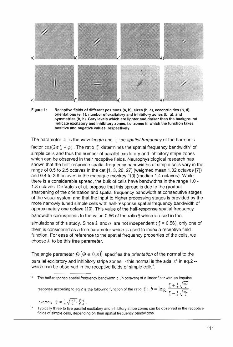
Figure 1: Receptive fields of different positions (a, b), sizes (b, c), eccentricities (b, d), orientations (e, f), number of excitatory and inhibitory zones (b, g), and symmetries (b, h). Gray levels which are lighter and darker than the background indicate excitatory and inhibitory zones, i.e. zones in which the function takes positive and negative values, respectively.

The parameter A is the wavelength and ± the spatial frequency of the harmonic

factor cos(2Jr f + cp) . The ratio T determines the spatial frequency bandwidth3 of simple cells and thus the number of parallel excitatory and inhibitory stripe zones which can be observed in their receptive fields. Neurophysiological research has shown that the half-response spatial-frequency bandwidths of simple cells vary in the range of 0.5 to 2.5 octaves in the cat [1, 3, 20, 27] (weighted mean 1.32 octaves [7]) and 0.4 to 2.6 octaves in the macaque monkey [10] (median 1.4 octaves). While there is a considerable spread, the bulk of cells have bandwidths in the range 1.0 -1.8 octaves. De Valois et al. propose that this spread is due to the gradual sharpening of the orientation and spatial frequency bandwidth at consecutive stages of the visual system and that the input to higher processing stages is provided by the more narrowly tuned simple cells with half-response spatial frequency bandwidth of approximately one octave [10]. This value of the half-response spatial frequency

bandwidth corresponds to the value 0.56 of the ratio T which is used in the

simulations of this study. Since A and (J' are not independent ( T = 0.56), only one of

them is considered as a free parameter which is used to index a receptive field function . For ease of reference to the spatial frequency properties of the cells, we choose A to be this free parameter.

The angle parameter e (e E [ 0, Jr)) specifies the orientation of the normal to the

parallel excitatory and inhibitory stripe zones -- this normal is the axis Xl in eq .2 -­which can be observed in the receptive fields of simple cells4

•

3 The half-response spatial frequency bandwidth b (in octaves) of a linear filter with an impulse

Q. + ~ rIrri c; b __ 10 ). ;r \/2 response according to eq.2 is the following function of the ratio 1" : g

2 Q. _ ~ rJ;;2" ). H \/ {

Inversely Q. = ~Jln2 . ~ ' A H 2 2b _\ "

, Typically three to five parallel excitatory and inhibitory stripe zones can be observed in the receptive fields of simple cells, depending on their spatial frequency bandwidths.

111

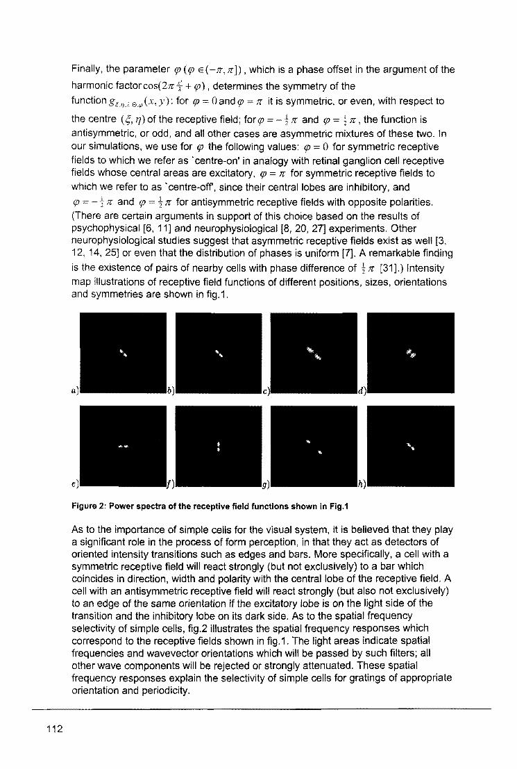
112

Finally, the parameter cp (cp E (-:rr,:rr]) , which is a phase offset in the argument of the

harmonic factorcos(2:rrf + cp), determines the symmetry of the

function K:'1,;.e,q> (x, y): for cp 0 and cp =:rr it is symmetric, or even, with respect to

the centre (~, rJ) of the receptive field; for cp = t:rr and cp = t:rr , the function is antisymmetric, or odd, and all other cases are asymmetric mixtures of these two. In our simulations, we use for cp the following values: cp = 0 for symmetric receptive fields to which we refer as 'centre-on' in analogy with retinal ganglion cell receptive fields whose central areas are excitatory, cp =:rr for symmetric receptive fields to which we refer to as 'centre-off, since their central lobes are inhibitory, and

cp i:rr and cp = t:rr for antisymmetric receptive fields with opposite polarities. (There are certain arguments in support of this choice based on the results of psychophysical [6, 11] and neurophysiological [8, 20, 27] experiments. Other neurophysiological studies suggest that asymmetric receptive fields exist as well [3, 12, 14, 25] or even that the distribution of phases is uniform [7]. A remarkable finding

is the existence of pairs of nearby cells with phase difference of t:rr [31].) Intensity map illustrations of receptive field functions of different positions, sizes, orientations and symmetries are shown in fig.1.

a)

e

Figure 2: Power spectra of the receptive field functions shown in Fig.1

As to the importance of simple cells for the visual system, it is believed that they play a significant role in the process of form perception, in that they act as detectors of oriented intenSity transitions such as edges and bars. More specifically, a cell with a symmetric receptive field will react strongly (but not exclusively) to a bar which coincides in direction, width and polarity with the central lobe of the receptive field. A cell with an antisymmetric receptive field will react strongly (but also not exclusively) to an edge of the same orientation if the excitatory lobe is on the light side of the transition and the inhibitory lobe on its dark side. As to the spatial frequency selectivity of simple cells, fig.2 illustrates the spatial frequency responses which correspond to the receptive fields shown in fig.1. The light areas indicate spatial frequencies and wavevector orientations which will be passed by such filters; all other wave components will be rejected or strongly attenuated. These spatial frequency responses explain the selectivity of simple cells for gratings of appropriate orientation and periodiCity.

Using the above parametrisation, one can compute the response s~.T/,).,e,ffJ of a simple

cell modelled by a receptive field function g~'T/.)..e'f1(x,y) to an input image with

luminance distribution!(x,y) as follows:

First, an integral

r~.T/.).,e,tp = II!(x,y) g~.T/,)..e.f1(x,y) dxdy n

(3)

is evaluated in the same way as if the receptive field functiong~,T/,).,e'f1(x,y) were the response of a linear system. In order to normalise the simple cell response with respect to the contrast of the input image, r~.T/.).,e'f1 is divided by the average gray

level within the receptive field. The averagea~.T/.). is computed using the Gaussian

factor of the function g~,T/,)..e.f1 (x, y) :

(X_{)l+r2 (p_q)1

a~,T/,). = II !(x,y) e--1;;i- dxdy n

(4)

The ratio r;;~q'A,e, .. is proportional to the local contrast within the receptive field of a cell. ~,q,).

In order to obtain a contrast response function similar to the ones measured on real cells, we use the hyperbolic ratio function to calculate the simple cell response from the ratio r{~q,J.,e, ...

{,q,'

if a =0

otherwise (5)

where Rand C are the maximum response level and the semi-saturation constant, respectively.

In the following we also need a computational model of complex cells for a comparison of their computed responses to oriented texture with the computed responses of grating cells and as input to bar cell operators. We use the following model of complex cells:

(6)

which represents weighted spatial summation of the quadrature responses of simple cells of the same preferred orientation e and spatial frequency 1:, but with receptive

field centres (c;', 'f}') spread within the neighbourhood of the receptive field

centre (c;, 'f}) of the complex cell. The size of this neighbourhood is determined by the

113

114

parameter crt which we choose to be two times greater than the respective parameter cr in the simple cell model, cr'= 2cr. We have to note that this model describes only one type of cells in the rather broad class of complex cells. Complex cells of this type will respond to edges and bars of appropriate orientation within their receptive fields, regardless of their exact position and polarity (Le. there is no phase modulation). This model is sufficient for the purpose of this study.

3 Grating cells

3.1 Computational model Von der Heydt et al. [38] have proposed a model of grating cells in which the activities of displaced semi-linear units of the simple cell type are combined by an AND-type non-linearity to produce grating cell activity. While the simple model they propose reacts to gratings of appropriate orientation and periodicity and does not react to single bars, it will also react to a number of stimuli to which grating cells would not respond, for instance a bar and an edge parallel to it. Their simple model does also not account for correct spatial frequency tuning -~ it will for instance react not only to the fundamental spatial frequency, but also to all multiples of it -- and the spatial summation properties of grating cells. We therefore give an alternative model of grating cells which is aimed at reproducing all their properties which are known from neurophysiological experiments.

Our model of grating cells consists of two stages [19]. In the first stage, the responses of so-called grating subunits are computed using as input the responses of centre-on and centre-off simple cells with symmetrical receptive fields. The model of a grating subunit is conceived in such a way that the unit is activated by a set of three bars with appropriate periodicity, orientation and position. In the next, second stage, the responses of grating subunits of a given preferred orientation and periodicity are summed together within a certain area to compute the response of a grating cell. This model is next explained in more detail:

A quantity q q.1I.e•1 • called the activity of a grating subunit with position (~, 17) , preferred

orientation E> and preferred grating periodicity A, is computed as follows:

= {I if'v'n, n E {-3 ... 2}, M q,1I.e•1,n ~ pM :.q.e.l

Qq.lI,e.l 0 if3n, n E {-3. .. 2}, M q•lI,e.l.1I <pM:.~.e.l (7)

where p is a threshold parameter with a value smaller than but near 1 (e.g. p = 0.9)

and the auxiliary quantities M q.1I.e•1•1I and M q,,,.e.l.1I are computed as follows:

M q•lI.e ,l,n = max {Sq""'.e.lo9'n , ~', 17': n teosE>::;; (~'-~ < (n + l)tcosE>,

n t sinE> ::;; (17 '-17) < (n + 1) t sinE>, (8)

{o n = -3 -11 , , }

rp = n 1t n = -2,0,2

and

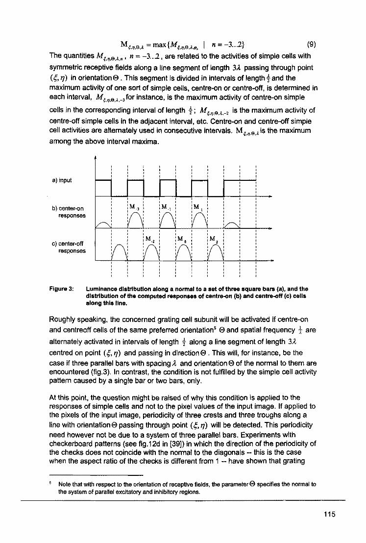
M~'11,9,A. = max{Mi ,I1,9,l,fJ. I n = -3 ... 2} (9)

The quantities M ~.11,9,l.n' n = -3 ... 2 , are related to the activities of simple cells with

symmetric receptive fields along a line segment of length 3A passing through point (~. 17) in orientation E>. This segment is divided in intervals of length 1 and the maximum activity of one sort of simple cells, centre-on or centre-off, is determined in each interval, Mi.I1.9.l.-3 for instance, is the maximum activity of centre-on simple

cells in the corresponding interval of length 1; M i ,f1,9,l.-2 is the maximum activity of centre-off simple cells in the adjacent interval, etc. Centre-on and centre-off simple cell activities are alternately used in consecutive intervals. M i,l1.S,l is the maximum among the above interval maxima.

a) input

b) center-on responses

c) center-off responses

Figure 3: Luminance distribution along a normal to a set of three square bars (a), and the distribution of the computed responses of centre-on (b) and centre-off (c) cells along this line.

Roughly speaking, the concerned grating cell subunit will be activated if centre-on and centreoff cells of the same preferred orientationS E> and spatial frequency ± are

alternately activated in intervals of length 1 along a line segment of length 3A

centred on point (~, 17) and passing in directionE>. This will, for instance, be the case if three parallel bars with spaCing A and orientation E> of the normal to them are encountered (fig.3). In contrast. the condition is not fulfilled by the simple cell activity pattern caused by a single bar or two bars, only.

At this point, the question might be raised of why this condition is applied to the responses of simple cells and not to the pixel values of the input image. If applied to the pixels of the input image, periodicity of three crests and three troughs along a line with orientationE> passing through point (~, 1]) will be detected. This periodicity need however not be due to a system of three parallel bars. Experiments with checkerboard patterns (see fig.12d in [39]) in which the direction of the periodicity of the checks does not coincide with the normal to the diagonals -- this is the case when the aspect ratio of the checks is different from 1 -- have shown that grating

5 Note that with respect to the orientation of receptive fields, the parameterE> specifies the normal to the system of parallel excitatory and inhibitory regions.

115

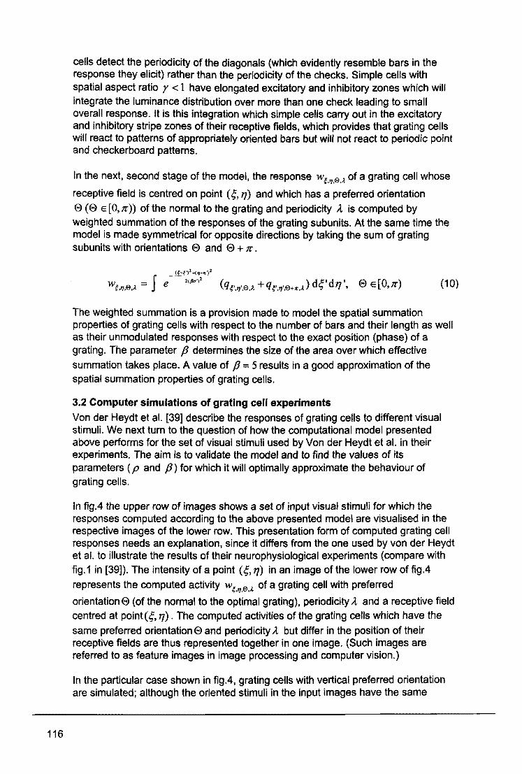
116

cells detect the periodicity of the diagonals (which evidently resemble bars in the response they elicit) rather than the periodicity of the checks. Simple cells with spatial aspect ratio r < 1 have elongated excitatory and inhibitory zones which will integrate the luminance distribution over more than one check leading to small overall response. It is this integration which simple cells carry out in the excitatory and inhibitory stripe zones of their receptive fields, which provides that grating cells will react to patterns of appropriately oriented bars but will not react to periodic point and checkerboard patterns.

In the next, second stage of the model, the response W',l1.@,..t of a grating cell whose

receptive field is centred on point (~, 1]) and which has a preferred orientation

0(0 e [0, n» of the normal to the grating and periodicity A. is computed by weighted summation of the responses of the grating subunits. At the same time the model is made symmetrical for opposite directions by taking the sum of grating subunits with orientations 0 and 0 + n .

0e[0,n) (10)

The weighted summation is a provision made to model the spatial summation properties of grating cells with respect to the number of bars and their length as well as their unmodulated responses with respect to the exact position (phase) of a grating. The parameter P determines the size of the area over which effective

summation takes place. A value of P = 5 results in a good approximation of the spatial summation properties of grating cells.

3.2 Computer simulations of grating cell experiments Von der Heydt et al. [39] describe the responses of grating cells to different visual stimuli. We next turn to the question of how the computational model presented above performs for the set of visual stimuli used by Von der Heydt et al. in their experiments. The aim is to validate the model and to find the values of its parameters (p and P) for which it will optimally approximate the behaviour of grating cells.

In figA the upper row of images shows a set of input visual stimuli for which the responses computed according to the above presented model are visualised in the respective images of the lower row. This presentation form of computed grating cell responses needs an explanation, since it differs from the one used by von der Heydt et al. to illustrate the results of their neurophysiological experiments (compare with

fig.1 in [39]). The intensity of a point (~, 1]) in an image of the lower row of figA

represents the computed activity W'.l1.e.A of a grating cell with preferred

orientation 0 (of the normal to the optimal grating). periodicity A. and a receptive field

centred at point (~, 1]). The computed activities of the grating cells which have the

same preferred orientation e and periodicity A. but differ in the position of their receptive fields are thus represented together in one image. (Such images are referred to as feature images in image processing and computer vision.)

In the particular case shown in figA, grating cells with vertical preferred orientation are simulated; although the oriented stimuli in the input images have the same

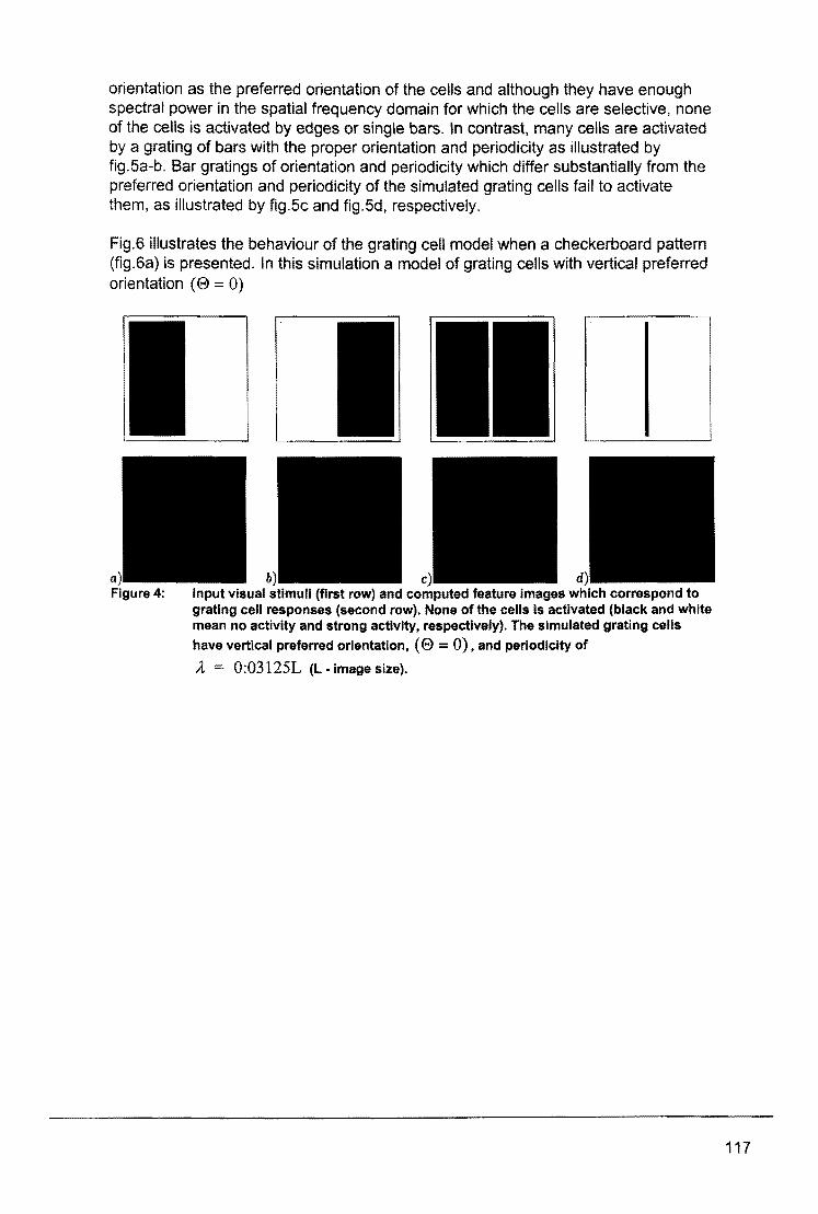
orientation as the preferred orientation of the cells and although they have enough spectral power in the spatial frequency domain for which the cells are selective, none of the cells is activated by edges or single bars. In contrast, many cells are activated by a grating of bars with the proper orientation and periodicity as illustrated by fig.5a-b. Bar gratings of orientation and periodicity which differ substantially from the preferred orientation and periodicity of the simulated grating cells fail to activate them, as illustrated by fig.5c and fig.5d, respectively.

Fig.6 illustrates the behaviour of the grating cell model when a checkerboard pattern (fig.6a) is presented. In this simulation a model of grating cells with vertical preferred orientation (8 = 0)

a ~ Figure 4: Input visual stimuli (first row) and computed feature Images which correspond to

grating cell responses (second row). None of the cells is activated (black and white mean no activity and strong activity, respectively). The simulated grating cells

have vertical preferred orientation, (8 = 0), and periodicity of

A 0:03125L (L - image size).

117

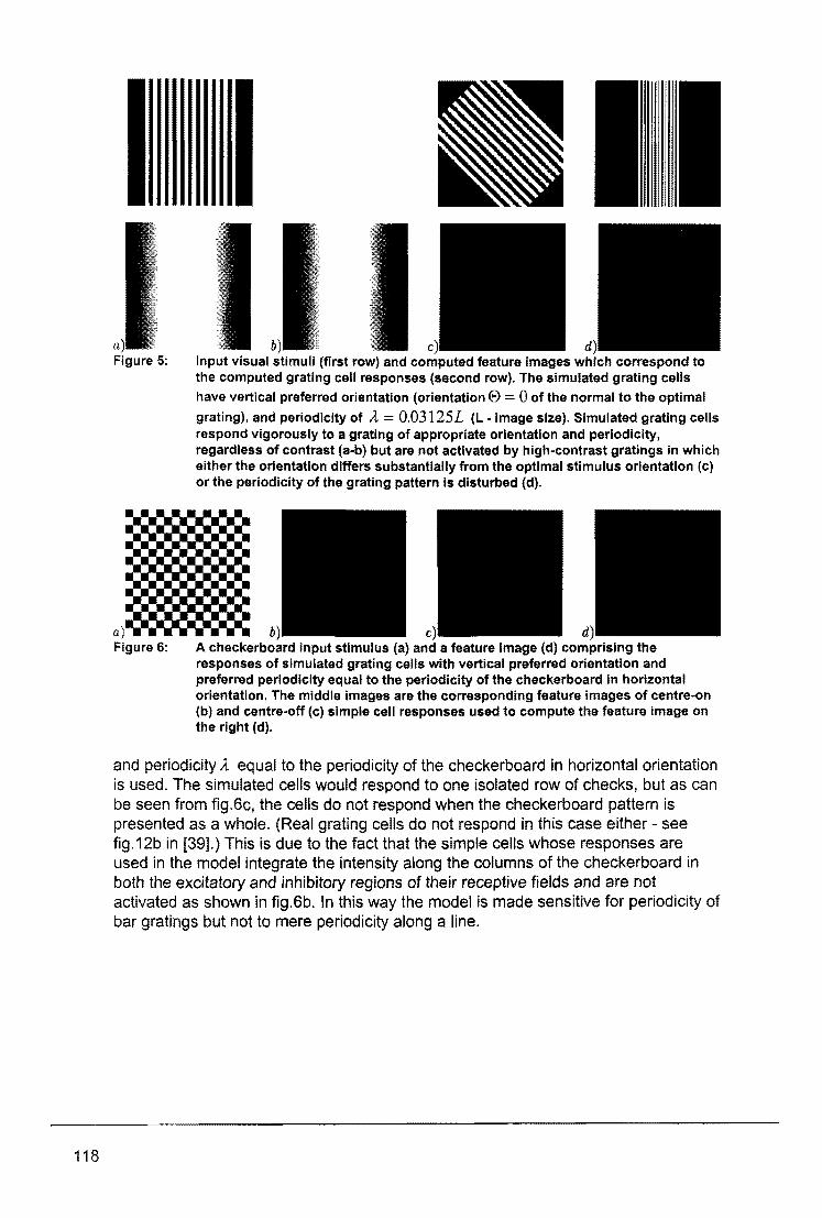
118

a Figure 5:

b) Input visual stimuli (first row) and computed feature images which correspond to the computed grating cell responses (second row). The simulated grating cells

have vertical preferred orientation (orientation 0 == 0 of the normal to the optimal

grating), and periodicity of A = 0.03125L (L - image size). Simulated grating cells respond vigorously to a grating of appropriate orientation and periodicity, regardless of contrast (a-b) but are not activated by high-contrast gratings in which either the orientation differs substantially from the optimal stimulus orientation (c) or the periodicity of the grating pattern is disturbed (d).

• • • • • • • • • • • • • • • • • • • a)

Figure 6:

•

• •

• • A checkerboard input stimulus (a) and a feature image (d) comprising the responses of simulated grating cells with vertical preferred orientation and preferred periodicity equal to the periodicity of the checkerboard in horizontal orientation. The middle images are the corresponding feature images of centre-on (b) and centre-off (c) simple cell responses used to compute the feature image on the right (d).

and periodicity A equal to the periodicity of the checkerboard in horizontal orientation is used. The simulated cells would respond to one isolated row of checks, but as can be seen from fig.6c, the cells do not respond when the checkerboard pattern is presented as a whole. (Real grating cells do not respond in this case either - see fig.12b in [39].) This is due to the fact that the simple cells whose responses are used in the model integrate the intensity along the columns of the checkerboard in both the excitatory and inhibitory regions of their receptive fields and are not activated as shown in fig.6b. In this way the model is made sensitive for periodicity of bar gratings but not to mere periodicity along a line.

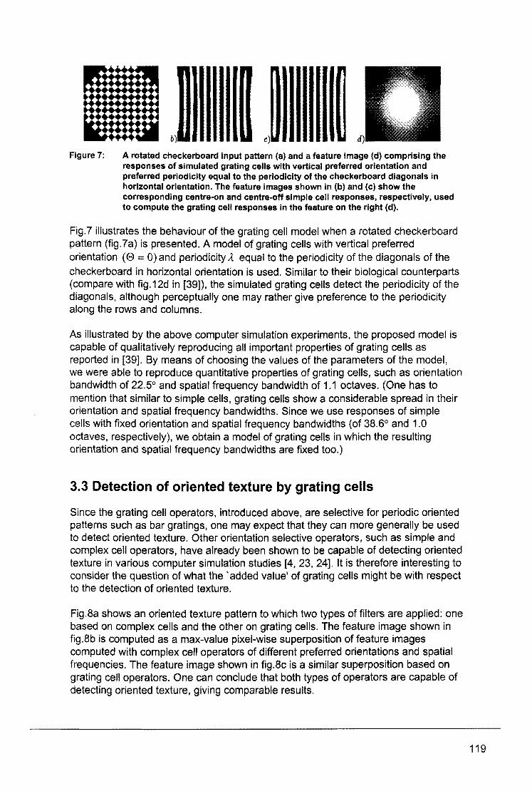
c)

Figure 7: A rotated checkerboard input pattern (a) and a feature image (d) comprising the responses of simulated grating cells with vertical preferred orientation and preferred periodicity equal to the periodicity of the checkerboard diagonals in horizontal orientation. The feature images shown in (b) and (c) show the corresponding centre-on and centre-off simple cell responses, respectively, used to compute the grating cell responses in the feature on the right (d).

Fig.? illustrates the behaviour of the grating cell model when a rotated checkerboard pattern (fig.?a) is presented. A model of grating cells with vertical preferred orientation (0 = 0) and periodicity A equal to the periodicity of the diagonals of the checkerboard in horizontal orientation is used. Similar to their biological counterparts (compare with fig.12d in [39]), the simulated grating cells detect the periodicity of the diagonals, although perceptually one may rather give preference to the periodicity along the rows and columns.

As illustrated by the above computer simulation experiments, the proposed model is capable of qualitatively reproducing all important properties of grating cells as reported in [39]. By means of choosing the values of the parameters of the model, we were able to reproduce quantitative properties of grating cells, such as orientation bandwidth of 22.50 and spatial frequency bandwidth of 1.1 octaves. (One has to mention that similar to simple cells, grating cells show a considerable spread in their orientation and spatial frequency bandwidths. Since we use responses of simple cells with fixed orientation and spatial frequency bandwidths (of 38.60 and 1.0 octaves, respectively), we obtain a model of grating cells in which the resulting orientation and spatial frequency bandwidths are fixed too.)

3.3 Detection of oriented texture by grating cells

Since the grating cell operators, introduced above, are selective for periodic oriented patterns such as bar gratings, one may expect that they can more generally be used to detect oriented texture. Other orientation selective operators, such as simple and complex cell operators, have already been shown to be capable of detecting oriented texture in various computer simulation studies [4, 23, 24]. It is therefore interesting to consider the question of what the' added value' of grating cells might be with respect to the detection of oriented texture.

Fig.8a shows an oriented texture pattern to which two types of filters are applied: one based on complex cells and the other on grating cells. The feature image shown in fig.8b is computed as a max-value pixel-wise superposition of feature images computed with complex cell operators of different preferred orientations and spatial frequencies. The feature image shown in fig.8c is a similar superposition based on grating cell operators. One can conclude that both types of operators are capable of detecting oriented texture, giving comparable results.

119

120

a) Figure 8: The oriented texture in the input image (a) is detected by both complex (b) and

grating (c) cell operators.

The case shown in fig.9a is more complex, since several texture regions of different characteristic orientations and periodicities are involved. In this case, the question is whether the two types of orientation and spatial frequency selective operators succeed in segmenting the texture regions. As illustrated by fig.9b and fig.9c the results are comparable also in this case.

a) Figure 9: A texture input image (a) and computed complex (b) and grating (c) cell feature

images. Different shadings are used to render areas with different characteristic profiles of the activity distribution across the different orientation and spatial frequency channels. The regions are uniform. since vector quantisation was applied.

Fig.10 illustrates the results of the application of the same operators on an input image which contains no texture at all. The feature image computed as a max-value superposition of feature images obtained from complex cell operators with different preferred orientations and spatial frequencies contains features, fig.1 Ob. In this particular case the detected features correspond to the edges of the object which is present in the input image. This operator, which was shown above to detect oriented texture quite slJccessflJlly (fig.8b), evidently responds not only to texture, but to other image attributes as well. In fact this drawback is common to virtually all operators used for texture analysis in image processing and computer vision: while a specific operator can be developed for the reliable detection of any given texture pattern, the operator will certainly react not exclusively to this texture pattern, but also to a number of other patterns as well. even to such which are not perceived as texture at all. In contrast to the complex cell operator, the corresponding grating cell operator detects no features in this case, fig. 1 Oc. In this way grating cell operators fulfill a very important requirement imposed on texture operators in that next to successfully detecting (oriented) texture, they do not react to other image attributes such as object contours.

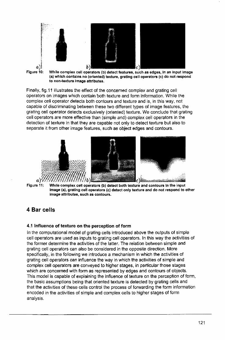
Figure While complex cell operators (b) detect features, such as edges, in an input image (a) which contains no (oriented) texture, grating cell operators (c) do not respond to non-texture image attributes.

Finally, fig.11 illustrates the effect of the concerned complex and grating cell operators on images which contain both texture and form information. While the complex cell operator detects both contours and texture and is, in this way, not capable of discriminating between these two different types of image features, the grating cell operator detects exclusively (oriented) texture. We conclude that grating cell operators are more effective than (simple and) complex cell operators in the detection of texture in that they are capable not only to detect texture but also to separate it from other image features, such as object edges and contours.

a) Figure 11: While complex cell operators (b) detect both texture and contours in the input

image (a), grating cell operators (c) detect only texture and do not respond to other image attributes, such as contours.

4 Bar cells

4.1 Influence of texture on the perception of form

In the computational model of grating cells introduced above the outputs of simple cell operators are used as inputs to grating cell operators. In this way the activities of the former determine the activities of the latter. The relation between simple and grating cell operators can also be considered in the opposite direction. More specifically, in the following we introduce a mechanism in which the activities of grating cell operators can influence the way in which the activities of simple and complex cell operators are conveyed to higher stages, in particular those stages which are concerned with form as represented by edges and contours of objects. This model is capable of explaining the influence of texture on the perception of form, the basic assumptions being that oriented texture is detected by grating cells and that the activities of these cells control the process of forwarding the form information encoded in the activities of simple and complex cells to higher stages of form analysis.

121

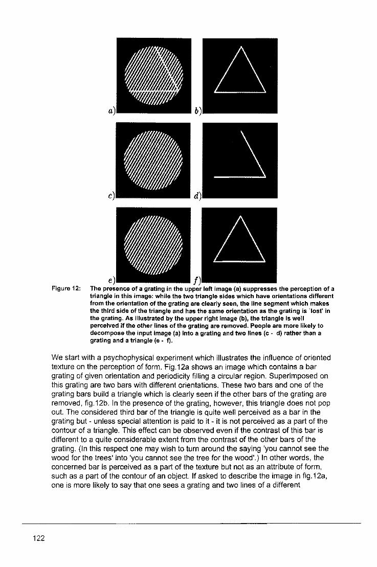
122

a) b)

c)

e) Figure 12: The presence of a grating in the upper left image (a) suppresses the perception of a

triangle in this image: while the two triangle sides which have orientations different from the orientation of the grating are clearly seen, the line segment which makes the third side of the triangle and has the same orientation as the grating is 'lost' in the grating. As illustrated by the upper right Image (b), the triangle is well perceived if the other lines of the grating are removed. People are more likely to decompose the Input image (a) into a grating and two lines (c· d) rather than a grating and a triangle (e· f).

We start with a psychophysical experiment which illustrates the influence of oriented texture on the perception of form. Fig.12a shows an image which contains a bar grating of given orientation and periodicity filling a circular region. Superimposed on this grating are two bars with different orientations. These two bars and one of the grating bars build a triangle which is clearly seen if the other bars of the grating are removed, fig.12b. In the presence of the grating, however, this triangle does not pop out. The considered third bar of the triangle is quite well perceived as a bar in the grating but - unless special attention is paid to it - it is not perceived as a part of the contour of a triangle. This effect can be observed even if the contrast of this bar is different to a quite considerable extent from the contrast of the other bars of the grating. (In this respect one may wish to turn around the saying 'you cannot see the wood for the trees' into 'you cannot see the tree for the wood'.) In other words, the concerned bar is perceived as a part of the texture but not as an attribute of form, such as a part of the contour of an object. If asked to describe the image in fig.12a, one is more likely to say that one sees a grating and two lines of a different

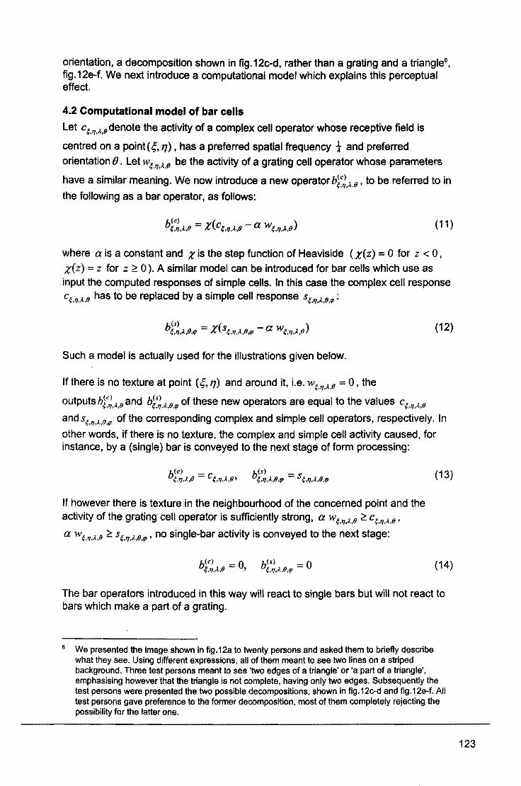
orientation, a decomposition shown in fig. 12c·d, rather than a grating and a triangle6,

fig. 12e-f. We next introduce a computational model which explains this perceptual effect.

4.2 Computational model of bar cells

Let c':,1/.A,8denote the activity of a complex cell operator whose receptive field is

centred on a point (~, TJ) , has a preferred spatial frequency t and preferred orientation 8. Let w,:.1/.A.8 be the activity of a grating cell operator whose parameters

have a similar meaning. We now introduce a new operator bt~.A,8 ' to be referred to in the following as a bar operator, as follows:

b(C) = v( C - a W ) :.1/.A,8 Jt, :.1/,A,8 ':,1/,A,e (11 )

where a is a constant and X is the step function of Heaviside (X(z) = 0 for z < 0, X(z) = z for z ~ 0). A similar model can be introduced for bar cells which use as input the computed responses of simple cells. In this case the complex cell response C q,1/,A.8 has to be replaced by a simple cell response S :,71.A,e,'P :

b(S) =X(s -aw ) :,T/.A,e,'P ':.1/,A,8,f/J :,71,A,O (12)

Such a model is actually used for the illustrations given below.

If there is no texture at point (~, q) and around it, i.e. W:,1].A.O = 0, the

outputs bt~.J..o and bg~.J.,o'f/J of these new operators are equal to the values C ':,1/,A,O

ands:.T/,;',O,f/J of the corresponding complex and simple cell operators, respectively, In

other words, if there is no texture, the complex and simple cell activity caused, for instance, by a (single) bar is conveyed to the next stage of form processing:

If however there is texture in the neighbourhood of the concerned point and the activity of the grating cell operator is sufficiently strong, a w':,T/,;',e ~ c:.1].;.,o'

a w:.T/,J.,o ~ S:,T/,A,O.f/J' no single-bar activity is conveyed to the next stage:

b~C.1]). ',0 = 0, b~s) '0 = 0 ~ '" ~,rJ." •• 1{)

(13)

(14)

The bar operators introduced in this way will react to single bars but will not react to bars which make a part of a grating.

6 We presented the image shown in fig.12a to twenty persons and asked them to briefly describe what they see. Using different expressions. all of them meant to see two lines on a striped background. Three test persons meant to see 'two edges of a triangle' or 'a part of a triangle', emphasising however that the triangle is not complete, having only two edges. Subsequently the test persons were presented the two possible decompositions, shown in fig.12c-d and fig.12e-f. All test persons gave preference to the former decomposition, most of them completely rejecting the possibility for the latter one.

123

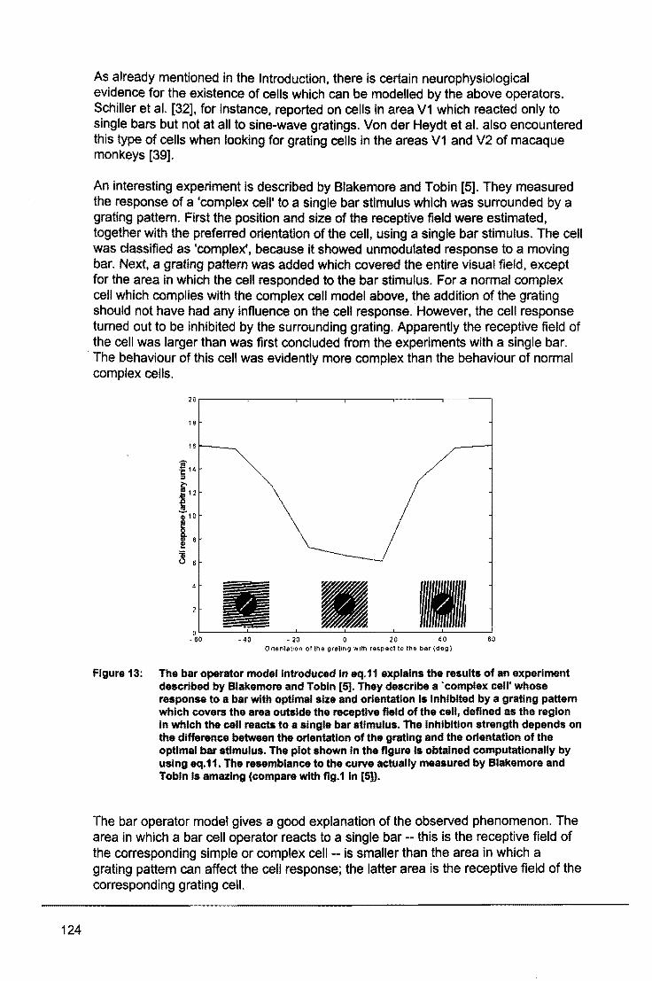
124

As already mentioned in the Introduction, there is certain neurophysiological evidence for the existence of cells which can be modelled by the above operators. Schiller et al. [32], for instance, reported on cells in area V1 which reacted only to single bars but not at all to sine-wave gratings. Von der Heydt et al. also encountered this type of cells when looking for grating cells in the areas V1 and V2 of macaque monkeys [39].

An interesting experiment is described by Blakemore and Tobin [5]. They measured the response of a 'complex cell' to a single bar stimulus which was surrounded by a grating pattern. First the position and size of the receptive field were estimated, together with the preferred orientation of the cell, using a single bar stimulus. The cell was classified as 'complex', because it showed unmodulated response to a moving bar. Next, a grating pattern was added which covered the entire visual field, except for the area in which the cell responded to the bar stimulus. For a normal complex cell which complies with the complex cell model above, the addition of the grating should not have had any influence on the cell response. However, the cell response turned out to be inhibited by the surrounding grating. Apparently the receptive field of the cell was larger than was first concluded from the experiments with a single bar. The behaviour of this cell was evidently more complex than the behaviour of normal complex cells.

20,-----,-----,-----,-----,-----~----~

18

16r---_

o~----~----~----~----J-----~----~ - 60 ·40 -20 0 20 40 60

Ooeol&llon of the grating Wltn respoct to tho bar (dog)

Figure 13: The bar operator model Introduced In eq.11 explains the results of an experiment described by Blakemore and Tobin [5]. They describe a 'complex cell' whose response to a bar with optimal size and orientation Is Inhibited by a grating pattern which covers the area outside the receptive field of the cell, defined as the region in which the cell reacts to a single bar stimulus. The Inhibition strength depends on the difference between the orientation of the grating and the orientation of the optimal bar stimulus. The plot shown in the figure Is obtained computationally by using eq.11. The resemblance to the curve actually measured by Blakemore and Tobin is amazing (compare with flg.1 in [5]).

The bar operator model gives a good explanation of the observed phenomenon. The area in which a bar cell operator reacts to a single bar -- this is the receptive field of the corresponding simple or complex cell .- is smaller than the area in which a grating pattem can affect the cell response; the latter area is the receptive field of the corresponding grating cell.

Fig.13 shows the computed response of a bar cell operator to a stimulus that consists of a bar with optimal orientation and size and a grating pattern that surrounds the receptive field of the corresponding simple cell. The inhibition of the cell response is strongest when the orientation of the grating coincides with the orientation of the optimal bar stimulus. In the experiment of Blakemore and Tobin, the response of the cell was reduced to the level of spontaneous discharge activity of the cell. In our computer model the response is attenuated by a factor of 2.5. When the deviation orientation difference is larger than 60°, there is no inhibition by the grating.

The bar operator model can in principle be extended by integration of the suppression term in eq.11 over a range of spatial frequencies:

(15)

In this case, the complex-cell term c~.r;,A.,8 is inhibited not only by the grating cell term

w';,r;,il,8 which corresponds to the same main spatial frequency t, but also by similar

terms w~,r;,A',8 corresponding to other spatial frequencies,. The plausibility of this

extension can be tested by measuring the response of single-bar cells of the type described by Schiller et al. [32] and Von der Heydt et al. [39] as a function of both the width of the bars and the (fundamental) frequency of the bar grating.

The computational model proposed above concerns the process of conveying or not conveying the activities of simple and complex cells to higher stages. We are deliberately not concerned with the possibility for a negative feedback from grating cells to complex and simple cells, since as demonstrated elsewhere [29] such interactions may radically change the impulse response of the computational model of simple cells and bring it in contradiction with the actually measured impulse responses of such cells.

125

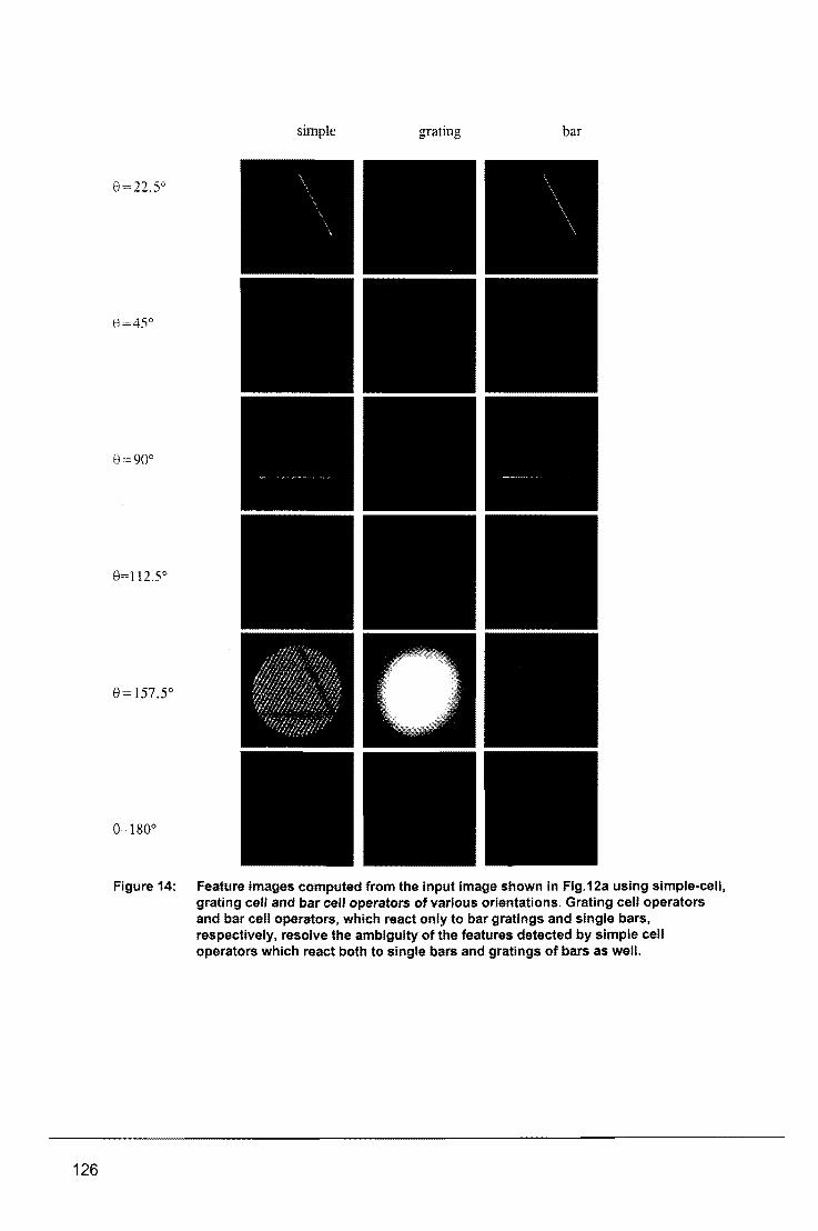
126

simple grating bar

8=22.5°

9=112.5°

e= 157.5°

Figure 14: Feature images computed from the input image shown in Fig.12a using simple-cell, grating cell and bar cell operators of various orientations. Grating cell operators and bar cell operators, which react only to bar gratings and single bars, respectively, resolve the ambiguity of the features detected by simple cell operators which react both to single bars and gratings of bars as well.

4.3 Biological role - selective detection of bars, lines and contours

Fig.14 shows a set of feature images computed with various operators from the input image shown in fig.12a. The images in the first column of fig.14 are obtained by applying simple-cell operators7 of various orientations and the same preferred spatial frequency as the fundamental spatial frequency of the grating in the input image. The second column of fig.14 shows the feature images computed with the corresponding grating cell operators and the third column shows the feature images computed with the bar operators according to the model introduced in eq.12 above. While the simple cell operators detect aU white bars, independently whether they are isolated or make part of a periodic pattern, grating cell and bar operators are more selective, in that the former react only to periodic bar patterns and the latter only to bars which do not make part of a periodic structure. Fig.15 shows the superpositions of the images in each of the three columns of fig.14. The superpositions of grating and bar operators shown in fig.15c and fig.15d, respectively, can be generated also if these operators are applied to the images shown in fig.12c and fig.12d, respectively. In this way, the result of the application of grating and bar cell operators corresponds to the perceptually plausible decomposition of the input image into texture and form information (fig. 12c-d).

A similar image as the one shown in fig.15a is an illusion taken from [18], fig. 16a, in which a part of a rectangular contour line is occluded by a grating pattern. While simple cell operators (fig.16b) show an ambiguous response with respect to form and texture, the grating and bar cell operators are able to resolve this ambiguity, fig. 16c-d.

a) Figure 15: Feature images computed as superpositions of feature images obtained with

simple (b), grating (c) and bar (d) cell operators for different orientations. The ambiguity of simple cell responses for gratings and single bars is resolved by grating and bar cell operators. As to the image shown in c), the actual grating cell feature image has been replaced by an image in which the region of activity of grating cells with given preferred orientation and periodicity is filled in with the optimal grating stimulus.

The results of a computer simulation experiment with a natural image is shown in fig.17. The input image (a) shows a bottle standing on a table with a striped tablecloth. It was already shown that grating cell operators, in contrast to simple and complex cells operators, are able to detect the texture areas in the image, while they do not react to the contours of the bottle. The bar cell operator is complementary to the grating cell operator in that it reacts only to the contours of the bottle and not to texture. The combination of grating and bar cell operators gives visual information segregation which corresponds to the segregation inferred from psychophysical experiments.

7 More precisely, symmetrical 'centre-on' operators (cp = 0) are used.

127

128

a) Figure 16:

c) d) Another example of a grating pattern suppressing a contour line (a). The example is taken from Kanizsa [181. The feature Images computed as superpositions of feature images obtained with simple cell, grating cell and bar operators are shown in (b), (c) and (d) respectively.

b Figure 17: An input Image (a) and feature images computed as superpositions of feature

images obtained with simple (b), grating (c) and bar (d) cell operators for different orientations.

5 Summary and conclusions

In this paper we introduced computational models of periodic- and aperiodic-pattern selective cells, called grating and bar cells, respectively, and applied them to different visual stimuli in order to verify the models and reveal the biological role of the concerned cells.

The computational model of grating cells employs an AND-type non-linearity used to combine the responses of simple cells with symmetric receptive field profiles and opposite polarities in such a way that a grating cell will respond strongly to a bar grating of a given orientation and periodicity but will not react to single bars. The parameters of our model are chosen in such a way that all properties of grating cells, as reported in [39]. are successfully mimicked. These properties range from orientation and spatial frequency bandwidths of such cells to their characteristic responses to selected aperiodic patterns such as isolated bars and edges, and periodic patterns such as gratings of different orientations and periodicities and checker board patterns.

As grating cell operators are selective for periodic oriented patterns, it was concluded by the neurophysiologists who discovered this type of cells that they playa certain role in the perception and processing of oriented texture at an early stage in the visual system. Since other orientation selective operators, such as simple and complex cell operators, have already been shown in computer simulations to be capable of detecting oriented texture, our main concern in this respect was that of what the added value of grating cells might be with respect to the perception and processing of texture.

Firstly, we demonstrated by means of computer simulations that grating cell operators succeed to detect oriented texture where simple and complex cell operators do so. Both types of operators give comparable results for segmentation of different texture regions, too. Then we illustrated the difference between simple and complex cell operators, on one hand, and grating cell operators, on the other hand, by computer simulations in which the two types of operators are applied to input images which contain contours but do not contain texture. In such cases simple and complex cell operators will give the wrong results if used as texture detecting operators. They respond not only to texture, but to other image features such as edges, lines and contours, as well. In contrast, grating cell operators detect no features such as isolated lines and edges. In this way grating cell operators fulfill a very important requirement imposed on texture processing operators in that, next to successfully detecting (Oriented) texture. they do not react to other image attributes such as object contours.

The difference between simple and complex cell operators, on one hand, and grating cell operators, on the other hand, is especially well illustrated when these operators are applied to images which contain both texture and form information. While

-complex cell operators, for instance, detect both contours and texture and are, in this way, not capable of discriminating between these two different types of image features, grating cell operators detect exclusively (Oriented) texture. We conclude that grating cell operators are more effective than simple and complex cell operators in the detection and processing of texture in that they are capable not only to detect texture where it is actually present and also detected by simple or complex cell operators, but also to separate it from other image features, such as edges and contours.

The computational model of a bar cell employs a thresholded difference of the activity of a complex or a simple cell and a grating cell with the same preferred orientation and spatial frequency. In the presence of oriented texture in the receptive fields of the concemed cells, in particular in the presence of a grating which regarding its orientation and periodicity is the optimal stimulus for the concemed grating cell, the strong grating cell response will have a strong inhibitory effect on the response of the bar cell and eventually suppress its response completely. If there is no texture in the receptive fields of the concemed cells there will be no inhibitory effect from the grating cell and the bar cell will simply convey the response of the concemed complex or simple cell.

This simple model is capable of qualitatively reproducing the main feature in the behaviour of bar cells to respond to single bars and decrease their responses with the addition of further bars to form a periodic pattern. Furthermore the model amazingly well reproduces the form of the response of such a cell as a function of the orientation of a grating which inhibits the response to an optimal single bar stimulus. The proposed model is also quite successful in explaining the effects of gratings on the perception of bars as these are known from psychophysical experiments.

129

130

The proposed model of bar cells is conceived in such a way that its response and the response of the related grating cell complement each other, in that their sum would produce the response of the corresponding complex or simple cell. In this way, a pair of a grating and an associated bar cell carries the same information as the corresponding complex or simple cell. The role of this new representation of visual information is likely to be related to the efficient solution of specific visual tasks, in that such a representation makes certain features of the visual information, such as the presence of oriented texture or object contours, explicit, i.e. immediately accessible for interpretation without the need for further processing. This increasing functional specialisation in the transition of simple and complex cell activities to grating and bar cell activities seems to follow the same principles of increasing functional specialisation which is followed when the representation of visual information delivered by orientationally unselective retinal ganglion and LGN cells is transformed into a representation encoded in the activities of the orientationally selective simple and complex cells.

The question about the role of the transformation of visual information from a representation by simple and complex cell activities to bar and grating cell activities

. can be accessed only from the viewpoint of the goals of natural vision information processing. While the simple and complex cell operators detect bars, independently whether these bars are isolated or make part of a periodic pattern, grating and bar cell operators are more selective, in that the former react only to periodic bar patterns and the latter only to bars which do not make part of a periodic structure. In this way the latter representation resolves the ambiguity of the former one with respect to the discrimination between important image features such as contours and texture. This representation explains the (psychophysical) observation that the perception of texture and the perception of form are complementary processes.

References

[1] Albrecht D.G., Thorell L.G., De Valois RL.: "Spatial and temporal properties of receptive fields in monkey and cat visual cortex", Abstracts 9th Meeting Soc. for Neuroscience (Atlanta, 1979) p.775.

[2] Albrecht D.G., De Valois RL., Thorell L.G.: "Visual cortical neurons: Are bars or gratings the optimal stimuli?", Science, Vol.207 (1980) pp.88-90.

[3] Andrews B.W., Pollen D.A.: "Relationship between spatial frequency selectivity and receptive field profile of simple cells", J. Physiology (London), Vol.287 (1979) pp.163-176.

[4] Bergen J.R, Landy M.S.: "Computational modelling of visual texture segregation". In Landy M.S., Movshon J.A. (eds.): Computational models of visual processing, MIT Press, Cambridge, Mass., 1991, pp.253-271.

[5] Blakemore C., Tobin E.A.: "Lateral inhibition between orientation detectors in the cat's visual cortex", Experimental Brain Research, Vol.15 (1972) pp.439-440.

[6] Burr D.C., Morrone M.C., Spinelli D.: "Evidence for edge and bar detectors in human vision", Vision Research, Vol.29 (1989) pp.419-431.

[7] Daugman J.G.: "Uncertainty relations for resolution in space, spatial frequency, and orientation optimized by two-dimensional visual cortical filters", Journal of the Optical Society of America A, Vol.2 (1985) pp.1160-1169.

{81 De Valois R.L., Albrecht D.G., Thorell L.G.: "Cortical cells: bar and edge detectors, or spatial frequency filters". In: Cool S.J., Smith III E.L. (eds.): Frontiers of Visual Science (New York: Springer Verlag, 1978).

[9] De Valois K.K., De Valois R.L., Yund E.W.: "Responses of striate cortical cells to grating and checkerboard patterns", J. Physiology (London), Vol. 291 (1979) pp.483-505.

[10] De Valois R.L., Albrecht D.G., Thorell L.G.: "Spatial frequency selectivity of cells in macaque visual cortex", Vision Research, Vol.22 (1982) pp.545-559 .

. [11] Field D.J., Nachmias J.: "Phase reversal discrimination", Vision Research, Vol. 24 (1984) pp.333-340.

[12] Field D.J., Tolhurst D.J.: "The structure and symmetry of simple cell receptive field profiles in the cat's visual cortex", Proc. Royal Soc. London, Vol. B228 (1986) pp.379-399.

[13] Glezer V.D., Tscherbach T.A., Gauselman V.E., Bondarko V.M.: "Linear and non-linear properties of simple and complex receptive fields in area 17 of the cat visual cortex", BioI. Cybern., Vol. 37 (1980) pp.195-208.

[14] Hubel D.H., Wiesel T.: "Receptive fields, binocular interaction, and functional architecture in the cat's visual cortex", J. Physiol. (London), Vol. 160 (1962), pp.106-154.

[15] Hubel D.H., Wiesel T.N.: "Sequence regularity and geometry of orientation columns in the monkey striate cortex", J. Camp. Neurol., Vol.158 (1974) pp.267 -293.

[16) Hubel D.H.: "Explorations of the primary visual cortex, 1955-1978" (1981 Nobel Prize lecture), Nature, Vol. 299 (1982) pp.515-524.

[17] Jones J.P., Palmer L.A.: "An evaluation of the two-dimensional Gabor filter model of simple receptive fields in cat striate cortex", J. Neurophysiology, Vol.58 (1987) pp. 1233-1258.

[18] Kanizsa G.: "Organization in Vision, Essays on Gestalt Perception", New York: Praeger, 1979.

[19] Kruizinga P., Petkov N.:"A computational model of Periodic-pattern-selective cells", in J. Mira and F. Sandoval (eds.), From Natural to Artificial Neural Computation, Proceedings of the Int. Workshop on Artificial Neural Networks, IWANN '95, Torremolinos (Malaga), Spain, June 7-191995, volume 930 of Lecture Notes in Computer Science, (Berlin: Springer-Verlag, 1995). pp. 90-99.

131

132

[20] Kulikowski J.J., Bishop P.O.: "Fourier analysis and spatial representation in the visual cortex", Experientia, Vol.37 (1981) pp.160-163.

[21] Macleod I.D.G., Rosenfeld A.: "The visibility of gratings: spatial frequency channels or bar-detecting units?", Vision Research, Vol. 14 (1974) pp.909-915.

[22] Maffei L., Morrone C., Pirchio M., Sandini G.: Responses of visual cortical cells to periodic and non-periodic stimuli", J. Physiology (London), Vol.296 (1979) pp.27-47.

[23] Malik J., Perona P.: "Preattentive texture discrimination with early vision mechanisms", Journal of the Optical Society A, Vol.7, No.5, 1990, pp.923-932.

[24] Manjunath B.S., Cheliappa, R.: "A unified approach to boundary perception: edges, textures, and illusory contours", IEEE Transactions on neural networks, Vol. 4, No.1, 1993, pp.96-107,

-[25] Marcelja S.: "Mathematical description of the responses of simple cortical cells", Journal of the Opt.Soc. of America, Vol. 70 (1980) pp.1297-1300.

[26] Morrone M.C., Burr D.C.: "Feature detection in human vision: Aphase­dependent energy model", Proc. of the Royal Sosciety of London, Series B, Vol.235 (1988) pp.221-245.

[27] Movshon J.A., Thompson I.D., Tolhurst D.J.: "Spatial summation in the receptive fields of simple cells in the cat's striate cortex", J. Physiology (London), Vol. 283 (1978) pp.53-77.

[28] Movshon J.A., Thompson I.D., Tolhurst D.J.: "Receptive field organisation of complex cells in the cat's striate cortex", J. Physiology (London), Vol.283 (1978) pp.79-99.

[29] Petkov N., Kruizinga P., Lourens T.: "Orientation competition in cortical ,Iters -An application to face recognition", Computing Science in The Netherlands 1993, Nov. 9-10,1993, Utrecht (Stichting Mathematisch Centrum: Amsterdam, 1993) pp.285-296.

[30] Petkov N.: "Biologically motivated computationally intensive approaches to image pattern recognition", Future Generation Computer Systems, Vol.11 (1995) pp.451-465.

[31] Pollen D., Ronner S.: "Phase relationships between adjacent simple cells in the visual cortex", Science, Vol. 212 (1981) pp.1409-1411.

[32] Schiller P.H., Finlay B.L., Volman S.F.: "Quantitative studies of single-cell properties in monkey striate cortex. III. Spatial frequencies", J. Neurophysiology, Vol.39 (1976) pp.1334-1351.

[33] Shapley R., Caelli T., Morgan M., Rentschler I.: "Computational theories of visual perception". In Spillmann L. and Wemer J.S. (eds.): Visual Perception:

The Neurophysiological Foundations (New York: Academic Press, 1990) pp.417 -448.

[34] Spitzer H. t Hochstein S.: "A complex cell receptive field model", J. Neurophysiology, Vol. 53 (1985) pp.1266-1286.

[35] Szulborski R.G., Palmer L.A.: "The two-dimensional spatial structure of non­linear subunits in the receptive fields of complex cells", Vision Research, Vol.30 (1990) pp.249-254.

[36] Tyler C.W.: "Selectivity for spatial frequency and bar width in cat visual cortex", Vision Research, Vol.18 {1978} pp.121-122.

[37] von der Heydt R.: "Approaches to visual cortical function", Rev. Physiol. Biochem. Pharmacol., Vol.108 (1987) pp.69-150.

[38] von der Heydt R., Peterhans E., DOrsteler M.R.: "Grating cells in monkey visual cortex: Coding texture". In Blum B. (ed.): Channels in the Visual Nervous System: Neurophysiology, Psychophysics and Models (Freund Publ. House Ltd.: London, 1991) pp.53-73.

[39] von der Heydt R., Peterhans E., DOrsteler M.R.: "Periodic-pattem-selective cells in monkey visual cortex", J. Neuroscience, Vol. 12 (1992) pp.1416-1434.

133

IEEE Student Branch Eindhoven

The Institute of Electrical and Electronics Engineers. Inc. is de grootste professionele organisatie van en voor elektrotechnische ingenieurs met ruim 300.000 led en in 150 landen. Onder deze leden bevinden zich ook veel studenten. Deze zijn bij IEEE verbonden door middel van Student Branches. Om de studenten voor te bereiden en kennis te laten maken met de verschillende facetten van de elektrotechniek heeft IEEE op bijna iedere technische universiteit een Student Branch opgericht.

IEEE Student Branch Eindhoven organiseert ieder jaar een symposium, een studiereis naar het buitenland en excursies naar verschillende bedrijven (in binnenw en buitenland). Met deze activiteiten hoopt de Student Branch het contact tussen toekomstige ingenieurs met de reeds in het bedrijfsleven actieve ingenieurs te onderhouden en te verbeteren.

Faculteit Wiskunde & Informatica

De faculteit Wiskunde en Informatica van de TUE verzorgt twee eerste- en twee tweedewfase opleidingen op de gebieden Technische Wiskunde en Technische Informatica. Het onderzoek van de faculteit is breed en loopt uiteen van grootschalig rekenen en cryptografie tot software voor embedded real-time systemen en 3-D computeranimatie. Op het gebied van neurale netwerken wordt zowel onderwijs gegeven (niet aileen voor de eigen faculteit) als onderzoek gedaan. De faculteit verricht veel onderzoek voor het bedrijfsleven en een belangrijk percentage van de afstudeerprojecten en aile eindprojecten van de ontwerpersopleiding zijn extern.

Rekencentrum

Het Rekencentrum heeft een groep die zich bezighoudt met applicaties ter ondersteuning van Onderwijs en Onderzoek. Er is een subgroep gericht op Statistische Programmatuur en Methodologie. Deze subgroep verzorgt diverse cursussen voor de interne en externe markt en doet ook veel consultatie. Neurale netwerken worden in deze context beschouwd als een alternatief voor sommige statistische methoden.

135

Dankwoord

De symposiumcommissie dankt de volgende personen voor hun inzet, hulp en medewerking om dit symposium tot stand te brengen:

Prof.dr. M. Rem, Rector Magnificus, TUE Prof.dr.ir. J. Vandewalle, Faculteit Toegepaste Wetenschappen, KU Leuven Dr. H.J. Kappen, Stichting Neurale Netwerken, KUN Ir. J. van Dommelen, SAS Institute B. V. Dr';r. AJ. Annema, Philips NatLab Dr. ir. MA Kraaijveld, Shelllntemational Exploration and Production B. V. Drs. D.J.N. Egberts, Biologica Ir. PP. Meiler, TNO-FEL Dr. AP. de Weijer, AKZO Nobel Central Research Ing. H. Brockmeyer, Smit Transformatoren Ir. R.M.L. Frenken, KEMA

. Prof. dr. N. Petkov, Centre for High Performance Computing, Instituut voor Wiskunde en Informatica, RUG Prof.dr.ir. W.MG. van Bokhoven, decaan Faculteit Elektrotechniek Prof. dr. P.AJ. Hi/bers, Faculteit Wiskunde en Informatica P.J.H.M Peels (ontwerp brochure)

Verder bedanken wij:

De Faculteit Elektrotechniek, IEEE Region 8, IEEE Section Benelux, het comite van aanbeveling. het bestuur van IEEE SBE, medewerkers van het congresburo aan de rUE en verder iedereen die direct of indirect een positieve bijdrage heeft geleverd aan dit symposium.

137

Comite van aanbeveling

Dr. Ir. M.J. Bastiaans Counselor IEEE-SBE

Prof. Dr. Ir. W.M.G. van Bokhoven Dekaan faculteit Elektrotechniek TUE

C. Boonstra President Philips Electronics N.V.

Prof. Dr. Ir. P.P.J. v.d. Bosch Voorzitter vakgroep Meet- en Besturingssystemen TUE

Dr. Ir. A.A.H. Damen Universitair hoofddocent vakgroep Meet- en Besturingssystemen TUE

Prof. Dr. C.C.A.M. Gielen Directeur Stichting Neurale Netwerken

Prof. Dr. M. Rem Rector magnificus Technische Universiteit Eindhoven

Prof. Dr. Ir. L. Spaanenburg Directeur Vereniging Artificiele Neurale Netwerken

Ir. A.P. Verljjsdonk Voormalig Counselor IEEE-SBE Erelid IEEE-SBE

139

Hoofdsponsor

Netwerk

Subsponsors

Shell

Honeywell

Lijst van sponsors

Universiteitsfonds Eindhoven

Faculteit Elektrotechniek, TUE

SAS Institute

Biologica

Stichting Professor Gelissenfonds

Scientific Software Benelux

Sentient Machine Research

IEEE Region 8

Vakgroep TIE, Faculteit elektrotechniek TUE

Vakgroep SES, Faculteit elektrotechniek TUE

141

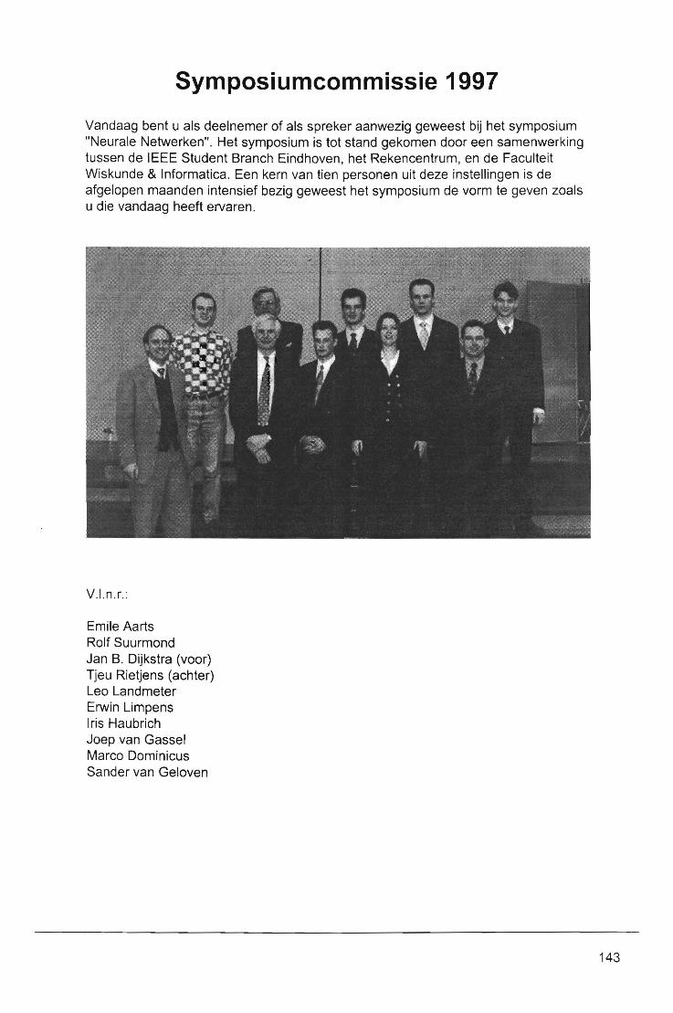
Symposiumcommissie 1997

Vandaag bent u als deelnemer of als spreker aanwezig geweest bij het symposium "Neurale Netwerken". Het symposium is tot stand gekomen door een samenwerking tussen de IEEE Student Branch Eindhoven, het Rekencentrum, en de Faculteit Wiskunde & Informatica. Een kern van tien personen uit deze insteliingen is de afgelopen maanden intensief bezig geweest het symposium de vorm te geven zoals u die vandaag heeft ervaren.

V.l.n.r.:

Emile Aarts Rolf Suurmond Jan B. Dijkstra (voor) Tjeu Rietjens (achter) Leo Landmeter Erwin Limpens Iris Haubrich Joep van Gassel Marco Dominicus Sander van Geloven

143

Proceedings behorende bij het symposium "Neurale Netwerken", gehouden op 3 april 1997 in de "De blauwe zaal" en "Promotiezaal 5" in het Auditorium van de Technische Universiteit Eindhoven.

Copyright 1997 IEEE Student Branch Eindhoven

Uitgever:

Redactie: Lay-out: Ontwerp omslag: Druk:

IEEE Student Branch Eindhoven Technische Universiteit Eindhoven Postbus 513 5600 MB Eindhoven Telefoon 040 - 247 34 33 Email ieeesb@ele.tue.nl

Symco'97 Joep van Gassel en Leo Landmeter Leo Landmeter Drukkerij De Witte

Aile rechten voorbehouden. Niets uit deze uitgave mag worden verveelvoudigd, opgeslagen in een al of niet geautomatiseerd gegevensbestand, of openbaar gemaakt, in enige vorm of op enige wijze, hetzij elektronisch, mechanisch, door fotokopien, opnamen of op enige andere manier, zonder voorafgaande schrifteljjke toestemming van de uitgever.

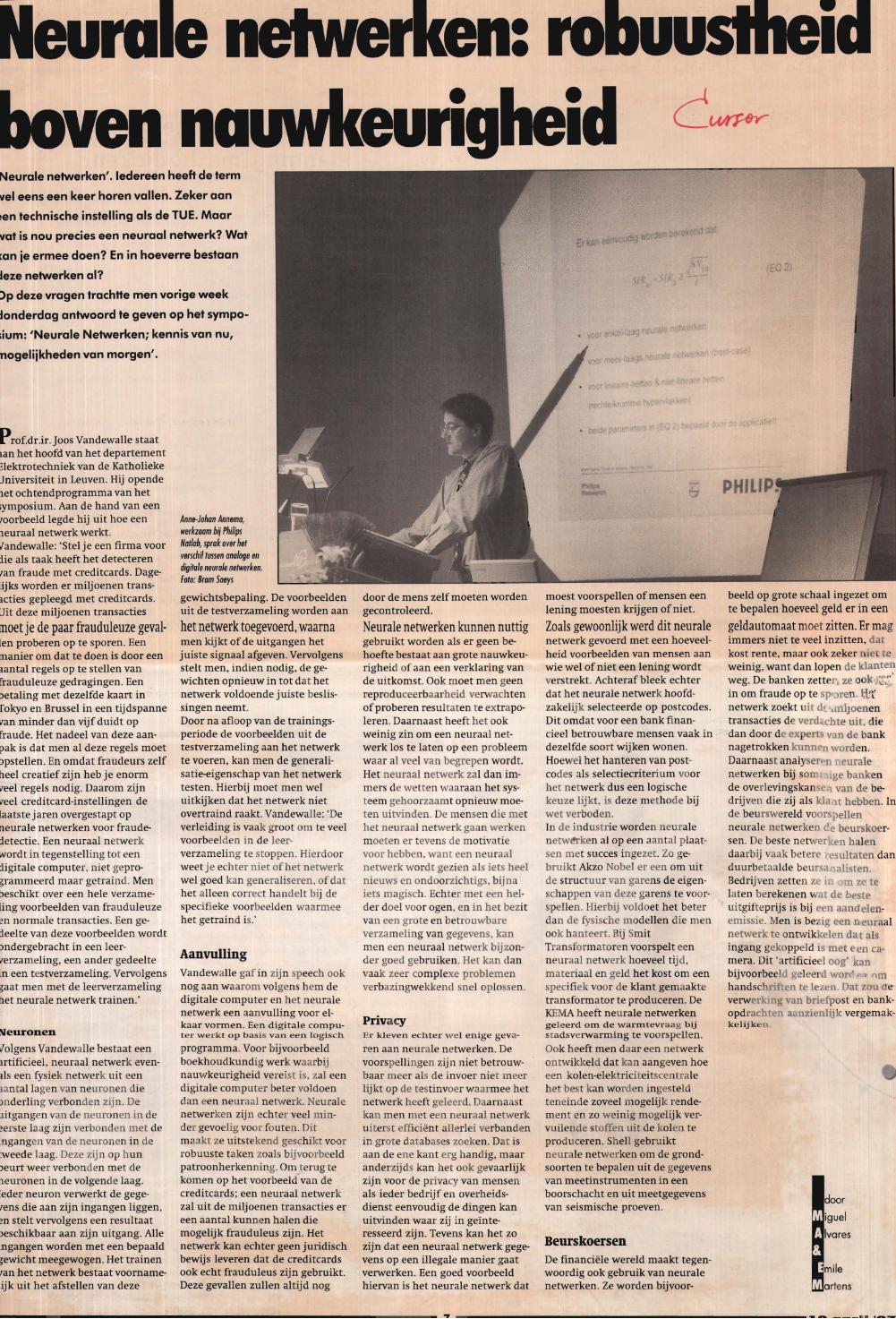
Neurale boven Neurale netwerken'. ledereen heeft de term

vel eens een keer horen vallen. Zeker aan

~en technische instelling als de TUE. Maar

vat is nou precies een neuraal netwerk? Wat

[an je ermee doen? En in hoeverre bestaan

leze netwerken al?

)p deze vragen trachtte men vorige week

londerdag antwoord te geven op het sympo­

.ium: 'Neurale Netwerken; kennis van nu,

nogelijkheden van morgen'.

P rof.dr.ir. Joos Vandewalle staat Ian het hoofd van het departement ~lektrotechniek van de Katholieke lniversiteit in Leuven. Hij opende let ochtendprogramma van het ;ymposium. Aan de hand van een roorbeeld legde hij uit hoe een leuraal netwerk werkt. vandewalle: 'Stel je een firma voor fie als taak heeft het detecteren ran fraude met creditcards. Dage­!ijks worden er miljoenen trans­lcties gepleegd met creditcards. Jit deze miljoenen transacties

moetje de paar frauduleuze geval· len proberen op te sporen. Een manier om dat te doen is door een Ian tal regels op te stellen van frauduleuze gedragingen. Een betaling met dezelfde kaart in fokyo en Brussel in een tijdspanne ~an minder dan vijf duidt op fraude. Het nadeel van deze aan­pak is dat men al deze regels moet Jpstellen. En omdat fraudeurs zelf heel creatief zijn heb je enorm veel regels nodig. Daarom zijn ~eel creditcard-instellingen de laatste jaren overgestapt op Ileurale netwerken voor fraude­jetectie. Een neuraal netwerk wordt in tegenstelling tot een jigitale computer, niet gepro­~rammeerd maar getraind. Men beschikt over een hele verzame­ling voorbeelden van frauduleuze m norma Ie transacties . Een ge­jeelte van deze voorbeelden wordt mdergebracht in een leer­verzameling, een ander gedeelte III een testverzameling. Vervolgens ~aat men met de leerverzameling het neurale netwerk trainen.'

I\leuronen

volgens Vandewalle bestaat een utificieel, neuraal netwerk even­lis een fysiek netwerk uit een lantallagen van neuronen die m derling verbonden zijn. De litgangen van de neuronen in de ~erste laag zijn verbonden met de ngangen van de neuronen in de :weede laag. Deze zij n op hun Jeurt weer verbonden met de leuronen in de volgende laag. eder neuron verwerkt de gege­rens die aan zijn ingangen liggen, ~n stelt vervolgens een resultaat Jeschikbaar aan zijn uitgang. Aile .ngangen worden met een bepaald ~ewicht meegewogen. Het trainen ran het netwerk bestaat voorname­ijk uit het afstellen van deze

Anne·lohon Annemo, werkzoom bi; Philips Notlob, sprok over hel veTSchil lussen analoge en digilole neurale nefwerken. Folo: Bram Saeys

gewichtsbepaling. De voorbeelden uit de testverzameling worden aan

het netwerk toegevoerd, waarna men kijkt of de uitgangen het juiste signaal afgeven. Vervolgens stelt men, indien nodig, de ge­wichten opnieuw in tot dat het netwerk voldoende juiste beslis­singen neemt. Door na afloop van de trainings­periode de voorbeelden uit de testverzameling aan het netwerk te voeren. kan men de generali­satie-eigenschap van het netwerk testen. Hierbij moet men weI uitkijken dat het netwerk niet overtraind raakt. Vandewalle: 'De verleiding is vaak groot om te veel voorbeelden in de leer­verzameling te stoppen. Hierdoor weet je echter niet ofhet netwerk wei goed kan generaliseren, of dat het aIleen correct handelt bij de speeifieke voorbeelden waarmee het getraind is.'

Aanvulling Vandewalle gaf in zijn speech ook nog aan waarom volgens hem de digitale computer en het neurale netwerk een aanvulling voor el­kaar vormen . Ee n digitate compu­ter werkt op basis van een logisc h

programma. Voor bijvoorbeeld boekhoudkundig werk waarbij nauwkeurigheid vereist is. zal een digitale computer beter voldoen dan een neuraal netwerk. Neurale netwerken zijn echter veel min­der gevoelig voor fouten. Dit maakt ze uitstekend geschikt voor robuuste taken zoals bijvoorbeeld patroonherkenning. Om terug te komen op het voorbeeld' van de creditcards; een neuraal netwerk zal uit de miljoenen transaeties er een aantal kunnen halen die mogelijk frauduleus zijn. Het netwerk kan echter geenjuridisch bewijs leveren dat de creditcards ook echt frauduleus zijn gebruikt. Deze gevallen zullen altijd nog

• • heid

door de mens zelf moeten worden gecontroleerd.

Neurale netwerken kunnen nuttig gebruikt worden als er geen be­hoefte bestaat aan grote nauwkeu­righeid of aan een verklaring van de uitkomst. Ook moet men geen reprod uceerbaarheid verwaeh ten of prober en resultaten te extrapo­leren. Daarnaast heeft het ook weinig zin om een neuraal net­werk los te laten op een probleem waar al veel van begrepen wordt. Het neuraal netwerk zal dan im· mers de wetten waaraan het sys­teem gehoorzaamt opnieuw moe­ten u itvinden. De mensen die met het neuraal netwerk gaan werken moeten er tevens de motivatie voor hebben. want een neuraal netwerk wordt gezien als iets heel n ieuws en ondoorzichtigs. bij na iets magisch. Echter met een he!­der doe! voor ogen. en in het bezit van een grote en betrouwbare verzameling van gegevens. kan men een neuraal netwerk bijzon­der goed gebruiken. Het kan dan vaak zeer complexe problemen verbazingwekkend snel oplossen.

Privacy Er kleven echter wei enige geva­

ren aan neurale netwerken. De voorspellingen zijn niet betrouw­baar meer als de invoer niet meer lijkt op de testinvoer waarmee het netwerk heeft geleerd. Daarnaast kan men met een neuraal netwerk u iterst efficient allerlei verbanden in grote databases zoeken. Oat is aan de ene kant erg handig. maar anderzijds kan het ook gevaarlijk zijn voor de privacy van mens en als ieder bedrijf en overheids­dienst eenvoudig de dingen kan uitvinden waar zij in geinte­resseerd zijn. Tevens kan het zo zijn dat een neuraal netwerk gege­yens op een illegale manier gaat verwerken. Een goed voorbeeld hiervan is het neurale netwerk dat

moest voorspellen of mensen een lening moesten krijgen of niet.

Zoals gewoonlijk werd dit neurale netwerk gevoerd met een hoeveel­heid voorbeelden van mensen aan wie wei of niet een lening wordt verstrekt. Achteraf bleek echter dat het neurale netwerk hoofd­zakelijk selecteerde op postcodes. Dit omdat voor een bank finan­eieel betrouwbare mensen vaak in dezelfde soort wijken wonen. Hoewel het hanteren van post­codes als selectiecriterium voor het netwerk dus een logisehe keuze lijkt . is deze methode bij wet verboden. In de industrie worden neurale netwt!rken al op een aan tal plaat­sen met succes ingezet. Zo ge­bruikt Akzo Nobel er een om uit de structuur van garens de eigen­schappen van deze garens te voor­speUen. Hierbij voldoet het beter dan de fysisehe modellen die men ook hanteert. Bij Smit Transformatoren voorspelt een neuraal netwerk hoeveel tijd. materiaal en geld het kost om een specifiek voor de klant gemaakte transformator te produceren. De KEMA heeft neurale netwerken geleerd om de warmtevraag bij stadsverwarming te voorspellen. Ook heeft men daar een netwerk ontwikkeld dat kan aangeven hoe een kolen-elektrici teitscen trale het best kan worden ingesteld teneinde zoveel mogelij k rende­ment en zo weinig mogelijk ver­vuilende stoffen uit de kolen te produceren. Shell gebruikt neurale netwerken om de grond­soorten te bepalen uit de gegevens van meetinstrumenten in een boorschaeht en uit meetgegevens van seismische proeven.

Beurskoersen De finaneiele wereld maakt tegen­woordig ook gebruik van neurale netwerken. Ze worden bijvoor-

beeld op grote schaal ingezet om te bepalen hoeveel geld er in een

geldautomaat moet zitten. Er mag immers niet te veel inzitten, dat kost rente, maar ook zeker niet te weinig. want dan lopen de klan ten weg. De banken zetter, ze ook ;J:~' in om fraude op te spl ::>ren . l:l"~

netwerk zoekt u it de ,1nljoenen transacties de verd;.chte uit. die dan door de experts van de bank nagetrokken kunnen worden. Daarnaast analyser"n neurale netwerken bij som 1ge banken de overlevingskanse.1. van de be­drijven die zij als kla 1.t hebben. In de beurswereld voorspellen neurale netwerken Ce beurskoer­sen. De beste netwerken halen daarbij vaak betere i'esultaten dan duurbetaalde beursa alisten . Bedrijven zetten ze 111 m ze te laten berekenen wat de beste uitgifteprijs is bij een aandelen­emissie. Men is bezig een neuraal netwerk te ontwikkelen da t als ingang gekoppeld is met e en ca­mera. Dit 'artificieel oog' kan bijvoorbeeld geleerd worc." f)m handschriften te lezen. Oat zou Q'e verwerlung van briefpost en bank­opdrachten aanzienlijk vergemak­kelijke n.

door

iguel

I Ivores

mile

orlens

.... - ----------------------------- - --_ ... _-