NEURAL: quantitative features for newborn EEG using Matlab

John M. O’ Toolea,∗, Geraldine B. Boylana

aNeonatal Brain Research Group, Irish Centre for Fetal and Neonatal Translational Research (INFANT), University CollegeCork, Ireland

Abstract

Background : For newborn infants in critical care, continuous monitoring of brain function can help identifyinfants at-risk of brain injury. Quantitative features allow a consistent and reproducible approach to EEGanalysis, but only when all implementation aspects are clearly defined. Methods: We detail quantitativefeatures frequently used in neonatal EEG analysis and present a Matlab software package together withexact implementation details for all features. The feature set includes stationary features that captureamplitude and frequency characteristics and features of inter-hemispheric connectivity. The software, aNeonatal Eeg featURe set in mAtLab (NEURAL), is open source and freely available. The software alsoincludes a pre-processing stage with a basic artefact removal procedure. Conclusions: NEURAL providesa common platform for quantitative analysis of neonatal EEG. This will support reproducible research andenable comparisons across independent studies. These features present summary measures of the EEG thatcan also be used in automated methods to determine brain development and health of the newborn in criticalcare.

Keywords: neonate, preterm infant, electroencephalogram, quantitative analysis, feature extraction,spectral analysis, inter-burst interval

Abbreviations: EEG, electroencephalogram; NEURAL, neonatal EEG feature set in Matlab; NICU,neonatal intensive care unit; aEEG, amplitude-integrated EEG; rEEG, range EEG; PSD, power spectraldensity; BSI, brain symmetry index; FIR, finite impulse response; IIR, infinite impulse response; DFT,discrete Fourier transform; CC, correlation coefficient.

1. Introduction

Electroencephalography (EEG) is used in the neonatal intensive care environment to monitor brainfunction of critically-ill newborns. This non-invasive and portable technology provides continuous assessmentof cortical function at the cot side, with little interruption to standard clinical care. Specialists are requiredto visually interpret the EEG to evaluate brain health, by identifying seizures if present [1], assessing brainmaturation [2], or grading brain injury [3]. Yet in many neonatal intensive care units (NICUs), provisionfor continuous reporting on the EEG of multiple infants is constrained by the availability of the specialist.Addressing this limitation, many NICUs use an amplitude-integrated EEG (aEEG) device instead of theEEG. The aEEG presents a band-pass filtered and time-compressed version of 1 or 2 channels of EEG[4, 5]. Because of the time-compression, a long duration EEG (approximately 6 hours) is summarised in 1page, making reviewing an easier task that is often preformed by non-EEG specialists, such as the treatingclinician. Yet the time-compression destroys much of the detail of the EEG waveform and many importantclinical features, such as short-duration seizures, are not presented on the aEEG [4]. In addition, artefactscan falsely enhance baseline activity or may be misinterpreted as seizures [6–8].

∗Corresponding authorEmail addresses: jotoole@ucc.ie (John M. O’ Toole), G.Boylan@ucc.ie (Geraldine B. Boylan)

Preprint submitted to Elsevier April 20, 2017

arX

iv:1

704.

0569

4v1

[ph

ysic

s.m

ed-p

h] 1

9 A

pr 2

017

Quantitative EEG analysis provides an alternative to visual interpretation, with specific advantages.First, quantitative analysis provides consistency without the varying degrees of inter-rate agreement associ-ated with visual interpretation [9]. Second, quantitative analysis can uncover attributes not accessible withvisual analysis alone, such as measures of connectivity [10, 11]. Third, quantitative analysis can facilitatereproducible research for clinical, scientific, and engineering studies. And last, quantitative analysis is anecessary component for developing fully automated methods of EEG analysis [12–14]. This is of particularimportance as automated analysis of the EEG addresses the need to provide continuous, around-the-clockEEG reporting in the NICU—something not possible with visual interpretation alone.

Quantitative features describe many aspects of newborn EEG, including sleep cycles [15–18], normativeranges [19–25], association with clinical outcomes [26–30], and functional maturation [14, 31–36]. Notstrictly defined, the term quantitative EEG features typically refers to basic signal processing measuresof frequency and amplitude. Most measures assume the signal is stationary and therefore rely on short-time analysis to circumvent this assumption. Although the features frequently appear in EEG literature,implementation details are often omitted which makes comparison between independent studies difficult, asdifferent implementations will generate different estimates. The goal of this paper, therefore, is to presenta clearly defined feature set with a software implementation that is both open source and freely available.We hope the availability of this feature set will enhance comparisons between different studies, supportreproducible research, and enhance quantitative analysis of neonatal EEG.

2. NEURAL: software package for Matlab

The software package NEURAL—a neonatal EEG feature set in matlab (v0.3.1)—runs within the Mat-lab environment (The MathWorks, Inc., Natick, Massachusetts, United States). Details on how to installand setup the Matlab code is described in the README.md file accompanying the package [37]. The packagecan generate multiple features on continuous, multi-channel EEG recordings. Features are defined specifi-cally for neonatal EEG, including preterm infants, but could also be applied to paediatric and adult EEG.

Features are grouped into 4 categories:

• amplitude: absolute amplitude and envelope of EEG signal, range EEG (similar to amplitude-integrated EEG); full list in Table B.1.

• spectral: spectral power (absolute and relative), spectral entropy (Wiener and Shannon), spectraldifferences, spectral edge frequency, and fractal dimension; full list in Table B.2.

• connectivity: coherence, cross-correlation, and brain symmetry index; full list in Table B.3.• inter-burst interval: summary measures based on the inter-burst interval annotation (only relevant

to preterm infants <32 weeks of gestational age); full list in Table B.4.

All features are listed in Tables B.2–B.4 and in file all_features_list.m. Parameters, for both thefeatures and pre-processing stage, are set in the neural_parameters.m file. For example, the low-pass filterand new sampling frequency are set in neural_parameters.m as

1 %% PREPROCESSING (lowpass filter and resample)

2 LP_fc =30; % low -pass filter cut -off

3 Fs_new =64; % down -sample to Fs_new (Hz)

Default values set in this file are reported throughout.Unless otherwise stated, we use infinite impulse response (IIR) filters for all band-pass filtering operations,

for both the artefact removal and feature estimation procedures. These filters are generated with a 5thorder Butterworth design and implemented using the forward–backwards approach to generate a zero-phaseresponse [38].

3. Pre-processing: Artefact Removal

If required, the raw EEG can be pre-processed and then saved as Matlab files. Pre-processing in-cludes a simple artefact removal procedure followed by low-pass filtering and downsampling. The function

2

resample_savemat.m performs the pre-processing. The artefact removal process removes major artefactsonly, such as electrode coupling or large-amplitude segments caused by movement; this process is detailedin the following and includes similar procedures to those described in [14]. If the EEG is still contaminatedby other artefacts, such as respiration and heart rate, other methods may also be needed [39]. After artefactremoval, all EEG channels are low-pass filtered (with a default frequency of 30 Hz; parameter LP_fc) usinga finite-impulse response (FIR) filter. This filter is designed using the window method with a Hamming win-dow of length 4,001 samples. The EEG is then downsampled to a lower frequency (default 64 Hz; parameterFs_new).

To enable the artefact removal process, set REMOVE_ART=1 if using function resample_savemat.m; other-wise, to turn off set REMOVE_ART=0. The process can also be implemented directly using the remove_artefacts.m function—see Section 5.1 for an example on how to use this function. The following details 5 stages of theartefact removal process. The process requires both the bipolar (set with BI_MONT) and referential montageof EEG.

The first stage is applied to the (M + 1)-channel referential montage. Each channel xm[n], for m =1, 2, . . . ,M,M + 1, is length-N .

1. Improper electrode placement:

(a) filter each channel xm[n] with 0.5–20 Hz bandpass filter;(b) generate correlate coefficient rpq between channel p and q, for p, q = 1, 2, . . . ,M , with p 6= q;

(c) average rpq over q, that is let rp = 1/(M − 1)∑M

q=1; q 6=p rpq for all p;(d) for rp < Tcc then remove channel p from further analysis (default Tcc = 0.15; parameter

ART_REF_LOW_CORR)

The next stage uses the M channel bipolar montage, with xm[n] now representing each bipolar channel.2. Electrode coupling:

(a) filter each channel xm[n] with 0.5–20 Hz bandpass filter;

(b) generate total power for the mth channel Pm = 1/N∑N−1

n=0 |xm[n]|2;(c) let l denote the index of left-hemisphere channels only, where {l} is a length-M/2 subset of {m};(d) let Tleft = median(Pl)/4(e) if Pl < Tleft, remove lth channel;(f) repeat previous 3 steps for right-hemisphere channels.

For the remaining stages process each bipolar channel x[n] separately.3. Continuous rows of zeros (on some EEG devices zeros replace EEG when testing for electrode impedance):

(a) identify segments x[n] = 0 for n = n+ 1, n+ 2, . . . , n+ L;(b) if L > Tmin dur, then remove (default Tmin dur = 1 second; parameter ART_ELEC_CHECK).

4. High-amplitude artefacts:

(a) filter x[n] with a [0.1–40] Hz bandpass filter;(b) generate the analytic associate of x[n] as z[n] = x[n] + jH{x[n]}, using the Hilbert transform H.(c) if |z[n]| > Tamp, then remove this segment (default Tamp = 1500µV , suitable for preterm infants

<32 weeks of gestation; parameter ART_HIGH_VOLT)(d) apply a collar around this segment and remove; default collar length is 10 seconds (parameter

ART_TIME_COLLAR).

5. Row of constant values or impulse-like activity (sudden jumps in amplitude):

(a) calculate the derivative of x[n] using the forward-difference approximation x′[n] = x[n+1]−x[n];(b) identify x′[n] = C for n = n+ 1, n+ 2, . . . , n+ L, where C is a constant;(c) if L > Tmin dur, then remove (default Tmin dur = 0.1 seconds; parameter ART_DIFF_MIN_TIME);(d) if |x′[n]| > Tamp diff, then remove (default Tamp diff = 200µV ; parameter ART_DIFF_VOLT).(e) apply a collar around both artefacts if present and remove; default length of collar is 0.5 seconds

(parameter ART_DIFF_TIME_COLLAR)

For artefacts identified on a single channel (preceding stages 3–5), the same segments are removed over allchannels. Identified artefacts are replaced by either zeros, linear interpolation, or cubic spline interpolation;

3

default is cubic spline interpolation, parameter FILTER_REPLACE_ARTEFACTS='cubic_interp'. For stages1–2, if channels are identified as artefacts they are then removed from further analysis.

4. Features

All features are estimated using the bipolar montage of the EEG. Many features are estimated withinfour different frequency bands of the EEG. Default values for these bands are [0.5–4; 4–7; 7–13; 13–30] Hz,recommended for infants ≥ 32 weeks, or [0.5–3; 3–8; 8–15; 15–30] Hz for preterm infants < 32 weeks ofgestation [14]. These bands are set with the FREQ_BANDS parameter and can also be set individually for thespecific feature, as we describe in the following.

4.1. Amplitude

Each EEG channel x[n] is filtered into the four frequency bands to generate xi[n] (i = 1, 2, 3, 4). Thesebands can be set with the parameter feat_params_st.amplitude.freq_bands. Amplitude is quantified bysignal power and signal envelope. Signal power (Ai

power) is calculated as the mean value, over time (n), of

|xi[n]|2 and amplitude of signal envelope (Eimean) is calculated as the mean value of envelope ei[n], with

ei[n] = |xi[n] + jH{xi[n]}|2 (1)

where H represents the discrete Hilbert transform implemented according to the definition described byMarple [40].

Measures of variability of the EEG about a mean value are estimated by the standard deviation (Aisd)

of xi[n] and standard deviation of the envelope ei[n]. Skewness and kurtosis (Aisk and Ai

ks) of xi[n] arecalculated to estimate a non-Gaussian processes. Moments of the probability distribution (mean, standarddeviation, skew, and kurtosis) are defined in Appendix A.

Also included are features of the range-EEG (rEEG) [33]. rEEG was proposed as an alternative toamplitude-integrated EEG (aEEG) as there is no clear definition of aEEG in the literature and most EEGmachines implement different versions of the aEEG algorithm [41]. Although another measure of amplitude,the rEEG estimates a peak-to-peak measure of voltage and therefore differs to the previous measures.

We can calculate features of rEEG using either the full-band signal x[n] or on the individual frequencybands xi[n], which gives more flexibility than aEEG which uses a fixed pass-band of 2–15 Hz [4, 41]. (Thepassband 2–15 Hz is suboptimal for neonatal EEG analysis given the predominance of delta power inneonatal EEG.) Over a short-time windowed segment, the difference between the maximum and minimumis generated

ri[l] = max(xi[n]w[n− lK])−min(xi[n]w[n− lK]) (2)

for window w[n] (default rectangular window of length 2 seconds, parameters feat_params_st.rEEG.

window_type and feat_params_st.rEEG.L_window) and time-shift factor K (parameter feat_params_st.rEEG.overlap) related to the percentage overlap H and window length M as K = dM(1−H/100)e. Whenplotting, the rEEG is transformed to a linear–log amplitude as follows

ri[l] =

{50

log 50 log ri[l] if ri[l] > 50

ri[l] otherwise(3)

Multiple features are used to summarise ri[l]: mean (Rimean) and median (Ri

median) as measures of centraltendency; the 5th (Ri

lower) and 95th (Riupper) percentiles to represent the lower and upper margins; standard

deviation (Risd), the coefficient of variation (Ri

cv = Risd/R

imean), the difference between the upper and lower

margins (Ribw = Ri

upper −Rilower) as measures of spread, and a measure of symmetry defined as

Risymm =

(Riupper −Ri

median)− (Rimedian −Ri

lower)

Ribw

(4)

where Risymm ranges from −1 to 1 with values close to 0 indicating symmetry and values close to ±1

indicating asymmetry of the rEEG.

4

4.2. Frequency

The following measures quantify spectral characteristics. First we present 3 ways to estimate the powerspectral density (PSD) for EEG signal x[n] of length-N with sampling frequency fs Hz. These different PSDestimates are used in different features. The first PSD estimate is the periodogram V [k] using a rectangularwindow

V [k] =1

Nfs

∣∣∣∣∣N−1∑n=0

x[n]e−j2πkn/N

∣∣∣∣∣2

. (5)

The second PSD estimate is the Welch periodogram P [k]

P [k] =1

LMUfs

L−1∑l=0

∣∣∣∣∣M−1∑n=0

x[n]w[n− lK]e−j2πkn/M

∣∣∣∣∣2

(6)

where w[n] is the analysis window of length M with energy U = 1/M∑M−1

n=0 |w[n]|2; default settings applya Hamming window of length 2 seconds, set with parameters feat_params_st.spectral.window_type andfeat_params_st.spectral.L_window. The time-shift factor K is related to the percentage overlap H andwindow length M , as K = dM(1 − H/100)e. Lastly, L = b(N + K −M)/Kc is the number of segments.Default value for H is 50%, set with parameter feat_params_st.spectral.overlap. And the third PSDestimate is a variant of the Welch periodogram, defined as

Pmed[k] = medianl∈[0,L−1]

1

MUfs

∣∣∣∣∣M−1∑n=0

x[n]w[n− lK]e−j2πkn/M

∣∣∣∣∣2 (7)

This estimate, which we refer to as the robust-PSD estimate, simply replaces the averaging procedure of theWelch periodogram in (6) with the median operator to generate a more robust spectral estimate [42].

For features of absolute and relative spectral power at the ith frequency band, we use the periodogramV [k] in (5):

Siabspow =

s[k]fsN

bi∑k=ai

V [k] (8)

Sirelpow =

∑bik=ai

V [k]∑b4k=a1

V [k](9)

where [ai, bi] represents the discrete frequency range of the ith frequency band. The parameter s[k] is ascaling factor, with s[k] = 2 for k = 1, 2, . . . , dN/2e − 1 and s[k] = 1 for the DC (k = 0) and Nyquistfrequency (k = N/2, for N even only). This scaling factor is applied to conserve total power in the spectrumwhen using only the positive frequencies of V [k].

Spectral entropy measures are estimated using Wiener entropy, also known as spectral flatness, andShannon entropy:

F iwiener =

exp(

1/Li

∑bik=ai

logP [k])

1/Li

∑bik=ai

P [k](10)

F ishannon = − 1

logLi

bi∑k=ai

Pi[k] log Pi[k] (11)

where Li is the length of sequence [ai, bi] representing the range of the frequency band. The normalised

spectral density Pi[k] is calculated as Pi[k] = P [k]/∑bi

k=aiP [k]. For these two entropy features, the PSD

estimate P [k] is either the periodogram in (5), the Welch periodogram in (6), or the robust estimate in (7).

5

This option is set with the parameter feat_params_st.spectral.method as either 'periodogram', 'PSD'(the default), or 'robust-PSD'.

Spectral edge frequency is defined as the frequency fSEF that contains d% (default 95%, parameterfeat_params_st.spectral.SEF) of the spectral energy; that is, we find fSEF that satisfies the relation

d

100=

∑fSEF

k=a1P [k]∑b4

k=a1P [k]

. (12)

As for the spectral entropy measures, the PSD estimate P [k] can be either one of the 3 estimates in (5), (6),and (7), set with the parameter feat_params_st.spectral.method.

Spectral difference is measured as the difference between consecutive time-slices of the spectrogram (atime-varying spectral estimate). The spectrogram, with window w[n], is defined as

S[n, k] =

∣∣∣∣∣N−1∑m=0

x[m]w[m− n]e−j2πkm/N

∣∣∣∣∣2

(13)

and the difference is calculated as

Fspecdiff = median

{1

Li

bi∑k=ai

∣∣Si[n, k]− Si[n+ 1, k]∣∣2} (14)

where Si[n, k] is normalised to the maximum spectrogram value

Si[n, k] =S[n, k]

maxn∈[0,N−1];k∈[ai,bi]

S[n, k]. (15)

And lastly, we include fractal dimension as a spectral feature because of its relation to spectral shape[43]. We present two methods to estimate fractal dimension [43, 44]. The first method, proposed by Higuchi[43] and set with parameter feat_params_st.fd.method='higuchi', generates an estimate of curve lengthCm(q) at different scale values q,

Cm(q) =(N − 1)

b(N −m)/qcq2

b(N−m)/qc∑i=1

∣∣x[m+ iq]− x[m+ (i− 1)q]∣∣. (16)

At each scale q, Cm(q) is estimated over m = 1, 2, . . . , q and then summarised by the mean value C(q) =1/q

∑qm=1 Cm(q). For a self-similar and stationary process, C(q) ∝ q−D where D is the fractal dimension

[43]. By fitting a line to the points (log q, logC(q)) over 1 ≤ q ≤ qmax, we estimate −D as the slope ofthis line. To enforce an approximate linear sampling of log q, scale values q are set to q = 1, 2, 3, 4 forq ≤ 4 and q = b2(b+5)/4c for b = 5, 6, 7, . . . otherwise. The maximum value for q is set in parameterfeat_params_st.fd.qmax and defaults to qmax = 6.

The second method, proposed by Katz and set with parameter feat_params_st.fd.method='katz', isdefined as follows [44]:

D =log(N − 1)

log(d/l) + log(N − 1). (17)

Length l is defined as the sum of the Euclidean distance between consecutive points (n, x[n]) and (n +1, x[n+ 1]) as

l =

N−2∑n=0

√1 + (x[n+ 1]− x[n])2 (18)

Extent d is defined as the maximum (Euclidean) distance from starting point (0, x[0]) to any other point(n, x[n]) as

d = max0≤n≤N−1

√n2 + (x[n]− x[1])2 (19)

6

Note that (18) and (19) differ to the definition in the often-cited interpretation by Esteller et al. [45] whichdefines the distance measure on the 1-dimensional x[n] and not on the 2-dimensional (n, x[n]) as originallyintended [44].

4.3. ConnectivityWe implement the brain symmetry index (BSI), which measures symmetry between hemispheres, ac-

cording to the specifications in [46]. First, we estimate the PSD Pm[k] for the mth channel of the EEGxm[n], for m = 1, 2, . . . ,M . For Pm[k], we can use either the periodogram in (5), the Welch periodogram in(6), or the robust-PSD estimate in (7), by setting the parameter feat_params_st.connectivity.method

to either 'periodogram', 'PSD' (default), or 'robust-PSD'. Left-hemisphere channels are ordered fromm = 1, 2, . . . ,M/2 and right-hemisphere channels ordered for m = M/2 + 1,M/2 + 2, . . . ,M . Next, we gen-erate two PSDs as the mean PSD over all channels for each hemisphere; for example, for the left hemisphere,

Pleft[k] =1

M/2

M/2∑m=1

Pm[k]

where Pm[k] represents the PSD estimate for the mth channel. A similar process produces Pright[k] for theright channels. The symmetry measure quantifies the differences in two PSDs for the ith frequency band

CiBSI =

1

Li

bi∑k=ai

∣∣∣∣Pleft[k]− Pright[k]

Pleft[k] + Pright[k]

∣∣∣∣ (20)

where [ai, bi] is the frequency range for the ith band and Li = bi − ai.Another measure of hemisphere connectivity correlates the signal envelope ei[n] in (1) for the ith fre-

quency band between channels and across the hemispheres. Channels are grouped into pairs based on theirregional location; for example, frontal channels are paired as (F3, F4), central channels as (C3, C4), and soon. Correlation coefficients (Pearson) are calculated for the mth pair ci(m), for m = 1, 2, . . . ,M/2. Themedian is used to summarise over all pairs:

Cicorr = median[ci(m)]. (21)

A global coherence measure is another approach to quantifying connectivity between regions acrosshemispheres. Coherence is calculated between channel pairs x[n] and y[n] as

Cxy[k] =|Sxy[k]|2

Pxx[k]Pyy[k](22)

where Pxx[k] (and Pyy[k]) is the auto PSD of x[n] (and y[n]) using either the Welch periodogram in (6) orthe robust-PSD in (7). The cross-PSD for x[n] and y[n], is calculated as

Sxy[k] =1

LMUfs

L−1∑l=0

(M−1∑n=0

x[n]w[n− lK]e−j2πkn/MM−1∑n′=0

y[n′]w[n′ − lK]ej2πkn′/M

). (23)

for the cross-Welch periodogram. The equivalent cross robust-PSD version replaces the mean operation overl, that is 1/L

∑L−1l=0 , with the median operator. Both the auto and cross PSDs estimates are set using the

parameter feat_params_st.connectivity.method='PSD' (default) or feat_params_st.connectivity.

method='robust-PSD'. Here, we assume that y[n] and w[n] are real-valued functions. Three features areused to summarise the coherence function Cxy[k]:

Cicoh mean =

1

Li

bi∑k=ai

Cxy[k] (24)

Cicoh max = max

k∈[ai,bi]Cxy[k] (25)

Cicoh freq max = argmax

k∈[ai,bi]

Cxy[k] (26)

7

Similar to correlation in (21), coherence features are estimated between the mth channel pairs and thensummarised by the median value over all channel pairs.

To eliminate spurious coupling caused by inaccuracies in the coherence measure, we have implemented anull-hypothesis testing process to better estimate zero coherence [47, 48]. This approach generates a lowerthreshold by assessing the likelihood that a coherence measure represents either zero coherence (the null hy-pothesis) or non-zero coherence. An empirical probability distribution is generated from multiple uncoupledsignals and is used to represent the null hypothesis that coherence is due to chance and not significantlydifferent to zero. Here, we use the Fourier-transform shuffling method to generate these uncoupled, surrogatesignals [47, 48]. The procedure, with a slight modification, is a follows:

1. compute the surrogate signal u[n] for x[n] (of length-N) as follows:

(a) generate length-N random phase ϕ[k] from a uniform distribution in the range [−π,π]; enforceconjugate symmetry on ϕ[k] with ϕ[0] = 0 and, if N is even, ϕ[N/2] = 0;

(b) multiply the magnitude spectrum of x[n] by the random phase and Fourier transform back to thetime domain

u[n] =1

N

N−1∑k=0

|X[k]| ejϕ[k]ej2πkn/N ;

2. generate v[n] from y[n] using a similar process;

3. estimate the coherence function for u[n] and v[n]

Cuv[k] =|Suv[k]|2

Pxx[k]Pyy[k](27)

similar to (22) but using Pxx[k] and Pyy[k] from signals x[n] and y[n];

4. iterate this process Niter times to generate the matrix Cuv[k] of dimension Niter ×N ;

5. let Tlower[k] equal the 100(1 − α)th percentile of Cuv[k] for each value of k, to determine if Cxy[k] isstatistical significant for p < α;

6. generate coherence Cxy[k] between x[n] and y[n] and threshold: set Cxy[k] = 0 for Cxy[k] < Tlower[k].

Parameters Niter and α are set by feat_params_st.connectivity.coherence_surr_data (default 100) andfeat_params_st.connectivity.coherence_surr_alpha (default 0.05). To calculate coherence withoutthis zero-coherence estimation procedure, set feat_params_st.connectivity.coherence_surr_data=0.The modification of the method here, not in the original procedure [47, 48], is to use Pxx[k] instead of Puu[k]in (27). We base this on the assumption that because the magnitude spectrum for u[k] and x[k] are equal,therefore PSDs should also be equal. The whole procedure to generate the threshold Tlower[k] can be slowand this modification reduces computational time by approximately one-half.

For all connectivity measures using the PSD, the window type and overlap for the PSDs can be setusing the parameters feat_params_st.connectivity.PSD_window and feat_params_st.connectivity.

overlap.

4.4. Burst and Inter-burst Intervals

The EEG of preterm infants shows a discontinuous pattern with short-duration bursts of activity al-ternating with longer quiescent periods. As the infant maturates, the burst periods become longer andquiescent periods shorter so that eventually the EEG becomes continuous as the infant approaches termage. Discontinuous activity, which predominates in prematurity, consists of intermittent bursts against abackground pattern of low-amplitude activity known as inter-burst intervals (IBI). To quantify this burst–inter-burst pattern, a burst detection method is needed to first detect the bursts before summarising thebursting pattern. We use the burst-detection algorithm proposed by O’ Toole et al. [49]. The algorithmis freely available at https://github.com/otoolej/burst_detector and is used to generate the followingfeatures.

8

The burst detection algorithm estimates the burst annotation b[n], with b[n] = 0 for inter-bursts andb[n] = 1 for bursts. Summary measures of temporal evolution of the bursting pattern include burst percent-age, calculated as

Bburst% =100

N

N−1∑n=0

b[n] (28)

and burst number Bburst#, defined as the number of detected bursts over b[n]. Similarly, summary measuresof the inter-burst pattern includes BIBI max, the maximum duration of all IBIs, and BIBI median the medianduration of IBIs.

4.5. Short-time and multi-channel analysis

Amplitude, frequency, and connectivity features are estimated on a short-time basis: features are calcu-lated over a short duration window and this window is shifted in time; default window length is 64 secondswith an overlap of 50%, set with parameters EPOCH_LENGTH and EPOCH_OVERLAP. The median value is usedto summarise these features over all analysis windows. For the amplitude, frequency, and bursting features,the features are estimated separately on each channel. Again, the median value is used to summarise overall channels.

5. Examples

5.1. Removing artefacts

To describe how the artefact removal procedure works, we present an example with simulated EEG. Thefunction gen_test_EEGdata.m generates coloured Gaussian noise as a proxy for neonatal EEG:

1 % generates 2 minutes of EEG -like data sampled at 256 Hz:

2 Fs = 256;

3 data_st = gen_test_EEGdata (2*60,Fs ,1);

The function returns the test data as both 9-channel referential montage (data_st.eeg_data_ref) and the8-channel bipolar montage (data_st.eeg_dat). Next, we simulate a faulty recording on electrode F3:

1 N = size(data_st.eeg_data_ref ,2);

2 if3 = find(strcmp(data_st.ch_labels_ref ,'F3'));3 data_st.eeg_data_ref(if3 ,:) = randn(1,N).*10;

Then simulate an electrode coupling between C4 and Cz

1 ic4 = find(strcmp(data_st.ch_labels_ref ,'C4'));2 icz = find(strcmp(data_st.ch_labels_ref ,'Cz'));3 data_st.eeg_data_ref(icz ,:) = data_st.eeg_data_ref(ic4 ,:)+randn(1,N).*5;

and then re-generate the bipolar montage

1 [data_st.eeg_data ,data_st.ch_labels] = set_bi_montage( ...

2 data_st.eeg_data_ref ,data_st.ch_labels_ref ,data_st.ch_labels_bi);

The simulated EEG is displayed in Fig. 1 using the referential montage and in Fig. 2 using the bipolarmontage.

To detect and remove these simulated artefacts, we use the remove_artefacts.m function:

1 eeg_art = remove_artefacts(data_st.eeg_data ,data_st.ch_labels , ...

2 data_st.Fs ,data_st.eeg_data_ref ,data_st.ch_labels_ref);

which returns the data in bipolar montage with channels C4-Cz and F3-C3 replaced by NaN values to indicateartefacts. The artefact identification process, relating to steps 1 and 2 in Section 3, is illustrated in Figs. 1and 2.

9

L

R

300 µV

2 secondsCz−Ref

O1−Ref

T3−Ref

C3−Ref

F3−Ref

O2−Ref

C4−Ref

T4−Ref

F4−Ref

0 0.5 1

CC

*

Figure 1: Referential montage of simulated EEG data (coloured Gaussian noise). All channels, expect for F3, are highlycorrelated [correlation coefficient (CC) r > 0.8, right-hand side]. CCs are generated by averaging correlations between eachchannel and all other channels. Channels with CCs below the given threshold (r = 0.15, vertical dashed line) are removed(denoted with the ∗ symbol), as is the case here for F3.

0 200

power (µV 2)

*

L

R

300 µV

2 secondsC3−O1

C4−O2

Cz−C3

C4−Cz

C3−T3

C4−T4

F3−C3

F4−C4

Figure 2: Bipolar montage of EEG in Fig. 1. Total power is assessed for each channel and plotted in left-hand side figure;channel F3-C3 is not included because F3 was removed in previous process (see Fig. 1). Channels with total power less thanthreshold (determined from median values of left and right hemisphere’s separately) are denoted with ∗ and removed fromfurther analysis.

10

5.2. Calculating Features

Features are estimated using the generate_all_features function, as the following example shows.First, we generate 5 minutes of test data with a 64 Hz sampling rate:

1 data_st = gen_test_EEGdata (5*60 ,64 ,1);

Then, define the feature set as follows:

1 feature_set = {'spectral_relative_power ','connectivity_BSI ','rEEG_SD '};

Relative spectral power Sirelpow and BSI Ci

BSI are defined in equations (9) and (20), respectively; standard

deviation of rEEG Risd is defined in Section 4.1. We can also use the parameter file neural_parameters.m

to define the feature set. The full list of features are in Tables B.2– B.4. And lastly, we estimate the featuresusing generate_all_features:

1 feat_st = generate_all_features(data_st ,[], feature_set);

Features are returned as a structure, with 1 feature for each of the 4 frequency bands.

1 feat_st =

2 spectral_relative_power: [0.8672 0.0913 0.0350 0.0243]

3 connectivity_BSI: [0.0614 0.0489 0.0455 0.0505]

4 rEEG_SD: [3.1808 6.9492 4.5940 3.3538]

For the next example we calculate features of the rEEG. Simulated EEG, intended to resemble a discon-tinuous trace of preterm EEG, is generated as

1 data_st = gen_test_EEGdata(duration ,Fs ,1,1);

with duration=4*60*60 (4 hours of EEG) and Fs=64. We then band-pass filter this simulated EEG with a1–20 Hz filter by setting

1 feat_params_st.rEEG.freq_bands = [1 20];

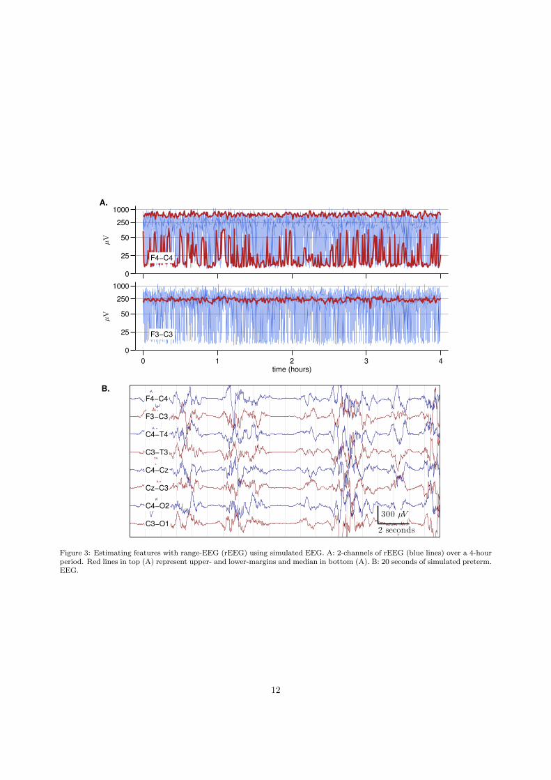
in the parameter file (neural_parameters.m). Fig. 3(B) shows a 20-second epoch of the 4-hour multichannelEEG. We can view the rEEG by plotting the second output argument from the rEEG function

1 [~,reeg_left] = rEEG(data_st.eeg_data (7,:),Fs);

2 [~, reeg_right] = rEEG(data_st.eeg_data (8,:),Fs);

where reeg_left and reeg_right represent the rEEG generated for channels F3-C3 and F4-C4. Thesesignals are plotted in Fig. 3(A). Next, assuming we want to estimate median, upper- and lower-margins ofrEEG (Rmedian, Rlower, and Rupper as defined in Section 4.1), we do as follows:

1 feats = generate_all_features(data_st ,{'F3-C3','F4 -C4'}, ...

2 {'rEEG_lower_margin ','rEEG_upper_margin ','rEEG_median '});

For the example in Fig. 3, we find median value of Rmedian = 228µV , and lower–upper margins of [15–578]µV .

11

0

25

50

250

1000

µV

F4−C4

0 1 2 3 4

0

25

50

250

1000

time (hours)

µV

F3−C3

A.

L

R

300 µV

2 secondsC3−O1

C4−O2

Cz−C3

C4−Cz

C3−T3

C4−T4

F3−C3

F4−C4

B.

Figure 3: Estimating features with range-EEG (rEEG) using simulated EEG. A: 2-channels of rEEG (blue lines) over a 4-hourperiod. Red lines in top (A) represent upper- and lower-margins and median in bottom (A). B: 20 seconds of simulated preterm.EEG.

12

6. Discussion

The presented feature set contains commonly-used features for quantitative analysis of newborn EEG.The set is implement in Matlab and freely available as open source code to use and modify as required [37].The features are clearly defined with all implementation details. Research publications often omit thesedetails yet they are essential for reproducible research and for comparing results across independent studies.For example, power in the delta frequency band will depend on a number of factors—such as filtering (ifapplied, and if so what type of filter used), power spectral density estimation (what type of estimate andwhat parameters used), and how to calculate the power (either sum over range in the frequency domain orenergy of filtered signal in the time domain). Different implementations will give different estimates of thedelta power, therefore undermining comparisons across studies. The availability of a common feature set,such as the one presented here, will enable both direct comparisons and reproducible research.

Our goal was to present quantitative features commonly used in newborn EEG [3, 14–36] and not includean exhaustive list of all possible features. For example, we restricted the set to stationary features andimplemented a short-time procedure to accommodate for the non-stationary aspects of EEG. Although non-stationary methods have been used to analyse newborn EEG [11, 50–52], we do not include these here becauseof the following: first, these nonstationary methods are often developed for specific applications, such asdetecting seizures [50]; second, their complexity limits their use, as typically a detailed-level of understandingof these methods is required before implementation [52]; and third, in many cases the assumption of short-time stationarity may be acceptable for the required application, for example in seizure detection [13]. Futureiterations could expand the scope of feature set, to include features such as more advanced connectivitymeasures [53] or methods to quantify activity cycling in preterm newborns [54].

In conclusion, the NEURAL software package provides a common platform for quantitative analysis ofmulti-channel EEG for newborn infants. The software will assist reproducible research and consistencyacross independent studies. Many of the features, with the exception of the burst and inter-burst features,may also be of use for paediatric and adult EEG. These quantitative features can also be used to developautomated methods for newborn, such as automated detection of seizures [13, 50] or estimation of brainmaturation [14].

7. Acknowledgements

This work was supported by Science Foundation Ireland (research-centre award INFANT-12/RC/2272and investigator award 15/SIRG/3580). We thank Brian Murphy for help with testing the Matlab code.

Appendix A. Moments for Stationary Random Variable

The first 4 moments (mean, standard deviation, skewness, and kurtosis) for random variable x[n] areestimated as follows: mean

x =1

N

N−1∑n=0

x[n],

standard deviation

s =

√√√√ 1

N − 1

N−1∑n=0

|x[n]− x|2,

skewness

m3 =1N

∑N−1n=0 |x[n]− x|3

s3,

and kurtosis

m4 =1N

∑N−1n=0 |x[n]− x|4

s4.

13

Appendix B. List of Features

Table B.1: Amplitude features with Matlab code name. Features are calculated for each frequency band.

name description

amplitude_total_power time-domain signal: total poweramplitude_SD time-domain signal: standard deviationamplitude_skew time-domain signal: skewnessamplitude_kurtosis time-domain signal: kurtosisamplitude_env_mean envelope: mean valueamplitude_env_SD envelope: standard deviationrEEG_mean range EEG: meanrEEG_median range EEG: medianrEEG_lower_margin range EEG: lower margin (5th percentile)rEEG_upper_margin range EEG: upper margin (95th percentile)rEEG_width range EEG: upper margin - lower marginrEEG_SD range EEG: standard deviationrEEG_CV range EEG: coefficient of variationrEEG_asymmetry range EEG: measure of skew about median

Table B.2: Spectral features with Matlab code name.

name description

spectral_power† spectral power: absolutespectral_relative_power† spectral power: relative (normalised to total spectral power)spectral_flatness† spectral entropy: Wiener (measure of spectral flatness)spectral_entropy† spectral entropy: Shannonspectral_diff† difference between consecutive short-time spectral estimatesspectral_edge_frequency spectral edge frequency: 95% of spectral power contained

between 0.5 and fc Hz (cut-off frequency)FD† fractal dimension

† feature is calculated for each frequency band.

14

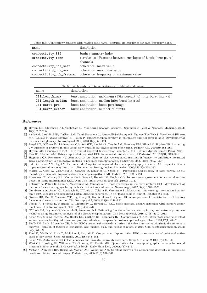
Table B.3: Connectivity features with Matlab code name. Features are calculated for each frequency band.

name description

connectivity_BSI brain symmetry indexconnectivity_corr correlation (Pearson) between envelopes of hemisphere-paired

channelsconnectivity_coh_mean coherence: mean valueconnectivity_coh_max coherence: maximum valueconnectivity_coh_freqmax coherence: frequency of maximum value

Table B.4: Inter-burst interval features with Matlab code name.

name description

IBI_length_max burst annotation: maximum (95th percentile) inter-burst intervalIBI_length_median burst annotation: median inter-burst intervalIBI_burst_prc burst annotation: burst percentageIBI_burst_number burst annotation: number of bursts

References

[1] Boylan GB, Stevenson NJ, Vanhatalo S. Monitoring neonatal seizures. Seminars in Fetal & Neonatal Medicine, 2013;18(4):202–208.

[2] Andre M, Lamblin MD, d’Allest AM, Curzi-Dascalova L, Moussalli-Salefranque F, Nguyen The Tich S, Vecchierini-BlineauMF, Wallois F, Walls-Esquivel E, Plouin P. Electroencephalography in premature and full-term infants. Developmentalfeatures and glossary. Neurophysiol Clin, 2010;40(2):59–124.

[3] Lloyd RO, O’Toole JM, Livingstone V, Hutch WD, Pavlidis E, Cronin AM, Dempsey EM, Filan PM, Boylan GB. Predicting2-y outcome in preterm infants using early multimodal physiological monitoring. Pediatr Res, 2016;80:382–388.

[4] Boylan GB. Principles of EEG. In Neonatal Cerebral Investigation, chapter 2, 9–21. Cambridge University Press, 2008.[5] Tao JD, Mathur AM. Using amplitude-integrated EEG in neonatal intensive care. J Perinatol, 2010;30(S1):S73–S81.[6] Hagmann CF, Robertson NJ, Azzopardi D. Artifacts on electroencephalograms may influence the amplitude-integrated

EEG classification: a qualitative analysis in neonatal encephalopathy. Pediatrics, 2006;118(6):2552–2554.[7] Suk D, Krauss AN, Engel M, Perlman JM. Amplitude-integrated electroencephalography in the NICU: frequent artifacts

in premature infants may limit its utility as a monitoring device. Pediatrics, 2009;123(2):e328–332.[8] Marics G, Csek A, Vasarhelyi B, Zakarias D, Schuster G, Szabo M. Prevalence and etiology of false normal aEEG

recordings in neonatal hypoxic-ischaemic encephalopathy. BMC Pediatr, 2013;13(1):194.[9] Stevenson NJ, Clancy RR, Vanhatalo S, Rosen I, Rennie JM, Boylan GB. Interobserver agreement for neonatal seizure

detection using multichannel EEG. Ann Clin Transl Neurol, 2015;2(11):1002–1011.[10] Tokariev A, Palmu K, Lano A, Metsaranta M, Vanhatalo S. Phase synchrony in the early preterm EEG: development of

methods for estimating synchrony in both oscillations and events. Neuroimage, 2012;60(2):1562–1573.[11] Omidvarnia A, Azemi G, Boashash B, O’Toole J, Colditz P, Vanhatalo S. Measuring time-varying information flow for

scalp EEG signals: orthogonalized partial directed coherence. IEEE Trans Biomed Eng, 2014;61(3):680–693.[12] Greene BR, Faul S, Marnane WP, Lightbody G, Korotchikova I, Boylan GB. A comparison of quantitative EEG features

for neonatal seizure detection. Clin Neurophysiol, 2008;119(6):1248–1261.[13] Temko A, Thomas E, Marnane W, Lightbody G, Boylan G. EEG-based neonatal seizure detection with support vector

machines. Clin Neurophysiol, 2011;122(3):464–473.[14] O’Toole JM, Boylan GB, Vanhatalo S, Stevenson NJ. Estimating functional brain maturity in very and extremely preterm

neonates using automated analysis of the electroencephalogram. Clin Neurophysiol, 2016;127(8):2910–2918.[15] Scher MS, Sun M, Steppe DA, Banks DL, Guthrie RD, Sclabassi RJ. Comparisons of EEG sleep state-specific spectral

values between healthy full-term and preterm infants at comparable postconceptional ages. Sleep, 1994;17(1):47–51.[16] Duffy FH, Als H, McAnulty GB. Infant EEG spectral coherence data during quiet sleep: unrestricted principal components

analysis—relation of factors to gestational age, medical risk, and neurobehavioral status. Clin Electroencephalogr, 2003;34(2):54–69.

[17] Paul K, Vladir K, Roth Z, Melichar J, Svojmil P. Comparison of quantitative EEG characteristics of quiet and activesleep in newborns. Sleep Medicine, 2003;4(6):543–552.

[18] Scher MS. Automated EEG-sleep analyses and neonatal neurointensive care. Sleep Medicine, 2004;5(6):533–540.[19] West CR, Harding JE, Williams CE, Gunning MI, Battin MR. Quantitative electroencephalographic patterns in normal

preterm infants over the first week after birth. Early Hum Dev, 2006;82(1):43–51.[20] Victor S, Appleton RE, Beirne M, Marson AG, Weindling AM. Spectral analysis of electroencephalography in premature

newborn infants: normal ranges. Pediatr Res, 2005;57(3):336–341.

15

[21] Pereda E, De La Cruz DM, Manas S, Garrido JM, Lopez S, Gonzalez JJ. Topography of EEG complexity in humanneonates: Effect of the postmenstrual age and the sleep state. Neurosci Lett, 2006;394(2):152–157.

[22] Okumura A, Kubota T, Tsuji T, Kato T, Hayakawa F, Watanabe K. Amplitude spectral analysis of theta/alpha/betawaves in preterm infants. Pediatr Neurol, 2006;34(1):30–34.

[23] Korotchikova I, Connolly S, Ryan CA, Murray DM, Temko A, Greene BR, Boylan GB. EEG in the healthy term newbornwithin 12 hours of birth. Clin Neurophysiol, 2009;120(6):1046–1053.

[24] Gonzalez JJ, Manas S, De Vera L, Mendez LD, Lopez S, Garrido JM, Pereda E. Assessment of electroencephalographicfunctional connectivity in term and preterm neonates. Clin Neurophysiol, 2011;122(4):696–702.

[25] Thorngate L, Foreman SW, Thomas KA. Quantification of neonatal amplitude-integrated EEG patterns. Early Hum Dev,2013;89(12):931–937.

[26] Inder TE, Buckland L, Williams CE, Spencer C, Gunning MI, Darlow BA, Volpe JJ, Gluckman PD. Lowered elec-troencephalographic spectral edge frequency predicts the presence of cerebral white matter injury in premature infants.Pediatrics, 2003;111(1):27–33.

[27] Korotchikova I, Stevenson NJ, Walsh BH, Murray DM, Boylan GB. Quantitative EEG analysis in neonatal hypoxicischaemic encephalopathy. Clin Neurophysiol, 2011;122(8):1671–1678.

[28] Williams IA, Tarullo AR, Grieve PG, Wilpers A, Vignola EF, Myers MM, Fifer WP. Fetal cerebrovascular resistance andneonatal EEG predict 18-month neurodevelopmental outcome in infants with congenital heart disease. Ultrasound ObstetGynecol, 2012;40(3):304–309.

[29] Saito M, Okumura A, Kidokoro H, Kubota T. Amplitude spectral analyses of disorganized patterns on electroencephalo-grams in preterm infants. Brain Dev, 2013;35(1):38–44.

[30] Schumacher EM, Larsson PG, Sinding-Larsen C, Aronsen R, Lindeman R, Skjeldal OH, Stiris TA. Automated spectralEEG analyses of premature infants during the first three days of life correlated with developmental outcomes at 24 months.Neonatology, 2013;103(3):205–212.

[31] Burdjalov VF, Baumgart S, Spitzer AR. Cerebral function monitoring: a new scoring system for the evaluation of brainmaturation in neonates. Pediatrics, 2003;112(4):855–861.

[32] Niemarkt HJ, Jennekens W, Pasman JW, Katgert T, Van Pul C, Gavilanes AWD, Kramer BW, Zimmermann LJ, OetomoSB, Andriessen P. Maturational changes in automated EEG spectral power analysis in preterm infants. Pediatr Res, 2011;70(5):529–534.

[33] O’Reilly D, Navakatikyan MA, Filip M, Greene D, Van Marter LJ. Peak-to-peak amplitude in neonatal brain monitoringof premature infants. Clin Neurophysiol, 2012;123(11):2139–2153.

[34] Meijer EJ, Hermans KHM, Zwanenburg A, Jennekens W, Niemarkt HJ, Cluitmans PJM, Pul CV, Wijn PFF. Functionalconnectivity in preterm infants derived from EEG coherence analysis. Eur J Paediatr Neurol, 2014;18(6):780–789.

[35] Shany E, Meledin I, Gilat S, Yogev H, Golan A, Berger I. In and ex utero maturation of premature infants electroen-cephalographic indices. Clin Neurophysiol, 2014;125(2):270–276.

[36] Saji R, Hirasawa K, Ito M, Kusuda S, Konishi Y, Taga G. Probability distributions of the electroencephalogram envelopeof preterm infants. Clin Neurophysiol, 2015;126(6):1132–1140.

[37] O’Toole JM. NEURAL: a neonatal EEG feature set in Matlab. GitHub Repository, 2016; ([online] https://github.com/otoolej/qEEG_feature_set).

[38] Oppenheim AV, Schafer RW. Discrete-Time Signal Processing. Prentice-Hall, Englewood Cliffs, NJ 07458, 1999.[39] Stevenson NJ, O’Toole JM, Korotchikova I, Boylan GB. Artefact detection in neonatal EEG. In Int. Conf. IEEE Eng.

Med. Biol. Soc. Chicago, 2014;926–929.[40] Marple Jr SL. Computing the Discrete-Time “Analytic” Signal via FFT. IEEE Trans Signal Process, 1999;47(9):2600–

2603.[41] Zhang D, Ding H. Calculation of compact amplitude-integrated EEG tracing and upper and lower margins using raw

EEG data. Health, 2013;5:885–891.[42] Zoubir AM, Koivunen V, Chakhchoukh Y, Muma M. Robust estimation in signal processing: A tutorial-style treatment

of fundamental concepts. IEEE Signal Process Mag, 2012;29(4):61–80.[43] Higuchi T. Approach to an irregular time series on the basis of the fractal theory. Phys D: Nonlinear Phenom, 1988;

31:277–283.[44] Katz MJ. Fractals and the analysis of waveforms. Comput Biol Med, 1988;18(3):145–156.[45] Esteller R, Echauz J, Tcheng T, Litt B, Pless B. Line length: an efficient feature for seizure onset detection. In Int. Conf.

IEEE Eng. Med. Biol. Soc., Istanbul, Turkey, 2001;1707–1710.[46] van Putten MJAM. The revised brain symmetry index. Clin Neurophysiol, 2007;118(11):2362–2367.[47] Prichard D, Theiler J. Generating surrogate data for time series with several simultaneously measured variables. Phys

Rev Lett, 1994;73(7):951–954.[48] Faes L, Pinna GD, Porta A, Maestri R, Nollo G. Surrogate data analysis for assessing the significance of the coherence

function. IEEE Trans Biomed Eng, 2004;51(7):1156–1166.[49] O’Toole JM, Boylan GB, Lloyd RO, Goulding RM, Vanhatalo S, Stevenson NJ. Detecting bursts in the EEG of very and

extremely premature infants using a multi-feature approach. Med Eng Phys, 2017; DOI:10.1016/j.medengphy.2017.04.003[50] Stevenson NJ, O’Toole JM, Rankine LJ, Boylan GB, Boashash B. A nonparametric feature for neonatal EEG seizure

detection based on a representation of pseudo-periodicity. Med Eng Phys, 2012;34(4):437–446.[51] Mesbah M, O’Toole JM, Colditz PB, Boashash B. Instantaneous frequency based newborn EEG seizure characterization.

EURASIP J Adv Signal Process, 2012;2012(143).[52] Boashash B, Azemi G, O’Toole JM. Time–frequency processing of nonstationary signals: advanced TFD design to aid

diagnosis with highlights from medical applications. IEEE Signal Process Mag, 2013;30(6):108–119.

16

[53] Omidvarnia A, Fransson P, Metsaranta M, Vanhatalo S. Functional bimodality in the brain networks of preterm and termhuman newborns. Cereb Cortex, 2014;24(10):2657–2668.

[54] Stevenson NJ, Palmu K, Wikstrom S, Hellstrom-Westas L, Vanhatalo S. Measuring brain activity cycling (BAC) in longterm EEG monitoring of preterm babies. Physiol Meas, 2014;35(7):1493–1508.

17