Neural Network Modelling and Multi-Objective Optimization...

i

Neural Network Modelling and Multi-Objective

Optimization of EDM Process A THESIS SUBMITTED IN PARTIAL FULFILLMENT

OF THE REQUIREMENTS FOR THE DEGREE OF

Master of Technology In

Production Engineering

By

SHIBA NARAYAN SAHU

(210ME2139)

Under the Supervision of

Prof. C.K BISWAS

Department of Mechanical Engineering

National Institute of Technology

Rourkela, Orissa

2012

ii

National Institute of Technology

Rourkela

CERTIFICATE

This is to certify that thesis entitled, “NEURAL NETWORK MODELLING AND MULTI-

OBJECTIVE OPTIMIZATION OF EDM PROCESS”submitted by Shiba Narayan Sahu

bearing Roll No. 210ME2139 in partial fulfillment of the requirements for the award of Master

of Technology Degree in Mechanical Engineering with “Production Engineering” Specialization

during session 2011-12 at National Institute of Technology, Rourkela is an authentic work

carried out by him under my supervision and guidance.

Date ………………………. Prof. C.K.BISWAS

Dept. of Mechanical Engineering

NIT, ROURKELA

iii

ACKNOWLEDGEMENT

I express my deep sense of gratitude and indebtedness on the successful completion of my thesis

work, which would be incomplete without the mention of the people who made it possible whose

precious guidance, encouragement, supervision and helpful discussions made it possible.

I am grateful to the Dept. of Mechanical Engineering, NIT ROURKELA, for providing me

the opportunity to execute this project work, which is an integral part of the curriculum in

M.Tech programme at National Institute of Technology, Rourkela.

I would also like to express my gratefulness towards my project guide Prof. C.K.BISWAS, who

has continuously supervised me, has showed the proper direction in the investigation of work

and also has facilitate me helpful discussions, valuable inputs, encouragement at the critical

stages of the execution of this project work. I would also like to take this opportunity to express

my thankfulness towards Prof. K.P.Maity, Project Co-coordinator of M.E. course for his timely

help during the course of work.

Date:……………. Shiba Narayan Sahu

Roll No. 210ME2139

Dept. of Mechanical Engg.

iv

ABSTRACT

Modelling and optimization of EDM process is a highly demanding research area in the present

scenario. Many attempts have been made to model performance parameters of EDM process

using ANN. For modelling generally ANN architectures, learning/training algorithms and nos. of

hidden neurons are varied to achieve minimum error, but the variation is made in random

manner. So here a full factorial design has been implemented to achieve the optimal of above.

From the main effect plots and with the help of ANOVA results the optimal process parameters

for modeling were selected. After that optimal process modeling of MRR and TWR in EDM

with the best of above parameters have been performed. In the 2nd phase of work three GA

based multi-objective algorithms have been implemented to find out the best trade-ups between

these two conflicting response parameters. ANN model equations of MRR and TWR were used

in the fitness functions of GA based multi-objective algorithms. A comparison between the

Pareto-optimal solutions obtained from these three algorithms has been made on the basis of

diversity along the front and domination of solutions of one algorithm over others. At the end a

post-optimality analysis was performed to find out the relationship between optimal process

parameters and optimal responses of SPEA2.

v

CONTENTS

CHAPTER

TITLE PAGE No

CERTIFICATE …………………………………………………….. ACKNOWLEDGEMENT…………………………………………. ABSTRACT ………………………………………………………... CONTENTS ………………………………………………………... LIST OF FIGURES…………………………………………………. LIST OF TABLES…………………………………………………... NOMENCLATURE…………………………………………………

ACRONYMS………………………………………………………...

ii iii iv v viii x xi xiii

1. Introduction

1.1 Introduction on EDM………………………………………..

1.1.1 Working principle of EDM………………………….

1.1.2 Liquid dielectric…………………………………….

1.1.3 Flushing…………………………………………….

1.1.4 Machining parameters………………………………

1.2 Introduction on EMOO……………………………………...

1.3 Introduction on Artificial Neural Network ………………….

1

1

5

6

6

7

9

2. Literature Review

2.1 Literature review on ANN…………………………………...

2.2 Literature review on implementation of MOEA…………….

2.3 Objective of present work……………………………………

11

18

23

3. ANN Performance Evaluation

3.1 Parameter setting…………………………………………….

3.2 About the parameters………………………………………...

24

25

vi

CHAPTER

TITLE PAGE No

3.2.1 Neural architecture…………………………………….

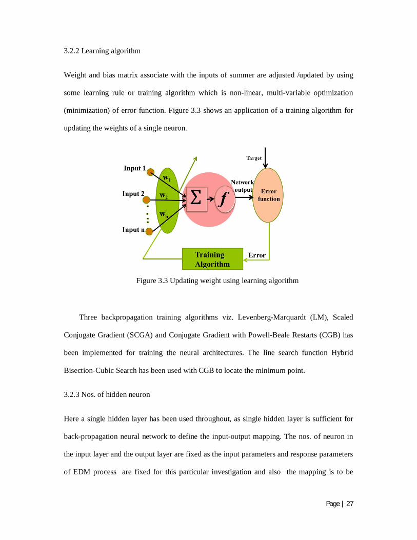
3.2.2 Learning algorithm…………………………………….

3.2.3 Nos. of hidden neuron…………………………………

3.2.4 Mean squared error…………………………………….

3.2.5 Correlation coefficient ………………………………...

3.3 Data collection………………………………………………

3.4 Important specifications……………………………………..

3.4.1 Data normalization……………………………………

3.4.2 Transfer /Activation function…………………………

3.5 Results and discussion from full factorial design

3.5.1. Effect on training MSE……………………………….

3.5.2 Effect on test MSE……………………………………

3.5.3 Effect on training R…………………………………...

3.5.4 Effect on testing R…………………………………….

3.6 Results and discussion from modelling……………………..

3.7 Conclusions………………………………………………….

25

26

26

27

28

29

34

34

35

39

41

43

45

47

53

4. Multi-Objective Optimization Comparison

4.1. Multi-objective optimization….............................................

4.1.2 MOO using NSGA-II………………………………...

4.1.2 MOO using Controlled NSGA-II…………………….

4.1.3 MOO using SPEA2…………………………………..

4.1.4 Comparison among algorithms………………………

4.2 Comparison

4.2.1. Diversity along the fronts……………………………

4.2.2. Domination of solutions……………………………..

4.3 Results and discussion………………………………….

4.3.1 Multi-objective optimization using

NSGA-II……………………………………………..

54

54

55

56

56

59 61

61

62

62

62

vii

CHAPTER

TITLE PAGE No

Controlled NSGA-II…………………………………

SPEA2……………………………………………….

4.3.2 Comparison…………………………………………..

4.3.3 Post-optimality analysis of Pareto-optimal solutions...

4.4 Conclusions…………………………………………………

65

67

69

73

76

5. Concluding Remarks………………………………………………... 77

6. Appendix……………………………………………………………. 78

7. Bibliography………………………………………………………… 81

viii

LIST OF FIGURES

Figure No. Figure Title Page

No.

Figure 1.1 Layout of Electric Discharge Machining 2

Figure 1.2: Variation of Ip and V in different phases of a spark 4

Figure 1.3 (a) Pre-breakdown phase (b) Breakdown phase (c) Discharge phase (d) End

of the discharge and (e) Post-discharge phase

5

Figure1.4(a) Neuron-anatomy of living animals 10

Figure1.4(b) Connection of an artificial Neuron 10

Figure 3.1 A general Network topology of MLP architecture 26

Figure 3.2 Common network topology of a CF neural architecture 26

Figure 3.3 Updating weight using Learning algorithm 27

Figure 3.4 Main effect plots for training MSE 39

Figure 3.5 Interaction plot for training MSE 40

Figure 3.6 Main effect plots for test MSE 41

Figure 3.7 Interaction plot for test MSE 42

Figure 3.8 Main effect plots for training R 43

Figure 3.9 Interaction plot for training R 44

Figure 3.10 Main effect plots for test R 45

Figure 3.11 Interaction plot for test R 46

Figure 3.12 ANN network topology of selected model 48

Figure 3.13 Variation of MSE w.r.t. epoch 48

Figure 3.14 Correlation coefficients 49

Figure 3.15 Variation of MRR and MRR output of training data w.r.t. exemplar 50

Figure 3.16 Variation of MRR and MRR output of testing data w.r.t. exemplar 52

Figure 3.17 Variation of TWR and TWR output of training data set w.r.t exemplar 51

Figure 3.18 Variation of TWR and TWR output of testing data set w.r.t exemplar 52

Figure 4.1 Flow chart representation of NSGA-II 57

Figure 4.2 Flow chart representation of Controlled NSGA-II 58

Figure 4.3 Flow chart representation of SPEA2 algorithm 60

ix

Figure No. Figure Title Page

No.

Figure 4.4 Pareto-optimal front obtained from NSGA-II 64

Figure 4.5 Pareto-optimal front obtained from Controlled NSGA-II 67

Figure 4.6 Pareto-optimal front obtained from SPEA2 69

Figure 4.7 Pareto-optimal fronts of different Algorithms 70

Figure 4.8 Histogram of Cnm in NSGA-II 72

Figure 4.9 Histogram of Cnm in CNGA-II 72

Figure 4.10 Histogram of Cnm in SPEA2 72

Figure 4.11 Effect of optimal process parameters on optimal MRR 74

Figure 4.12 Effect of optimal process parameters on optimal TWR 75

x

LIST OF TABLES

Table

No.

Table Title Page

No.

Table1.1 Lists of some MOEAs 8

Table1.2 Analogy between biological and artificial neurons 10

Table3.1 Parameters and their levels 24

Table3.2 Training data set 29

Table3.3 Validation data set 33

Table3.4 Test data set 33

Table 3.5 Important specification of parameters used in ANN modeling 34

Table3.6 Observation table for full factorial method 36

Table3.7 Analysis of Variance for training MSE 40

Table3.8 Analysis of Variance for test MSE 42

Table3.9 Analysis of Variance for Training R 44

Table3.10 Analysis of Variance for Test R 46

Table3.11 Weights and biases of optimal model (LM algorithm, 16 nos. of hidden

neurons and MLP neural architecture)

49

Table 4.1 Process parameter and functional setting of NSGA-II algorithm 56

Table 4.2 Optimal set of parameters obtained using NAGA-II 63

Table 4.3 Optimal sets of parameters obtained using Controlled NAGA-II 65

Table 4.4 Optimal sets of parameters obtained using SPEA2 67

Table 4.5 Maximum length factor values 70

Table 4.6 Mean of normalized cnm values 73

Table 4.7 Domination of percentage of solutions 73

xi

NOMENCLATURES

Asd Absolute deviation from standard mean

a2 Output vector of second layer

asl Output of neurons at hidden layer

Data mean of network output

an Network output at a particular examplar

ank Network output for exemplar n at neuron k of output layer

b1 Bias vector of first layer

b2 Bias vector of second layer respectively

Cnm Distance between two consecutive solutions

Data mean of desire output

dn Desire output at a particular exemplar

dnk Desired output for exemplar n at neuron k of output layer

dij distances in objective space

Average mean squared error function

E Mean squared error

( ) Mean squared error of training data set at epoch m

( ) Mean squared error of validation set error at epoch m

f The transfer function

Hessian matrix of average mean squared error function w.r.t. weights

Hessian matrix of average mean squared error function w.r.t. weights

Il The output of net-input function of l neurons

Ip Discharge current

Jacobian matrix of average mean squared error function w.r.t. weights

Jacobian matrix of average mean squared error function w.r.t. weights .

K Total number of neurons in the output layer

xii

N Population size

N Total number of exemplars in the data

Nmin and Nmax Minimum and maximum scaled range respectively

n Examplar or run number

p The input vector

Pt Parent population

Qt Child population

Rt Combined population

Rmin and Rmax Minimum and maximum values of the real variable respectively

Search directions for updating weights between hidden and output layer at epoch m

Search directions for updating weights between input and hidden layer at epoch m

Ton Spark on time

Tau Duty cycle

Weights between input and hidden layer

V Open circuit voltage

W1 Weight matrix of hidden layer

W2 Weight matrix of output layer

Weights between hidden and output layer

xiii

ACRONYMS

AMGA Archived-based Micro Genetic Algorithm

ANN Artificial Neural Network

CF Cascade-forward network

CG Conjugate gradient

CGB Conjugate Gradient with Powell-BealeRestarts

DE Dimensional Error

DPGA Distance-based Pareto Genetic Algorithm

EDM Electrical Discharge Machining

ES Evolutionary strategy

FEM Finite - element method

FPGA Fast Pareto Genetic Algorithm

GA Genetic Algorithm

GD Gradient descent

GFNN Generalized Feed forward Neural Network

IEG Inter Electrode Gap

IMOEA Intelligent Multi- Objective Evolutionary Algorithm

LM Levenberg Marquardt

MAE Mean absolute error

mBOA Multi-Objective Bayesian Optimization Algorithm

ME Mean error

MLP Multi-Layer Perceptron

MOEA Micro Genetic Algorithm

MOGA Multiple Objective Genetic Algorithm

MOMGA Multi-Objective Messy Genetic Algorithm

MOO Multi-Objective Optimization

MRR Material Removal Rate

MSE Mean square error

NCGA Neighborhood Cultivation Genetic Algorithm

NPGA Niched Pareto Genetic Algorithm

xiv

NSGA Non-dominated Sorting Genetic Algorithm

OC Over Cut

PAES Pareto Archived Evolutionary strategy

PESA Pareto Envelope-based Selection Algorithm

PG Population Genetics

SCG Scaled conjugate gradient

SCGA Scale Conjugate Gradient Algorithm

SPEA Strength Pareto Evolutionary Algorithm

SR Surface Roughness

SCD Surface Crack Density

TDGA Thermo-dynamical Genetic Algorithm

TWR Tool Wear Rate

VEGA Vector Evaluated Genetic Algorithm

VMRR Volumetric Material Removal Rate

VOES Vector Optimized Evolution Strategy

WLT White Layer Thickness

WBGA Weight-Based Genetic Algorithm

- MOEA - Multi- Objective Evolutionary Algorithm

Page | 1

CHAPTER1

INTRODUCTION

1.1 Introduction on EDM

Electrical Discharge Machining (EDM) is a non-conventional machining process, where

electrically conductive materials is machined by using precisely controlled sparks that occur

between an electrode and a workpiece in the presence of a dielectric fluid[1]. It uses thermo-

electric energy sources for machining extremely low machinability materials; complicated

intrinsic-extrinsic shaped jobs regardless of hardness have been its distinguishing characteristics.

EDM founds its wide applicability in manufacturing of plastic moulds, forging dies, press tools,

die castings, automotive, aerospace and surgical components. As EDM does not make direct

contact (an inter electrode gap is maintained throughout the process) between the electrode and

the workpiece it’s eradicate mechanical stresses, chatter and vibration problems during

machining [2].Various types of EDM process are available, but here the concern is about die-

Sinking (also known as ram) type EDM machines which require the electrode to be machined in

the exact opposite shape as the one in the workpiece [1].

1.1.1 Working principle of EDM

Electric discharge machining process is carried out in presence of dielectric fluid which creates

path for discharge. When potential difference is applied across the two surfaces of workpiece and

tool, the dielectric gets ionized and an electric spark/discharge is generated across the two

terminals. The potential difference is applied by an external direct current power supply

connected across the two terminals. The polarity of the tool and workpiece can be

interchangeable but that will affect the various performance parameters of EDM process. For

Page | 2

more material removal rate workpiece is generally connected to positive terminal as two third of

the total heat generated is generated near the positive terminal. The inter electrode gap has a

significant role to the development of discharge. As the workpiece remain fixed by the fixture

arrangement, tool helps in focusing the discharge or intensity of generated heat at the place of

shape impartment. Application of focused heat raises the temperature of workpiece in the region

of tool position, which subsequently melts and evaporates the metal. In this way the machining

process removes small volumes of workpiece material by the mechanism of melting and

vaporization during a discharge. The volume removed by a single spark is small, in the range of

10-6-10-4mm3, but this basic process is repeated typically 10,000 times per second.Figure 1.1

shows a layout of Electric Discharge Machining.

Figure 1.1: Layout of Electric Discharge Machining

Page | 3

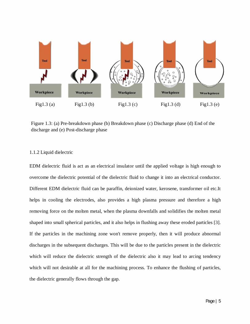
The erosion process due to a single electric spark in EDM generally passes through the following

phases and Figue 1.2 and 1.3 shows these phases:

(a) Pre-breakdown: In this phase the electrode moves close to the workpiece and voltage is

applied between the electrodes i.e. open circuit voltage Vo.

(b) Breakdown: When the applied voltage crosses the boundary limit of dielectric strength of

used dielectric fluid, the breakdown of the dielectric is initiated. Generally the dielectric starts

to break near the closest point between tool and workpiece, but it will also depend on conductive

particles between the gap if present any [3]. When the breakdown occurs the voltage falls and a

current rises abruptly. In this phase the dielectric gets ionized and a plasma channel is introduced

between the electrodes and also there is possibility of presence of current.

(c) Discharge:

In this phase the discharge current is maintained at constant level for a continuous bombardment

of ions and electrons on the electrodes. This will cause strong heating of the work-piece material

(and also of the electrode material), rapidly creating a small molten metal pool at the surface.

Also a small amount of metal can have directly vaporized due to the tremendous amount of heat.

During the discharge phase, the plasma channel grows; therefore the radius of the molten metal

pool also increases with time. In this phase some portion of the work-piece will be evaporated

and some will be remain in molten state. The Inter Electrode Gap (IEG) is an important

parameter throughout the discharge phase. It is estimated to be around 10 to 100 micrometers

(IEG increases with the increase in discharge current).

Page | 4

(d) End of the discharge:

At the end of the discharge, current and voltage supply is shut down. The plasma collapses (since

current is supply is stopped, there will be no more spark) under the pressure enforced by the

surrounding dielectric.

(e) Post-discharge:

There will be no plasma in this stage. Here a small portion of metal will be machined and a small

thin layer will be deposited because of plasma is collapsing and cooling. This layer is (20 to 100

microns) is known as white layer. Consequently, the molten metal pool is strongly sucked up

into the dielectric, leaving a small crater on the work-piece surface (typically 1-500 micrometer

in diameter, depending on the current).

Figure 1.2: Variation of Ip and V in different phases of a spark

Page | 5

1.1.2 Liquid dielectric

EDM dielectric fluid is act as an electrical insulator until the applied voltage is high enough to

overcome the dielectric potential of the dielectric fluid to change it into an electrical conductor.

Different EDM dielectric fluid can be paraffin, deionized water, kerosene, transformer oil etc.It

helps in cooling the electrodes, also provides a high plasma pressure and therefore a high

removing force on the molten metal, when the plasma downfalls and solidifies the molten metal

shaped into small spherical particles, and it also helps in flushing away these eroded particles [3].

If the particles in the machining zone won't remove properly, then it will produce abnormal

discharges in the subsequent discharges. This will be due to the particles present in the dielectric

which will reduce the dielectric strength of the dielectric also it may lead to arcing tendency

which will not desirable at all for the machining process. To enhance the flushing of particles,

the dielectric generally flows through the gap.

Fig1.3 (a) Fig1.3 (b) Fig1.3 (c) Fig1.3 (d) Fig1.3 (e)

Figure 1.3: (a) Pre-breakdown phase (b) Breakdown phase (c) Discharge phase (d) End of the discharge and (e) Post-discharge phase

Page | 6

1.1.3 Flushing

Flushing is the process of supplying clean filtered dielectric fluid into the machining zone. When

a dielectric is fresh, it is free from eroded particles and carbon residue resulting from dielectric

cracking and its insulation strength is high, but with successive discharges the dielectric gets

contaminated, reducing its insulation strength, and hence discharge can take place in an abrupt

manner. If the concentration of the particles became high at certain points within the IEG,

bridges are formed, which lead to abnormal discharges and damage the tool as well as the

workpiece.

There are different types of flushing methods like; injection flushing, suction flushing, side-

flushing, motion flushing and impulse flushing.

1.1.4 Machining parameters

For optimizing a machining process or to perform efficient machining one should have to

identify the process and performance measuring parameters. The machining parameter of EDM

process can be categorized into

(i) Input /process parameters: The input parameters of EDM process are voltage, discharge

current, spark-on time, duty factor, flushing pressure, work piece material, tool material,

inter-electrode gap, quill-up time, working time, and polarity which affects the

performance of machining process. So suitable selection of process parameters are

required for optimal machining condition.

(ii) Response /performance parameters: Response or performance parameters are used to

evaluate the machining process in both qualitative and quantitative terms namely

Material Removal Rate (MRR), Surface Roughness (Ra or SR), Over Cut (G or OC),

Page | 7

Tool Wear Rate (TWR), White Layer Thickness (WLT) and Surface Crack Density

(SCD).

1.2 Introduction on Evolutionary Multi-Objective Optimization(MOO)

A MOO generally deals with two or more objective functions which need to be optimized

simultaneously. Recently the evolutionary algorithms (based on the theory of Natural

Selection(NS) proposed by Darwin in 1859 and Population Genetics(PG) developed by

Fischer in 1930) are getting more familiar among the researchers due to its various

advantages like faster processing time, ability to deal with discontinuous search space, ability

to handle multi-modality of objectives and constraints etc.. Many of the recently developed

evolutionary algorithms have derived from the two original, independent concepts: the

evolutionary strategy (ES) developed by Richenberg in 1973 and Genetic Algorithm (GA)

proposed by Holland in 1975. Vector Evaluated Genetic Algorithm (VEGA) developed by

Schaffer in 1985 considered to be the first multi-objective evolutionary algorithm (MOEA)

which was a population based approach. Goldberg in1989 suggested the use of Pareto-based

approach fitness assignment strategy, where he suggested the use of non-dominated ranking

and selection to move the population towards the Pareto front. He also suggested about

niching mechanisms for diversity maintenance. Fonesca and Fleming in 1993 develop multi-

objective genetic algorithm (MOGA), based on Goldberg’s idea, which can be considered as

the first Pareto-based MOEA. The ranking method proposed by Fonesca and Fleming was

different from Goldberg’s. Some of MOEAs are listed below with the year of development in

Table 1.1.

Page | 8

Table 1.1 Lists of some MOEAs

Name of the MOEA Year of development

Vector Evaluated GA (VEGA) 1985

Lexicographic Ordering GA 1985

Vector Optimized Evolution Strategy (VOES) 1991

Weight-Based GA (WBGA) 1992

Multiple Objective GA (MOGA) 1993

Niched Pareto GA (NPGA, NPGA 2) 1993, 2001

Non-dominated Sorting GA (NSGA, NSGA-II, Controlled NSGA-II) 1994, 2000, 2001

Distance-based Pareto GA (DPGA) 1995

Thermo-dynamical GA (TDGA) 1996

Strength Pareto Evolutionary Algorithm (SPEA, SPEA2) 1999, 2001

Multi-Objective Messy GA (MOMGA-I,II,III) 1999, 2001,2003

Pareto Archived ES (PAES) 1999

Pareto Envelope-based Selection Algorithm (PESA, PESA II) 2000 ,2001

Micro GA-MOEA ( -GA, -GA2) 2001, 2003

Multi-Objective Bayesian Optimization Algorithm (mBOA) 2002

Neighborhood Cultivation Genetic Algorithm (NCGA) 2002

Intelligent Multi- Objective Evolutionary Algorithm (IMOEA) 2004

- Multi- Objective Evolutionary Algorithm ( -MOEA) 2005

Fast Pareto Genetic Algorithm (FPGA) 2007

Omni-Optimizer (OmniOpt) 2008

Archived-based Micro Genetic Algorithm (AMGA,AMGA2) 2008,2010

Page | 9

1.3 Introduction on Artificial Neural Network (ANN)

ANN refers to the computing systems whose fundamental concept is taken from analogy of

biological neural networks. Many day to day tasks involving intelligence or pattern recognition

are extremely difficult to automate, but appear to be performed very easily by animals. The

neural network of an animal is part of its nervous system, containing a network of specialized

cells called neurons (nerve cells). Neurons are massively interconnected, where an

interconnection is between the axon of one neuron and dendrite of another neuron. This

connection is referred to as synapse. Signals propagate from the dendrites, through the cell body

to the axon; from where the signals are propagate to all connected dendrites. A signal is

transmitted to the axon of a neuron only when the cell ‘fires’. A neuron can either inhibit or

excite a signal according to requirement.

Each artificial neuron receives signals from the environment, or other artificial neurons,

gather these signals, and when fired transmits a signal to all connected artificial neurons. Input

signals are inhibited or excited through negative and positive numerical weights associated with

each connection to the artificial neuron. The firing of an artificial neuron and the strength of the

exciting signal are controlled via. a function referred to as the activation function. The

summation function of artificial neuron collects all incoming signals, and computes a net input

signal as the function of the respective weights and biases. The net input signal serves as input to

the transfer function which calculates the output signal of artificial neuron.

Figure 1.4 (a) and (b) shows the analogy between biological and artificial neurons and the

analogy has been shown in parametric terms in Table 1.2.However ANN s are far too simple to

serve as realistic brain models on the cell levels, but they might serve as very good models for

the essential information processing tasks that organism perform.

Page | 10

Table1.2 Analogy between biological and artificial neurons

Biological Neurons Artificial Neurons

Soma or Cell body Summation function+ Activation function

Dendrite Input Axon Output Synapse Weight

Figure 1.4 (b) Connection of an artificial Neuron

Figure 1.4 (a) Neuron-anatomy of living animals

Page | 11

CHAPTER 2

LITERATURE REVIEW:

Relationship between process parameters and response parameters in EDM process are very

much stochastic, random and non-linear in nature. To establish a relation between input

parameters and output parameters various approaches like empirical relation, non-linear

regression, response surface methodology, neuro-fuzzy, neural network modeling etc. has been

investigated. Here in the primary phase a literature review has been done on modeling the EDM

process using ANN, to find out short comings if any and for investigating in the direction of

improvising the efficiency in ANN modeling of the EDM process. In the 2nd phase of literature

review, an investigation has been made on the implementation of ANN integrated GA based

multi-objective optimization on EDM process.

2.1 Literature review on ANN

As modeling of a process reduces the effort, save money and time for optimal and efficient

implementation of that process, it has a significant role in EDM process modeling also. Many

investigations already have been made in this direction using ANN modeling, but still its need

more improvement. So to identify the direction of improvement a literature review has been

made as follows:

Tsai and Wang [4] took six neural networks and a neuro-fuzzy network model for modeling

material removal rate (MRR) in EDM process and analyzed based on pertinent machine process

parameters. The networks, namely the LOGMLP, the TANMLP, the RBFN, the Error TANMLP,

the Adaptive TANMLP, the Adaptive RBFN, and the ANFIS have been trained and compared

under the same experimental conditions for two different materials considering the change of

polarity. The various neural network architectures that were used here for modelling were trained

Page | 12

with the same Gradient descent learning algorithm. For comparisons among the various models

various performance parameters like training time, RMSE, R2 were used. On the basis of

comparisons they found ANFIS model to be more accurate than the other models.

H. Juhr et. al [5] have made a comparison between NRF (nonlinear regression function )and

ANN for the generation of continuous parameter technology, which is a continuous mapping or

regression. They found ANN’s to much easier than NRF’s. For modeling with ANN’s, feed-

forward networks with three to five layers were used, which were trained with back-propagation

with momentum term. For developing the continuous parameter generation technology they

considered the input parameters as pulse current, discharge duration and duty cycle and response

parameters as removal rate, wear ratio and arithmetic mean roughness. They used two major

performance evaluation criteria sum of squared deviation and sum of relative deviation to

evaluate the performance of the two mapping functions. Finally they conclude that ANN shows

better prediction accuracy than nonlinear regression functions.

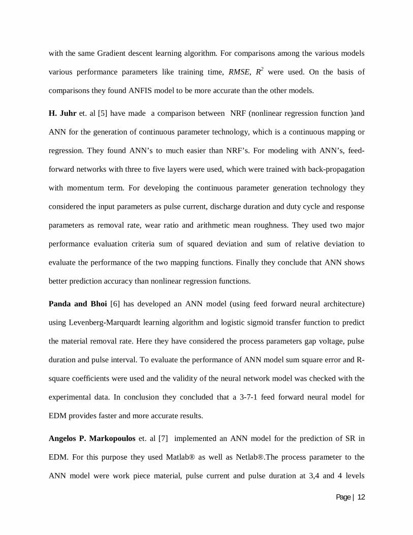
Panda and Bhoi [6] has developed an ANN model (using feed forward neural architecture)

using Levenberg-Marquardt learning algorithm and logistic sigmoid transfer function to predict

the material removal rate. Here they have considered the process parameters gap voltage, pulse

duration and pulse interval. To evaluate the performance of ANN model sum square error and R-

square coef cients were used and the validity of the neural network model was checked with the

experimental data. In conclusion they concluded that a 3-7-1 feed forward neural model for

EDM provides faster and more accurate results.

Angelos P. Markopoulos et. al [7] implemented an ANN model for the prediction of SR in

EDM. For this purpose they used Matlab® as well as Netlab®.The process parameter to the

ANN model were work piece material, pulse current and pulse duration at 3,4 and 4 levels

Page | 13

respectively. They used back propagation algorithm for training with model assessment criteria

as MSE and R. Finally they conclude that both Matlab® as well as Netlab® was found efficient

for prediction of SR of EDM process.

Assarzadeh and Ghoreishi [8] presented a research work on neural network modeling and

multi-objective optimization of responses MRR and SR of EDM process with Augmented

Lagrange Multiplier (ALM) algorithm. A 3–6–4–2-size back-propagation neural network was

developed to predict these two responses efficiently. The current (I), period of pulses (T), and

source voltage (V) were selected at 6, 4 and 4 levels respectively as network process parameters.

Out of 96 experimental data sets 82 data sets were used for training and remaining 14 data sets

were used for testing the network. The training model was trained with back propagation training

algorithm with momentum term. Relative percentage error and total average percentage error

were used to evaluate the models. From the results in terms of mean errors of 5.31% and 4.89%

in predicting the MRR and Ra they conclude that the neural model can predict process

performance with reasonable accuracy. Having established the process model, the augmented

Lagrange multiplier (ALM) algorithm was implemented to optimize MRR subjected to three

machining regimes of prescribed Ra constraints (i.e. finishing, semi-finishing and roughing) at

appropriate operating conditions.

Joshi and Pande [9] developed two models for the electric discharge machining (EDM) process

using the finite - element method (FEM) and artificial neural network (ANN). A two-

dimensional axisymmetric thermal (FEM) model of single-spark EDM process was developed

with the consideration of many thermo-physical characteristics to predict the shape of crater

cavity, MRR, and TWR. A multilayered feed-forward neural network with leaning algorithms

such as gradient descent (GD), GD with momentum (GDA), Levenberg – Marquardt (LM),

Page | 14

conjugate gradient (CG), scaled conjugate gradient (SCG) were employed to establish relation

between input process conditions (discharge power, spark on time, and duty factor) and the

process responses (crater geometry, material removal rate, and tool wear rate) for various

work—tool work materials. The input parameters and targets of the ANN model was generated

from the numerical (FEM) simulations. To evaluate the model they used prediction error(%) and

mean error (ME) and to improve the efficiency of model two BPNN architectures were tried out,

viz. single-layered (4 –N – 4) and two-layered (4 – N1 – N2 – 4). They found optimal ANN

model with network architecture 4 – 8 – 12 – 4 and SCG training algorithm to give very good

prediction accuracies for MRR (1.53%), crater depth (1.78%), and crater radius (1.16%) and a

reasonable one for TWR (17.34%).

M K Pradhan et. al [10] compared the performance and efficiency of back propagation neural

network (BPN) and radial basis function neural network (RBFN) for the prediction of SR in

EDM. Three process parameters i.e. pulses current (Ip), the pulse duration (Ton) and duty cycle

) were supplied to these two networks and corresponding experimental SR values were

considered as target. Out of the 44 experimental data sets, 35 nos. were considered for training

and remaining 9 data sets were considered for testing. They compared the performance of two

networks in terms of mean absolute error (MAE). MAE for test data of BPN and RBFN were

found to be 0.297188 and 0.574888 respectively, which indicates BPN to be more accurate. They

conclude that BPN is reasonably more accurate but RBFN is faster than the BPNs.

Promod Kumar Patowari et. al [11] have applied ANN to model material transfer rate (MTR)

and layer thickness (LT) by EDM with tungsten–copper (W–Cu) P/M sintered electrodes. They

have used input parameters to the ANN model such as compaction pressure (CP), sintering

temperature (ST), peak current (Ip), pulse on time (Ton), pulse off time (Toff) with target

Page | 15

measures like MTR, and LT. A multilayer feed-forward neural network with gradient-descent

learning algorithm with 5nos. of neuron in hidden layer has been used train the ANN model.

Two activation functions tansig and purelin has been used in hidden and output layers,

respectively. Two evaluate the ANN model two performance measures average error percentage

and MSE have implemented. The performance measure MSE during training and testing of MRR

were found to be 0.0014 and 0.0038, respectively. Another performance measure average error

percentage during training and testing of MRR were found to be 3.3321 and 8.4365, respectively.

While modeling LT, MSE during training and testing were found to be 0.0016 and 0.0020

respectively and average error percentage during training and testing were calculated to be

6.5732 and 3.1824 respectively.

Md. Ashikur Rahman Khan et. al [12] proposed an ANN model with multi-layer perception

neural architecture for the prediction of SR on first commenced Ti-15-3 alloy in electrical

discharge machining (EDM) process. The proposed models used process parameters such as

peak current, pulse on time, pulse off time and servo voltage to develop a mapping with the

target SR. Training of the ANN models was performed with LM learning algorithm using

extensive data sets from experiments utilizing copper electrode as positive polarity. An average

of 6.15% error was found between desired and ANN predicted SR which found to be in good

agreement with the experimental results.

Pushpendra S. Bharti et. al [13] made an attempt to select the best back propagation (BP)

algorithm from the list of training algorithms that are present in the Matlab Neural Network

Toolbox, for the training of ANN model of EDM process. In this work, thirteen BP algorithms,

which are available in MATLAB 7.1, Neural Network Toolbox, are compared on the basis of

mean absolute percentage error and correlation coe cient. Some important specifications that

Page | 16

have been used for implementing the ANN modeling were data normalization which was

performed in the range between 0.1 and 0.9, weight initialization which was done by Nguyen

Widrow weight initialization technique, transfer functions used at hidden layers and output layer

were hyperbolic tangent function (tansig) and logistic function (logsig) respectively. Out of

thirteen BP algorithms investigated, Bayesian Regularization Algorithm found to facilitate the

best results for efficient training of ANN model.

Pradhan and Das [14] have used an Elman network for producing a mapping between

machining parameter such as discharge current, pulse duration, duty cycle and voltage, and the

response MRR in EDM process. Training and testing of ANN model were performed with

extensive data sets from EDM experiments on AISI D2 tool steel from finishing, semi-finishing

to roughening operations. The mean percentage error of the model was found to be 5.86 percent,

which showed that the proposed model is in a satisfactory level to predict the MRR in EDM

process.

A.Thillaivannan [15] et. al. have explored a practical method of optimizing machining

parameters for EDM process under the minimum total machining time based on Taguchi method

and Artificial neural network. Feed-forward back-propagation neural networks with two back-

propagation training algorithms: gradient descent, and gradient descent with momentum were

developed for establishing a relation between the target parameters current and feed with the

process parameters required total machining time, oversize and taper of a hole .

Fenggou and Dayong [16] present a method that can be used to automatically determine the

optimal nos. of hidden neuron and optimize the relation between process and response

parameters of EDM process using GA and BP learning algorithm based ANN modelling. The

ANN modeling was implemented to establish relation between EDM process parameters such as

Page | 17

current peak value(A), pulse width on(µs) ,processing depth (mm) with the response parameters

SR(µm), TWR(%), electrode zoom value(µm) and finish depth(mm).A three layer feed forward

neural architecture was used to implement the ANN modeling in EDM process. The number of

neurons at the middle layer was determined by GA and node deleting network structure

optimization method. GA combined with node deleting network structure optimization method

was implemented to find out the global optimal solution, since it is hard for GA based

optimization method to find out the local optimal solution, a BP algorithm was nally

implemented to converge on the global optimum solution. AS GA converged to global optimal

solution quickly the training time is reduced now and as in the second phase BP algorithm was

implemented the local optimal solution problem also solved now. Finally they conclude 8 nos. of

hidden neuron were found to be optimal for ANN modeling with a desired processing precision

and efficiency.

Rao and Rao [17] presented a work aimed on the effect of various machining parameters on

hardness. The various input parameters that have been considered here are different types of

materials (namelyTi6Al4V, HE15, 15CDV6 and M250), current, voltage and machining time. To

correlate the machining parameters and response parameter they used a multi-layer feed forward

neural network with GA as a learning algorithm. For this purpose they used Neuro Solutions

software package. They used a single hidden layer with sigmoid transfer function in both hidden

and output layer. And they found a maximum prediction error of 5.42% and minimum prediction

error of 1.53%.

Deepak Kumar Panda [18] in this article, a new hybrid approach of neuro-grey modeling

(NGM) technique has been investigated for modeling and multi-optimization of multiple

processes attributes(SR, micro-hardness, thickness of heat affected zone, and MRR)of the electro

Page | 18

discharge machining (EDM) process. To establish an efficient relation between input parameters

pulse current and pulse duration with the response parameters of EDM process they used a multi-

layer feed forward neural network with Levenberg–Marquardt learning algorithm. The logistic

sigmoid transfer function was used in both hidden layer and output layer. For assessing the

performance of ANN model they used R2 and MSE performance measures.

Pradhan and Biswas [19] presented a research work, where two neuro-fuzzy models and a

neural network model were utilized for modelling of MRR, TWR, and radial overcut (G) of

EDM process for AISI D2 tool steel with copper electrode. The discharge current (Ip), pulse

duration (Ton), duty cycle ( ), and voltage (V) were taken as machining parameters. A feed-

forward neural network with one hidden layer and Levenberg–Marquardt as training algorithm

were used for implementing the ANN modeling. Weights were randomly initialized, and the

training, validation and testing data proportionate were taken as 50:40:10 respectively. The

performances of the developed models were measured in terms of Prediction error ( %) and

found to be 5.42, 15.21 and 6.51 percentage for testing data set of MRR,TWR and G respectively

which seems to approximate the responses quite accurately.

2.2 Literature review on implementation of MOEA

Development of MOEA has been started since last few decades and still it’s continuing in the

developing stage. In recent years many researchers have shown keen interest in the

implementation of MOEA, but till now it has not get wide applicability. Some of the

implementation has been presented below as literature review:

Kodali et. al [20] have shown an investigation on implementation of NSGA-II for optimizing

two contradicting responses in rough and finish grinding processes. For rough grinding

Page | 19

process minimizing the total production cost (CT) and maximizing the workpiece removal

parameter (WRP) were evaluated while for finish grinding process minimizing the total CT and

minimizing the surface roughness (Ra) were considered subjected to three constraints thermal

damage, wheel wear parameter and machine tool stiffness.

Kesheng Wang et. al [21] have employed a hybrid artificial neural network and Genetic

Algorithm methodology for modeling and optimization of two responses i.e. MRR and SR of

electro-discharge machining. To perform the ANN modeling and multi-objective optimization

they have implemented a two-phase hybridization process. In the first phase, they have used GA

as learning algorithm in multilayer feed-forward neural network architecture. In the second

phase, they used the model equations obtained from ANN modeling as the fitness functions for

the GA-based optimization. The optimization was implemented using Gene-Hunter. The ANN

model optimized error for MRR and SR were found to be 5.60% and 4.98% which laid a

conclusions for these two responses to accept the model.

J. C. Su et. al [22] have proposed a ANN integrated GA-based multi-objective optimization

system for optimization of machining performance parameters in an EDM process. A neural-

network model with back-propagation learning algorithm was developed to establish a relation

between the 8 process parameters such as pulse-on time (Ton), pulse-off time (Toff), high-voltage

discharge current (Ihv), low-voltage discharge current (Ilv), gap size (Gap), servo-feed (Vf),

jumping time (Tjump) and working time (Tw), and 3 response parameters Ra (the central-line

average roughness of the machined surface), the TWR and the MRR .As one hidden layer is

sufficient for ANN modeling of EDM process , they have used a 8-14-3 type feed- forward

neural network for modeling. After ANN modeling GA-based multi-objective optimization was

implemented using a composite objective function formed by ANN model equations. In the

Page | 20

composite objective function weights were introduced to re ect the importance of Ra, TWR and

MRR. From the verification and discussion they confirmed the successful applicability of GA-

based neural network for the optimization of the EDM process.

Joshi and Pande [23] reported an intelligent approach for modeling and multi-objective

optimization of EDM parameters of the model with less dependency on the experimental data.

The EDM parameters data sets were generated from the numerical (FEM) simulations. The

developed ANN process model was used in defining the fitness functions of non-dominated

sorting genetic algorithm II (NSGA-II) to select optimal process parameters for roughing and

finishing operations of EDM. While implementing NSGA-II for roughening operation only two

contradicting objectives MRR and TWR were considered, while implementing for finishing

operation best trade up was shared between 3 conflicting objective namely MRR, TWR and

crater depth. Finally they carried out a set of experiments to validate the process performance

for the optimum machining conditions and they found to be successful implement their approach.

Debabrata Mandal et. al [24] have presented a study attempts to model and optimize the EDM

process using a back-propagation neural network which uses a gradient search technique and a

GA based most familiar multi-objective optimization technique NSGA-II respectively. The

modeling has been established between 3 process parameters namely current, Ton and Toff with

responses MRR (mm3/min) Absolute tool wear rate (mm3/min).To nd out the suitable

architecture for an efficient ANN modeling of EDM process different architectures have been

investigated. The model with 3-10-10-2 architecture was found to be most suitable for the

modeling task with learning rate as 0.6 and momentum co-ef cient as 0.6. A total of 78nos. of

experimental run was used, out of which 69 nos. of run were used for training, and remaining 9

were used for testing the model. The maximum, minimum and mean prediction errors for this

Page | 21

model were found to be 9.47, 0.0137 and 3.06%, respectively. A multi-objective optimization

method NSGA -II was used to optimize the two conflicting responses MRR and TWR. Finally a

hundred nos. of Pareto-optimal solutions were successfully generated using NSGA-II.

Kuriakose and Shunmugam [25] correlate the various machining parameters and performance

parameters of wire-electro discharge machining using multiple linear regression model. The

various process parameters that were considered were namely ignition pulse current (IAL), time

between two pulses (TB), pulse duration (TA), servo-control reference voltage, maximum servo-

speed variation (S), wire speed (Ws), wire tension (Wb) and injection pressure (Inj).Two

contradicting responses of Wire-electro discharge machining process namely cutting velocity

and surface nish were taken into consideration for multi-objective optimization with the help of

Non-Dominated Sorting Genetic Algorithm (NSGA).The developed multiple linear regression

model equations were used as fitness functions in NSGA for performing the optimization task

and successfully implemented.

Kuruvila and Ravindra [26] developed a regression analysis method to correlate the machining

parameters pulse-on duration, current, bed speed, pulse-off duration and flush rate with the

response parameters Dimensional Error (DE), SR and Volumetric Material Removal Rate

(VMRR). The multi-objective optimization was performed using genetic algorithm .As GA is

basically implemented for single objective optimization; here a suitable modification was

pursued to implement it for multi-objective optimization. The modification was, forming a

composite objective function with consideration of weightage for different individual objectives,

which acts as fitness function for GA. Finally they conclude with the successful implementation

of this approach.

Page | 22

MahdaviNejad [27] has demonstrated the effective machining of Silicon Carbide (SiC) which is

regarded as a harder material, in EDM. Using ANN with a multilayer-perceptron (3-5-5-2)

architecture and back propagation algorithm the process parameters discharge current, pulse on

time, pulse off time have been mapped with the two responses SR and MRR. For optimizing the

process parameters simultaneously w.r.t. the objectives SR and MRR, NSGA-II algorithm was

applied and a set of non-dominated solutions were achieved.

From the literature review it was confirmed that efficiency of ANN still needs to be

improvised. Many of the researchers have randomly selected the process parameters (and their

value) of ANN for developing an efficient model for their particular purpose of implementations.

So here, there is a high necessity of developing an orderly manner for selecting process

parameters and their levels for improving the performance of ANN.

Through study of literature review reveals that many MOEAs have been implemented for

MOO of EDM process, but still now no comparison has been made about the performance of

various MOEAs. So an investigation is required on this to evaluate and compare various

MOEAs, in qualitative and quantitative parametric terminologies.

Page | 23

2.3 Objective of present work

A three step frame work was prepared for conceptualizing the research direction as follows:

1. To study the performance of ANN process parameters ANN architectures,

Learning/training algorithms and Nos. of hidden neurons with the help of full factorial

design.

2. Optimal process modeling of MRR and TWR of EDM process with the best levels of

these above parameters.

3. Multi-objective optimization of EDM responses using three wide applied MOEAs,

namely Non-dominated Sorting Genetic Algorithm-II (NSGA-II),Controlled NSGA-II

and Strength Pareto Evolutionary Algorithm 2 (SPEA2) .

Page | 24

CHAPTER 3

ANN Performance Evaluation and Modelling

Many attempts have been made to model performance parameters of EDM process using

ANN.To obtain an improved ANN model, generally ANN architectures, learning/training

algorithms and nos. of hidden neurons are varied, but the variation so far has been made in a

random manner. So here a full factorial design has been implemented to achieve the optimal

of above for modelling.

3.1 Parameter setting

The most familiar process parameters that are varied to obtain an efficient ANN model are

ANN architectures; learning/training algorithms and nos. of hidden neuron. These parameters

have been chosen here as process parameters to a full factorial design. The process parameter

ANN architecture at two levels, learning/training algorithm at three levels and nos. of hidden

neuron at four levels have been selected as shown in Table 3.1. The performance parameters

for evaluating the ANN model are taken as training Mean squared error ( MSE), testing MSE,

training Correlation coefficient (R) and testing R, which are the default performances

evaluating parameters assumed by MATLAB.

Table 3.1 Parameters and their levels

Process parameter Levels

1 2 3 4

Neural Architecture Multi-Layer Perceptron (MLP)

Generalized Feed forward Neural Network (GFNN)

Learning Algorithm Levenberg Marquardt (LM)

Scale Conjugate Gradient Algorithm (SCGA)

Conjugate Gradient with Powell-Beale Restarts (CGB)

Nos. of hidden neuron 8 16 24 32

Page | 25

3.2 About the parameters

3.2.1 Neural architecture

A single neuron is not enough to solve real life problems (any linear or nonlinear

computation) efficiently, and networks with more number of neurons arranged in particular

sequences are frequently required. This particular ways /sequences of arrangement of neurons

are coined as neural architecture. The sequences of arrangements of neurons determine how

computations will proceed and also responsible for the effectiveness of the model.

Multi-layer perceptron (MLP):

A multilayer perceptron neural architecture has one or more layers of nodes/neurons (hidden

layers) between the input and output layers. Here discharge current (Ip), spark on time (Ton),

duty cycle (Tau) and voltage (V) are the processing parameters comprising the input layer.

The output layer comprises of two neurons representing the two response parameters material

removal rate (MRR) and tool wear rate (TWR). The hidden layers are so called because they

are not exposed to the external environment (data) and it is not possible to examine and

correct their values directly. A general network topology of MLP neural architecture has been

shown in Figure 3.1.

Cascade-forward network (CF) / Generalize feed-forward network (GFNN):

Generalized feed-forward networks are a generalization of the MLP such that weight

connection can jump over from the input to each layer and from each layer to the successive

layers. The additional connections have been added in the hope of solving the problem much

more efficiently and faster manner. Network topology of a general CF neural architecture has

been shown in Figure 3.2.

Page | 26

Figure 3.1 A general Network topology of MLP architecture

Figure 3.2 Common network topology of a CF neural architecture

Page | 27

Figure 3.3 Updating weight using learning algorithm

3.2.2 Learning algorithm

Weight and bias matrix associate with the inputs of summer are adjusted /updated by using

some learning rule or training algorithm which is non-linear, multi-variable optimization

(minimization) of error function. Figure 3.3 shows an application of a training algorithm for

updating the weights of a single neuron.

Three backpropagation training algorithms viz. Levenberg-Marquardt (LM), Scaled

Conjugate Gradient (SCGA) and Conjugate Gradient with Powell-Beale Restarts (CGB) has

been implemented for training the neural architectures. The line search function Hybrid

Bisection-Cubic Search has been used with CGB to locate the minimum point.

3.2.3 Nos. of hidden neuron

Here a single hidden layer has been used throughout, as single hidden layer is sufficient for

back-propagation neural network to define the input-output mapping. The nos. of neuron in

the input layer and the output layer are fixed as the input parameters and response parameters

of EDM process are fixed for this particular investigation and also the mapping is to be

Page | 28

established between input and output parameters .So to investigate the effect of nos. neuron

on model performance nos. of hidden neuron has been varied at four levels.

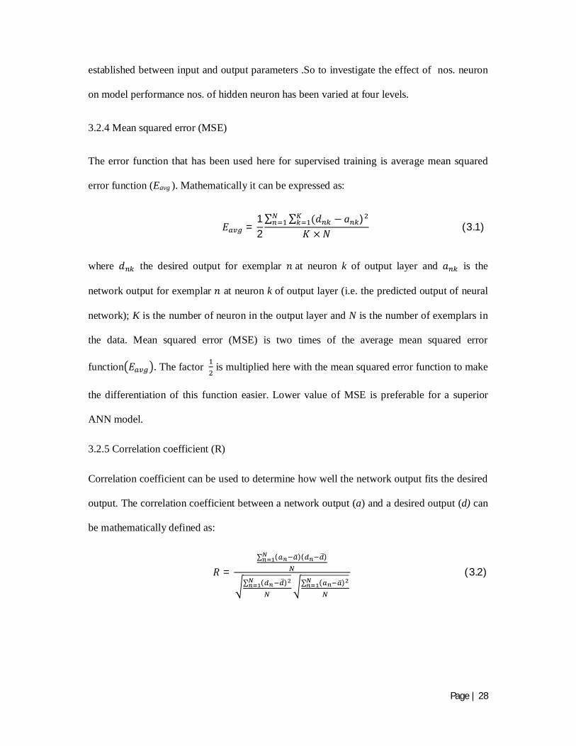
3.2.4 Mean squared error (MSE)

The error function that has been used here for supervised training is average mean squared

error function (Eavg ). Mathematically it can be expressed as:

=12

a )(3.1)

where the desired output for exemplar at neuron k of output layer and is the

network output for exemplar at neuron k of output layer (i.e. the predicted output of neural

network); K is the number of neuron in the output layer and N is the number of exemplars in

the data. Mean squared error (MSE) is two times of the average mean squared error

function . The factor is multiplied here with the mean squared error function to make

the differentiation of this function easier. Lower value of MSE is preferable for a superior

ANN model.

3.2.5 Correlation coefficient (R)

Correlation coefficient can be used to determine how well the network output fits the desired

output. The correlation coefficient between a network output (a) and a desired output (d) can

be mathematically defined as:

=( )( )

( ) ( )(3.2)

Page | 29

(continued on next page)

where n = examplar or run number, an and dn are the network output and desire output

respectively at a particular examplar, and are the data mean of network output and desire

output respectively. Higher value of R is desirable for an effective ANN model.

3.3 Data (machining parameters) collection:

The process parameters and response parameters data of the EDM process used here for

modeling is referred with permission from Pradhan [28].

The total nos. of exemplar in the data set is 150.The whole data set was divided into 3

sets viz. training,validation and test dataset.The training data set is used to fit the model or to

establish the input-output mapping.The validation data set is used stop the training by early

stopping criteria. Test data set is used to evaluate the performance and generalization error of

fully trained neural network model. Generalization means how well the trained model

response to the data set that does not belong to the training set.

The training, validation and test data set was respectively proportionate to 80:10:10.

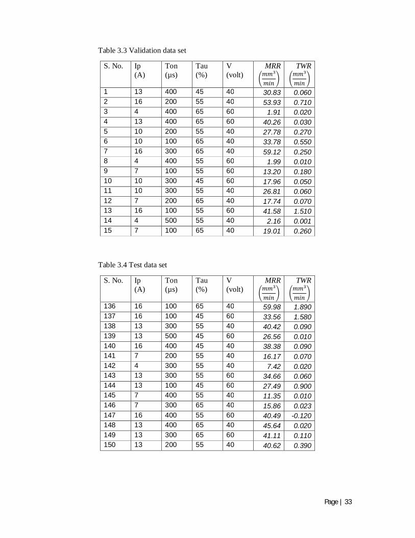
Table 3.2 ,3.3 and 3.4 shows the training, validation and tesing dataset respectivly.

Table 3.2 Training data set

S. No. Ip (A)

Ton (µs)

Tau (%)

V (volt)

MRR

TWR

1 10 500 55 60 17.50 -0.010 2 7 200 65 60 14.73 0.070 3 7 100 55 40 16.34 0.160 4 10 200 45 60 19.09 0.150 5 16 400 55 40 51.01 0.020 6 13 100 55 40 40.92 0.980 7 16 500 55 60 39.36 -0.110 8 16 300 65 60 47.96 0.170 9 4 300 55 60 4.23 0.020 10 4 400 55 40 4.74 0.020 11 16 300 55 60 40.90 0.080 12 10 300 65 60 24.90 0.060

Page | 30


S. No. Ip (A)

Ton (µs)

Tau (%)

V (volt)

MRR

TWR

13 10 400 65 40 29.07 0.010 14 16 500 45 60 31.13 0.010 15 10 100 65 60 26.66 0.650 16 7 300 45 60 9.08 0.040 17 7 400 55 60 8.79 0.030 18 16 400 65 40 57. 68 0.090 19 7 200 45 40 13.57 0.080 20 10 500 65 40 28.27 -0.020 21 13 200 65 40 49.05 0.420 22 7 400 65 40 13.70 0.010 23 7 300 65 60 12.75 0.030 24 10 500 65 60 19.92 0.001 25 4 500 65 40 2.01 0.001 26 4 400 65 40 4.43 0.010 27 16 200 45 60 32.91 0.550 28 16 200 65 60 48.29 0.490 29 10 300 55 60 22.16 0.070 30 4 300 45 60 3.32 0.020 31 16 200 55 60 41.26 0.520 32 10 200 55 60 22.74 0.190 33 10 200 65 40 33.05 0.140 34 16 500 45 40 37.52 0.030 35 16 100 55 40 54.15 1.780 36 10 400 45 40 20.96 0.040 37 10 500 45 40 19.04 0.010 38 4 500 45 40 2.12 0.010 39 4 100 55 60 5.61 0.100 40 16 400 45 60 32.39 0.050 41 7 100 65 60 16.29 0.310 42 7 200 55 60 13.08 0.080 43 7 100 45 40 14.50 0.190 44 4 200 55 40 7.93 0.010 45 4 100 45 40 5.77 0.070 46 13 100 55 60 36.09 0.790 47 13 500 55 40 38.06 -0.100 48 10 400 65 60 22.25 0.020 49 16 300 55 40 53.06 0.200 50 16 400 65 60 47.38 0.080 51 16 500 65 40 56.57 0.060 52 13 100 45 40 32.96 1.020 53 4 500 45 60 1.70 0.001 54 10 400 45 60 16.43 0.020

Page | 31


S. No. Ip (A)

Ton (µs)

Tau (%)

V (volt)

MRR

TWR

55 13 200 45 60 27.23 0.300 56 4 500 65 60 1.46 0.001 57 7 300 55 60 12.31 0.060 58 4 300 65 60 3.13 0.010 59 7 100 45 60 11.99 0.190 60 4 400 45 60 2.38 0.010 61 4 300 65 40 5.75 0.001 62 10 200 65 60 25.49 0.150 63 13 400 55 40 39.69 0.010 64 10 100 45 40 23.48 0.630 65 16 100 45 40 39.81 1.800 66 4 200 65 60 5.80 0.020 67 13 500 45 40 30.29 0.020 68 10 500 55 40 23.95 -0.060 69 4 500 55 60 1.34 0.010 70 10 100 45 60 19.36 0.420 71 13 100 65 40 49.27 1.040 72 7 300 45 40 12.81 0.040 73 4 200 55 60 5.04 0.040 74 7 400 45 40 11.03 0.020 75 13 400 45 60 26.90 0.020 76 10 400 55 40 25.55 0.030 77 13 300 45 40 31.82 0.120 78 7 500 45 40 9.03 0.010 79 10 400 55 60 20.36 0.020 80 4 400 45 40 2.83 0.010 81 16 300 45 60 32.66 0.090 82 13 300 65 40 48.33 0.170 83 7 200 45 60 10.75 0.090 84 16 500 55 40 49.40 -0.070 85 7 500 65 60 7.00 0.010 86 10 500 45 60 15.60 0.001 87 4 100 45 60 5.53 0.100 88 13 200 65 60 41.62 0.260 89 13 400 55 60 34.36 0.001 90 7 500 55 60 6.59 0.010 91 16 100 65 60 48.54 1.700 92 4 100 65 60 6.87 0.090 93 4 200 65 40 6.74 0.010 94 16 200 65 40 59.79 0.560 95 4 100 65 40 8.22 0.040 96 13 500 55 60 31.97 -0.090

Page | 32

S. No. Ip (A)

Ton (µs)

Tau (%)

V (volt)

MRR

TWR

97 10 200 45 40 22.52 0.190 98 10 100 55 40 28.08 0.570 99 13 100 65 60 42.09 1.080 100 10 100 55 60 23.05 0.440 101 16 500 65 60 46.49 0.040 102 7 500 45 60 5. 93 0.001 103 7 400 65 60 9.78 0.020 104 13 300 45 60 27.11 0.080 105 4 300 45 40 3.53 0.020 106 4 100 55 40 8.24 0.080 107 13 500 65 60 38. 03 0.020 108 7 400 45 60 7.23 0.010 109 13 200 55 60 35.23 0.300 110 13 200 45 40 32.79 0.310 111 10 300 45 40 21.97 0.060 112 10 300 65 40 31.25 0.030 113 7 500 55 40 8.43 -0.010 114 16 200 45 40 39.56 0.640 115 4 200 45 60 4.60 0.070 116 7 500 65 40 10.14 -0.020 117 16 300 45 40 38.54 0.210 118 7 300 55 40 15.20 0.040 119 13 500 65 40 43.04 0.001 120 4 200 45 40 4.91 0.040

Page | 33

Table 3.3 Validation data set

S. No. Ip (A)

Ton (µs)

Tau (%)

V (volt)

MRR

TWR

1 13 400 45 40 30.83 0.060 2 16 200 55 40 53.93 0.710 3 4 400 65 60 1.91 0.020 4 13 400 65 60 40.26 0.030 5 10 200 55 40 27.78 0.270 6 10 100 65 40 33.78 0.550 7 16 300 65 40 59.12 0.250 8 4 400 55 60 1.99 0.010 9 7 100 55 60 13.20 0.180 10 10 300 45 60 17.96 0.050 11 10 300 55 40 26.81 0.060 12 7 200 65 40 17.74 0.070 13 16 100 55 60 41.58 1.510 14 4 500 55 40 2.16 0.001 15 7 100 65 40 19.01 0.260

Table 3.4 Test data set

S. No. Ip (A)

Ton (µs)

Tau (%)

V (volt)

MRR

TWR

136 16 100 65 40 59.98 1.890 137 16 100 45 60 33.56 1.580 138 13 300 55 40 40.42 0.090 139 13 500 45 60 26.56 0.010 140 16 400 45 40 38.38 0.090 141 7 200 55 40 16.17 0.070 142 4 300 55 40 7.42 0.020 143 13 300 55 60 34.66 0.060 144 13 100 45 60 27.49 0.900 145 7 400 55 40 11.35 0.010 146 7 300 65 40 15.86 0.023 147 16 400 55 60 40.49 -0.120 148 13 400 65 40 45.64 0.020 149 13 300 65 60 41.11 0.110 150 13 200 55 40 40.62 0.390

Page | 34

3.4 Important specifications used for ANN modelling

Some of the important specifications of parameters that are frequently required throughout

the modeling process have been shown in Table 3.5.

Table 3.5 Important specification of parameters used in ANN modelling

S.N. Parameter Data/ Data range

Technique used/ Type of Parameter used

1. Nos. of input neuron 4 ____________ 2. Nos. of output neuron 2 ____________

3. Total nos. of exemplar 150 ____________ 4. Proportion of training,

validation & testing data 80:10:10 ____________

5. Data normalization 0.05 to 0.95 Min-max data normalization technique

6. Weight initialization -0.5 to 0.5 Random weight initialization technique

7. Transfer function 0 and 1 Log-sigmoid function (for both hidden & output layer)

8. Error function ___________ Mean squared error function

9. Mode of training ___________ Batch mode

10. Type of Learning rule ___________ Supervised learning rule

11. Stopping criteria ___________ Early stopping

Two important parameters, data normalization and transfer function also have been described

below:

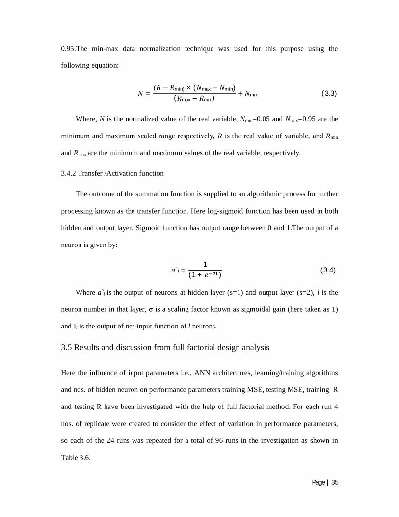
3.4.1 Data normalization:

Generally the inputs and targets that dealt with an ANN model are of various ranges. These

input and targets are needed to be scaled in the same order of magnitude otherwise some

variables may appear to have more significance than they actually do, which will lead to form

error in the model. Here the data of neural network model was scaled in the range of 0.05 to

Page | 35

0.95.The min-max data normalization technique was used for this purpose using the

following equation:

=min) × ( max min)( max min) min (3.3)

Where, N is the normalized value of the real variable, Nmin=0.05 and Nmax=0.95 are the

minimum and maximum scaled range respectively, R is the real value of variable, and Rmin

and Rmax are the minimum and maximum values of the real variable, respectively.

3.4.2 Transfer /Activation function

The outcome of the summation function is supplied to an algorithmic process for further

processing known as the transfer function. Here log-sigmoid function has been used in both

hidden and output layer. Sigmoid function has output range between 0 and 1.The output of a

neuron is given by:

sl =

1(1 + l) (3.4)

Where asl is the output of neurons at hidden layer (s=1) and output layer (s=2), l is the

neuron number in that layer, is a scaling factor known as sigmoidal gain (here taken as 1)

and Il is the output of net-input function of l neurons.

3.5 Results and discussion from full factorial design analysis

Here the influence of input parameters i.e., ANN architectures, learning/training algorithms

and nos. of hidden neuron on performance parameters training MSE, testing MSE, training R

and testing R have been investigated with the help of full factorial method. For each run 4

nos. of replicate were created to consider the effect of variation in performance parameters,

so each of the 24 runs was repeated for a total of 96 runs in the investigation as shown in

Table 3.6.

Page | 36

Table 3.6 Observation table for full factorial method

Run Order

Neural Arch.

Learning Algorithm

Nos. of Hidden Neuron

Training MSE

Test MSE

Training R

Test R

1 MLP CGB 8 0.2815 0.5432 0.99946 0.99923 2 MLP CGB 16 0.1016 0.3915 0.99981 0.99953 3 MLP CGB 24 0.0846 0.4139 0.99984 0.99943 4 MLP CGB 32 0.0762 0.2803 0.99985 0.99961 5 MLP LM 8 0.1420 0.4390 0.99973 0.99940 6 MLP LM 16 0.0241 0.1529 0.99995 0.99980 7 MLP LM 24 0.0071 0.3597 0.99999 0.99955 8 MLP LM 32 0.0031 0.4650 0.99999 0.99938 9 MLP SCGA 8 0.3418 0.7741 0.99934 0.99891 10 MLP SCGA 16 0.1157 0.3637 0.99978 0.99957 11 MLP SCGA 24 0.1100 0.6763 0.99979 0.99932 12 MLP SCGA 32 0.1017 0.7141 0.99980 0.99927 13 CF CGB 8 0.2914 0.4753 0.99944 0.99943 14 CF CGB 16 0.1243 0.4552 0.99976 0.99948 15 CF CGB 24 0.1077 0.5426 0.99979 0.99943 16 CF CGB 32 0.0891 0.4977 0.99983 0.99945 17 CF LM 8 0.0850 0.3334 0.99984 0.99956 18 CF LM 16 0.0196 0.2031 0.99996 0.99972 19 CF LM 24 0.0030 0.8960 0.99999 0.99915 20 CF LM 32 0.0018 0.5012 1.00000 0.99952 21 CF SCGA 8 0.1782 0.6252 0.99966 0.99919 22 CF SCGA 16 0.1011 0.3603 0.99981 0.99954 23 CF SCGA 24 0.0977 0.3968 0.99981 0.99959 24 CF SCGA 32 0.0887 0.7101 0.99983 0.99930 25 MLP CGB 8 0.3236 0.4869 0.99938 0.99935 26 MLP CGB 16 0.0982 0.2604 0.99981 0.99963 27 MLP CGB 24 0.0548 0.3808 0.99989 0.99961 28 MLP CGB 32 0.0599 0.4621 0.99988 0.99939 29 MLP LM 8 0.1226 0.4955 0.99976 0.99934 30 MLP LM 16 0.0236 0.2042 0.99995 0.99972 31 MLP LM 24 0.0074 0.2503 0.99999 0.99966 32 MLP LM 32 0.0009 0.6482 1.00000 0.99938 33 MLP SCGA 8 0.3240 0.7849 0.99938 0.99889 34 MLP SCGA 16 0.1235 0.2791 0.99976 0.99961 35 MLP SCGA 24 0.1100 0.6763 0.99979 0.99932 36 MLP SCGA 32 0.0690 0.5977 0.99987 0.99948 37 CF CGB 8 0.3052 0.4736 0.99941 0.99938 38 CF CGB 16 0.1438 0.2264 0.99972 0.99971 39 CF CGB 24 0.1187 0.5340 0.99977 0.99948 40 CF CGB 32 0.0819 0.6060 0.99984 0.99921

Page | 37

Run Order

Neural Arch.

Learning Algorithm


Training MSE

Test MSE

Training R

Test R

41 CF LM 8 0.1017 0.2025 0.99980 0.99972 42 CF LM 16 0.0105 0.3858 0.99998 0.99952 43 CF LM 24 0.0035 0.8005 0.99999 0.99914 44 CF LM 32 0.0021 0.4612 1.00000 0.99958 45 CF SCGA 8 0.1632 0.4960 0.99969 0.99934 46 CF SCGA 16 0.1100 0.3412 0.99979 0.99954 47 CF SCGA 24 0.0673 0.5468 0.99987 0.99944 48 CF SCGA 32 0.0660 0.6247 0.99987 0.99918 49 MLP CGB 8 0.2843 0.5215 0.99945 0.99931 50 MLP CGB 16 0.0976 0.3323 0.99981 0.99958 51 MLP CGB 24 0.0683 0.4742 0.99987 0.99939 52 MLP CGB 32 0.0650 0.4749 0.99988 0.99940 53 MLP LM 8 0.1207 0.3403 0.99977 0.99954 54 MLP LM 16 0.0223 0.1946 0.99996 0.99972 55 MLP LM 24 0.0029 0.3201 0.99999 0.99959 56 MLP LM 32 0.0003 0.5428 1.00000 0.99946 57 MLP SCGA 8 0.3251 0.7695 0.99938 0.99893 58 MLP SCGA 16 0.1536 0.4952 0.99971 0.99949 59 MLP SCGA 24 0.0726 0.4786 0.99986 0.99947 60 MLP SCGA 32 0.0589 0.6425 0.99989 0.99937 61 CF CGB 8 0.2968 0.5738 0.99943 0.99925 62 CF CGB 16 0.1695 0.4845 0.99967 0.99959 63 CF CGB 24 0.0954 0.4529 0.99982 0.99943 64 CF CGB 32 0.0775 0.5932 0.99985 0.99923 65 CF LM 8 0.1040 0.2852 0.99980 0.99962 66 CF LM 16 0.0184 0.4988 0.99996 0.99952 67 CF LM 24 0.0032 0.9699 0.99999 0.99908 68 CF LM 32 0.0024 0.6140 1.00000 0.99937 69 CF SCGA 8 0.1880 0.5374 0.99964 0.99926 70 CF SCGA 16 0.0927 0.1613 0.99982 0.99978 71 CF SCGA 24 0.1037 0.4336 0.99980 0.99940 72 CF SCGA 32 0.0848 0.4811 0.99984 0.99939 73 MLP CGB 8 0.3249 0.6884 0.99938 0.99930 74 MLP CGB 16 0.1156 0.3324 0.99978 0.99958 75 MLP CGB 24 0.0795 0.3719 0.99985 0.99952 76 MLP CGB 32 0.0209 0.3649 0.99996 0.99948 77 MLP LM 8 0.1348 0.4764 0.99974 0.99936 78 MLP LM 16 0.0124 0.1714 0.99998 0.99976 79 MLP LM 24 0.0059 0.1771 0.99999 0.99978 80 MLP LM 32 0.0015 0.5497 1.00000 0.99927 81 MLP SCGA 8 0.3036 0.6976 0.99942 0.99907 82 MLP SCGA 16 0.1372 0.4899 0.99974 0.99950

Page | 38

Run Order

Neural Arch.

Learning Algorithm


Training MSE

Test MSE

Training R

Test R

83 MLP SCGA 24 0.0688 0.4997 0.99987 0.99942 84 MLP SCGA 32 0.0584 0.7697 0.99989 0.99931 85 CF CGB 8 0.3142 0.5747 0.99940 0.99921 86 CF CGB 16 0.1099 0.3037 0.99979 0.99961 87 CF CGB 24 0.0889 0.4886 0.99983 0.99970 88 CF CGB 32 0.0651 0.5085 0.99988 0.99929 89 CF LM 8 0.0842 0.2854 0.99984 0.99962 90 CF LM 16 0.0137 0.3267 0.99997 0.99954 91 CF LM 24 0.0062 0.7403 0.99999 0.99931 92 CF LM 32 0.0041 0.5950 0.99999 0.99943 93 CF SCGA 8 0.1728 0.4855 0.99967 0.99934 94 CF SCGA 16 0.0937 0.3482 0.99982 0.99951 95 CF SCGA 24 0.0621 0.4023 0.99988 0.99946 96 CF SCGA 32 0.0912 0.7927 0.99982 0.99931

Page | 39

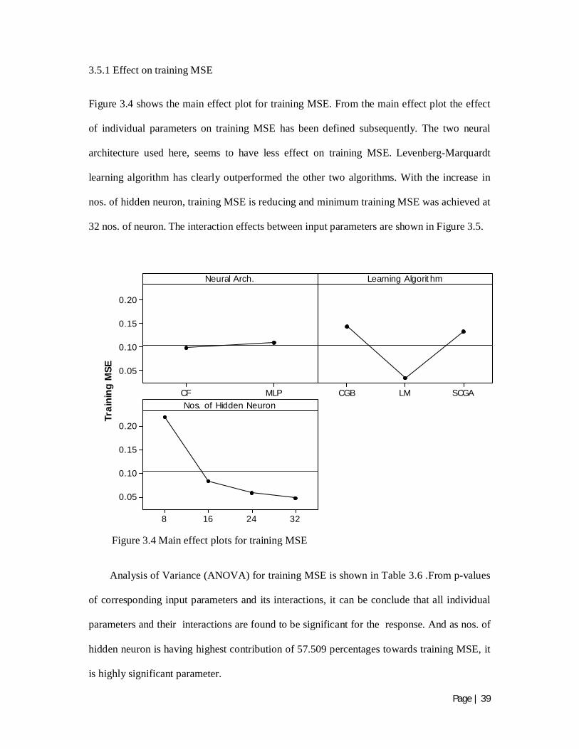
3.5.1 Effect on training MSE

Figure 3.4 shows the main effect plot for training MSE. From the main effect plot the effect

of individual parameters on training MSE has been defined subsequently. The two neural

architecture used here, seems to have less effect on training MSE. Levenberg-Marquardt

learning algorithm has clearly outperformed the other two algorithms. With the increase in

nos. of hidden neuron, training MSE is reducing and minimum training MSE was achieved at

32 nos. of neuron. The interaction effects between input parameters are shown in Figure 3.5.

MLPCF

0.20

0.15

0.10

0.05

SCGALMCGB

3224168

0.20

0.15

0.10

0.05

Neural Arch.

Trai

ning

MSE

Learning Algorithm


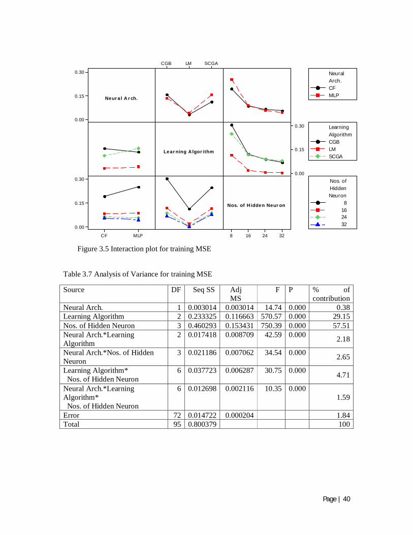
Analysis of Variance (ANOVA) for training MSE is shown in Table 3.6 .From p-values

of corresponding input parameters and its interactions, it can be conclude that all individual

parameters and their interactions are found to be significant for the response. And as nos. of

hidden neuron is having highest contribution of 57.509 percentages towards training MSE, it

is highly significant parameter.

Figure 3.4 Main effect plots for training MSE

Page | 40

0.30

0.15

0.00

3224168

SC GALMC GB

0.30

0.15

0.00

MLPC F

0.30

0.15

0.00

Neural A rch.

Learning A lgorithm

Nos. of Hidden Neur on

CFMLP

Arch.Neural

CGBLMSCGA

AlgorithmLearning

8162432

NeuronHiddenNos. of

Table 3.7 Analysis of Variance for training MSE

Source DF Seq SS Adj MS

F P % of contribution

Neural Arch. 1 0.003014 0.003014 14.74 0.000 0.38 Learning Algorithm 2 0.233325 0.116663 570.57 0.000 29.15 Nos. of Hidden Neuron 3 0.460293 0.153431 750.39 0.000 57.51 Neural Arch.*Learning Algorithm

2 0.017418 0.008709 42.59 0.000 2.18

Neural Arch.*Nos. of Hidden Neuron

3 0.021186 0.007062 34.54 0.000 2.65

Learning Algorithm* Nos. of Hidden Neuron

6 0.037723 0.006287 30.75 0.000 4.71

Neural Arch.*Learning Algorithm* Nos. of Hidden Neuron

6 0.012698 0.002116 10.35 0.000 1.59

Error 72 0.014722 0.000204 1.84 Total 95 0.800379 100

Figure 3.5 Interaction plot for training MSE

Page | 41

3.5.2 Effect on test MSE

Figure 3.6 shows the main effect plot for test MSE. From the figure assessments drawn are;

neural architecture has insignificant effect on test MSE, Levenberg-Marquardt training

algorithm and 16 nos. of neuron at hidden layer are liable for the lowest test MSE. Interaction

plot for test MSE has been shown in Figure 3.7.

MLPCF

0.55

0.50

0.45

0.40

0.35

SCGALMCGB

3224168

0.55

0.50

0.45

0.40

0.35

Neural Arch.

Test

MSE

Learning Algorithm


From the ANOVA for test MSE as shown in Table 3.7, it was found that all the

individual parameters except neural architecture have significant effects on test MSE. All the

interaction effects among the individual parameters also express significant effects towards

the test MSE at a significance level of 0.05. A major 28.03 percentage of contribution effect

was added to test MSE by nos. hidden neurons.

Figure 3.6 Main effect plots for test MSE

Page | 42

0.60

0.45

0.30

3224168

SC GALMCGB

0.60

0.45

0.30

MLPC F

0.60

0.45

0.30

Neural A rch.

Learning A lgor ithm


CFMLP

Arch.Neural

CGBLMSCGA

AlgorithmLearning

8162432

NeuronHiddenNos. of

Table 3.8 Analysis of Variance for test MSE

Source DF Seq SS Adj MS F P % of contribution

Neural Arch. 1 0.01919 0.01919 2.85 0.096* 0.67 Learning Algorithm 2 0.22384 0.11192 16.64 0.000 7.80 Nos. of Hidden Neuron 3 0.80482 0.26827 39.88 0.000 28.03 Neural Arch.*Learning Algorithm

2 0.30051 0.15025 22.33 0.000 10.47


3 0.30211 0.10070 14.97 0.000 10.52


6 0.35498 0.05916 8.79 0.000 12.36


6

0.38144

0.06357

9.45

0.000 13.28

Error 72 0.48439 0.00673 16.87 Total 95 2.87128 100 * insignificant

Figure 3.7 Interaction plot for test MSE

Page | 43

3.5.3 Effect on training R Main effect plot as shown in Figure 3.8 shows that MLP neural architecture, LM learning

algorithm and 32 nos. of hidden neuron as input parameters produce higher R value. With

increase in nos. of hidden neuron training R value also increased. Interaction effect between

parameters has been shown in Figure 3.9.

MLPCF

0.9999

0.9998

0.9997

0.9996

SCGALMCGB

3224168

0.9999

0.9998

0.9997

0.9996

Neural Arch.

Trai

nin

g R

Learning Algorithm


ANOVA for training R is shown in Table 3.8, which indicates that all input parameters

with their interaction effects are significant with in a confidence interval of 95 percentages.

Major contribution effect of 58.62 and 31.03 percentages were added to training R by nos. of

hidden neuron and learning algorithm respectively. So it can be indisputable conclude that

nos. of hidden neuron is having highest significance towards training R.

Figure 3.8 Main effect plots for training R

Page | 44

1.00000

0.99975

0.99950

3224168

SC GALMC GB

1.00000

0.99975

0.99950

MLPC F

1.00000

0.99975

0.99950

Neural A rch.

Learning A lgorithm


CFMLP

Arch.Neural

CGBLMSCGA

AlgorithmLearning

8162432

NeuronHiddenNos. of

Table 3.9 Analysis of Variance for Training R Source DF Seq SS Adj

MS F P % of

contribution Neural Arch. 1 0.0000000 0.0000000 13.07 0.001 0.00 Learning Algorithm 2 0.0000009 0.0000004 548.75 0.000 31.03 Nos. of Hidden Neuron 3 0.0000017 0.0000006 722.05 0.000 58.62 Neural Arch.*Learning Algorithm

2 0.0000001 0.0000000 40.83 0.000 3.45


3 0.0000001 0.0000000 33.86 0.000 3.45


6 0.0000001 0.0000000 29.44 0.000 3.45


6 0.0000000 0.0000000 10.27 0.000 0.00

Error 72 0.0000001 0.0000000 3.45 Total 95 0.0000029 100

Figure 3.9 Interaction plot for training R

Page | 45

3.5.4 Effect on testing R

MLPCF

0.9996

0.9995

0.9994

0.9993SCGALMCGB

3224168

0.9996

0.9995

0.9994

0.9993

Neural Arch.

Test

R

Learning Algorithm


Main effect plot shown in Figure 3.10 signifies that neural architecture is insignificant

towards test R. In the meanwhile LM algorithm and 16 nos. of hidden neuron are seems

responsible for optimal test R value. Interaction effect plot for testing R is shown in Figure

3.11.

ANOVA for test R is presented in Table 3.9. A maximum contribution effect of 32.35

percentages has been added to test R by nos. of hidden neuron. Neural architecture is having

a p-value of 0.872 which implies it has no significant effects on test R. All other individual

parameters and their interactions are having p-value less than 0.05 hence identified as

significant.

Figure 3.10 Main effect plots for test R

Page | 46

0.9996

0.9994

0.9992

3224168

SC GALMC GB

0.9996

0.9994

0.9992

MLPC F

0.9996

0.9994

0.9992

Neural A rch.

Learning A lgor ithm


CFMLP

Arch.Neural

CGBLMSCGA

AlgorithmLearning

8162432

NeuronHiddenNos. of

Table 3.10 Analysis of Variance for Test R Source DF Seq SS Adj

MS F P % of

contribution Neural Arch. 1 0.0000000 0.0000000 0.03 0.872* 0.00 Learning Algorithm 2 0.0000003 0.0000002 21.18 0.000 8.82 Nos. of Hidden Neuron 3 0.0000011 0.0000004 47.74 0.000 32.35 Neural Arch.*Learning Algorithm

2 0.0000001 0.0000001 9.13 0.000 2.94


3 0.0000003 0.0000001 13.70 0.000 8.82


6 0.0000004 0.0000001 9.08 0.000 11.76


6 0.0000005 0.0000001 9.99 0.000 14.70

Error 72 0.0000006 0.0000000 17.64 Total 95 0.0000034 100 *insignificant

Figure 3.11 Interaction plot for test R

Page | 47

3.6 Results and discussion from Modelling MRR and TWR of EDM Process

The best process parameter setting for ANN modelling was selected with the help of full

factorial method. The chosen optimal process parameters are Levenberg-Marquardt training

algorithm, 16 nos. of hidden neurons and MLP neural architecture. From Table 3.6, minimum

test MSE and maximum test R value was found in the run order 6, so weights and bias

matrix of this run was consider for modelling MRR and TWR. ANN modelling of MRR and

TWR with the optimal process parameter setting has been shown here.

MATLAB representation of ANN topology that has been utilized for modeling is shown

in Figure 3. 12. Variation of MSE of training, validation and testing data set w.r.t. the epoch

has been shown in Figure 3.13. Validation data set is used to stop the training process in early

stopping criteria for providing better generalization. Figure 3.13 shows that the validation

error is minimum at epoch 84. So the training was stopped at this point and the weights and

biases were used to model MRR and TWR. Weights and biases used for generating the ANN

outputs which will be further used in the fitness function of GA based multi-objective are

shown in Table 3.10. For producing the ANN output with the help of weight and bias matrix

following equation has been used:

a = f (W f (W p + b ) + b (3.5)

where a2 is output vector of second layer, f represents the transfer function, W1 and W2 are

the weight matrix of hidden layer and output layer respectively, p is the input vector, b1 and

b2 are the bias vector of first layer and second layer respectively.

Correlation coefficient between target (Experimental value) and output (ANN output) of

training, validation and testing is shown in Figure 3.14. Figure 3.15 and 3.16 shows the

variation of MRR (desired output/target) and MRR output (ANN output) of training and

testing data set w.r.t. exemplar. The variation of TWR (target) and TWR output of training

and testing data set w.r.t exemplar is shown in Figure 3.17 and 3.18.

Page | 48

Figure 3.12 ANN network topology of selected model

Figure 3.13 Variation of MSE w.r.t. epoch

Page | 49

Table 3.11 Weights and biases of optimal model (LM algorithm, 16 nos. of hidden neurons and MLP neural architecture)

Figure 3.14 Correlation coefficients

Weights of Biases of layer 1 layer 2 layer 1 layer 2

4.99478 1.78719 -1.6273 -2.3907 -0.1876 0.0623 -7.0429 0.34845 -2.69237 -0.49197 -2.0950 -2.5831 -0.2302 -0.0436 5.8028 1.00158 4.78143 0.54090 2.9619 -3.5766 0.1198 -0.0038 -5.2055 ------------ 1.93964 -3.47921 0.0398 -0.0714 0.0009 0.8450 -1.7694 ------------ -3.35684 -3.64755 1.3872 1.4698 0.0364 0.0135 4.5022 ------------ -3.57710 1.35745 0.3374 -6.3451 -0.0886 -0.0015 6.1726 ------------ -0.87752 -3.50616 -6.8249 -0.1538 -0.0229 0.0094 3.6008 ------------ -2.49875 0.45652 -0.0019 4.7040 -1.0693 -0.0807 -0.9313 ------------ 4.35388 0.98543 3.5351 -3.2301 -0.0788 -0.0296 -2.4009 ------------ 10.43924 -0.30974 -6.4021 1.6958 0.0247 -0.0032 -0.7527 ------------ 4.73861 5.33743 -1.6415 -0.2837 -0.0134 -0.0047 -4.0357 ------------ -6.84502 0.11444 0.8970 -1.1033 -0.0769 0.0048 4.5035 ------------ -6.00481 0.54338 -0.1424 8.5938 0.7737 0.0339 -1.1540 ------------ -4.19182 7.34314 2.6207 -2.1351 -0.0077 -0.0003 -3.3867 ------------ 2.76555 0.92080 2.0577 2.7333 0.1725 0.0518 -1.7058 ------------ 5.81663 -2.41776 -7.2895 2.7977 0.0277 0.0073 4.7543 ------------

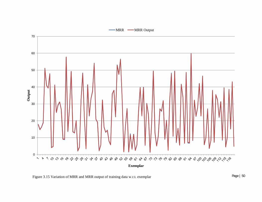
Page | 50

0

10

20

30

40

50

60

70

Out

put

Exemplar

MRR MRR Output

Figure 3.15 Variation of MRR and MRR output of training data w.r.t. exemplar

Page | 51

-0.5

0

0.5

1

1.5

2

1 4 7 10 13 16 19 22 25 28 31 34 37 40 43 46 49 52 55 58 61 64 67 70 73 76 79 82 85 88 91 94 97 100

103

106

109

112

115

118

Out

put

Exemplar

TWR TWR Output

Figure 3.17 Variation of TWR and TWR output of training data set w.r.t exemplar

Page | 52

0

10

20

30

40

50

60

70

1 2 3 4 5 6 7 8 9 10 11 12 13 14 15

Out

put

Exemplar

MRR MRR Output

-0.5

0

0.5

1

1.5

2

1 2 3 4 5 6 7 8 9 10 11 12 13 14 15

Out

put

Exemplar

TWR TWR Output

Figure 3.16 Variation of MRR and MRR output of testing data w.r.t. exemplar

Figure 3.18 Variation of TWR and TWR output of testing data set w.r.t exemplar

Page | 53

3.7 Conclusions

From the main effect plots it can be concluded that for training MSE and R, 32 nos. of hidden

neuron found to give better result but in case of testing MSE and R, 16 nos. of hidden neuron

found to be the best. As training data set is used to fit the model and testing data set is used to

evaluate the model, here main effect plot and ANOVA of testing data set was considered for

evaluation of best ANN model. From ANOVA it can be conclude that nos. of hidden neuron

is having highest contribution towards MSE and R, no matter whether it is for training or

testing. As the neural architecture was found insignificant for test MSE and test R, the

conventional MLP neural architecture was selected for modeling. From the main effect plot

of test MSE and test R, Levenberg-Marquardt training algorithm and 16 nos. of hidden

neurons are found to be efficient for optimal values of responses and hence selected for

efficient ANN modeling and results were demonstrated.

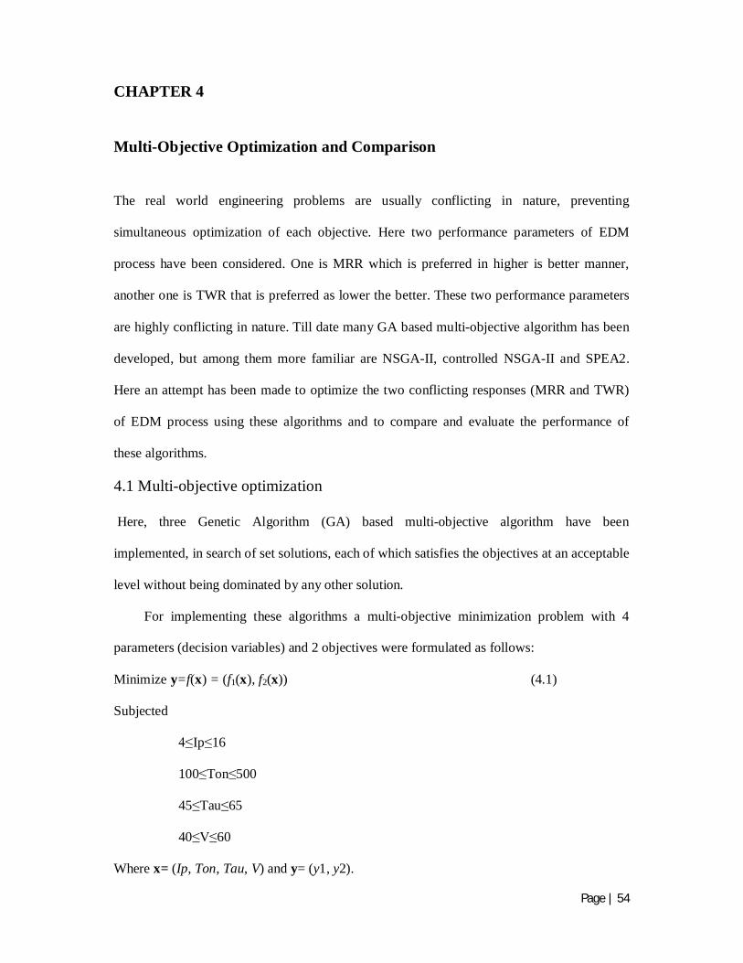
Page | 54

CHAPTER 4

Multi-Objective Optimization and Comparison

The real world engineering problems are usually conflicting in nature, preventing

simultaneous optimization of each objective. Here two performance parameters of EDM

process have been considered. One is MRR which is preferred in higher is better manner,

another one is TWR that is preferred as lower the better. These two performance parameters

are highly conflicting in nature. Till date many GA based multi-objective algorithm has been

developed, but among them more familiar are NSGA-II, controlled NSGA-II and SPEA2.

Here an attempt has been made to optimize the two conflicting responses (MRR and TWR)

of EDM process using these algorithms and to compare and evaluate the performance of

these algorithms.

4.1 Multi-objective optimization

Here, three Genetic Algorithm (GA) based multi-objective algorithm have been

implemented, in search of set solutions, each of which satisfies the objectives at an acceptable

level without being dominated by any other solution.

For implementing these algorithms a multi-objective minimization problem with 4

parameters (decision variables) and 2 objectives were formulated as follows:

Minimize y=f(x) = (f1(x), f2(x)) (4.1)

Subjected

Ip 16

100 Ton 500

45 Tau 65

40 60

Where x= (Ip, Ton, Tau, V) and y= (y1, y2).

Page | 55

The multi-objective function y=f(x) formed by the ANN model equation is to be

minimized but the individual objective MRR is to be maximized and TWR is to be

minimized. So the individual objective MRR was suitably modified. After modification the

individual objective function are represented below as:

( ) =1

1 + (4.2)

( ) (4.3)

4.1.1 Multi-Objective Optimization using NSGA-II

In this algorithm, initially a random initial population Pt of size N is created and for this

generation, the population is sorted based on non-dominance. Then, the binary tournament

selection, reproduction, crossover and mutation operations are performed to create child

population Qt of size N. After the initial generation the procedure changes to preserve the

elitism.

In the subsequent generations, the first step is to combine the child and parent

population. This summed up the total population size to 2N. The combined population Rt

(=Pt+Qt) is sorted on the basis of non-dominance, which generates number of non-dominated

solution fronts. Then, based on crowded comparison criteria, a new parent population Pt+1 of

size N is formed [29]. If any one of the termination criteria met at this stage, then the process

is terminated, otherwise it continues through the steps as shown in Figure 4.1 until the final

state of non-dominated set of solutions are achieved. This algorithm was implemented in

MATLAB code with the functions and parameters setting tabulated in Table 4.1.

Page | 56

Table 4.1 Process parameter and functional setting of NSGA-II algorithm

Types of operation and parameter Functions or parameters value used Population

a. size b. creation function

60 Feasible population

Selection Tournament Reproduction

a. crossover fraction 0.8

Cross over a. crossover function b. crossover ratio

Intermediate 1.0

Mutation Adaptive feasible Distance measure function Distance crowding Stopping criteria

a. generation 800 b. stall generation 100 c. functional tolerance 1x10-6

4.1.2 Multi-Objective Optimization using Controlled NSGA-II

In this algorithm an attempt has been made to form the new parent population Pt+1 of size N

by adding solutions in a predefined distribution manner from each front [30]. The details

about controlled NSGA-II algorithm is shown in Figure 4.2 in the form of a flow chart. All

the functions and parameters setting are same as shown in Table 4.1, except Pareto-front

population fraction (defines the distribution of fit population down to the specified fraction in

order to maintain the diversity) and population size which were set to 0.35 and 171.

4.1.3 Multi-Objective Optimization using SPEA2

SPEA2 algorithm has been presented in the form of flow chart in Figure 4.3. In SPEA2

algorithm for every generation an external set (or external archive) is used to store the newly

formed parent population and the size of the external archive may be different from the initial

population size. The raw fitness assignment of an individual in SPEA2 is decided by strength

of its dominators (in both archive and population) and density (based on kth nearest neighbor

method).The diversity among the solutions is maintained in this algorithm by density

Page | 57

Initialize a random initial population Pt of size N.

Set generation= t=0.

Sort the population on the basis of Non-dominance. Assign a fitness (or rank) to

each solution to its non-domination level.

Perform selection (Use binary tournament selection operator)

Reproduction (Set the crossover fraction)

Perform crossover Perform selection (use crowded

tournament selection operator on Pt+1)

Set t= t+1 Child population Qt of size N is generated.

Combine parent and child population Rt=Pt+Qt

Sort population Rt according to non- dominance. This will generate different non-dominated fronts F1, F2, and so on.

Form a new parent population Pt+1 of size N by adding solutions from first front and

continuing to other fronts successively based on crowded comparison criteria.

Is anyone of the termination criteria met?

Set of decision vectors represented by non-dominated individuals in

Pt+1 are the final solutions.

Stop

Perform mutation

Start

Yes

No

Figure 4.1 Flow chart representation of NSGA-II

Page | 58

Initialize a random initial population Pt of size N.

Set generation= t=0.

Sort the population on the basis of Non-dominance. Assign a fitness (or rank) to

each solution to its non-domination level.

Perform selection (Use binary tournament selection operator)


Perform crossover Perform selection (use crowded

tournament selection operator on Pt+1)

Set t= t+1 Child population Qt of size N is generated.

Combine parent and child population Rt=Pt+Qt

Sort population Rt according to non- dominance. This will generate different non-dominated fronts F1, F2, and so on.

Form a new parent population Pt+1 of size N by adding solutions in a predefined

distribution manner from each front based on crowed comparison criteria.

Is anyone of the termination criteria met?


Pt+1 are the final solutions.

Stop

Perform mutation

Start

Yes

No

Figure 4.2 Flow chart representation of Controlled NSGA-II

Page | 59

estimation (based on kth nearest neighbor method) [31]. For implementing this algorithm, a

MATLAB code was used with initial population size and archive size of 60. Parameters and

functions used for reproduction, crossover and mutation were set as shown in Table 4.1.

4.1.4 Comparison among algorithms

In NSGA-II a new parent population is formed by adding solutions from first front and

continuing to other fronts successively based on crowded comparison criteria till the

population size exceed N. In this process for a particular generation, most of the decision

vectors from combined population (Rt) lie on the non-dominated front of rank one. So almost

all individual of the other front will be deleted to preserve elitism. In this way NSGA-II

ensure diversity along the current non-dominated front. But this leads to loss of lateral

diversity resulting slowdown of search and poor convergence. To avoid this NSGA-II was

slightly modified in the step of formation of a new parent population by adding solutions in a

predefined distribution manner from each front.

If a comparison will be made between NSGA-II and SPEA2 then following outline of

comparison will come out. In case of NSGA-II and controlled NSGA-II, no external

archived is used, but the external set of SPEA2 can be compared with the parent population

of NSGA-II and controlled NSGA-II. In NSGA-II fitness assignment is performed on the

basis of non-dominance and density estimation based on crowding comparison approach.

The diversity among population members of NSGA-II is preserved by crowded comparison

criteria.

.

Page | 60

Start

Calculate fitness values of individuals in Pt and At.

Initialize a random initial population Pt of size N and an empty archive (External set) At of size N. Set

generation = t=0.

Copy all non-dominated individuals in Pt and At to At+1. Maintain the size of At+1 to N (Either using truncation

operator or filling with dominated individuals in Pt and At according to the requirement.)

Is any one of the termination criteria met?


At+1 are the final solutions.

Perform section operation. (Use binary tournament section with

replacement on At+1).


Perform crossover

The resulting population Pt+1 of size N is formed.

Stop

At+1 is the external archive.

Set t=t+1

Perform mutation

Yes

No

Figure 4.3 Flow chart representation of SPEA2 algorithm

Page | 61

4.2 Comparison

The solutions obtained from different algorithms in the form of Pareto-optimal fronts have

been compared on the basis of diversity along the fronts and domination of solutions of one

algorithm over others.

4.2.1. Diversity along the fronts

The diversity is defined by two parameters viz. the optimal length of the Pareto-optimal front

and the pattern of distribution of solutions along the front. In a Pareto-optimal front, for each

individual i the difference between solutions value (distances in objective space) to all

individual j was calculated and was represented by

= + (4.4 )

Where i and j=1, 2, 3…n and n=total nos. of solutions in that Pareto-optimal front,

(xi, yi), (xj, yj) are the simultaneous optimal set of solutions. The dij values for each Pareto-

optimal front were normalized to a common scaling range of 0-1, using min-max data

normalization technique. The superiority can be decided by the maximum length factor (max

(dij)) which is obtained from each algorithm.

However, only the maximum length factor should not be used for evaluating the

superiority of a Pareto-optimal front in terms of diversity because little can be revealed about

the pattern of distribution of solutions from the length factor. For investigating about the

pattern of distribution of solutions, a term cnm is introduced. The better distribution of

solutions were analyzed in both quantitative and qualitative languages. For qualitative

analysis, the histogram plots for corresponds to distance between two consecutive

points/solutions cnm values of Pareto-optimal front of different algorithms were studied.

Where n is any point and m=n+1= 2, 3, 4… N and N=total nos. of solution in a Pareto-

Page | 62

optimal front. Pareto-optimal responses are scaled to individual normalization range of 0-1.

The mean value of cnm for each Pareto-optimal front will be another deciding factor for the

superiority selection. As, Pareto-optimal solutions of each algorithm has been scaled in the

range of 0-1, for better distribution of solutions along each front the average cnm value

should approach to 0.016949153 (=((max (dij) - min (dij)) /(N-1))), which can be coined as

standard mean. So absolute deviations from standard mean (Asd) was also consider to be

another decision making factor for better distribution of solutions along a front. In overall, it

can be said that cnm and Asd were castoff for investigating quantitative study about uniform

distribution of solution along Pareto-optimal front.

4.2.2. Domination of solutions

The domination of non-dominated solutions of one algorithm over another is certainly an

important factor while deciding the superiority of a Pareto-optimal front.

4.3 Results and discussion

4.3.1 Multi-objective optimization

Multi-objective optimization using NSGA-II

Pareto-optimal decision vectors are tabulated in Table 4.2 and plotted as Pareto-optimal front,

which are shown in Figure 4.4. MRR and TWR in Table 4.2 are the neural network predicted

values for corresponding process parameter setting. The solutions denoted by region AB and

CD are responsible for higher MRR with comparison to corresponding TWR. However, the

solutions in the region EF are relatively having higher TWR without much increase in MRR.

Page | 63

Table 4.2 Optimal set of parameters obtained using NAGA-II

S. No.

Ip (A)

Ton (µs) Tau (%) V (volt)

MRR

TWR

1 15.9 497.1 56.3 59.9 41.02 -0.11858 2 16.0 496.0 64.1 41.8 55.33 -0.04952 3 16.0 401.4 64.9 40.3 58.33 0.10790 4 5.4 311.9 57.1 40.6 10.33 -0.12796 5 4.0 309.7 57.8 40.2 5.15 -0.13958 6 15.6 497.2 55.1 59.8 39.10 -0.12210 7 15.7 496.1 63.3 44.2 52.18 -0.06314 8 15.9 496.6 59.6 58.7 43.85 -0.10672 9 16.0 491.9 65.0 41.1 56.47 -0.03977 10 15.4 498.4 54.6 59.9 38.04 -0.12431 11 4.9 312.2 57.8 41.1 8.46 -0.13228 12 15.5 494.9 61.1 56.1 44.74 -0.09685 13 15.9 497.1 56.6 59.8 41.48 -0.11740 14 15.9 497.1 59.3 53.9 45.84 -0.09650 15 16.0 350.6 65.0 40.2 59.15 0.24112 16 15.8 493.2 63.2 44.6 52.79 -0.05916 17 15.9 496.9 61.5 50.5 49.04 -0.08085 18 15.9 432.0 64.9 40.2 57.73 0.04460 19 15.9 497.1 59.5 52.8 46.54 -0.09302 20 15.9 495.7 60.5 43.7 51.61 -0.06704 21 16.0 463.0 64.9 40.2 57.35 -0.00409 22 16.0 376.4 65.0 40.4 58.71 0.16895 23 15.9 495.7 59.3 48.9 48.25 -0.08287 24 16.0 406.4 64.8 40.2 58.15 0.09615 25 16.0 385.1 64.9 40.2 58.58 0.14644 26 15.9 495.9 60.3 48.4 49.11 -0.07946 27 16.0 428.8 65.0 40.2 57.99 0.05204 28 16.0 491.4 64.2 41.0 55.94 -0.04289 29 15.8 498.2 55.6 59.9 40.23 -0.12090 30 16.0 393.2 64.9 40.2 58.50 0.12723 31 16.0 496.6 62.0 41.9 53.62 -0.05900 32 15.9 461.7 64.7 40.2 57.01 -0.00448 33 16.0 362.1 64.9 40.3 58.88 0.20723 34 15.7 494.4 62.6 47.5 50.64 -0.06984 35 4.3 310.9 57.0 40.8 6.19 -0.13703 36 15.8 494.7 59.8 57.6 44.46 -0.10210 37 15.9 496.8 57.9 59.1 42.48 -0.11304 38 14.8 498.4 51.9 60.0 33.69 -0.12599 39 16.0 416.4 65.0 40.2 58.15 0.07615 40 16.0 446.9 65.0 40.2 57.67 0.02040

Page | 64

Figure 4.4 Pareto-optimal front obtained from NSGA-II

-0.2

-0.15

-0.1

-0.05

0

0.05

0.1

0.15

0.2

0.25

0.3

0 10 20 30 40 50 60 70

Tool

Wea

r Rat

e(TW

R)(

mm

3 /min

)

Material Removal Rate (MRR)(mm3/min)

E

F

C

D

BA

41 4.2 309.2 57.0 40.7 5.59 -0.13826 42 16.0 489.4 62.0 41.6 54.04 -0.05092 43 16.0 356.5 64.9 40.2 58.99 0.22318 44 15.0 497.1 55.3 60.0 37.01 -0.12448 45 4.7 310.5 57.1 40.7 7.49 -0.13505 46 5.2 310.2 57.7 40.3 9.69 -0.13038 47 14.8 498.4 51.9 60.0 33.69 -0.12599 48 5.2 310.0 57.1 40.7 9.43 -0.13045 49 4.6 310.6 57.3 40.5 7.09 -0.13609 50 15.8 497.4 54.7 60.0 39.66 -0.12154 51 15.9 494.6 62.1 50.1 49.78 -0.07556 52 15.9 495.1 62.1 53.7 47.91 -0.08441 53 15.4 497.3 55.0 59.9 38.35 -0.12336 54 14.9 497.5 54.2 60.0 35.98 -0.12572 55 16.0 416.4 64.8 40.2 58.10 0.07592 56 16.0 348.8 65.0 40.3 59.17 0.24692 57 16.0 490.5 64.9 40.3 56.92 -0.03670 58 14.9 496.9 53.3 60.0 35.09 -0.12596 59 5.7 312.6 57.1 40.1 11.19 -0.12608 60 16.0 372.2 65.0 40.3 58.82 0.18013

Page | 65

Multi-Objective Optimization using Controlled NSGA-II

A set of Pareto-optimal solutions obtained using controlled NSGA-II is shown in Figure

4.5 in the form of Pareto-optimal front and the same are tabulated in Table 4.3. Here also the

effect of various regions AB, CD and EF of Pareto-optimal front have approximately same

effect on the optimal responses MRR and TWR as in NSGA-II. But in NSGA-II the

maximum value of TWR that can be achieved with its optimal process parameter setting was

up to 0.241 (mm3/min) meanwhile in controlled NSGA-II it was extended up to 1.343

(mm3/min). This indicates that controlled NSGA-II expanded the band of optimal process

parameter setting.

Table 4.3 Optimal sets of parameters obtained using Controlled NAGA-II

S. No. Ip (A)

Ton (µs)

Tau (%)

V (volt)

MRR

TWR

1 5.8 331.0 59.9 40.2 11.87 -0.12389 2 15.9 489.9 62.8 41.9 54.23 -0.05032 3 15.9 473.7 64.4 42.3 55.33 -0.02756 4 4.9 312.9 59.8 40.2 8.37 -0.13235 5 5.8 331.0 59.9 40.2 11.87 -0.12389 6 16.0 331.7 65.0 40.1 59.50 0.30093 7 16.0 124.9 65.0 40.0 61.28 1.26833 8 16.0 213.3 65.0 40.0 60.73 0.78189 9 16.0 426.5 65.0 40.2 58.06 0.05674 10 16.0 349.8 65.0 40.2 59.21 0.24432 11 16.0 193.3 65.0 40.1 60.82 0.88173 12 16.0 479.1 64.9 40.5 56.95 -0.02517 13 15.6 490.9 62.0 43.1 51.65 -0.06224 14 16.0 378.3 65.0 40.2 58.81 0.16509 15 15.1 489.4 58.7 55.4 41.87 -0.10343 16 14.7 492.1 57.3 57.9 38.34 -0.11537 17 4.2 303.3 59.4 40.2 6.05 -0.13858 18 15.4 491.8 57.5 57.7 41.18 -0.11068 19 16.0 112.8 65.0 40.0 61.34 1.34351 20 16.0 233.2 65.0 40.2 60.49 0.68635 21 15.5 491.5 61.0 44.8 49.51 -0.07187 22 16.0 154.0 65.0 40.0 61.12 1.09608 23 5.5 325.2 59.4 40.2 10.61 -0.12732 24 14.5 491.5 54.6 59.3 35.04 -0.12239

Page | 66

25 15.4 485.3 59.5 40.2 50.08 -0.06225 26 15.8 490.6 60.9 56.0 45.77 -0.09199 27 16.0 124.9 65.0 40.0 61.28 1.26835 28 16.0 112.8 65.0 40.0 61.34 1.34354 29 15.8 491.2 60.2 57.2 44.69 -0.09803 30 15.4 489.8 55.7 58.2 39.68 -0.11405 31 15.9 473.7 64.4 42.3 55.31 -0.02766 32 16.0 367.5 65.0 40.2 59.00 0.19402 33 4.8 307.7 59.6 40.2 7.99 -0.13380 34 15.5 490.4 60.6 50.7 46.94 -0.08391 35 16.0 308.8 65.0 40.3 59.67 0.37760 36 5.2 323.5 59.9 40.2 9.31 -0.12941 37 15.6 486.8 58.1 55.5 43.36 -0.09874 38 15.6 489.2 63.7 43.3 52.61 -0.05532 39 15.9 488.9 57.5 56.9 43.31 -0.10230 40 16.0 184.5 64.9 40.1 60.88 0.92792 41 16.0 294.1 65.0 40.1 59.95 0.43256 42 16.0 404.6 65.0 40.2 58.44 0.10215 43 16.0 282.1 65.0 40.1 60.08 0.47841 44 15.3 490.8 59.9 44.2 48.24 -0.07554 45 16.0 164.4 65.0 40.0 61.08 1.03764 46 16.0 174.7 65.0 40.0 61.00 0.98075 47 16.0 203.1 65.0 40.1 60.79 0.83217 48 16.0 218.3 65.0 40.1 60.65 0.75711 49 16.0 249.3 65.0 40.1 60.41 0.61503 50 16.0 442.1 64.9 40.3 57.60 0.02726 51 16.0 320.8 65.0 40.1 59.61 0.33695 52 16.0 151.1 65.0 40.1 61.13 1.11252 53 14.4 492.5 53.4 59.6 33.85 -0.12389 54 16.0 450.2 64.9 40.6 57.36 0.01373 55 14.9 492.2 54.7 58.9 36.92 -0.12080 56 16.0 134.6 65.0 40.0 61.22 1.20951 57 15.0 492.4 58.5 58.3 39.79 -0.11271 58 16.0 143.5 65.0 40.0 61.20 1.15693 59 16.0 134.6 65.0 40.0 61.21 1.20935 60 14.7 492.1 57.3 57.9 38.34 -0.11536

Page | 67

Figure 4.5 Pareto-optimal front obtained from Controlled NSGA-II

Multi-Objective Optimization using SPEA2

Final non-dominated set of solutions are tabulated in Table 4.4 and has been represented in

the form of graph in Figure 4.6. The non-dominated decision vectors of region AB and CD of

the Pareto-optimal front of SPEA2 algorithm will generate more MRR as compared to

respective TWR. And final non-dominated solutions corresponding to region DE will act in

the reverse manner as that of region AB and CD.

Table 4.4 Optimal sets of parameters obtained using SPEA2

S. No. Ip (A)

Ton (µs)

Tau (%)

V (volt)

MRR

TWR

1 16.0 498.8 64.9 40.2 56.88 -0.04415 2 16.0 499.9 61.9 40.8 54.30 -0.05853 3 16.0 472.2 64.8 40.0 57.30 -0.01585 4 5.2 319.8 59.2 40.0 9.42 -0.13073 5 16.0 500.0 61.3 58.6 45.50 -0.10107 6 4.3 293.9 57.8 40.0 6.52 -0.13949 7 16.0 500.0 58.9 59.8 43.30 -0.11300 8 5.7 322.8 58.1 40.0 11.21 -0.12705 9 15.2 500.0 53.3 60.0 36.10 -0.12669

-0.4

-0.2

0

0.2

0.4

0.6

0.8

1

1.2

1.4

1.6

0 10 20 30 40 50 60 70

Tool

Wea

r Rat

e (T

WR)

(mm

3/m

in)

Material Removal Rate (MRR) (mm3/min)

A B C D

E

Page | 68

S. No. Ip (A)

Ton (µs)

Tau (%)

V (volt)

MRR

TWR

10 15.0 500.0 53.0 60.0 35.47 -0.12687 11 15.0 500.0 54.6 60.0 36.53 -0.12623 12 16.0 500.0 56.7 59.9 41.63 -0.11908 13 14.9 500.0 52.9 60.0 34.93 -0.12692 14 15.9 500.0 61.1 55.9 46.41 -0.09635 15 4.5 297.6 58.9 40.0 7.12 -0.13723 16 16.0 500.0 65.0 41.4 56.28 -0.04745 17 16.0 500.0 60.6 54.5 46.93 -0.09451 18 16.0 319.9 65.0 40.1 59.68 0.34041 19 16.0 100.3 65.0 40.0 61.40 1.42315 20 16.0 417.8 64.9 40.1 58.25 0.07438 21 16.0 500.0 60.6 52.0 48.08 -0.08866 22 16.0 500.0 57.7 58.7 42.87 -0.11378 23 16.0 499.0 61.1 50.1 49.31 -0.08191 24 15.2 500.0 54.3 59.9 36.99 -0.12606 25 16.0 355.7 65.0 40.1 59.23 0.22767 26 16.0 500.0 61.1 59.7 44.92 -0.10451 27 16.0 293.1 65.0 40.0 60.03 0.43685 28 16.0 500.0 55.4 60.0 40.49 -0.12175 29 16.0 500.0 61.4 57.8 45.96 -0.09894 30 5.0 298.2 57.8 40.0 8.84 -0.13241 31 16.0 187.8 64.9 40.0 60.90 0.91101 32 16.0 498.2 61.0 40.4 53.70 -0.05931 33 15.5 500.0 54.1 60.0 37.81 -0.12554 34 16.0 500.0 60.4 59.8 44.33 -0.10759 35 15.6 500.0 54.4 59.9 38.55 -0.12461 36 4.7 314.3 57.3 40.5 7.70 -0.13455 37 16.0 500.0 60.5 50.3 48.77 -0.08516 38 4.2 289.2 56.8 40.1 6.00 -0.14077 39 16.0 499.8 60.5 46.5 50.56 -0.07588 40 16.0 499.2 62.0 50.1 49.98 -0.07856 41 16.0 500.0 55.9 59.9 41.10 -0.12046 42 15.6 500.0 55.6 59.9 39.46 -0.12323 43 5.5 307.7 58.0 40.1 10.65 -0.12731 44 16.0 500.0 63.3 46.6 52.57 -0.06598 45 16.0 500.0 62.6 48.7 51.13 -0.07330 46 16.0 399.2 65.0 40.0 58.64 0.11501 47 16.0 500.0 60.3 52.7 47.54 -0.09127 48 4.0 288.8 57.5 40.0 5.38 -0.14282 49 16.0 500.0 59.4 59.6 43.81 -0.11068 50 16.0 249.4 65.0 40.0 60.46 0.61477 51 16.0 500.0 63.1 41.5 54.87 -0.05589

Page | 69

S. No. Ip (A)

Ton (µs)

Tau (%)

V (volt)

MRR

TWR

52 4.9 309.9 57.1 40.0 8.29 -0.13446 53 16.0 430.7 64.5 40.1 57.74 0.04724 54 16.0 499.8 63.2 40.8 55.23 -0.05411 55 5.3 311.8 58.6 40.0 10.00 -0.12970 56 16.0 499.9 62.5 46.8 51.94 -0.06953 57 16.0 500.0 54.7 60.0 40.10 -0.12232 58 16.0 500.0 62.6 44.4 53.11 -0.06419 59 16.0 500.0 57.6 60.0 42.34 -0.11702 60 16.0 499.9 63.5 40.7 55.58 -0.05232

Figure 4.6 Pareto-optimal front obtained from SPEA2

4.3.2 Comparison

Pareto-optimal front obtained from these three algorithms have been shown in Figure 4.7 for

comparison purpose.

-0.4

-0.2

0

0.2

0.4

0.6

0.8

1

1.2

1.4

1.6

0 10 20 30 40 50 60 70

Tool

Wea

r Rat

e (T

WR

) (m

m3/

min

)

Material Removal Rate (MRR) (mm3/min)

A B C D

E

Page | 70

Figure 4.7 Pareto-optimal fronts of different Algorithms

Diversity along the fronts:

The maximum length factor (for all i belongs to1, 2, 3…, n) has been tabulated in Table 4.5.

Table 4.5 Maximum length factor values

Optimization Algorithm maximum length factor, (max(dij)) ) value

NSGA-II 0.9915

CNSGA-II 1.3645

SPEA2 1.4113

From Table 4.5, it can be conclude that Pareto-optimal front obtained from SPEA2 is

having maximum length factor as compared to other two, and front obtained from NSGA-II

is having lowest span length.

A qualitative analysis on distribution of solutions along the Pareto optimal front can be

performed using histogram plot of normalized cnm values of different algorithms as shown in

Figure 4.8-4.10. The cnm for NSGA-II is having an exponential distribution with an outiler

-0.4

-0.2

0

0.2

0.4

0.6

0.8

1

1.2

1.4

1.6

0 10 20 30 40 50 60 70

Tool

Wea

r Rat

e(m

m3 /m

in)

Material Removal Rate(mm3/min)

CNSGA-II

NSGA-II

SPEA2

Page | 71

(cnm = 0.4) on the extreme right side of Fig. 4.8. The same for CNSGA-II is having a

uniform distribution between 0.0 to 0.1 and with an outlier at 0.4 (Figure 4.9). The

distribution for SPEA2 is having exponential nature as shown in Figure 4.10; with three

solutions are having much higher cnm values in comparison with the rest of distribution. The

histogram plots do not reveal any quantitative analysis, so for better understanding of the

distributions, the quantitative analysis has been followed up next. The normalized mean

distances between two consecutive points/solutions (cnm) and absolute deviations from

standard mean in the Pareto-optimal front of different algorithms have been tabulated below

in Table 4.6.

The lower average value of cnm and Asd indicates better distribution of solutions along

the front. The normalized average value of cnm and Asd in Table 4.6 indicates that the solutions

of Pareto-optimal front obtained from NSGA-II are distributed in a better manner as

compared to the solutions of the other two algorithms. Pareto-optimal front obtained from

SPEA2 is having poor distribution of solution along the front.

Domination of solutions:

The domination of non-dominated solutions of one algorithm over another has been shown

in Table 4.7 in a comparative manner. It shows that non-dominated solution set achieved by

NSGA –II dominates about 53% and 5% of the non-dominated solutions found by CNSGA-II

and SPEA2, respectively. CNSGA-II dominates about 13% of the non-dominated solutions of

Pareto-optimal front obtained from NSGA-II. the SPEA2 Pareto-optimal front dominates on

an average 85% and 100% of the solutions of NSGA-II and CNSGA-II, respectively.

The SPEA2 algorithm is generating a superior optimal set of solutions based on the

domination of solutions and the length of the Pareto-optimal front.

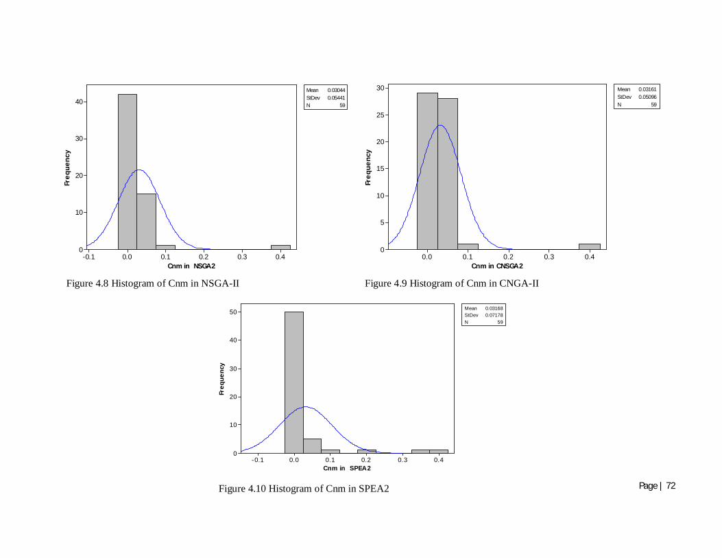
Page | 72

0.40.30.20.10.0-0.1

40

30

20

10

0

Cnm in NSGA2

Freq

uenc

y

Mean 0.03044StDev 0.05441N 59

0.40.30.20.10.0

30

25

20

15

10

5

0

Cnm in CNSGA2

Freq

uenc

y

Mean 0.03161StDev 0.05096N 59

0.40.30.20.10.0-0.1

50

40

30

20

10

0

Cnm in SPEA2

Freq

uenc

y

Mean 0.03168StDev 0.07178N 59

Figure 4.10 Histogram of Cnm in SPEA2

Figure 4.8 Histogram of Cnm in NSGA-II Figure 4.9 Histogram of Cnm in CNGA-II

Page | 73

Table 4.6 Mean of normalized cnm values

Optimization

Algorithm Mean normalized cnm value Absolute deviations from

standard mean (Asd)

NSGA-II 0.030438 0.013489

CNSGA-II 0.031606 0.014657

SPEA2 0.031679 0.01473

Table 4.7 Domination of percentage of solutions

Algorithm dominates “non-dominated solutions” found by

NSGA-II with a

percentage of

CNSGA-II with a

percentage of

SPEA2 with a

percentage of

NSGA-II ------------------------ 53% 5%

CNSGA-II 13% -------------------------- 0%

SPEA2 85% 100% --------------------------

4.3.3 Post-optimality analysis of Pareto-optimal solutions

The post-optimality analysis of SPEA2 Pareto-optimal front has been performed in this

section. This analysis is mainly concerned with whether the optimal set of solution is affected

by optimal setting of the machining parameters or not. The individual effect of optimal

process parameters Ip, Ton, Tau and V on MRR has been represented in Figure 4.11.

Similarly, the effects on TWR have been plotted in Figure 4.12. From Figure 4.11, it can be

observed that the maximum MRR is achieved for the parameters setting Ip and Tau towards

their upper bounds and the parameters Ton and V towards their lower bounds. Similarly,

from Figure 4.12, it can be conclude that the optimum TWR can be achieved by the

parameters setting of Ip and Tau towards their lower bounds, V towards its upper bound, and

Ton in the middle of the machining range.

Page | 74

Figure 4.11 Effect of optimal process parameters on optimal MRR

0100200300400500600

0 10 20 30 40 50 60 70

Ton

(µs)

MRR (mm3/min)

Series1

0

20

40

60

80

0 10 20 30 40 50 60 70

Volta

ge (V

)

MRR(mm3/min)

010203040506070

0 10 20 30 40 50 60 70

Tau

(%)

MRR (mm3/min)

0

5

10

15

20

0 10 20 30 40 50 60 70

Ip (A

)

MRR (mm3/min)

Page | 75

Figure 4.12 Effect of optimal process parameters on optimal TWR

0100200300400500600

-0.4 -0.2 0 0.2 0.4 0.6 0.8 1 1.2 1.4 1.6

Ton(

µs)

TWR(mm3/min)

0

20

40

60

80

-0.4 -0.2 0 0.2 0.4 0.6 0.8 1 1.2 1.4 1.6

Tau(

%)

TWR(mm3/min)

010203040506070

-0.4 -0.2 0 0.2 0.4 0.6 0.8 1 1.2 1.4 1.6

Volta

ge(V

)

TWR(mm3/min)

0

5

10

15

20

-0.4 -0.2 0 0.2 0.4 0.6 0.8 1 1.2 1.4 1.6

Ip(A

)

TWR(mm3/min)

Page | 76

4.4 Conclusions:

Three widely used MOEAs, namely, NSGA-II, CNSGA-II and SPEA2 were successfully

implemented for MOO of responses MRR and TWR of EDM process. From each algorithm,

the Pareto-optimal front consisting of 60 optimal set of solutions was obtained with their

process parameter setting. A comparison was made between the solutions of these three

algorithms to find out the best among them. The comparison was made based on two basic

parameters, the diversity along the fronts in terms of maximum Pareto-optimal front span and

better distribution of solutions, and the domination of solutions of one algorithm over

another. SPEA2 outperformed the other two algorithms on the basis of domination of

solutions. However, NSGA-II was found to be the best while consideration of better

distribution of solutions. Finally, a post-optimality analysis was performed, which showed the

effect of optimal process parameters on optimal responses MRR and TWR for SPEA2.

Page | 77

CHAPTER 5

Concluding Remarks

The primary objective of this investigation was to develop an optimal ANN modeling (as

modelling save the time, effort and money) and to optimize the two contradicting responses

MRR and TWR of EDM process using reliable and efficient MOEAs.

An efficient modeling of EDM response parameters MRR and TWR was successfully

executed. The modelling was accomplished using MLP neural architecture with 16 hidden

layer neurons, trained by Levenberg-Marquardt algorithm. The ANOVA revealed that

number of hidden layer neurons has highest significance towards the performance of an ANN

modeling, and followed by the learning algorithm.

Each of the three MOEAs (NSGA-II, CNSGA-II and SPEA2) has fruitfully generated a set of

60 optimal solutions. The optimal solutions generated by SPEA2 was found to be superlative

compare to the same by the other two algorithms for this particular assigned task.

Page | 78

APPENDIX A

Levenberg-Marquardt Training/Learning Algorithm

Below an attempt has been made to give shape to Levenberg-Marquardt optimization

(minimization) technique so that it can be used for training ANN (to update the weight matrix of

output layer and one hidden layer respectively in batch mode of training) using cross-validation

as stopping criteria (in every100 epochs):

Levenberg-Marquardt algorithm:

Step 1:

Define and

(Here the weight matrixes are decided by random weight initialization technique.)

M = maximum number of iterations allowed

m=running iteration number

Step 2:

Set m=0, = 10

Find ( ) and( )

Step 3:

Is %100 0?

Yes: Then set = ( )

Check, is … … … … … … < ?

Yes: Go to step 12.

No: continue

No: continue

Page | 79

Step 4:

Is m M?

Yes: Go to step 12.

No: continue

Step 5:

Calculate and .

Step 6:

Calculate ]

and ]

Step 7:

Set

and

Step 8:

Find ( ) and( )

Step 9:

Is( ) < ( ) ?

Yes: Go to step 10.

No: Go to step 11.

Step 10:

Set = and set m=m+1.Go to step 3.

Step 11:

Set = 10 .Go to step 6.

Page | 80

Step 12:

Stop the training and print the result at the minimum of the validation set error.

Where,

weights are connection strengths between hidden and output layer. Weights are

connection strengths between input and hidden layer. Where k and j indicates the neuron number

of output and hidden layer respectively and i indicate input unit number.

( ) and ( ) are the mean squared error of training data set and cross-validation data set

respectively at iteration m.

is Jacobian matrix of average mean squared error function w.r.t. weights .

is Jacobian matrix of average mean squared error function w.r.t. weights .

and are the Hessian matrix.

Here and are the identity matrix, that is, it contains zeros except for the diagonal

elements, which are +1.

and are the search directions.

In the similar manner the biases of an ANN can also be optimized to achieve minimum MSE.

Page | 81

BIBLIOGRAPHY:

1. Elman C. Jameson, Electrical Discharge Machining, Society of Manufacturing Engineers (2001), p.1.

2. K.H. Ho, S.T. Newman, State of the art electrical discharge machining (EDM), International Journal of Machine Tools & Manufacture (2003), 43, 1287–1300.

3. Antoine Descoeudres, Characterization of electrical discharge machining plasmas, Ph.D. Thesis (2006), School Polytechnique Federale de Lausanne, Thèse EPFL, no 3542.

4. Kuo-Ming Tsai, Pei-Jen Wang, Comparison of neural network models on material removal rate in electric discharge machining, Journal of Materials Processing Technology (2001), 117,111-124.

5. H. Juhr, K. Künanz, A. Nestler, G. Leitte, Generation of parameter technologies for EDM die sinking with artificial neural networks (ANN) and nonlinear regression functions (NRF), Forschungsergebnis bericht, 2004.

6. Deepak Kumar Panda, Rajat Kumar Bhoi, Artificial Neural Network Prediction of Material Removal Rate in Electro Discharge Machining, Materials and Manufacturing Processes (2005), 20: 4, 645 — 672.

7. Angelos P. Markopoulos,Dimitrios E. Manolakos, Nikolaos M. Vaxevanidis, Artificial neural network models for the prediction of surface roughness in electrical discharge machining, J Intell Manuf (2008), 19:283–292.

8. S. Assarzadeh & M. Ghoreishi, Neural-network-based modeling and optimization of the electro-discharge machining process, Int J Adv Manuf Technol (2008), 39:488–500.

9. S. N. Joshi & S. S. Pande, Development of an intelligent process model for EDM, Int J Adv Manuf Technol (2009), 45:300–317.

10. M K Pradhan, R Das, and C K Biswas, Comparisons of neural network models on surface roughness in electrical discharge machining, J. Engineering Manufacture (2009), Vol. 223, Part B, 801-808.

11. Promod Kumar Patowari & Partha Saha & P. K. Mishra, Artificial neural network model in surface modification by EDM using tungsten–copper powder metallurgy sintered electrodes, Int J Adv Manuf Technol (2010), 51:627–638.

Page | 82

12. Md. Ashikur Rahman Khan, M. M. Rahman, K. Kadirgama, M.A. Maleque and Rosli A. Bakar, Artificial Intelligence Model to Predict Surface Roughness of Ti-15-3 Alloy in EDM Process, World Academy of Science, Engineering and Technology (2011), 74.

13. Pushpendra S. Bharti, S. Maheshwari, C. Sharma, A comparative study of Artificial Neural Network training algorithms for modeling of Electric Discharge Machining process, Strojnicka Casopis( 2010), 61, c. 5-6.

14. M K Pradhan, R Das, Recurrent neural network estimation of material removal rate in electrical discharge machining of AISI D2 tool steel, Proc. IMechE (2010), Vol. 225 Part B: J.Engineering Manufacturing.

15. A.Thillaivanan, P. Asokan, K.N.Srinivasan, R.Saravanan, Optimization of operating parameters for EDM process based on the Taguchi Method and Artificial Neural Network, International Journal of Engineering Science and Technology (2010), Vol. 2(12), 6880-6888.

16. Cao Fenggou,Yang Dayong, The study of high efficiency and intelligent optimization system in EDM sinking process, Journal of Materials Processing Technology (2004), 149 83–87.

17. G. Krishna Mohana Rao and D. Hanumantha Rao, Hybrid modeling and optimization of hardness of surface produced by electric discharge machining using artificial neural networks and genetic algorithm, Asian Research Publishing Network (ARPN) ( 2010), Vol. 5, No. 5, 72-81.

18. Deepak Kumar Panda, Modelling and Optimization of Multiple Process Attributes of Electro discharge Machining Process by Using a New Hybrid Approach of Neuro-Grey Modeling, Materials and Manufacturing Processes(2010), 25: 6, 450 — 461.

19. Mohan Kumar Pradhan, Chandan Kumar Biswas, Neuro-fuzzy and neural network-based prediction of various responses in electrical discharge machining of AISI D2 steel, Int J Adv Manuf Technol (2010), 50:591–610.

20. Shyam P. Kodali, Rajesh Kudikala and K. Deb, Multi-Objective Optimization of Surface Grinding Process Using NSGA II, First International Conference on Emerging Trends in Engineering and Technology(2008), IEEE.

21. Kesheng Wang, Hirpa L. Gelgele, Yi Wang, Qingfeng Yuan, Minglung Fang, A hybrid intelligent method for modelling the EDM process, International Journal of Machine Tools & Manufacture (2003), 43, 995–999.

Page | 83

22. J. C. Su , J. Y. Kao , Y. S. Tarng, Optimisation of the electrical discharge machining

process using a GA-based neural network , Int J Adv Manuf Technol (2004) 24: 81–90.

23. S.N. Joshi, S.S. Pande, Intelligent process modeling and optimization of die-sinking electric discharge machining, Applied Soft Computing (2011), 11, 2743–2755.

24. Debabrata Mandal, Surjya K. Pal , Partha Saha, Modeling of electrical discharge machining process using back propagation neural network and multi-objective optimization using non-dominating sorting genetic algorithm-II, Journal of Materials Processing Technology (2007), 186,154–162.

25. Shajan Kuriakose and M.S. Shunmugam, Multi-objective optimization of wire-electro

discharge machining process by Non-Dominated Sorting Genetic Algorithm, Journal of Materials Processing Technology (2005), 170, 133–141.

26. Nixon Kuruvila and H. V. Ravindra, Parametric influence and optimization of wire EDM of hot die steel, Machining Science and Technology (2011), 15:47–7.

27. Ramezan Ali MahdaviNejad, Modeling and Optimization of Electrical Discharge Machining of SiC Parameters, Using Neural Network and Non-dominating Sorting Genetic Algorithm (NSGA II), Materials Sciences and Applications (2011), 2, 669-675.

28. Mohan Kumar Pradhan, Experimental Investigation and Modelling of Surface Integrity, Accuracy and Productivity Aspects in EDM of AISI D2 Steel, PhD Dissertation(2010), National Institute of Technology, Rourkela,pp.158-164.

29. Kalyanmoy Deb, Amrit Pratap, Sameer Agarwal, and T. Meyarivan, A Fast and Elitist Multiobjective Genetic Algorithm: NSGA-II, IEEE transactions on Evolutionary Computation (2002), Vol. 6, No. 2,182-197.

30. Kalyanmoy Deb and Tushar Goel, Controlled Elitist Non-dominated Sorting Genetic Algorithms for Better Convergence, Evolutionary Multi-Criterion Optimization, Lecture Notes in Computer Science (2001), Volume 1993/2001, 67-81,

31. E. Zitzler, M. Laumanns, and L. Thiele. SPEA2: Improving the Strength Pareto Evolutionary Algorithm. Technical report 103, Computer Engineering and Networks Laboratory (TIK), ETH Zurich, Zurich, Switzerland, 2001.

Neural Network Modelling and Multi-Objective Optimization...

Documents

Transcript of Neural Network Modelling and Multi-Objective Optimization...