Neural Models for Information Retrieval

Bhaskar MitraMicrosoft, UCL∗Cambridge, UK

bmitra@microsoft.com

Nick CraswellMicrosoft

Bellevue, USAnickcr@microsoft.com

Abstract

Neural ranking models for information retrieval (IR) use shallow or deep neuralnetworks to rank search results in response to a query. Traditional learning torank models employ machine learning techniques over hand-crafted IR features.By contrast, neural models learn representations of language from raw text thatcan bridge the gap between query and document vocabulary. Unlike classical IRmodels, these new machine learning based approaches are data-hungry, requiringlarge scale training data before they can be deployed. This tutorial introduces basicconcepts and intuitions behind neural IR models, and places them in the context oftraditional retrieval models. We begin by introducing fundamental concepts of IRand different neural and non-neural approaches to learning vector representationsof text. We then review shallow neural IR methods that employ pre-trained neuralterm embeddings without learning the IR task end-to-end. We introduce deepneural networks next, discussing popular deep architectures. Finally, we review thecurrent DNN models for information retrieval. We conclude with a discussion onpotential future directions for neural IR.

1 Introduction

Since the turn of the decade, there have been dramatic improvements in performance in computervision, speech recognition, and machine translation tasks, witnessed in research and in real-worldapplications [112]. These breakthroughs were largely fuelled by recent advances in neural networkmodels, usually with multiple hidden layers, known as deep architectures [8, 49, 81, 103, 112].Exciting novel applications, such as conversational agents [185, 203], have also emerged, as wellas game-playing agents with human-level performance [147, 180]. Work has now begun in theinformation retrieval (IR) community to apply these neural methods, leading to the possibility ofadvancing the state of the art or even achieving breakthrough performance as in these other fields.

Retrieval of information can take many forms. Users can express their information need in the form ofa text query—by typing on a keyboard, by selecting a query suggestion, or by voice recognition—orthe query can be in the form of an image, or in some cases the need can even be implicit. Retrieval caninvolve ranking existing pieces of content, such as documents or short-text answers, or composingnew responses incorporating retrieved information. Both the information need and the retrievedresults may use the same modality (e.g., retrieving text documents in response to keyword queries),or different ones (e.g., image search using text queries). Retrieval systems may consider user history,physical location, temporal changes in information, or other context when ranking results. They mayalso help users formulate their intent (e.g., via query auto-completion or query suggestion) and/orextract succinct summaries of results for easier inspection.

Neural IR refers to the application of shallow or deep neural networks to these retrieval tasks. Thistutorial serves as an introduction to neural methods for ranking documents in response to a query, an

∗The author is a part-time PhD student at University College London.

DRAFT. Copyright is held by the author(s). May, 2017.

arX

iv:1

705.

0150

9v1

[cs

.IR

] 3

May

201

7

2014 2015 2016 2017

1 %

4 %

8 %

21 %

05

10

15

20

25

30

Year

% o

f S

IGIR

pa

pe

rs

rela

ted

to

ne

ura

l IR

Figure 1: The percentage of neural IR papers at the ACM SIGIR conference—as determined by amanual inspection of the paper titles—shows a clear trend in the growing popularity of the field.

important IR task. A search query may typically contain a few terms, while the document length,depending on the scenario, may range from a few terms to hundreds of sentences or more. Neuralmodels for IR use vector representations of text, and usually contain a large number of parametersthat needs to be tuned. ML models with large set of parameters typically require a large quantityof training data [196]. Unlike traditional learning to rank (L2R) approaches that train ML modelsover a set of hand-crafted features, neural models for IR typically accept the raw text of a query anddocument as input. Learning suitable representations of text also demands large-scale datasets fortraining [141]. Therefore, unlike classical IR models, these neural approaches tend to be data-hungry,with performance that improves with more training data.

Text representations can be learnt in an unsupervised or supervised fashion. The supervised approachuses IR data such as labeled query-document pairs, to learn a representation that is optimized end-to-end for the task at hand. If sufficient IR labels are not available, the unsupervised approach learnsa representation using just the queries and/or documents. In the latter case, different unsupervisedlearning setups may lead to different vector representations, that differ in the notion of similaritythat they capture between represented items. When applying such representations, the choice ofunsupervised learning setup should be carefully considered, to yield a notion of text similarity thatis suitable for the target task. Traditional IR models such as Latent Semantic Analysis (LSA) [48]learn dense vector representations of terms and documents. Neural representation learning modelsshare some commonalities with these traditional approaches. Much of our understanding of thesetraditional approaches from decades of research can be extended to these modern representationlearning models.

In other fields, advances in neural networks have been fuelled by specific datasets and applicationneeds. For example, the datasets and successful architectures are quite different in visual objectrecognition, speech recognition, and game playing agents. While IR shares some common attributeswith the field of natural language processing, it also comes with its own set of unique challenges.IR systems must deal with short queries that may contain previously unseen vocabulary, to matchagainst documents that vary in length, to find relevant documents that may also contain large sectionsof irrelevant text. IR systems should learn patterns in query and document text that indicate relevance,even if query and document use different vocabulary, and even if the patterns are task-specific orcontext-specific.

The goal of this tutorial is to introduce the fundamentals of neural IR, in context of traditional IRresearch, with visual examples to illustrate key concepts and a consistent mathematical notation fordescribing key models. Section 2 presents a survey of IR tasks, challenges, metrics and non-neuralmodels. Section 3 provides a brief overview of neural IR models and a taxonomy for different neuralapproaches to IR. Section 4 introduces neural and non-neural methods for learning term embeddings,without the use of supervision from IR labels, and with a focus on the notion of similarity. Section 5surveys some specific approaches for incorporating such embeddings in IR. Section 6 introduces thefundamentals of deep models that are used in IR so far, including popular architectures and toolkits.

2

Section 7 surveys some specific approaches for incorporating deep neural networks in IR. Section 8is our discussion, including future work, and conclusion.

Motivation for this tutorial Neural IR is an emerging field. Research publication in the area hasbeen increasing (Figure 1), along with relevant workshops [42–44], tutorials [97, 119, 140], andplenary talks [41, 129]. Because this growth in interest is fairly recent, some researchers with IRexpertise may be unfamiliar with neural models, and other researchers who have already workedwith neural models may be unfamiliar with IR. The purpose of this tutorial is to bridge the gap, bydescribing the relevant IR concepts and neural methods in the current literature.

2 Fundamentals of text retrieval

We focus on text retrieval in IR, where the user enters a text query and the system returns a rankedlist of search results. Search results may be passages of text or full text documents. The system’sgoal is to rank the user’s preferred search results at the top. This problem is a central one in the IRliterature, with well understood challenges and solutions. This section provides an overview of those,such that we can refer to them in subsequent sections.

2.1 IR tasks

Text retrieval methods for full text documents and for short text passages have application in ad hocretrieval systems and question answering systems respectively.

Ad-hoc retrieval Ranked document retrieval is a classic problem in information retrieval, as in themain task of the Text Retrieval Conference [205], and performed by popular search engines suchas Google, Bing, Baidu, or Yandex. TREC tasks may offer a choice of query length, ranging froma few words to a few sentences, whereas search engine queries tend to be at the shorter end of therange. In an operational search engine, the retrieval system uses specialized index structures to searchpotentially billions of documents. The results ranking is presented in a search engine results page(SERP), with each result appearing as a summary and a hyperlink. The engine can instrument theSERP, gathering implicit feedback on the quality of search results such as click decisions and dwelltimes.

A ranking model can take a variety of input features. Some ranking features may depend on thedocument alone, such as how popular the document is with users, how many incoming links it has,or to what extent document seems problematic according to a Web spam classifier. Other featuresdepend on how the query matches the text content of the document. Still more features match thequery against document metadata, such as referred text of incoming hyperlink anchors, or the text ofqueries from previous users that led to clicks on this document. Because anchors and click queriesare a succinct description of the document, they can be a useful source of ranking evidence, but theyare not always available. A newly created document would not have much link or click text. Also,not every document is popular enough to have past links and clicks, but it still may be the best searchresult for a user’s rare or tail query. In such cases, when text metadata is unavailable, it is crucial toestimate the document’s relevance primarily based on its text content.

In the text retrieval community, retrieving documents for short-text queries by considering the longbody text of the document is an important challenge. The ad-hoc and Web tracks2 at the popularText REtrieval Conference (TREC) [204] focus specifically on this task. The TREC participants areprovided a set of, say fifty, search queries and a document collection containing 500-700K newswireand other documents. Top ranked documents retrieved for each query from the collection by differentcompeting retrieval systems are assessed by human annotators based on their relevance to the query.Given a query, the goal of the IR model is to rank documents with better assessor ratings higherthan the rest of the documents in the collection. In Section 2.4, we describe popular IR metricsfor quantifying model performance given the ranked documents retrieved by the model and thecorresponding assessor judgments for a given query.

Question-answering Question-answering tasks may range from choosing between multiple choices(typically entities or binary true-or-false decisions) [78, 80, 165, 212] to ranking spans of text or

2http://www10.wwwconference.org/cdrom/papers/317/node2.html

3

passages [3, 55, 162, 206, 221], and may even include synthesizing textual responses by gatheringevidence from one or more sources [145, 154]. TREC question-answering experiments [206] hasparticipating IR systems retrieve spans of text, rather than documents, in response to questions.IBM’s DeepQA [55] system—behind the Watson project that famously demonstrated human-levelperformance on the American TV quiz show, "Jeopardy!"—also has a primary search phase, whosegoal is to find as many potentially answer-bearing passages of text as possible. With respect to thequestion-answering task, the scope of this tutorial is limited to ranking answer containing passages inresponse to natural language questions or short query texts.

Retrieving short spans of text pose different challenges than ranking documents. Unlike the longbody text of documents, single sentences or short passages tend to be on point with respect to asingle topic. However, answers often tend to use different vocabulary than the one used to framethe question. For example, the span of text that contains the answer to the question "what year wasMartin Luther King Jr. born?" may not contain the term "year". However, the phrase "what year"implies that the correct answer text should contain a year—such as ‘1929’ in this case. Therefore, IRsystems that focus on the question-answering task need to model the patterns expected in the answerpassage based on the intent of the question.

2.2 Desiderata of IR models

Before we describe any specific IR model, it is important for us to discuss the attributes that we desirefrom a good retrieval system. For any IR system, the relevance of the retrieved items to the inputquery is of foremost importance. But relevance measurements can be nuanced by the properties ofrobustness, sensitivity and efficiency that we expect the system to demonstrate. These attributes notonly guide our model designs but also serve as yard sticks for comparing the different neural andnon-neural approaches.

Semantic understanding Most traditional approaches for ad-hoc retrieval count repititions of thequery terms in the document text. Exact term matching between the query and the document text,while simple, serves as a foundation for many IR systems. Different weighting and normalizationschemes over these counts leads to a variety of TF-IDF models, such as BM25 [166].

However, by only inspecting the query terms the IR model ignores all the evidence of aboutnessfrom the rest of the document. So, when ranking for the query “Australia”, only the occurrences of“Australia” in the document are considered, although the frequency of other words like “Sydeny” or“kangaroo” may be highly informative. In the case of the query “what channel are the seahawks ontoday”, the query term “channel” implies that the IR model should pay attention to occurrences of“ESPN” or “Sky Sports” in the document text—none of which appears in the query itself.

Semantic understanding, however, goes beyond mapping query terms to document terms. A good IRmodel may consider the terms “hot” and “warm” related, as well as the terms “dog” and “puppy”—butmust also distinguish that a user who submits the query “hot dog” is not looking for a "warm puppy"[118]. At the more ambitious end of the spectrum, semantic understanding would involve logicalreasons by the IR system—so for the query “concerts during SIGIR” it associates a specific editionof the conference (the upcoming one) and considers both its location and dates when recommendingconcerts nearby during the correct week.

These examples motivate that IR models should have some latent representations of intent as expressedby the query and of the different topics in the document text—so that inexact matching can beperformed that goes beyond lexical term counting.

Robustness to rare inputs Query frequencies in most IR setups follow a Zipfian distribution [216](see Figure 2). In the publicly available AOL query logs [159], for example, more than 70% of thedistinct queries are seen only once in the period of three months from which the queries are sampled.In the same dataset, more than 50% of the distinct documents are clicked only once. A good IRmethod must be able to retrieve these infrequently searched-for documents, and perform reasonablywell on queries containing terms that appear extremely rarely, if ever, in its historical logs.

Many IR models that learn latent representations of text from data often naively assume a fixed sizevocabulary. These models perform poorly when the query consists of terms rarely (or never) seenin the training data. Even if the model does not assume a fixed vocabulary, the quality of the latent

4

●

●

●

●

● ●

● ● ●

●●

●●

●●●●●

●●●●

●●●●●●●

●●●●●●●●●●

●●●●●●●●●●●●●●

●●●●●●●●●●●

●●●●●●●●●●●

●●●●●●●●●●●●●●

●

●

●●●●●●●●●●

●

●

●●●●●●●●●●●●●●●●

●

●

●●●●●●●●●●●●●●

●

●

●●●●●●●●●●●

●

●

●●●●●●●●●●●●

●●●●●●●●●●●●●

●

●

●●●●●●●●●●

●

●

●●●●●●●●●●●●●

●

●

●●●●●●●●●●●

●

●

●●●●●●●●●●●

●

●

●●●●●●●●●●●●

●

●

●●●●●●●●●●●

●

●

●●●●●●●●●●●●

●

●

●●●●●●●●●●●

●

●

●●●●●●●●●●

●

●

●●●●●●●●●●●

●

●

●●●●●●●●●●●

●

●

●●●●●●●●●●●●

●

●

●●●●●●●●●●

●

●

●●●●●●●●●●●

●

●

●●●●●●●●●●●

●

●

●●●●●●●●●●

●

●

●●●●●●●●●●●

●

●

●●●●●●●●●●●●

●

●

●●●●●●●●

●

●

●●●●●●●●●●●●

●

●

●●●●●●●●●●●●●●●

●

●

●●●●●●

●

●

●●●●●●●●●●●●●●●●

●

●

●●●●●●●●●●●

●

●

●●●●●●●●●●●●●●

●

●

●●●●●●●●●●●●●●●●●●●

●

●

●●●●●●●●●●●●●●●●●●●●●●●●●●●●●

●

●

●●●●●●●●●●●●●●●●●●●●●●●●●●●●●●●●●●●●●●●●●●●●●●●●●●●●●

0 1 2 3 4 5 6 7

01

23

45

6

log10(query ID)

log

10(q

ue

ry f

req

ue

ncy)

(a) Distribution of query impressions

●

●

● ●

● ●

●

●

●

●●

●●●

●●●●●●●●●●

●●●●●●●●●

●●●●●●●●●

●●●●●●●●●●●

●●●●●●●●●●●●●●●●

●

●

●●●●●●●●●●●●●●●●

●

●

●●●●●●●●●●●●●

●

●

●●●●●●●●●●●

●

●

●●●●●●●●●●●●●●

●

●

●●●●●●●●●●●●●●

●●●●●●●●●●●

●

●

●●●●●●●●●●

●

●

●●●●●●●●●●●●

●

●

●●●●●●●●●●●●

●

●

●●●●●●●●●●●

●

●

●●●●●●●●●●●●

●

●

●●●●●●●●●●●

●

●

●●●●●●●●●●●

●

●

●●●●●●●●●●●●

●●●●●●●●●●●

●

●

●●●●●●●●●●

●

●

●●●●●●●●●●

●

●

●●●●●●●●●

●

●

●●●●●●●●●●

●

●

●●●●●●●●●

●

●

●●●●●●●●●

●

●

●●●●●●●●

●

●

●●●●●●●●●

●

●

●●●●●●●●

●

●

●●●●●●●●

●

●

●●●●●●●●

●

●

●●●●●●●●●

●

●

●●●●●●

●

●

●●●●●●●

●

●

●●●●●●●●●●

●

●

●●●●

●

●

●●●●●●●●●●

●

●

●●●●●●

●

●

●●●●●●●●

●

●

●●●●●●●●●●

●

●

●●●●●●●●●●●●●●●●

●

●

●●●●●●●●●●●●●●●●●●●●●●●●●●●●●●●●

0 1 2 3 4 5 6 7

01

23

45

6

log10(document ID)

log

10(d

ocu

me

nt

fre

que

ncy)

(b) Distribution of document clicks

Figure 2: A Log-Log plot of frequency versus rank for query impressions and document clicks in theAOL query logs [159]. The plots highlight that these quantities follow a Zipfian distribution.

representations may depend heavily on how frequently the terms under consideration appear in thetraining dataset. Exact matching models, like BM25 [166], on the other hand can precisely retrievedocuments containing rare terms.

Semantic understanding in an IR model cannot come at the cost of poor retrieval performance onqueries containing rare terms. When dealing with a query such as “pekarovic land company” the IRmodel will benefit from considering exact matches of the rare term “pekarovic”. In practice an IRmodel may need to effectively trade-off exact and inexact matching for a query term. However, thedecision of when to perform exact matching can itself be informed by semantic understanding of thecontext in which the terms appear in addition to the terms themselves.

Robustness to corpus variance An interesting consideration for IR models is how well theyperform on corpuses whose distributions are different from the data that the model was trained on.Models like BM25 [166] have very few parameters and often demonstrate reasonable performance“out of the box” on new corpuses with little or no additional tuning of parameters. Deep learningmodels containing millions (or even billions) of parameters, on the other hand, are known to be moresensitive to distributional differences between training and evaluation data, and has been shown to beespecially vulnerable to adversarial inputs [194].

Some of the variances in performance of deep models on new corpuses is offset by better retrieval onthe test corpus that is distributionally closer to the training data, where the model may have picked upcrucial corpus specific patterns. For example, it maybe understandable if a model that learns termrepresentations based on the text of Shakespeare’s Hamlet is effective at retrieving passages relevantto a search query from The Bard’s other works, but performs poorly when the retrieval task involves acorpus of song lyrics by Jay-Z. However, the poor performances on new corpus can also be indicativethat the model is overfitting, or suffering from the Clever Hans3 effect [187]. For example, an IRmodel trained on recent news corpus may learn to associate “Theresa May” with the query “uk primeminister” and as a consequence may perform poorly on older TREC datasets where the connection to“John Major” may be more appropriate.

ML models that are hyper-sensitive to corpus distributions may be vulnerable when faced withunexpected changes in distributions or “black swans”4 in the test data. This can be particularlyproblematic when the test distributions naturally evolve over time due to underlying changes in theuser population or behavior. The models, in these cases, may need to be re-trained periodically, ordesigned to be invariant to such changes.

Robustness to variable length inputs A typical text collection contains documents of variedlengths (see Figure 3). For a given query, a good IR system must be able to deal with documents ofdifferent lengths without over-retrieving either long or short documents. Relevant documents may

3https://en.wikipedia.org/wiki/Clever_Hans4https://en.wikipedia.org/wiki/Black_swan_theory

5

0−10

K

10−2

0K

20−3

0K

30−4

0K

40−5

0K

50−6

0K

60−7

0K

70−8

0K

80−9

0K

90−1

00K

100−

110K

110−

120K

120−

130K

130−

140K

140−

150K

150−

160K

160−

170K

170−

180K

180−

190K

190−

210K

210−

220K

220−

240K

240−

250K

250−

260K

02

00

40

06

00

80

0

Page length in bytes

Nu

mb

er

of

art

icle

s

Figure 3: Distribution of Wikipedia featured articles by document length (in bytes) as of June 30, 2014.Source: https://en.wikipedia.org/wiki/Wikipedia:Featured_articles/By_length.

contain irrelevant sections, and the relevant content may either be localized in a single section of thedocument, or spread over different sections. Document length normalization is well-studied in thecontext of IR models (e.g., pivoted length normalization [181]), and this existing research shouldinform the design of any new IR models.

Robustness to errors in input No IR system should assume error-free inputs—neither whenconsidering the user query nor when inspecting the documents in the text collection. While traditionalIR models have typically involved specific components for error correction—such as automatic spellcorrections over queries—new IR models may adopt different strategies towards dealing with sucherrors by operating at the character-level and/or by learning better representations from noisy texts.

Sensitivity to context Retrieval in the wild can leverage many implicit and explicit context infor-mation.5 The query “weather” can refer to the weather in Seattle or in London depending on wherethe user is located. An IR model may retrieve different results for the query “decorations” dependingon the time of the year. The query “giants match highlights” can be better disambiguated if the IRsystem knows whether the user is a fan of baseball or American football, whether she is locatedon the East or the West coast of USA, or if the model has knowledge of recent sport fixtures. Ina conversational IR system, the correct response to the question "When did she become the primeminister?" would depend on disambiguating the correct entity based on the context of referencesmade in the previous turns of the conversation. Relevance, therefore, in many applications is situatedin the user and task context, and is an important consideration in the design of IR systems.

Efficiency Efficiency of retrieval is one of the salient points of any retrieval system. A typicalcommercial Web search engine may deal with tens of thousands of queries per second6—retrievingresults for each query from an index containing billions of documents. Search engines typicallyinvolve large multi-tier architectures and the retrieval process generally consists of multiple stagesof pruning the candidate set of documents [131]. The IR model at the bottom of this telescopingsetup may need to sift through billions of documents—while the model at the top may only need tore-rank between tens of promising documents. The retrieval approaches that are suitable at one levelof the stack may be highly impractical at a different step—models at the bottom need to be fast butmostly focus on eliminating irrelevant or junk results, while models at the top tend to develop moresophisticated notions of relevance, and focus on distinguishing between documents that are muchcloser on the relevance scale. So far, much of the focus on neural IR approaches have been limited tore-ranking top-n documents.

5As an extreme example, in the proactive retrieval scenario the retrieval can be triggered based solely onimplicit context without any explicit query submission from the user.

6http://www.internetlivestats.com/one-second/#google-band

6

Table 1: Notation used in this tutorial.

Meaning Notation

Single query qSingle document dSet of queries QCollection of documents DTerm in query q tqTerm in document d tdFull vocabulary of all terms TSet of ranked results retrieved for query q RqResult tuple (document d at rank i) 〈i, d〉, where 〈i, d〉 ∈ RqGround truth relevance label of document d for query q relq(d)di is more relevant than dj for query q relq(di) > relq(dj), or succinctly di �q djFrequency of term t in document d tf(t, d)Number of documents in D that contains term t df(t)Vector representation of text z ~vzProbability function for an event E p(E)

While this list of desired attributes of an IR model is in no way complete, it serves as a reference forcomparing many of the neural and non-neural approaches described in the rest of this tutorial.

2.3 Notation

We adopt some common notation for this tutorial shown in Table 1. We use lower-case to denotevectors (e.g., ~x) and upper-case for tensors of higher dimensions (e.g., X). The ground truth relq(d)in Table 1 may be based on either manual relevance annotations or be implicitly derived from userbehaviour on SERP (e.g., from clicks).

2.4 Metrics

A large number of IR studies [52, 65, 70, 84, 92, 93, 106, 144] have demonstrated that users ofretrieval systems tend to pay attention mostly to top-ranked results. IR metrics, therefore, focus onrank-based comparisons of the retrieved result set R to an ideal ranking of documents, as determinedby manual judgments or implicit feedback from user behaviour data. These metrics are typicallycomputed at a rank position, say k, and then averaged over all queries in the test set. Unless otherwisespecified, R refers to the top-k results retrieved by the model. Next, we describe a few popularmetrics used in IR evaluations.

Precision and recall Precision and recall both compute the fraction of relevant documents retrievedfor a query q, but with respect to the total number of documents in the retrieved set Rq and thetotal number of relevant documents in the collection D, respectively. Both metrics assume that therelevance labels are binary.

Precisionq =

∑〈i,d〉∈Rq

relq(d)

|Rq|(1)

Recallq =

∑〈i,d〉∈Rq

relq(d)∑d∈D relq(d)

(2)

Mean reciprocal rank (MRR) Mean reciprocal rank [40] is also computed over binary relevancejudgments. It is given as the reciprocal rank of the first relevant document averaged over all queries.

RRq = max〈i,d〉∈Rq

relq(d)

i(3)

7

Mean average precision (MAP) The average precision [235] for a ranked list of documents R isgiven by,

AvePq =

∑〈i,d〉∈Rq

Precisionq,i × relq(d)∑d∈D relq(d)

(4)

where, Precisionq,i is the precision computed at rank i for the query q. The average precision metricis generally used when relevance judgments are binary, although variants using graded judgmentshave also been proposed [167]. The mean of the average precision over all queries gives the MAPscore for the whole set.

Normalized discounted cumulative gain (NDCG) There are few different variants of the dis-counted cumulative gain (DCGq) metric [90] which can be used when graded relevance judgmentsare available for a query q—say, on a five-point scale between zero to four. A popular incarnation ofthis metric is as follows.

DCGq =∑

〈i,d〉∈Rq

2relq(d) − 1

log2(i+ 1)(5)

The ideal DCG (IDCGq) is computed the same way but by assuming an ideal rank order for thedocuments up to rank k. The normalized DCG (NDCGq) is then given by,

NDCGq =DCGqIDCGq

(6)

2.5 Traditional IR models

In this section, we introduce a few of the traditionally popular IR approaches. The decades of insightsfrom these IR models not only inform the design of our new neural based approaches, but thesemodels also serve as important baselines for comparison. They also highlight the various desideratathat we expect the neural IR models to incorporate.

TF-IDF There is a broad family of statistical functions in IR that consider the number of occurrencesof each query term in the document (term-frequency) and the corresponding inverse documentfrequency of the same terms in the full collection (as an indicator of the informativeness of the term).One theoretical basis for such formulations is the probabilistic model of IR that yielded the popularBM25 [166] ranking function.

BM25(q, d) =∑tq∈q

idf(tq) ·tf(tq, d) · (k1 + 1)

tf(tq, d) + k1 ·(

1− b+ b · |d|avgdl

) (7)

where, avgdl is the average length of documents in the collection D, and k1 and b are parametersthat are usually tuned on a validation dataset. In practice, k1 is sometimes set to some default valuein the range [1.2, 2.0] and b as 0.75. The idf(t) is popularly computed as,

idf(t) = log|D| − df(t) + 0.5

df(t) + 0.5(8)

BM25 aggregates the contributions from individual terms but ignores any phrasal or proximity signalsbetween the occurrences of the different query terms in the document. A variant of BM25 [229] alsoconsiders documents as composed of several fields (such as, title, body, and anchor texts).

8

Language modelling (LM) In the language modelling based approach [79, 161, 230], documentsare ranked by the posterior probability p(d|q).

p(d|q) =p(q|d).p(d)∑d∈D p(q|d).p(d)

∝ p(q|d).p(d) (9)

= p(q|d) , assuming p(d) is uniform (10)

=∏tq∈q

p(tq|d) (11)

=∏tq∈q

(λp(tq|d) + (1− λ)p(tq|D)

)(12)

=∏tq∈q

(λtf(tq, d)

|d|+ (1− λ)

∑d∈D tf(tq, d)∑

d∈D |d|

)(13)

where, p(E) is the maximum likelihood estimate (MLE) of the probability of event E . p(q|d) indicatesthe probability of generating query q by randomly sampling terms from document d. For smoothing,terms are sampled from both the document d and the full collection D—the two events are treated asmutually exclusive, and their probability is given by λ and (1− λ), respectively.

Both TF-IDF and language modelling based approaches estimate document relevance based on thecount of only the query terms in the document. The position of these occurrences and the relationshipwith other terms in the document are ignored.

Translation models Berger and Lafferty [17] proposed an alternative method to estimate p(tq|d)in the language modelling based IR approach (Equation 11), by assuming that the query q is beinggenerated via a "translation" process from the document d.

p(tq|d) =∑td∈d

p(tq|td) · p(td|d) (14)

The p(tq|td) component allows the model to garner evidence of relevance from non-query terms inthe document. Berger and Lafferty [17] propose to estimate p(tq|td) from query-document paireddata similar to popular techniques in statistical machine translation [22, 23]—but other approachesfor estimation have also been explored [236].

Dependence model None of the three IR models described so far consider proximity betweenquery terms. To address this, Metzler and Croft [132] proposed a linear model over proximity-basedfeatures.

DM(q, d) = (1− λow − λuw)∑tq∈q

log

((1− αd)

tf(tq, d)

|d|+ αd

∑d∈D tf(tq, d)∑

d∈D |d|

)

+ λow∑

cq∈ow(q)

log

((1− αd)

tf#1(cq, d)

|d|+ αd

∑d∈D tf#1(cq, d)∑

d∈D |d|

)

+ λuw∑

cq∈uw(q)

log

((1− αd)

tf#uwN (cq, d)

|d|+ αd

∑d∈D tf#uwN (cq, d)∑

d∈D |d|

) (15)

where, ow(q) and uw(q) are the set of all contiguous n-grams (or phrases) and the set of all bags ofterms that can be generated from query q. tf#1 and tf#uwN are the ordered-window and unordered-window operators from Indri [186]. Finally, λow and λuw are the tunable parameters of the model.

9

Pseudo relevance feedback (PRF) PRF-based methods, such as Relevance Models (RM) [108,109], typically demonstrate strong performance at the cost of executing an additional round ofretrieval. The set of ranked documents R1 from the first round of retrieval is used to select expansionterms to augment the query for the second round of retrieval. The ranked set R2 from the secondround are presented to the user.

The underlying approach to scoring a document in RM is by computing the KL divergence [105]between the query language model θq and the document language model θd.

score(q, d) = −∑t∈T

p(t|θq)logp(t|θq)p(t|θd)

(16)

Without PRF,

p(t|θq) =tf(t, q)

|q|(17)

But under the popular RM3 [2] formulation the new query language model θq is estimated by,

p(t|θq) = αtf(t, q)

|q|+ (1− α)

∑d∈R1

p(t|θd)p(d)∏t∈q

p(t|θd) (18)

By expanding the query using the results from the first round of retrieval PRF based approaches tendto be more robust to the vocabulary mismatch problem plaguing many other traditional IR models.

2.6 Learning to rank (L2R)

In learning to rank, a query-document pair is represented by a vector of numerical features ~x ∈ Rn,and a model f : ~x→ R is trained that maps the feature vector to a real-valued score. The trainingdataset for the model consists of a set of queries and a set of documents per query. Depending onthe flavour of L2R, in addition to the feature vector, each query-document pair in the training data isaugmented with some relevance information. Liu [121] categorized the different L2R approachesbased on their training objectives.

• In the pointwise approach, the relevance information relq(d) is in the form of a numericalvalue associated with every query-document pair with feature vector ~xq,d. The numericalrelevance label can be derived from binary or graded relevance judgments or from implicituser feedback, such as clickthrough information. A regression model is typically trained onthe data to predict the numerical value relq(d) given ~xq,d.

• In the pairwise approach, the relevance information is in the form of preferences betweenpairs of documents with respect to individual queries (e.g., di �q dj). The ranking problemin this case reduces to binary classification for predicting the more relevant document.

• Finally, the listwise approach involves directly optimizing for a rank-based metric—whichis difficult because these metrics are often not continuous (and hence not differentiable) withrespect to the model parameters.

The input features for L2R models typically belong to one of three categories.

• Query-independent or static features (e.g., PageRank or spam score of the document)• Query-dependent or dynamic features (e.g., BM25)• Query-level features (e.g., number of words in query)

Many machine learning models—including support vector machines, neural networks, and boosteddecision trees—have been employed over the years for the learning to rank task, and a correspondingly

10

query text

generate query representation

doc text

generate doc representation

estimate relevance

queryvector

docvector

point of query representation

point of match

point of doc representation

Figure 4: Document ranking typically involves a query and a document representation steps, followedby a matching stage. Neural models can be useful either for generating good representations or inestimating relevance, or both.

large number of different loss functions have been explored. Next, we briefly describe RankNet [26]that has been a popular choice for training neural L2R models and was also—for many years—anindustry favourite, such as at the commercial Web search engine Bing.7

RankNet RankNet [26] is pairwise loss function. For a given query q, a pair of documents 〈di, dj〉,with different relevance labels, such that di �q dj , and feature vectors 〈~xi, ~xj〉, is chosen. The modelf : Rn → R, typically a neural network but can also be any other machine learning model whoseoutput is differentiable with respect to its parameters, computes the scores si = f(~xi) and sj = f(~xj),such that ideally si > sj . Given the output scores 〈si, sj〉 from the model corresponding to the twodocuments, the probability that di would be ranked higher than dj is given by,

pij ≡ p(di �q dj) ≡1

1 + e−σ(si−sj)(19)

where, σ determines the shape of the sigmoid. Let Sij ∈ {−1, 0,+1} be the true preference labelbetween di and dj for the training sample— denoting di is more, equal, or less relevant than dj ,respectively. Then the desired probability of ranking di over dj is given by pij = 1

2 (1 + Sij). Thecross-entropy loss L between the desired probability pij and the predicted probability pij is given by,

L = −pij log(pij)− (1− pij)log(1− pij) (20)

=1

2(1− Sij)σ(si − sj) + log(1 + e−σ(si−sj)) (21)

= log(1 + e−σ(si−sj)) if, documents are ordered such that di �q dj(Sij = 1) (22)

Note that L is differentiable with respect to the model output si and hence the model can be trainedusing gradient descent. We direct the interested reader to [27] for more detailed derivations forcomputing the gradients for RankNet and for the evolution to the listwise models LambdaRank [28]and LambdaMART [214].

3 Anatomy of a neural IR model

At a high level, document ranking comprises of performing three primary steps—generate a repre-sentation of the query that specifies the information need, generate a representation of the document

7https://www.microsoft.com/en-us/research/blog/ranknet-a-ranking-retrospective/

11

query text doc text

generate manually designed features

deep neural network for matching

(a) Learning to rank using manually designed features(e.g., Liu [121])

query text

generate query

term vector

doc text

generate doc

term vector

generate matching patterns

query

term vector

doc

term vector

deep neural network for matching

(b) Estimating relevance from patterns of exact matches(e.g., [71, 141])

query text

generate query

embedding

doc text

generate doc

embedding

cosine similarity

query

embedding

doc

embedding

(c) Learning query and document representations formatching (e.g., [88, 143])

query text

query expansion

using embeddings

doc text

generate doc

term vector

query likelihood

query

term vector

doc

term vector

(d) Query expansion using neural embeddings (e.g.,[51, 170])

Figure 5: Examples of different neural approaches to IR. In (a) and (b) the neural network is onlyused at the point of matching, whereas in (c) the focus is on learning effective representations oftext using neural methods. Neural models can also be used to expand or augment the query beforeapplying traditional IR techniques, as shown in (d).

12

banana

mango

dog

(a) Local representation

banana

mango

dog

fruit elongate ovatebarks has tail

(b) Distributed representation

Figure 6: Under local representations the terms “banana”, “mango”, and “dog” are distinct items.But distributed vector representations may recognize that “banana” and “mango” are both fruits, but“dog” is different.

that captures the distribution over the information contained, and match the query and the documentrepresentations to estimate their mutual relevance. All existing neural approaches to IR can be broadlycategorized based on whether they influence the query representation, the document representation,or in estimating relevance. A neural approach may impact one or more of these stages shown inFigure 4.

Neural networks are popular as learning to rank models discussed in Section 2.6. In these models, ajoint representation of the query and the document is generated using manually designed features andthe neural network is used only at the point of match to estimate relevance, as shown in Figure 5a. InSection 7.4, we will discuss deep neural network models, such as [71, 141], that estimate relevancebased on patterns of exact query term matches in the document. Unlike traditional learning to rankmodels, however, these architectures (shown in Figure 5b) depend less on manual feature engineeringand more on automatically detecting regularities in good matching patterns.

In contrast, many (shallow and deep) neural IR models depend on learning good low-dimensionalvector representations—or embeddings—of query and document text, and using them within tradi-tional IR models or in conjunction with simple similarity metrics (e.g., cosine similarity). Thesemodels shown in Figure 5c may learn the embeddings by optimizing directly for the IR task (e.g.,[88]), or separately in an unsupervised fashion (e.g., [143]). Finally, Figure 5d shows IR approacheswhere the neural models are used for query expansion [51, 170].

While the taxonomy of neural approaches described in this section is rather simple, it does providean intuitive framework for comparing the different neural approaches in IR, and highlights thesimilarities and distinctions between these different techniques.

4 Term representations

4.1 A tale of two representations

Vector representations are fundamental to both information retrieval and machine learning. In IR,terms are typically the smallest unit of representation for indexing and retrieval. Therefore, many IRmodels—both neural and non-neural—focus on learning good vector representations of terms.

Different vector representations exhibit different levels of generalization—some consider everyterm as distinct entities while others learn to identify common attributes. Different representationschemes derive different notions of similarity between terms from the definition of the correspondingvector spaces. Some representations operate over fixed-size vocabularies, while the design of othersobviate such constraints. They also differ on the properties of compositionality that defines howrepresentations for larger units of information, such as passages and documents, can be derivedfrom individual term vectors. These are some of the important considerations for choosing a termrepresentation suitable for a specific task.

Local representations Under local (or one-hot) representations, every term in a fixed size vocab-ulary T is represented by a binary vector ~v ∈ {0, 1}|T |, where only one of the values in the vectoris one and all the others are set to zero. Each position in the vector ~v corresponds to a term. Theterm “banana”, under this representation, is given by a vector that has the value one in the positioncorresponding to “banana” and zero everywhere else. Similarly, the terms “mango” and “dog” arerepresented by setting different positions in the vector to one.

13

banana

Doc 8Doc 3 Doc 12

(a) In-document features

banana

likeflies afruit

(b) Neighbouring-word features

banana

fruit-4 a-1flies-3 like-2 fruit+1

(c) Neighbouring-word w/ distance features

banana

nan#ba anana# ban

(d) Character-trigraph features

Figure 7: Examples of different feature-based distributed representations of the term “banana”. Therepresentations in (a), (b), and (c) are based on external contexts in which the term frequently occurs,while (d) is based on properties intrinsic to the term. The representation scheme in (a) depends onthe documents containing the term, while the scheme shown in (b) and (c) depends on other termsthat appears in its neighbourhood. The scheme (b) ignores inter-term distances. Therefore, in thesentence “Time flies like an arrow; fruit flies like a banana”, the feature “fruit” describes both theterms “banana” and “arrow”. However, in the representation scheme of (c) the feature “fruit−4” ispositive for “banana”, and the feature “fruit+1” for “arrow”.

Figure 6a highlights that under this scheme each term is a unique entity, and “banana” is as distinctfrom “dog” as it is from “mango”. Terms outside of the vocabulary either have no representation, orare denoted by a special “UNK” symbol, under this scheme.

Distributed representations Under distributed representations every term is represented by avector ~v ∈ R|k|. ~v can be a sparse or a dense vector—a vector of hand-crafted features or alearnt representation in which the individual dimensions are not interpretable in isolation. The keyunderlying hypothesis for any distributed representation scheme, however, is that by representing aterm by its attributes allows for defining some notion of similarity between the different terms basedon the chosen properties. For example, in Figure 6b “banana” is more similar to “mango” than “dog”because they are both fruits, but yet different because of other properties that are not shared betweenthe two, such as shape.

A key consideration in any feature based distributed representation is the choice of the features them-selves. A popular approach involves representing terms by features that capture their distributionalproperties. This is motivated by the distributional hypothesis [75] that states that terms that are used(or occur) in similar context tend to be semantically similar. Firth [56] famously purported this ideaof distributional semantics8 by stating “a word is characterized by the company it keeps”. However,both distribution and semantics by themselves are not well-defined and under different context maymean very different things. Figure 7 shows three different sparse vector representations of the term“banana” corresponding to different distributional feature spaces—documents containing the term(e.g., LSA [48]), neighbouring words in a window (e.g., HAL [125], COALS [168], and [24]), andneighbouring words with distance (e.g., [117]). Finally, Figure 7d shows a vector representation of“banana” based on the character trigraphs in the term itself—instead of external contexts in which theterm occurs. In Section 4.2 we will discuss how choosing different distributional features for termrepresentation leads to different nuanced notions of semantic similarity between them.

8Readers should take note that while many distributed representations take advantage of distributionalproperties, the two concepts are not synonymous. A term can have a distributed representation based onnon-distributional features—e.g., parts of speech classification and character trigraphs in the term.

14

banana

mangodog

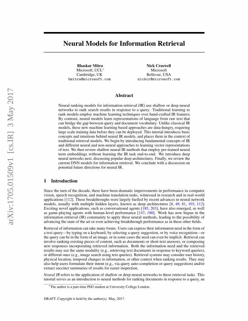
Figure 8: A vector space representation of terms puts “banana” closer to “mango” because they sharemore common attributes than “banana” and “dog”.

When the vectors are high-dimensional, sparse, and based on distributional feature they are referredto as explicit vector representations [117]. On the other hand, when the vectors are dense, small(k � |T |), and learnt from data then they are commonly referred to as embeddings. For both explicitand embedding based representations several distance metrics can be used to define similarity betweenterms, although cosine similarity is commonly used.

sim(~vi, ~vj) = cos(~vi, ~vj) =~v ᵀi ~vj

‖~vi‖‖~vj‖(23)

Most embeddings are learnt from explicit vector space representations, and hence the discussions in4.2 about different notions of similarity are also relevant to the embedding models. In Section 4.3and 4.4 we briefly discuss explicit and embedding based representations.

With respect to compositionality, it is important to understand that distributed representations ofitems are often derived from local or distributed representation of its parts. For example, a documentcan be represented by the sum of the one-hot vectors or embeddings corresponding to the terms in thedocument. The resultant vector, in both cases, corresponds to a distributed bag-of-word representation.Similarly, the character trigraph representation of terms in Figure 7d is simply an aggregation overthe one-hot representations of the constituent trigraphs.

In the context of neural models, distributed representations generally refer to learnt embeddings. Theidea of ‘local’ and ‘distributed’ representations has a specific significance in the context of neuralnetwork models. Each concept, entity, or term can be represented within a neural network by theactivation of a single neuron (local representation) or by the combined pattern of activations of severalneurons (distributed representation) [82].

4.2 Notions of similarity

Any vector representation inherently defines some notion of relatedness between terms. Is “Seattle”closer to “Sydney” or to “Seahawks”? The answer depends on the type of relationship we areinterested in. If we want terms of similar type to be closer, then “Sydney” is more similar to “Seattle”because they are both cities. However, if we are interested to find terms that co-occur in the samedocument or passage, then “Seahawks”—Seattle’s football team—should be closer. The formerrepresents a Typical, or type-based notion of similarity while the latter exhibits a more Topical senseof relatedness.

If we want to compare “Seattle” with “Sydeny” and “Seahawks based on their respective vectorrepresentations, then the underlying feature space needs to align with the notion of similarity thatwe are interested in. It is, therefore, important for the readers to build an intuition about the choiceof features and the notion of similarity they encompass. This can be demonstrated by using a toycorpus, such as the one in Table 2. Figure 9a shows that the “in documents” features naturally lend

15

Table 2: A toy corpus of short documents that we consider for the discussion on different notions ofsimilarity between terms under different distributed representations. The choice of the feature spacethat is used for generating the distributed representation determines which terms are closer in thevector space, as shown in Figure 9.

Sample documents

doc 01 Seattle map doc 09 Denver mapdoc 02 Seattle weather doc 10 Denver weatherdoc 03 Seahawks jerseys doc 11 Broncos jerseysdoc 04 Seahawks highlights doc 12 Broncos highlightsdoc 05 Seattle Seahawks Wilson doc 13 Denver Broncos Lynchdoc 06 Seattle Seahawks Sherman doc 14 Denver Broncos Sanchezdoc 07 Seattle Seahawks Browner doc 15 Denver Broncos Millerdoc 08 Seattle Seahawks Ifedi doc 16 Denver Broncos Marshall

to a Topical sense of similarity between the terms, while the “neighbouring terms with distances”features in Figure 9c gives rise to a more Typical notion of relatedness. Using “neighbouring terms”without the inter-term distances as features, however, produces a mixture of Topical and Typicalrelationships. This is because when the term distances are considered in feature definition then thedocument “Seattle Seahawks Wilson” produces the bag-of-features {Seahawks+1,Wilson+2} for“Seattle” which is non-overlapping with the bag-of-features {Seattle−1,Wilson+1} for “Seahawks”.However, when the feature definition ignores the term-distances then there is a partial overlap betweenthe bag-of-features {Seahawks,Wilson} and {Seattle,Wilson} corresponding to “Seattle” and“Seahawks”. The overlap increases significantly when we use a larger window-size for identifyingneighbouring terms pushing the notion of similarity closer to a Topical definition. This effect of thewindows size on the Topicality of the representation space was reported by Levy and Goldberg [115]in the context of learnt embeddings.

Readers should take note that the set of all inter-term relationships goes far beyond the two notionsof Typical and Topical that we discuss in this section. For example, vector representations couldcluster terms closer based on linguistic styles—e.g., terms that appear in thriller novels versus inchildren’s rhymes, or in British versus American English. However, the notions of Typical and Topicalsimilarities popularly come up in discussions in the context of many IR and NLP tasks—sometimesunder different names such as Paradigmatic and Syntagmatic relations9—and the idea itself goesback at least as far as Saussure [30, 47, 74, 172].

4.3 Explicit vector representations

Explicit vector representations can be broadly categorized based on their choice of distributionalfeatures (e.g., in documents, neighbouring terms with or without distances, etc.) and differentweighting schemes (e.g., TF-IDF, positive pointwise mutual information, etc.) applied over the rawcounts. We direct the readers to [12, 199] which are good surveys of many existing explicit vectorrepresentation schemes.

Levy et al. [117] demonstrated that explicit vector representations are amenable to the term analogytask using simple vector operations. A term analogy task involves answering questions of the form“man is to woman as king is to ____?”—the correct answer to which in this case happens to be“queen”. In NLP, term analogies are typically performed by simple vector operations of the followingform followed by a nearest-neighbour search,

9Interestingly, the notion of Paradigmatic (Typical) and Syntagmatic (Topical) relationships show up almostuniversally—not just in text. In vision, for example, the different images of “noses” bear a Typical similarityto each other, while they share a Topical relationship with images of “eyes” or “ears”. Curiously, Barthes [13]even extended this analogy to garments—where paradigmatic relationships exist between items of the same type(e.g., between hats and between boots) and the proper Syntagmatic juxtaposition of items from these differentParadigms—from hats to boots— forms a fashionable ensemble .

16

Seahawks

Denver

Broncos

Doc 02

Doc 01

Seattle

Doc 04

Doc 03

Doc 06

Doc 05

Doc 08

Doc 07

Doc 10

Doc 09

Doc 12

Doc 11

Doc 14

Doc 13

Doc 16

Doc 15

(a) “In-documents” features

Seahawks

Denver

Broncos

Denver

Seattle

Seattle

Broncos

Seahawks

weather

map

highlights

jerseys

Sherman

Wilson

Ifedi

Browner

Sanchez

Lynch

Marshall

Miller

(b) “Neighbouring terms” features

Seahawks

Denver

Broncos

Denver-1Seattle-1

Seattle

Broncos+1Seahawks+1

weather+1map+1

highlights+1jerseys+1

Wilson+2Wilson+1

Sherman+2Sherman+1

Browner+2Browner+1

Ifedi+2Ifedi+1

Lynch+2Lynch+1

Sanchez+2Sanchez+1

Miller+2Miller+1

Marshall+2Marshall+1

(c) “Neighbouring terms w/ distances” features

Figure 9: The figure shows different distributed representations for the four terms—”Seattle”,“Seahawks”, “Denver”, and “Broncos”—based on the toy corpus in Table 2. Shaded circles indicatenon-zero values in the vectors—the darker shade highlights the vector dimensions where morethan one vector has a non-zero value. When the representation is based on the documents that theterms occur in then “Seattle” is more similar to “Seahawks” than to “Denver”. The representationscheme in (a) is, therefore, more aligned with a Topical notion of similarity. In contrast, in (c)each term is represented by a vector of neighbouring terms—where the distances between the termsare taken into consideration—which puts “Seattle” closer to “Denver” demonstrating a Typical,or type-based, similarity. When the inter-term distances are ignored, as in (b), a mix of Typicaland Topical similarities is observed. Finally, it is worth noting that neighbouring-terms basedvector representations leads to similarities between terms that do not necessarily occur in the samedocument, and hence the term-term relationships are less sparse than when only in-document featuresare considered.

17

Seahawks

Denver

Broncos

Seattle

Seahawks – Seattle + Denver

Denver

Seattle

Broncos

Seahawks

weather

map

highlights

jerseys

Sherman

Wilson

Ifedi

Browner

Sanchez

Lynch

Marshall

Miller

Figure 10: A visual demonstration of term analogies via simple vector algebra. The shaded circlesdenote non-zero values. Darker shade is used to highlight the non-zero values along the vectordimensions for which the output of ~vSeahawks − ~vSeattle + ~vDenver is positive. The output vector isclosest to ~vBroncos as shown in this toy example.

~vking − ~vman + ~vwoman ≈ ~vqueen (24)

It may be surprising to some readers that the vector obtained by the simple algebraic operations~vking − ~vman + ~vwoman produces a vector close to the vector ~vqueen. We present a visual intuitionof why this works in practice in Figure 10, but we refer the readers to [7, 117] for a more rigorousmathematical explanation.

4.4 Embeddings

While explicit vector representations based on distributional features can capture interesting notionsof term-term similarity they have one big drawback—the resultant vector spaces are highly sparseand high-dimensional. The number of dimensions is generally in the same order as the number ofdocuments or the vocabulary size, which is unwieldy for most practical tasks. An alternative is tolearn lower dimensional representations of terms from the data that retains similar attributes as thehigher dimensional vectors.

An embedding is a representation of items in a new space such that the properties of, and therelationships between, the items are preserved. Goodfellow et al. [64] articulate that the goal ofan embedding is to generate a simpler representation—where simplification may mean a reductionin the number of dimensions, an increase in the sparseness of the representation, disentangling theprinciple components of the vector space, or a combination of these goals. In the context of termembeddings, the explicit feature vectors—like those we discussed in Section 4.3—constitutes theoriginal representation. An embedding trained from these features assimilate the properties of theterms and the inter-term relationships observable in the original feature space.

The most popular approaches for learning embeddings include either factorizing the term-featurematrix (e.g. LSA [48]) or using gradient descent based methods that try to predict the features giventhe term (e.g., [15, 134]). Baroni et al. [11] empirically demonstrate that these feature-predictingmodels that learn lower dimensional representations, in fact, also perform better than explicit countingbased models on different tasks—possibly due to better generalization across terms—although somecounter evidence the claim of better performances from embedding models have also been reportedin the literature [116].

The sparse feature spaces of Section 4.3 are easier to visualize and leads to more intuitiveexplanations—while their corresponding embeddings are more practically useful. Therefore, itmakes sense to think sparse, but act dense in many scenarios. In the rest of this section, we willdescribe some of the popular neural and non-neural embedding models.

Latent Semantic Analysis (LSA) LSA [48] involves performing singular value decomposition(SVD) [63] on a term-document (or term-passage) matrix X to obtain its low-rank approximation

18

[130]. SVD onX involves finding a solution toX = UΣV T , where U and V are orthogonal matricesand Σ is a diagonal matrix.10

X U Σ V ᵀ

(~dj) (~dj)↓ ↓

(~t ᵀi )→

x1,1 . . . x1,|D|

.... . .

...

x|T |,1 . . . x|T |,|D|

= (~t ᵀ

i )→

~u1

. . .~ul ·

σ1 . . . 0...

. . ....

0 . . . σl

·[ ~v1 ]

...[ ~vl ]

(25)

where, σ1, . . . , σl, ~u1, . . . , ~ul, and ~v1, . . . ,~vl are the singular values, the left singular vectors, and theright singular vectors, respectively. The k largest singular values, and corresponding singular vectorsfrom U and V , is the rank k approximation of X (Xk = UkΣkV

Tk ). The embedding for the ith term

is given by Σk~ti.

While LSA operate on a term-document matrix, matrix factorization based approaches can also beapplied to term-term matrices [25, 111, 168].

Neural term embedding models are typically trained by setting up a prediction task. Instead offactorizing the term-feature matrix—as in LSA—neural models are trained to predict the termfrom its features. Both the term and the features have one-hot representations in the input andthe output layers, respectively, and the model learns dense low-dimensional representations in theprocess of minimizing the prediction error. These approaches are based on the information bottleneckmethod [197]—discussed in more details in Section 6.2—with the low-dimensional representationsacting as the bottleneck. The training data may contain many instances of the same term-featurepair proportional to their frequency in the corpus (e.g., word2vec [134]), or their counts can bepre-aggregated (e.g., GloVe [160]).

Word2vec For word2vec [61, 134, 136, 137, 169], the features for a term are made up of itsneighbours within a fixed size window over the text from the training corpus. The skip-gramarchitecture (see Figure 11a) is a simple one hidden layer neural network. Both the input and theoutput of the model is in the form of one-hot vectors and the loss function is as follows,

Lskip−gram = − 1

|S|

|S|∑i=1

∑−c≤j≤+c,j 6=0

log(p(ti+j |ti)) (26)

where, p(ti+j |ti) =exp ((Wout~vti+j

)ᵀ(Win~vti))∑|T |k=1 exp ((Wout~vtk)ᵀ(Win~vti))

(27)

S is the set of all windows over the training text and c is the number of neighbours we need to predicton either side of the term ti. The denominator for the softmax function for computing p(ti+j |ti) sumsover all the words in the vocabulary. This is prohibitively costly and in practice either hierarchical-softmax [149] or negative sampling is employed. Also, note that the model has two different weightmatrices Win and Wout that are learnable parameters of the models. Win gives us the IN embeddingscorresponding to all the input terms and Wout corresponding to the OUT embeddings for the outputterms. Generally, only Win is used and Wout is discarded after training, but we will discuss an IRapplication that makes use of both the IN and the OUT embeddings later in Section 5.1.

The continuous bag-of-words (CBOW) architecture (see Figure 11b) is similar to the skip-grammodel, except that the task is to predict the middle term given the sum of the one-hot vectorsof the neighbouring terms in the window. Given a middle term ti and the set of its neigbours

10The matrix visualization is adapted from https://en.wikipedia.org/wiki/Latent_semantic_analysis.

19

Win Wout

ti ti+j

(a) Skip-gram

WinWout

t i+2

t i+1

t i-2

t i-1

ti*

ti

(b) Continuous bag-of-words (CBOW)

Figure 11: The (a) skip-gram and the (b) continuous bag-of-words (CBOW) architectures of word2vec.The architecture is a neural network with a single hidden layer whose size is much smaller than thatof the input and the output layers. Both models use one-hot representations of terms in the inputand the output. The learnable parameters of the model comprise of the two weight matrices Win

and Wout that corresponds to the embeddings the model learns for the input and the output terms,respectively. The skip-gram model trains by minimizing the error in predicting a term given one ofits neighbours. The CBOW model, in contrast, predicts a term from a bag of its neighbouring terms.

20

{ti−c, . . . , ti−1, ti+1, . . . , ti+c}, the CBOW model creates a single training sample with the sum ofthe one-hot vectors of all the neighbouring terms as input and the one-hot vector ~vti , correspondingto the middle term, as the expected output.

LCBOW = − 1

|S|

|S|∑i=1

log(p(ti|∑

−c≤j≤+c,j 6=0

ti+j)) (28)

Contrast this with the skip-gram model that creates 2× c samples by individually pairing each of theneighbouring terms with the middle term. During training, given the same number of windows oftext, the skip-gram model, therefore, trains orders of magnitude slower than the CBOW model [134]because it creates 2× c the number of training samples.

Word2vec gained particular popularity for its ability to perform word analogies using simple vectoralgebra, similar to what we have already discussed in Section 4.3. For domains where the inter-pretability of the embeddings may be important, Sun et al. [191] introduced an additional constraintin the loss function to encourage more sparseness in the learnt representation.

Lsparse−CBOW = Lsparse−CBOW − λ∑t∈T‖~vt‖1 (29)

GloVe The skip-gram model trains on individual term-neighbour pairs. If we aggregate all thetraining samples into a matrix X , such that xij is the frequency of the pair 〈ti, tj〉 in the training data,then the loss function changes to,

Lskip−gram = −|T |∑i=1

|T |∑j=1

xij log(p(ti|tj)) (30)

= −|T |∑i=1

xi

|T |∑j=1

xijxilog(p(ti|tj)) (31)

= −|T |∑i=1

xi

|T |∑j=1

p(ti|tj)log(p(ti|tj)) (32)

=

|T |∑i=1

xiH(p(ti|tj)log(p(ti|tj))) (33)

H(. . . ) is the cross-entropy error between the actual co-occurrence probability p(ti|tj) and the onepredicted by the model p(ti|tj). This is similar to the loss function for GloVe [160] if we replacethe cross-entropy error with a squared-error and apply a saturation function f(. . . ) over the actualco-occurrence frequencies.

LGloV e = −|T |∑i=1

|T |∑j=1

f(xij)(log(xij − ~v ᵀwi~vwj ))2 (34)

GloVe is trained using AdaGrad [53]. Similar to word2vec, GloVe also generates two different (INand OUT) embeddings, but unlike word2vec it generally uses the sum of the IN and the OUT vectorsas the embedding for each term in the vocabulary.

Paragraph2vec Following the popularity of word2vec [134, 136], similar neural architectures[4, 5, 68, 69, 110, 189] have been proposed that trains on term-document co-occurrences. Thetraining typically involves predicting a term given the ID of a document or a passage that contains theterm. In some variants, as shown in Figure 12, neighbouring terms are also provided as input.

21

Wd,in Wt,out

dj ti

ti+2ti+1ti-2 ti-1

Wt,in

Figure 12: The paragraph2vec architecture as proposed by Le and Mikolov [110] trains by predictinga term given a document (or passage) ID containing the term. By trying to minimize the predictionerror, the model learns an embedding for the term as well as for the document. In some variants ofthe architecture, optionally the neighbouring terms are also provided as input—as shown in the dottedbox.

The key motivation for training on term-document pairs is to learn an embedding that is more alignedwith a Topical notion of term-term similarity—which is often more appropriate for IR tasks. Theterm-document relationship, however, tends to be more sparse [219]—including neighbouring termfeatures may compensate for some of that sparsity.

In the context of IR tasks, Ai et al. [4, 5] proposed a number of IR-motivated changes to the originalParagraph2vec [110] model training—including, document frequency based negative sampling anddocument length based regularization.

5 Term embeddings for IR

Traditional IR models use local representations of terms for query-document matching. The moststraight-forward use case for term embeddings in IR is to enable inexact matching in the embeddingspace. In Section 2.2, we argued the importance of inspecting non-query terms in the document forgarnering evidence of relevance. For example, even from a shallow manual inspection, it is easy toconclude that the passage in Figure 13a is about Albuquerque because it contains “metropolitan”,“population”, and “area” among other informative terms. On the other hand, the passage in Figure 13bcontains “simulator”, “interpreter”, and “Altair” which seems to suggest that the passage is insteadmore likely related to computers and technology. In traditional term counting based IR approachesthese signals are often ignored.

22

Albuquerque is the most populous city in the U.S.state of New Mexico. The high-altitude city servesas the county seat of Bernalillo County, and it issituated in the central part of the state, straddling theRio Grande. The city population is 557,169 as ofthe July 1, 2014 population estimate from the UnitedStates Census Bureau, and ranks as the 32nd-largestcity in the U.S. The Albuquerque metropolitan sta-tistical area (or MSA) has a population of 907,301according to the United States Census Bureau’s mostrecently available estimate for 2015.

(a) About Albuquerque

Allen suggested that they could program a BASICinterpreter for the device; after a call from Gatesclaiming to have a working interpreter, MITS re-quested a demonstration. Since they didn’t actuallyhave one, Allen worked on a simulator for the Al-tair while Gates developed the interpreter. Althoughthey developed the interpreter on a simulator and notthe actual device, the interpreter worked flawlesslywhen they demonstrated the interpreter to MITS inAlbuquerque, New Mexico in March 1975; MITSagreed to distribute it, marketing it as Altair BASIC.

(b) Not about Albuquerque

Figure 13: Two passages both containing exactly a single occurrence of the query term “Albuquerque”.However, the passage in (a) contains other terms such as “population” and “area” that are relevant toa description of the city. In contrast, the terms in passage (b) suggest that it is unlikely to be about thecity, and only mentions the city potentially in a different context.

Most existing shallow neural methods for IR focus on inexact matching using term embeddings.These approaches can be broadly categorized as those that compare the query with the documentdirectly in the embedding space; and those that use embeddings to generate suitable query expansioncandidates from a global vocabulary and then perform retrieval based on the expanded query. Wediscuss both these classes of approaches in the remainder of this section.

5.1 Query-document matching

A popular strategy for using term embeddings in IR involves deriving a dense vector representation forthe query and the document from the embeddings of the individual terms in the corresponding texts.The term embeddings can be aggregated in different ways, although using the average word (or term)embeddings (AWE) is quite popular [96, 101, 110, 143, 151, 190, 207]. Non-linear combinations ofterm vectors—such as using Fisher Kernel Framework [35]—have also been explored, as well asother families of aggregate functions of which AWE has been shown to be a special case [228].

The query and the document embeddings themselves can be compared using a variety of similaritymetrics, such as cosine similarity or dot-product. For example,

sim(q, d) = cos(~vq, ~vd) =~v ᵀq ~vd

‖~vq‖‖~vd‖(35)

where, ~vq =1

|q|∑tq∈q

~vtq‖~vtq‖

(36)

~vd =1

|d|∑td∈d

~vtd‖~vtd‖

(37)

An important consideration here is the choice of the term embeddings that is appropriate for theretrieval scenario. While, LSA [48], word2vec [136], and GloVe [160] are popularly used—it isimportant to understand how the notion of inter-term similarity modelled by a specific vector spacemay influence its performance on a retrieval task. In the example in Figure 13, we want to rankdocuments that contains related terms, such as “population” or “area” higher—these terms areTopically similar to the query term “Albuquerque”. Intuitively, a document about “Tucson”—which isTypically similar to “Albuquerque”—is unlikely to satisfy the user intent. The discussion in Section4.2 on how input features influence the notion of similarity in the learnt vector space is relevant here.

Models, such as LSA [48] and Paragraph2vec [110], that consider term-document pairs generallycapture Topical similarities in the learnt vector space. On the other hand, word2vec [136] and GloVe[160] embeddings may incorporate a mixture of Topical and Typical notions of relatedness. These

23

neural models behave more Typical when trained with short window sizes or on short text, such as onkeyword queries [115] (refer to Section 4.2 for more details).

In Section 4.4, we made a note that the word2vec model learns two different embeddings—INand OUT—corresponding to the input and the output terms. Mitra et al. [143] point out that whenusing word2vec embeddings for IR it is more appropriate to represent the query terms using theIN embeddings and the document terms using the OUT embeddings of the trained model. In thisDual Embedding Space Model (DESM)11 [143, 151] the word2vec embeddings are trained on searchqueries, which empirically performs better than training on document body text. Training on shortqueries, however, makes the inter-term similarity more pronouncedly Typical (where, “Yale” is closerto “Harvard” and “NYU”) when both terms are represented using their IN vectors—better retrievalperformance is achieved instead by using the IN-OUT similarity (where, “Yale” is closer to “faculty”and “alumni”) that mirrors more the Topical notions of relatedness.

DESMin−out(q, d) =1

|q|∑tq∈q

~v ᵀtq,in

~vd,out

‖~vtq,in‖‖~vd,out‖(38)

~vd,out =1

|d|∑td∈d

~vtd,out‖~vtd,out‖

(39)

An alternative to representing queries and documents as an aggregate of their term embeddings isto incorporate the term representations into existing IR models, such as the ones we discussed inSection 2.5. Zuccon et al. [236] proposed the Neural Translation Language Model (NTLM) that usesthe similarity between term embeddings as a measure for term-term translation probability p(tq|td)in Equation 15.

p(tq|td) =cos(~vtq , ~vtd)∑t∈T cos(~vt, ~vtd)

(40)

On similar lines, Ganguly et al. [58] proposed the Generalized Language Model (GLM) whichextends the Language Model based approach in Equation 13 to,

p(d|q) =∏tq∈q

(λtf(tq, d)

|d|+ α

∑td∈d (sim(~vtq , ~vtd) · tf(td, d))∑

td1∈d∑td2∈d sim(~vtd1

, ~vtd2) · |d|2

+ β

∑t∈Nt

(sim(~vtq , ~vt) ·∑d∈D tf(t, d))∑

td1∈Nt

∑td2∈Nt

sim(~vtd1, ~vtd2

) ·∑d∈D |d| · |Nt|

+ (1− α− β − λ)

∑d∈D tf(tq, d)∑

d∈D |d|

)(41)

where, Nt is the set of nearest-neighbours of term t. Ai et al. [4] incorporate paragraph vectors [110]into the query-likelihood model [161].

Another approach, based on the Earth Mover’s Distance (EMD) [171], involves estimating similaritybetween pairs of documents by computing the minimum distance in the embedding space that eachterm in the first document needs to travel to reach the terms in the second document. This measure,commonly referred to as the Word Mover’s Distance (WMD), was originally proposed by Wan et al.[210, 211], but used WordNet and topic categories instead of distributed representations for definingdistance between terms. Term embeddings were later incorporated into the model by Kusner et al.[87, 104]. Finally, Guo et al. [72] incorporated similar notion of distance into the Non-linear WordTransportation (NWT) model that estimates relevance between a a query and a document. The NWTmodel involves solving the following constrained optimization problem,

11The dual term embeddings trained on Bing queries is available for download at https://www.microsoft.com/en-us/download/details.aspx?id=52597

24

max∑tq∈q

log

( ∑td∈u(d)

f(tq, td) ·max(cos(~vtq , ~vtd), 0

)idf(tq)+b)

(42)

subject to f(tq, td) ≥ 0, ∀tq ∈ q, td ∈ d (43)

and∑tq∈q

f(tq, td) =tf(td) + µ

∑d∈D tf(tq,d)∑

d∈D |d|

|d|+ µ, ∀td ∈ d (44)

where, idf(t) =|D| − df(t) + 0.5

df(t) + 0.5(45)

u(d) is the set of all unique terms in document d, and b is a constant.

Another term-alignment based distance metric was proposed by Kenter and de Rijke [98] for comput-ing short-text similarity. The design of the saliency-weighted semantic network (SWSN) is motivatedby the BM25 [166] formulation.

swsn(sl, ss) =∑tl∈sl

idf(tl) ·sem(tl, ss) · (k1 + 1)

sem(tl, ss) + k1 ·(

1− b+ b · |ss|avgsl

) (46)

where, sem(t, s) = maxt∈s

cos(~vt, ~vt) (47)

Here ss is the shorter of the two sentences to be compared, and sl the longer sentence.

Telescoping evaluation Figure 14 highlights the distinct strengths and weaknesses of matchingusing local and distributed representations of terms for retrieval. For the query “Cambridge”, alocal representation (or exact matching) based model can easily distinguish between the passage onCambridge (Figure 14a) and the one on Oxford (Figure 14b). However, the model is easily duped byan non-relevant passage that has been artificially injected with the term “Cambridge” (Figure 14d).The distributed representation based matching, on the other hand, can spot that the other terms in thepassage provide clear indication that the passage is not about a city, but fails to realize that the thepassage about Oxford (Figure 14b) is inappropriate for the same query.

Embedding based models often perform poorly when the retrieval is performed over the full documentcollection [143]. However, as seen in the example of Figure 14, the errors made by embeddingbased models and exact matching models are typically different—and the combination of the twoperforms better than exact matching models alone [4, 58, 143]. Another popular technique is touse the embedding based model to re-rank only a subset of the documents retrieved by a different—generally an exact matching based—IR model. The chaining of different IR models where eachsuccessive model re-ranks a smaller number of candidate documents is called Telescoping [131].Telescoping evaluations are popular in the neural IR literature [71, 88, 141, 143, 177] and the resultsare representative of performances of these models on re-ranking tasks. However, as Mitra et al. [143]demonstrate, good performances on re-ranking tasks may not be indicative how the model wouldperform if the retrieval involves larger document collections.

5.2 Query expansion

Instead of comparing the query and the document directly in the embedding space, an alternativeapproach is to use term embeddings to find good expansion candidates from a global vocabulary,and then retrieving documents using the expanded query. Different functions [51, 170, 227] havebeen proposed for estimating the relevance of candidate terms to the query—all of them involvescomparing the candidate term individually to every query term using their vector representations, andthen aggregating the scores. For example, [51, 170] estimate the relevance of candidate term tc as,

score(tc, q) =1

|q|∑tq∈q

cos(~vtc , ~vtq ) (48)

25

the city of cambridge is a university city and the county town of cambridgeshire ,

england . it lies in east anglia , on the river cam , about 50 miles ( 80 km ) north of london . according to the united kingdom

census 2011 , its population was 123867 ( including 24488 students ) . this makes cambridge the second largest

city in cambridgeshire after peterborough , and the 54th largest in the united kingdom . there is archaeological

evidence of settlement in the area during the bronze age and roman times ; under viking rule cambridgebecame an important trading centre . the first town charters were granted in the 12th century , although city status was not

conferred until 1951 .

(a) Passage about the city of Cambridge

oxford is a city in the south east region of england and the county town of oxfordshire . with a population of

159994 it is the 52nd largest city in the united kingdom , and one of the fastest growing and most ethnically diverse . oxford has

a broad economic base . its industries include motor manufacturing , education , publishing and a large number of

information technology and sciencebased businesses , some being academic offshoots . the city is known worldwide as the home

of the university of oxford , the oldest university in the englishspeaking world . buildings in oxford demonstrate examples of every

english architectural period since the arrival of the saxons , including the mid18thcentury radcliffe camera . oxford is known as the cityof dreaming spires , a term coined by poet matthew arnold .

(b) Passage about the city of Oxford

the giraffe ( giraffa camelopardalis ) is an african eventoed ungulate mammal , the tallest living terrestrial animal and the largest ruminant . its

species name refers to its camellike shape and its leopardlike colouring . its chief distinguishing characteristics are its extremely long neck and legs , its hornlike ossicones , and its

distinctive coat patterns . it is classified under the family giraffidae , along with its closest extant relative , the okapi . the nine subspecies are

distinguished by their coat patterns . the scattered range of giraffes extends from chad in the north to south africa in the south , and

from niger in the west to somalia in the east . giraffes usually inhabit savannas , grasslands , and open woodlands .

(c) Passage about giraffes

the cambridge ( giraffa camelopardalis ) is an african eventoed ungulate mammal , the tallest living terrestrial animaland the largest ruminant . its species name refers to its camellike shape and its leopardlike colouring . its chief distinguishing characteristics are its extremely long

neck and legs , its hornlike ossicones , and its distinctive coat patterns . it is classified under the family giraffidae , along with its closest extant relative , the

okapi . the nine subspecies are distinguished by their coat patterns . the scattered range of giraffes extends from chad in the north to

south africa in the south , and from niger in the west to somalia in the east . giraffes usually inhabit savannas , grasslands , and open

woodlands .

(d) Passage about giraffes, but ’giraffe’ is replaced by ’Cambridge’

Figure 14: A visualization of IN-OUT similarities between terms in different passages with thequery term “Cambridge”. The visualization—adapted from https://github.com/bmitra-msft/Demos/blob/master/notebooks/DESM.ipynb—reveal that, besides the term “Cambridge”, manyother terms in the passages about both Cambridge and Oxford have high similarity to the queryterm. The passage (d) is adapted from the passage (c) on giraffes by replacing all the occurrencesof the term “giraffe” with “cambridge”. However, none of the other terms in (d) are found to berelevant to the query term. An embedding based approach may be able to determine that passage (d)is non-relevant to the query “Cambridge”, but fail to realize that passage (b) is also non-relevant. Aterm counting-based model, on the other hand, can easily identify that passage (b) is non-relevant,but may rank passage (d) incorrectly high.

26

(a) Global embedding (b) Local embedding

Figure 15: A two-dimensional visualization of term embeddings when the vector space is trained ona (a) global corpus and a (b) query-specific corpus, respectively. The grey circles represent individualterms in the vocabulary. The white circle represents the query “‘ocean remote sensing” by averagingthe embeddings of the individual terms in the query, and the light grey circles correspond to goodexpansion terms for this query. When the representations are query-specific then the meaning of theterms are better disambiguated, and more likely to result in the selection of good expansion terms.

Term embedding based query expansion on its own performs worse than pseudo-relevance feed-back [170]. But like the models in the previous section, shows better performances when used incombination with PRF [227].

Diaz et al. [51] explored the idea of query-specific term embeddings and found that they are muchmore effective in identifying good expansion terms than a global representation (see Figure 15). Thelocal model proposed by Diaz et al. [51] incorporate relevance feedback in the process of learning theterm embeddings—a set of documents is retrieved for the query and a query-specific term embeddingmodel is trained. This local embedding model is then employed for identifying expansion candidatesfor the query for a second round of document retrieval.

Term embeddings have also been explored for re-weighting query terms [233] and finding relevantquery re-writes [69], as well as in the context of other IR tasks such as cross-lingual retrieval [207]and entity retrieval [200]. In the next section, we move on to neural network models with deeperarchitectures and their applications to retrieval.

6 Deep neural networks

Deep neural network models consist of chains of tensor operations. The tensor operation can rangefrom parameterized linear transformations (e.g., multiplication with a weight matrix, addition of abias vector) to elementwise application of non-linear functions, such as tanh or rectified linear units(ReLU) [73, 89, 150]. Figure 16 shows a simple feed-forward neural network with fully-connectedlayers. For an input vector ~x, the model produces the output ~y as follows,

~y = tanh(W2 · tanh(W1 · ~x+~b1) +~b2) (49)

The model training involves tuning the parameters W1,~b1, W2, and~b2 to minimize the loss betweenthe expected output and the actual output of the final layer. The parameters are usually traineddiscriminatively using backpropagation [14, 77, 175]. During forward-pass each layer generates anoutput conditioned on its input, and during backward pass each layer computes the error gradientwith respect to its parameters and its inputs.

The design of a DNN typically involves many choices of architectures and hyper-parameters. Neuralnetworks with as few a single hidden layer—but with sufficient number of hidden nodes—can

27

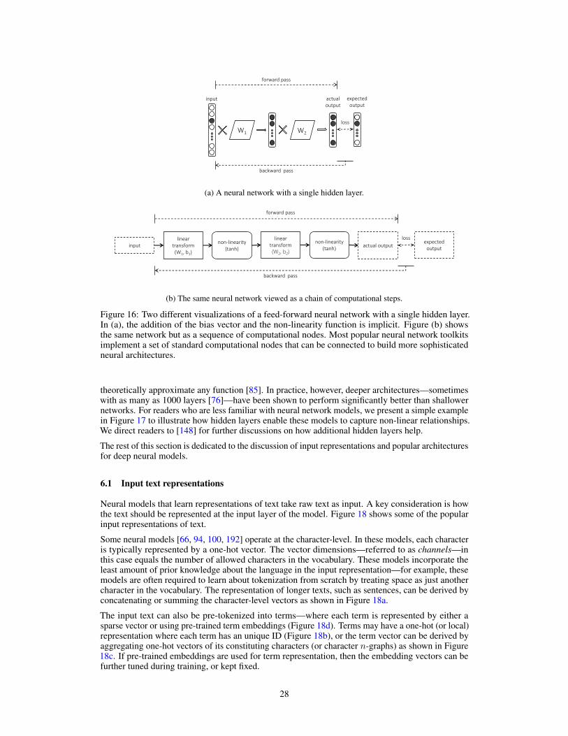
forward pass

backward pass

W1 W2

input actual

output

loss

expected

output

(a) A neural network with a single hidden layer.

non-linearity

(tanh)input

linear

transform

(W1, b1)

non-linearity

(tanh)

linear

transform

(W2, b2)

actual output

forward pass

backward pass

expected

output

loss

(b) The same neural network viewed as a chain of computational steps.

Figure 16: Two different visualizations of a feed-forward neural network with a single hidden layer.In (a), the addition of the bias vector and the non-linearity function is implicit. Figure (b) showsthe same network but as a sequence of computational nodes. Most popular neural network toolkitsimplement a set of standard computational nodes that can be connected to build more sophisticatedneural architectures.

theoretically approximate any function [85]. In practice, however, deeper architectures—sometimeswith as many as 1000 layers [76]—have been shown to perform significantly better than shallowernetworks. For readers who are less familiar with neural network models, we present a simple examplein Figure 17 to illustrate how hidden layers enable these models to capture non-linear relationships.We direct readers to [148] for further discussions on how additional hidden layers help.

The rest of this section is dedicated to the discussion of input representations and popular architecturesfor deep neural models.

6.1 Input text representations

Neural models that learn representations of text take raw text as input. A key consideration is howthe text should be represented at the input layer of the model. Figure 18 shows some of the popularinput representations of text.

Some neural models [66, 94, 100, 192] operate at the character-level. In these models, each characteris typically represented by a one-hot vector. The vector dimensions—referred to as channels—inthis case equals the number of allowed characters in the vocabulary. These models incorporate theleast amount of prior knowledge about the language in the input representation—for example, thesemodels are often required to learn about tokenization from scratch by treating space as just anothercharacter in the vocabulary. The representation of longer texts, such as sentences, can be derived byconcatenating or summing the character-level vectors as shown in Figure 18a.

The input text can also be pre-tokenized into terms—where each term is represented by either asparse vector or using pre-trained term embeddings (Figure 18d). Terms may have a one-hot (or local)representation where each term has an unique ID (Figure 18b), or the term vector can be derived byaggregating one-hot vectors of its constituting characters (or character n-graphs) as shown in Figure18c. If pre-trained embeddings are used for term representation, then the embedding vectors can befurther tuned during training, or kept fixed.

28

Input features Hidden layersLabel

surface kerberos book library H1 H2

1 0 1 0 1 0 ✓1 1 0 0 0 0 ✗0 1 0 1 0 1 ✓0 0 1 1 0 0 ✗

library booksurface kerberos

+0.5 +0.5

-1

-1 -1

-1

+1 +1

+0.5 +0.5

H1 H2

Figure 17: Consider a toy binary classification task on a corpus of four short texts—“surface book”,“kerberos library”, “library book”, and “kerberos surface”—where the model needs to predict if thetext is related to computers. The first two texts—“Surface Book” and “kerberos library”—are positiveunder this classification, and the latter two negative. The input feature space consists of four binaryfeatures that indicate whether each of the four terms from the vocabulary is present in the text. Thetable shows that the specified classes are not linearly separable with respect to the input feature space.However, if we add couple of hidden nodes, as shown in the diagram, then the classes can be linearlyseparated with respect to the output of the hidden layer.

Similar to character-level models, the term vectors are further aggregated (by concatenation or sum)to obtain the representation of longer chunks of text, such as sentences. While one-hot representationsof terms (Figure 18b) are common in many NLP tasks, pre-trained embeddings (e.g., [86, 158]) andcharacter n-graph based representations (e.g., [88, 141]) are more popularly employed in IR.

6.2 Popular architectures

In this section, we describe few neural operations and architectures popular in IR. For broaderoverview of different neural architectures and design patterns please refer to [64, 112, 175].

Shift-invariant neural operations Convolutional [89, 103, 113, 114] and recurrent [67, 83, 135,173] architectures are commonplace in most deep learning applications. These neural operations arepart of a broader family of shift-invariant architectures. The key intuition behind these architecturesstem from the natural regularities observable in most inputs. In vision, for example, the task ofdetecting a face should be invariant to whether the image is shifted, rotated, or scaled. Similarly, themeaning of an English sentence should, in most cases, stay consistent independent of which partof the document it appears in. Therefore, intuitively a neural model for object recognition or textunderstanding should not learn an independent logic for the same action applied to different parts ofthe input space.

All shift-invariant neural operations fundamentally employ a window-based approach. A fixed sizewindow is moved over the input space with fixed stride in each step. A (typically parameterized)function—referred to as a kernel, or a filter, or a cell—is applied over each instance of the window.The parameters of the cell are shared across all the instances of the input window. The sharedparameters not only implies less number of total parameters in the model„ but also more supervisionper parameter per training sample due to the repeated application.

Figure 19a shows an example of a cell being applied on a sequence of terms—with a window sizeof three terms—in each step. A popular cell implementation involves multiplying with a weightmatrix—in which case the architecture in Figure 19a is referred as convolutional. An example of acell without any parameters is pooling—which consists of aggregating (e.g., by computing the maxor the average) over all the terms in the window12. Note, that the length of the input sequence can bevariable in both cases and the length of the output of a convolutional (or pooling) layer is a function ofthe input length. Figure 19b shows an example of global pooling—where the window spans over the

12If the input has multiple channels per term then the aggregation is performed per channel.

29

d o g s h a v e o w n e r s c a t s h a v e s t a f f

one-h

ot

vect

ors

concatenate

chan

nels

[chars x channels]

(a) Character-level input

d o g s h a v e o w n e r s c a t s h a v e s t a f f

one-h

ot

vect

ors

concatenate

sum sum sum sum sum sum

chan

nels

[words x channels]

(b) Term-level input w/ bag-of-characters per term

# d o g s # # h a v e # # o w n e r s # # c a t s # # h a v e # # s t a f f #

one-h

ot

vect

ors

concatenate or sum

sum sum sum sum sum sum

chan

nels

[words x channels] or [1 x channels]

(c) Term-level input w/ bag-of-trigraphs per term

d o g s h a v e o w n e r s c a t s h a v e s t a f f

pre

-tra

ined

em

bed

din

gs

concatenate or sum

chan

nels

[words x channels] or [1 x channels]

(d) Term-level input w/ pre-trained term embeddings

Figure 18: Examples of different representation strategies for text input to deep neural networkmodels. The smallest granularity of representation can be a character or a term. The vector can be asparse local representation, or a pre-trained embedding.

30

output

(a) Convolution or pooling

convolution

pooling

output

(b) Convolution w/ global pooling

output

(c) Recurrent

output

(d) Recursive or tree

Figure 19: Popular shift-invariant neural architectures including convolutional neural networks(CNN), recurrent neural networks (RNN), pooling layers, and tree-structured neural networks.

whole input—being applied on top of a convolutional layer. The global pooling strategy is commonfor generating a fixed size output from a variable length input.13

In convolution or pooling, each window is applied independently. In contrast, in the recurrentarchitecture of Figure 19c the cell not only considers the input window but also the output of theprevious instance of the cell as its input. Many different cell architectures have been explored forrecurrent neural networks (RNN)—although Elman network [54], Long Short-Term Memory (LSTM)[83], and Gated Recurrent Unit (GRU) [32, 34] are popular. RNNs are popularly applied to sequences,but can also be useful for two (and higher) dimensional inputs [209].

One consideration when using convolutional or recurrent layers is how the window outputs areaggregated. Convolutional layers are typically followed by pooling or fully-connected layers thatperform a global aggregation over all the window instances. While a fully-connected layer is awareof each window position, a global pooling layer is typically agnostic to it. However, unlike a fully-connected layer, a global max-pooling operation can be applied to a variable size input. Where aglobal aggregation strategy may be less appropriate (e.g., long sequences), recurrent networks withmemory [18, 188, 213] and/or attention [33, 78, 126, 146, 217] may be useful.

Finally, Figure 19c shows tree-structured (or recursive) neural networks [20, 62, 182, 183, 195]where the same cell is applied at multple levels in a tree-like hierarchical fashion.

13It is obvious, but may be still worth pointing out, that a global convolutional layer is exactly the same as afully-connected layer.

31

input output

embedding

encode decode

(a) Auto-encoder

input1 input2

embedding1

model1

similarityfunction

embedding2

model2

(b) Siamese network

Figure 20: Both (a) the auto-encoder and (b) the Siamese network architectures are designed to learncompressed representations of inputs. In an auto-encoder the embeddings are learnt by minimizingthe self-reconstruction error, whereas a Siamese network focuses on retaining the information that isnecessary for determining the similarity between a pair of items (say, a query and a document).

Auto-encoders The auto-encoder architecture [14, 16, 164] is based on the information bottleneckmethod [197]. The goal is to learn a compressed representation ~x ∈ Rk of items from their higher-dimensional vector representations ~v ∈ RK , such that k � K. The model has an hour-glass shape asshown in Figure 20a and is trained by feeding in the high-dimensional vector inputs and trying tore-construct the same representation at the output layer. The lower-dimensional middle layer forcesthe encoder part of the model to extract the minimal sufficient statistics of ~v into ~x, such that thedecoder part of the network can reconstruct the original input back from ~x. The model is trained byminimizing the reconstruction error between the input ~v and the actual output of the decoder ~v′. Thesquared-loss is popularly employed.

Lauto−encoder(~v, ~v′) = ‖~v − ~v′‖2 (50)

Siamese networks Siamese networks were originally proposed for comparing fingerprints [10]and signatures [21]. Yih et al. [222] later adapted the same architecture for comparing short texts.

The siamese network, as seen in Figure 20b, resembles the auto-encoder architecture (if you squinthard enough!)—but unlike the latter is trained on pairs of inputs 〈input1, input2〉. The architectureconsists of two models (model1 and model2) that project input1 and input2, respectively, to ~v1

and ~v2 in a common embedding space. A pre-defined metric (e.g., cosine similarity) is used to thencompute the similarity between ~v1 and ~v2. The model parameters are optimized such that ~v1 and ~v2

are closer when the two inputs are expected to be similar, and further away otherwise.

One possible loss function is the logistic loss. If each training sample consist of a triple 〈~vq, ~vd1, ~vd2〉,such that sim(~vq, ~vd1) should be greater than sim(~vq, ~vd2), then we minimize,

Lsiamese(~vq, ~vd1, ~vd2) = log(

1 + eγ(sim( ~vq, ~vd2)−sim( ~vq, ~vd1)))

(51)

where, γ is a constant that is often set to 10. Typically both the models—model1 and model2—shareidentical architectures, but can also choose to share the same parameters.

It is important to note that, unlike the auto-encoder, the minimal sufficient statistics retained by aSiamese network is dictated by which information it deems important for determining the similaritybetween the paired items.

32

6.3 Neural toolkits

In recent years, the advent of numerous flexible toolkits [1, 6, 31, 38, 91, 152, 198, 225] hashad a catalytic influence on the area of neural networks. Most of the toolkits define a set ofcommon neural operations that—like Lego14 blocks—can be composed to build complex networkarchitectures.15 Each instance of these neural operations or computation nodes can have associatedlearnable parameters that are updated during training, and these parameters can be shared betweendifferent parts of the network if necessary. Every computation node under this framework mustimplement the appropriate logic for,

• computing the output of the node given the input (forward-pass)

• computing the gradient of the loss with respect to the inputs, given the gradient of the losswith respect to the output (backward-pass)

• computing the gradient of the loss with respect to its parameters, given the gradient of theloss with respect to the output (backward-pass)

A deep neural network, such as the one in Figure 16 or ones with much more complex architectures(e.g., [76, 107, 193]), can then be specified by chaining instances of these available computationnodes, and trained end-to-end on large datasets using backpropagation over GPUs or CPUs. In IR,various application interfaces [142, 201] bind these neural toolkits with existing retrieval/indexingframeworks, such as Indri [186].

Refer to [179] for a comparison of different neural toolkits based on their speed of training usingstandard performance benchmarks.

7 Deep neural models for IR

Traditionally, deep neural network models have much larger number of learnable parameters thantheir shallower counterparts. A DNN with a large set of parameters can easily overfit to smallertraining datasets [231]. Therefore, during model design it is typical to strike a balance between thenumber of model parameters and the size of the data available for training. Data for ad-hoc retrievalmainly consists of,

• Corpus of search queries

• Corpus of candidate documents

• Ground truth—in the form of either explicit human relevance judgments or implicit labels(e.g., from clicks)—for query-document pairs

While both large scale corpora of search queries [46, 159] and documents [9, 29, 45] are publiclyavailable for IR research, the amount of relevance judgments that can be associated with them areoften limited outside of large industrial research labs—mostly due to user privacy concerns. Wenote that we are interested in datasets where the raw text of the query and the document is available.Therefore, this excludes large scale public labelled datasets for learning-to-rank (e.g., [122]) thatdon’t contain the textual contents.

The proportion of labelled and unlabelled data that is available influences the level of supervisionthat can be employed for training these deep models. Most of the models we covered in Section 5operate under the data regime where large corpus of documents or queries is available, but limited(or no) labelled data. Under such settings where no direct supervision or relevance judgments isprovided, typically an unsupervised approach is employed (e.g., [174]). The unlabelled document(or query) corpus is used to learn good text representations, and then these learnt representations areincorporated into an existing retrieval model or a query-document similarity metric. If small amountsof labelled data are available, then that can be leveraged to train a retrieval model with few parametersthat in turn uses text representations that is pre-trained on larger unlabelled corpus. Examples ofsuch semi-supervised training includes models such as [71, 157, 158]. In contrast, fully-supervised

14https://en.wikipedia.org/wiki/Lego15http://www.inference.vc/content/images/2016/01/9k-.jpg

33

Table 3: Comparing the nearest neighbours for "seattle" and "taylor swift" in the CDSSM embeddingspaces when the model is trained on query-document pairs vs. query prefix-suffix pairs. The formerresembles a Topical notion of similarity between terms, while the latter is more Typical in thedefinition of inter-term similarities.

seattle taylor swiftQuery-Document Prefix-Suffix Query-Document Prefix-Suffix

weather seattle chicago taylor swift.com lady gagaseattle weather san antonio taylor swift lyrics meghan trainor

seattle washington denver how old is taylor swift megan trainorikea seattle salt lake city taylor swift twitter nicki minaj

west seattle blog seattle wa taylor swift new song anna kendrick

models such as [37, 88, 141, 176], optimize directly for the target task by training on large number oflabelled query-document pairs.

It is also useful to distinguish between deep neural models that focus on ranking long documents,from those that rank short texts (e.g., for the question-answering task, or for document rankingwhere the document representation is based on the title or on clicked queries). The challenges inshort text ranking are somewhat distinct from those involved in the ad-hoc retrieval task [36]. Whencomputing similarity between pairs of short-texts, vocabulary mismatches are more likely than whenthe retrieved items contain long text descriptions [133]. Neural models that perform matching in anembedding space tends to be more robust towards the vocabulary mismatch problem compared tolexical term-based matching models. On the other hand, documents with long body texts may containmixture of many topics and the query matches may be spread over the whole document. A neuraldocument ranking model (NDRM) must effectively aggregate the relevant matches from differentparts of a long document.

In the rest of this section, we discuss different types of NDRM architectures and approaches that havebeen explored in the literature.

7.1 Document auto-encoders

Salakhutdinov and Hinton [174] proposed one of the earliest deep neural models for ad-hoc retrieval.The model is a deep auto-encoder trained on unlabelled document corpus. The model treats eachdocument as a bag-of-terms and uses a one-hot vector for representing the terms themselves—considering only top two thousand most popular terms in the corpus after removing stopwords.Salakhutdinov and Hinton [174] first pre-train the model layer-by-layer, and then train it furtherend-to-end for additional tuning. The model uses binary hidden units and therefore the learnt vectorrepresentations of documents are also binary.

The Semantic Hashing model generates a condensed binary vector representation (or a hash) ofdocuments. Given a search query, a corresponding hash is generated and the relevant candidatedocuments quickly retrieved that match the same hash vector. A standard IR model can then beemployed to rank between the selected documents.

Semantic hashing is an example of a document encoder based approach to IR. The vocabulary size oftwo thousand distinct terms may be too small for most practical IR tasks. A larger vocabulary or adifferent term representation strategy—such as the character trigraph based representation of Figure18c—may be considered. Another shortcoming of the auto-encoder architecture is that it minimizesthe document reconstruction error which may not align exactly with the goal of the target IR task. Abetter alternative may be to train on query-document paired data where the choice of what constitutesas the minimal sufficient statistics of the document is influenced by what is important for determiningrelevance of the document to likely search queries. In line with this intuition, we next discuss theSiamese architecture based models.

34

interaction matrix

neural networkq

uery

document

Figure 21: Schematic view of an interaction matrix generated by comparing windows of text fromthe query and the document. A deep neural network—such as a CNN—operates over the interactionmatrix to find patterns of matches that suggest relevance of the document to the query.

7.2 Siamese networks

In recent years, several deep neural models based on the Siamese architecture have been exploredespecially for short text matching. The Deep Semantic Similarity Model (DSSM) [88] is one sucharchitecture that trains on query and document title pairs where both the pieces of texts are representedas bags-of-character-trigraphs. The DSSM architecture consists of two deep models—for the queryand the document—with all fully-connected layers and cosine distance as the choice of similarityfunction in the middle. Huang et al. [88] proposed to train the model on clickthrough data whereeach training sample consists of a query q, a positive document d+ (a document that was clicked bya user on the SERP for that query), and a set of negative documents D− randomly sampled withuniform probability from the full collection. The model is trained my minimizing the cross-entropyloss after taking a softmax over the model outputs for all the candidate documents,

Ldssm(q, d+, D−) = −log( eγ·cos

(~q, ~d+

)∑d∈D e

γ·cos(~q,~d) ) (52)

where, D = {d+} ∪D− (53)

While, DSSM [88] employs deep fully-connected architecture for the query and the document models,more sophisticated architectures involving convolutional layers [59, 86, 177, 178], recurrent layers[155, 156], and tree-structured networks [195] have also been explored. The similarity function canalso be parameterized and implemented as additional layers of the neural network as in [176]. Mostof these models have been evaluated on the short text matching task, but Mitra et al. [141] recentlyreported meaningful performances on the long document ranking task from models like DSSM [88]and CDSSM [177]. Mitra et al. [141] also show that sampling the negative documents uniformlyfrom the collection is less effective to using documents that are closer to the query intent but judgedas non-relelvant by human annotators.

Notions of similarity It is important to emphasize that our earlier discussion in Section 4.2 ondifferent notions of similarity between terms that can be learnt by shallow embedding models is alsorelevant in the context of these deeper architectures. In the case of Siamese networks, such as theconvolutional-DSSM (CDSSM) [177], the notion of similarity being modelled depends on the choiceof the paired data that the model is trained on. When the CDSSM is trained on query and documenttitle pairs [177] then the notion of similarity is more Topical in nature. Mitra and Craswell [139]trained the same CDSSM architecture on query prefix-suffix pairs which, in contrast, captures a moreTypical notion of similarity, as shown in Table 3. In a related work, Mitra [138] demonstrated that theCDSSM model when trained on session-query pairs is amenable to vector-based text analogies.

35

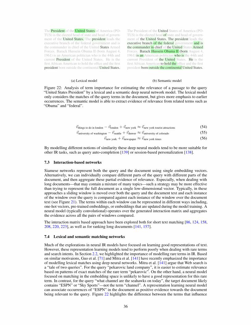
The President of the United States of America (PO-TUS) is the elected head of state and head of govern-ment of the United States. The president leads theexecutive branch of the federal government and isthe commander in chief of the United States ArmedForces. Barack Hussein Obama II (born August 4,1961) is an American politician who is the 44th andcurrent President of the United States. He is thefirst African American to hold the office and the firstpresident born outside the continental United States.

(a) Lexical model

The President of the United States of America (PO-TUS) is the elected head of state and head of govern-ment of the United States. The president leads theexecutive branch of the federal government and isthe commander in chief of the United States ArmedForces. Barack Hussein Obama II (born August 4,1961) is an American politician who is the 44th andcurrent President of the United States. He is thefirst African American to hold the office and the firstpresident born outside the continental United States.

(b) Semantic model

Figure 22: Analysis of term importance for estimating the relevance of a passage to the query“United States President” by a lexical and a semantic deep neural network model. The lexical modelonly considers the matches of the query terms in the document, but gives more emphasis to earlieroccurrences. The semantic model is able to extract evidence of relevance from related terms such as“Obama” and “federal”.

~vthings to do in london − ~vlondon + ~vnew york ≈ ~vnew york tourist attractions (54)~vuniversity of washington − ~vseattle + ~vdenver ≈ ~vuniversity of colorado (55)

~vnew york + ~vnewspaper ≈ ~vnew york times (56)

By modelling different notions of similarity these deep neural models tend to be more suitable forother IR tasks, such as query auto-completion [139] or session-based personalization [138].

7.3 Interaction-based networks

Siamese networks represent both the query and the document using single embedding vectors.Alternatively, we can individually compare different parts of the query with different parts of thedocument, and then aggregate these partial evidence of relevance. Especially, when dealing withlong documents—that may contain a mixture of many topics—such a strategy may be more effectivethan trying to represent the full document as a single low-dimensional vector. Typically, in theseapproaches a sliding window is moved over both the query and the document text and each instanceof the window over the query is compared against each instance of the window over the documenttext (see Figure 21). The terms within each window can be represented in different ways including,one-hot vectors, pre-trained embeddings, or embeddings that are updated during the model training. Aneural model (typically convolutional) operates over the generated interaction matrix and aggregatesthe evidence across all the pairs of windows compared.

The interaction matrix based approach have been explored both for short text matching [86, 124, 158,208, 220, 223], as well as for ranking long documents [141, 157].

7.4 Lexical and semantic matching networks

Much of the explorations in neural IR models have focused on learning good representations of text.However, these representation learning models tend to perform poorly when dealing with rare termsand search intents. In Section 2.2, we highlighted the importance of modelling rare terms in IR. Basedon similar motivaions, Guo et al. [71] and Mitra et al. [141] have recently emphasized the importanceof modelling lexical matches using deep neural networks. Mitra et al. [141] argue that Web search isa “tale of two queries”. For the query “pekarovic land company”, it is easier to estimate relevancebased on patterns of exact matches of the rare term “pekarovic”. On the other hand, a neural modelfocused on matching in the embedding space is unlikely to have a good representation for this rareterm. In contrast, for the query “what channel are the seahawks on today”, the target document likelycontains “ESPN” or “Sky Sports”—not the term “channel”. A representation learning neural modelcan associate occurrences of “ESPN” in the document as positive evidence towards the documentbeing relevant to the query. Figure 22 highlights the difference between the terms that influence

36

query text

generate query

term vector

doc text

generate doc

term vector

generate interaction matrix

query

term vector

doc

term vector

query text

generate query

embedding

doc text

generate doc

embedding

hadamard product

query

embedding

doc

embedding

fully connected layers for matching fully connected layers for matching

sum

lexical matching model semantic matching model

Figure 23: In the Duet architecture [141], the two sub-networks are jointly trained and the final outputis a linear combination of the outputs of the lexical and the semantic matching sub-networks. Thelexical matching sub-network (left) uses a convolutional model that operates over a binary interactionmatrix.16The semantic matching sub-network (right) learns representations of query and documenttext for effective matching in the embedding space. Cross-entropy loss is used to train the networksimilar to other models in Section 7.2.

the estimation of relevance of the same query-passage pair by a lexical matching and a semanticmatching model. A good neural IR model should incorporate both lexical and semantic matchingsignals [141].

Guo et al. [71] proposed to use histogram-based features in their DNN model to capture lexicalnotion of relevance. Mitra et al. [141] leverage large scale labelled data from Bing to train a Duetarchitecture (Figure 23) that learns to identify good patterns of both lexical and semantic matchesjointly. Neural models that focus on lexical matching typically have fewer parameters, and can betrained under small data regimes—unlike their counterparts that focus on learning representations oftext.

Interestingly, a query level analysis seems to indicate that both traditional non-neural IR approachesand more recent neural methods tend to perform well on different segments of queries depending onwhether they focus on lexical or semantic matching. Figure 24 plots a few of these models based ontheir per-query NDCG values on a test set.

8 Conclusion

We present a tutorial on neural methods for information retrieval. For machine learning researcherswho may be less familiar with IR tasks, we introduced the fundamentals of traditional IR modelsand metrics. For IR researchers, we summarized key concepts related to representation learningwith (shallow or deep) neural networks. Finally, we presented some of the recent neural methods fordocument ranking and question-answer matching.

16It is important to emphasize, that while Mitra et al. [141] and others have used interaction-based representa-tion for modelling lexical matches, the two ideas are distinct. Some interaction-matrix based representationscompare texts using their pre-trained embeddings [86, 223]. Similarly, lexical matching can be modelled withoutemploying an interaction matrix based representation [71].

37

●

BM25

●

QL

● DM

●

LSA

●

DSSM

●

CDSSM

●

DESM

● DRMM

●

Duet (Lexical) ●

Duet (Semantic)●Duet

Figure 24: A demonstration that IR models that focus on lexical matching tend to perform well onqueries that are distinct from queries on which semantic matching models achieve good relevance.Each model is represented by a vector of NDCG scores achieved on a set of test queries. Forvisualization, t-SNE [128] is used to plot the points in a two-dimensional space. Lexical matchingmodels (BM25, QL, DM, DRMM, and Duet-Lexical) are seen to form a cluster—as well as themodels that focus on representation learning.

We have focused on retrieval of long and short text. In the case of long text, the model must dealwith variable length documents, where the relevant sections of a document may be surrounded byirrelevant text. For both long and short text, but particularly for short, IR models should also dealwith the query-document vocabulary mismatch problem, by learning how patterns of query wordsand (different) document words can indicate relevance. Models should also consider lexical matcheswhen the query contains rare terms—such as a person’s name or a product model number—not seenduring training, and to avoid retrieving semantically related but irrelevant results.

An ideal model for information retrieval would be able to infer the meaning of a query from context.Given a query about the Prime Minister of UK, for example, it may be obvious from context whetherit refers to John Major or Teresa May—perhaps due to the time period of the corpus, or it may need tobe disambiguated based on other context such as the other query terms or the user’s short or long-termhistory. The ideal IR model may need to encode this context, which means that the model is likea library that effectively memorizes massive number of connections between entities and contexts.The number of learnable parameters of a ML model, however, is typically fixed, which may implythat there is a limited budget for how much real world knowledge the model can incorporate duringtraining. An ideal model, therefore, may also need to learn to be like a librarian with incompletedomain knowledge, but capable of reading documents related to the current query and reasoningabout the meaning of the query as part of the retrieval process.

Many of the breakthroughs in deep learning have been motivated by the needs of specific applicationareas. Convolutional neural networks, for example, are particularly popular with the vision community,whereas recurrent architectures find more applications in speech recognition and NLP. It is likely thatthe specific needs and challenges of IR tasks may motivate novel neural architectures and methods.Future IR explorations may also be motivated by developments in related areas, such as NLP. Forexample, neural architectures that have been evaluated on non-IR tasks [39, 50, 95, 99, 232] can beinvestigated in the retrieval context. Similarly, new methods for training deep models for NLP—e.g.,using reinforcement learning [163, 224] and generative adversarial networks (GANs) [226]—maycarry over to the IR setup.

However, given the pace at which the area of deep learning is growing, in terms of the number ofnew architectures and training regimes, we should be wary of the combinatorial explosion of tryingevery model on every IR task. We should not disproportionately focus on maximizing quantitativeimprovements and in the process neglect theoretical understanding and qualitative insights. It would

38

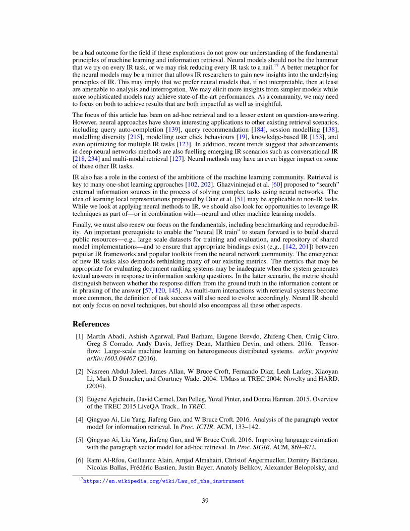
be a bad outcome for the field if these explorations do not grow our understanding of the fundamentalprinciples of machine learning and information retrieval. Neural models should not be the hammerthat we try on every IR task, or we may risk reducing every IR task to a nail.17 A better metaphor forthe neural models may be a mirror that allows IR researchers to gain new insights into the underlyingprinciples of IR. This may imply that we prefer neural models that, if not interpretable, then at leastare amenable to analysis and interrogation. We may elicit more insights from simpler models whilemore sophisticated models may achieve state-of-the-art performances. As a community, we may needto focus on both to achieve results that are both impactful as well as insightful.

The focus of this article has been on ad-hoc retrieval and to a lesser extent on question-answering.However, neural approaches have shown interesting applications to other existing retrieval scenarios,including query auto-completion [139], query recommendation [184], session modelling [138],modelling diversity [215], modelling user click behaviours [19], knowledge-based IR [153], andeven optimizing for multiple IR tasks [123]. In addition, recent trends suggest that advancementsin deep neural networks methods are also fuelling emerging IR scenarios such as conversational IR[218, 234] and multi-modal retrieval [127]. Neural methods may have an even bigger impact on someof these other IR tasks.

IR also has a role in the context of the ambitions of the machine learning community. Retrieval iskey to many one-shot learning approaches [102, 202]. Ghazvininejad et al. [60] proposed to “search”external information sources in the process of solving complex tasks using neural networks. Theidea of learning local representations proposed by Diaz et al. [51] may be applicable to non-IR tasks.While we look at applying neural methods to IR, we should also look for opportunities to leverage IRtechniques as part of—or in combination with—neural and other machine learning models.

Finally, we must also renew our focus on the fundamentals, including benchmarking and reproducibil-ity. An important prerequisite to enable the “neural IR train” to steam forward is to build sharedpublic resources—e.g., large scale datasets for training and evaluation, and repository of sharedmodel implementations—and to ensure that appropriate bindings exist (e.g., [142, 201]) betweenpopular IR frameworks and popular toolkits from the neural network community. The emergenceof new IR tasks also demands rethinking many of our existing metrics. The metrics that may beappropriate for evaluating document ranking systems may be inadequate when the system generatestextual answers in response to information seeking questions. In the latter scenario, the metric shoulddistinguish between whether the response differs from the ground truth in the information content orin phrasing of the answer [57, 120, 145]. As multi-turn interactions with retrieval systems becomemore common, the definition of task success will also need to evolve accordingly. Neural IR shouldnot only focus on novel techniques, but should also encompass all these other aspects.

References[1] Martín Abadi, Ashish Agarwal, Paul Barham, Eugene Brevdo, Zhifeng Chen, Craig Citro,

Greg S Corrado, Andy Davis, Jeffrey Dean, Matthieu Devin, and others. 2016. Tensor-flow: Large-scale machine learning on heterogeneous distributed systems. arXiv preprintarXiv:1603.04467 (2016).

[2] Nasreen Abdul-Jaleel, James Allan, W Bruce Croft, Fernando Diaz, Leah Larkey, XiaoyanLi, Mark D Smucker, and Courtney Wade. 2004. UMass at TREC 2004: Novelty and HARD.(2004).

[3] Eugene Agichtein, David Carmel, Dan Pelleg, Yuval Pinter, and Donna Harman. 2015. Overviewof the TREC 2015 LiveQA Track.. In TREC.

[4] Qingyao Ai, Liu Yang, Jiafeng Guo, and W Bruce Croft. 2016. Analysis of the paragraph vectormodel for information retrieval. In Proc. ICTIR. ACM, 133–142.

[5] Qingyao Ai, Liu Yang, Jiafeng Guo, and W Bruce Croft. 2016. Improving language estimationwith the paragraph vector model for ad-hoc retrieval. In Proc. SIGIR. ACM, 869–872.

[6] Rami Al-Rfou, Guillaume Alain, Amjad Almahairi, Christof Angermueller, Dzmitry Bahdanau,Nicolas Ballas, Frédéric Bastien, Justin Bayer, Anatoly Belikov, Alexander Belopolsky, and

17https://en.wikipedia.org/wiki/Law_of_the_instrument

39

others. 2016. Theano: A Python framework for fast computation of mathematical expressions.arXiv preprint arXiv:1605.02688 (2016).

[7] Sanjeev Arora, Yuanzhi Li, Yingyu Liang, Tengyu Ma, and Andrej Risteski. 2015. Rand-walk:A latent variable model approach to word embeddings. arXiv preprint arXiv:1502.03520(2015).

[8] Dzmitry Bahdanau, Kyunghyun Cho, and Yoshua Bengio. 2014. Neural machine translation byjointly learning to align and translate. arXiv preprint arXiv:1409.0473 (2014).

[9] Peter Bailey, Nick Craswell, and David Hawking. 2003. Engineering a multi-purpose testcollection for web retrieval experiments. Information Processing & Management 39, 6 (2003),853–871.

[10] Pierre Baldi and Yves Chauvin. 1993. Neural networks for fingerprint recognition. NeuralComputation 5, 3 (1993), 402–418.

[11] Marco Baroni, Georgiana Dinu, and Germán Kruszewski. 2014. Don’t count, predict! asystematic comparison of context-counting vs. context-predicting semantic vectors. In Proc.ACL, Vol. 1. 238–247.

[12] Marco Baroni and Alessandro Lenci. 2010. Distributional memory: A general framework forcorpus-based semantics. Computational Linguistics 36, 4 (2010), 673–721.

[13] Roland Barthes. 1977. Elements of semiology. Macmillan.

[14] Yoshua Bengio and others. 2009. Learning deep architectures for AI. Foundations and trends R©in Machine Learning 2, 1 (2009), 1–127.

[15] Yoshua Bengio, Réjean Ducharme, Pascal Vincent, and Christian Jauvin. 2003. A neuralprobabilistic language model. Journal of machine learning research 3, Feb (2003), 1137–1155.

[16] Yoshua Bengio, Pascal Lamblin, Dan Popovici, Hugo Larochelle, and others. 2007. Greedylayer-wise training of deep networks. Proc. NIPS 19 (2007), 153.

[17] Adam Berger and John Lafferty. 1999. Information retrieval as statistical translation. In Proc.SIGIR. ACM, 222–229.

[18] Antoine Bordes, Nicolas Usunier, Sumit Chopra, and Jason Weston. 2015. Large-scale simplequestion answering with memory networks. arXiv preprint arXiv:1506.02075 (2015).

[19] Alexey Borisov, Ilya Markov, Maarten de Rijke, and Pavel Serdyukov. 2016. A neural clickmodel for web search. In Proc. WWW. Proc. WWW, 531–541.

[20] Samuel R Bowman, Jon Gauthier, Abhinav Rastogi, Raghav Gupta, Christopher D Manning,and Christopher Potts. 2016. A fast unified model for parsing and sentence understanding. arXivpreprint arXiv:1603.06021 (2016).

[21] Jane Bromley, James W. Bentz, Léon Bottou, Isabelle Guyon, Yann LeCun, Cliff Moore, EduardSäckinger, and Roopak Shah. 1993. Signature Verification Using A "Siamese" Time DelayNeural Network. IJPRAI 7, 4 (1993), 669–688.

[22] Peter F Brown, John Cocke, Stephen A Della Pietra, Vincent J Della Pietra, Fredrick Jelinek,John D Lafferty, Robert L Mercer, and Paul S Roossin. 1990. A statistical approach to machinetranslation. Computational linguistics 16, 2 (1990), 79–85.

[23] Peter F Brown, Vincent J Della Pietra, Stephen A Della Pietra, and Robert L Mercer. 1993. Themathematics of statistical machine translation: Parameter estimation. Computational linguistics19, 2 (1993), 263–311.

[24] John A Bullinaria and Joseph P Levy. 2007. Extracting semantic representations from wordco-occurrence statistics: A computational study. Behavior research methods 39, 3 (2007),510–526.

40

[25] John A Bullinaria and Joseph P Levy. 2012. Extracting semantic representations from wordco-occurrence statistics: stop-lists, stemming, and SVD. Behavior research methods 44, 3(2012), 890–907.

[26] Chris Burges, Tal Shaked, Erin Renshaw, Ari Lazier, Matt Deeds, Nicole Hamilton, andGreg Hullender. 2005. Learning to rank using gradient descent. In Proceedings of the 22ndinternational conference on Machine learning. ACM, 89–96.

[27] Christopher JC Burges. 2010. From ranknet to lambdarank to lambdamart: An overview.Learning 11, 23-581 (2010), 81.

[28] Christopher JC Burges, Robert Ragno, and Quoc Viet Le. 2006. Learning to rank with nons-mooth cost functions. In NIPS, Vol. 6. 193–200.

[29] Jamie Callan, Mark Hoy, Changkuk Yoo, and Le Zhao. 2009. Clueweb09 data set. (2009).

[30] Daniel Chandler. 1994. Semiotics for beginners. (1994).

[31] Tianqi Chen, Mu Li, Yutian Li, Min Lin, Naiyan Wang, Minjie Wang, Tianjun Xiao, Bing Xu,Chiyuan Zhang, and Zheng Zhang. 2015. Mxnet: A flexible and efficient machine learninglibrary for heterogeneous distributed systems. arXiv preprint arXiv:1512.01274 (2015).

[32] Kyunghyun Cho, Bart Van Merriënboer, Dzmitry Bahdanau, and Yoshua Bengio. 2014. Onthe properties of neural machine translation: Encoder-decoder approaches. arXiv preprintarXiv:1409.1259 (2014).

[33] Jan K Chorowski, Dzmitry Bahdanau, Dmitriy Serdyuk, Kyunghyun Cho, and Yoshua Bengio.2015. Attention-based models for speech recognition. In Proc. NIPS. 577–585.

[34] Junyoung Chung, Caglar Gulcehre, KyungHyun Cho, and Yoshua Bengio. 2014. Empir-ical evaluation of gated recurrent neural networks on sequence modeling. arXiv preprintarXiv:1412.3555 (2014).

[35] Stéphane Clinchant and Florent Perronnin. 2013. Aggregating continuous word embeddings forinformation retrieval. In Proceedings of the Workshop on Continuous Vector Space Models andtheir Compositionality. 100–109.

[36] Daniel Cohen, Qingyao Ai, and W Bruce Croft. 2016. Adaptability of neural networks onvarying granularity ir tasks. arXiv preprint arXiv:1606.07565 (2016).

[37] Daniel Cohen and W Bruce Croft. 2016. End to End Long Short Term Memory Networks forNon-Factoid Question Answering. In Proc. ICTIR. ACM, 143–146.

[38] Ronan Collobert, Koray Kavukcuoglu, and Clément Farabet. 2011. Torch7: A matlab-likeenvironment for machine learning. In BigLearn, NIPS Workshop.

[39] Ronan Collobert, Jason Weston, Léon Bottou, Michael Karlen, Koray Kavukcuoglu, and PavelKuksa. 2011. Natural language processing (almost) from scratch. The Journal of MachineLearning Research 12 (2011), 2493–2537.

[40] Nick Craswell. 2009. Mean reciprocal rank. In Encyclopedia of Database Systems. Springer,1703–1703.

[41] Nick Craswell. 2017. Neural Models for Full Text Search. In Proceedings of the Tenth ACMInternational Conference on Web Search and Data Mining. ACM, 251–251.

[42] Nick Craswell, W Bruce Croft, Maarten de Rijke, Jiafeng Guo, and Bhaskar Mitra. 2017.Neu-IR’17: Neural Information Retrieval. In Proc. SIGIR. ACM.

[43] Nick Craswell, W Bruce Croft, Jiafeng Guo, Bhaskar Mitra, and Maarten de Rijke. 2016.Neu-IR: The SIGIR 2016 Workshop on Neural Information Retrieval. (2016).

[44] Nick Craswell, W Bruce Croft, Jiafeng Guo, Bhaskar Mitra, and Maarten de Rijke. 2016. Reporton the SIGIR 2016 Workshop on Neural Information Retrieval (Neu-IR). ACM Sigir forum 50,2 (2016), 96–103.

41

[45] Nick Craswell, David Hawking, Ross Wilkinson, and Mingfang Wu. 2003. Overview of theTREC 2002 Web track. In TREC, Vol. 3. 12th.

[46] Nick Craswell, Rosie Jones, Georges Dupret, and Evelyne Viegas. 2009. Proceedings of the2009 workshop on Web Search Click Data. ACM.

[47] Ferdinand De Saussure, Wade Baskin, and Perry Meisel. 2011. Course in general linguistics.Columbia University Press.

[48] Scott C. Deerwester, Susan T Dumais, Thomas K. Landauer, George W. Furnas, and Richard A.Harshman. 1990. Indexing by latent semantic analysis. JASIS 41, 6 (1990), 391–407.

[49] Li Deng, Dong Yu, and others. 2014. Deep learning: methods and applications. Foundationsand Trends R© in Signal Processing 7, 3–4 (2014), 197–387.

[50] Misha Denil, Alban Demiraj, Nal Kalchbrenner, Phil Blunsom, and Nando de Freitas. 2014.Modelling, visualising and summarising documents with a single convolutional neural network.arXiv preprint arXiv:1406.3830 (2014).

[51] Fernando Diaz, Bhaskar Mitra, and Nick Craswell. 2016. Query Expansion with Locally-TrainedWord Embeddings. In Proc. ACL.

[52] Fernando Diaz, Ryen White, Georg Buscher, and Dan Liebling. 2013. Robust models of mousemovement on dynamic web search results pages. In Proceedings of the 22nd ACM internationalconference on Conference on information & knowledge management. ACM, 1451–1460.

[53] John Duchi, Elad Hazan, and Yoram Singer. 2011. Adaptive subgradient methods for onlinelearning and stochastic optimization. Journal of Machine Learning Research 12, Jul (2011),2121–2159.

[54] Jeffrey L Elman. 1990. Finding structure in time. Cognitive science 14, 2 (1990), 179–211.

[55] David Ferrucci, Eric Brown, Jennifer Chu-Carroll, James Fan, David Gondek, Aditya AKalyanpur, Adam Lally, J William Murdock, Eric Nyberg, John Prager, and others. 2010.Building Watson: An overview of the DeepQA project. AI magazine 31, 3 (2010), 59–79.

[56] John R Firth. 1957. A synopsis of linguistic theory, 1930-1955. (1957).

[57] Michel Galley, Chris Brockett, Alessandro Sordoni, Yangfeng Ji, Michael Auli, Chris Quirk,Margaret Mitchell, Jianfeng Gao, and Bill Dolan. 2015. deltaBLEU: A discriminative metricfor generation tasks with intrinsically diverse targets. arXiv preprint arXiv:1506.06863 (2015).

[58] Debasis Ganguly, Dwaipayan Roy, Mandar Mitra, and Gareth JF Jones. 2015. Word Embeddingbased Generalized Language Model for Information Retrieval. In Proc. SIGIR. ACM, 795–798.

[59] Jianfeng Gao, Patrick Pantel, Michael Gamon, Xiaodong He, Li Deng, and Yelong Shen. 2014.Modeling interestingness with deep neural networks. In Proceedings of the 2013 Conference onEmpirical Methods in Natural Language Processing.

[60] Marjan Ghazvininejad, Chris Brockett, Ming-Wei Chang, Bill Dolan, Jianfeng Gao, Wen-tauYih, and Michel Galley. 2017. A Knowledge-Grounded Neural Conversation Model. arXivpreprint arXiv:1702.01932 (2017).

[61] Yoav Goldberg and Omer Levy. 2014. word2vec Explained: deriving Mikolov et al.’s negative-sampling word-embedding method. arXiv preprint arXiv:1402.3722 (2014).

[62] Christoph Goller and Andreas Kuchler. 1996. Learning task-dependent distributed represen-tations by backpropagation through structure. In Neural Networks, 1996., IEEE InternationalConference on, Vol. 1. IEEE, 347–352.

[63] Gene H Golub and Christian Reinsch. 1970. Singular value decomposition and least squaressolutions. Numerische mathematik 14, 5 (1970), 403–420.

[64] Ian Goodfellow, Yoshua Bengio, and Aaron Courville. 2016. Deep learning. MIT Press.

42

[65] Laura A Granka, Thorsten Joachims, and Geri Gay. 2004. Eye-tracking analysis of user behaviorin WWW search. In Proceedings of the 27th annual international ACM SIGIR conference onResearch and development in information retrieval. ACM, 478–479.

[66] Alex Graves. 2013. Generating sequences with recurrent neural networks. arXiv preprintarXiv:1308.0850 (2013).

[67] Alex Graves, Marcus Liwicki, Santiago Fernández, Roman Bertolami, Horst Bunke, and JürgenSchmidhuber. 2009. A novel connectionist system for unconstrained handwriting recognition.IEEE transactions on pattern analysis and machine intelligence 31, 5 (2009), 855–868.

[68] Mihajlo Grbovic, Nemanja Djuric, Vladan Radosavljevic, and Narayan Bhamidipati. 2015.Search Retargeting using Directed Query Embeddings. In Proc. WWW. International WorldWide Web Conferences Steering Committee, 37–38.

[69] Mihajlo Grbovic, Nemanja Djuric, Vladan Radosavljevic, Fabrizio Silvestri, and NarayanBhamidipati. 2015. Context-and Content-aware Embeddings for Query Rewriting in SponsoredSearch. In Proc. SIGIR. ACM, 383–392.

[70] Zhiwei Guan and Edward Cutrell. 2007. An eye tracking study of the effect of target rank onweb search. In Proceedings of the SIGCHI conference on Human factors in computing systems.ACM, 417–420.

[71] Jiafeng Guo, Yixing Fan, Qingyao Ai, and W Bruce Croft. 2016. A Deep Relevance MatchingModel for Ad-hoc Retrieval. In Proc. CIKM. ACM, 55–64.

[72] Jiafeng Guo, Yixing Fan, Qingyao Ai, and W Bruce Croft. 2016. Semantic Matching byNon-Linear Word Transportation for Information Retrieval. In Proc. CIKM. ACM, 701–710.

[73] Richard HR Hahnloser, Rahul Sarpeshkar, Misha A Mahowald, Rodney J Douglas, and H Se-bastian Seung. 2000. Digital selection and analogue amplification coexist in a cortex-inspiredsilicon circuit. Nature 405, 6789 (2000), 947–951.

[74] Roy Harris. 2001. Saussure and his Interpreters. Edinburgh University Press.

[75] Zellig S Harris. 1954. Distributional structure. Word 10, 2-3 (1954), 146–162.

[76] Kaiming He, Xiangyu Zhang, Shaoqing Ren, and Jian Sun. 2016. Deep residual learning forimage recognition. In Proceedings of the IEEE Conference on Computer Vision and PatternRecognition. 770–778.

[77] Robert Hecht-Nielsen and others. 1988. Theory of the backpropagation neural network. NeuralNetworks 1, Supplement-1 (1988), 445–448.

[78] Karl Moritz Hermann, Tomas Kocisky, Edward Grefenstette, Lasse Espeholt, Will Kay, MustafaSuleyman, and Phil Blunsom. 2015. Teaching machines to read and comprehend. In Proc. NIPS.1693–1701.

[79] Djoerd Hiemstra. 2001. Using language models for information retrieval. Taaluitgeverij NesliaPaniculata.

[80] Felix Hill, Antoine Bordes, Sumit Chopra, and Jason Weston. 2015. The Goldilocks Prin-ciple: Reading Children’s Books with Explicit Memory Representations. arXiv preprintarXiv:1511.02301 (2015).

[81] Geoffrey Hinton, Li Deng, Dong Yu, George E Dahl, Abdel-rahman Mohamed, Navdeep Jaitly,Andrew Senior, Vincent Vanhoucke, Patrick Nguyen, Tara N Sainath, and others. 2012. Deepneural networks for acoustic modeling in speech recognition: The shared views of four researchgroups. Signal Processing Magazine, IEEE 29, 6 (2012), 82–97.

[82] Geoffrey E Hinton. 1984. Distributed representations. (1984).

[83] Sepp Hochreiter and Jürgen Schmidhuber. 1997. Long short-term memory. Neural computation9, 8 (1997), 1735–1780.

43

[84] Kajta Hofmann, Bhaskar Mitra, Filip Radlinski, and Milad Shokouhi. 2014. An Eye-trackingStudy of User Interactions with Query Auto Completion. In Proc. CIKM. ACM, 549–558.

[85] Kurt Hornik, Maxwell Stinchcombe, and Halbert White. 1989. Multilayer feedforward networksare universal approximators. Neural networks 2, 5 (1989), 359–366.

[86] Baotian Hu, Zhengdong Lu, Hang Li, and Qingcai Chen. 2014. Convolutional neural networkarchitectures for matching natural language sentences. In Proc. NIPS. 2042–2050.

[87] Gao Huang, Chuan Guo, Matt J Kusner, Yu Sun, Fei Sha, and Kilian Q Weinberger. 2016.Supervised Word Mover’s Distance. In Proc. NIPS. 4862–4870.

[88] Po-Sen Huang, Xiaodong He, Jianfeng Gao, Li Deng, Alex Acero, and Larry Heck. 2013.Learning deep structured semantic models for web search using clickthrough data. In Proc.CIKM. ACM, 2333–2338.

[89] Kevin Jarrett, Koray Kavukcuoglu, Yann LeCun, and others. 2009. What is the best multi-stage architecture for object recognition?. In Computer Vision, 2009 IEEE 12th InternationalConference on. IEEE, 2146–2153.

[90] Kalervo Järvelin and Jaana Kekäläinen. 2002. Cumulated gain-based evaluation of IR techniques.ACM Transactions on Information Systems (TOIS) 20, 4 (2002), 422–446.

[91] Yangqing Jia, Evan Shelhamer, Jeff Donahue, Sergey Karayev, Jonathan Long, Ross Girshick,Sergio Guadarrama, and Trevor Darrell. 2014. Caffe: Convolutional architecture for fast featureembedding. In Proceedings of the 22nd ACM international conference on Multimedia. ACM,675–678.

[92] Thorsten Joachims, Laura Granka, Bing Pan, Helene Hembrooke, and Geri Gay. 2005. Accu-rately interpreting clickthrough data as implicit feedback. In Proceedings of the 28th annualinternational ACM SIGIR conference on Research and development in information retrieval.Acm, 154–161.

[93] Thorsten Joachims, Laura Granka, Bing Pan, Helene Hembrooke, Filip Radlinski, and Geri Gay.2007. Evaluating the accuracy of implicit feedback from clicks and query reformulations inweb search. ACM Transactions on Information Systems (TOIS) 25, 2 (2007), 7.

[94] Rafal Jozefowicz, Oriol Vinyals, Mike Schuster, Noam Shazeer, and Yonghui Wu. 2016.Exploring the limits of language modeling. arXiv preprint arXiv:1602.02410 (2016).

[95] Nal Kalchbrenner, Edward Grefenstette, and Phil Blunsom. 2014. A convolutional neuralnetwork for modelling sentences. arXiv preprint arXiv:1404.2188 (2014).

[96] Tom Kenter, Alexey Borisov, and Maarten de Rijke. 2016. Siamese cbow: Optimizing wordembeddings for sentence representations. arXiv preprint arXiv:1606.04640 (2016).

[97] Tom Kenter, Alexey Borisov, Christophe Van Gysel, Mostafa Dehghani, Maarten de Rijke, andBhaskar Mitra. 2017. Neural Networks for Information Retrieval (NN4IR). In Proc. SIGIR.ACM.

[98] Tom Kenter and Maarten de Rijke. Short Text Similarity with Word Embeddings. In Proc.CIKM, Vol. 15. 115.

[99] Yoon Kim. 2014. Convolutional neural networks for sentence classification. arXiv preprintarXiv:1408.5882 (2014).

[100] Yoon Kim, Yacine Jernite, David Sontag, and Alexander M Rush. 2015. Character-awareneural language models. arXiv preprint arXiv:1508.06615 (2015).

[101] Ryan Kiros, Richard Zemel, and Ruslan R Salakhutdinov. 2014. A multiplicative model forlearning distributed text-based attribute representations. In Proc. NIPS. 2348–2356.

[102] Gregory Koch. 2015. Siamese neural networks for one-shot image recognition. Ph.D. Disser-tation. University of Toronto.

44

[103] Alex Krizhevsky, Ilya Sutskever, and Geoffrey E Hinton. 2012. Imagenet classification withdeep convolutional neural networks. In Proc. NIPS. 1097–1105.

[104] Matt J Kusner, EDU Yu Sun, EDU Nicholas I Kolkin, and WUSTL EDU. From WordEmbeddings To Document Distances. (????).

[105] John Lafferty and Chengxiang Zhai. 2001. Document language models, query models, andrisk minimization for information retrieval. In Proceedings of the 24th annual internationalACM SIGIR conference on Research and development in information retrieval. ACM, 111–119.

[106] Dmitry Lagun, Chih-Hung Hsieh, Dale Webster, and Vidhya Navalpakkam. 2014. Towardsbetter measurement of attention and satisfaction in mobile search. In Proceedings of the 37thinternational ACM SIGIR conference on Research & development in information retrieval.ACM, 113–122.

[107] Gustav Larsson, Michael Maire, and Gregory Shakhnarovich. 2016. Fractalnet: Ultra-deepneural networks without residuals. arXiv preprint arXiv:1605.07648 (2016).

[108] Victor Lavrenko. 2008. A generative theory of relevance. Vol. 26. Springer Science & BusinessMedia.

[109] Victor Lavrenko and W Bruce Croft. 2001. Relevance based language models. In Proceedingsof the 24th annual international ACM SIGIR conference on Research and development ininformation retrieval. ACM, 120–127.

[110] Quoc V Le and Tomas Mikolov. 2014. Distributed Representations of Sentences and Docu-ments.. In ICML, Vol. 14. 1188–1196.

[111] Rémi Lebret and Ronan Collobert. 2013. Word emdeddings through hellinger PCA. arXivpreprint arXiv:1312.5542 (2013).

[112] Yann LeCun, Yoshua Bengio, and Geoffrey Hinton. 2015. Deep learning. Nature 521, 7553(2015), 436–444.

[113] Yann LeCun, Fu Jie Huang, and Leon Bottou. 2004. Learning methods for generic objectrecognition with invariance to pose and lighting. In Computer Vision and Pattern Recognition,2004. CVPR 2004. Proceedings of the 2004 IEEE Computer Society Conference on, Vol. 2.IEEE, II–104.

[114] Yann LeCun, Koray Kavukcuoglu, and Clément Farabet. 2010. Convolutional networks andapplications in vision. In Circuits and Systems (ISCAS), Proceedings of 2010 IEEE InternationalSymposium on. IEEE, 253–256.

[115] Omer Levy and Yoav Goldberg. 2014. Dependencybased word embeddings. In Proc. ACL,Vol. 2. 302–308.

[116] Omer Levy, Yoav Goldberg, and Ido Dagan. 2015. Improving distributional similarity withlessons learned from word embeddings. Transactions of the Association for ComputationalLinguistics 3 (2015), 211–225.

[117] Omer Levy, Yoav Goldberg, and Israel Ramat-Gan. 2014. Linguistic regularities in sparse andexplicit word representations. CoNLL-2014 (2014), 171.

[118] Steven Levy. 2011. In the plex: How Google thinks, works, and shapes our lives. Simon andSchuster.

[119] Hang Li and Zhengdong Lu. Deep Learning for Information Retrieval. (????).

[120] Chia-Wei Liu, Ryan Lowe, Iulian V Serban, Michael Noseworthy, Laurent Charlin, and JoellePineau. 2016. How NOT to evaluate your dialogue system: An empirical study of unsupervisedevaluation metrics for dialogue response generation. arXiv preprint arXiv:1603.08023 (2016).

[121] Tie-Yan Liu. 2009. Learning to Rank for Information Retrieval. Foundation and Trends inInformation Retrieval 3, 3 (March 2009), 225–331.

45

[122] Tie-Yan Liu, Jun Xu, Tao Qin, Wenying Xiong, and Hang Li. 2007. Letor: Benchmarkdataset for research on learning to rank for information retrieval. In Proceedings of SIGIR 2007workshop on learning to rank for information retrieval. 3–10.

[123] Xiaodong Liu, Jianfeng Gao, Xiaodong He, Li Deng, Kevin Duh, and Ye-Yi Wang. Repre-sentation Learning Using Multi-Task Deep Neural Networks for Semantic Classification andInformation Retrieval. Proc. NAACL, May 2015 (????).

[124] Zhengdong Lu and Hang Li. 2013. A deep architecture for matching short texts. In Proc. NIPS.1367–1375.

[125] Kevin Lund and Curt Burgess. 1996. Producing high-dimensional semantic spaces from lexicalco-occurrence. Behavior Research Methods, Instruments, & Computers 28, 2 (1996), 203–208.

[126] Minh-Thang Luong, Hieu Pham, and Christopher D Manning. 2015. Effective approaches toattention-based neural machine translation. arXiv preprint arXiv:1508.04025 (2015).

[127] Lin Ma, Zhengdong Lu, Lifeng Shang, and Hang Li. 2015. Multimodal convolutional neuralnetworks for matching image and sentence. In Proceedings of the IEEE International Conferenceon Computer Vision. 2623–2631.

[128] Laurens van der Maaten and Geoffrey Hinton. 2008. Visualizing data using t-SNE. Journal ofMachine Learning Research 9, Nov (2008), 2579–2605.

[129] Christopher Manning. 2016. Understanding Human Language: Can NLP and Deep LearningHelp?. In Proc. SIGIR. ACM, 1–1.

[130] Ivan Markovsky. 2011. Low rank approximation: algorithms, implementation, applications.Springer Science & Business Media.

[131] Irina Matveeva, Chris Burges, Timo Burkard, Andy Laucius, and Leon Wong. 2006. Highaccuracy retrieval with multiple nested ranker. In Proceedings of the 29th annual internationalACM SIGIR conference on Research and development in information retrieval. ACM, 437–444.

[132] Donald Metzler and W Bruce Croft. 2005. A Markov random field model for term dependen-cies. In Proc. SIGIR. ACM, 472–479.

[133] Donald Metzler, Susan Dumais, and Christopher Meek. 2007. Similarity measures for shortsegments of text. In European Conference on Information Retrieval. Springer, 16–27.

[134] Tomas Mikolov, Kai Chen, Greg Corrado, and Jeffrey Dean. 2013. Efficient estimation ofword representations in vector space. arXiv preprint arXiv:1301.3781 (2013).

[135] Tomas Mikolov, Martin Karafiát, Lukas Burget, Jan Cernocky, and Sanjeev Khudanpur. 2010.Recurrent neural network based language model.. In Interspeech, Vol. 2. 3.

[136] Tomas Mikolov, Ilya Sutskever, Kai Chen, Greg S Corrado, and Jeff Dean. 2013. Distributedrepresentations of words and phrases and their compositionality. In Proc. NIPS. 3111–3119.

[137] Tomas Mikolov, Wen-tau Yih, and Geoffrey Zweig. 2013. Linguistic Regularities in ContinuousSpace Word Representations.. In HLT-NAACL. Citeseer, 746–751.

[138] Bhaskar Mitra. 2015. Exploring Session Context using Distributed Representations of Queriesand Reformulations. In Proc. SIGIR. ACM, 3–12.

[139] Bhaskar Mitra and Nick Craswell. 2015. Query Auto-Completion for Rare Prefixes. In Proc.CIKM. ACM.

[140] Bhaskar Mitra and Nick Craswell. 2017. Neural Text Embeddings for Information Retrieval.In Proc. WSDM. ACM, 813–814.

[141] Bhaskar Mitra, Fernando Diaz, and Nick Craswell. 2017. Learning to Match Using Local andDistributed Representations of Text for Web Search. In Proc. WWW. 1291–1299.

46

[142] Bhaskar Mitra, Fernando Diaz, and Nick Craswell. 2017. Luandri: a Clean Lua Interface tothe Indri Search Engine. In Proc. SIGIR. ACM.

[143] Bhaskar Mitra, Eric Nalisnick, Nick Craswell, and Rich Caruana. 2016. A Dual EmbeddingSpace Model for Document Ranking. arXiv preprint arXiv:1602.01137 (2016).

[144] Bhaskar Mitra, Milad Shokouhi, Filip Radlinski, and Katja Hofmann. 2014. On User Interac-tions with Query Auto-Completion. In Proc. SIGIR. 1055–1058.

[145] Bhaskar Mitra, Grady Simon, Jianfeng Gao, Nick Craswell, and Li Deng. 2016. A Proposalfor Evaluating Answer Distillation from Web Data. In Proceedings of the SIGIR 2016 WebQAWorkshop.

[146] Volodymyr Mnih, Nicolas Heess, Alex Graves, and others. 2014. Recurrent models of visualattention. In Proc. NIPS. 2204–2212.

[147] Volodymyr Mnih, Koray Kavukcuoglu, David Silver, Andrei A Rusu, Joel Veness, Marc GBellemare, Alex Graves, Martin Riedmiller, Andreas K Fidjeland, Georg Ostrovski, and others.2015. Human-level control through deep reinforcement learning. Nature 518, 7540 (2015),529–533.

[148] Guido F Montufar, Razvan Pascanu, Kyunghyun Cho, and Yoshua Bengio. 2014. On thenumber of linear regions of deep neural networks. In Proc. NIPS. 2924–2932.

[149] Frederic Morin and Yoshua Bengio. 2005. Hierarchical Probabilistic Neural Network LanguageModel.. In Aistats, Vol. 5. Citeseer, 246–252.

[150] Vinod Nair and Geoffrey E Hinton. 2010. Rectified linear units improve restricted boltzmannmachines. In Proc. ICML. 807–814.

[151] Eric Nalisnick, Bhaskar Mitra, Nick Craswell, and Rich Caruana. 2016. Improving DocumentRanking with Dual Word Embeddings. In Proc. WWW.

[152] Graham Neubig, Chris Dyer, Yoav Goldberg, Austin Matthews, Waleed Ammar, AntoniosAnastasopoulos, Miguel Ballesteros, David Chiang, Daniel Clothiaux, Trevor Cohn, and others.2017. DyNet: The Dynamic Neural Network Toolkit. arXiv preprint arXiv:1701.03980 (2017).

[153] Gia-Hung Nguyen, Lynda Tamine, Laure Soulier, and Nathalie Bricon-Souf. 2016. Toward adeep neural approach for knowledge-based ir. arXiv preprint arXiv:1606.07211 (2016).

[154] Tri Nguyen, Mir Rosenberg, Xia Song, Jianfeng Gao, Saurabh Tiwary, Rangan Majumder, andLi Deng. 2016. MS MARCO: A Human Generated MAchine Reading COmprehension Dataset.arXiv preprint arXiv:1611.09268 (2016).

[155] H Palangi, L Deng, Y Shen, J Gao, X He, J Chen, X Song, and R Ward. 2014. Seman-tic Modelling with Long-Short-Term Memory for Information Retrieval. arXiv preprintarXiv:1412.6629 (2014).

[156] Hamid Palangi, Li Deng, Yelong Shen, Jianfeng Gao, Xiaodong He, Jianshu Chen, XinyingSong, and Rabab Ward. 2015. Deep Sentence Embedding Using the Long Short Term MemoryNetwork: Analysis and Application to Information Retrieval. arXiv preprint arXiv:1502.06922(2015).

[157] Liang Pang, Yanyan Lan, Jiafeng Guo, Jun Xu, and Xueqi Cheng. 2016. A study of match-pyramid models on ad-hoc retrieval. arXiv preprint arXiv:1606.04648 (2016).

[158] Liang Pang, Yanyan Lan, Jiafeng Guo, Jun Xu, Shengxian Wan, and Xueqi Cheng. 2016. TextMatching as Image Recognition. In Proc. AAAI.

[159] Greg Pass, Abdur Chowdhury, and Cayley Torgeson. 2006. A picture of search. In Proc.InfoScale. ACM.

[160] Jeffrey Pennington, Richard Socher, and Christopher D Manning. 2014. Glove: Global vectorsfor word representation. Proc. EMNLP 12 (2014), 1532–1543.

47

[161] Jay M Ponte and W Bruce Croft. 1998. A language modeling approach to information retrieval.In Proc. SIGIR. ACM, 275–281.

[162] Pranav Rajpurkar, Jian Zhang, Konstantin Lopyrev, and Percy Liang. 2016. Squad: 100,000+questions for machine comprehension of text. arXiv preprint arXiv:1606.05250 (2016).

[163] Marc’Aurelio Ranzato, Sumit Chopra, Michael Auli, and Wojciech Zaremba. 2015. Sequencelevel training with recurrent neural networks. arXiv preprint arXiv:1511.06732 (2015).

[164] Marc’Aurelio Ranzato, Christopher Poultney, Sumit Chopra, and Yann LeCun. 2006. Efficientlearning of sparse representations with an energy-based model. In Proceedings of the 19thInternational Conference on Neural Information Processing Systems. MIT Press, 1137–1144.

[165] Matthew Richardson, Christopher JC Burges, and Erin Renshaw. 2013. MCTest: A ChallengeDataset for the Open-Domain Machine Comprehension of Text.. In EMNLP, Vol. 3. 4.

[166] Stephen Robertson, Hugo Zaragoza, and others. 2009. The probabilistic relevance framework:BM25 and beyond. Foundations and Trends R© in Information Retrieval 3, 4 (2009), 333–389.

[167] Stephen E Robertson, Evangelos Kanoulas, and Emine Yilmaz. 2010. Extending averageprecision to graded relevance judgments. In Proceedings of the 33rd international ACM SIGIRconference on Research and development in information retrieval. ACM, 603–610.

[168] Douglas LT Rohde, Laura M Gonnerman, and David C Plaut. 2006. An improved model ofsemantic similarity based on lexical co-occurrence. Commun. ACM 8 (2006), 627–633.

[169] Xin Rong. 2014. word2vec Parameter Learning Explained. arXiv preprint arXiv:1411.2738(2014).

[170] Dwaipayan Roy, Debjyoti Paul, Mandar Mitra, and Utpal Garain. 2016. Using Word Embed-dings for Automatic Query Expansion. arXiv preprint arXiv:1606.07608 (2016).

[171] Yossi Rubner, Carlo Tomasi, and Leonidas J Guibas. 1998. A metric for distributions withapplications to image databases. In Computer Vision, 1998. Sixth International Conference on.IEEE, 59–66.

[172] Magnus Sahlgren. 2006. The Word-Space Model: Using distributional analysis to representsyntagmatic and paradigmatic relations between words in high-dimensional vector spaces.Ph.D. Dissertation. Institutionen för lingvistik.

[173] Hasim Sak, Andrew W Senior, and Françoise Beaufays. 2014. Long short-term memoryrecurrent neural network architectures for large scale acoustic modeling.. In Interspeech. 338–342.

[174] Ruslan Salakhutdinov and Geoffrey Hinton. 2009. Semantic hashing. International Journal ofApproximate Reasoning 50, 7 (2009), 969–978.

[175] Jürgen Schmidhuber. 2015. Deep learning in neural networks: An overview. Neural networks61 (2015), 85–117.

[176] Aliaksei Severyn and Alessandro Moschitti. 2015. Learning to rank short text pairs withconvolutional deep neural networks. In Proc. SIGIR. ACM, 373–382.

[177] Yelong Shen, Xiaodong He, Jianfeng Gao, Li Deng, and Gregoire Mesnil. 2014. A latentsemantic model with convolutional-pooling structure for information retrieval. In Proc. CIKM.ACM, 101–110.

[178] Yelong Shen, Xiaodong He, Jianfeng Gao, Li Deng, and Grégoire Mesnil. 2014. Learningsemantic representations using convolutional neural networks for Web search. In Proc. WWW.373–374.

[179] Shaohuai Shi, Qiang Wang, Pengfei Xu, and Xiaowen Chu. 2016. Benchmarking State-of-the-Art Deep Learning Software Tools. arXiv preprint arXiv:1608.07249 (2016).

48

[180] David Silver, Aja Huang, Chris J Maddison, Arthur Guez, Laurent Sifre, George VanDen Driessche, Julian Schrittwieser, Ioannis Antonoglou, Veda Panneershelvam, Marc Lanctot,and others. 2016. Mastering the game of Go with deep neural networks and tree search. Nature529, 7587 (2016), 484–489.

[181] Amit Singhal, Chris Buckley, and Mandar Mitra. 1996. Pivoted document length normalization.In Proc. SIGIR. ACM, 21–29.

[182] Richard Socher, Cliff C Lin, Chris Manning, and Andrew Y Ng. 2011. Parsing natural scenesand natural language with recursive neural networks. In Proceedings of the 28th internationalconference on machine learning (ICML-11). 129–136.

[183] Richard Socher, Jeffrey Pennington, Eric H Huang, Andrew Y Ng, and Christopher D Manning.2011. Semi-supervised recursive autoencoders for predicting sentiment distributions. In Pro-ceedings of the conference on empirical methods in natural language processing. Associationfor Computational Linguistics, 151–161.

[184] Alessandro Sordoni, Yoshua Bengio, Hossein Vahabi, Christina Lioma, Jakob G Simonsen, andJian-Yun Nie. 2015. A Hierarchical Recurrent Encoder-Decoder for Generative Context-AwareQuery Suggestion. arXiv preprint arXiv:1507.02221 (2015).

[185] Alessandro Sordoni, Michel Galley, Michael Auli, Chris Brockett, Yangfeng Ji, MargaretMitchell, Jian-Yun Nie, Jianfeng Gao, and Bill Dolan. 2015. A neural network approach tocontext-sensitive generation of conversational responses. arXiv preprint arXiv:1506.06714(2015).

[186] Trevor Strohman, Donald Metzler, Howard Turtle, and W Bruce Croft. 2005. Indri: A languagemodel-based search engine for complex queries. In Proceedings of the International Conferenceon Intelligent Analysis, Vol. 2. Citeseer, 2–6.

[187] Bob L Sturm. 2014. A simple method to determine if a music information retrieval system is a“horse”. IEEE Transactions on Multimedia 16, 6 (2014), 1636–1644.

[188] Sainbayar Sukhbaatar, Jason Weston, Rob Fergus, and others. 2015. End-to-end memorynetworks. In Proc. NIPS. 2440–2448.

[189] Fei Sun, Jiafeng Guo, Yanyan Lan, Jun Xu, and Xueqi Cheng. 2015. Learning word represen-tations by jointly modeling syntagmatic and paradigmatic relations. In Proc. ACL.

[190] Fei Sun, Jiafeng Guo, Yanyan Lan, Jun Xu, and Xueqi Cheng. 2016. Semantic Regularities inDocument Representations. arXiv preprint arXiv:1603.07603 (2016).

[191] Fei Sun, Jiafeng Guo, Yanyan Lan, Jun Xu, and Xueqi Cheng. 2016. Sparse word embeddingsusing l1 regularized online learning. In Proc. IJCAI. 2915–2921.

[192] Ilya Sutskever, James Martens, and Geoffrey E Hinton. 2011. Generating text with recurrentneural networks. In Proceedings of the 28th International Conference on Machine Learning(ICML-11). 1017–1024.

[193] Christian Szegedy, Wei Liu, Yangqing Jia, Pierre Sermanet, Scott Reed, Dragomir Anguelov,Dumitru Erhan, Vincent Vanhoucke, and Andrew Rabinovich. 2015. Going deeper with convo-lutions. In Proceedings of the IEEE Conference on Computer Vision and Pattern Recognition.1–9.

[194] Christian Szegedy, Wojciech Zaremba, Ilya Sutskever, Joan Bruna, Dumitru Erhan, IanGoodfellow, and Rob Fergus. 2013. Intriguing properties of neural networks. arXiv preprintarXiv:1312.6199 (2013).

[195] Kai Sheng Tai, Richard Socher, and Christopher D Manning. 2015. Improved seman-tic representations from tree-structured long short-term memory networks. arXiv preprintarXiv:1503.00075 (2015).

[196] Michael Taylor, Hugo Zaragoza, Nick Craswell, Stephen Robertson, and Chris Burges. 2006.Optimisation methods for ranking functions with multiple parameters. In Proceedings of the 15thACM international conference on Information and knowledge management. ACM, 585–593.

49

[197] Naftali Tishby, Fernando C Pereira, and William Bialek. 2000. The information bottleneckmethod. arXiv preprint physics/0004057 (2000).

[198] Seiya Tokui, Kenta Oono, Shohei Hido, and Justin Clayton. 2015. Chainer: a next-generationopen source framework for deep learning. In Proceedings of workshop on machine learningsystems (LearningSys) in the twenty-ninth annual conference on neural information processingsystems (NIPS).

[199] Peter D Turney and Patrick Pantel. 2010. From frequency to meaning: Vector space models ofsemantics. Journal of artificial intelligence research 37 (2010), 141–188.

[200] Christophe Van Gysel, Maarten de Rijke, and Evangelos Kanoulas. 2016. Learning latentvector spaces for product search. In Proc. CIKM. ACM, 165–174.

[201] Christophe Van Gysel, Evangelos Kanoulas, and Maarten de Rijke. 2017. Pyndri: a PythonInterface to the Indri Search Engine. arXiv preprint arXiv:1701.00749 (2017).

[202] Oriol Vinyals, Charles Blundell, Tim Lillicrap, Daan Wierstra, and others. 2016. Matchingnetworks for one shot learning. In Proc. NIPS. 3630–3638.

[203] Oriol Vinyals and Quoc Le. 2015. A neural conversational model. arXiv preprintarXiv:1506.05869 (2015).

[204] Ellen M Voorhees and Donna Harman. 2000. Overview of the eighth text retrieval conference(TREC-8). (2000), 1–24.

[205] Ellen M Voorhees, Donna K Harman, and others. 2005. TREC: Experiment and evaluation ininformation retrieval. Vol. 1. MIT press Cambridge.

[206] Ellen M Voorhees and Dawn M Tice. 2000. Building a question answering test collection.In Proceedings of the 23rd annual international ACM SIGIR conference on Research anddevelopment in information retrieval. ACM, 200–207.

[207] Ivan Vulic and Marie-Francine Moens. 2015. Monolingual and cross-lingual informationretrieval models based on (bilingual) word embeddings. In Proc. SIGIR. ACM, 363–372.

[208] Shengxian Wan, Yanyan Lan, Jiafeng Guo, Jun Xu, Liang Pang, and Xueqi Cheng. 2015.A deep architecture for semantic matching with multiple positional sentence representations.arXiv preprint arXiv:1511.08277 (2015).

[209] Shengxian Wan, Yanyan Lan, Jun Xu, Jiafeng Guo, Liang Pang, and Xueqi Cheng. 2016.Match-srnn: Modeling the recursive matching structure with spatial rnn. arXiv preprintarXiv:1604.04378 (2016).

[210] Xiaojun Wan. 2007. A novel document similarity measure based on earth mover’s distance.Information Sciences 177, 18 (2007), 3718–3730.

[211] Xiaojun Wan and Yuxin Peng. 2005. The earth mover’s distance as a semantic measure fordocument similarity. In Proceedings of the 14th ACM international conference on Informationand knowledge management. ACM, 301–302.

[212] Jason Weston, Antoine Bordes, Sumit Chopra, Alexander M Rush, Bart van Merriënboer,Armand Joulin, and Tomas Mikolov. 2015. Towards ai-complete question answering: A set ofprerequisite toy tasks. arXiv preprint arXiv:1502.05698 (2015).

[213] Jason Weston, Sumit Chopra, and Antoine Bordes. 2014. Memory networks. arXiv preprintarXiv:1410.3916 (2014).

[214] Qiang Wu, Christopher JC Burges, Krysta M Svore, and Jianfeng Gao. 2010. Adaptingboosting for information retrieval measures. Information Retrieval 13, 3 (2010), 254–270.

[215] Long Xia, Jun Xu, Yanyan Lan, Jiafeng Guo, and Xueqi Cheng. 2016. Modeling DocumentNovelty with Neural Tensor Network for Search Result Diversification. In Proc. SIGIR. ACM,395–404.

50

[216] Yinglian Xie and David O’Hallaron. 2002. Locality in search engine queries and its impli-cations for caching. In INFOCOM 2002. Twenty-First Annual Joint Conference of the IEEEComputer and Communications Societies. Proceedings. IEEE, Vol. 3. IEEE, 1238–1247.

[217] Kelvin Xu, Jimmy Ba, Ryan Kiros, Kyunghyun Cho, Aaron Courville, Ruslan Salakhudinov,Rich Zemel, and Yoshua Bengio. 2015. Show, attend and tell: Neural image caption generationwith visual attention. In International Conference on Machine Learning. 2048–2057.

[218] Rui Yan, Yiping Song, and Hua Wu. 2016. Learning to respond with deep neural networks forretrieval-based human-computer conversation system. In Proc. SIGIR. ACM, 55–64.

[219] Xiaohui Yan, Jiafeng Guo, Shenghua Liu, Xueqi Cheng, and Yanfeng Wang. 2013. Learn-ing topics in short texts by non-negative matrix factorization on term correlation matrix. InProceedings of the SIAM International Conference on Data Mining.

[220] Liu Yang, Qingyao Ai, Jiafeng Guo, and W Bruce Croft. 2016. aNMM: Ranking ShortAnswer Texts with Attention-Based Neural Matching Model. In Proceedings of the 25th ACMInternational on Conference on Information and Knowledge Management. ACM, 287–296.

[221] Yi Yang, Wen-tau Yih, and Christopher Meek. 2015. WikiQA: A Challenge Dataset forOpen-Domain Question Answering.. In EMNLP. Citeseer, 2013–2018.

[222] Wen-tau Yih, Kristina Toutanova, John C Platt, and Christopher Meek. 2011. Learning dis-criminative projections for text similarity measures. In Proceedings of the Fifteenth Conferenceon Computational Natural Language Learning. Association for Computational Linguistics,247–256.

[223] Wenpeng Yin, Hinrich Schütze, Bing Xiang, and Bowen Zhou. 2015. Abcnn: Attention-basedconvolutional neural network for modeling sentence pairs. arXiv preprint arXiv:1512.05193(2015).

[224] Dani Yogatama, Phil Blunsom, Chris Dyer, Edward Grefenstette, and Wang Ling. 2016.Learning to compose words into sentences with reinforcement learning. arXiv preprintarXiv:1611.09100 (2016).

[225] Dong Yu, Adam Eversole, Mike Seltzer, Kaisheng Yao, Zhiheng Huang, Brian Guenter,Oleksii Kuchaiev, Yu Zhang, Frank Seide, Huaming Wang, and others. 2014. An introduction tocomputational networks and the computational network toolkit. Technical Report. Tech. Rep.MSR, Microsoft Research, 2014, http://codebox/cntk.

[226] Lantao Yu, Weinan Zhang, Jun Wang, and Yong Yu. 2016. Seqgan: sequence generativeadversarial nets with policy gradient. arXiv preprint arXiv:1609.05473 (2016).

[227] Hamed Zamani and W Bruce Croft. 2016. Embedding-based query language models. In Proc.ICTIR. ACM, 147–156.

[228] Hamed Zamani and W Bruce Croft. 2016. Estimating embedding vectors for queries. In Proc.ICTIR. ACM, 123–132.

[229] Hugo Zaragoza, Nick Craswell, Michael J Taylor, Suchi Saria, and Stephen E Robertson. 2004.Microsoft Cambridge at TREC 13: Web and Hard Tracks.. In TREC, Vol. 4. 1–1.

[230] Chengxiang Zhai and John Lafferty. 2001. A study of smoothing methods for language modelsapplied to ad hoc information retrieval. In Proc. SIGIR. ACM, 334–342.

[231] Chiyuan Zhang, Samy Bengio, Moritz Hardt, Benjamin Recht, and Oriol Vinyals. 2016. Un-derstanding deep learning requires rethinking generalization. arXiv preprint arXiv:1611.03530(2016).

[232] Han Zhao, Zhengdong Lu, and Pascal Poupart. 2015. Self-Adaptive Hierarchical SentenceModel. arXiv preprint arXiv:1504.05070 (2015).

[233] Guoqing Zheng and Jamie Callan. 2015. Learning to Reweight Terms with DistributedRepresentations. In Proc. SIGIR. ACM, 575–584.

51

[234] Xiangyang Zhou, Daxiang Dong, Hua Wu, Shiqi Zhao, R Yan, D Yu, Xuan Liu, and H Tian.2016. Multi-view response selection for human-computer conversation. EMNLP’16 (2016).

[235] Mu Zhu. 2004. Recall, precision and average precision. Department of Statistics and ActuarialScience, University of Waterloo, Waterloo 2 (2004), 30.

[236] Guido Zuccon, Bevan Koopman, Peter Bruza, and Leif Azzopardi. 2015. Integrating and eval-uating neural word embeddings in information retrieval. In Proceedings of the 20th AustralasianDocument Computing Symposium. ACM, 12.

52